The Light Side of Interval Temporal Logic: the Bernays...

Annals of Mathematics and Artificial Intelligence manuscript No.(will be inserted by the editor)

The Light Side of Interval Temporal Logic: theBernays-Schonfinkel fragment of CDT

Davide Bresolin · Dario Della Monica · AngeloMontanari · Guido Sciavicco

Received: date / Accepted: date

Abstract Decidability and complexity of the satisfiability problem for the logics of timeintervals have been extensively studied in the recent years. Even though most interval log-ics turn out to be undecidable, meaningful exceptions exist, such as the logics of temporalneighborhood and (some of) the logics of the subinterval relation. In this paper, we explorea different path to decidability: instead of restricting the set of modalities or imposing se-vere semantic restrictions, we take the most expressive interval temporal logic studied sofar, namely, Venema’s CDT, and we suitably limit the negation depth of modalities. Thedecidability of the satisfiability problem for the resulting fragment, called CDTBS, over theclass of all linear orders, is proved by embedding it into a well-known decidable quantifierprefix class of first-order logic, namely, Bernays-Schonfinkel class. In addition, we showthat CDTBS is in fact NP-complete (Bernays-Schonfinkel class is NEXPTIME-complete),and we prove its expressive completeness with respect to a suitable fragment of Bernays-Schonfinkel class. Finally, we show that any increase in the negation depth of CDTBS modal-ities immediately yields undecidability.

Keywords Interval temporal logic · Tableau methods · Decidability · Complexity

1 Introduction

In the recent years, the study of temporal reasoning via interval-based (logical) approacheshas been very intensive. Since the seminal work by Halpern and Shoham [19] and Ven-

D. BresolinDept. of Computer Science, University of Verona, ItalyE-mail: [email protected]

D. Della MonicaICE-TCS, School of Computer Science, Reykjavik University, IcelandE-mail: [email protected]

A. MontanariDept. of Mathematics and Computer Science, University of Udine, ItalyE-mail: [email protected]

G. SciaviccoDept. of Information and Communication Engineering, University of Murcia, SpainE-mail: [email protected]

2 Davide Bresolin et al.

ema [34], a series of papers on interval temporal logics has been published, e.g., [5,6,9–11,24,25,30]. As an effect, the problem of classifying all “natural”, genuinely interval-based(that is, all intervals over a linear order are considered, and no projection principle is ap-plied [18]) logics with respect to their expressive and computational power has been exten-sively studied and almost completely solved.

Propositional interval temporal logics are modal logics, interpreted over linearly- orpartially-ordered sets, whose proposition letters are evaluated over intervals instead of overpoints. They differ from each other in the number and type of basic relations between inter-vals that are captured by their modalities, by the linear order(s) over which they are inter-preted, and by the inclusion or exclusion of point-intervals (intervals with coincident end-points). In the hierarchy of existing interval temporal logics based on their expressive power,the top element is Venema’s CDT [34], whose language features three binary modalities,corresponding to the three possible ways to place a point with respect to the two endpointsof a given interval, and a modal constant, that identifies point-intervals. The second-highestlogic in the hierarchy is Halpern and Shoham’s HS [20], which features one unary modalityfor each Allen’s relation between pairs of intervals [1]. Both in CDT and in HS, satisfiabilityturns out to be undecidable, no matters what class of linear orders is considered (all, discrete,dense, finite, the linear order of natural numbers, and so on) [20]. Undecidability also dom-inates among the fragments of HS. In the recent years, some fragments of HS with a bettercomputational behavior have been identified. Meaningful examples include, but are not lim-ited to, AA (a.k.a. Propositional Neighborhood Logic, PNL), which features two modalitiesfor Allen’s relations meets and met by, and is decidable over all meaningful classes of linearorders [8,17]; its extension AABB [29], that includes modalities for Allen’s relation’s startsand started by, and its mirror image AAEE, with additional modalities for Allen’s relationsfinishes and finished by, which are decidable over the class of finite linear orders and un-decidable everywhere else; and BBDDLL (and its mirror image EEDDLL), with modalitiesfor Allen’s relations starts, started by, during, contains, before, and after, which is decidableover dense linear orders [28] and undecidable over finite and (weakly) discrete linear orders(as a matter of fact, one-modality logics D and D are already undecidable over the classesof finite and discrete linear orders [24])1.

The situation with classical first-order logic is somehow similar. Since it has been shownthat satisfiability for the full language is undecidable, a great effort has been made in orderto identify more and more expressive decidable fragments. At least three different strategieshave been pursued: (i) limiting the number of variables of the language, (ii) limiting the typeof formulas allowed by relativizing quantification (guarded fragments), and (iii) limiting thestructure and the shape of the quantifier prefix.

First-order logics with a restriction on the number of variables have been already studiedin connection with interval temporal logics. Most notably, AA has been proved to be expres-sively equivalent to the two-variable fragment of first-order logic over linear orders. Sucha fragment of first-order logic has been shown to be NEXPTIME-complete over variousclasses of linear orders in [31]. Decidability of AA over the same classes of orders immedi-ately follows. Guarded fragments of first-order logic (see [2] for an introduction) have beenshown to be quite useful to explain the good computational properties of modal logics, but,to the best of our knowledge, they have never been considered in the framework of intervaltemporal logics. As a matter of fact, mapping interval temporal logics into guarded frag-ments of first-order logic would require (i) the use of a relation in the guards which is (or

1 In all these cases, including or excluding point-intervals makes no difference.

The Light Side of Interval Temporal Logic: the Bernays-Schonfinkel fragment of CDT 3

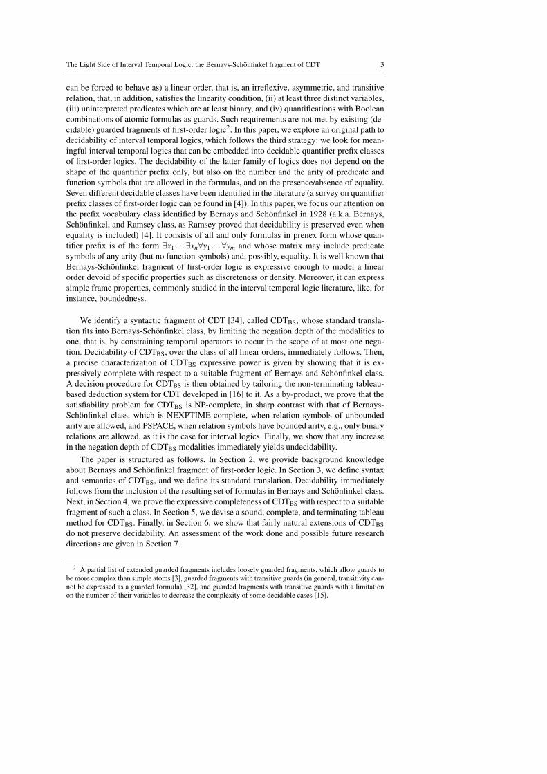
can be forced to behave as) a linear order, that is, an irreflexive, asymmetric, and transitiverelation, that, in addition, satisfies the linearity condition, (ii) at least three distinct variables,(iii) uninterpreted predicates which are at least binary, and (iv) quantifications with Booleancombinations of atomic formulas as guards. Such requirements are not met by existing (de-cidable) guarded fragments of first-order logic2. In this paper, we explore an original path todecidability of interval temporal logics, which follows the third strategy: we look for mean-ingful interval temporal logics that can be embedded into decidable quantifier prefix classesof first-order logics. The decidability of the latter family of logics does not depend on theshape of the quantifier prefix only, but also on the number and the arity of predicate andfunction symbols that are allowed in the formulas, and on the presence/absence of equality.Seven different decidable classes have been identified in the literature (a survey on quantifierprefix classes of first-order logic can be found in [4]). In this paper, we focus our attention onthe prefix vocabulary class identified by Bernays and Schonfinkel in 1928 (a.k.a. Bernays,Schonfinkel, and Ramsey class, as Ramsey proved that decidability is preserved even whenequality is included) [4]. It consists of all and only formulas in prenex form whose quan-tifier prefix is of the form ∃x1 . . .∃xn∀y1 . . .∀ym and whose matrix may include predicatesymbols of any arity (but no function symbols) and, possibly, equality. It is well known thatBernays-Schonfinkel fragment of first-order logic is expressive enough to model a linearorder devoid of specific properties such as discreteness or density. Moreover, it can expresssimple frame properties, commonly studied in the interval temporal logic literature, like, forinstance, boundedness.

We identify a syntactic fragment of CDT [34], called CDTBS, whose standard transla-tion fits into Bernays-Schonfinkel class, by limiting the negation depth of the modalities toone, that is, by constraining temporal operators to occur in the scope of at most one nega-tion. Decidability of CDTBS, over the class of all linear orders, immediately follows. Then,a precise characterization of CDTBS expressive power is given by showing that it is ex-pressively complete with respect to a suitable fragment of Bernays and Schonfinkel class.A decision procedure for CDTBS is then obtained by tailoring the non-terminating tableau-based deduction system for CDT developed in [16] to it. As a by-product, we prove that thesatisfiability problem for CDTBS is NP-complete, in sharp contrast with that of Bernays-Schonfinkel class, which is NEXPTIME-complete, when relation symbols of unboundedarity are allowed, and PSPACE, when relation symbols have bounded arity, e.g., only binaryrelations are allowed, as it is the case for interval logics. Finally, we show that any increasein the negation depth of CDTBS modalities immediately yields undecidability.

The paper is structured as follows. In Section 2, we provide background knowledgeabout Bernays and Schonfinkel fragment of first-order logic. In Section 3, we define syntaxand semantics of CDTBS, and we define its standard translation. Decidability immediatelyfollows from the inclusion of the resulting set of formulas in Bernays and Schonfinkel class.Next, in Section 4, we prove the expressive completeness of CDTBS with respect to a suitablefragment of such a class. In Section 5, we devise a sound, complete, and terminating tableaumethod for CDTBS. Finally, in Section 6, we show that fairly natural extensions of CDTBSdo not preserve decidability. An assessment of the work done and possible future researchdirections are given in Section 7.

2 A partial list of extended guarded fragments includes loosely guarded fragments, which allow guards tobe more complex than simple atoms [3], guarded fragments with transitive guards (in general, transitivity can-not be expressed as a guarded formula) [32], and guarded fragments with transitive guards with a limitationon the number of their variables to decrease the complexity of some decidable cases [15].


2 Bernays-Schonfinkel class

Bernays-Schonfinkel prefix vocabulary class, denoted here by FOBS, consists of all andonly those first-order formulas, making use of any relational symbol of any arity, includingequality, that can be put in prenex form by using a quantifier prefix of the form ∃x∀y,where x = x1 . . .xn and y = y1 . . .ym are (possibly empty) vectors of first-order variables. It iswell known that the satisfiability problem for FOBS is NEXPTIME-complete [4]. Moreover,FOBS is closed under conjunction and disjunction, since all its formulas can be thought of assentences (free variables can be existentially quantified), but it is not closed under negation.

To simplify the proofs of the results given in the paper, we introduce an alternativedefinition of FOBS via the following abstract grammar:

α ::= α∃ | α ∧α | α ∨α | ∃x.α | ¬α∃ for α∃ of the form ∃x.α∃ (1)

α∃ ::= A(x) | ¬A(x) | α∃∧α∃ | α∃∨α∃ | ∃x.α∃ (2)

A(x) ::= any relational symbol of arbitrary arity, including equality (3)

Grammar (1) generates a fragment of first-order logic consisting of all and only those for-mulas where existential quantifiers can occur in the scope of at most one negation. Whileany prenex formula of the form ∃x∀yβ can be generated by grammar (1), the converse is nottrue, since grammar (1) can generate also formulas which are not in prenex form. However,it is not difficult to show that any formula generated by grammar (1) can be transformed intoan equivalent prenex formula of the correct form, as shown by the following proposition.

Proposition 1 Any formula generated by grammar (1) can be transformed into a prenexformula of the form ∃x∀yβ , with β quantifier-free.

Proof Let α be a formula generated by grammar (1). We show that there exists an equivalentformula τ(α) of the required form by structural induction. We start with the set of formulasgenerated by the sub-grammar for α∃, and we show that each of them can be transformedinto a formula of the form ∃xβ , with β quantifier-free. The case in which α is a relationor the negation of a relation is trivial. Consider now the case of formulas α = α∃ ∧α ′∃.By inductive hypothesis, τ(α∃) = ∃zβ and τ(α ′∃) = ∃wβ ′, for some quantifier-free β andβ ′. Without loss of generality, we can assume z∩w = /0 (if this is not the case, we canapply a suitable variable substitution), and thus α is equivalent to ∃zw(β ∧β ′). The case ofdisjunction is similar, and thus omitted. Consider now the case of formulas α = ∃x.α∃. Byinductive hypothesis, τ(α∃) = ∃wβ , for some quantifier-free β , with x 6∈ w, and thus α isequivalent to ∃x∃wβ . Let us consider now an arbitrary formula generated by grammar (1).The only interesting case is the one for the negation of existential quantifiers. Let α =¬∃x.α∃. By inductive hypothesis, τ(∃x.α∃) = ∃x∃wβ , for some quantifier-free β , with x 6∈w. Hence, α is equivalent to the formula (in prenex form) ∀x∀w¬β . ut

Thanks to the above result, from now on we will assume that any FOBS-formula has beengenerated by grammar (1).

3 Decidability of the logic CDTBS over the class of all linear orders

Interval temporal logics are usually interpreted over a linearly ordered set D = 〈D,<〉. Inthis setting, an interval on D is an ordered pair [di,d j] with di ≤ d j (we refer to such a case as


di dk d j

C

Fig. 1 The ternary relation chop, splitting the interval [di,d j] into the subintervals [di,dk] and [dk,d j].

the non-strict semantics, in contrast with the strict one, that excludes degenerate intervals ofthe form [di,di]). The set of all intervals on D is denoted by I(D). The variety of all possiblerelations between any two intervals has been studied by Allen [1], who identified 12 distinctbinary relations plus the equality relation. Halpern and Shoham modal logic of intervals,abbreviated HS, can be viewed as the modal logic of Allen’s relations as it features onemodality for each such relation. As we already mentioned, HS turns out to be undecidableover any meaningful class of linear orders [20]. In [34], the ternary relation chop, depicted inFigure 1, has been taken into consideration. The corresponding binary modality C, togetherwith the two conjugated modalities D (done) and T (to do), and the modal constant π forpoint-intervals define the interval temporal logic CDT. It can be easily shown that CDTsubsumes HS (in fact, it is strictly more expressive than HS), and thus it is undecidablewhenever HS is. In [21], Hodkinson et al. systematically investigate the three fragmentsof CDT with only one binary modality each (C, D, or T ), showing that each of them isundecidable.

Formulas of CDT are built on a set of proposition letters A P = {p,q, . . .}, the Booleanconnectives ¬ and ∨, the three binary modalities C,D, and T , and the modal constant π , bythe following abstract grammar [34]:

ϕ ::= p | π | ¬ϕ | ϕ ∨ϕ | ϕ C ϕ | ϕ D ϕ | ϕ T ϕ.

The other Boolean connectives can be viewed as suitable short forms, as usual. Similarly,universal counterparts of the existential modalities C, D, and T can be defined by means ofnegation in the standard way; CDT has not any special notation for them.

The semantics of CDT-formulas can be given in terms of concrete models of the formM = 〈I(D),V 〉, where V : A P → 2I(D) is a valuation function, as follows:

– M, [di,d j] p if and only if [di,d j] ∈V (p),– M, [di,d j] π if and only if di = d j,– M, [di,d j] ¬ϕ if and only if M, [di,d j] 6 ϕ ,– M, [di,d j] ϕ ∨ψ if and only if M, [di,d j] ϕ or M, [di,d j] ψ ,– M, [di,d j] ϕ C ψ if and only if there exists di ≤ dk ≤ d j such that M, [di,dk] ϕ and

that M, [dk,d j] ψ ,– M, [di,d j] ϕ D ψ if and only if there exists dk ≤ di such that M, [dk,di] ϕ and that

M, [dk,d j] ψ ,– M, [di,d j] ϕ T ψ if and only if there exists dk ≥ d j such that M, [d j,dk] ϕ and that

M, [di,dk] ψ .

The standard translation is the usual way to express the semantics of a modal or tem-poral formula in first-order logic. Let ϕ be a CDT-formula and, for every p ∈ A P , let usdenote by the same symbol p the corresponding binary relation. The standard translationfunction ST (ϕ)[x,y] is defined as follows:

– ST (ϕ)[x,y] = x≤ y∧ST ′(ϕ)[x,y],

where x,y are two first-order variables and ST ′(ϕ)[x,y] is inductively defined as follows:

– ST ′(p)[x,y] = p(x,y),


– ST ′(π)[x,y] = (x = y),– ST ′(¬ϕ)[x,y] = ¬ST ′(ϕ)[x,y],– ST ′(ϕ ∨ψ)[x,y] = ST ′(ϕ)[x,y]∨ST ′(ψ)[x,y],– ST ′(ϕ C ψ)[x,y] = ∃z(x≤ z≤ y∧ST ′(ϕ)[x,z]∧ST ′(ψ)[z,y]),– ST ′(ϕ D ψ)[x,y] = ∃z(z≤ x∧ST ′(ϕ)[z,x]∧ST ′(ψ)[z,y]),– ST ′(ϕ T ψ)[x,y] = ∃z(y≤ z∧ST ′(ϕ)[y,z]∧ST ′(ψ)[x,z]).

As a general rule, the standard translation makes it possible to reduce the satisfiability prob-lem for a modal logic to a first-order satisfiability problem: a modal formula ϕ is satisfiableif and only if its standard translation, evaluated on a pair of points x,y, is (first-order) sat-isfiable. Now, we ask ourselves the following question: which CDT-formulas are such thattheir satisfiability problem can be reduced to a first-order satisfiability problem in Bernays-Schonfinkel class? To answer this question, we define an abstract grammar that generatesonly CDT-formulas suitably limited in the negation depth of modalities:

ϕ ::= ϕ∃ | ϕ ∧ϕ | ϕ ∨ϕ | ϕ C ϕ | ϕ D ϕ | ϕ T ϕ |¬(ϕ∃C ϕ∃) | ¬(ϕ∃D ϕ∃) | ¬(ϕ∃ T ϕ∃)

(4)

ϕ∃ ::= π | ¬π | p | ¬p | ϕ∃∧ϕ∃ | ϕ∃∨ϕ∃ | ϕ∃C ϕ∃ | ϕ∃D ϕ∃ | ϕ∃ T ϕ∃ (5)

The above grammar generates a fragment of CDT, that we call CDTBS, which consistsof all and only those formulas where the modalities C, D, and T can occur in the scope ofat most one negation. The next lemma shows that the above-defined standard translationmaps CDTBS-formulas into Bernays-Schonfinkel class. It is easy to check that the syntacticlimitations of CDTBS do not prevent it from expressing all HS modalities (it only constrainsthe way in which they can be composed). As an example, 〈B〉ϕ is captured by ϕ C ¬π .Similar encodings can be given for the other HS modalities [34].

Lemma 1 For every CDTBS-formula ϕ , its standard translation ST (ϕ)[x,y] is an FOBS-formula, with free variables x and y.

Proof The proof is by structural induction. We start with the set of formulas generated bythe sub-grammar for ϕ∃, and we show that the standard translation of each of these formulasbelongs to the sub-grammar for α∃ and it has x,y as its free variables.

As for the base case, let ϕ∃ = p, for some proposition letter p. By definition, ST (p)[x,y]= x ≤ y∧ p(x,y); the thesis immediately follows. The cases ¬p,π , and ¬π are similar,and thus omitted. As for the case of conjunction, let ϕ∃ = ϕ ′∃ ∧ϕ ′′∃ . By definition, ST (ϕ ′∃ ∧ϕ ′′∃ )[x,y] = x≤ y∧ST ′(ϕ ′∃)[x,y]∧ST ′(ϕ ′′∃ )[x,y]. By inductive hypothesis, both ST (ϕ ′∃)[x,y]and ST (ϕ ′′∃ )[x,y], and thus ST ′(ϕ ′∃)[x,y] and ST ′(ϕ ′′∃ )[x,y], belong to the sub-grammar forα∃ and have x,y as their free variables. It immediately follows that ST (ϕ ′∃∧ϕ ′′∃ )[x,y] has therequired form. The case of disjunction is similar, and thus omitted.

Now, let ϕ∃ = ϕ ′∃Cϕ ′′∃ . By definition, ST (ϕ ′∃C ϕ ′′∃ )[x,y] = x≤ y∧∃z(x≤ z≤ y∧ST ′(ϕ ′∃)[x,z]∧ST ′(ϕ ′′∃ )[z,y]). By inductive hypothesis, ST ′(ϕ ′∃)[x,z] is an α∃-formula with x,z as itsfree variables, and ST ′(ϕ ′′∃ )[z,y] is an α∃-formula with z,y as its free variables. Hence, theformula x≤ y∧∃z(x≤ z≤ y∧ST ′(ϕ ′∃)[x,z]∧ST ′(ϕ ′′∃ )[z,y]) is an α∃-formula with x,y as itsfree variables. The other two cases for D and T can be dealt with in a similar way.

Let us consider now an arbitrary formula generated by the grammar. The only in-teresting cases are those for the negation of modalities. Let ϕ = ¬(ϕ ′∃C ϕ ′′∃ ). By defini-tion, ST (¬(ϕ ′∃C ϕ ′′∃ ))[x,y] = x ≤ y∧¬ST ′(ϕ ′∃C ϕ ′′∃ )[x,y], and ST ′(ϕ ′∃C ϕ ′′∃ )[x,y] = ∃z(x ≤z ≤ y∧ ST ′(ϕ ′∃)[x,z]∧ ST ′(ϕ ′′∃ )[z,y]). We have already shown that both ST ′(ϕ ′∃)[x,z] andST ′(ϕ ′′∃ )[z,y] are α∃-formulas with x,z and z,y as their free variables, respectively. Hence,


∃z(x≤ z≤ y∧ST ′(ϕ ′∃)[x,z]∧ST ′(ϕ ′′∃ )[z,y]) is an α∃-formula with x,y as its free variables. Itimmediately follows that ¬ST ′(ϕ ′∃C ϕ ′′∃ )[x,y] is an α-formula with x,y as its free variables,and thus the thesis, as the conjunction of two α-formulas is an α-formula. The other twocases can be dealt with in a similar way. ut

In order to prove the main theorem, it suffices to observe that the linear order < is capturedby the following axioms [4], whose conjunction Φ belongs to FOBS:

1. ∀x¬(x < x);2. ∀x,y(x < y→¬y < x);3. ∀x,y,z(x < y∧ y < z→ x < z);4. ∀x,y(x = y∨ x < y∨ y < x).

Theorem 1 The satisfiability problem for CDTBS over the class of all linear orders is de-cidable.

Proof By Lemma 1, if ϕ is a CDTBS-formula, then ∃x,yST (ϕ)[x,y] (the existential closureof ST (ϕ)[x,y]) belongs to Bernays-Schonfinkel class. Satisfiability of ϕ can thus be reducedto satisfiability of the FOBS-formula Φ ∧∃x,yST (ϕ)[x,y]. Since the satisfiability problemfor FOBS is decidable, decidability of CDTBS immediately follows. ut

The satisfiability problem for FOBS has been shown to be NEXPTIME-complete. Theproof relies on the observation that an FOBS-formula is satisfiable if and only if it has amodel with a number of elements bounded by the number of existential quantifiers [4, Propo-sition 6.2.17]. This immediately leads to a nondeterministic exponential-time procedure forsatisfiability checking. However, when we restrict our attention to formulas where the arityof relational symbols is bounded (to two, in our case), the complexity of such a procedurebecomes PSPACE, since in this case a candidate model for the formula can be representedusing only a polynomial amount of memory. Hence, Theorem 1 gives us a PSPACE upper-bound to the complexity of CDTBS. In Section 5, we will show that this bound is not tight,by providing an NP decision procedure for the satisfiability of CDTBS.

4 Expressive completeness of CDTBS

In Section 3, we showed that CDTBS formulas can be translated into Bernays-Schonfin-kel class FOBS of first-order logic with equality, thanks to the fact that the linear order< can be expressed in this fragment. Inspired by the observation that the translation usesonly binary predicates, we now ask ourselves the following question: for every formula inBernays-Schonfinkel class of first-order logic, interpreted over the linear order < and limitedto binary predicates, is there an expressively equivalent CDTBS-formula? Similar expressiv-ity comparison issues have been already investigated for various point- and interval-basedlogics. A partial list includes basic results about the completeness of LTL with respect tothe first-order fragment of monadic second-order logic over Dedekind-complete linear or-ders and generalizations (Kamp’s Theorem and its extensions [12–14,22,23,26]), the com-pleteness of CDT with respect to the three-variable fragment of first-order logic over linearorders, where at most two variables are free [34], the completeness of AA with respect totwo-variable first-order logic over linear orders [8], and the completeness of its metric ex-tension, called MPNL, with respect to a fragment of two-variable first-order logic extendedwith a successor function over N [7].


We focus our attention on first-order logic interpreted over the linear order < and limitedto binary predicates, denoted by FO[<]. We will denote by FOn,m[<] the n-variable fragmentof FO[<], where at most m variables are free, and by FOω,m[<] the fragment of FO[<] witha denumerable set of variables, where at most m are free. Since interval logics are interpretedover intervals (represented as pairs of points), the standard translation of any interval logicformula is a formula with two free variables, and thus it belongs to FOω,2[<]. By analogywith the case of other interval logics, e.g., [8,34], to establish an expressive completenessresult for CDTBS, we will limit the number of variables of the corresponding first-order frag-ment. We denote by FOn,m

BS [<] (resp., FOω,mBS [<]) the n-variable fragment (resp., the fragment

with a denumerable set of variables) of the language defined by grammar (1), where at mostm variables occur free.

In the following, we compare interval and first-order logics with respect their abilityof expressing properties of a given interval in a model. We distinguish three cases: (i) thecomparison of two interval logics, (ii) the comparison of two fragments of first-order logic,and (iii) the comparison of an interval logic and a fragment of first-order logic.

Given two interval logics (resp., fragments of first-order logic) L and L’, we say that L’is at least as expressive as L, denoted by L � L′, if there is an effective translation τ fromL to L’, which is inductively defined on the structure of formulas, such that for every modelM, interval [di,d j] (resp., pair of points di,d j) in M, and formula ϕ of L, M, [di,d j] ϕ iffM, [di,d j] τ(ϕ) (resp., M |= ϕ(di,d j) iff M |= τ(ϕ)(di,d j)). Furthermore, we say that L’is as expressive as L, denoted by L′ ≡ L, if both L′ � L and L � L′, and we say that L’ isstrictly more expressive than L, denoted by L≺ L′, if L� L′ and L′ 6� L.

To compare the expressive power of an interval logic and a fragment of first-order logic,we must cope with a technical problem: interval models constrain interval logic formulasto be evaluated on ordered pairs [di,d j], with di ≤ d j, only, while relational models do notimpose such a constraint. To solve it, we map each binary relation p of the consideredfragment of first-order logic into two distinct proposition letters p≤ and p≥ of the intervallogic. From [8], we borrow the following definition.

Definition 1 Let M = 〈I(D),VM〉 be an interval model. The corresponding relational modelη(M) is the pair 〈D,Vη(M)〉, where, for every proposition letter p, Vη(M)(p) = {(a,b) ∈D×D : [a,b] ∈ VM(p)}. Conversely, let M = 〈D,VM〉 be a relational model. The correspondinginterval model ζ (M) is the pair 〈I(D),Vζ (M)〉, where, for every binary relation p and interval[di,d j], [di,d j]∈Vζ (M)(p≤) iff (di,d j)∈VM(p) and [di,d j]∈Vζ (M)(p≥) iff (d j,di)∈VM(p).

Given an interval logic LI and a fragment of first-order logic LFO, we say that LFO is at leastas expressive as LI , denoted by LI � LFO, if there exists an effective translation τ from LI toLFO such that for any interval model M, interval [di,d j], and LI-formula ϕ , M, [di,d j] ϕ iffη(M) |= τ(ϕ)(di,d j). Conversely, we say that LI is at least as expressive as LFO, denotedby LFO � LI , if there exists an effective translation τ ′ from LFO to LI such that, for anyrelational model M, pair of points (di,d j), and LFO-formula ϕ , M |= ϕ(di,d j) if and only ifζ (M), [di,d j] τ ′(ϕ), if di ≤ d j, or ζ (M), [d j,di] τ ′(ϕ), otherwise. LI ≡ LFO, LI ≺ LFO,and LFO ≺ LI are defined as usual.

In [33], Venema shows that the hierarchy of fragments FOn,2[<], for n≥ 2, is strict.

Theorem 2 For every n≥ 2, FOn,2[<] ≺ FOn+1,2[<] (over the class of all linear orders).

The expressive completeness of the interval logic of temporal neighborhood AA with respectto FO2,2[<] and of CDT with respect to FO3,2[<] have been proved by Bresolin et al. in [8]and by Venema in [34], respectively.


τ i, j(xi = x j) = π

τ i, j(x j = xi) = π

τ i, j(xi = xi) = >τ i, j(x j = x j) = >τ i, j(xi < x j) = ¬π

τ i, j(x j < xi) = ⊥τ i, j(xi < xi) = ⊥

τ i, j(x j < x j) = ⊥τ i, j(p(xi,x j)) = p≤

τ i, j(p(x j,xi)) = p≥

τ i, j(p(xi,xi)) = (π ∧ p≤)C>τ i, j(p(x j,x j)) = >C (π ∧ p≤)

τ i, j(¬α(xi,x j)) = ¬τ i, j(α(xi,x j))

τ i, j(α(xi,x j)∧β (xi,x j)) = τ i, j(α(xi,x j))∧ τ i, j(β (xi,x j))

τ i, j(α(xi,x j)∨β (xi,x j)) = τ i, j(α(xi,x j))∨ τ i, j(β (xi,x j))

τ i, j(∃xk(α(xi,xk)∧β (xk,x j))) = τk,i(α(xi,xk))D τk, j(β (xk,x j))∨τ i,k(α(xi,xk))C τk, j(β (xk,x j))∨τ j,k(β (xk,x j))T τ i,k(α(xi,xk))

Table 1 The mapping of FO3,2sp [<] into CDTBS: translation rules.

Theorem 3 AA≡ FO2,2[<].

Theorem 4 CDT ≡ FO3,2[<].

The proof of Theorem 2 consists of showing that, for any given n≥ 2, there exist two modelsM1 and M2 such that M1 and M2 satisfy the same set of FOn,2[<]-formulas, and there existsan FOn+1,2[<]-formula which is satisfied by M1 and not by M2. Equivalence of M1 and M2with respect to FOn,2[<]-formulas is established by a game-theoretic argument, while theFOn+1,2[<]-formula that differentiates the two models is the following one:

∃x1∃x2 . . .∃xn∃xn+1

( ∧xi 6=x j

¬p(xi,x j)). (6)

Since such a formula belongs to Bernays-Schonfinkel fragment of first-order logic, the verysame argument can be used to prove that FOn,2

BS [<] ≺ FOn+1,2BS [<], for any n≥ 2. Moreover,

by Theorem 4, it holds that FOn,2BS [<] ≺ FOn,2[<], for every n ≥ 3: on the one hand, it

trivially holds that FOn,2BS [<] � FOn,2[<]; on the other hand, decidability of FOω,2

BS [<] andundecidability of CDT imply that FOn,2[<] 6� FOn,2

BS [<]. Finally, we have that, for everyn≥ 3, FOn,2[<] and FOn+1,2

BS [<] are incomparable: on the one hand, FOn+1,2BS [<] 6� FOn,2[<],

as formula (6) belongs to FOn+1,2BS [<] and there is not an equivalent formula in FOn,2[<];

on the other hand, FOn+1,2BS [<] is decidable, while FOn,2[<] is not, and thus FOn,2[<] 6�

FOn+1,2BS [<]. Hence, the following theorem holds.

Theorem 5 For every n≥ 3, it holds that:

1. FOn−1,2BS [<] ≺ FOn,2

BS [<];2. FOn,2

BS [<] ≺ FOn,2[<];3. FOn,2[<] and FOn+1,2

BS [<] are incomparable

(over the class of all linear orders).

We conclude the section by showing that CDTBS is expressively complete with respectto FO3,2

BS [<]. One direction is straightforward: since the standard translation of CDTBS-formulas given in Section 3 makes use of 3 variables only, it holds that CDTBS � FO3,2

BS [<].We now show that the converse holds as well, that is, FO3,2

BS [<] � CDTBS. By analogyto the case of the mapping from FO3,2[<] to CDT defined by Venema [34], as a preliminarystep, we provide a suitable characterization of FO3,2

BS [<]-formulas.


Definition 2 Let {i, j,k} ⊆ {1,2,3}. The language FO3,2sp [<] is defined by the following

abstract grammar:

β (xi,x j) ::= β∃(xi,x j) | β (xi,x j)∧β (xi,x j) | β (xi,x j)∨β (xi,x j) |∃xk(β (xi,xk)∧β (xk,x j)) | ¬β∃(xi,x j) for β∃(xi,x j)

of the form ∃xk(β∃(xi,xk)∧β∃(xk,x j))

(7)

β∃(xi,x j) ::= A(xi,x j) | ¬A(xi,x j) | β∃(xi,x j)∧β∃(xi,x j) | β∃(xi,x j)∨β∃(xi,x j) |∃xk(β∃(xi,xk)∧β∃(xk,x j))

(8)

A(xi,x j) ::= xi = x j | x j = xi | xi = xi | x j = x j | xi < x j | x j < xi | xi < xi | x j < x j |p(xi,x j) | p(x j,xi) | p(xi,xi) | p(x j,x j)

(9)

Lemma 2 For every formula in FO3,2BS [<], there is an equivalent formula in FO3,2

sp [<].

Proof We prove the following stronger claim on the 3-variable fragment FO3,3BS [<], which

includes formulas where all three variables occur free:

for every formula α in FO3,3BS [<] there is equivalent formula τ(α), which is a

Boolean combination of FO3,2sp [<]-formulas, with the same free variables as α .

The proof is by structural induction.The base cases (α is an atomic formula or α is the negation of an atomic formula)

and the case of logical connectives (α is a conjunction or a disjunction of formulas) arestraightforward. In particular, as for the base case, it suffices to remind that we restricted ourattention to fragments of first-order logic with binary predicates only.

Let α be of the form ∃xkγ(xi,x j,xk). By the inductive hypothesis, γ(xi,x j,xk) is equiv-alent to a formula τ(γ(xi,x j,xk)), that we may assume, without loss of generality, to be adisjunction of conjunctions of formulas in FO3,2

sp [<]. By distributing the existential quan-tifier ∃xk over disjunctions, we obtain a formula of the form

∨mh=1∃xkγh(xi,x j,xk), where

each γh(xi,x j,xk) is a conjunction of formulas. Since only binary predicates are allowed,we can rewrite each γh(xi,x j,xk) as ξh(xi,x j)∧ξh(xi,xk)∧ξh(x j,xk). Since variable xk doesnot occur free in ξh(xi,x j), we can rewrite ∃xkγh(xi,x j,xk) as ξh(xi,x j)∧∃xk(ξh(xi,xk)∧ξh(x j,xk)). This latter formula is a conjunction of FO3,2

sp [<]-formulas with the same freevariables as α .

The case in which α is of the form ¬∃xkγ(xi,x j,xk) can be dealt with in a very similarway. ut

We are now ready to define the translation τ from FO3,2sp [<] to CDTBS. For the sake of

brevity, we write τ i, j for τ[xi,x j], with xi ≤ x j. Translation rules for atomic and complexformulas are given in Table 1.

Lemma 3 Let α(xi,x j) be an FO3,2sp [<]-formula. Then, for every pair of points (di,d j),

M |= α(di,d j) if and only if di ≤ d j and ζ (M), [di,d j] τ i, j(α(xi,x j)), or d j ≤ di andζ (M), [d j,di] τ j,i(α(xi,x j)).

Proof The proof is by induction on the structure of α(xi,x j). The cases of atomic formulasand Boolean connectives are straightforward.Once more, the only interesting case is the one of existential quantifiers. Let α(xi,x j) bethe formula ∃xk(β (xi,xk)∧ γ(xk,x j)) and di ≤ d j. By the semantic clauses for FO3,2

sp [<], it


FO2,2[<]

FO3,2[<]

FO4,2[<]

. . .

FOω,2[<]

FO3,2BS [<]

FO4,2BS [<]

. . .

FOω,2BS [<]

≡PNL ≡≡≡ CDTBS

≡CDT

Fig. 2 A classification of the considered interval logics and fragments of first-order logic with respect to theirexpressive power.

holds that M |= ∃xk(β (di,xk)∧ γ(xk,d j)) if and only if there exists a point dk such that M |=β (di,dk) and M |= γ(dk,d j). Since we are interpreting our formulas over a linear order, thereare three possible ways to place dk with respect to di and d j: either dk ≤ di, or di ≤ dk ≤ d j,or d j ≤ dk. By the inductive hypothesis, we have that M |= α(di,d j) if and only if:(

ζ (M), [dk,di] τk,i(β (xi,xk)) and ζ (M), [dk,d j] τ

k, j(γ(xk,x j)))

or(

ζ (M), [di,dk] τi,k(β (xi,xk)) and ζ (M), [dk,d j] τ

k, j(γ(xk,x j)))

or(

ζ (M), [d j,dk] τj,k(γ(xk,x j)) and ζ (M), [di,dk] τ

i,k(β (xi,xk))).

By the semantics of the C, D, and T operators, we can conclude that M |= α(di,d j) if andonly if ζ (M), [di,d j] τ i, j(α(xi,x j)), as required. ut

Theorem 6 CDTBS is as expressive as FO3,2BS [<].

Proof By Lemma 2 and Lemma 3, FO3,2BS [<] � FO3,2

sp [<] � CDTBS. Moreover, by Lemma1, CDTBS � FO3,2

BS [<]. Hence, CDTBS ≡ FO3,2BS [<]. ut

Figure 2 gives a graphical account of the relationships among the considered logics(interval logics and fragments of first-order logic) in terms of their expressive power (thecontributions of the present work are in boldface).

5 A tableau method for CDTBS

In [16], Goranko et al. propose a tableau method for CDT interpreted over partial orders withthe linear interval property, that is, partial orders in which every interval is linear (BCDT+

for short). The method provides a semi-decision procedure for BCDT+ (it is not guaranteedto terminate). This does not come as a surprise as BCDT+ is undecidable. In this section,we show how to turn the method into an NP decision procedure CDTBS. In particular, weshow how to exploit BCDT+ syntactic restrictions to guarantee termination.

Let us start with some basic terminology. A finite tree is a finite directed acyclic graphin which every node, apart from one (the root), has exactly one incoming edge. A successorof a node n is a node n′ such that there is an edge from n to n′. A leaf is a node with no


successors. A path is a sequence of nodes n0, . . . ,nk such that, for all i = 0 . . .k−1, ni+1 isa successor of ni; a branch is a path from the root to a leaf. The height of a node n is themaximum length (number of edges) of a path from n to a leaf, while its depth is the lengthof the (unique) path from the root to it. If two nodes n and n′ belong to the same branchand the height of n is less than (resp., less than or equal to) the height of n′, we write n≺ n′

(resp., n� n′).

Definition 3 Let D be a finite linear order. A labeled formula over D is a pair (ψ, [di,d j]),where ψ ∈ CDTBS and [di,d j] ∈ I(D).

Definition 4 Let T be a (finite) tree and let n be a node of T . The decoration ν(n) of n isa tuple 〈ψ, [di,d j],D, p,u〉, where D is a finite linear order, (ψ, [di,d j]) is a labeled formulaover D, p ∈ {0,1}, and u is a local flag function which associates the values 0 or 1 withevery branch B containing n.

Definition 5 A decorated tree is a finite tree T enriched with a decoration ν(n) for eachnode n of T , apart from the root.

The tableau construction described below generates a decorated tree T . Given a branch Band a node n belonging to it, with decoration ν(n), u(B)= 1 means that n can be expanded onB. Given a branch B, B · (n1 · . . . ·nh) is the result of the expansion of B with the sequence ofnodes n1 · . . . ·nh (for h= 1, we simply write B ·n), while B ·(n1,1 · . . . ·n1,h)| . . . |(nk,1 · . . . ·nk,h)is the result of the expansion of B with k sequences of h nodes (for h = 1, we simply writeB · n1| . . . |nk). The auxiliary flag p has been added to simplify termination and complexityproofs. It records the nature of formula ψ: if ψ is a ϕ∃-formula, then p= 0; otherwise, p= 1.Finally, if n is the leaf of a branch B, we denote by DB the finite linear order in ν(n).

Since in CDTBS negation can occur only in front of proposition letters or modalities, weneed to introduce the notion of dual formula of a formula ϕ , denoted by ϕ . It is inductivelydefined as follows:

– p = ¬p and ¬p = p, for every p ∈A P ∪{π};– ϕ ∨ψ = ϕ ∧ψ;– ϕ ∧ψ = ϕ ∨ψ;– ϕ R ψ = ¬(ϕ R ψ), for R ∈ {C,D,T};– ¬(ϕ R ψ) = ϕ R ψ , for R ∈ {C,D,T}.

Notice that the dual of a generic CDTBS-formula does not necessarily belong to CDTBS.This is the case, for instance, with the formula pC¬(qC r). However, the following lemmaguarantees that dual formulas of ϕ∃-formulas are CDTBS-formulas. Such a lemma will playa crucial role in the proof of correctness of the tableau method.

Lemma 4 Let ϕ be a ϕ∃-formula. Then, ϕ is a CDTBS-formula.

Proof The cases of proposition letters and Boolean connectives can be proved by a straight-forward structural induction. To prove that the thesis holds also for modalities, let us assumeϕ = ψ C τ to be a ϕ∃-formula. By definition, the dual formula ϕ is ¬(ψ C τ). Since ψ,τ areϕ∃-formulas, we can conclude that ϕ is a CDTBS-formula. The other cases can be dealt within a similar way. ut

The construction of a tableau for a CDTBS-formula ϕ to be checked for satisfiability startsfrom a three-node tree (initial tableau) consisting of a root and two leaves with decorations〈ϕ, [d0, d0],{d0},1,1〉 and 〈ϕ, [d0,d1],{d0 < d1},1,1〉, respectively. The procedure exploits


a set of expansion rules, adapted from those given in [16], to add new nodes to the tree.In particular, the original rules for modalities have been revised to restrict the search forpossible models to linear orders only.

Definition 6 Given a tree T , a branch B in T , and a node n∈ B with decoration 〈ψ, [di,d j],D, pn,un〉 such that un(B) = 1, the branch-expansion rule for B and n is defined as follows(in all considered cases, un′(B′) = 1 for all new nodes n′ and branches B′).

R1 If ψ = ξ0∧ξ1, then expand B to B ·n0 ·n1, where n0 is decorated with 〈ξ0, [di,d j],DB, pn,un0〉 and n1 is decorated with 〈ξ1, [di,d j],DB, pn,un1〉.

R2 If ψ = ξ0∨ξ1, then expand B to B ·n0 | n1, where n0 is decorated with 〈ξ0, [di,d j],DB, pn,un0〉 and n1 is decorated with 〈ξ1, [di,d j],DB, pn,un1〉.

R3 If ψ = ¬(ξ0 C ξ1) and d is a point in DB, with di ≤ d ≤ d j, which has not beenused yet to expand n in B, then expand B to B · n0|n1, where n0 is decorated with〈ξ0, [di,d],DB,0,un0〉 and n1 is decorated with 〈ξ1, [d,d j],DB,0,un1〉.

R4 If ψ =¬(ξ0 Dξ1), and d is a point in DB, with d ≤ di, which has not been used yet to ex-pand n in B, then expand B to B ·n0|n1, where n0 is decorated with 〈ξ0, [d,di],DB,0,un0〉and n1 is decorated with 〈ξ1, [d,d j],DB,0,un1〉.

R5 If ψ =¬(ξ0 T ξ1), and d is a point in DB, with d j ≤ d, which has not been used yet to ex-pand n in B, then expand B to B ·n0|n1, where n0 is decorated with 〈ξ0, [d j,d],DB,0,un0〉and n1 is decorated with 〈ξ1, [di,d],DB,0,un1〉.

R6 If ψ = ξ0 C ξ1, then expand B to B · (ni ·mi)| . . . |(n j ·m j)|(n′i ·m′i)| . . . |(n′j−1 ·m′j−1),where:

(a) for all i ≤ k ≤ j, nk is decorated with 〈ξ0, [di,dk],DB, pn,unk〉 and mk is decoratedwith 〈ξ1, [dk,d j],DB, pn,umk〉;

(b) for all i≤ k ≤ j−1, Dk is the linear ordering obtained from DB by inserting a newpoint d between dk and dk+1, n′k is decorated with 〈ξ0, [di,d],Dk, pn,un′k

〉 and m′k isdecorated with 〈ξ1, [d,d j],Dk, pn,um′k

〉.

R7 If ψ = ξ0 D ξ1 and d0 is the least point of DB, then expand B to B · (n0 ·m0)| . . . |(ni ·mi)|(n′0 ·m′0)| . . . |(n′i ·m′i), where:

(a) for all 0 ≤ k ≤ i, nk is decorated with 〈ξ0, [dk,di],DB, pn,unk〉 and mk is decoratedwith 〈ξ1, [dk,d j],DB, pn,umk〉;

(b) for all 0≤ k≤ i, Dk is the linear ordering obtained from DB by inserting a new pointd between dk−1 and dk (for k = 0, d is placed immediately before d0), n′k is decoratedwith 〈ξ0, [d,di],Dk, pn,un′k

〉 and m′k is decorated with 〈ξ1, [d,d j],Dk, pn,um′k〉.

R8 If ψ = ξ0 T ξ1 and dN is the greatest point of DB, then expand B to B · (n j ·m j)| . . . |(nN ·mN)|(n′j ·m′j)| . . . |(n′N ·m′N), where:

(a) for all j ≤ k ≤ N, nk is decorated with 〈ξ0, [d j,dk],DB, pn,unk〉 and mk is decoratedwith 〈ξ1, [di,dk],DB, pn,umk〉;

(b) for all j≤ k≤N, Dk is the linear ordering obtained from DB by inserting a new pointd between dk and dk+1 (for k = N, d is placed immediately after dN), n′k is decoratedwith 〈ξ0, [d j,d],Dk, pn,un′k

〉 and m′k is decorated with 〈ξ1, [di,d],Dk, pn,um′k〉.

Finally, for each branch B′ extending B, let um(B′) = um(B), for each node m 6= n in B,and let un(B′) = 0, unless ψ = ¬(ξ0Cξ1), ψ = ¬(ξ0Dξ1), or ψ = ¬(ξ0T ξ1) (in such casesun(B′) = 1).


We briefly explain the behavior of the branch-expansion rule in cases R6 (ξ0 C ξ1) and R3(¬(ξ0Cξ1)). The corresponding cases for modalities D and T are similar. R6 deals with twopossible scenarios: either there exists dk ∈ DB such that ξ0 holds over [di,dk] and ξ1 holdsover [dk,d j], or such a point must be added to DB. The successors (ni ·mi)| . . . |(n j ·m j)created by the rule cover the former case, while the successors (n′i ·m′i)| . . . |(n′j−1 ·m′j−1)cover the latter case. As for R3, the formula ¬(ξ0 C ξ1) states that, for all di ≤ d ≤ d j,either ξ0 holds over [di,d] or ξ1 holds over [d,d j]. R3 imposes such a condition for a singlepoint d ∈ DB and keeps the flag equal to 1. In such a way, all points in DB are eventuallyconsidered, including those points that will be added in subsequent steps of the tableauconstruction.

Definition 7 A branch B is closed if one of the following conditions holds:

1. there are two nodes n,n′ in B such that ν(n) = 〈ψ, [di,d j],D, p,u〉 and ν(n′) =〈ψ, [di,d j],D′, p′,u′〉 for some formula ψ and di,d j ∈ D;

2. there is a node n such that ν(n) = 〈π, [di,d j],D, p,u〉 and di 6= d j;3. there is a node n such that ν(n) = 〈¬π, [di,d j],D, p,u〉 and di = d j;

If none of the above conditions hold, the branch is open.

Definition 8 The branch-expansion strategy for a branch B in a decorated tree T is definedas follows:

1. apply the branch-expansion rule to a branch B only if it is open;2. if B is open, apply the branch-expansion rule to the closest to the root node n such

that un(B) = 1 and the application of the rule generates at least one node with a newdecoration (if any).

Definition 9 A tableau T is any decorated tree obtained from the initial tableau by theapplication of the branch-expansion strategy.

We say that a tableau T is closed if and only if all its branches are closed, otherwise it isopen.

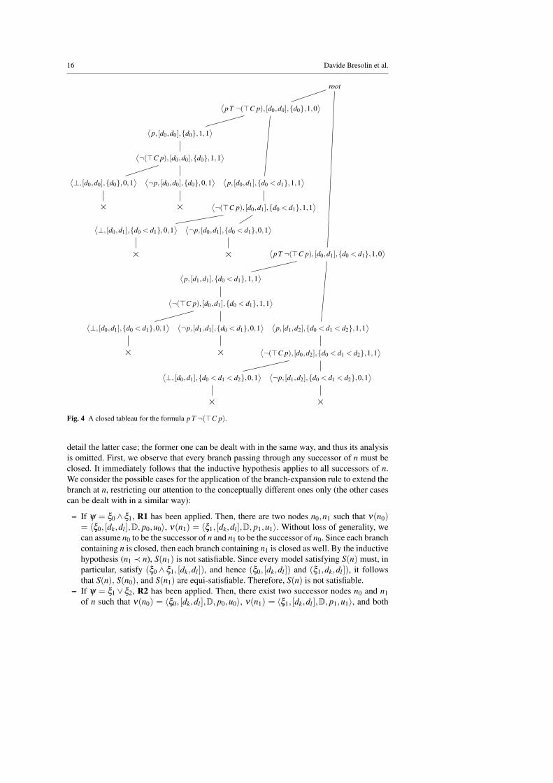
We conclude the section by giving a couple of examples of the application of the pro-posed method. As a first example, we consider the satisfiable formula ϕ = (¬π D¬π)C¬π .A portion of a tableau for ϕ is given in Figure 3, where thick edges highlights an openbranch representing a four-point model for the formula. As a second example, let ψ be theunsatisfiable formula p T ¬(>C p). A closed tableau for ψ is given in Figure 4. It is worthpointing out that there is an abuse of notation in the last component of the node decorations:while it is formally defined as a function from a set of branches to {0,1}, in the pictures itis represented as a constant (either 0 or 1). The reason is that in the proposed examples thefunction is constant for each node, that is, for each n we have that the value of the functionun(B) is the same for every branch B containing n.

In the following, we will show that to establish the satisfiability of a CDTBS-formulaϕ it is sufficient to start with the initial tableau for ϕ , and keep expanding it for as longas it is possible: if the resulting tableau is open, then ϕ is satisfiable, otherwise it is not.Moreover, we will prove that this expansion procedure terminates and it can be executed bya nondeterministic machine that uses only a polynomial amount of time.


root

⟨(¬π D¬π)C¬π, [d0,d0],{d0},1,0

⟩⟨¬π D¬π, [d0,d0],{d0},1,1

⟩⟨¬π, [d0,d0],{d0},1,1

⟩×

⟨(¬π D¬π)C¬π, [d0,d1],{d0 < d1},1,0

⟩

⟨¬π D¬π, [d0,d0],{d0 < d1},1,1

⟩⟨¬π, [d0,d1],{d0 < d1},1,1

⟩· · ·

⟨¬π D¬π, [d0,d1],{d0 < d1},1,1

⟩⟨¬π, [d1,d1],{d0 < d1},1,1

⟩×

⟨¬π D¬π, [d0,d2],{d0 < d2 < d1},1,0

⟩⟨¬π, [d2,d1],{d0 < d2 < d1},1,1

⟩

⟨¬π, [d0,d2],{d0 < d2 < d1},1,1

⟩⟨¬π, [d0,d0],{d0 < d2 < d1},1,1

⟩×

⟨¬π, [d3,d0],{d3 < d0 < d2 < d1},1,1

⟩⟨¬π, [d3,d2],{d3 < d0 < d2 < d1},1,1

⟩

Fig. 3 A portion of an open tableau for the formula (¬π D¬π)C¬π .

5.1 Soundness

In this subsection, we prove that the proposed tableau method is sound, that is, given aformula ϕ and a tableau T for it, if T is closed, then ϕ is not satisfiable. In the nextsubsection, we will show that the method is also complete.

Lemma 5 (Soundness) Let ϕ be a CDTBS-formula and T be a tableau for it. If T isclosed, then ϕ is not satisfiable.

Proof Let n be a node in the tableau T , and let Dn = {d0 < .. . < ds} be the linear orderingfrom ν(n). We will prove the following claim by induction on the height h of the node:

if every branch including n is closed, then the set S(n) of all labeled formulas in thedecorations of the nodes between n and the root is neither satisfiable in I(Dn) norin any extension of it.

If h = 0, then n is a leaf and the unique branch B containing n is closed. Then, eitherS(n) contains both the labeled formulas (ψ, [dk,dl ]) and (¬ψ, [dk,dl ]), for some CDTBS-formula ψ and dk,dl ∈ Dn, or the labeled formula (π, [dk,dl ]), for some dk 6= dl , or thelabeled formula (¬π, [dk,dl ]), for some dk = dl . Take any model M = 〈I(D′),V 〉, whereD′ extends Dn. It holds that M, [dk,dl ] ψ if and only if M, [dk,dl ] 6 ¬ψ , and, therefore,(ψ, [dk,dl ]) and (¬ψ, [dk,dl ]) cannot be jointly satisfied. Similarly, M, [dk,dl ] π (resp.,M, [dk,dl ] ¬π) if and only if dk = dl (resp., dk 6= dl), and therefore (π, [dk,dl ]) (resp.,(¬π, [dk,dl ])) cannot be satisfied when dk 6= dl (resp., dk = dl).

Now, suppose that h > 0. Then, either n has been generated as one of the successors,but not the last one, when applying cases R1, R6, R7, or R8 of the branch-expansion rule,or the branch-expansion rule has been applied to some labeled formula (ψ, [dk,dl ]) ∈ S(n)\{τ}, where τ is the labeled formula in the decoration ν(n), to extend the branch at n. We


root

⟨p T ¬(>C p), [d0,d0],{d0},1,0

⟩⟨

p, [d0,d0],{d0},1,1⟩

⟨¬(>C p), [d0,d0],{d0},1,1

⟩⟨¬p, [d0,d0],{d0},0,1

⟩×

⟨⊥, [d0,d0],{d0},0,1

⟩×

⟨p, [d0,d1],{d0 < d1},1,1

⟩⟨¬(>C p), [d0,d1],{d0 < d1},1,1

⟩⟨⊥, [d0,d1],{d0 < d1},0,1

⟩×

⟨¬p, [d0,d1],{d0 < d1},0,1

⟩× ⟨

p T ¬(>C p), [d0,d1],{d0 < d1},1,0⟩

⟨p, [d1,d1],{d0 < d1},1,1

⟩⟨¬(>C p), [d0,d1],{d0 < d1},1,1

⟩⟨¬p, [d1,d1],{d0 < d1},0,1

⟩×

⟨⊥, [d0,d1],{d0 < d1},0,1

⟩×

⟨p, [d1,d2],{d0 < d1 < d2},1,1

⟩⟨¬(>C p), [d0,d2],{d0 < d1 < d2},1,1

⟩⟨¬p, [d1,d2],{d0 < d1 < d2},0,1

⟩×

⟨⊥, [d0,d1],{d0 < d1 < d2},0,1

⟩×

Fig. 4 A closed tableau for the formula p T ¬(>C p).

detail the latter case; the former one can be dealt with in the same way, and thus its analysisis omitted. First, we observe that every branch passing through any successor of n must beclosed. It immediately follows that the inductive hypothesis applies to all successors of n.We consider the possible cases for the application of the branch-expansion rule to extend thebranch at n, restricting our attention to the conceptually different ones only (the other casescan be dealt with in a similar way):

– If ψ = ξ0 ∧ ξ1, R1 has been applied. Then, there are two nodes n0,n1 such that ν(n0)= 〈ξ0, [dk,dl ],D, p0,u0〉, ν(n1) = 〈ξ1, [dk,dl ],D, p1,u1〉. Without loss of generality, wecan assume n0 to be the successor of n and n1 to be the successor of n0. Since each branchcontaining n is closed, then each branch containing n1 is closed as well. By the inductivehypothesis (n1 ≺ n), S(n1) is not satisfiable. Since every model satisfying S(n) must, inparticular, satisfy (ξ0 ∧ ξ1, [dk,dl ]), and hence (ξ0, [dk,dl ]) and (ξ1,dk,dl ]), it followsthat S(n), S(n0), and S(n1) are equi-satisfiable. Therefore, S(n) is not satisfiable.

– If ψ = ξ1 ∨ ξ2, R2 has been applied. Then, there exist two successor nodes n0 and n1of n such that ν(n0) = 〈ξ0, [dk,dl ],D, p0,u0〉, ν(n1) = 〈ξ1, [dk,dl ],D, p1,u1〉, and both


n0≺ n and n1≺ n. Since each branch containing n is closed, then each branch containingn0 or n1 is closed as well. By the inductive hypothesis, S(n0) and S(n1) are not satisfi-able. Since every model satisfying S(n) must also satisfy (ξ0, [dk,dl ]) or (ξ1, [dk,dl ]), itfollows that S(n) is not satisfiable.

– If ψ = ¬(ξ0 C ξ1), R3 has been applied. For the sake of contradiction, let us assumeS(n) to be satisfiable. Then, since (¬(ξ0 Cξ1), [dk,dl ]) ∈ S(n), there is a model M =〈I(D′),V 〉 such that D′ extends Dn and M, [dk,dl ] ¬(ξ0Cξ1). Hence, for each dt suchthat dk ≤ dt ≤ dl , M, [dk,dt ] 6 ξ0 or M, [dt ,dl ] 6 ξ1. By construction, the two immediatesuccessors of n are two nodes n0 and n1 and there exists a point dt , with dk≤ dt ≤ dl , suchthat (ξ 0, [dk,dt ]) is in ν(n0) and (ξ 1, [dt ,dl ]) is in ν(n1). By the inductive hypothesis(both n0 ≺ n and n1 ≺ n), S(n0) and S(n1) are not satisfiable. But, from the hypothesisof our reductio-ad-absurdum argument, there is a model M = 〈I(D′),V 〉, where D′ is anextension of Dn, such that M, [dk,dt ] ¬ξ0 or M, [dt ,dl ] ¬ξ1. Thus, either S(n0) orS(n1) is satisfiable (by model M), leading to a contradiction.

– If ψ = ξ0 C ξ1, R6 has been applied. For the sake of contradiction, let us assume S(n)to be satisfiable. Then, there is a model M = 〈I(D′),V 〉 such that D′ extends Dn andM, [dk,dl ] ξ0 C ξ1. Hence, M, [dk,d] ξ0 and M, [d,dl ] ξ1 for some dk ≤ d ≤ dl .Two cases are possible:

1. If d ∈ Dn, then d = dt for some dk ≤ dt ≤ dl . By R6, n has a successor, say it nt ,which, in turn, has a successor, say it n′t , with ν(nt) = 〈ξ0, [dk,dt ],Dn, pt ,ut〉 andν(n′t) = 〈ξ1, [dt ,dl ],Dn, p′t ,u

′t〉. By the inductive hypothesis (nt ≺ n and n′t ≺ nt ),

S(n′t) = S(n)∪{(ξ0, [dk,dt ]),(ξ1, [dt ,dl ])} is not satisfiable. But, from the hypothesisof our reductio-ad-absurdum argument, there is a model M = 〈I(D′),V 〉, where D′is an extension of Dn, such that M, [dk,dt ] ξ0 and M, [dt ,dl ] ξ1. Thus, S(n′t) issatisfiable (by model M), leading to a contradiction.

2. If d /∈ Dn, then there exists t such that k ≤ t ≤ l−1 and dt < d < dt+1. By R6,n has a successor, say it nt , which, in turn, has a successor, say it n′t , with ν(nt)= 〈ξ0, [dk,d],Dn ∪{d}, pt ,ut〉, ν(n′t) = 〈ξ1, [d,dl ],Dn ∪{d}, p′t ,u

′t〉. By the induc-

tive hypothesis (nt ≺ n and n′t ≺ nt ), S(n′t) = S(n) ∪{(ξ0, [dk,d]),(ξ1, [d,dl ])} is notsatisfiable, which, as in the previous case, leads to a contradiction. ut

5.2 Completeness

In this subsection, we prove that the proposed tableau method is complete, that is, wheneverϕ ∈ CDTBS is valid, every tableau T for ¬ϕ must be closed. To this end, we need topreliminary prove some partial results.

Definition 10 Let ϕ be a CDTBS-formula and T0 be the initial tableau for it. The limittableau T for φ is the decorated tree generated as follows. For all i ≥ 0, let Ti+1 be thetableau generated by the simultaneous application of the branch-expansion strategy to eachbranch in Ti. If we ignore all flags from the decorations of the nodes in every Ti, we obtaina chain of decorated trees ordered by inclusion: T1 ⊆T2 ⊆ . . .⊆Tk ⊆ . . .. The limit tableau

T is equal toω⋃

i=0Ti.

Notice that the above definition does not prelude the limit tableau from being infinite. Lateron, we will prove that it cannot be the case, that is, the limit tableau is always finite. Never-theless, finiteness (of the limit tableau) is not necessary to prove that the tableau method iscomplete.


The definitions of open and closed branch and tableau directly apply to the limit tableauas well. In addition, we introduce the notion of saturated branch and tableau.

Definition 11 A branch in a (limit) tableau is saturated if there are no nodes on that branchto which the branch-expansion rule is applicable on the branch. A (limit) tableau is saturatedif every open branch in it is saturated.

We now show that the set of all labeled formulas on an open branch in a limit tableauhas the saturation properties of a Hintikka set in first-order logic.

Lemma 6 Every limit tableau is saturated.

Proof Let B be a branch B in the limit tableau T and n be a node in B. We prove thatafter every step of the expansion of that branch at which the branch-expansion rule becomesapplicable to n (because n has just been introduced or a new point has been added) and theapplication of the rule generates at least a new node, then that rule is subsequently appliedon B to that node. The proof is by induction on depth(n) (the depth of node n).

Let us assume that depth(n) = l and the branch-expansion rule has become applica-ble to n. By the inductive hypothesis, the thesis holds for all nodes with depth(n) < l.If there are no nodes between the root (including the root) and n (excluding n) to whichthe branch-expansion rule is applicable at that moment, the next application of the branch-expansion rule on B is necessarily to n. Otherwise, let n∗ be the closest-to-n node betweenthe root and n to which the branch-expansion rule is applicable, or will become applica-ble, on B at least once thereafter. (Such a node exists because there are only finitely manynodes between n and the root.) Since depth(n∗) < depth(n), by the inductive hypothesis,the branch-expansion rule has been subsequently applied to n∗. Then, the next applicationof the branch-expansion rule on B must have been to n and that completes the induction.

Suppose now that there exists a branch B in a limit tableau which is not saturated. Letn be the closest-to-the-root node on B to which the branch-expansion rule is applicable. Ifthe case applicable to n is different from R3, R4, and R5, then the branch-expansion rulehas become applicable to n at the step when n is introduced, and by the claim above, ithas been subsequently applied. Hence, the node has become unavailable thereafter, whichcontradicts the assumption. Let us consider now the case of R3, that is, the formula in ν(n) is¬(ξ0 C ξ1) (cases R4 and R5 are similar, and thus they are omitted). An application of R3 onB would create two immediate successors with labeled formulas (ξ 0, [di,d]) and (ξ 1, [d,d j]),at least one of them new on B. For R3 to be applicable, points di,d j, and d must have beenalready introduced at some step of the construction of B. Hence, at the moment when thethree of them, and n, have appeared on the branch, the branch-expansion rule has becomeapplicable to n. By the above claim, the rule has been subsequently applied on B and suchan application must have introduced the labeled formulas (ξ0, [di,d]) and (ξ1, [d,d j]) on B,which again contradicts the assumption. ut

Corollary 1 Let ϕ be a CDTBS-formula and T be the limit tableau for ϕ . For every openbranch B in T , the following closure properties hold:

– If there is a node n ∈ B such that ν(n) = (ξ0 ∧ ξ1, [di,d j],D, pn,un), then there are anode n0 ∈ B such that ν(n0) = (ξ0, [di,d j],D, pn0 ,un0) and a node n1 ∈ B such thatν(n1) = (ξ1, [di,d j],D, pn1 ,un1).

– If there is a node n ∈ B such that ν(n) = (ξ0 ∨ ξ1, [di,d j],D, pn,un), then there are anode n0 ∈ B such that ν(n0) = (ξ0, [di,d j],D, pn0 ,un0) or a node n1 ∈ B such that ν(n1)= (ξ1, [di,d j],D, pn1 ,un1).


– If there is a node n ∈ B such that ν(n) = (ξ0 C ξ1, [di,d j],D, pn,un), then there are twonodes n0,n1 ∈ B such that ν(n0) = (ξ0, [di,d],D′, pn0 ,un0) and ν(n1) = (ξ1, [d,d j],D′,pn0 ,un0), for some d ∈ DB, with di ≤ d ≤ d j, .

– If there is a node n ∈ B such that ν(n) = (ξ0 D ξ1, [di,d j],D, pn,un), then there are twonodes n0,n1 ∈ B such that ν(n0) = (ξ0, [d,di],D′, pn0 ,un0) and ν(n1) = (ξ1, [d,d j],D′,pn0 ,un0), for some d ∈ DB, with d ≤ di.

– If there is a node n ∈ B such that ν(n) = (ξ0 T ξ1, [di,d j],D, pn,un), then there are twonodes n0,n1 ∈ B such that ν(n0) = (ξ0, [di,d],D′, pn0 ,un0) and ν(n1) = (ξ1, [d j,d],D′,pn0 ,un0), for some d ∈ DB, with d ≥ d j, .

– If there is a node n ∈ B such that ν(n) = (¬(ξ0 C ξ1), [di,d j],D, pn,un), then, for eachd ∈ DB, with di ≤ d ≤ d j, there is a node n′ ∈ B such that ν(n′) = (ξ 0, [di,d],D′, pn′ ,

un′) or a node n′ ∈ B such that ν(n′) = (ξ 1, [d,d j],D′, pn′ ,un′).– If there is a node n ∈ B such that ν(n) = (¬(ξ0 D ξ1), [di,d j],D, pn,un), then for each

d ∈ DB, with d ≤ di, there is a node n′ ∈ B such that ν(n′) = (ξ 0, [d,di],D′, pn′ , un′) ora node n′ ∈ B such that ν(n′) = (ξ 1, [d,d j],D′, pn′ ,un′).

– If there is a node n ∈ B such that ν(n) = (¬(ξ0 T ξ1), [di,d j],D, pn,un), then, for eachd ∈ DB, with d ≥ d j, there is a node n′ ∈ B such that ν(n′) = (ξ 0, [di,d],D′, pn′ , un′) ora node n′ ∈ B such that ν(n′) = (ξ 1, [d j,d],D′, pn′ ,un′).

The proof of Corollary 1 is straightforward, and thus it is omitted.

Lemma 7 (Completeness) If the limit tableau for some formula ϕ ∈ CDTBS is closed, thensome finite tableau for ϕ is closed.

Proof Let us assume the limit tableau for ϕ to be closed. Then, every branch closes at somefinite step of the construction, and then it is not further expanded (it remains finite). Sincethe branch-expansion rule always produces finitely many successors, every finite tableauis finitely branching, and hence so is the limit tableau. Then, by Konig’s lemma, the limittableau, being a finitely branching tree with no infinite branches, must be finite. This allowsus to conclude that its construction stabilizes at some finite stage. At that stage, a closedtableau for ϕ is constructed. ut

5.3 Termination and Complexity

In this last subsection, we prove that the proposed tableau method is terminating, and wedetermine its computational complexity. The proof rests on a pair of basic lemmas.

As a preliminary step, we define a counting function Count on B as follows:

Count(B) = ∑n∈B|ψn| · pn ·un(B),

where ψn and pn are the formula and the p-flag in the decoration of n, respectively. Thefollowing lemma proves that Count is non-increasing with respect to branch expansions.

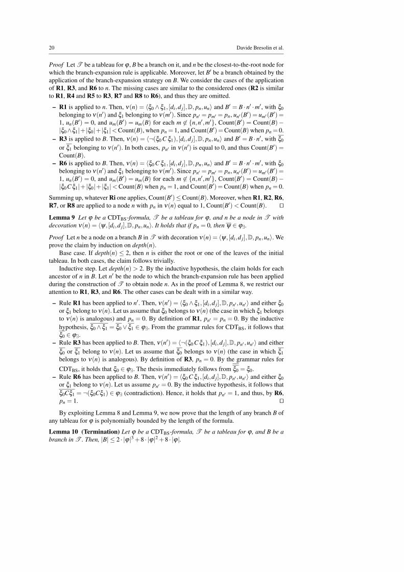
Lemma 8 Let ϕ be a CDTBS-formula, B be a branch in a tableau for ϕ , and B′ be anexpansion of B generated by the application of the branch-expansion strategy of Definition8. Then, Count(B′)≤ Count(B). Moreover, if B′ is obtained from B by the application of R1,R2, R6, R7, or R8 to a node n with pn in ν(n) equal to 1, then Count(B′)< Count(B).


Proof Let T be a tableau for ϕ , B be a branch on it, and n be the closest-to-the-root node forwhich the branch-expansion rule is applicable. Moreover, let B′ be a branch obtained by theapplication of the branch-expansion strategy on B. We consider the cases of the applicationof R1, R3, and R6 to n. The missing cases are similar to the considered ones (R2 is similarto R1, R4 and R5 to R3, R7 and R8 to R6), and thus they are omitted.

– R1 is applied to n. Then, ν(n) = 〈ξ0 ∧ ξ1, [di,d j],D, pn,un〉 and B′ = B ·n′ ·m′, with ξ0belonging to ν(n′) and ξ1 belonging to ν(m′). Since pn′ = pm′ = pn, un′(B′) = um′(B′) =1, un(B′) = 0, and um(B′) = um(B) for each m 6∈ {n,n′,m′}, Count(B′) = Count(B)−|ξ0∧ξ1|+ |ξ0|+ |ξ1|<Count(B), when pn = 1, and Count(B′)=Count(B) when pn = 0.

– R3 is applied to B. Then, ν(n) = 〈¬(ξ0 C ξ1), [di,d j],D, pn,un〉 and B′ = B ·n′, with ξ0

or ξ1 belonging to ν(n′). In both cases, pn′ in ν(n′) is equal to 0, and thus Count(B′) =Count(B).

– R6 is applied to B. Then, ν(n) = 〈ξ0 C ξ1, [di,d j],D, pn,un〉 and B′ = B ·n′ ·m′, with ξ0belonging to ν(n′) and ξ1 belonging to ν(m′). Since pn′ = pm′ = pn, un′(B′) = um′(B′) =1, un(B′) = 0, and um(B′) = um(B) for each m 6∈ {n,n′,m′}, Count(B′) = Count(B)−|ξ0Cξ1|+ |ξ0|+ |ξ1|<Count(B) when pn = 1, and Count(B′) =Count(B) when pn = 0.

Summing up, whatever Ri one applies, Count(B′)≤Count(B). Moreover, when R1, R2, R6,R7, or R8 are applied to a node n with pn in ν(n) equal to 1, Count(B′)< Count(B). ut

Lemma 9 Let ϕ be a CDTBS-formula, T be a tableau for ϕ , and n be a node in T withdecoration ν(n) = 〈ψ, [di,d j],D, pn,un〉. It holds that if pn = 0, then ψ ∈ ϕ∃.

Proof Let n be a node on a branch B in T with decoration ν(n) = 〈ψ, [di,d j],D, pn,un〉. Weprove the claim by induction on depth(n).

Base case. If depth(n) ≤ 2, then n is either the root or one of the leaves of the initialtableau. In both cases, the claim follows trivially.

Inductive step. Let depth(n) > 2. By the inductive hypothesis, the claim holds for eachancestor of n in B. Let n′ be the node to which the branch-expansion rule has been appliedduring the construction of T to obtain node n. As in the proof of Lemma 8, we restrict ourattention to R1, R3, and R6. The other cases can be dealt with in a similar way.

– Rule R1 has been applied to n′. Then, ν(n′) = 〈ξ0∧ξ1, [di,d j],D, pn′ ,un′〉 and either ξ0or ξ1 belong to ν(n). Let us assume that ξ0 belongs to ν(n) (the case in which ξ1 belongsto ν(n) is analogous) and pn = 0. By definition of R1, pn′ = pn = 0. By the inductivehypothesis, ξ0∧ξ1 = ξ0 ∨ ξ1 ∈ ϕ∃. From the grammar rules for CDTBS, it follows thatξ0 ∈ ϕ∃.

– Rule R3 has been applied to B. Then, ν(n′) = 〈¬(ξ0 C ξ1), [di,d j],D, pn′ ,un′〉 and eitherξ0 or ξ1 belong to ν(n). Let us assume that ξ0 belongs to ν(n) (the case in which ξ1belongs to ν(n) is analogous). By definition of R3, pn = 0. By the grammar rules for

CDTBS, it holds that ξ0 ∈ ϕ∃. The thesis immediately follows from ξ0 = ξ0.– Rule R6 has been applied to B. Then, ν(n′) = 〈ξ0 C ξ1, [di,d j],D, pn′ ,un′〉 and either ξ0

or ξ1 belong to ν(n). Let us assume pn′ = 0. By the inductive hypothesis, it follows thatξ0Cξ1 = ¬(ξ0Cξ1) ∈ ϕ∃ (contradiction). Hence, it holds that pn′ = 1, and thus, by R6,pn = 1. ut

By exploiting Lemma 8 and Lemma 9, we now prove that the length of any branch B ofany tableau for ϕ is polynomially bounded by the length of the formula.

Lemma 10 (Termination) Let ϕ be a CDTBS-formula, T be a tableau for ϕ , and B be abranch in T . Then, |B| ≤ 2 · |ϕ|3 +8 · |ϕ|2 +8 · |ϕ|.


Proof Let B be a branch in a tableau T for ϕ . Given the branch-expansion rule and thebranch-expansion strategy, there cannot be two nodes n,n′ in B such that the same formulaand the same interval belong to both ν(n) and ν(n′). Since for any node n in B, the formulain ν(n) is either a subformula of ϕ or the dual of a subformula of ϕ , it holds that |B| ≤2 · |ϕ| · |DB|2.

To give a bound on the number of points in DB, it suffices to observe that:

1. only the application of R6, R7, and R8 add new points to DB;2. by Lemma 9, they can be applied only to nodes where the flag p is equal to 1;3. by Lemma 8, every application of them strictly decreases the value of Count(B).

Now, let B0 be the two-node prefix of B consisting of the root and one of its successorslabeled with ϕ . Since |DB0 | ≤ 2 and Count(B0) = |ϕ|, |DB| ≤ |ϕ|+2, and thus |B| ≤ 2 · |ϕ| ·(|ϕ|+2)2 ≤ 2 · |ϕ|3 +8 · |ϕ|2 +8 · |ϕ|. ut

Theorem 7 The proposed tableau method for CDTBS is sound and complete, and the satis-fiability problem for CDTBS is NP-complete.

Proof By Lemma 5 (soundness) and Lemma 7 (completeness), it holds that satisfiability of aformula ϕ can be reduced to the search for an open limit tableau for it. A direct consequenceof Lemma 10 is that this search can be performed by a nondeterministic algorithm thatguesses an open and saturated branch of the limit tableau, using only a polynomial amountof time. NP-hardness immediately follows from that of propositional logic. ut

6 Undecidable extensions of CDTBS

In the previous section, we have proved that the satisfiability problem for CDTBS is NP-complete. Since the full logic CDT is undecidable, one may wonder whether CDTBS can beextended preserving decidability. In this section, we show that the most natural extension ofCDTBS is already undecidable.

In CDTBS-formulas, modalities can occur in the scope of at most one negation. Weslightly extend CDTBS by allowing one more nesting of negations and modalities. The re-sulting logic includes formulas like ¬(¬(pCq)Cq) or ¬(pC¬(qCr)). In [21], Hodkinson etal. have shown that CDT is undecidable over the class of all linearly-ordered domains even ifwe restrict ourselves to formulas where only one modality occurs. Undecidability has beenproved by reducing the problem of finding a solution to the octant tiling problem to the sat-isfiability problem for the logic. The undecidability proof below is based on the observationthat the entire construction given in [21] exploits formulas where modalities occur in thescope of at most two negations.

Given a set of tiles T = {t1, . . . ,tk}, the octant tiling problem is the problem of es-tablishing whether T can tile an octant of the Cartesian plane over the integers. Let usconsider the second octant O = {(p,q) | p,q ∈ N, p ≤ q}. Each tile ti has four colors,namely, right(ti), le f t(ti), up(ti), and down(ti). Neighboring tiles must have matchingcolors. Formally, we say that a set T can tile O if there exists a function f : O 7→ T suchthat right( f (p,q)) = le f t( f (p+1,q)) and up( f (p,q)) = down( f (p,q+1)), where f (p,q)represents the tile to be placed in the position (p,q), provided that all relevant coordinates((p,q),(p+ 1,q), etc.) lie in O . Using Konig’s lemma, one can prove that a tiling systemtiles the second octant if and only if it tiles arbitrarily large squares if and only if it tilesN×N if and only if it tiles Z×Z. Undecidability of the first problem immediately followsfrom that of the last one [4].


Let T = {t1, . . . ,tk} be an instance of the octant tiling problem. We will assume thatA P contains at least the propositional letters u, t1, . . . , tk. CDTBS makes it possible to definethe “somewhere in the future” operator F (we assume future to be non-strict) as follows:

Fϕ ::=>T (ϕ T >). (10)

The universal operator G can be defined as the dual of F , that is:

Gϕ ::= ¬F¬ϕ. (11)

Making use of G, we set our framework by forcing the existence of unit-intervals (or u-intervals) working like atomic elements. Such intervals will be denoted by the propositionletter u. We force u-intervals to be disposed in an unbounded unique (uninterrupted) se-quence by means of the following formula:

uT>∧G(u→ uT¬u). (12)

Lemma 11 Let M be a model such that M, [d,d′] (12). Then, there exists an infinite se-quence of points d0 < d1 < .. ., such that

1. d′ = d0;2. for every l ∈ N, M, [dl ,dl+1] u.

The following formulas associate a unique tile with every u-interval; moreover, they guar-antee that tiles are placed in such a way that they respect conditions on colors (a graphicalaccount of the encoding is given in Figure 5):

G(u→|T |∨i=1

ti), (13)

G|T |∧

i, j=1,i6= j

¬(ti∧ t j), (14)

G|T |∧i=1

(ti→¬(uT¬|T |∨

j=1,up(ti)=down(tj)

t j)), (15)

G(

u→|T |∧

i, j=1,right(tj)6=left(ti)¬(tiTt j)

). (16)

It is easy to check that, in (12), (13), and (14), modalities occur in the scope of at mosttwo negations. Moreover, formulas (15) and (16) can be easily rewritten in such a way thatmodalities occur in the scope of at most two negations as well. Now, let ϕT be the followingformula:

(12)∧ (13)∧ (14)∧ (15)∧ (16). (17)

We prove that the encoding is sound and complete.

Lemma 12 Let T = {t1, . . . ,tk} be a set of tiles. It holds that ϕT is satisfiable if and onlyif T tiles the second octant O .


��

��

N

N

◦t1

◦t2 ◦ t3

N

I

t1 u

t2u

t3

99K

Fig. 5 A pictorial representation of the encoding.

Proof (Soundness) Let M, [d,d′] |= ϕT . We show that there exists a tiling function f : O 7→T . By Lemma 11, we know that there exists an infinite sequence of points d0 < d1 < .. .such that d′ = d0 and, for every i ∈ N, M, [yl ,yl+1] |= u. Now, for each l,m ∈ N, with l ≤ m,we put:

f (l,m) = t whenever M, [dl ,dm+1] |= t.

First, we have to show that f is well-defined, that is, that each f (l,m) is a tile. We proceedby induction on (m− l). If (m− l) = 0, then, by Lemma 11, we are on a u-interval and thus,by (13), there exists a tile associated with it. Since by (14) such a tile is unique, f is well-defined. Suppose now that f (l,m) is a tile whenever m− l ≤ p, and consider m− l = p+1.Since (m−1)− l ≤ p, by the inductive hypothesis f (l,m−1) is a tile, say ti, which meansthat M, [dl ,dm] |= ti. By (15), M, [dl ,dm] |= ¬(uT¬

∨|T |j=1,up(ti)=down(tj)

t j). Hence, for every

d ≥ dm, if M, [dm,d] |= u, then it must be the case that M, [dl ,d] |=∨|T |

j=1,up(ti)=down(tj)t j.

Since M, [dm,dm+1] |= u, this applies to the particular case d = dm+1. Thus, we have thatM, [dl ,dm+1] |= t j, that is, f (l,m) = tj, for some j such that down(tj) = up(ti) (again,since by (14) such a tile is unique, f is well-defined). This not only guarantees us thatf is well-defined, but also that it respects the ‘vertical’ condition of a tiling function. Toconclude the proof, we need to show that the ‘horizontal’ condition is respected as well. Tothis end, let us consider f (l,m) and f (l + 1,m). By definition, the corresponding tiles arethose associated with [dl ,dm+1] and [dl+1,dm+1]. Since, by definition, the interval [dl ,dl+1]is a u-interval, by (16) it cannot be the case that le f t( f (l + 1,m)) 6= right( f (l,m)), whichimplies that le f t( f (l +1,m)) = right( f (l,m)). ut

(Completeness) For simplicity, let us assume the linearly ordered set to be (N,<). One canforce the truth of ϕT over [0,0] by letting u be true over all intervals of length 1 and each tibe true over all intervals of the form [l,m+1], where f (l,m) = ti. ut

Theorem 8 The satisfiability problem for any syntactic extension of CDTBS where modaloperators occur in the scope of two negations is undecidable.

Proof The thesis directly follows from Lemma 12.

It is worth noticing that only modality T occurs in ϕT . An alternative proof of Lemma12 can be given by making use of modality C or of modality D only. This shows that anyfragment of CDT containing at least one modality among C,D, and T , where modalities areallowed to occur in the scope of two negations, is undecidable.


7 Conclusions and future work

In this paper, we studied a syntactic fragment of Venema’s CDT logic, that we calledCDTBS, whose standard translation to first-order logic fits into Bernays-Schonfinkel classof quantifier prefix formulas. Decidability of CDTBS directly follows from that of Bernays-Schonfinkel class.

We first focused our attention on expressiveness issues. A question that naturally arisesfrom our work is indeed the following one: “can every formula in Bernays-Schonfinkelclass of first-order logic over the linear order <, limited to binary predicates, be turned intoa CDTBS-formula?”. We proved that this is not the case. In [34], Venema showed that CDT,which is expressively complete with respect to FO3,2[<]. In this paper, we showed thatCDTBS is expressively complete with respect to the corresponding fragment of Bernays-Schonfinkel class FO3,2

BS [<]. Next, we developed a tableau-based decision procedure forCDTBS, and we proved that the satisfiability problem for CDTBS is NP-complete. Finally,we showed that any natural relaxation of the syntactic restrictions we imposed on CDTBSyields undecidability, as it makes the resulting logic expressive enough to encode the (unde-cidable) octant tiling problem.

The present work can be developed in a number of future research directions. From atheoretical point of view, one can think of the possibility of identifying the interval tem-poral logic counterparts of other decidable classes of first-order formulas. Moreover, therelationships between interval temporal logics and (extended) guarded fragments are stillunexplored. For instance, It would be interesting to give an account of the good compu-tational properties of decidable fragments of CDT and HS (including CDTBS) in terms ofsuitable guarded fragments. From a more practical point of view, we expect CDTBS to be ap-plicable in a variety of areas such as, for instance, planning and synthesis of plan controllers,temporal description logics, and sequencing problems in computational genetics.

Acknowledgements This work has been partially supported by the following research projects: EU projectFP7-ICT-223844 CON4COORD (D. Bresolin), Italian PRIN project Innovative and multi-disciplinary ap-proaches for constraint and preference reasoning (A. Montanari and D. Della Monica), Spanish MECprojects TIN2009-14372-C03-01 and RYC-2011-07821 (G. Sciavicco), and project Processes and ModalLogics (project nr. 100048021) of the Icelandic Research Fund (D. Della Monica).

References

1. Allen, J.: Maintaining knowledge about temporal intervals. Communications of the ACM 26(11), 832–843 (1983)

2. Andreka, H., van Benthem, J., Nemeti, I.: Back and forth between modal logic and classical logic. LogicJournal of the IGPL 3(5), 685–720 (1995)

3. Benthem, J.V., Thomason, S.K.: Dynamic bits and pieces (1997)4. Borger, E., Gradel, E., Gurevich, Y.: The Classical Decision Problem. Springer (1999)5. Bresolin, D., Della Monica, D., Goranko, V., Montanari, A., Sciavicco, G.: Decidable and undecidable

fragments of Halpern and Shoham’s interval temporal logic: towards a complete classification. In: Proc.of LPAR’08, LNCS, vol. 5330, pp. 590–604. Springer (2008)

6. Bresolin, D., Della Monica, D., Goranko, V., Montanari, A., Sciavicco, G.: Undecidability of intervaltemporal logics with the overlap modality. In: Proc. of TIME’09, pp. 88–95. IEEE Comp. Society(2009)

7. Bresolin, D., Della Monica, D., Goranko, V., Montanari, A., Sciavicco, G.: Metric Propositional Neigh-borhood Logics. Journal of Software and System Modeling (2012). DOI: 10.1007/s10270-011-0195-y

8. Bresolin, D., Goranko, V., Montanari, A., Sciavicco, G.: Propositional interval neighborhood logics:expressiveness, decidability, and undecidable extensions. Annals of Pure and Applied Logic 161(3),289–304 (2009)


9. Bresolin, D., Montanari, A., Sala, P., Sciavicco, G.: Optimal tableaux for right propositional neighbor-hood logic over linear orders. In: Proc. of JELIA’08, LNAI, vol. 5293, pp. 62–75. Springer (2008)

10. Bresolin, D., Montanari, A., Sala, P., Sciavicco, G.: What’s decidable about Halpern and Shoham’s in-terval logic? The maximal fragment ABBL. In: Proc. of LICS’11, pp. 387–396. IEEE Comp. SocietyPress (2011)

11. Della Monica, D., Goranko, V., Montanari, A., Sciavicco, G.: Expressiveness of the interval logics ofallen’s relations on the class of all linear orders: Complete classification. In: Proc. of IJCAI’11, pp.845–850 (2011)

12. Etessami, K., Vardi, M.Y., Wilke, T.: First-order logic with two variables and unary temporal logic.Information and Computation 179(2), 279–295 (2002)

13. Gabbay, D., Hodkinson, I., Reynolds, M.: Temporal Logic: mathematical foundations and computationalaspects. Oxford University Press (1994)

14. Gabbay, D., Pnueli, A., Shelah, S., Stavi, J.: On the temporal analysis of fairness. In: Proc. of POPL’80,pp. 163–173. ACM Press (1980)

15. Ganzinger, H., Meyer, C., Veanes, M.: The two-variable guarded fragment with transitive relations. In:Proc. of LICS’99, pp. 24–34 (1999)

16. Goranko, V., Montanari, A., Sala, P., Sciavicco, G.: A general tableau method for propositional intervaltemporal logics: theory and implementation. Journal of Applied Logic 4(3), 305–330 (2006)

17. Goranko, V., Montanari, A., Sciavicco, G.: Propositional interval neighborhood temporal logics. Journalof Universal Computer Science 9(9), 1137–1167 (2003)

18. Goranko, V., Montanari, A., Sciavicco, G.: A road map of interval temporal logics and duration calculi.Applied Non-classical Logics 14(1-2), 9–54 (2004)

19. Halpern, J., Shoham, Y.: A propositional modal logic of time intervals (short version). In: Proc. ofLICS’86, pp. 279–292. IEEE Comp. Society (1986)

20. Halpern, J.Y., Shoham, Y.: A propositional modal logic of time intervals. J. ACM 38, 935–962 (1991)21. Hodkinson, I., Montanari, A., Sciavicco, G.: Non-finite axiomatizability and undecidability of interval

temporal logics with C, D, and T. In: Proc. of CSL’08, LNCS, vol. 5213, pp. 308–322. Springer (2008)22. Immerman, N., Kozen, D.: Definability with bounded number of bound variables. Information and

Computation 83(2), 121–139 (1989)23. Kamp, H.: Events, instants and temporal reference. In: Semantics from different points of view, pp.

27–54. Springer (1979)24. Marcinkowski, J., Michaliszyn, J.: The ultimate undecidability result for the Halpern-Shoham logic. In:

Proc. of LICS’11, pp. 377–386. IEEE Comp. Society Press (2011)25. Marcinkowski, J., Michaliszyn, J., Kieronski, E.: B and D are enough to make the Halpern-Shoham logic

undecidable. In: Proc. of ICALP’10 - Part II, LNCS, vol. 6199, pp. 357–368. Springer (2010)26. Montanari, A., Peron, A., Policriti, A.: Extending Kamp’s theorem to model time granularity. Journal of

Logic and Computation 12(4), 641–678 (2002)27. Montanari, A., Puppis, G., Sala, P.: A decidable spatial logic with cone-shaped cardinal directions. In:

Proc. of CSL’09, LNCS, vol. 5771, pp. 394–408. Springer (2009)28. Montanari, A., Puppis, G., Sala, P.: A decidable spatial logic with cone-shape cardinal directions (ex-

tended version of [27]). Research Report 3, Dipartimento di Matematica ed Informatica, Universita diUdine (2010)

29. Montanari, A., Puppis, G., Sala, P.: Maximal decidable fragments of Halpern and Shoham’s modal logicof intervals. In: Proc. of ICALP’10 - Part II, LNCS, vol. 6199, pp. 345–356. Springer (2010)

30. Montanari, A., Puppis, G., Sala, P., Sciavicco, G.: Decidability of the interval temporal logic ABB onnatural numbers. In: Proc. of STACS’10, pp. 597–608 (2010)

31. Otto, M.: Two variable first-order logic over ordered domains. Journal of Symbolic Logic 66(2), 685–702(2001)

32. Szwast, W., Tendera, L.: The guarded fragment with transitive guards. Annals of Pure and AppliedLogics 128(1-3), 227–276 (2004)

33. Venema, Y.: Expressiveness and completeness of an interval tense logic. Notre Dame Journal of FormalLogic 31(4), 529–547 (1990)

34. Venema, Y.: A modal logic for chopping intervals. Journal of Logic and Computation 1(4), 453–476(1991)

Date post:	18-Sep-2018
Category:	Documents
Upload:	vutu
View:	215 times
Download:	0 times

The Light Side of Interval Temporal Logic: the Bernays...

Documents