209
22 July 2011 1 LOAD FLOW A. J. Conejo Univ. Castilla – La Mancha 2011

22 July 2011 1
LOAD FLOW
A. J. Conejo
Univ. Castilla – La Mancha
2011

22 July 2011 2
The load flow problem
0. References
1. Introduction
2. Problem formulation
Two-bus case
Matrix
General equations
Bus classification
Variable types and
limits
BUSY
22 July 2011 3
The load flow problem
3. The Gauss-Seidel solution technique
Introduction
Algorithm initialization
PQ Buses
PV Buses
Stopping criterion

22 July 2011 4
The load flow problem
4. The Newton-Raphson solution technique
Introduction
General fomulation
Load flow case
Jacobian matrix
Solution outline

22 July 2011 5
The load flow problem
5. Fast decoupled AC load flow
6. Adjustment of bounds
7. DC load flow
8. Comparison of load flow solution methods

22 July 2011 6
The load flow problem
References
1. A. Gómez Expósito, A. J. Conejo, C. Cañizares. “Electric Energy Systems. Analysis and Operation”. CRC Press, Boca Raton, Florida, 2008.
2. A. R. Bergen, V. Vittal. “Power Systems Analysis”. Second Edition. Prentice Hall, Upper Saddle River, New Jersey, 1999.

22 July 2011 7
1. Introduction

22 July 2011 8
Introduction
• A snapshot of the system
• Most used tool in steady state power system
analysis
• Knowning the demand and/or generation of
power in each bus, find out:
– buses voltages
– load flow in lines and transformers
22 July 2011 9
Introduction
• The problem is described throught a non-
lineal system of equations
• Need of iterative solution techniques
• Solution technique: accuracy vs. computing
time

22 July 2011 10
Introduction
• Applications:
1. On-line analyses
• State estimation
• Security
• Economic analyses

22 July 2011 11
Introduction
2. Off-line analyses
• Operation analyses
• Plannig analyses
Network expansion planning
Power exchange planning
Security and adecuacy analyses
- Faults
- Stability

22 July 2011 12
2. Problem formulation

22 July 2011 13
Problem formulation
Two-bus case
We want to find out the relationship between
and in all buses of the power
system
iii jQPS ijii eVV
2VGY
SY
1V
2I
GY
1I
Transmission line π model

22 July 2011 14
Problem formulation
Two-bus case
BUSBUSBUS
2
1
2221
1211
2
1
SGS
SSG
2
1
S12G22
S21G11
V YI
V
V
YY
YY
V
V
YYY
YYY
I
I
Y)VV(YVI
Y)VV(YVI
Using Kirchhoff laws:
Matrix notation:

22 July 2011 15
Problem formulation
Two-bus case
• Complex power injected in each bus:
)VYVY(VIVS
)VYVY(VIVS
IVjQPSSS
IVjQPSSS
*2
*22
*1
*212
*222
*2
*12
*1
*111
*111
*22222D2G2
*11111D1G1

22 July 2011 16
Problem formulation
Two-bus case continuation
Notation:
Replacing:
)(j2
1k
kk2222
)(j2
1k
kk1111
j
ii
j
ikik
k2k2
k1k1
i
ik
eVYVjQP
eVYVjQP
eVV
eYY
22 July 2011 17
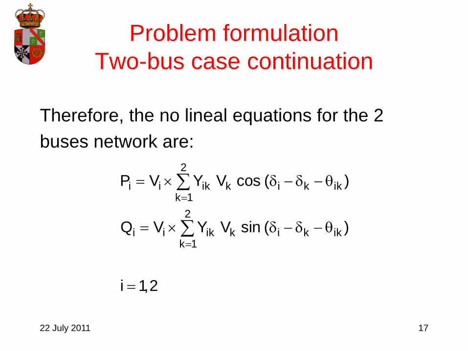
Problem formulation
Two-bus case continuation
Therefore, the no lineal equations for the 2
buses network are:
2,1i
)(sinVYVQ
)(cosVYVP
ikki
2
1kkikii
ikki
2
1kkikii

22 July 2011 18
Problem formulation
Matrix Ybus
• Two bus case
SGS
SSG
2221
1211BUS
YYY
YYY
YY
YYY

22 July 2011 19
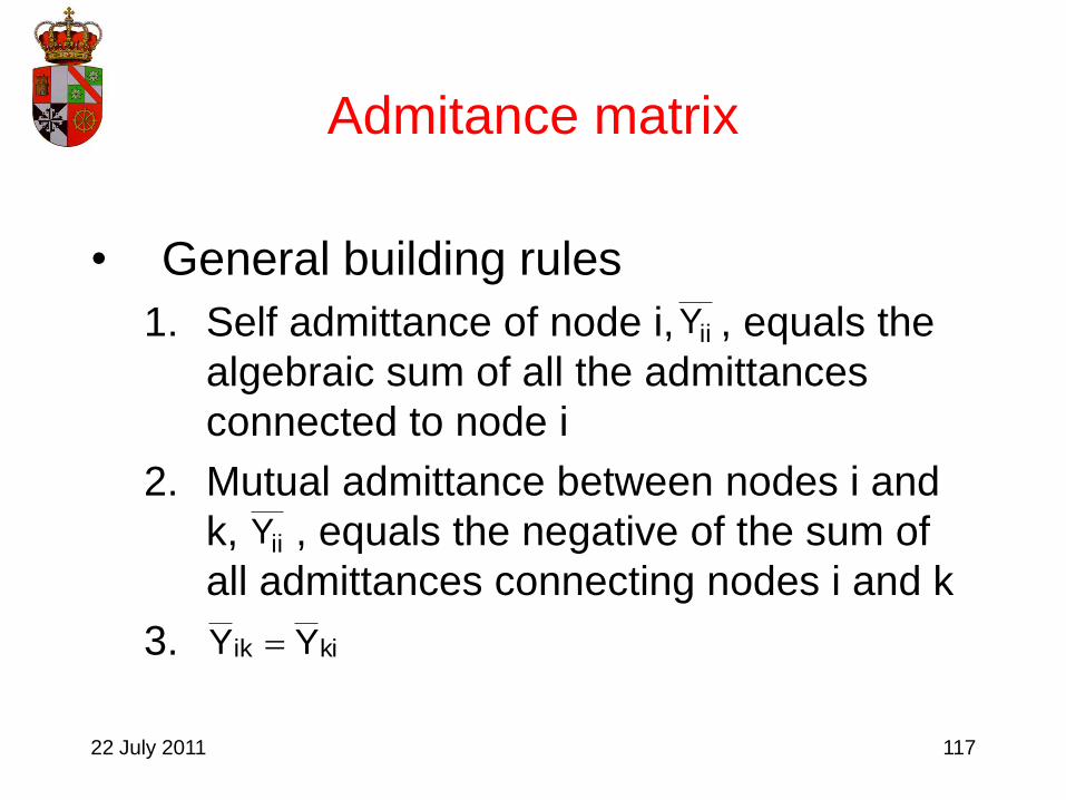
General building rules
Matrix Ybus
1. Self admittance of node i, ,equals the algebraic sum of all the admittances connected to node i
2. Mutual admittance between nodes i and k, ,equals the negative of the sum of all admittances connecting nodes i and k
3.
iiY
ikY
kiYikY

22 July 2011 20
Problem formulation
Matrix Ybus
• Caracteristics of
1. is symmetric
2. is very sparse
(>90% for more than 100 buses)
BUSY
BUSY
BUSY
22 July 2011 21
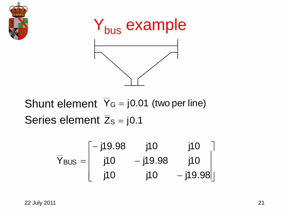
Ybus example
Shunt element
Series element
line) per (two 01.0jYG
1.0jZS
98.19j10j10j
10j98.19j10j
10j10j98.19j
YBUS

22 July 2011 22
Problem formulation
General equations
• 2n equations (static load flow equations)
systembusn
n,...,1i
2)(sinVYVQQQ
1)(cosVYVPPP
ikki
n
1k
kikiDiGii
ikki
n
1k
kikiDiGii

22 July 2011 23
Problem formulation
General equations
kiik
ikikik
ikikikik
n
1kkii
ikikikik
n
1kkii
BjGY
where
]2[)cosBsenG(VVQ
]1[)senBcosG(VVP
Polar representation for voltages and rectangular
for admittances
22 July 2011 24
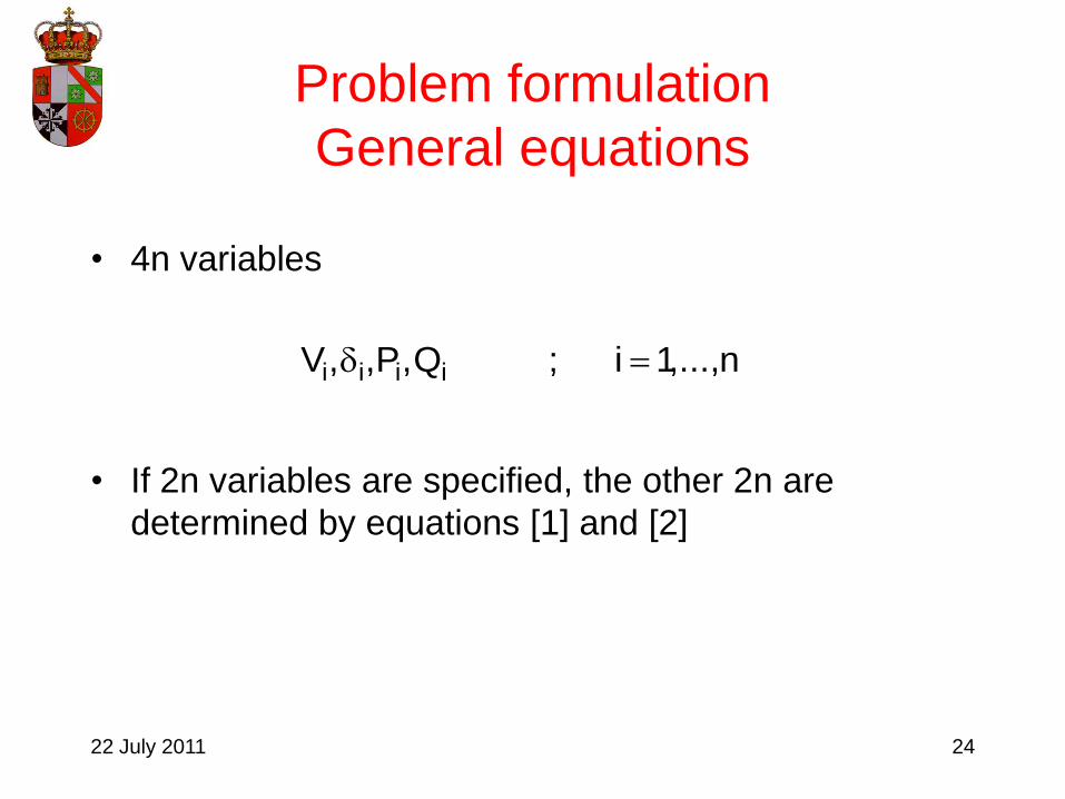
Problem formulation
General equations
• 4n variables
• If 2n variables are specified, the other 2n are
determined by equations [1] and [2]
n,...,1i;Q,P,,V iiii

22 July 2011 25
Problem formulation
BUS Classification
1. PQ buses
known ( known, zero)
known ( known, zero)
unknown
unknown
iP
iQ
iV
i
DiP GiP
DiQ GiQ

22 July 2011 26
Problem formulation
BUS Classification
2. PV buses
known
unknown
known ( specified, known)
known (specified)
unknown ( unknown, known)
unknown
iV
iP
iQ
iP
iQ
DiP
GiQ
GiP
DiQ
i
22 July 2011 27
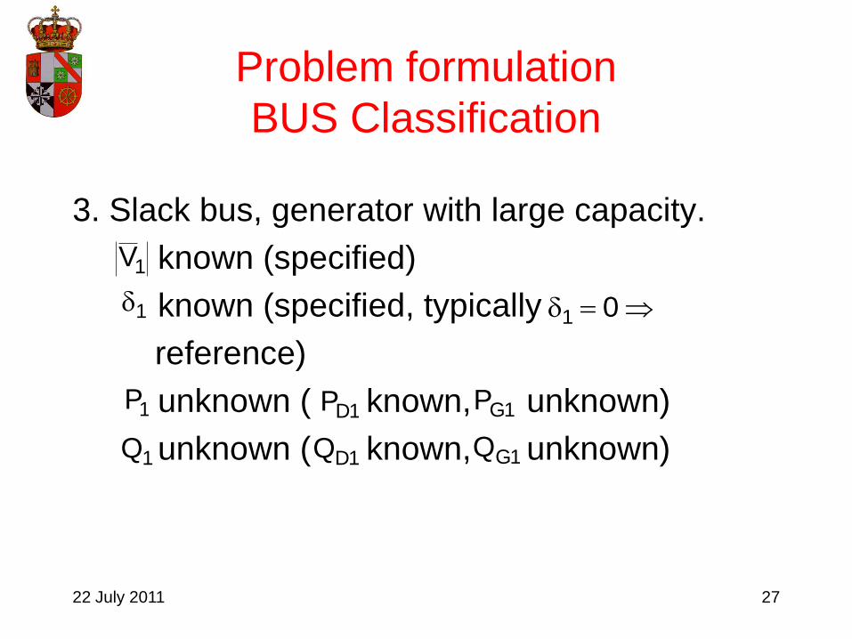
Problem formulation
BUS Classification
3. Slack bus, generator with large capacity.
known (specified)
known (specified, typically
reference)
unknown ( known, unknown)
unknown ( known, unknown)
1V
1
1Q
1P 1DP
1DQ 1GQ
1GP
01

22 July 2011 28
Problem formulation
Variable types and limits
• Power balance
n
1i
n
1iLOSSDiGi
n
1i
n
1iLOSSDiGi
QQQ
PPP
22 July 2011 29
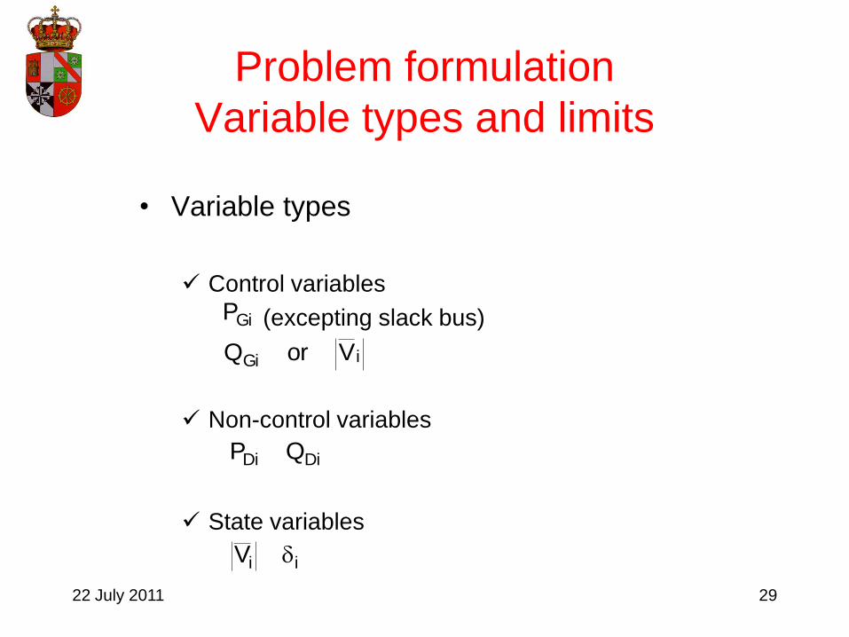
Problem formulation
Variable types and limits
• Variable types
Control variables
(excepting slack bus)
Non-control variables
State variables
GiP
iiV
iGi VorQ
DiDi QP

22 July 2011 30
Problem formulation
Variable types and limits
• Variable limits
Voltage magnitude
Power angle (every existing line)
Power limits
maxiimini VVV
maxkiki
max,GiGimin,Gi
max,GiGimin,Gi
QQQ
PPP

31
3.The Gauss-Seidel solution
technique
22 July 2011

22 July 2011 32
Gauss-Seidel solution technique
)r()1r(
)r()1r(
xx
)x(Fx
)x(Fx0)x(f
No lineal system:
Iteration
Stoping rule

22 July 2011 33
Gauss-Seidel solution technique
Example
Many iterations!
0000.1x,12r
0000.1x,11r
0001.1x,10r
...
0042.1x,6r
0103.1x,5r
...
1442.18.0312.12.0x,2r
312.18.06.12.0x,1r
6.18.022.0x,0r
2x;8.0)x(2.0x
8.0x2.0x
04x5x)x(f
)13(
)12(
)11(
)7(
)6(
2)3(
2)2(
2)1(
)0(2)r()1r(
2
2

22 July 2011 34
Gauss-Seidel solution technique
Algorithm beginning
1) Known
)BusesPV(m,...,2iQ,Q
)BusesPQ(n,...,1miV,V
busslackV
)BusesPV(m,...,2iV
)BusesPQ(n,...,1miQ
)BusesPQ&PV(n,...,2iP
max,Gimin,Gi
maxi
mini
1
i
i
i

22 July 2011 35
Gauss-Seidel solution technique
Algorithm beginning
2) Build
3) Initialize voltages
n,...,2i
n,...,1miVV
0ii
0ii
BUSY

22 July 2011 36
Gauss-Seidel solution technique
PQ buses4) PQ buses
ik;n,...,1k;n,...,1miY
YB
n,...,1miY
jQPA
VYV
jQP
Y
1V
VYVVYVIVjQPS
ii
ikik
ii
iii
n
ik1k
kik*i
ii
iii
n
ik1k
kik*iiii
*ii
*iii
*i

22 July 2011 37
Gauss-Seidel solution technique
PQ buses
At iteration (r+1) and bus i, the available values of
voltages at previous buses are used:
)r(k
n
1ik
ik)1r(
k
1i
1k
ik*)r(
i
i)1r(i VBVB
)V(
AV

22 July 2011 38
Gauss-Seidel solution technique
PV buses
5) PV buses
n
1k
kik*ii
n
1k
kik*ii
*iii
*i
VYVQ
VYVIVjQPS

22 July 2011 39
Gauss-Seidel solution technique
PV buses
At iteration (r+1):
1i
1k
n
1ik
)r(
kik)1r(
kik*)r(
i
)1r(
i)1r(i
ii
)1r(ii)1r(
iii
n
ik
)r(
kik
1i
1k
*)r(
i
)1r(
kik*)r(
i)1r(
i
VBVB)V(
Aangle
Y
jQPAVangle
VY)V(VY)V(Q
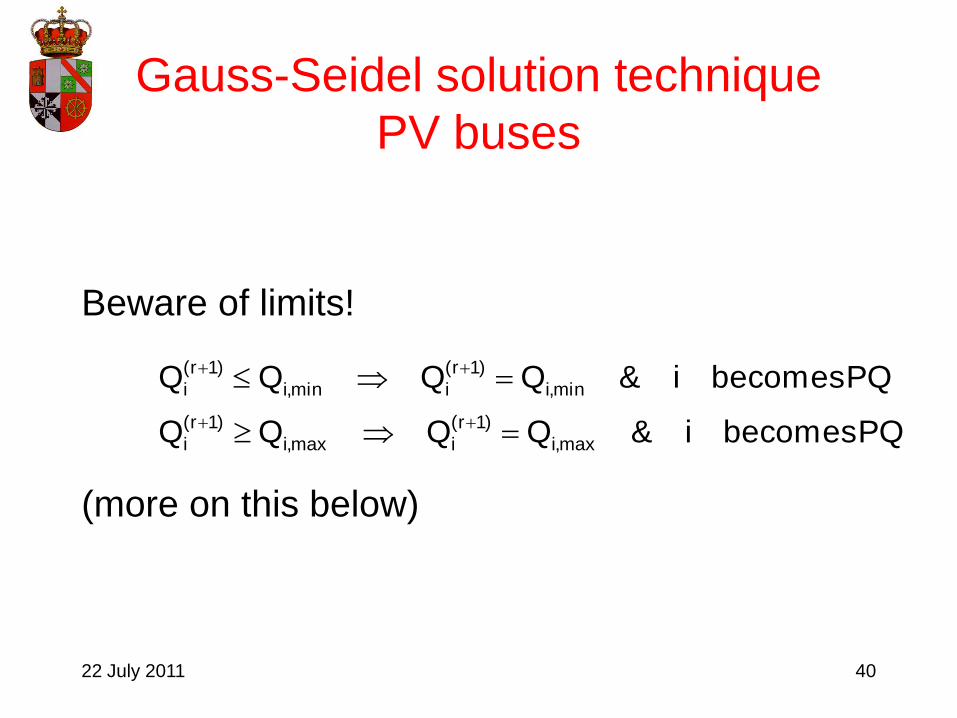
22 July 2011 40
Gauss-Seidel solution technique
PV buses
Beware of limits!
PQbecomesi&QQQQ
PQbecomesi&QQQQ
max,i
)1r(
imax,i
)1r(
i
min,i
)1r(
imin,i
)1r(
i

22 July 2011 41
Gauss-Seidel solution technique
PV buses
6.1) Slack bus power (after convergence)
n
1k
kk1*111
)r(i
)1r(i
VYVjQP
n,...,2i;VV
6) Stop criterion
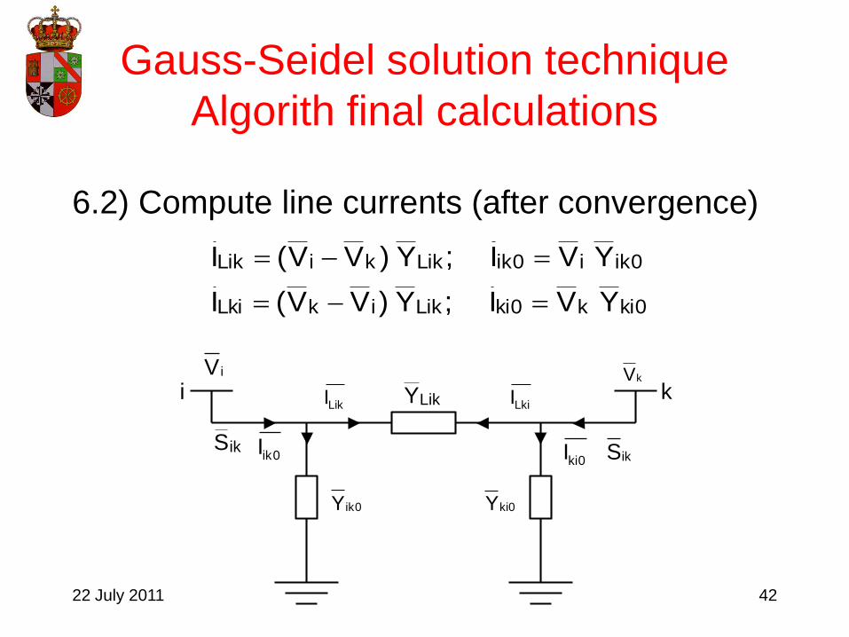
22 July 2011 42
Gauss-Seidel solution technique
Algorith final calculations
6.2) Compute line currents (after convergence)
iV
ikV
k
ikSikS
0ikY
LikY
0ikI
LikI LkiI
0kiY
0kiI
0kik0kiLikikLki
0iki0ikLikkiLik
YVI;Y)VV(I
YVI;Y)VV(I

22 July 2011 43
Gauss-Seidel solution technique
Algorith final calculations6.2) Compute line complex power (after convergence)
;YVVY)VV(VS
;YVVY)VV(VS
*0ik
*ii
*Lik
*k
*iiik
*0ki
*kk
*Lik
*i
*kkki
iV
ikV
k
ikSikS
0ikY
LikY
0ikI
LikI LkiI
0kiY
0kiI
22 July 2011 44
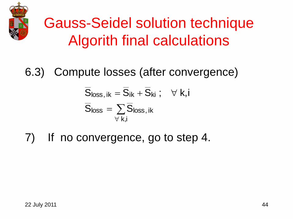
Gauss-Seidel solution technique
Algorith final calculations
6.3) Compute losses (after convergence)
7) If no convergence, go to step 4.
i,k
ik,lossloss
kiikik,loss
SS
i,k;SSS

22 July 2011 45
Gauss-Seidel solution technique
Algorithm improvement
• Acceleration factor (in order to decrease
the number of iterations):
)r(
i
)1r(
i
)r(
i)1r(
i VVVV~
1.6 (generally recommended)

22 July 2011 46
Gauss-SeidelMatlab code
function [Vfinal,angfinal,nite,P,Q,errorplot,tiempo]=Gaussgen(m,n,Ybus,Vmodini,Angini,P,Q,tol,Vmax,Vmin,Qmax,Qmin)
%--------------------------------------------------------------------------------------------------------------------------------------------------
%-function [Vmod,ang,nite,P,Qerrorplot,tiempo]=Gaussgen(m,n,Ybus,Vmodini,Angini,P,Q,tol,Vmax,Vmin,Qmax,Qmin)
%-Resuelve de forma general problema de carga por el m´etodo de Gauss-Seidel
%-donde:
%-2...m nudos PV; (m=1 cuando no hay nudos PV)
%-n nudos totales
%-Ybus matriz de admitancias
%-Vmodini tensiones iniciales modulo
%-Angini angulos iniciales RADIANES
%-P potencia activa inicial
%-Q potencia reactiva inicial
%-tol tolerancia para error en tension y potencia reactiva
%-Vmax Vmin valores limites aceptables para las tensiones
%-Qmax Qmin valores limites aceptables para las potencias reactivas
%-nite n´umero de iteraciones
%-Vfinal vector con todas las potencias para cada iteraci´on
%-angfinal igual pero con los ´angulos
%-tiempo, tiempo invertido en hacer las operaciones
%---------------------------------------------------------------------------------------------------------------------------------------------------
%calculo de la matriz B
B=zeros(n,n);
for t=1:n
for k=1:n
B(t,k)=Ybus(t,k)/Ybus(t,t);
end
end

22 July 2011 47
Gauss-SeidelMatlab code 2
%calculos los valores en coordenadas cuadrangulares de la tension
V=zeros(n,1);
for a=1:n
V(a)=Vmodini(a)*exp(i*Angini(a));
end
ang=Angini;
%empieza el bucle:
error=1; %valores iniciales para poder entrar en el bucle
errorQ=1;
nite=0;
tic;
while max(abs(error))>tol | max(abs(errorQ))>tol
nite=nite+1;
Vmod=abs(V);
Vini=V;
ang=angle(V);
Qini=Q;
%calculo las reactivas para los nudos PV
if m>1
for l=2:m
AQ=0;
for k=1:n
AQ=AQ+Ybus(l,k)*V(k);
end
Q(l)=-imag((V(l)')*AQ);
end

22 July 2011 48
Gauss-SeidelMatlab code 3
%calculo las A para todos los nudos:
for a=1:n
A(a)=(P(a)-i*Q(a))/Ybus(a,a);
end
%calculo los angulos nudos PV:
for l=2:m
Aang=0;
for k=1:n
Aang=Aang+B(l,k)*V(k);
end
ang(l)=angle(A(l)/((V(2))')-Aang+B(l,l)*V(l));
end
end
for a=1:n
A(a)=(P(a)-i*Q(a))/Ybus(a,a);
end
%ahora actualizo los voltajes otra vez:
for a=1:n
V(a)=Vmod(a)*exp(i*ang(a));
end
%ahora calculo los nudos PQ
AV=zeros(n,1);
for p=m+1:n
for k=1:n
AV(p)=AV(p)+B(p,k)*V(k);
end
V(p)=A(p)/((V(p))')-AV(p)+B(p,p)*V(p);
end
error=Vini-V;
errorQ=Qini-Q;
errorplot(1,nite)=norm(abs(error));
Vfinal(:,nite)=abs(V);
angfinal(:,nite)=ang*180/pi; %paso a grados
end

22 July 2011 49
Gauss-SeidelMatlab code 4
%calculos los valores de potencia para el nudo slack:
S1=0;
for t=1:n
S1=S1+(V(1)')*(Ybus(1,t)*V(t));
end
P(1)=real(S1);
Q(1)=-imag(S1);
tiempo=toc;
%alerta por si se sobrepasan valores aceptables:
if max(Vmod)>Vmax | min(Vmod)<Vmin
disp('¡¡SE SOBREPASAN LIMITES TENSIONES!!')
end
if max(Q)>Qmax | min(Q)<Qmin
disp('¡¡SE SOBREPASAN LIMITES REACTIVA!!')
end
ang=(180/pi)*angle(V);
Vmo=abs(V);
%represento los errores por iteraci´on:
plot(1:nite,errorplot,'o');grid on;xlabel('iteraci´on');ylabel('error por iteraci´on');title('evoluci´on error tesi´on');
%------------------------------------------------------------%
% %
% Realizado por Carlos Ruiz Mora octubre 2006 %
% %
%------------------------------------------------------------%

50
Gauss-Seidel example
22 July 2011

22 July 2011 51
G-S Example
Solution tolerance is set to 0.1 MVA.
ONE TWO
THREE

22 July 2011 52
G-S Example
Data below. Base power is SB=100 MVA:
Bus Voltage (p.u.) Power
1 1.02 (slack)
2 1.02 PG=50 MW
3 - PC=100 MW
QC=60 MVAr
Lin Impedance (p.u.)
1-2 0.02+0.04j
1-3 0.02+0.06j
2-3 0.02+0.04j
(each)

22 July 2011 53
Solution procedure
1. Data and unknown:
Bus Type Data Unknown
1 Slack V1=1.02 1=0.0 P1 Q1
2 PV V2=1.02 P2=0.5 δ2 Q2
3 PQ P3=-1.0 Q2=-0.6 δ3 V3
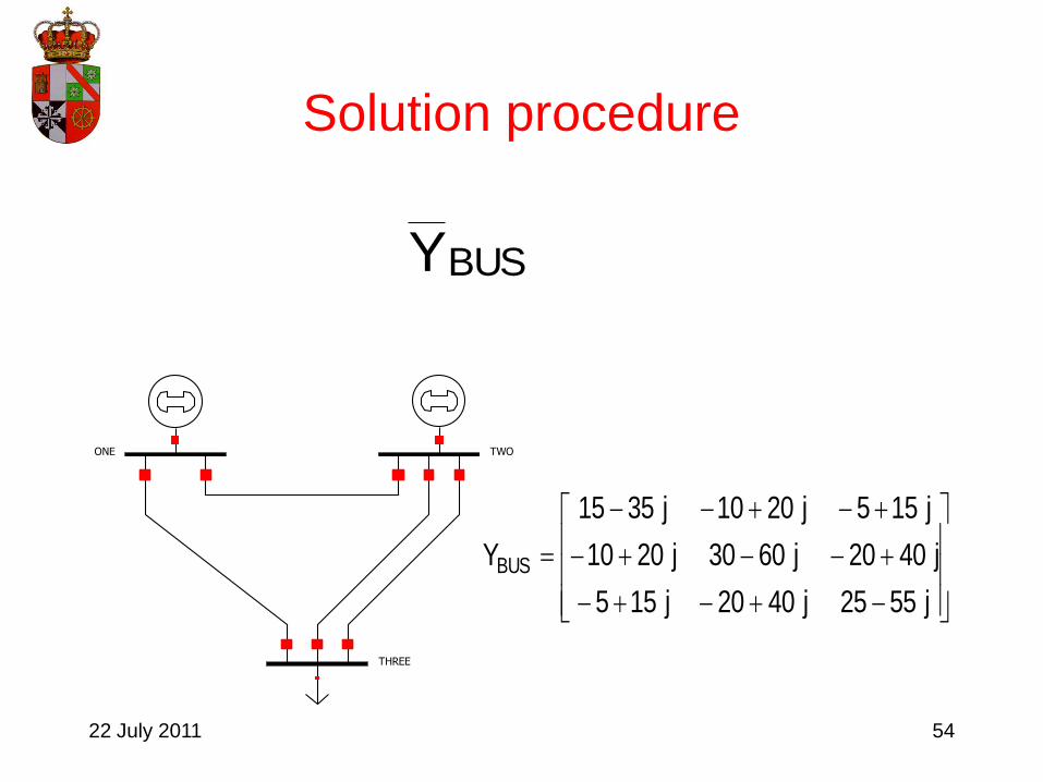
22 July 2011 54
Solution procedure
j5525j4020j155
j4020j6030j2010
j155j2010j3515
YBUS
BUSY
ONE TWO
THREE
22 July 2011 55
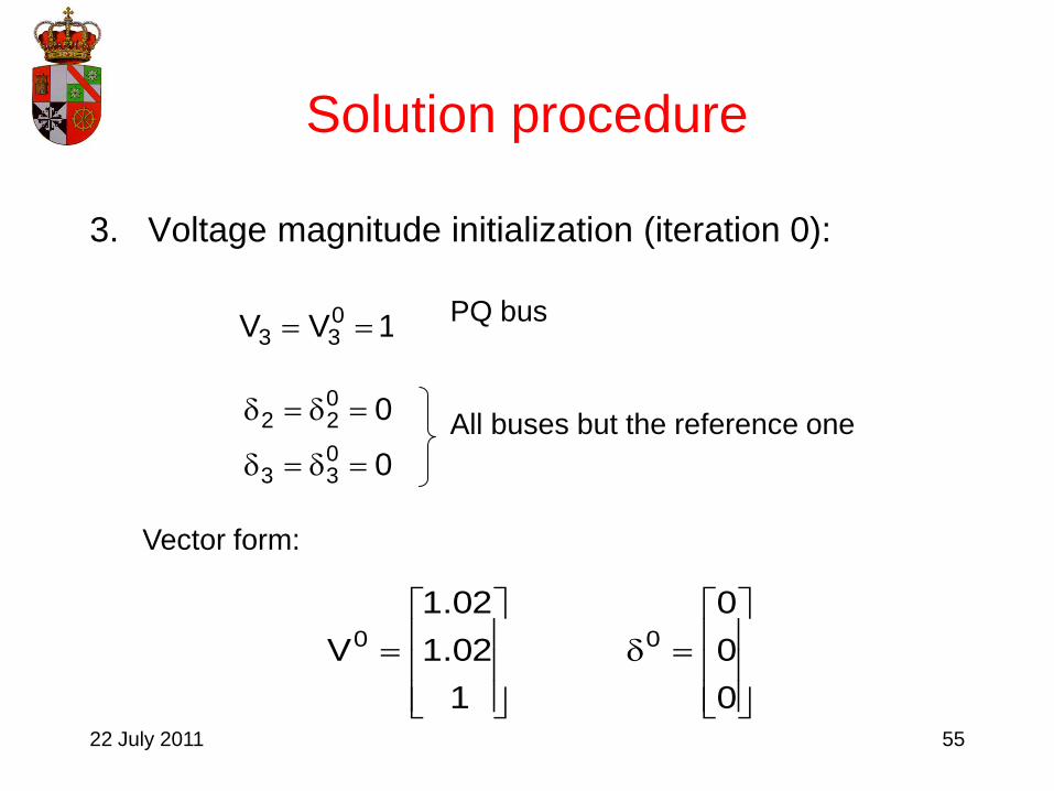
Solution procedure
3. Voltage magnitude initialization (iteration 0):
1VV 033
PQ bus
0
0
033
022
All buses but the reference one
Vector form:
0
0
0
1
02.1
02.1
V 00

22 July 2011 56
Solution procedure
Per iteration:
- PV buses (Q, δ) i=2,...,m (bus 2)
- PQ buses (V, δ) i=m+1,...,n (bus 3)
- Stopping criterios:
a) convergence Sslack and power flows;
b) no converge new iteration

22 July 2011 57
Solution procedure
4. PV buses: iteration (r+1) :
bus 2:
22
)1r(
22)1r(
222
)r(
323
*)r(
2
)r(
222
*)r(
2
)1r(
121
*)r(
2
)1r(
2
Y
jQPA]V[ angle
VY)V(VY)V(VY)V(Q

22 July 2011 58
Solution procedure
)r(
323
)1r(
121*)1r(
2
)1r(
2)1r(
2 VBVB)V(
Aangle
where
ii
ikik
Y
YB is a constant

22 July 2011 59
Solution procedure
5. Buses PQ iteration (r+1):
bus 3:
)1r(232
)1r(131*)r(
3
3)1r(3 VBVB
)V(
AV
where
ii
ikik
33
333
Y
YB
Y
jQPA
Are constants for PQ buses

22 July 2011 60
Solution procedure
6. Stopping criterion:
310
|QQ|
&
|VV|
)r(j
)1r(j
)r(i
)1r(i
2j ;3 ,2i

22 July 2011 61
Solution procedure
If convergence:
6.1) Slack power
6.2) Power flows
)VYVYVY(VjQPS 313212111*111
*slack
*Likk
*iiik Y)VV(VS -*
323123132112 S,S,S,S,S,S

22 July 2011 62
Solution procedure
6.3) Line losses:
23,loss13,loss12,lossloss
kiikik,losss
SSSS
3,2,1i,kSSS
7. If no coveergence, the procedure continues in Step 4.

22 July 2011 63
Implementation
MATLAB:

22 July 2011 64
Solution
11 iterations needed to attain the solution
Iteration (pu) 1 2 3 ... 10 11
P1 ,Q1(slack) - - - ... -0.5083
0.0716
P2 0.5 0.5 0.5 ... 0.5 0.5
Q20.81 0.4084 0.4696 ... 0.5493 0.5501
P3-1.0 -1.0 -1.0 ... -1.0 -1.0
Q3-0.6 -0.6 -0.6 ... -0.6 -0.6

22 July 2011 65
Solution
Iteration 1 2 3 ... 10 11
1.02 1.02 1.02 ... 1.02 1.02
0 0 0 ... 0 0
1.02 1.02 1.02 ... 1.02 1.02
0.0675 -0.1596 -0.2885 ... -0.4667 -0.4685
1.0041 1.0042 1.0043 ... 1.0043 1.0043
-0.5746 -0.7336 -0.8278 ... -0.9580 -0.9593
1V
2V
3V
)(º1
)(º2
)(º3

22 July 2011 66
Solution
Iteration 1 2 3 ... 10 11
Max. Error V 0.0041 9.68·10-5 5.05·10-5 ... 1.15·10-6 6.74·10-7
Max. Error Q 0.8160 0.4076 0.0612 ... 0.0014 8.11·10-4
Errors for |V| & |Q|:

22 July 2011 67
Final Solution
Bus P (MW) Q (MVAr ) (pu)
1 50.83 7.16 1.02 0º
2 50.00 55.01 1.02 -0.4685º
3 -100 -60.00 1.0043 -0.9593º
V

22 July 2011 68
Checking
Checking using Power-World:
ONE TWO
THREE

22 July 2011 69
Checking
Bus 1 Bus 2 Bus 3
Solution G-S PW G-S PW G-S PW
V (pu) 1.02 1.02 1.02 1.02 1.0043 1.0043
δ(º) 0 0 -0.4685 -0.4710 -0.9593 -0.9612
P (MW) 50.83 50.98 50.00 50.00 -100 -100
Q (MVAr) 7.16 7.10 55.01 55.12 -60 -60

22 July 2011 70
Checking
Variable V δ P Q
Error Max. (%) 0 % 0.53 % 0.29% 0.84 %

71
4. The Newton-Raphson solution
technique
22 July 2011

22 July 2011 72
The Newton-Raphson solution technique
Introduction
• One variable
)r(
)r()r()1r(
)0()0()1(
)0(
)0()0(
)0()0()0()0()0(
)0()0()0(
dx
df
)x(fxx
xxx;
dx
df
)x(fx
...dx
dfx)x(f0)xx(f
0)xx(f,0)x(f,0)x(f

22 July 2011 73
The Newton-Raphson solution technique
Introduction
• Example
!Fast
0000.159988.02
49988.059988.09988.0x
9988.059375.02
49375.059375.09375.0x
9375.055.02
45.055.05.0x
5.0x;5x2
4x5)x(xx
5x2dx
)x(df;04x5x)x(f
2)3(
2)2(
2)1(
)0(
)r(
)r(2)r()r()1r(
2
22 July 2011 74
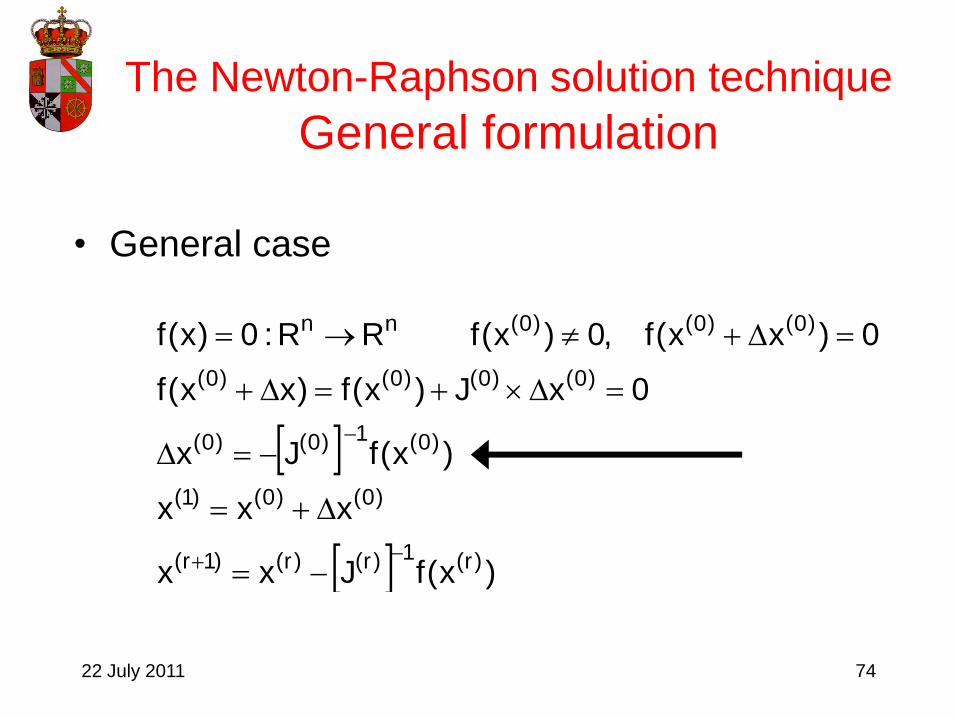
The Newton-Raphson solution technique
General formulation
• General case
)x(fJxx
xxx
)x(fJx
0xJ)x(f)xx(f
0)xx(f,0)x(fRR:0)x(f
)r(1)r()r()1r(
)0()0()1(
)0(1)0()0(
)0()0()0()0(
)0()0()0(nn

22 July 2011 75
The Newton-Raphson solution technique
General formulation
n
n
2
n
1
n
n
2
2
2
1
2
n
1
2
1
1
1
n
2
1
n
2
1
x
f
x
f
x
f
x
f
x
f
x
f
x
f
x
f
x
f
J
f
f
f
f
x
x
x
x
22 July 2011 76
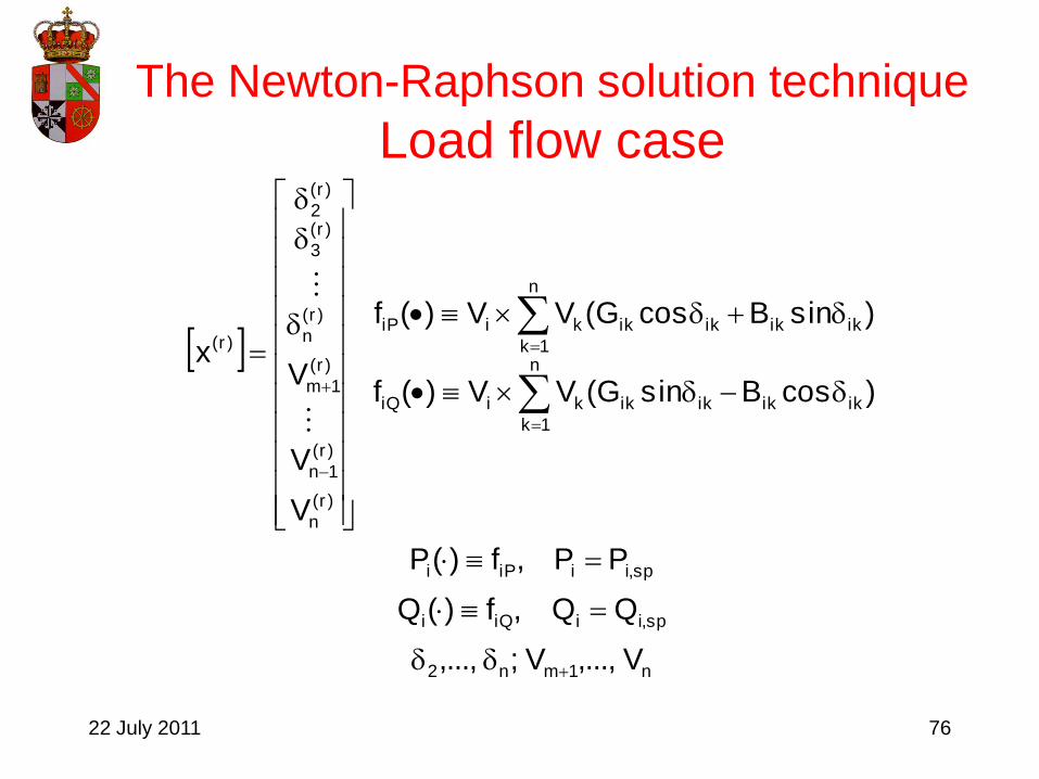
The Newton-Raphson solution technique
Load flow case
n1mn2
sp,iiiQi
sp,iiiPi
n
1k
ikikikikkiiQ
n
1k
ikikikikkiiP
)r(
n
)r(
1n
)r(
1m
)r(
n
)r(
3
)r(
2
)r(
V,...,V;,...,
QQ,f)(Q
PP,f)(P
)cosBsinG(VV)(f
)sinBcosG(VV)(f
V
V
Vx

22 July 2011 77
The Newton-Raphson solution technique
Load flow case
)r(
iQsp,i
)r(
i
)r(
iPsp,i
)r(
i
)r(
n
)r(
n
iQ)r(
1m
)r(
1m
iQ)r(
n
)r(
n
iQ)r(
2
)r(
2
iQ)r(
iQsp,i
)r(
n
)r(
n
iP)r(
1m
)r(
1m
iP)r(
n
)r(
n
iP)r(
2
)r(
2
iP)r(
iPsp,i
fQQ;fPP
VV
f...V
V
ff...
ffQ
VV
f...V
V
ff...
ffP
Using Taylor:
The increments below should be 0:
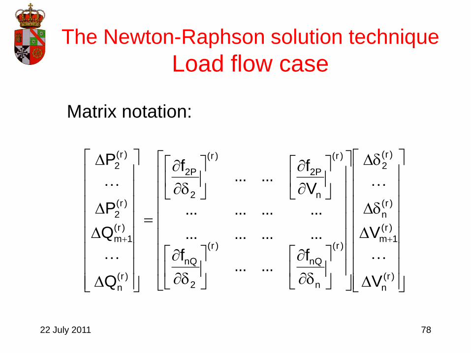
22 July 2011 78
The Newton-Raphson solution technique
Load flow case
)r(
n
)r(
1m
)r(
n
)r(
2
)r(
n
nQ
)r(
2
nQ
)r(
n
P2
)r(
2
P2
)r(
n
)r(
1m
)r(
2
)r(
2
V
V
f......
f
............
............
V
f......
f
Q
Q
P
P
Matrix notation:
22 July 2011 79
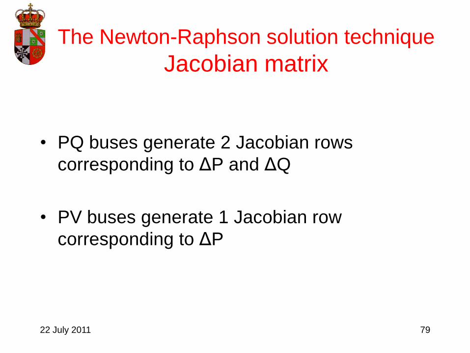
The Newton-Raphson solution technique
Jacobian matrix
• PQ buses generate 2 Jacobian rows
corresponding to ΔP and ΔQ
• PV buses generate 1 Jacobian row
corresponding to ΔP
22 July 2011 80
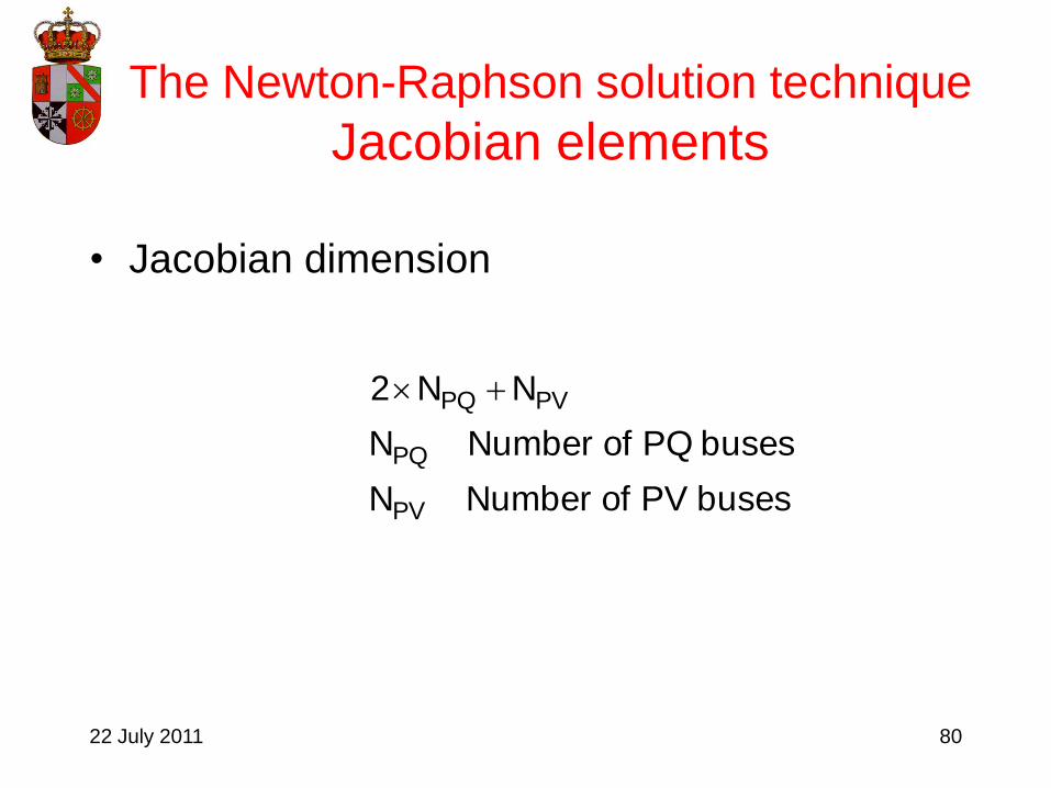
The Newton-Raphson solution technique
Jacobian elements
• Jacobian dimension
busesPVofNumberN
busesPQofNumberN
NN2
PV
PQ
PVPQ

22 July 2011 81
The Newton-Raphson solution technique
Jacobian elements
• Jacobian dimension
efficiencynalcomputatioimprovingfor
VofinsteadV
V
VV
LJ
NH
Q
P
)1r(
)r(
)1r(
)r(
)1r(
)1r(
)r()r(
)r()r(
)r(
)r(

22 July 2011 82
The Newton-Raphson solution technique
Jacobian elements
)cosBsinG(VVV
QVL
)sinBcosG(VVQ
J
)sinBcosG(VVV
PVN
)cosBsinG(VVP
H
km
kmkmkmkmmk
m
kmkm
kmkmkmkmmk
m
kkm
kmkmkmkmmk
m
kmkm
kmkmkmkmmk
m
kkm

22 July 2011 83
The Newton-Raphson solution technique
Jacobian elements
2kkkk
k
kkkk
kmkmkm2kkkk
k
kkk
mkkm2kkkk
k
kkkk
2kkkk
k
kkk
VBQV
QVL
jBGYVGPQ
J
VGPV
PVN
:NoteVBQP
H
mk

22 July 2011 84
The Newton-Raphson solution technique
Solution outline
1. Build
2. Specify
3. Initialize
1
i
i
i
1
V
m,...,2iV
n,...,1miQ
n,...,2iP
0
n,...,1mi,V
n,...,2i,
i
i
BUSY

22 July 2011 85
The Newton-Raphson solution technique
Solution outline
4. Compute
5. If
6. Compute submatrices
ongoelse
Stop)3
flowsline)2
jQP)1
computethen
Q&P
11
Q)r(
iP)r(
i
)r()r()r()r( L,J,N,H
)BusesPQfor(Q),BusesPQ&PVfor(P )r(i
)r(i

22 July 2011 86
The Newton-Raphson solution technique
Solution outline
7. Solve
8. Update
9. Go to step 4
)r(
)r(1
)r()r(
)r()r(
)r(
)1r(
)1r(
Q
P
LJ
NH
VV
BusesPVVVV
BusesPQ&PV
)1r()r()1r(
)1r()r()1r(

22 July 2011 87
The Newton-Raphson, Matlab Code
function [V_modulo, V_fase, P, Q, N_iter, T_calculo, Error_p] = nraphson(V_modulo_ini, V_fase_ini, P_ini, Q_ini, Y, npv)
%
% [V_modulo, V_fase, P, Q, N_iter, T_calculo, Error_p] = nraphson(V_modulo_ini, V_fase_ini, P_ini, Q_ini, Y, npv)
%
% Obtencion de indices de nodos: 1 -> SLACK;
% 2,...,M -> PV;
% M+1,...,N -> PQ
n = length(V_modulo_ini);
m = npv + 1;
% Parametros del Metodo
Tol = 0.0001; % Tolerancia del metodo (Perdida de potencia).
Error_p = 1; % Error inicial (A un valor mayor que Tol).
N_iter = 0; % Numero de iteraciones.
% Valores iniciales
V_modulo= V_modulo_ini';
V_fase = V_fase_ini';
P = P_ini';
Q = Q_ini';
j=sqrt(-1);

22 July 2011 88
The Newton-Raphson, Matlab Code
tic;
while (Error_p > Tol) % Bucle principal (Se permiten 50 iteraciones como mucho).
if (N_iter >50)
error('Demasiadas iteraciones');
break
end
V = V_modulo.*exp(j*V_fase); % Expresion compleja de la tension
S = V.*conj(Y*V); % Expresion compleja de la potencia
DP = P(2:n)-real(S(2:n)); % Incremento de potencia activa (nudos PV y PQ)
DQ = Q(m+1:n)-imag(S(m+1:n)); % Incremento de potencia reactiva (nudos PQ)
PQ = [DP ; DQ];
Error_p = norm(PQ,2); % Error en esa iteracion
DS_DA = diag(V)*conj(Y*j*diag(V)) + diag(conj(Y*V))*j*diag(V);
DS_DV = diag(V)*conj(Y*diag(V./V_modulo)) + diag(conj(Y*V))*diag(V./V_modulo);
% Construccion del Jacobiano
J = [real(DS_DA(2:n , 2:n)) real(DS_DV(2:n , m+1:n))
imag(DS_DA(m+1:n , 2:n)) imag(DS_DV(m+1:n , m+1:n))]
dx=J\PQ; % indices: 1...n-1 = fases en PV y PQ; n...final = modulos en PQ

22 July 2011 89
The Newton-Raphson, Matlab Code
V_fase (2:n) = V_fase(2:n) + dx(1:n-1); % Actualizamos la fase de las tensiones (nudos PV y PQ)
V_modulo (m+1:n)= V_modulo(m+1:n) + dx(n:end); % Actualizamos el modulo de las tensiones (nudos PQ)
N_iter = N_iter + 1; % Incremento el numero de iteraciones
disp('Pulse una tecla para continuar')
pause
end
P=real(S); % Calculo de la potencia activa
Q=imag(S); % Calculo de la potencia reactiva
V_fase=V_fase*180/pi; % Paso de Radianes a grados
T_calculo=toc;
% **** ENTRADAS ****
%
% V_modulo_ini = Modulo de la tension para comenzar a iterar (conocidos en SLACK y PV).
% V_fase_ini = Fase de la tension para comenzar a iterar (conocido en SLACK).
% P_ini = Potencia activa en los nodos (conocido en PV y PQ).
% Q_ini = Potencia reactica en los nodos (conocido en PQ).
% Y = Matriz de admitancias nodales.

22 July 2011 90
The Newton-Raphson, Matlab Code
% **** SALIDAS ****
%
% V_modulo = Modulo de la tension en todos los nodos.
% V_fase = Fase de la tension en todos los nodos.
% P = Potencia activa en todos los nodos.
% Q = Potencia reactiva en todos los nodos.
% N_iter = Numero de iteraciones.
% T_calculo = Tiempo de calculo.
% Error_p = Error.
%
%
% **** OBSERVACIONES ****
%
% Los nodos deben estar ordenador asi:
%
% * 1 : SLACK.
% * 2...m : PV.
% * m+1...n : PQ.
%
%
% **** FECHA Y AUTOR ****
%
% Laura Laguna - Octubre de 2005

22 July 2011 91
Ejemplo resuelto por el método
de Newton-Raphson

22 July 2011 92
Newton-Raphson Example
• Checking with Matlab and PowerWorld

22 July 2011 93
Newton-Raphson Example
Bus Voltage p.u Power
1 1.02 -
2 1.02 PG=50 MW
3 - PC= 100 MW
QC=60 MVAr
ONE TWO
THREE

22 July 2011 94
Newton-Raphson Example
Data:
Line Impedance p.u.
1-2 0.02+0.04j
1-3 0.02+0.06j
2-3 0.02+0.04j each

22 July 2011 95
Newton-Raphson Example
• 3 buses:
• Bus1: Slack
• Bus 2: PV
• Bus 3: PQ
• Voltage magnitude at bus 3 initialized at 1.02.
• Angles intitialized to zero.

22 July 2011 96
Newton-Raphson Example
Y bus:
55.0000j- 25.000040.0000j+ 20.0000-15.0000j+ 5.0000-
40.0000j+ 20.0000-60.0000j- 30.000020.0000j+ 10.0000-
15.0000j+ 5.0000-20.0000j+ 10.0000-35.0000j- 15.0000
Y
Intitialization:
02.1V
0
3
32

22 July 2011 97
Newton-Raphson Example
Residuals:
3i))cos(BsenG(VVQQ
3,2i))(senBcosG(VVPP
3
1j
ijijijijji
esp
ii
3
1j
ijijijijji
esp
ii
∑
∑
--
-
22 July 2011 98
Newton-Raphson Example
Checking:
No tolerance satisfied: the process continues.
6.0
1
5.0
Q6.0
P1
P5.0
Q
P
P
10·2475.7
0
10·3624.0
Q
P
P
cal
3
cal
3
cal
2
3
3
2
15
14
cal
3
cal
3
cal
2

22 July 2011 99
Newton-Raphson Example
Jacobian:
333332
333332
232322
LMM
NHH
NHH
J
1000.560100.268080.20
5000.252220.576160.41
4000.206160.414240.62
J

22 July 2011 100
Newton-Raphson Example
First iteration:
0.0154-
0.9406-
0.4557-
VV
3
3
3
2
0.9406-
0.4557-
0
;
0046.1
0200.1
0200.1
V

22 July 2011 101
Ejemplo por Newton-Raphson
Residuals:
No convergence.
0126.0
0165.0
0042.0
)5874.0(6.0
)9835.0(1
4958.05.0
Q
P
P
5874.0
9835.0
4958.0
Q
P
P
3
3
2
cal
3
cal
3
cal
2

22 July 2011 102
Newton-Raphson Example
Jacobian for iteration 2:
6707.542162.268409.20
1371.240994.568145.40
0540.201614.418860.61
J

22 July 2011 103
Newton-Raphson Example
State variables at iteration 2
4-
3
3
3
2
3.0024·10-
0.0206-
0.0154-
VV
0.9612-
0.4710-
0
;
0043.1
0200.1
0200.1
V

22 July 2011 104
Newton-Raphson Example
Residuals:
Tolerance OK.
6
5
5
3
3
2
cal
3
cal
3
cal
2
10·9698.4
10·5454.0
10·0664.0
)6000.0(6.0
)0000.1(1
5000.05.0
Q
P
P
6000.0
0000.1
5000.0
Q
P
P
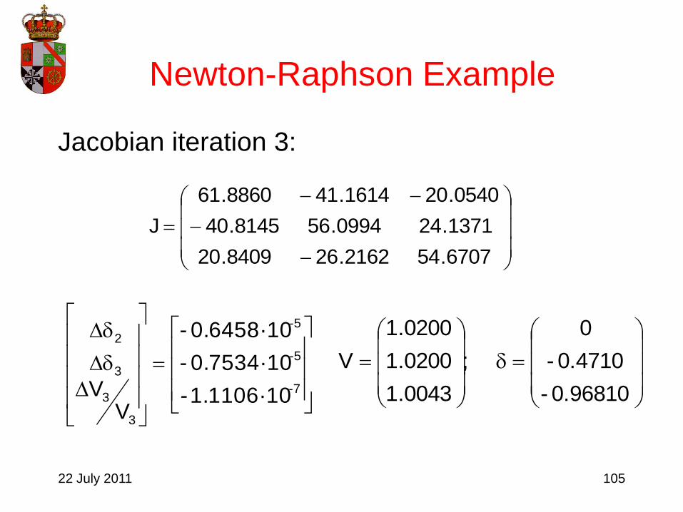
22 July 2011 105
Newton-Raphson Example
0.96810-
0.4710-
0
;
0043.1
0200.1
0200.1
V
7-
5-
5-
3
3
3
2
1.1106·10-
0.7534·10-
0.6458·10-
VV
Jacobian iteration 3:
6707.542162.268409.20
1371.240994.568145.40
0540.201614.418860.61
J

22 July 2011 106
Newton-Raphson Example
Final power values:
6000.0
5513.0
0710.0
Q
Q
Q
0000.1
5000.0
5098.0
P
P
P
3
2
1
3
2
1
22 July 2011 107
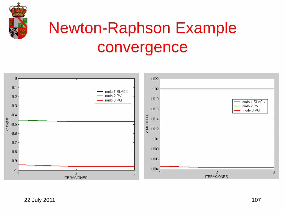
Newton-Raphson Example
convergence

22 July 2011 108
Newton-Raphson Exampleconvergence
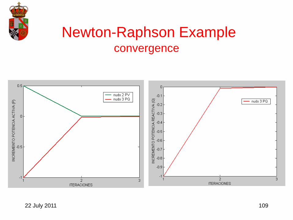
22 July 2011 109
Newton-Raphson Exampleconvergence

22 July 2011 110
Newton-Raphson Exampleconvergence
22 July 2011 111
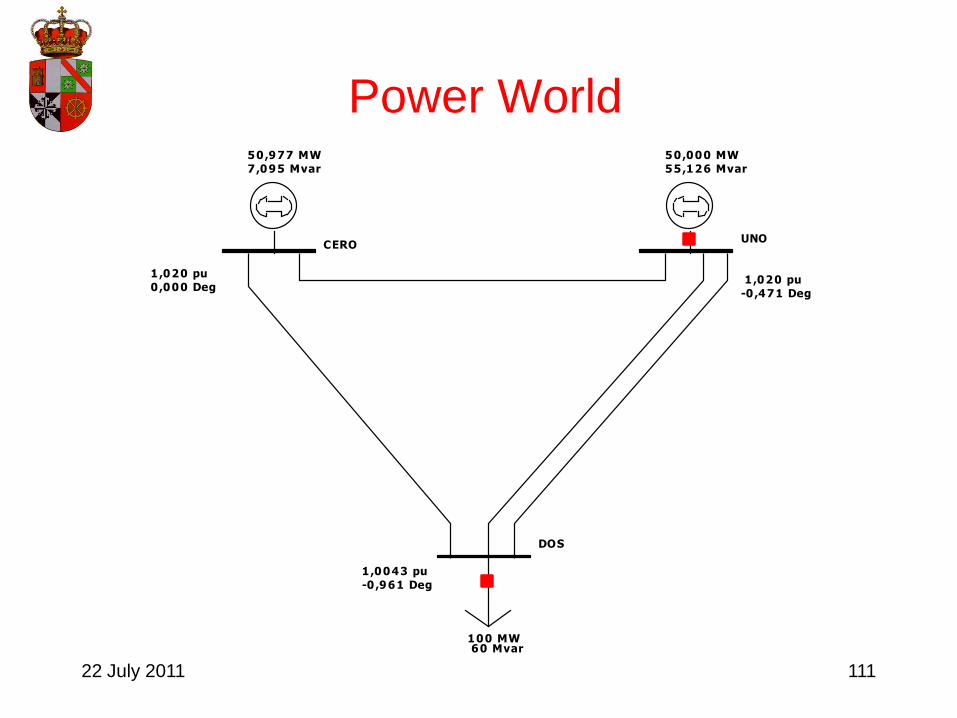
Power World
CEROUNO
DOS
50,977 MW
7,095 Mvar
50,000 MW
55,126 Mvar
100 MW 60 Mvar
1 ,020 pu
0 ,000 Deg 1 ,020 pu
-0 ,471 Deg
1,0043 pu
-0 ,961 Deg

22 July 2011 112
Newton-Raphson Example
Bus V(p.u) δ P Q
0 (PW) 1.02 0 50.9763 7.0955
0 1.02 0 50.9755 7.0954
1 (PW) 1.02 -0.4710 50 55.1256
1 1.02 -0.4710 50.0006 55.1228
2 (PW) 1.0043 -0.9612 -100 -60
2 1.0043 -0.9612 -99.9989 -59.9970

22 July 2011 113
Newton-Raphson Example
• Largest error below 0.1 MVA.
• More effective technique than Gauss Seidel.
• Convergence is fast (if adequate initialization).

22 July 2011 114
Including tap-changing transformers

22 July 2011 115
Tap-Changing transformer
• A tap changing transformer makes the
admitance matrix dependent on the
transformer parameter t.
• The Jacobian matrix also depends on t.

22 July 2011 116
Admitance matrix
Equivalent circuit:
i jt:1
ccY tYcc
2cct
t1Y
t
1tYcc
ji
1t
22 July 2011 117
Admitance matrix
• General building rules
1. Self admittance of node i, , equals the
algebraic sum of all the admittances
connected to node i
2. Mutual admittance between nodes i and
k, , equals the negative of the sum of
all admittances connecting nodes i and k
3.
iiY
iiY
kiik YY

22 July 2011 118
Tap-changing
Example

22 July 2011 119
Tap-changing
Example
tYcc
2cct
t1Y
t
1tYcc
1 3 2
4
13Z 23Z
13shuntY23shuntY
13shuntY23shuntY
The tap-changing
transformer
controls voltage
of bus 4

22 July 2011 120
Tap-changing
Example
cccccc
44
cc34
cc2cc23shunt
2313shunt
1333
1213shunt13
11
Yt
1tY
tY
Y
tY
Y
tY
t
t1YY
Z
1Y
Z
1Y...
...;0Y;YZ
1Y
It does not depend
on t!

22 July 2011 121
Tap-changing
Example
44434241
34333231
24232221
14131211
Y)t(YYY
)t(Y)t(YYY
YYYY
YYYY
Y

22 July 2011 122
Tap-changing transformer
Load flow equations:
n
1kikikikikkii
n
1kikikikikkii
cosBsinGVVQ
sinBcosGVVP

22 July 2011 123
Tap-changing transformer
Taylor Expansion:
)r(
)r(
iQ)r(
n
)r(
n
iQ
)r(
1m
)r(
1m
iQ)r(
n
)r(
n
iQ)r(
2
)r(
2
iQ)r(
iQ
dato
i
)r(
)r(
iP)r(
n
)r(
n
iP
)r(
1m
)r(
1m
iP)r(
n
)r(
n
iP)r(
2
)r(
2
iP)r(
iP
dato
i
tt
fV
V
f...
...VV
ff...
ffQ
tt
fV
V
f...
...VV
ff...
ffP

22 July 2011 124
Tap-changing transformer
• The admitance matrix depend on t.
• The Jacobian matrix has a new column.
• The new variable (t) replace the voltage valueat the corresponding PQ bus.

22 July 2011 125
Tap-changing transformer
• Increment Δt is divided by t to improve
computational efficiency.
• The Jacobian matrix maintains its # of column
& rows.
• The variable t is considered in the last place.

22 July 2011 126
Tap-changing transformer
The Jacobian matrix blocks are:
H, N, M & L are the standard blocks.
Submatrix C & D have as many columns as
the # of tap-changing transformers.
)r()r()r(
)r()r()r(
DLM
CNHJ

22 July 2011 127
Tap-changing transformer
Derivatives with respect to t:
∑
∑
n
1k
ikik
ikik
kiiQ
i
n
1k
ikik
ikik
kiiP
i
cost
Bsin
t
GVVt
t
ftD
sint
Bcos
t
GVVt
t
ftC
C & D multiplied by t!

22 July 2011 128
Tap-changing transformer
Iterative procedure analogous, but:
• If t hit any of its limit, it is fixed to the limit &
the corresponding bus becomes PQ.
• If the procedure converge, fix t at its closest
integer value & continues the iteration with
that t fixed.
22 July 2011 129
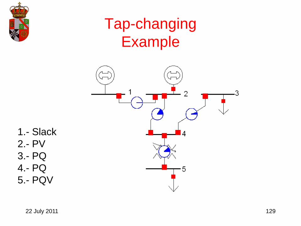
Tap-changing
Example
1.- Slack
2.- PV
3.- PQ
4.- PQ
5.- PQV

22 July 2011 130
Tap-changing
Example
Data:
Line impedances: 0.001+j0.05 p.u.
Shunt admitances: j0.05 p.u. (2 per line).
Transformer: 0.9<t<1.1, steps of 0.005; Zcc=j0.1.

22 July 2011 131
Tap-changing
Example
Bus Voltage (pu). Power
1 1.00 Slack
2 1.00 Pg=150MW
3 -- Pc=50MW, Qc=10MVAr
4 -- Pc=0MW, Qc=0MVAr
5 1.00 Pc=100MW,Qc=50MVAr

22 July 2011 132
Tap-changing
Example
1 32 4
5
shuntYshuntYshuntYshuntY
shuntY shuntY
líneaY líneaY líneaY
tYcc
2cct
t1Y
t
1tYcc
22 July 2011 133
Tap-changing
Example
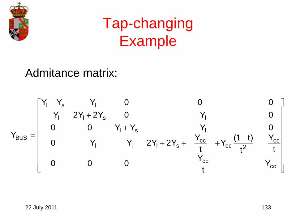
Admitance matrix:
cccc
cc2cc
ccslll
lsl
lsll
lsl
BUS
Yt
Y000
t
Y
t
)t1(Y
t
YY2Y2YY0
0YYY00
0Y0Y2Y2Y
000YYY
Y

22 July 2011 134
Tap-changing
Example
10j10j000
10j884.49j7997.0992.19j3998.0992.19j3998.00
0992.19j3998.0942.19j3998.000
0992.19j3998.00884.39j7997.0992.19j3998.0
000992.19j3998.0942.19j3998.0
Ybus
Variable initial values:
;1t
;1VV
;0
43
5432
22 July 2011 135
Tap-changing
Example
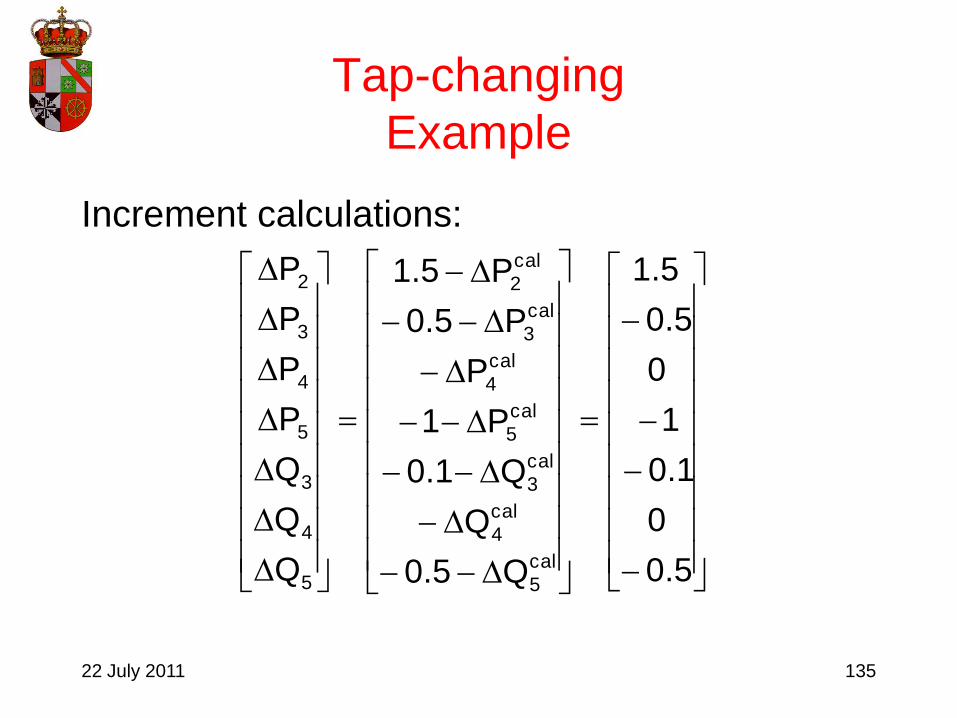
Increment calculations:
5.0
0
1.0
1
0
5.0
5.1
Q5.0
Q
Q1.0
P1
P
P5.0
P5.1
Q
Q
Q
P
P
P
P
cal
5
cal
4
cal
3
cal
5
cal
4
cal
3
cal
2
5
4
3
5
4
3
2

22 July 2011 136
Tap-changing
Example
101000000
10754.49992.1907997.03998.03998.0
0992.19892.1903998.03998.00
000101000
07997.03998.010984.49992.19992.19
03998.03998.00992.19992.190
03998.000992.190984.39
J
Jacobian

22 July 2011 137
Tap-changing
Example
First iteration:
918.0t;
1744.0
0744.0
0993.0
0
0
;
1
968.0
9623.0
1
1
V
082.0
032.0
0377.0
1744.0
0744.0
0993.0
0
t
t
V
V
V
V
4
4
3
3
5
4
3
2

22 July 2011 138
Tap-changing
Example
Admitance matrix:
10j893.10j000
8933.10j750.51j7997.099.19j399.0992.19j3998.00
0992.19j3998.094.19j3998.000
0992.19j3998.00884.39j7997.0992.19j3998.0
00099.19j3998.0942.19j3998.0
Ybus

22 July 2011 139
Tap-changing
Example
Power computation:
492.0
1027.0
1407.0
5647.0
05.0
Q
Q
Q
Q
Q
0527.1
069.0
4657.0
4521.1
0
P
P
P
P
P
5
4
3
2
1
5
4
3
2
1

22 July 2011 140
Tap-changing
Example
Power increments:
008.0
1027.0
0407.0
0527.0
069.0
0343.0
0479.0
492.05.0
1027.0
1407.01.0
0527.11
069.0
4657.05.0
4521.15.1
Q
Q
Q
P
P
P
P
5
4
3
5
4
3
2

22 July 2011 141
Tap-changing
Example
Jacobian matrix:
492.10492.1000527.10527.100
746.115934.486261.180527.16803.00912.08242.1
06075.183261.1808359.08359.00
0527.10527.10492.10492.1000
0527.18183.00912.0492.103879.486261.182698.19
08359.00954.006075.186075.180
00523.1003273.1909193.39
J

22 July 2011 142
Tap-changing
Example
Second iteration
9144.0t;
1723.0
0744.0
1043.0
0002.0
0
;
1
9644.0
9607.0
1
1
V
0039.0
0037.0
0016.0
0021.0
003.0
005.0
0002.0
t
t
V
V
V
V
4
4
3
3
5
4
3
2

22 July 2011 143
Tap-changing
Example
Admitance matrix:
10j9365.10j000
9365.10j8447.51j7997.0992.19j3998.0992.19j3998.00
0992.19j3998.0942.19j3998.000
0992.19j3998.00884.39j7997.0992.19j3998.0
000992.19j3998.0942.19j3998.0
Ybus

22 July 2011 144
Tap-changing
Example
Power calculations:
4999.0
0006.0
1000.0
6391.0
0501.0
Q
Q
Q
Q
Q
0000.1
000.0
4998.0
4998.1
0031.0
P
P
P
P
P
5
4
3
2
1
5
4
3
2
1

22 July 2011 145
Tap-changing
Example
Power increments:
3
5
4
3
5
4
3
2
10
1218.0
6375.0
0339.0
0258.0
0057.0
1969.0
2065.0
4999.05.0
0006.0
1000.01.0
0000.11
000.0
4998.05.0
4998.15.1
Q
Q
Q
P
P
P
P

22 July 2011 146
Tap-changing
Example
Tap to the closest feasible value:
Admitance matrix:
915.0t9144.0t
10929.10000
929.108282.517997.0992.193998.0992.193998.00
0992.193998.0942.193998.000
0992.193998.00884.397997.0992.193998.0
000992.193998.0942.193998.0
jj
jjjj
jj
jjj
jj
Ybus

22 July 2011 147
Tap-changing
Example
Power calculation:
4926.0
0075.0
1000.0
6391.0
0501.0
Q
Q
Q
Q
Q
9993.0
0007.0
4998.0
4998.1
0031.0
P
P
P
P
P
5
4
3
2
1
5
4
3
2
1

22 July 2011 148
Tap-changing
Example
Power increment calculations:
5
5
4
4
3
3
5
4
3
2
5
4
3
5
4
3
2
V
V
V
V
V
V;
0074.0
0075.0
0000.0
0007.0
0007.0
0002.0
0002.0
4926.05.0
0075.0
1000.01.0
9993.01
0007.0
4998.05.0
4998.15.1
Q
Q
Q
P
P
P
P

22 July 2011 149
Tap-changing
Example
Jacobian:
5074.94926.1009993.09993.000
4926.101983.485271.189993.07445.01282.0872.1
05072.183071.1808689.08689.00
9993.09993.004926.104926.1000
9993.07431.01282.04926.102132.485271.181935.19
08689.01307.005072.185072.180
0103.100253.1902449.39
J

22 July 2011 150
Tap-changing
Example
Final values
1725.0
0744.0
1043.0
0002.0
0
;
9991.0
9644.0
9607.0
1
1
V10
8522.0
0558.0
0552.0
1699.0
0152.0
0289.0
0007.0
V
V
V
V
V
V 3
5
5
4
4
3
3
5
4
3
2

22 July 2011 151
Tap-changing
Example
Final power values:
5000.0
000.0
1000.0
6402.0
0501.0
Q
Q
Q
Q
Q
0000.1
0000.0
5000.0
5000.1
0031.0
P
P
P
P
P
5
4
3
2
1
5
4
3
2
1

22 July 2011 152
Power World

22 July 2011 153
5. Fast decoupled AC load flow

22 July 2011 154
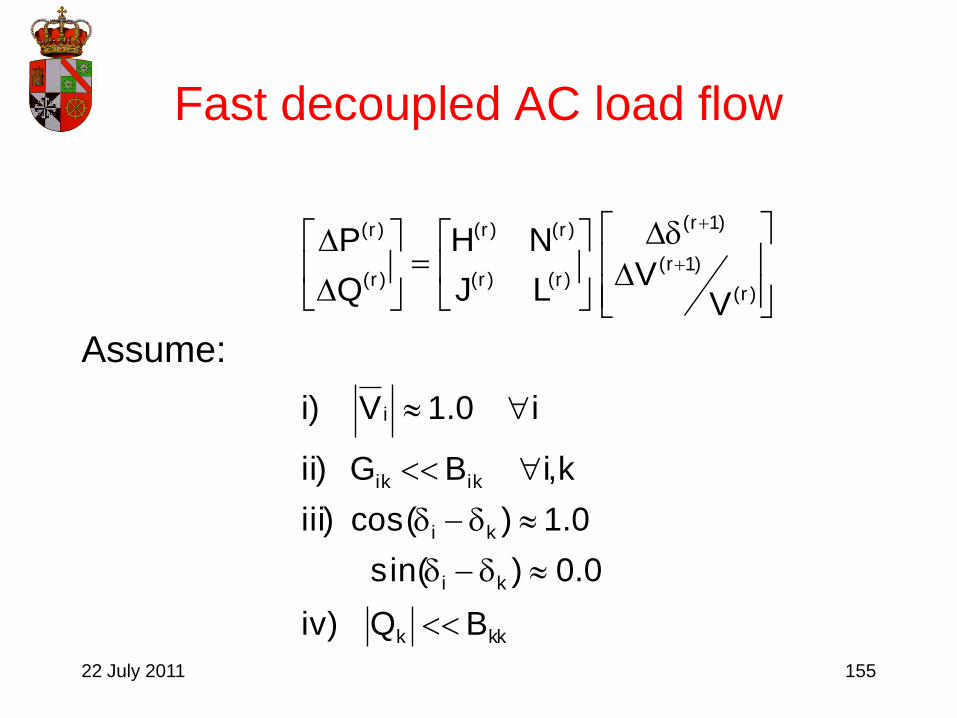
Fast decoupled AC load flow
Two simplifications:
– Do not build Jacobian at each iteration (small error
introduced, then, the procedure needs more
iterations to reach the solution)
– Decoupling between P-δ and Q-V (not
recommended in system highly loaded and/or with
low voltage levels)
22 July 2011 155
Fast decoupled AC load flow
Assume:
kkk
ki
ki
ikik
i
)r(
)1r(
)1r(
)r()r(
)r()r(
)r(
)r(
BQ)iv
0.0)sin(
0.1)cos()iii
k,iBG)ii
i0.1V)i
VV
LJ
NH
Q
P

22 July 2011 156
Fast decoupled AC load flow
We have:
BUS
iiii
ikik21
21
YofElementsBB
~
BB~
B~
,B~
0J,0N,B~
L,B~
H

22 July 2011 157
Fast decoupled AC load flow
)r(1
2)1r(
)r(1
1)1r(
)1r(2
)r(
)1r(1
)r(
)1r(
)1r(
2
1
)r(
)r(
QB~
V
PB~
)2(VB~
Q
)1(B~
P
VB~
0
0B~
Q
P
Use Newton-Raphson Iteration

22 July 2011 158
Fast decoupled load flow. Flow diagram DATA INPUT
Solve (1) and update angles
Solve (2) and update V
OUTPUT RESULTS
YES YES
YES YES
NO
NO
NO
Reactive power
coverged ?
Reactive power
coverged
?
Real power
coverged
?
Real power
coverged ?
Calculate Delta P
NO
NO
Calculate Delta Q

22 July 2011 159
Fast decoupled load flow. Matlab Code
function [V_modulo, V_fase, P, Q, N_iter, T_calculo, Error_p] = desacoplado(V_modulo_ini, V_fase_ini, P_ini, Q_ini, Y, npv)
%
% [V_modulo, V_fase, P, Q, N_iter, T_calculo, Error_p] = desacoplado(V_modulo_ini, V_fase_ini, P_ini, Q_ini, Y, npv)
%
% Obtencion de indices de nodos: 1 -> SLACK;
% 2,...,M -> PV;
% M+1,...,N -> PQ
n = length(V_modulo_ini);
m = npv + 1;
% Parametros del Metodo
Tol = 0.0001; % Tolerancia del metodo (Perdida de potencia).
Error_p = 1; % Error inicial (A un valor mayor que Tol).
N_iter = 0; % Numero de iteraciones.
% Valores iniciales
V_modulo= V_modulo_ini';
V_fase = V_fase_ini';
V = V_modulo.*exp(j*V_fase); % Expresion compleja de la tension
P = P_ini';
Q = Q_ini';
DS_DA = diag(V)*conj(Y*j*diag(V)) + diag(conj(Y*V))*j*diag(V);
DS_DV = diag(V)*conj(Y*diag(V./V_modulo)) + diag(conj(Y*V))*diag(V./V_modulo);
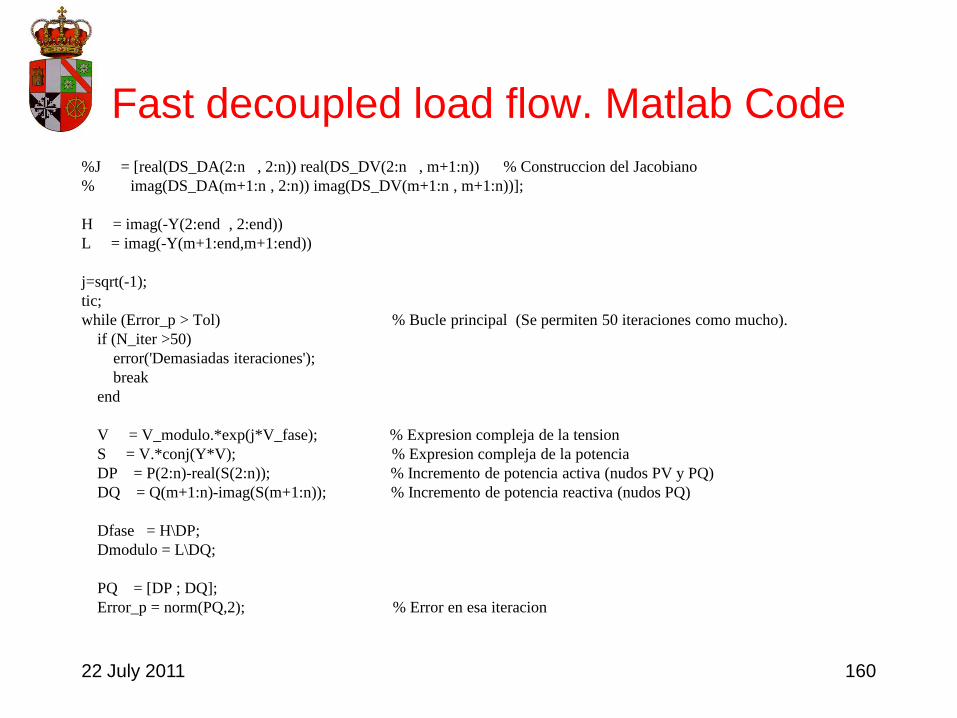
22 July 2011 160
Fast decoupled load flow. Matlab Code
%J = [real(DS_DA(2:n , 2:n)) real(DS_DV(2:n , m+1:n)) % Construccion del Jacobiano
% imag(DS_DA(m+1:n , 2:n)) imag(DS_DV(m+1:n , m+1:n))];
H = imag(-Y(2:end , 2:end))
L = imag(-Y(m+1:end,m+1:end))
j=sqrt(-1);
tic;
while (Error_p > Tol) % Bucle principal (Se permiten 50 iteraciones como mucho).
if (N_iter >50)
error('Demasiadas iteraciones');
break
end
V = V_modulo.*exp(j*V_fase); % Expresion compleja de la tension
S = V.*conj(Y*V); % Expresion compleja de la potencia
DP = P(2:n)-real(S(2:n)); % Incremento de potencia activa (nudos PV y PQ)
DQ = Q(m+1:n)-imag(S(m+1:n)); % Incremento de potencia reactiva (nudos PQ)
Dfase = H\DP;
Dmodulo = L\DQ;
PQ = [DP ; DQ];
Error_p = norm(PQ,2); % Error en esa iteracion

22 July 2011 161
Fast decoupled load flow. Matlab Code
V_fase (2:n) = V_fase(2:n) + Dfase; % Actualizamos la fase de las tensiones (nudos PV y PQ)
V_modulo (m+1:n)= V_modulo(m+1:n) + Dmodulo; % Actualizamos el modulo de las tensiones (nudos PQ)
N_iter = N_iter + 1; % Incremento el numero de iteraciones
% disp('Pulse una tecla para continuar')
% pause
end
P=real(S); % Calculo de la potencia activa
Q=imag(S); % Calculo de la potencia reactiva
V_fase=V_fase*180/pi; % Paso de Radianes a grados
T_calculo=toc;
% **** ENTRADAS ****
%
% V_modulo_ini = Modulo de la tension para comenzar a iterar (conocidos en SLACK y PV).
% V_fase_ini = Fase de la tension para comenzar a iterar (conocido en SLACK).
% P_ini = Potencia activa en los nodos (conocido en PV y PQ).
% Q_ini = Potencia reactica en los nodos (conocido en PQ).
% Y = Matriz de admitancias nodales.

22 July 2011 162
Fast decoupled load flow. Matlab Code
% **** SALIDAS ****
%
% V_modulo = Modulo de la tension en todos los nodos.
% V_fase = Fase de la tension en todos los nodos.
% P = Potencia activa en todos los nodos.
% Q = Potencia reactiva en todos los nodos.
% N_iter = Numero de iteraciones.
% T_calculo = Tiempo de calculo.
% Error_p = Error.
%
%
% **** OBSERVACIONES ****
%
% Los nodos deben estar ordenador asi:
%
% * 1 : SLACK.
% * 2...m : PV.
% * m+1...n : PQ.
%
%
% **** FECHA Y AUTOR ****
%
% Laura Laguna - Nobiembre de 2005

22 July 2011 163
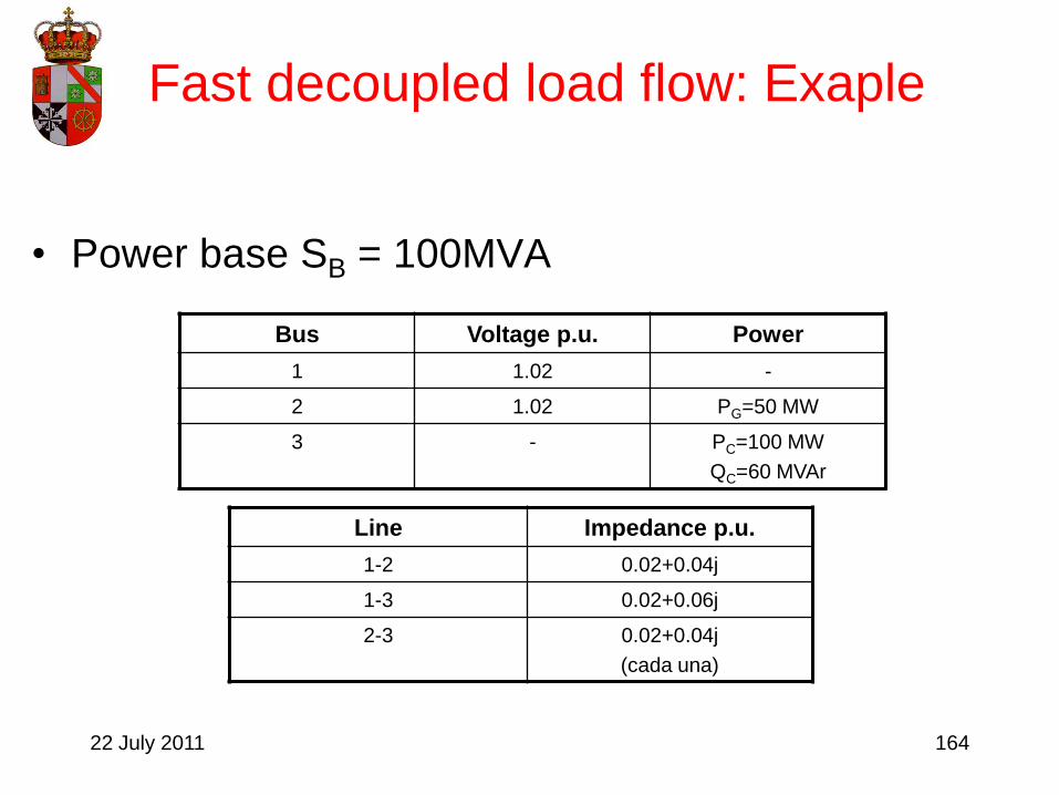
Fast decoupled load flow: Exaple
• Tolerance 0.1 MVA.
ONE TWO
THREE
22 July 2011 164
Fast decoupled load flow: Exaple
• Power base SB = 100MVA
Bus Voltage p.u. Power
1 1.02 -
2 1.02 PG=50 MW
3 - PC=100 MW
QC=60 MVAr
Line Impedance p.u.
1-2 0.02+0.04j
1-3 0.02+0.06j
2-3 0.02+0.04j
(cada una)

22 July 2011 165
Fast decoupled load flow: Exaple
• Admitance matrix
j5525j4020j155
j4020j6030j2010
j155j2010j3515
busY

22 July 2011 166
Fast decoupled load flow: Exaple
• Data and unknown:
Bus Type Data Unknown
1Slack and
reference
V1 = 1.02
δ1=0.0P1, Q1
2 PVP2 =0.5
V2 = 1.02δ2, Q2
3 PQP3 = -1.0
Q3 = -0.6δ3, V3
• Inicialization:
δ2 = δ3 = 0.0 ; V3 = 1.02 p.u.

22 July 2011 167
• Flow diagram
Fast decoupled load flow: Exaple
Vi(0) , δi
(0), Piesp, Qi
esp
Compute: Pical, Qi
cal
Compute: Delta Q
Convergence P?
Compute: Delta P
Solve subproblem 1 and update angles
Final results
Convergence Q?
Solve subproblem 2 and update voltages
Convergence P?Convergence Q?
NO
NO
Yes
Yes
Yes
Yes
NO
NO

22 July 2011 168
Fast decoupled load flow: Exaple
Compute
Calculate P and Q:
No convergence
55L;5540
4060H
6.0
1
5.0
Q6.0
P1
P5.0
Q
P
P
10·2475.7
0
10·3624.0
Q
P
P
cal
3
cal
3
cal
2
3
3
2
15
14
cal
3
cal
3
cal
2

22 July 2011 169
Fast decoupled load flow: Exaple
• First iteration:
0.0109-
1.3481-
0.4213-
VV
3
3
3
2
1.3481-
0.4213-
0
;
0091.1
0200.1
0200.1
V

22 July 2011 170
Fast decoupled load flow: Exaple
Residuals:
Error = 0.5976 → no convergence
4583.0
3003.0
2385.0
Q6.0
P1
P5.0
Q
P
P
1417.0
3003.1
7385.0
Q
P
P
cal
3
cal
3
cal
2
3
3
2
cal
3
cal
3
cal
2

22 July 2011 171
Fast decoupled load flow: Exaple
• System state (second iteration)
0.0083-
0.2857
0.0372-
VV
3
3
3
2
1.0264-
0.4585-
0
;
0008.1
0200.1
0200.1
V

22 July 2011 172
Fast decoupled load flow: Exaple
•Residuals:
•Error = 0.2885 → no convergence
1444.0
1936.0
1578.0
Q6.0
P1
P5.0
Q
P
P
7444.0
1936.1
6578.0
Q
P
P
cal
3
cal
3
cal
2
3
3
2
cal
3
cal
3
cal
2

22 July 2011 173
Fast decoupled load flow: Exaple
• System state (third iteration):
• The process continues.
0.0026
0.1788
0.0315-
VV
3
3
3
2
0.8836-
0.4900-
0
;
0034.1
0200.1
0200.1
V

22 July 2011 174
Fast decoupled load flow: Exaple
•After 9 iterations:
•Error = 0.0012 → convergence attained
3
3
3
cal
3
cal
3
cal
2
3
3
2
cal
3
cal
3
cal
2
10·3346.8
10·7006.0
10·5954.0
Q6.0
P1
P5.0
Q
P
P
5992.0
0007.1
5006.0
Q
P
P

22 July 2011 175
Fast decoupled load flow: Exaple
• System state at iteration 10:
5-
3-
3-
3
3
3
2
1.5154·10-
0.6141·10
0.1592·10-
VV
0.9614-
0.4710-
0
;
0043.1
0200.1
0200.1
V

22 July 2011 176
Fast decoupled load flow: Exaple
•Residuals:
•Error = 5.6285·10-4 → convergence attained
4
3
3
cal
3
cal
3
cal
2
3
3
2
cal
3
cal
3
cal
2
10·3349.3
10·3516.0
10·2863.0
Q6.0
P1
P5.0
Q
P
P
6003.0
0004.1
5003.0
Q
P
P
22 July 2011 177
Fast decoupled load flow: Exaple
• State at iteration 11:
6-
3-
3-
3
3
3
2
6.0634·10
0.3251·10
0.0567·10-
VV
0.9611-
0.4711-
0
;
0043.1
0200.1
0200.1
V
6003.0
5515.0
0711.0
Q
0004.1
5003.0
5098.0
P

22 July 2011 178
Fast decoupled load flow: Exapleconvergence
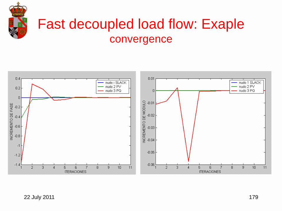
22 July 2011 179
Fast decoupled load flow: Exapleconvergence

22 July 2011 180
Fast decoupled load flow: Exapleconvergence

22 July 2011 181
Fast decoupled load flow: Exapleconvergence

22 July 2011 182
6. Variable limits
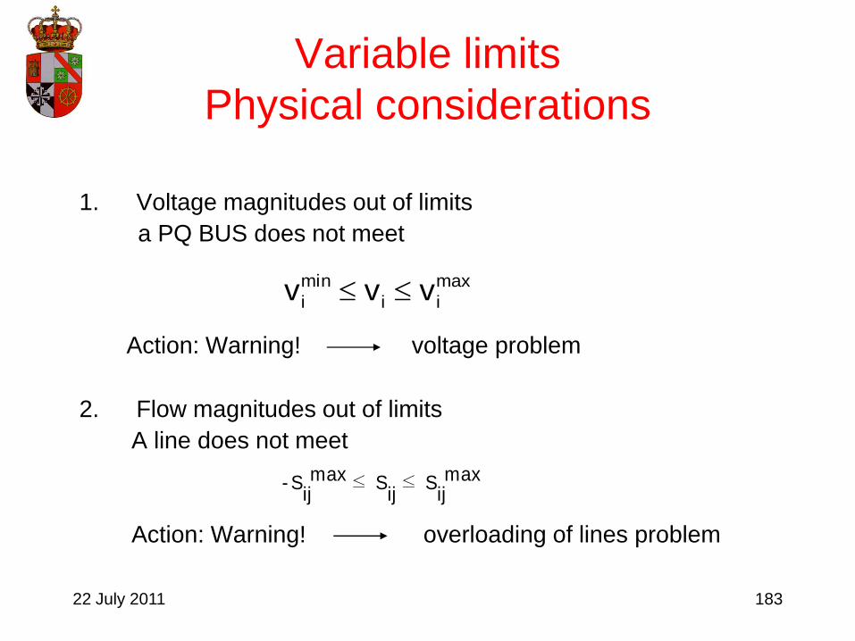
22 July 2011 183
Variable limits
Physical considerations
1. Voltage magnitudes out of limits
a PQ BUS does not meet
Action: Warning! voltage problem
2. Flow magnitudes out of limits
A line does not meet
Action: Warning! overloading of lines problem
maxij
S ij
S maxij
S- ≤≤
max
ii
min
i vvv

22 July 2011 184
Variable limits
Physical Considerations
3. Reactive Power out of limits
A PV BUS does not meet
Action: Wrong Formulation!
Specified voltage cannot be attained
Formulate the problem properly
maxi i
mini Q Q Q

22 July 2011 185
Q hits
limit?
yes
QG>Qmax?Yes Change to
P-Q
Q=Qmax
QG<Qmin?
Yes
No
Change to
P-Q
Q=Qmin
Stay as
P-V
No
no
Q=Qmax ?
yes
V >Vdato?Change to P-V
V=Vdato
Stay as
P-Q
no
Yes
V <Vdato?Change to P-V
V=Vdato
NoStay as
P-Q
Variable limits
Computational Considerations
Changing PV to PQ
Yes
No

22 July 2011 186
7. DC load flow

22 July 2011 187
DC load flow
• Approximate solution.
• Two simplifications:
– In network model: do not consider series
resistences and shunt admittances
– Assume Vi=1 at all buses

22 July 2011 188
DC load flow
Approximate analytical solution
Assume
0.1 cos)iii
sin)ii
i0.1 V)i
ijcos
ijX
jV
iV
ijX
2
iV
ijQ
ijsin
ijX
jV
iV
ijP
ij
ijij
i
≈
≈
∀≈
-

22 July 2011 189
DC load flow
Approximate analytical solution
where
ij'ij
n
ij1j
ij'ii
n
ij1j
jiji
n
ij1j
n
ij1j
ijiji
jijiijijijij
ijij
BB
BB
´BP
BBPP
BBBX
P

22 July 2011 190
DC load flow
Continuation
VBQ
VBVBQQ
VBVB)VV(BX
VVQ
'
j
n
ij1j
iji
n
ij1j
ij
n
ij1j
iji
jijiijjiij
ij
ji
ij

22 July 2011 191
DC load flow
Continuation
Solution
ij
ij
ij
'
ij
n
ij1j
ij
'
ii'
n
1m
n
2
n
1
n
1
'
'
X
1B;
BB
BB
B
Q
Q
Q;
P
P
P;
V
V
V;
BusesPQVBQ
BusesPV&PQBP

22 July 2011 192
DC Power flow: example

22 July 2011 193
DC Power flow: example
ONE TWO
THREE

22 July 2011 194
Data
Bus Voltage p.u. Power
0 1.02 -
1 1.02 PG=50MW
2 - PC=100MW, QC=60MVAr
Line Impedance p.u.
0-1 0.02+0.04j
0-2 0.02+0.06j
1-2 0.02+0.04j (both)
DC Power flow: example

22 July 2011 195
DC Power flow: example
2
1
0
2
1
0
V
02.1
02.1
67.665067.16
507525
67.162567.41
6.0
Q
Q
0
67.665067.16
507525
67.162567.41
0.1
5.0
P
67.665067.16
507525
67.162567.41
B

22 July 2011 196
DC Power flow: example
2
1
0 0
67.665067.16
507525
67.162567.41
0.1
5.0
P

22 July 2011 197
Po= -25δ1 - 16.67δ2
0.5= +75δ1 - 50δ2
-1.0= -50δ1 + 66.67δ2
Q0= 41.67*1.02 - 25*1.02 - 16.67V2
Q1= -25*1.02 + 75*1.02 - 50V2
-0.6= -16.67*1.02 - 50*1.02 + 66.67V2
DC Power flow: example

22 July 2011 198
Solution:
P0 0.5p.u.=50MW
Q0 0.15p.u.=15MVAr
Q1 0.45p.u.=45MVAr
δ1 -1.1459º
δ2 -0.3819º
V2 1.011p.u.
DC Power flow: example

22 July 2011 199
PowerWorld comparison:
Var DC PowerWorld DC PowerWorld G-S
P0 0.50p.u. 0.50p.u. 0.509p.u.
Q0 0.15p.u. 0.00p.u. 0.07p.u.
Q1 0.45p.u. 0.00p.u. 0.55p.u.
δ1 -0.3819 -0.3820 -0.47
δ2 -1.1459 -1.1459 -0.96
V2 1.0056p.u. 1.0000p.u. 1.0043p.u.
DC Power flow: example

22 July 2011 200
DC Power flow: example
UNO
DOS
CERO
0,00 MW 0,00 Mvar
50,00 MW 0,00 Mvar
TRES
100,00 MW
60,00 Mvar

22 July 2011 201
Data.
Bus Voltage p.u. Power
0 1.02 -
1 1.02 PG=50MW
2 - PC=0MW, QC=0MVAr
3 - PC=100MW, QC=60MVAr
Line Impedance p.u.
0-1 0.02+0.04j
0-2 0.02+0.06j
1-2 0.02+0.04 (both)
2-3 0.1j
DC Power flow: example

22 July 2011 202
DC Power flow: example
3
2
1
0
3
2
1
0
V
V
02.1
02.1
101000
1067.765067.16
0507525
067.162567.41
6.0
0.0
Q
Q
0
101000
1067.765067.16
0507525
067.162567.41
0.1
0.0
5.0
P
101000
1067.765067.16
0507525
067.162567.41
B
22 July 2011 203
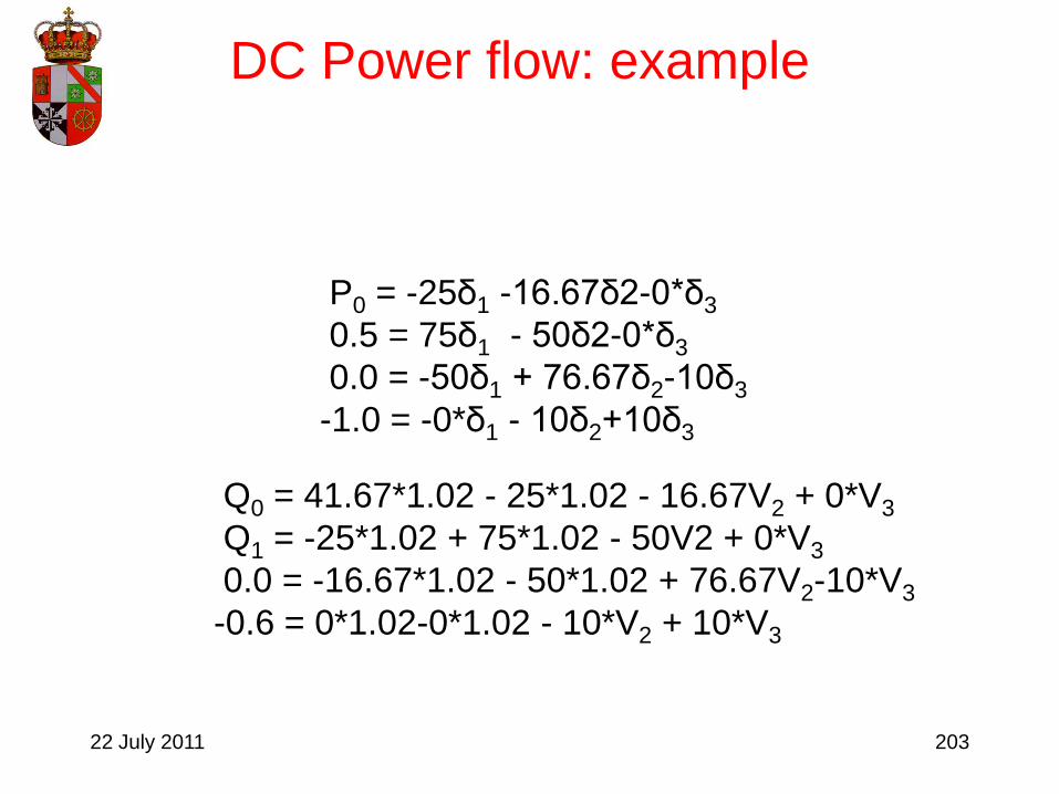
P0 = -25δ1 -16.67δ2-0*δ3
0.5 = 75δ1 - 50δ2-0*δ3
0.0 = -50δ1 + 76.67δ2-10δ3
-1.0 = -0*δ1 - 10δ2+10δ3
Q0 = 41.67*1.02 - 25*1.02 - 16.67V2 + 0*V3
Q1 = -25*1.02 + 75*1.02 - 50V2 + 0*V3
0.0 = -16.67*1.02 - 50*1.02 + 76.67V2-10*V3
-0.6 = 0*1.02-0*1.02 - 10*V2 + 10*V3
DC Power flow: example

22 July 2011 204
PowerWorld comparison:
Var DC PowerWorld G-S PowerWorld DC
P0 0.50p.u. 0.51p.u. 0.50p.u.
Q0 0.00p.u. 0.11p.u. 0.00p.u.
Q1 0.00p.u. 0.67p.u. 0.00p.u.
δ1 -0.3819º -0.48º -0.382º
δ2 -1.1459º -0.91º -1.1459º
δ3 -6.8755º -7.05º -6.8755º
V2 1.011p.u. 1.002p.u. 1.000p.u.
V3 0.951p.u. 0.932p.u. 1.000p.u.
DC Power flow: example

22 July 2011 205
8. Comparison of load flow
solution methods

22 July 2011 206
Comparison of load flow methods
1. Gauss-Seidel (G-S)
Simple technique
Iteration time increases linearly with the
number of buses. Lower iteration time than N-
R. Seven times faster in large systems
Linear rate of convergence. Many iterations
required for getting close to the solution
Number of iteration increases with the
number of buses

22 July 2011 207
Comparison of load flow methods
(Continuation)
2. Newton-Raphson (N-R)
Widely used
Iteration-time increases linearly with the number of buses
Quadratic rate of convergency. A few iterations for getting close to the solution
Number of iterations independent of the number of buses of the system
The Jacobian is a very sparse matrix
Method non-sensitive to slack bus choice and the presence of series capacitors
Sensitive to initial solution

22 July 2011 208
Comparison of load flow methods
(Continuation)
3. AC decoupled
has to be computed and factorized only once
It requires more iterations than Newton-Raphson method
Iteration time is 5 times lower than Newton-Raphson´s iteration time
Useful for analyzing topology changes because can be easily modified
Used in planning and contigency analyses
B~
B~

22 July 2011 209
Comparison of load flow methods
(Continuation)
4. DC Decoupled
Analytical, approximate and non-iterative method
Good approximation for , not that good
approximation for
Used in reliability analyses
Used in optimal pricing calculations
Good for getting an initial point
V


![20121105 no tempest in my teapot [dlf forum denver]](https://static.documents.pub/doc/80x56/554bd55fb4c9058f6c8b5024/20121105-no-tempest-in-my-teapot-dlf-forum-denver.jpg)


