The London School of Economics and Political Science Essays on the Relation between Accounting and Employment, Risk and Valuation Daphne Hart A thesis submitted to the Department of Accounting of the London School of Economics and Political Science for the degree of Doctor of Philosophy January 2019
Transcript
0
The London School of Economics and
Political Science
Essays on the Relation between Accounting
and Employment, Risk and Valuation
Daphne Hart
A thesis submitted to the Department of Accounting of the London
School of Economics and Political Science for the degree of Doctor of
Philosophy
January 2019
1
Declaration
I certify that the thesis I have presented for examination for the MPhil/PhD degree of
the London School of Economics and Political Science is solely my own work other than
where I have clearly indicated that it is the work of others (in which case the extent of any
work carried out jointly by me and any other person is clearly identified in it).
The copyright of this thesis rests with the author. Quotation from it is permitted,
provided that full acknowledgement is made. This thesis may not be reproduced without my
prior written consent.
I warrant that this authorization does not, to the best of my belief, infringe the rights
of any third party.
I confirm that Chapter 2 is jointly co-authored with Brian Burnett and Paige Patrick.
I also confirm that Chapter 3 is jointly co-authored with Bjorn Jorgensen.
I declare that my thesis consists of 46,381 words.
2
Acknowledgments
I have been blessed with two exceptional supervisors. No words could fully express
my appreciation and respect for my first supervisor, Bjorn Jorgensen. Thank you for your
support, guidance and faith. Thank you for giving me space to ask questions and make
mistakes. Above all, thank you for teaching me to always keep trying and never give up. These
lessons and our long conversations will forever remain with me.
To my second supervisor, Vasiliki Athanasakou, I am deeply indebted for your
coaching and care. Thank you for being an endless source of inspiration and encouragement,
for always having an open door and an open heart for me. I am grateful for your advice and
for all the times you asked the difficult questions. You helped me grow into myself as an
academic and a person.
I have been privileged to be part of the Department of Accounting for the last four
years, and I am thankful to my friends and colleagues at the London School of Economics. I
am honored to have shared this unique experience with Brett Considine, Nadine de Gannes
and Rani Suleman – thank you for the long coffee chats, for being a sounding board and most
of all, thank you for being such good friends.
Completing this dissertation is almost the last stage of my doctoral journey. I shared
this journey with many wonderful people, whose love and support carried me through. To my
mentors, Asher Tishler and Iris Canor, thank you for your encouragement and for your
guidance over the years. I appreciate our many long discussions about life and academia.
Thank you for sharing your experience with me.
My family has been the driving force behind me. The long days that turned into long
nights were fueled by their love. I knew I was never alone in this - Reuven, Michal, Udi, Itamar
and Galit Pinchas, I could not have done this without you. Thank you for believing in me, for
pushing forward with me and for standing by me. I am thankful to Baias Shila for looking out
for me, I cherish your short yet heart-warming phone calls. Emanuel and Mia Hart, thank you
3
for giving me courage and good advice in critical moments. I am grateful to Galia Finkelstein
for her wisdom and patience and to Irit Meyer for making London feel like home.
To my sister, Miri, who always helps me to make sense of this world and can always
make sense of me. You planted the seed of curiosity in my mind and taught me how to carve
my own path. Thank you for your understanding and love, for making everything feel possible.
My partner and love, Gil Pinchas, who has been with me through every step of the
journey. His faith in me allowed me to dream and his reassurance lifted me over all barriers
and hardship. I could not have hoped for a better partner and friend to share this journey with.
Thank you for being so gracious, shielding, supportive and empowering.
To my parents, Rachel and Ovadia, this thesis is inspired by your experiences. Thank
you for all your hard work over the years, for providing me with every opportunity imaginable.
Thank you for respecting my choices even when the causes were not clear to you (or me). You
opened the world to me, thank you for helping me feel at home no matter where I was. Your
love, determination and generosity travels with me. This dissertation is dedicated to you.
4
Abstract
The thesis is a collection of three separate papers on accounting consequences.
Specifically, the papers examine the relation between accounting and employment, risk and
valuation.
The first chapter (solo-authored) documents that approximately 20% of large US
public firms choose to disclose employment information quarterly, at a higher frequency than
mandated by the US Securities and Exchange Commission (SEC). I use these voluntary
disclosures to examine whether managers modify their firms’ workforces to manage earnings.
Using firm-level analysis, I find that managers alter their firms’ workforce in the short-run to
meet financial reporting benchmarks. I separately investigate the decision to voluntary
disclose employment information more frequently than mandated by the SEC. I show that
providing quarterly employment disclosures is associated with managerial myopic behavior.
Overall, in the first chapter I present evidence that more frequent disclosures of workforce
information provide valuable insights into firm operations and managerial decisions. I
demonstrate that financial measures may govern decisions regarding real resource allocations,
specifically, the firm’s workforce size.
The second chapter (co-authored with Brian Burnett and Paige Patrick) investigates
the effect of adopting more principles-based standards on litigation risk. A common perception
is that principles-based accounting standards, such as International Financial Reporting
Standards (IFRS), allow for more managerial discretion over financial reporting. This suggests
that adopting principles-based standards may alter the litigation risk exposure of companies
and their directors and officers. We study changes in litigation risk in Canada following IFRS
adoption in 2011. Canada switched its reporting standards from Canadian Generally Accepted
Accounting Principles (GAAP) to IFRS, which is considered more principles-based. We
examine the effect of IFRS adoption on litigation risk using two established proxies for
litigation risk: Directors’ and Officers’ (D&O) liability insurance, which Canadian firms are
mandated to disclose, and excess cash holdings. We document that more principles-based
5
accounting standards reduce litigation risk and provide evidence for a benefit of adopting such
standards, in the form of lower insurance premiums.
The third chapter (co-authored with Bjorn Jorgensen) develops an accounting-based
valuation model for an economy with multiple firms and demonstrates the effect of cross-
holdings on firms’ prices. We illustrate how market values appear distorted when firms have
mutual minority interest equity investments. We discuss possible empirical implications for
valuation of multiple firms and articulate why corporate equity investments may distort firms’
market-to-book ratios. Overall, we show how the accounting treatment for corporate equity
investments may alter prices and provide theoretical predictions regarding the mechanism and
magnitude of these distortions. We also model linear information dynamics in a setting with
multiple firms, allowing for inter-firm information transfers for firms with and without cross-
holdings. Our analysis illustrates how inter-firm accounting information shape prices.
Moreover, we describe possible implications of our model for firms that exhibit variation in
reporting dates or reporting frequency.
6
Contents
Declaration of Authorship 1
Acknowledgements 2
Abstract 4
List of Figures 10
List of Tables 11
1. Voluntary Employment Disclosures and Real Earnings Management 12
1.1 Introduction 12
1.2 Employment and Real Earnings Management 16
1.2.1 Firms’ Employment Policies 16
1.2.2 Real Earnings Management and Employment 18
1.2.3 Voluntary Employment Disclosure and Myopic Behavior 20
1.3 Data and Methodology 23
1.3.1 Employment Data 23
1.3.2 Normal Employment Model 28
1.3.3 Selection of Suspect Firm-quarters 31
1.4 Empirical Analysis 32
1.4.1 Choice Model Estimation 32
1.4.2 Abnormal Employment Estimation 33
1.4.3 Real Earnings Management 34
1.4.4 Subsequent Performance 38
1.5 Voluntary Employment Disclosure and Managerial Behavior 40
1.6 Conclusion 41
1.7 Appendix 43
1.7.1 Variable Descriptions 43
1.8 Figure 45
1.8.1 Changes in Disclosure Policy (Non-Financial Firms) 45
1.9 Tables 46
1.9.1 Descriptive Statistics 46
1.9.2 Number of Firms and Disclosing Firms by Industry Division 47
1.9.3 Descriptive Statistics: Disclosure Choice Model 48
7
1.9.4 Regression Results: Estimation of the Disclosure Choice Model 49
1.9.5 Descriptive Statistics: Disclosing Firms 50
1.9.6 Regression Results: Estimation of the labor model 51
1.9.7 Comparison of Suspect Firm-quarters with the Rest of the Sample 52
1.9.8 Comparison of Suspect Firm-quarters with the Rest of the Sample,
Full Interaction
53
1.9.9 Regression Results: Future Performance 54
1.9.10 Regression Results: Probability of Just Meeting or Beating Earnings
Benchmarks
55
2. IFRS Adoption and Litigation Risk: Evidence from Directors’ and
Officers’ Liability Insurance
56
2.1 Introduction 56
2.2 Directors’ and Officers’ (D&O) Liability Insurance 61
2.3 Hypothesis Development 64
2.4 Research Design 67
2.4.1 The Canadian Setting 67
2.4.2 Canadian Firms Cross-listed in the US 68
2.4.3 Specifications 69
2.4.4 Sample Selection and Data Description 74
2.5 Empirical Results 77
2.5.1 Univariate Results 77
2.5.2 Regression Analyses of D&O Insurance Policy 79
2.5.3 Regression Analyses of Excess Cash 81
2.6 Robustness Tests 82
2.7 Conclusion 84
2.8 Appendix 86
2.8.1 Variable Descriptions 86
2.9 Tables 88
2.9.1 Sample Formation 88
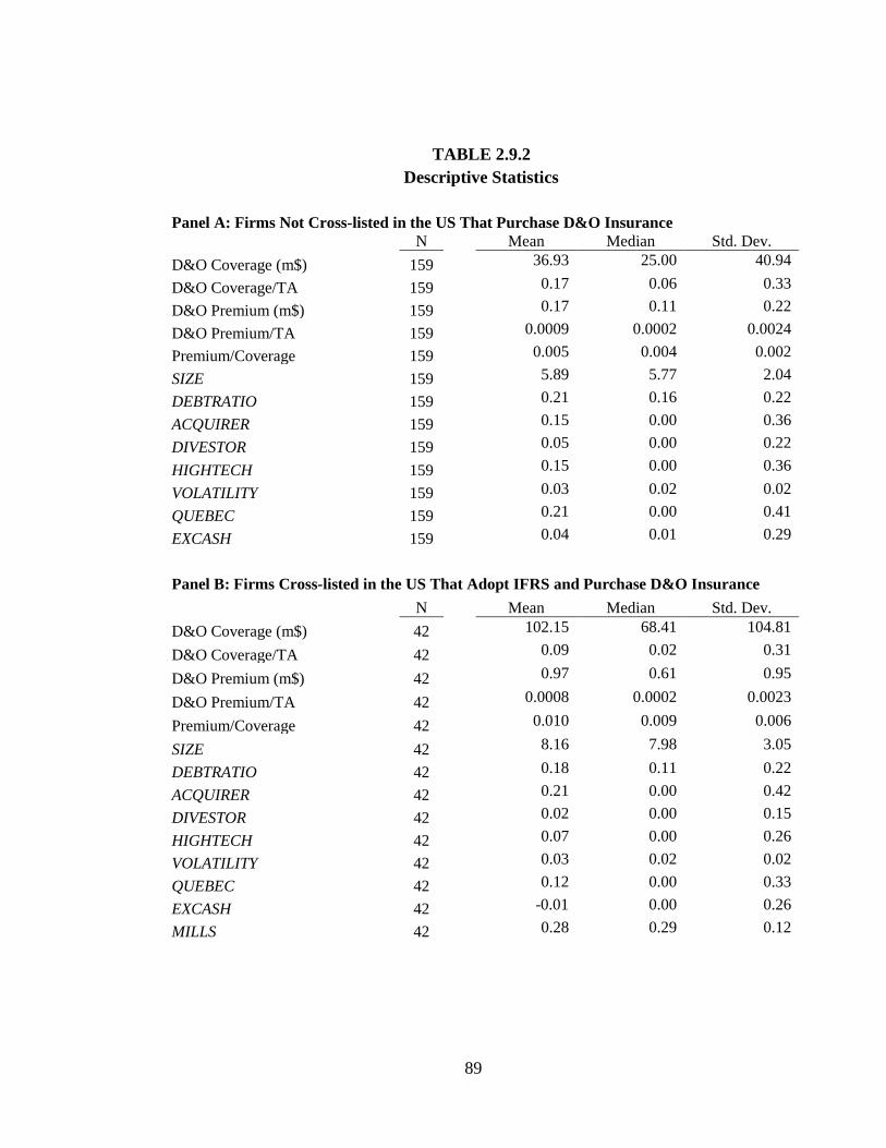
2.9.2 Descriptive Statistics 89
2.9.3 Univariate Tests of Changes in D&O Coverage and Premiums After
IFRS Adoption
91
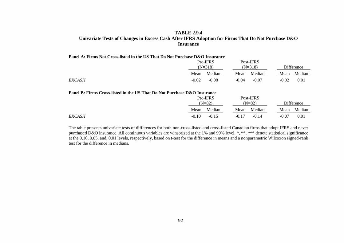
2.9.4 Univariate Tests of Changes in Excess Cash After IFRS Adoption for
Firms That Do Not Purchase D&O Insurance
92
2.9.5 Regression of the Effect of IFRS Adoption on D&O Coverage and
Premiums for Canadian Firms Not Cross-listed in the US
93
8
2.9.6 Regression of the Effect of IFRS Adoption on D&O Coverage and
Premiums for Canadian Firms Cross-listed in the US
94
2.9.7 Regression of the Effect of IFRS Adoption on Excess Cash for
Canadian Firms Not Cross-listed in the US That Do Not Purchase D&O
Insurance
95
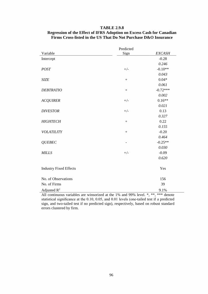
2.9.8 Regression of the Effect of IFRS Adoption on Excess Cash for
Canadian Firms Cross-listed in the US That Do Not Purchase D&O
Insurance
96
2.9.9 Descriptive Statistics for New York State Incorporated Firms 97
2.9.10 Regression of the Effect of IFRS Adoption on Premiums for
Canadian Firms Cross-listed in the US Compared to Firms Incorporated in
New York State
98
3. Accounting-Based Valuation for Multiple Firms: The Case of Cross
Holdings
99
3.1 Introduction 99
3.2. A Valuation Model with Corporate Equity Ownership 105
3.2.1 Formal Model of Cross Holdings 105
3.2.2 Implication for Empirical Research: The Case of Cross Holdings 113
3.2.3 Price and Book Values: The Effect of Cross Holdings on Financial
Ratios
120
3.3. Uncertainty and Linear Information Dynamics 121
3.3.1 Inter-Firm Information Transfers: Multiple Firms 122
3.3.2 Linear Information Dynamics and Firm Valuation: The Case of Two
Firms
125
3.3.3 Linear Information Dynamics and Firm Valuation: Cross Holdings 128
3.4. Conclusion 130
3.5 Appendices 133
3.5.1 Variable Definitions 133
3.5.2 Illustration of Two Firms with Cross Holdings Using the Fair Value
Method
135
3.5.3 Illustration of Two Firms with Cross Holdings Using the Equity
Method
139
3.5.4 Market-to-Book and Return-on-Equity Ratios 142
3.5.5 Linear Information Dynamics 145
3.5.6 Linear Information Dynamics – Empirical Application 155
1.9.2 Number of Firms and Disclosing Firms by Industry Division 47
1.9.3 Descriptive Statistics: Disclosure Choice Model 48
1.9.4 Regression Results: Estimation of the Disclosure Choice Model 49
1.9.5 Descriptive Statistics: Disclosing Firms 50
1.9.6 Regression Results: Estimation of the labor model 51
1.9.7 Comparison of Suspect Firm-quarters with the Rest of the Sample 52
1.9.8 Comparison of Suspect Firm-quarters with the Rest of the Sample, Full
Interaction
53
1.9.9 Regression Results: Future Performance 54
1.9.10 Regression Results: Probability of Just Meeting or Beating Earnings
Benchmarks
55
2.9.1 Sample Formation 88
2.9.2 Descriptive Statistics 89
2.9.3 Univariate Tests of Changes in D&O Coverage and Premiums After IFRS
Adoption
91
2.9.4 Univariate Tests of Changes in Excess Cash After IFRS Adoption for Firms
That Do Not Purchase D&O Insurance
92
2.9.5 Regression of the Effect of IFRS Adoption on D&O Coverage and
Premiums for Canadian Firms Not Cross-listed in the US
93
2.9.6 Regression of the Effect of IFRS Adoption on D&O Coverage and
Premiums for Canadian Firms Cross-listed in the US
94
2.9.7 Regression of the Effect of IFRS Adoption on Excess Cash for Canadian
Firms Not Cross-listed in the US That Do Not Purchase D&O Insurance
95
2.9.8 Regression of the Effect of IFRS Adoption on Excess Cash for Canadian
Firms Cross-listed in the US That Do Not Purchase D&O Insurance
96
2.9.9 Descriptive Statistics for New York State Incorporated Firms 97
2.9.10 Regression of the Effect of IFRS Adoption on Premiums for Canadian
Firms Cross-listed in the US Compared to Firms Incorporated in New York State
98
3.7.1 Two Firms - Fair Value Method 166
3.7.2 Two Firms -Equity Method 167
3.7.3 Market-to-Book Ratios 168
3.7.4 Return on Equity 169
12
Chapter 1
Voluntary Employment Disclosures and Real Earnings
Management
Daphne Hart*
1.1 Introduction
This chapter studies the employment policies of public firms. While the US Securities
and Exchange Commission (SEC) mandates annual disclosures of a public firm’s number of
employees, approximately 20% of large US firms voluntarily disclose employment quarterly.
Using these voluntary quarterly disclosures, I study whether managers modify their firms'
workforce to meet earnings benchmarks and whether the decision to disclose is associated
with myopic managerial behavior.
In the past decade, technological advances fueled rapid growth in service industries,
reducing the share of capital-intensive industries in the economy (Lee and Wolpin 2006).
Many public firms rely on human capital for their operations and state they view their
employees as an important asset. Nonetheless, the information available to investors and other
stakeholders about the way firms manage their workforces is limited.
*I thank Vasiliki Athanasakou, Bjorn Jorgensen, and Wim Van der Stede for their guidance and support.
I also thank Jan Bouwens, Maria Correia, Thomas Gilliam, Katherine Gunny, Ana Simpson and
workshop participants at Bocconi University, Cambridge University, Cass Business School, Hebrew
University, IESE Business School, London School of Economics and Political Science, Oxford
University, Pompeu Fabra University, Tilburg University, University of Illinois at Chicago and
University of Warwick for their comments and suggestions.
13
The SEC requires public firms to disclose their number of employees annually. The
Business and Financial Disclosure required by Regulation S–K includes a narrative
description of a registrant’s business. Under Regulation S-K, firms must disclose their number
of employees in their annual financial statements.1 Firms are not required to disclose any
information about their workforce in their quarterly financial statements. Nonetheless, some
firms choose to provide this information voluntarily, with quarterly frequency.2
Using a hand collected sample of the largest 500 firms listed on NYSE and NASDAQ
from 2006 until 2016 (44 quarters),3 I document that 20.5% of them provided information
about the size of their workforce in interim financial reports. The choice to provide quarterly
employment information appears relatively sticky over time.4,5 I use these voluntary
disclosures in two ways. First, I examine whether managers appear to alter the workforce to
manage earnings. Second, I investigate the relation between providing voluntary employment
information at higher frequencies and managerial short-termism.
A firm’s economic activity can be represented in price terms (costs, wages, and
interest) or in volume (labor and capital). The literature uses labor costs to estimate managers’
asymmetric responses to changes in operations and to detect managerial opportunism
(Dierynck, Landsman, and Renders 2012, Hall 2016). Annual net changes in the number of
employees (net hiring) are also used to proxy for investment in labor. Pinnuck and Lillis (2007)
examine whether reporting negative earnings influences investments in employees and find a
discontinuity in a histogram of net hiring around zero earnings. Jung, Lee, and Weber (2014)
1 17 CFR 229.101 - Description of business, Item 101(c)(1)(xiii).
2 Interestingly, Beatty and Liao (2017) document that around 20% of US multinationals’ 10-K filings
voluntarily disclose domestic and foreign headcount separately. Their analysis suggests that voluntary
geographic headcount disclosure choice with annual frequency, depends on both political pressure and
employee backlash. 3 I limit the sample to the largest 500 firms listed on NYSE and NASDAQ in the sample period that
report under US Generally Accepted Accounting Principles (GAAP). Out of 749 firms for which data
is available, 154 provide information about their workforces in their interim reports and 143 firms have
consecutive disclosures that permit constructing quarterly time series. 4 In each period, a firm may choose to initiate or cease disclosing the number of employees quarterly.
For example, Pfizer Inc. started providing quarterly employment information in the first quarter of 2010
and ceased quarterly disclosures in the third quarter of 2013. 5 During the sample period, disclosing firms voluntarily disclosed their workforce size for 28 quarters
on average.
14
use firms’ net hiring to construct a measure of investment efficiency. I extend prior literature
and proxy for firm’s real activities using quarterly workforce data. Quarterly data enables
observing managerial decisions, as opposed to inferring them from reported expenses (Cohen,
Mashruwala, and Zach 2010). Having more granular data permits studying changes in the flow
of the size of the work force in the short-run and examining whether managers use employment
to manage earnings.6
A manager could alter the workforce to achieve short-term reporting goals. On the
one hand, managers may decrease the workforce by firing or simply not hiring new employees.
This reduces expenses and cash outflows, thus increasing reported earnings. On the other hand,
managers may choose to increase production to report lower cost of goods sold (COGS) under
absorption costing or to channel stuff (Roychowdhury 2006). These latter practices likely
require hiring additional employees in the short-run, particularly in human capital-intensive
industries like services and high-tech. If managers engage in real earnings management
through net hiring, abnormal patterns in employment should mirror the findings of prior
literature (Roychowdhury 2006, Gunny 2010, Zang 2012).
I document that if firms just meet or beat analysts’ forecasts, or report small earnings
growth, they have larger abnormal workforce, while if they report small positive earnings,
they have smaller abnormal workforce. These results are consistent with managers employing
different producing and employment practices to achieve different reporting goals.
Better understanding firms’ employment policies is important as labor market
frictions generate substantial costs for firms, employees, and the economy. Moreover, the
relationship between employers and employees shape labor laws and employment incentives
schemes. Nonetheless, scant empirical research investigates firms’ employment decisions,
6 The annual number of employees disclosed in firms’ annual reports (10-K form), provides information
about the net change in the workforce over the fiscal year but not within the year. Firms may report the
same number of employees in consecutive years, although, during the year, their workforces may
fluctuate substantially. For example, based on Caterpillar Inc.’s annual number of employees, it appears
that the firm’s net hiring in 2012 was 0.2%. Nonetheless the quarterly employment disclosures suggest
that Caterpillar increased its labor force by 1.7% and 4.4% in the first two quarters and decreased it by
2.8% and 2.9% in the last two quarters of 2012.
15
partly because firm-level employment data is scarce.7 The data set I constructed is based on
voluntary disclosure of large pubic firms, which may limit the generalizability of this paper’s
findings.
I separately investigate the decision to provide quarterly employment disclosures, at
a higher frequency than mandated by the SEC. To signal firm quality, managers may choose
to increase transparency by providing employment information in interim reports (Verrecchia
1983, Dye 1985). If earnings management is a purposeful intervention (Schipper 1989) that
could be inferred from abnormal employment levels, then voluntarily quarterly disclosure may
act as a disciplining mechanism. Thus, quarterly disclosures would be associated with fewer
incidences of just meeting earnings benchmarks. Nonetheless, higher disclosure frequency
may also indicate that managers focus on shorter horizons, implying a positive association
between quarterly employment disclosures and incidences of just meeting earnings
benchmarks.
I find that providing quarterly employment disclosures is associated with a higher
likelihood of just meeting or beating analyst forecasts and reporting small earnings growth.
Taken together, these findings suggest that the disclosure decision reveals managerial
characteristics and that quarterly disclosing firms manage earnings more often.
This paper extends the literatures on real earnings management and voluntary
disclosure in three ways. First, this paper is the first to document that changes in employment
may be governed by earnings benchmarks. Managers respond to accounting-based
performance targets by changing real decisions. The analysis validates that real earnings
management is manifested in firms’ hiring and firing decisions. Consistent with the work of
Graham, Harvey and Rajgopal (2005), these findings imply that managers take real actions,
such as delaying or expediting firing and hiring, to meet short-term reporting goals and smooth
earnings. Second, I present an alternative approach to measuring real earnings management
7 Although firms disclose their workforce size annually, these annual disclosures do not allow capturing
fluctuations in the workforce within the financial year. Data on changes in workforce size at the firm
level is not readily available, although some firms voluntarily disclose information regarding their
employees’ turnover rate in their SCR reports.
16
based on firm-level analysis. Prior literature defines abnormal behavior based on deviations
from industry mean. Using time-series analysis, my estimation is based on deviations from
each firm’s predicted normal levels. Third, the paper suggests that disclosure choices are not
independent of subsequent managerial actions. In this setting, the employment disclosure
frequency decision is informative about managerial actions, implying that more frequent
disclosures may indicate a stronger focus on short-term performance.
The rest of the chapter is organized as follows. Section 1.2 reviews prior studies on
employment policy and real earnings management. Section 1.3 describes the data and the
estimation models. Section 1.4 presents the analysis results. Section 1.5 examines the
disclosure choice and discusses the relation between the disclosure choice and managerial
actions. Section 1.6 concludes. All variables are defined in Appendix 1.7.1.
1.2 Employment and Real Earnings Management
1.2.1 Firms’ Employment Policies
Firms require capital and labor to provide goods and services. While ample research
investigates capital investment decisions and asset management, scant empirical research
studies their employment decisions and workforce management. One potential reason for the
smaller number of papers on employment is the lack of transparency and data about
corporations’ employment practices. The private sector provides around 85% of the nonfarm
employment in the US,8 and large public firms such as Walmart, Amazon and IBM employ
hundreds of thousands. Nonetheless, the only information readily available on public firms’
workforces is the number of employees disclosed in annual reports.
The literature relies on layoff announcements to gain insights into firms’ employment
decisions. Companies announce planned layoffs when they are material; that is, when layoffs
are likely to influence a significant part of the workforce and when they are part of a substantial
8 As of May 2018, see BLS, Table B-1: Employees on nonfarm payrolls by industry sector and selected
industry (https://www.bls.gov/news.release/empsit.t17.htm).
Managers may modify resource allocation to achieve financial reporting objectives.
Graham et al. (2005) state that managers are willing to take real economic actions to maintain
accounting appearances. These actions include reducing R&D, advertising, and maintenance
expenses to meet earnings targets. Roychowdhury (2006) finds that managers manipulate real
activities to avoid reporting annual losses. He argues that managers use price discounts,
overproduction and reduction of discretionary expenditures to improve reported margins.
Cohen et al. (2010) likewise document that managers temporarily reduce advertising spending
to improve reported quarterly and annual earnings. Bens, Nagar, and Wong (2002)
demonstrate another manipulation channel in which managers shift resources from real
investments toward stock repurchases around employee stock option exercise.
Real earnings management entails changing the firm’s capital and labor, but, absent
empirical investigation, its effect on a company’s workforce is unclear. On the one hand, a
reduction in discretionary expenses and investments could decrease headcount, due to
understaffing, layoffs or impede new hires. A manager may administrate headcount reductions
to rapidly decrease cash outflows. On the other hand, efforts to increase revenues, such as
channel stuffing and overproduction12 might induce over hiring, delay employment
termination and expedite new hires. In order to accelerate revenues, a manager may increase
headcount and sustain over-employment (Benson 2015), especially when the firm relies on
personnel to provide goods and services.13
Firing or hiring employees as a form of real earnings management is not fully explored
by prior research. Several studies document patterns that are consistent with firms changing
their workforces to meet financial reporting benchmarks. First, Pinnuck and Lillis (2007) use
12 Overproduction allows the manager to spread the fixed costs (which typically include some labor
costs) over a higher number of units such that COGS decreases (assuming marginal costs do not
increase). In subsequent periods, the firm incurs production and holding costs on the produced items
that were not recovered in the same period through sales. 13 Higher employment level supports higher revenues in the short-run when marginal revenue is
positive.
19
annual number of employees to show a discontinuity of net hiring around the zero earnings
benchmark. They hypothesize that reporting an accounting loss acts as a trigger to abandon
investments and divest resources, and thus attribute the discontinuity to small loss firms having
lower than expected net hiring. Building on their work, Jung et al. (2014) illustrate that higher
quality financial reporting is associated with more efficient net hiring.
Second, Dierynck et al. (2012) study private Belgian firms and focuse on their cost
structure. They report that around the zero earnings benchmark, firms are more likely to
modify their labor force (symmetric labor cost behavior). However, more profitable firms, less
pressured by the earnings benchmark, react to decreases in activity by reducing the number of
hours worked, instead of reducing headcount because of the costs associated with layoffs
(asymmetric labor cost behavior). Hall (2016) also investigates labor cost behavior. Using
public and private banks’ labor costs, he documents that public banks have a more flexible
cost structures, that is, their elasticity of labor costs to revenues is higher. Hall (2016) also
examines whether changes in labor costs are a form of real earnings management. He finds
that banks substitute between labor cost reduction and accrual earnings management (high
abnormal loan loss provisions) in response to financial reporting and regulatory pressures.
Finally, Serfling (2016) predicts that firing costs create frictions that constrain firms
from laying off employees, leading them instead to alter their financing structure. To test his
prediction, he exploits a shock to firing costs, the staggered adoption of one of the Wrongful
Discharge Laws (WDL) exemption, the good faith exemption, by US state courts.14 He shows
that, when firing costs increase, the elasticity of earnings to sales increases, earnings
persistence declines, and firms are less likely to discharge workers after a decline in earnings.
14 Prior to my sample periods, these laws were gradually adopted by state courts, starting with California
in 1959 and most recently with Louisiana in 1998. State courts recognized three exemptions to the
termination “at will” employment tradition. These are (i) good faith, (ii) implied contract, and (iii)
public policy. Of particular interest is the good faith exemption, as it protects employees from
termination for any reason other than for a “just cause” (Bai, Fairhurst, and Serfling 2017), thus
increasing the legal risks and potential costs of firing.
20
The empirical evidence suggests that managers modify the number of employees and
labor costs to meet financial reporting benchmarks. Managers may use temporary labor
adjustments to improve their profitability and efficiency measures. The real earnings
management literature reports that managers may alter discretionary expenses and production
schedules. When managers decrease discretionary expenses, reduce R&D or postpone
maintenance, they likely eliminate jobs or postpone new hires.15 This in turn will result in a
smaller workforce. In contrast, when managers over produce or increase marketing,
production, and distribution, they likely need additional workers. Thus, firms may add
positions and postpone layoffs.
The earnings management literature identifies firms with earnings right at or just
above benchmarks as more likely to manage earnings (Burgstahler and Dichev 1997,
Degeorge, Patel, and Zeckhauser 1999, Bartov, Givoly, and Hayn 2002). I follow prior
literature and define firm-quarters as suspect of “earnings management” if they just meet or
beat zero earnings, zero earnings growth, or analyst consensus forecast. My first hypothesis is
as follows (stated in the null form):
H1: Other things being equal, suspect firm-quarters do not exhibit unusually high or
low employment levels.
1.2.3 Voluntary Employment Disclosure and Myopic Behavior
If workforce size or workforce growth rate is informative about the firm’s underlying
economic activity, one might expect all firms to disclose their workforce quarterly (Grossman,
1981). However, not all firms choose to provide employment information quarterly.
15 Employment is the outcome of a successful match between a firm and an employee (Pissarides 2000).
The match is not permanent, and it may be broken by the firm or the employee. A match breaks when
the firm lays off an employee or when an employee voluntarily leaves. For the United States, the
monthly separation rate in the private sector was estimated as 3.4% in 2003, implying that around four
out of 10 employees left their companies in 2003. This rate is close to the estimated hiring rate (Silva
and Toledo 2009), suggesting firms are likely to extract effort and resources to maintain their workforce
over time.
21
An extensive literature investigates managers’ decision to voluntary disclose
information. Managers may possess superior information about their firms, even in efficient
capital markets (Healy and Palepu 2001). They may choose to disclose their private
information to outsiders or may choose to withhold this information to achieve some economic
benefit. The analytical literature demonstrates the conditions under which rational managers
choose to voluntarily disclose private information (Verrecchia 1983, Dye 1985).
In the absence of voluntary disclosure, rational investors infer that managers possess
negative information. Dye (1985) articulates three general conditions under which voluntary
disclosure does not happen: when a principal-agent conflict arises, when uncertainty exists
about whether the manager is informed, or when some of the information is proprietary. In my
setting, a manager knows the size of the firm’s workforce. Furthermore, the cost of obtaining,
verifying and disclosing the number of employees on a quarterly basis is probably low.
Nonetheless, the number of employees could be seen as proprietary information that managers
would want to refrain from disclosing more frequently than mandated to limit potential
damage to their competitive position (e.g., Wagenhofer 1990, Darrough and Stoughton 1990,
Darrough 1993).
Einhorn and Ziv (2012) consider the joint problem of voluntarily disclosing and
disclosing truthfully, a setting that mirrors the joint decision to disclose information and
manage earnings. Einhorn and Ziv (2012) show that in equilibrium, the decision to voluntarily
disclose is robust to the relaxation of the truthful disclosure assumption. Overall, work on
voluntary disclosure suggests that the decision to disclose the number of employees quarterly
may be motivated by information asymmetry and proprietary cost considerations, implying
the decision should be independent from engagement in earnings management.
Nevertheless, managers that manage earnings by changing their workforce size, may
wish to avoid disclosing information about their employees. If earnings management is a
purposeful intervention (Schipper 1989) that could be inferred from abnormal employment
levels, then managers may prefer to refrain from providing voluntary employment disclosures.
22
Moreover, if abnormal employment levels could be deduced from quarterly
employment disclosures, managers may use these employment disclosures to signal firm
quality. Managers may increase transparency by providing employment information in interim
reports (Verrecchia 1983, Dye 1985). These voluntary disclosures may also act as a
disciplining mechanism, as a manager that provides voluntary employment disclosures is
unable to change the workforce to manage earnings without disclosing these workforce
changes to stakeholders. As such, voluntarily disclosing employment information would be
consistent with the manager pledging to not manage earnings. Thus, voluntary quarterly
employment disclosures would be associated with fewer incidences of just meeting earnings
benchmarks.
Prior empirical-archival research also investigates the effect of providing more
frequent disclosures. Butler, Kraft, and Weiss (2007) study the choice of public firms to report
annually, semi-annually, or quarterly, before the SEC mandated semi-annual and quarterly
reporting. They find small differences between the stock price behavior of firms reporting
quarterly and those reporting semi-annually, challenging the notion that higher frequency of
reporting adds substantial new information. Nevertheless, firms that voluntarily increased their
reporting frequency exhibit increased timeliness.
Using a similar setting, Fu, Kraft, and Zhang (2012) show that voluntary and
mandatory higher reporting frequency reduces information asymmetry and cost of equity,
while Kraft, Vashishtha, and Venkatachalam (2018) find a negative association between
increased reporting frequency and investments, suggesting a real effect of more frequent
disclosures. Ernstberger et al. (2017) exploit the EU’s Transparency Directive which requires
all public EU firms to provide narrative disclosures more frequently (on a quarterly basis)
from 2007. They report that the more frequent disclosures increase real activities
manipulation.
In related work, Edmans, Heinle, and Huang (2016) analytically demonstrate that
managers may choose to provide less disclosure to avoid myopic pressures. However,
23
managers cannot credibly commit to disclosing less, and thus, in equilibrium, they disclose
more and under invest in long-run projects. Furthermore, Hermalin and Weisbach (2012)
argue that, although increased information permits shareholders and boards to better monitor
managers, the increased monitoring may also incentivize managers to engage in value-
reducing activities, intended to make them appear more able. Finally, Gigler et al. (2014)
analyze the costs and benefits of increasing the frequency of financial reporting. They
demonstrate that additional new information could motivate firms to change their business
decisions such that price efficiency improves but economic efficiency worsens.
Overall, both empirical and analytical research suggest that more frequent disclosures
have an impact on resource allocation and are associated with myopic behavior. Providing
disclosures at a higher frequency may be associated with managers focusing on short-term
goals. These findings imply that firms that disclose their number of employees more
frequently, are more likely to manage earnings.16 Thus, voluntary quarterly employment
disclosures would be associated with more incidences of just meeting earnings benchmarks.
My second hypothesis is as follows (stated in the null form):
H2: Voluntary quarterly employment disclosures are not associated with earnings
management.
1.3 Data and Methodology
1.3.1 Employment Data
Regulation S-K requires firms to disclose the number of employees in their annual
reports as part of the narrative description of the business.17 The SEC does not require firms
16 A positive association may also arise when the manager rationally attempts to decrease information
asymmetry and shareholders’ perception of the firm’s volatility (Dye 1988, Trueman and Titman 1988). 17 17 CFR 229.101(Item 101) Description of business.
to report the number of employees on a quarterly basis. Nonetheless, some firms choose to
voluntarily provide information about the size or growth rate of their workforce.18
Using hand-collected voluntary disclosures on employment from January 2006 until
December 2016, I construct a data set that covers the largest 500 firms (by market
capitalization) listed on the NYSE and NASDAQ that report under US GAAP. My sample
includes 749 firms for which quarterly financial reports are available. For each firm, I search
the most recent quarterly report available in 2016 for disclosures of the number of employees,
using search words such as “employ,” “people,” “full-time,” “labor,” “worker,” “workforce,”
“personnel,” “staff,” “associates,” and “partners.” Firms that disclose employment-related
information in their most recent quarterly report are defined as disclosing firms for that
quarter.19 For firms that do not disclose relevant information in their most recent quarterly
report, I examine their disclosure policy in prior quarters.20 If a firm discloses relevant
information in prior periods, I also define the firm as a disclosing firm. Otherwise, I define the
firm as a non-disclosing firm. I review all quarterly reports of disclosing firms and record the
number of employees reported in each quarter.
18 For example, LinkedIn in its 10-Q form for the period ended March 31, 2016, states: "Our Talent.
We expect to continue to expand our workforce in 2016. However, such expansion, specifically related
to our sales and product development teams, will be at a slower rate than in 2015. We expect that the
increased headcount will result in an increase in related expenses, including stock-based compensation
expense and capital expenditures related to facilities. As of March 31, 2016, we had 9,732 employees,
which represented an increase of 27% compared to the same period last year." Furthermore, as part of
the discussion on risk factors LinkedIn explains: “We continue to experience rapid growth in our
headcount and operations, which will continue to place significant demands on our management and
our operational and financial infrastructure. As of March 31, 2016, approximately 33% of our
employees had been with us for less than one year and approximately 60% for less than two years.” 19 I note that firms define their number of employees in various ways. Some firms report the total
number of employees, and others the full-time equivalent. Interestingly, firms tend to disclose additional
information about their labor force, such as the composition of employees (full-time or part-time;
permanent or temporary), location (US or Non-US.; by regions), and exposure to labor unions (number
of workers that are members of unions). Some firms provide only partial workforce information. Apple,
for example, discloses in some quarters only the number of retail segment employees. 20 I review prior interim financial reports on EDGAR in intervals of five. That is, I review every 5 th
quarterly report starting from quarterly financial statements published in the last quarter of 2016
(between September 2016 and December 2016), and going back until the first quarter of 2006. Thus, I
review different fiscal quarters in different years. This procedure increases the likelihood of identifying
firms that initiate or cease employment disclosure during the sample period.
25
Moreover, using EDGAR, I identify the interim financial report in which each
disclosing firm provide information about its workforce size for the first time. Thirty-nine
companies disclose their number of employees in the first 10-Q they filled with the SEC. Nine
companies provide employment disclosures as early as of the first quarter of 1994,21 and out
of these, five firms disclose their number of employees every quarter from the first quarter of
1994 until the end of the sample period in 2016 (92 consecutively quarters).
Overall, 154 firms provide information about their workforce in their interim reports
during the sample period, and 143 firms (4028 firm-quarter) have consecutive disclosures that
permit constructing quarterly employment time-series.22 Over a span of up to 44 quarters
examined, 20.5% of the firms choose to voluntarily disclose the size or growth rate of their
workforce for at least part of the sample period. Disclosing firms provide information about
their personnel for 28 quarters on average. Thus, the voluntary disclosure choice appears to be
sticky, and firms tend to voluntarily disclose repeatedly over time.
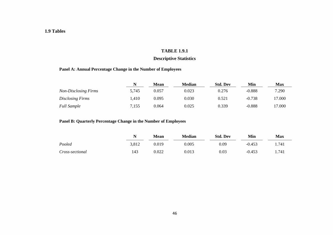
The properties of disclosing firms differ from non-disclosing firms. Panel A of Table
1.9.1 provides descriptive statistics23 for the annual change in the number of employees for all
sample firms. The mean (median) change in the number of employees for the full sample is
6.4% (2.5%). The mean (median) annual change in the number of employees of disclosing
firms is 9.5% (3.0%), while the mean (median) annual change for non-disclosing firms is 5.7%
(2.3%). The mean change in the number of employees of disclosing firms is statistically
significantly higher than the mean change of non-disclosing firms (t=3.804).24 This suggests
that disclosing firms change their workforce more abruptly from one year to the next.
Panel B of Table 1.9.1 presents the descriptive statistic for the quarterly change in the
number of employees for disclosing firms. The mean (median) firm-quarter change (pooled)
21 Companies start filling through EDGAR in 1994. 22 At least two consecutive quarters. 23 The annual number of employees and the quarterly and annual financial data are from Compustat. 24 A nonparametric test, Wilcoxon-Mann-Whitney, suggests that the underlying distributions of the two
samples are statistically significant different (Z=2.803).
26
in the number of employees is 1.9% (0.5%), and the mean (median) firm increases its
workforce by 2.2% (1.3%) per quarter on average (cross-sectional). The quarterly change in
employment is more volatile than the average cross-sectional change (variance of 0.009 and
0.003, respectively), implying that employment fluctuates more across firms than within firms.
The maximum (minimum) quarterly change is 174.1% (–45.3%), suggesting that changes in
employment may reflect acquisition and divesting activities.
The decision to disclose appears to be associated with industry membership. Table
1.9.2 presents the number of firms in the full sample and the number of disclosing firms by
industry division (SIC). Voluntary employment disclosures are most common for firms in
finance, insurance, and real estate (36% of the sample firms) and in services (32%). These
industries rely on human capital for their operations and may use these disclosures to provide
investors with information regarding their current level of economic activity and prospects.
Furthermore, banks are required to disclose their workforce size on form Y-9C, which
all banks with assets greater than $500 million must file with the Federal Reserve quarterly.
This regulatory requirement may explain why financial institutions are more likely to provide
quarterly disclosures regarding their labor force. Financial institutions also have a business
model that differs substantially from firms in other industries. Thus, I exclude banks and
financial institutions (SIC codes between 6000 and 6500) from the main analyses.
I proceed by examining changes in the firms’ employment disclosure policy. Figure
1.8.1 describes the number of firms that change their disclosure policy between 1994 and 2016.
I define a firm-quarter t as a “Start Disclosure” quarter, if the firm discloses its workforce size
in quarter t but does not disclose information about its workforce size in quarter t-1. Similar,
a “Stop Disclosure” quarter is defined as a quarter in which the firm does not disclose
information about employment, although in the prior quarter t-1, the firm provides information
on its workforce size.
27
Figure 1.8.1 shows that more firms initiate employment disclosure during the sample
period. In general, it appears that over time, more firms start providing employment
disclosures than stop providing such disclosures. The difference between the number of firms
that start disclosing and the number of firms that stop disclosing in each period, is positive on
average. During the sample period, 2006-2016, the difference between the number of firms
that start providing employment disclosures and stop providing these disclosures in each
quarter, is 0.659 on average (statistically significant different from zero at a 10% level).
Extending the time period to 1994, the average difference is 0.772 (statistically significant
different from zero at a 1% level).
The main analysis and remaining tests use both disclosing and non-disclosing firms.
I use the Heckman (1979) procedure to correct for potential sample selection bias from the
nonrandom choice of providing quarterly disclosures. I estimate a selection model for firm i
at time t, using the full sample and construct the inverse Mills ratio. The selection model is as
follows.
All variables are defined in Appendix 1.7.1.
The dependent variable (Disclose) is an indicator variable equal to 1 if the firm
provides voluntarily employment disclosure for the fiscal quarter t, and 0 otherwise. In my
sample,25 firms that choose to disclose quarterly have, on average, higher market
capitalization, more assets, and are more likely to belong to the high-tech industry.26 Thus I
expect the likelihood of disclosing the number of employees quarterly (Pr(𝐷𝑖𝑠𝑐𝑙𝑜𝑠𝑒)) to
increase with total assets (TotalAssets) and market value of equity (MVE). Furthermore, as
25 In sections 1.4 and 1.5, I further discuss the characteristics of disclosing and non-disclosing firms. 26 I follow Kasznik and Lev’s (1995) classification of high-technology industries. A firm is classified
as high-tech if it is a member of pharmaceuticals (SIC codes 2833–2836), R&D services (8731–8734),
programming (7371–7379), computers (3570–3577), or electronics (3600–3674) industries.
I report p-values in italics and *, **, and *** denote statistical significance at the 10%, 5%, and 1% (two-tail) levels, respectively.
Regression with time and industry fixed effects. Robust standard errors corrected for heteroskedasticity and autocorrelation using the Newey-
West procedure.
54
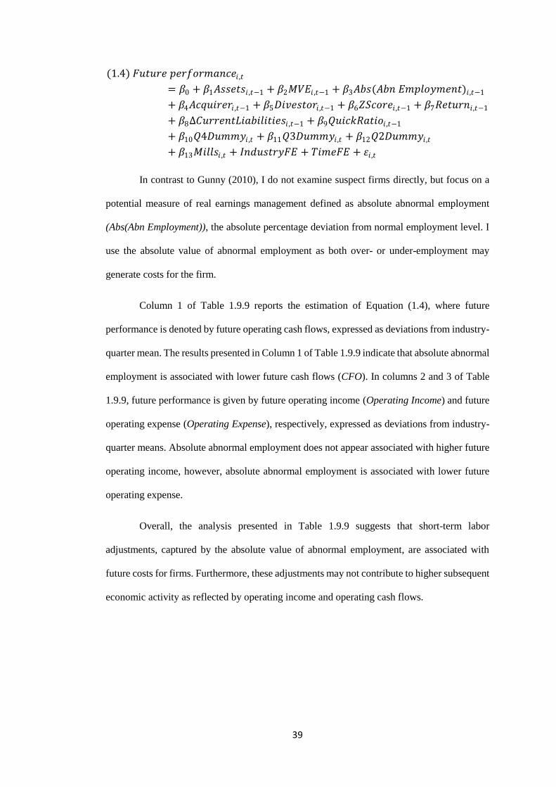
TABLE 1.9.9
Regression Results: Future Performance
(1) CFOt+1
(2) Operating
Incomet+1
(3) Operating
Expenset+1
Intercept 0.064 -0.033 0.146
0.350 0.329 0.157
Assetst -0.012** -0.001 -0.005
0.024 0.702 0.407
MVEt 0.000*** 0.000** -0.000**
0.006 0.021 0.036
Abs(Abn Employment)t -0.052** -0.015 0.169**
0.020 0.204 0.042
Acquirert -0.018** -0.010** -0.041***
0.042 0.014 0.000
Divestort 0.023* -0.023 0.040
0.074 0.406 0.324
ZScoret 0.018*** 0.013*** 0.021***
0.000 0.000 0.001
Returnt 0.019** 0.009** 0.013
0.043 0.013 0.128
ΔCurrentLiabilitiest -0.004 -0.015 0.015
0.922 0.324 0.703
QuickRatiot -0.003 -0.002* -0.007**
0.138 0.067 0.038
Q4Dummyt+1 0.096*** 0.002 0.014**
0.000 0.182 0.014
Q3Dummyt+1 0.052*** 0.002 -0.001
0.000 0.117 0.874
Q2Dummyt+1 0.024*** 0.000 -0.004
0.000 0.956 0.437
Millst+1 -0.030 0.019 -0.051
0.138 0.112 0.237
Industry Fixed Effects Yes Yes Yes
Time Fixed Effects Yes Yes Yes
N 1,960 1,931 1,956
Adjusted R2 0.436 0.420 0.592
I report p-values in italics and *, **, and *** denote statistical significance at the 10%, 5%, and
1% (two-tail) levels, respectively. Standard errors are clustered at the firm level. All continuous
variables are winsorized at the 1% and 99% level.
55
TABLE 1.9.10
Regression Results: Probability of Just Meeting or Beating Earnings
Benchmarks
Pr(Small earnings)
Pr(ΔEarnings)
Pr(Analyst
consensus)
Intercept -7.828*** -6.177*** -1.457
0.000 0.000 0.121
Discloset 0.133 0.227*** 0.293***
0.548 0.001 0.001
Assetst 0.732*** 0.162*** -0.054
0.000 0.000 0.117
HabitualBeatert 2.066*** 0.533*** 1.775***
0.004 0.000 0.000
QuickRatiot 0.031 0.002 -0.034
0.193 0.915 0.184
ΔCurrentLiabilitiest -0.199 -0.171*** 0.067
0.316 0.005 0.201
MVEt -0.000*** -0.000*** 0.000***
0.000 0.009 0.002
ZScoret -0.103*** 0.061*** 0.047**
0.000 0.001 0.027
Q4Dummyt -0.097 -0.048 -0.025
0.684 0.542 0.790
Q3Dummyt -0.507** 0.290*** 0.001
0.045 0.000 0.988
Q2Dummyt -0.230 0.341*** -0.033
0.373 0.000 0.734
Millst 0.491 0.420*** -0.442**
0.355 0.004 0.012
Industry Fixed Effects Yes Yes Yes
Time Fixed Effects Yes Yes Yes
N 20,289 20,289 20,289
Pseudo R2 0.118 0.044 0.059
I report p-values in italics and *, **, and *** denote statistical significance at the 10%, 5%, and
1% (two-tail) levels, respectively. Robust standard errors. All continuous variables are winsorized
at the 1% and 99% level.
56
Chapter 2
IFRS Adoption and Litigation Risk: Evidence from Directors’
and Officers’ Liability Insurance
Brian M. Burnett
Daphne Hart
Paige H. Patrick
2.1 Introduction
As more countries adopt more principles-based accounting standards, such as
International Financial Reporting Standards (IFRS), it becomes increasingly important to
understand the costs and benefits of such standards. Regulators argue that transitioning to more
principles-based standards leads to benefits, including improvement in financial reporting quality,
increased comparability across countries, and improved alignment among shareholders, auditors,
and reporting firms (e.g., SEC 2003). Empirical research documents such positive outcomes when
European firms adopt IFRS (e.g., Barth et al. 2008, Daske et al. 2008, Armstrong et al. 2010,
Brüggemann et al. 2013). However, individual firms incur costs associated with IFRS adoption,
such as transition costs and increases in audit fees (e.g., Kim et al. 2012, De George et al. 2013).
*We appreciate the comments of Vasiliki Athanasakou, Hong Kim Duong (discussant), Bjorn Jorgensen,
Wim Van der Stede, and seminar participants at the 2017 IE Doctoral Consortium, London School of
Economics and Political Science, Tel Aviv University, the 2018 International Accounting Section Midyear
conference, the 41st EAA Annual Congress and the 2018 AAA Annual Meeting. We thank Alexander
Barrett and Rani Suleman for excellent research assistance.
57
We extend the discussion of the costs and benefits of principles-based accounting standards by
investigating whether litigation risk changes upon adoption of more principles-based accounting
standards.
To understand the effect of principles-based accounting standards on litigation risk, we
study changes in two established proxies for litigation risk, Directors' and Officers' (D&O)
liability insurance and excess cash holdings (Core 1997, Core 2000, Chung and Wynn 2008, Wynn
2008), around the adoption of IFRS in Canada. D&O liability insurance policies are corporate
insurance policies that are purchased by firms and cover the firms’ directors and officers.1 Firms
may also hold cash as a form of self-insurance (Wynn 2008). For firms that carry D&O insurance,
excess cash available for indemnification may be used as an additional cushion in case of
litigation, while for firms that do not carry D&O insurance, excess cash may substitute for
insurance.
We investigate changes in litigation risk in Canadian firms for several reasons. First,
Canadian firms face relatively high levels of litigation risk, probably only second to US firms.
Second, unlike US firms, public Canadian firms are required to disclose whether they purchase
D&O liability insurance, and these disclosures often include information about the insurance
premium and coverage limit. Third, Core (1997) finds meaningful variation in the proportion of
Canadian firms that purchase D&O insurance. In his sample, two-thirds of firms carry D&O
insurance, whereas more than 90% of US firms carry D&O insurance.
In addition, Canada offers a natural setting for empirical-archival studies of the effects of
adopting more principles-based accounting standards. Canada switched its reporting standards
from Canadian Generally Accepted Accounting Principles (GAAP) to IFRS for fiscal years
starting on or after 1 January 2011. Pre-IFRS Canadian GAAP was close to US GAAP
(Bandyopadhyay, Hanna and Richardson 1994, Cormier and Magnan 2016), which is considered
1 We discuss the details of D&O liability insurance in greater detail in Section 2.2.
58
a more rules-based standard.2,3 Furthermore, IFRS adoption in Canada was not accompanied by
other significant changes to the regulatory environment or enforcement intensity that would
otherwise confound our inferences.
Ex ante, whether or how Canadian IFRS adoption affects litigation risk is unclear. On the
one hand, litigation risk may be higher once Canadian firms adopt IFRS. Lack of specific rules
means managers will have to rely more on their own judgment, which could result in more legal
challenges to their decisions (Hail et al. 2010, Donelson et al. 2012). Furthermore, the additional
discretion and relative lack of guidance may allow managers to engage in more opportunistic
behavior (e.g., Nelson et al. 2002, Donelson et al. 2016), which would likely result in an increase
in firms’ litigation risk.
On the other hand, IFRS adoption may reduce litigation risk relative to pre-IFRS Canadian
GAAP. As IFRS provides less guidance, it could reduce the occurrence of transaction structuring
to obtain specific accounting treatment (Nelson et al. 2002, Ewert and Wagenhofer 2005, Hail et
al. 2010). Moreover, if IFRS adoption improves financial reporting quality or allows for the less
costly dissemination of private information as some suggest (e.g., SEC 2003, Hail et al. 2010,
Joos and Leung 2013), the occurrence of lawsuits and their expected costs should decrease
accordingly. IFRS may permit firms to produce financial statements that are more informative and
better represent the firm’s financial standing, thus, IFRS adoption may reduce firms’ litigation
risk.
2 While US GAAP is considered a more rules-based standard, pre-IFRS Canadian GAAP is considered a
more principles-based standard. However, pre-IFRS Canadian GAAP is relatively more rules-based than
IFRS, largely due to harmonization efforts with US GAAP. Prior to 2004, a primary objective of the
Canadian’s Accounting Standards Board’s (AcSB) was to minimize differences from US GAAP
(Discussion Paper of Accounting Standards in Canada: Future Directions June 24, 2004). Each year the
AcSB performed a detailed review of differences between Canadian GAAP and US GAAP for a random
sample of Canadian firms cross-listed in the US that reported reconciliations from Canadian GAAP to US
GAAP. The AcSB then developed standards that eliminated or minimized these differences. 3 Cormier and Magnan (2016) note that, while a full-fledged convergence between Canadian GAAP and
US GAAP took place around the mid-1990s, Canadian accountants and auditors may have applied the
standards differently than their US counterparts due to the more principles-based approach in Canada.
59
To examine the effect of IFRS adoption on litigation risk, we hand-collected D&O
insurance data for all firms listed on the Toronto Stock Exchange (TSX) with available Compustat
data. Following Core (1997, 2000), Chung and Wynn (2008) and Wynn (2008), we analyze
changes in perceived litigation risk using four proxies for litigation risk: D&O coverage limit,
D&O premiums, the premium-to-coverage ratio, and excess cash holdings.
In our first set of analyses, we find mixed evidence of the effect of IFRS adoption on
litigation risk. For non-cross-listed Canadian firms, we show that D&O insurance premiums, the
premium-to-coverage ratio and excess cash holdings decreased around IFRS adoption, consistent
with a decrease in litigation risk. However, we find that D&O insurance coverage increased,
suggesting an increase in litigation risk. Kim (2015) finds that high-tech firms have lower
coverage limits and posits that the high premiums charged to these firms result in reduced
coverage limits. Thus, we interpret the combination of increases in coverage limits and decreases
in premiums, along with reductions in the price per unit of insurance as evidence consistent with
a decrease in litigation risk. The reduction in excess cash holdings provides additional support to
our interpretation.
In our second set of analyses, we separately study Canadian firms that are cross-listed on
US exchanges. Canadian firms cross-listed in the US were permitted to report under either
Canadian GAAP or US GAAP prior to the mandated IFRS adoption, but after January 2011, these
firms were permitted to report under IFRS or US GAAP (Burnett et al. 2015). We focus on
Canadian firms cross-listed in the US that switched from Canadian GAAP to IFRS and document
a reduction in D&O insurance premiums, premium-to-coverage ratio and excess cash holdings,
whereas D&O insurance coverage is unchanged. The results from this analysis are consistent with
a reduction in litigation risk.
While cross-listing in the US may lead to higher exposure to litigation risk, litigation and
enforcement efforts in the US were likely unaffected by IFRS adoption in Canada. As such, our
60
second set of analysis provides additional evidence that our main results are not driven by changes
in enforcement in Canada that were concurrent with IFRS adoption.
We also conduct a difference-in-differences analysis comparing changes in litigation risk
of Canadian firms that are cross-listed in the US to those of New York State incorporated (NY)
firms. The difference-in-differences analysis allows us to further control for confounding effects.
We use NY firms as a control group because these firms are required to disclose information about
their D&O insurance policies and continuously report under US GAAP. NY firms always reported
under a rules-based system, while some Canadian firms cross-listed in the US adopted a more
principles-based system after January 2011.We document that the insurance coverage for those
cross-listed firms that switched to IFRS decreased relative to NY firms that always report under
US GAAP. The reduction in insurance coverage is consistent with lower litigation risk following
IFRS adoption.
Overall, we find evidence that IFRS adoption decreases litigation risk. This is contrary to
the results in Donelson et al. (2012) who find that principles-based standards result in greater
litigation risk. Our study differs substantially from theirs: we utilize proxies for expected
litigation, rather than litigation outcomes. Moreover, Donelson et al. (2012) exploit variation in
the extent to which US GAAP standards are rules- or principles-based, while we focus on an
externally mandated change from a more rules-based accounting standard to a more principles-
based standard, rather than variation among standards at a point in time.
Our findings should be of interest to regulators and investors. We document that
modifications of accounting regulations alter litigation risk, as measured by the cost of D&O
insurance and excess cash holdings. We contribute to the understanding of the costs and benefits
associated with adopting a more rules-based standard, such as IFRS. Our results may also inform
policy debates in the US on the effects of adopting more principle-based standards.
The rest of the chapter is organized as follows. Section 2.2 describes D&O insurance
contract and the related literature. Section 2.3 develops the hypotheses and section 2.4 discusses
61
the research design. Section 2.5 presents the main analysis results. We conduct robustness tests in
Section 2.6 and conclude in Section 2.7. All variables are defined in Appendix 2.8.1.
2.2 Directors’ and Officers’ (D&O) Liability Insurance
In this section, we review prior literature documenting an association between D&O
insurance and firm characteristics and corporate governance as well as shareholders’ and
insurance providers’ risk assessment.
Directors’ and officers’ liability insurance is a contract between a firm and an insurance
company. Although the firm purchases and owns the insurance policy, the firm’s directors and
officers are the beneficiaries of the policy. In the event directors or officers are named as
defendants in a lawsuit related to their duties, the D&O liability insurance provider either
reimburses the directors and officers directly for all the associated expenses (provided directors
acted in good faith and met the applicable standard of conduct), or the firm indemnifies the
directors and officers for their expenses, and then claims the expenses from the insurance provider.
D&O liability insurance contracts specify the quantity and the price of insurance, as
agreed by both the insurance provider and the firm. The coverage limit (quantity) is the maximum
dollar value of the D&O insurance policy. The coverage limit is the maximum amount the
insurance provider may be liable for and as such, is an assessment of the aggregate potential costs
of litigation given the insurance premium (price). D&O insurance premium is the total cost of the
insurance policy, which represents an estimation of the likelihood of litigation and its expected
costs, with a markup for the insurer. As insurance institutions perform risk sharing and risk
management functions efficiently (Cummins 1991), insurance contracts, in general, are
informative about firms' risk exposures.
Prior literature demonstrates that D&O insurance reflects firm-level litigation risk. Using
a sample of public Canadian firms, Core (1997) documents that firms with greater litigation risk
and higher distress probability are more likely to purchase D&O insurance and carry higher
62
coverage limits. Further, Core (2000) uses D&O liability insurance as a measure of ex-ante
litigation risk and demonstrates that weaker governance is associated with higher premiums and
excess CEO compensation. O’Sullivan (2002) finds similar results for public UK firms:
companies carrying D&O insurance tend to be larger and associated with greater likelihood of
litigation, greater proportions of non-executive board members, and less managerial ownership.
D&O insurance reflects the firm’s as well as the insurer’s expected litigation risk. Gillan
and Panasian (2015) argue that D&O insurance limits and premiums appear informative about the
firm specific probability of lawsuits and governance quality. Furthermore, Cao and
Narayanamoorthy (2014) view the insurance premiums charged as indicative for the insurers’
assessment of the firm’s litigation risk. For a sample of public US firms, they show that firms with
prior accounting restatements or lower earnings quality, pay higher premiums. These results are
consistent with Lin et al. (2013) who detect a positive association between D&O coverage and
earnings restatements.
Prior literature also argues that D&O insurance is used to improve corporate governance
and protect shareholders. Holderness (1990) emphasizes the role of D&O insurance as a
mechanism to monitor executives. O’Sullivan (1997) argues that, as firm size increases, external
ownership becomes a costly monitoring scheme. He shows that larger public UK firms are more
likely to utilize outside directors and D&O insurance to monitor executives.
In related work, Boyer (2014) provides empirical evidence suggesting that shareholders
use D&O insurance to protect their own wealth in case of managerial incompetence. The more
shareholders have at risk, the larger the insurance protection. Moreover, Caskey (2014) illustrates
analytically that while carrying D&O insurance increases the likelihood of litigation, the insurance
also partly alleviates investors' incorporation of the potential litigation costs into the stock price.
Thus, D&O insurance may reduce expected costs and overall, increase firm value.
To the extent that legal liability insurance alters managers' behavior, D&O insurance and
litigation risk are interdependent (Pauly 1974, Holmstrom 1979). Wynn (2008) hypothesizes that
63
excess D&O insurance and excess cash available for indemnification are primary determinants of
firms' disclosure policy. She studies a sample of Canadian firms and document a negative
association between exposure to litigation risk and legal liability coverage, and the timeliness of
bad news disclosures and the frequency of bed news forecasts. Moreover, managers with higher
legal liability coverage tend to disclose bad news more precisely.
D&O insurance also reflects managers’ private information about expected firm
performance. Chalmers, Dann and Harford (2002) study D&O insurance around US initial public
offerings (IPOs) and find that D&O insurance premiums are positively related to IPO size and
negatively related to leverage, the percentage sold by venture capitalists, and the average operating
income. Moreover, Chalmers et al. (2002) document a significant negative relation between the
three-year post-IPO stock price performance and the insurance coverage purchased in conjunction
with the IPO, which suggests the coverage limits are set opportunistically prior to IPOs. In
contrast, Boyer and Stern (2014) study Canadian IPOs and find that insurance providers charge
higher premium per dollar of coverage to firms with poor stock performance, higher volatility and
lower Sharpe ratios post-IPO. Boyer and Stern’s (2014) results indicate that in their setting,
insurers have superior information relative to investors.
Prior literature proposes that D&O insurance is associated with managerial entrenchment
and affect risk-taking incentives. Core (1997) argues that entrenched managers demand higher
levels of D&O insurance. Consistent with this argument, Chung, Hillegeist and Wynn (2015) use
D&O liability insurance to construct a proxy for managerial opportunism and document a positive
association between excess D&O insurance coverage and audit fees. Lin et al. (2011) present
evidence of an association between D&O insurance and real decisions. For a sample of publicly
traded Canadian firms, they show that managers of firms carrying high D&O insurance coverage
limits make poor M&A decisions. Particularly, those managers pay higher premiums for their
acquisitions and their acquisitions exhibit lower synergies. Lin et al. (2011) conclude that acquirer
firms with high levels of D&O insurance generate lower returns for their stockholders, indicating
64
those firms’ managers are more inclined to risk taking and are less sensitive to shareholder
discipline. Furthermore, Lin et al. (2013) document a positive relation between D&O insurance
levels and loan spreads, suggesting that lenders associate higher D&O insurance limits with
greater risk taking. Similarly, Chen, Li and Zou (2016) show that D&O insurance limits are
positively associated with the ex-ante cost of capital as implied by stock prices and analyst
forecasts.
2.3 Hypothesis Development
A more principles-based accounting standard may require the exercise of additional
managerial discretion and professional judgment relative to a more rules-based accounting
standard. The effect of increased discretion on litigation risk has been debated. Schipper (2003)
raises the concern that principles-based standards result in greater expected litigation costs,
whereas the SEC (2003) predicts lower litigation costs.
On the one hand, litigation risk may be higher under more principles-based accounting
standards than under more rules-based accounting standards. Rules provide a “safe harbor”, which
protects firms from litigation (Schipper 2003, Donelson et al. 2012). Lack of specific rules means
managers will necessarily rely more on their own judgment, which could result in more legal
challenges to their decisions (Hail et al. 2010). Moreover, additional discretion and less guidance
may affect managers’ opportunistic behavior. Nelson et al. (2002) show that imprecise standards
are associated with more earnings management via discretion in accounting judgments than are
precise standards. An increase in opportunistic financial reporting would likely result in an
increase in firms’ litigation risk. While prior research does not find significant changes in earnings
quality around IFRS adoption in Canada (e.g., Burnett et al. 2015, Liu and Sun 2015), IFRS
adoption may still alter litigation risk if it facilitates opportunistic behavior.
On the other hand, adoption of more principles-based accounting standards such as IFRS
may reduce litigation risk. Donelson et al. (2012) also propose that rules-based systems provide
65
shareholders a “road map” for potential litigation. They argue that violations of clear guidance are
likely to be intentional, and therefore, litigation outcomes are more likely to favor plaintiffs. As
IFRS provides less guidance, it could also reduce the occurrence of transaction structuring to
obtain specific accounting treatment (Nelson et al. 2002, Ewert and Wagenhofer 2005, Hail et al.
2010). Similarly, Joos and Leung (2013) argue that more principles-based accounting standards
have fewer bright-line rules and are considered less complex. Thus, principles-based standards
may allow firms to better balance between complying with accounting standards and producing
financial reports that reflect firms’ underlying economics.
Furthermore, the SEC (2003) suggests that the joint implementation of principles-based
standards and effective enforcement, better aligns incentives among auditors, reporting firms, and
investors, which increases reporting quality and decreases litigation costs. Finally, the additional
managerial discretion required under IFRS, enables managers to convey private information to
the markets in a more effective and less costly fashion (Hail et al. 2010). Consistent with these
predictions, Cormier and Magnan (2016) document an increase in value relevance for Canadian
firms cross-listed in the US that adopt IFRS. In sum, if IFRS permits firms to produce financial
statement that are more informative and better represent the firm’s financial standing, it may
reduce the occurrence and expected costs of lawsuits.
Scant empirical research investigates the association of litigation risk with rules-based
versus principles-based accounting standards. Donelson et al. (2012) find evidence suggesting that
more rules-based accounting standards reduce the threat of litigation. They document that
restatements involving a violation of rules-based standards are associated with a lower probability
of litigation. Moreover, they show that when firms are sued with no prior related restatement,
plaintiffs are more likely to allege a violation of principles-based standards. Donelson et al. (2016)
investigate why US accounting standards take on more rules-based characteristics. They find that
both cross-sectional and time-series variation in rules-based characteristics of US GAAP are
related to changes in litigation risk and to changes in the complexity of the underlying transaction
66
and accounting treatment. The empirical findings in Donelson et al. (2012, 2016) suggest that
more principle-based standards are associated with higher litigation risk, thus, switching from
Canadian GAAP to IFRS would be associated with increased litigation risk.
A related stream of literature investigates audit fees around IFRS adoption. Audit fees
capture the auditor’s assessment of the firm's litigation risk while D&O insurance captures the
firm's individual risk. IFRS adoption may alter audit fees due to changes in financial reporting
incentives affecting earnings quality, or because of changes in litigation risk.4 Kim et al. (2012)
find that European Union firms’ audit fees increased by 5.4 percent around IFRS adoption in 2005.
They show that IFRS-related audit fee premiums increase with the audit complexity introduced
by IFRS adoption but decrease with the improvement in financial reporting quality arising from
IFRS adoption. De George et al. (2013) find similar results for Australian firms. They document
an increase in audit fees around IFRS adoption and argue that average audit fees increase in excess
of 8 percent beyond the normal annual fee growth in the pre-IFRS adoption period.
Overall, prior literature finds that audit fees increase around IFRS adoption. This increase
is consistent with higher litigation risk following IFRS adoption. Nevertheless, as auditors are
likely to increase audit effort to manage the risk of IFRS adoption (De George et al. 2013), audit
quality may improve, inducing a decrease in litigation risk. Thus, the documented increase in audit
fees may also be consistent with lower litigation risk following IFRS adoption.
Collectively, the above arguments and corresponding empirical evidence suggest that the
association between IFRS adoption and ex-ante perceived litigation risk may be either positive or
negative. On the one hand, switching to IFRS may increase legal exposure by eliminating the
shield provided to Canadian firms by the more explicit rules and guidance in Canadian GAAP.
On the other hand, IFRS adoption may facilitate transferring private information from managers
4 Examining D&O liability insurance around IFRS adoptions extends prior literature and provides another
perspective on the costs and benefits of IFRS adoption for individual firms.
67
to investor and producing financial statements that better reflect the firm’s underlying economics.
This leads to our formal hypothesis (stated in the null form):
H: IFRS adoption does not affect perceived litigation risk.
2.4 Research Design
2.4.1 The Canadian Setting
Canada offers a natural setting for empirical-archival studies of the effects of adopting a
more principle-based accounting standard on litigation risk. First, public Canadian firms are
required to disclose whether they purchase D&O liability insurance, and these disclosures often
specify the cost and terms of the insurance contract. We use the information regarding the cost
and terms of the insurance contracts to measure perceived litigation risk at the firm level.
Second, Canada switched its reporting standards from Canadian GAAP to IFRS for fiscal
years starting on or after 1 January 2011. Prior to 2011, most Canadian public firms reported using
Canadian GAAP. While Canadian GAAP is a principles-based standard, it provides more detailed,
rules-oriented guidance than does IFRS.5 Thus, the Canadian setting permits examining whether
more detailed accounting guidance influences either the incidence or the cost of litigation.
Moreover, IFRS adoption in Canada took place in a period that follows the introduction
of strengthened corporate governance requirements, such as the National Instrument 52-109 which
became effective in Canada in 2008 (Lu et al. 2011) and the Sarbanes-Oxley Act of 2002, in the
US, which was effective for Canadian firms cross-listed in the US from 2007. Our sample period
has consistently high levels of enforcement throughout, and we are unaware of any significant
changes to enforcement or regulation that coincide with IFRS adoption in Canada.
5 Prior to 2004 the Canadian Accounting Standards Board (AcSB) was actively implementing a strategy of
harmonizing Canadian GAAP with US GAAP. Each year it reviewed US-cross-listed firms' reconciliations
between Canadian GAAP and US GAAP and worked on revising standards to minimize these differences.
68
2.4.2 Canadian Firms Cross-listed in the US
Since IFRS adoption in Canada is clustered in time, other events that took place around
2011 may have altered firms’ litigation risk and any observed association between IFRS adoption
and litigation risk is due to alternative explanations.6 We address this concern in two ways. First,
we examine Canadian firms cross-listed in the US that adopted IFRS. These firms operate in the
US, which was likely unaffected by the accounting standard change in Canada or other regulatory
and enforcement acts that happened in Canada around 2011. Second, we compare the costs of
D&O insurance for Canadian firms cross-listed in the US and US firms incorporated in the state
of New York.
The US is considered more litigious than Canada. Hence, the sample of Canadian firms
cross-listed in the US permits examining the effect of adopting IFRS in a more litigious country
while using D&O insurance information as a proxy for litigation risk and holding fixed the
disclosure requirements.
Under the Multi-Jurisdictional Disclosure System (MJDS) adopted in 1991, Canada and
the US permit Canadian (US) firms to access US (Canadian) capital markets using prospectuses
prepared in accordance with Canadian (US) disclosure requirements. Hence, Canadian firms can
access US capital markets with limited oversight from the SEC (Burnett et al. 2017) and without
additional disclosure requirements.
Moreover, prior to IFRS adoption in 2011, Canadian firms cross-listed in the US were
permitted to choose between Canadian GAAP and US GAAP, and, firms reporting under
Canadian GAAP were exempted from the requirement to reconcile to US GAAP (Burnett et al.
2017). After Canada adopted IFRS in 2011, Canadian firms cross-listed in the US were permitted
to prepare their financial statements in accordance with IFRS or US GAAP. As the SEC exempted
6 See for example Christensen, Hail and Leuz (2013), which suggests that capital market benefits of IFRS
adoption are driven by increased enforcement that coincide with IFRS adoption periods.
69
all non-US firms reporting under IFRS from reconciliation to US GAAP, Canadian firms that
choose to adopt IFRS maintained the exemption from the reconciliation requirement.
While information about D&O insurance is not generally publicly disclosed by US firms
(Griffith 2006), Canadian firms cross-listed in the US do provide information7 regarding their
indemnification policy and D&O insurance as required by the Canada Business Corporations Act.8
This mandatory disclosure requirement of D&O insurance information allows us to a measure
perceived litigation risk for Canadian firms cross-listed in the US.
We also use NY firms as a control group for Canadian firms cross-listed in the US in a
difference-indifferences research design. New York Business Corporation Law mandates public
firms incorporated in New York State to disclose their D&O insurance policy information to their
shareholders.9 Thus, similar to Canadian firms, NY firms are required to disclose whether they
purchase D&O insurance policy. Furthermore, they are required to specify the insurance costs.
Unlike the sample of Canadian firms cross-listed in the US, NY firms did not change their
accounting standard during the sample period - these firms always report under US GAAP.
2.4.3 Specifications
Our main variable of interest is 𝑃𝑂𝑆𝑇𝑡, defined as 1 if a firm reports under IFRS at time
𝑡, and 0 otherwise. We are interested in the effect of IFRS adoption (POST) on litigation risk and
use three proxies for litigation risk for firms with D&O liability insurance: the insurance coverage
limit, insurance premiums, and the premium-to-coverage ratio. If IFRS adoption increases
(decreases) a firm’s litigation risk, the coefficient on POST will be positive (negative).
First, D&O insurance coverage (COVERAGE), the log of the maximum amount D&O
insurance provider may be liable for, is used as a proxy for litigation risk where, ceteris paribus,
7 We exclude US firms cross-listed in Canada from our sample, as these firms are not required to disclose
whether they carry D&O insurance. 8 Canada Business Corporations Act (CBCA) - R.S.C., 1985, c. C-44 (Section 124). 9 New York Business Corporation Law, Article 7, Section 726.
16 In Column 1 Table 2.9.4, the depended variable is the natural logarithm of D&O coverage limit and the
independent variable POST is a dummy variable. We note that exp(0.14) = 1.1503, thus the percentage
change in D&O coverage limit post-IFRS adoption is 15.03%. 17 We note that exp(-0.09) = 0.914 and exp(-0.12) = 0.887. 18 The average premium-to-coverage ratio pre-IFRS adoption is 0.005 (see Table 2.9.2). The average
premium-to-coverage ratio decreases by 0.0005 post-IFRS adoption, implying that for the average firms,
the premium-to-coverage declines by 10%.
80
that to some extent, litigation risk diminishes around IFRS-adoption for Canadian firms not cross-
listed in the US.
Table 2.9.6 reports our regression analyses for firms that are cross-listed in the US. In
column 1 of Table 2.9.6, we examine D&O coverage limit and do not find that coverage limits
change around IFRS adoption. Thus, we cannot reject the null that IFRS adoption does not affect
litigation risk as captured by the D&O liability insurance coverage limits. As expected, the
coefficients on SIZE, HIGHTECH and VOLATILITY are positive and statistically significant. The
significant coefficient on QUEBEC indicates that firms headquartered in Quebec have
substantially lower coverage limits relative to firms headquartered in the rest of Canada.
Column 2 and column 3 of Table 2.9.6 suggest that D&O premium decreases for firms
cross-listed in the US post-IFRS adoption, which is consistent with our analysis for firms not
cross-listed in the US. The negative and statistically significant coefficients on POST indicate that
D&O premium decreases by 11.3-17.3% post-IFRS adoption.
Based on column 3 of Table 2.9.5, we note that, for firms cross-listed in the US, divesting
activities (DIVESTOR) and more volatile stock returns (VOLATILITY) are associated with higher
D&O premiums. This result is consistent with prior literature (Core 1997). The negative and
statistically coefficient on QUEBEC indicates firms headquartered in Quebec pay lower premiums
consistent with lower litigation risk.
Column 4 of Table 2.9.6 shows the regression results for premium-to-coverage ratio. The
coefficient on POST is negative (-0.0025) and statistically significant (p-value 0.009), implying
that on average, firms pay 25%19 less per dollar of coverage post-IFRS adoption. The positive and
significant coefficient on HIGHTECH is in line with the expectation of a higher cost of D&O
coverage for firms in the higher risk industries.
19 The average premium-to-coverage ratio pre-IFRS adoption is 0.010 (see Table 2.9.2). The average
premium-to-coverage ratio decreases by 0.0025 post-IFRS adoption, implying that for the average firms,
the premium-to-coverage declines by approximately 25%.
81
Collectively, we interpret the multivariate regression analysis presented in Table 2.9.6 as
being consistent with a decrease in litigation risk after US-cross-listed firms adopt IFRS. D&O
underwriters had been pricing D&O insurance for foreign private issuers reporting under IFRS in
US markets for at least four years when cross-listed Canadian firms began reporting under IFRS.
As such, the underwriters would be relatively well informed about the litigation risks associated
with reporting under IFRS and it appears that they assess that risk lower than when Canadian firms
reported under Canadian GAAP. This result should be of interest to US regulators in assessing
potential litigation costs if the US were to ever adopt IFRS.
2.5.3 Regression Analyses of Excess Cash
As D&O insurance may be substitute using cash available for indemnification, we
examine excess cash holdings by firms that do not own D&O insurance policy. Table 2.9.7 reports
our regression analyses for firms that are not cross-listed in the US. The negative and statistically
significant coefficient on POST of -0.06 (p-value 0.001) indicates that excess cash decreases post-
IFRS adoption. As expected, the coefficient on SIZE is positive and statistically significant,
suggesting bigger firms hold more cash available for indemnification. The coefficient on
DEBTRATIO is significant but negative. This may suggest that financial constraints reduce firms’
excess cash holdings.
Table 2.9.8 reports our regression analyses for firms that do not own D&O insurance
policy and that are cross-listed in the US. The coefficient on POST is negative (-0.10) and
statistically significant (p-value 0.043), consistent with firms holding less excess cash post-IFRS
adoption. Similar to our results for non-cross-listed firms, the coefficient on SIZE is positive and
statistically significant and the coefficient on DEBTRATIO is negative and statistically significant.
Table 2.9.8 also indicates that firms involving in acquisitions (AQUIRER) have more excess cash
while firms headquartered in Quebec (QUEBEC) appear to hold less excess cash.
Overall, our multivariate analysis indicates that firms without a D&O insurance policy
hold less excess cash available for indemnification post-IFRS adoption. We document a reduction
82
in excess cash for firms not cross-listed in the US as well as for firms cross-listed in the US. These
results lend additional support to the conjecture that IFRS adoption is associated with a reduction
in litigation risk.
2.6 Robustness Tests
To control for time trends and potential confounding effects, we employ a difference-in-
differences research design using firms incorporated in NY as a control sample. These firms were
likely not affected by the adoption of IFRS in Canada.
US firms incorporated in the state of New York are required to disclose whether they
purchase directors’ and officers’ liability insurance and the premiums they pay if they have
insurance. Note that if these firms have insurance, they are not required to disclose their insurance
coverage limits.
We hand-collect the premium data for US firms in Compustat that are incorporated in
NY. We collect the data for two years before and after the year NY incorporated firms would have
been required to adopt IFRS had they been in Canada based on their fiscal year-end. Twenty-nine
NY firms disclose premium data for two years before and after the pseudo-IFRS adoption date
and have all the necessary data for our analysis. We note that our sample size is comparable to
Linck, Netter and Yang (2009) who document an increase in D&O insurance premiums for NY
firms following Sarbanes-Oxley Act (SOX).
Table 2.9.9 reports descriptive statistics for NY firms in the year prior to their pseudo-
IFRS adoption date, which is the date they would have switched to reporting under IFRS if they
had to follow the Canadian regulation and adopt IFRS in 2011. Their mean (median) D&O
premium is $2.30 million ($0.87 million). When scaled by total assets, the average D&O premium
for NY firms of 0.0007 is similar to Canadian firms cross-listed in the US at 0.0008. The mean
(median) total assets of NY firms is $2,591.5 million ($2,807.4 million) and is similar to Canadian
firms cross-listed in the US at $3,498.2 million ($2,921.9 million).
83
Table 2.9.10 provides the difference-in-differences regression analysis comparing the
premiums of Canadian firms cross-listed in the US to US NY firms. The negative (-0.13) and
statistically significant (p-value 0.087) coefficient on the interaction term POST*IFRS indicates
that the premiums for Canadian firms cross-listed in the US decrease more than for NY firms after
adopting IFRS. Consistent with our cross-sectional analysis, the positive and statistically
significant coefficients on SIZE, VOLATILITY, and HIGHTECH, indicate that larger, more
volatile firms pay higher premiums, and so do firm operating in higher risk industries.
Our analysis indicates that the perceived litigation risk decreased following IFRS
adoption in Canada. The difference-in-differences analysis results are consistent with IFRS
adoption causing the decline in D&O insurance premiums for Canadian firms cross-listed in the
US, and not just a general trend in the D&O market in the US. Canadian firms cross-listed in the
US benefit from a decline of 12.2% in their D&O insurance premiums, equivalent to an average
saving of $0.118M, once they switched to reporting under IFRS.
This result informs US regulators, investors, lawyers, and managers as they continue to
evaluate and monitor the consequences of IFRS adoption if the US ultimately adopts IFRS or
more principles-based standards. Canadian firms cross-listed in the US are arguably the most
similar firms to US firms of any non-US firms. Our evidence is consistent with IFRS decreasing
litigation risk for firms previously reporting using Canadian GAAP, arguably the most similar
accounting standard to US GAAP.
2.7 Conclusion
In this chapter, we study the effect of adoption of more principle-based standards on
litigation risk. Specifically, we investigate changes in perceived litigation risk around the adoption
of IFRS in Canada. To proxy for litigation risk, we focus our analysis on changes in D&O liability
insurance coverage, premiums, and the ratio of premiums-to-coverage. We also examine excess
84
cash holdings available for indemnification by firms that do not own D&O liability insurance
policy.
The IFRS framework places greater reliance on managerial discretion in the preparation
of financial reports and allows managers more flexibility when choosing accounting policies. De
George et al. (2016) state that IFRS can raise concerns about independent verifiability of reported
figures and increase potential for manipulation of financial accounting. The increased managerial
discretion after IFRS adoption has implications for the litigation exposure of firms, especially
during the initial periods when uncertainty about the new accounting regime is relatively high (De
George et al. 2016). The change in the legal environment induced by the accounting standard
change may therefore modify the coverage and premiums of D&O insurance and the amount of
cash firms choose to hold.
Furthermore, we expect IFRS adoption to affect D&O insurance since D&O insurance is
associated with earnings quality as well as with audit fees, both of which were affected by IFRS
adoption (Chung et al. 2015). Prior literature documents change in audit fees around IFRS
adoption (ICAEW 2007, De George et al. 2013, Kim et al. 2012) possibly due to changes in
financial reporting incentives that affect earnings quality, or due to changes in litigation risk.
While converting to IFRS is also likely to affect financial reporting, accounting standards are only
one of the determinants of overall accounting quality (Soderstrom and Sun 2007).
Overall, we document an additional consequence of IFRS adoption, namely the cost of
D&O insurance. We find consistent evidence that perceived litigation risk decreased for Canadian
firms following IFRS adoption for both firms that are not cross-listed in the US, and those that
are. Our analyses suggest that switching to more principles-based standards is associated with a
reduction in the litigation risk of firms and their directors and officers. Our findings should be of
interest to shareholders and regulators as they suggest that modification of accounting regulations
has real effects on litigation risk and litigation costs.
85
One caveat to our analysis is that we cannot rule out the alternative explanation that factors
other than IFRS adoption caused the change in litigation risk. However, our sample period has
consistently high levels of enforcement throughout, and we are unaware of any significant changes
to the regulatory, economic, or governance environments that coincide with IFRS adoption in
Canada. We further address this concern in two ways. First, by focusing on Canadian firms cross-
listed in the US and examining an environment that is likely unaffected by the standard change or
other regulatory and enforcement acts that happened in Canada around 2011. Second, by
employing a difference-in-differences research design where we compare D&O insurance
premiums of Canadian firms cross-listed in the US with a sample of NY incorporated firms that
are also required to disclose information regarding their D&O insurance.
With increasingly dispersed ownership around the world and the rising prominence of
equity ownership, litigation may become a more widespread mechanism for resolving disputes.
One possible avenue for future research on D&O insurance could be to investigate the cross-
country determinants of D&O insurance and the cross-country D&O disclosure requirements. A
natural extension of our paper would be to examine whether the determinants of D&O insurance
differ between countries with more rules-based standards and more principle-based standards.
Moreover, future research may wish to examine the litigation risk of foreign firms cross-listed in
the US, focusing on the ex-post litigation risk reflected in D&O insurance contracts.
86
2.8 Appendix
APPENDIX 2.8.1
Variable Descriptions
COVERAGEt Log of maximum amount the D&O insurance provider may be
liable for at year t
POSTt A year dummy set equal to 1 for fiscal years after IFRS adoption
in Canada, and 0 otherwise. For NY firms, the variable is set equal
to 1 for fiscal years after pseudo-IFRS adoption date (i.e. the date
after which the US firm should have adopted IFRS given its fiscal
year end if it had been a Canadian firm).
SIZEt-1 Log of total assets at the beginning of the fiscal year t
DEBTRATIOt-1 Debt over the sum of debt and market value of equity at the
beginning of the fiscal year t
ACQUIRERt-1 An indicator variable set equal to 1 if in the prior year the book
value of total assets at the end of the fiscal year increases by more
than 25% from the beginning of the fiscal year, and 0 otherwise
DIVESTORt-1 An indicator variable set equal to 1 if in the prior year the book
value of total assets at the end of the fiscal year decreases by more
than 25% from the beginning of the fiscal year, and 0 otherwise
HIGHTECHt-1 An indicator variable set equal to 1 if a firm is a member of
The table presents univariate tests of differences for both non-cross-listed and cross-listed Canadian firms that adopt IFRS. If
indicated, we use the natural logarithm of the raw values. All continuous variables are winsorized at the 1% and 99% level. *,
**, *** denote statistical significance at the 0.10, 0.05, and , 0.01 levels, respectively, based on t-test for the difference in means
and a nonparametric Wilcoxon signed-rank test for the difference in medians.
92
TABLE 2.9.4
Univariate Tests of Changes in Excess Cash After IFRS Adoption for Firms That Do Not Purchase D&O
Insurance
Panel A: Firms Not Cross-listed in the US That Do Not Purchase D&O Insurance
Pre-IFRS
(N=318)
Post-IFRS
(N=318) Difference
Mean Median Mean Median Mean Median
EXCASH -0.02 -0.08 -0.04 -0.07 -0.02 0.01
Panel B: Firms Cross-listed in the US That Do Not Purchase D&O Insurance
Pre-IFRS
(N=82)
Post-IFRS
(N=82) Difference
Mean Median Mean Median Mean Median
EXCASH -0.10 -0.15 -0.17 -0.14 -0.07 0.01
The table presents univariate tests of differences for both non-cross-listed and cross-listed Canadian firms that adopt IFRS and never
purchased D&O insurance. All continuous variables are winsorized at the 1% and 99% level. *, **, *** denote statistical significance
at the 0.10, 0.05, and, 0.01 levels, respectively, based on t-test for the difference in means and a nonparametric Wilcoxon signed-rank
test for the difference in medians.
93
TABLE 2.9.5
Regression of the Effect of IFRS Adoption on D&O Coverage and Premiums
for Canadian Firms Not Cross-listed in the US
(1) (2) (3) (4)
Variable
Predicted
Sign Coverage Premium
Premiu
m
Premium /
Coverage
Intercept 0.76*** -6.06*** -5.59*** 0.0014***
0.000 0.000 0.000 0.000
POST +/- 0.14*** -0.09*** -0.12***
-
0.0005***
0.000 0.002 0.004 0.002
SIZE + 0.41*** 0.16*** 0.49*** 0.0003***
0.000 0.000 0.000 0.004
DEBTRATIO + -0.18 0.47*** 0.27* 0.0018**
0.444 0.010 0.094 0.028
ACQUIRER +/- -0.11 -0.04 -0.11** -0.0002
0.132 0.358 0.023 0.489
DIVESTOR +/- 0.29*** 0.20* 0.45*** 0.0008
0.006 0.052 0.000 0.171
HIGHTECH + 2.68 0.32** 0.47*** 0.0010**
0.111 0.014 0.000 0.037
VOLATILITY + 2.68* 5.82*** 8.10*** 0.0247***
0.095 0.000 0.000 0.002
QUEBEC - -0.17** 0.03 -0.09 0.0002
0.035 0.353 0.104 0.258
EXCASH - 0.27
0.180 COVERAGE 0.76***
0.000 EXADJCOV 0.76***
0.000 Industry
Fixed Effects Yes Yes Yes Yes
No. of
Observations 636 636 636 636
No. of Firms 159 159 159 159
Adjusted R2 66.3% 82.7% 82.6% 6.1%
All continuous variables are winsorized at the 1% and 99% level. *, **, *** denote
statistical significance at the 0.10, 0.05, and 0.01 levels (one-tailed test if a predicted sign,
and two-tailed test if no predicted sign), respectively, based on robust standard errors
clustered by firm.
94
TABLE 2.9.6
Regression of the Effect of IFRS Adoption on D&O Coverage and
Premiums for Canadian Firms Cross-listed in the US
(1) (2) (3) (4)
Variable
Predicted
Sign Coverage Premium Premium
Premium /
Coverage
Intercept 1.35*** -4.93*** -3.62*** 0.0074***
0.001 0.000 0.000 0.000
POST +/- 0.07 -0.19*** -0.12**
-
0.0025***
0.274 0.001 0.031 0.009
SIZE + 0.38*** -0.05 0.40*** -0.0001
0.000 0.360 0.000 0.397
DEBTRATIO + 0.32 -0.20 0.10 0.0019
0.240 0.257 0.365 0.193
ACQUIRER +/- -0.06 0.06 0.03 0.0004
0.629 0.506 0.689 0.651
DIVESTOR +/- 0.20 0.37 0.52* 0.0088
0.562 0.213 0.090 0.171
HIGHTECH + 0.43* 0.18 0.59* 0.0032*
0.066 0.284 0.051 0.095
VOLATILITY + 2.31** 1.40 3.62** 0.01
0.037 0.213 0.034 0.297
QUEBEC - -0.66*** 0.08 -0.66*** -0.0004
0.000 0.311 0.000 0.386
MILLS +/- -0.25 0.29 -0.04 0.0072
0.637 0.636 0.953 0.339
EXCASH + 0.58*
0.067 COVERAGE 1.13***
0.000 EXADJCOV 1.14***
0.000 Industry
Fixed Effects Yes Yes Yes Yes
No. of
Observations 168 168 168 168
No. of Firms 42 42 42 42
Adjusted R2 85.1% 91.5% 90.7% 23.3%
All continuous variables are winsorized at the 1% and 99% level. *, **, *** denote
statistical significance at the 0.10, 0.05, and 0.01 levels (one-tailed test if a predicted
sign, and two-tailed test if no predicted sign), respectively, based on robust standard
errors clustered by firm.
95
TABLE 2.9.7
Regression of the Effect of IFRS Adoption on Excess Cash for Canadian Firms
Not Cross-listed in the US That Do Not Purchase D&O Insurance
Variable
Predicted
Sign EXCASH Intercept -0.32***
0.000 POST +/- -0.06***
0.001 SIZE + 0.06***
0.000 DEBTRATIO + -0.26***
0.000 ACQUIRER +/- 0.03
0.140 DIVESTOR +/- 0.10
0.121 HIGHTECH + 0.01
0.458 VOLATILITY + -0.37
0.200 QUEBEC - -0.05
0.147 Industry Fixed Effects Yes No. of Observations 636 No. of Firms 159 Adjusted R2 15.4%
All continuous variables are winsorized at the 1% and 99% level. *, **, *** denote
statistical significance at the 0.10, 0.05, and 0.01 levels (one-tailed test if a predicted sign,
and two-tailed test if no predicted sign), respectively, based on robust standard errors
clustered by firm.
96
TABLE 2.9.8
Regression of the Effect of IFRS Adoption on Excess Cash for Canadian
Firms Cross-listed in the US That Do Not Purchase D&O Insurance
Variable
Predicted
Sign EXCASH
Intercept -0.28
0.246 POST +/- -0.10**
0.043 SIZE + 0.04*
0.061 DEBTRATIO + -0.72***
0.002 ACQUIRER +/- 0.16**
0.021 DIVESTOR +/- 0.13
0.327
HIGHTECH + 0.22
0.155 VOLATILITY + -0.20
0.464 QUEBEC - -0.25**
0.030 MILLS +/- -0.09
0.620
Industry Fixed Effects Yes
No. of Observations 156
No. of Firms 39
Adjusted R2 9.1%
All continuous variables are winsorized at the 1% and 99% level. *, **, *** denote
statistical significance at the 0.10, 0.05, and 0.01 levels (one-tailed test if a predicted
sign, and two-tailed test if no predicted sign), respectively, based on robust standard
errors clustered by firm.
97
TABLE 2.9.9
Descriptive Statistics for New York State Incorporated Firms
N Mean Median
Std.
Dev.
D&O Premium (m$) 29 2.30 0.87 3.09
D&O Premium/TA 29 0.0007 0.0004 0.0008
SIZE 29 7.86 7.94 2.66
DEBTRATIO 29 0.24 0.21 0.19
ACQUIRER 29 0.07 0.00 0.26
DIVESTOR 29 0.00 0.00 0.00
HIGHTECH 29 0.10 0.00 0.31
VOLATILITY 29 0.02 0.02 0.01
The table presents descriptive statistics for US firms that are incorporated in New York
State and that disclose D&O premiums for two years before and after the year they would
have had to adopt IFRS had they been in Canada. Data is presented for the year prior to
pseudo IFRS-adoption year.
98
TABLE 2.9.10
Regression of the Effect of IFRS Adoption on Premiums for Canadian
Firms Cross-listed in the US Compared to Firms Incorporated in New
York State
Variable
Predicted
Sign Premium
Intercept -4.22***
0.000
IFRS ? -0.53
0.132
POST +/- -0.01
0.840
IFRS*POST +/- -0.13*
0.087
SIZE + 0.49***
0.000
DEBTRATIO + 0.04
0.472
ACQUIRER +/- 0.12
0.301
DIVESTOR +/- 0.67
0.200
HIGHTECH + 0.42*
0.085
VOLATILITY + 2.88*
0.081
QUEBEC - -0.32*
0.082
MILLS +/- 0.39
0.718
Industry Fixed Effects Yes
No. of Observations 284
No. of Canadian Firms 42
No. of New York Firms 29
Adjusted R2 78.2%
All continuous variables are winsorized at the 1% and 99% level. *, **, *** denote
statistical significance at the 0.10, 0.05, and 0.01 levels (one-tailed test if a predicted
sign, and two-tailed test if no predicted sign), respectively, based on robust standard
errors clustered by firm.
99
Chapter 3
Accounting-Based Valuation for Multiple Firms: The Case
of Cross Holdings
Daphne Hart
Bjorn N. Jorgensen
3.1 Introduction
This chapter develops an accounting-based valuation model for firms with cross
holdings. We extend Feltham and Ohlson (1995) (FO henceforth) to study an economy with
multiple firms connected through mutual inter-company equity investments, called cross
holdings.1
We also model linear information dynamics in a setting with multiple firms and inter-
firm information transfers, for firms with and without equity investments. Overall, we find
that market values appear distorted for firms with mutual equity investments and that the
degree of ownership determines the magnitude of this perceived distortion. These findings
should be of interest to investors and regulators.
Cross holdings are believed to be common in Germany, Japan (keiretsu) and South
Korea (chaebol), however, the phenomenon is not limited to those countries. Becht and Roëll
(1999) document high concentration of voting power in continental Europe. Holderness
We thank Vasiliki Athanasakou, Stefano Cascino, Denis Gromb, Stephen Penman, Zane Swanson
(discussant), Wim Van der Stede, Martin Wallmeier (discussant) and participants at the 2017 AAA
annual meeting, the 10th Accounting Research Workshop in Basel and the 2nd HEC PhD Finance
Workshop. 1 We use the terms cross holdings and equity investments interchangeably throughout the chapter.
100
(2009) shows that public US firms have a large percentage of concentrated equity ownership,
11 percent of US firms have block holders that are public and private non-financial
corporations. These block holders have 39 percent of the voting stock on average.
The incentives for corporate equity ownership and the effects of block holdings on
target firms (investees) are well documented (see Allen and Phillips 2000, Ouimet 2012, Liao
2014, among others). However, less is known about the long-term effects of corporate equity
ownership on the valuation of the investing firms (investors). One exception is Fedenia,
Hodder and Triantis (1994) who study the consequences of cross holdings in a capital market
setting. Based on an asset pricing model, they show that stock returns and risk premia are
distorted when firms hold corporate equity.2 While Fedenia et al. (1994) model the behavior
of stock returns, they do not derive stock market values and returns from accounting
fundaments.
In this paper, we rely on the accounting-based valuation framework and complements
the asset pricing analysis in Fedenia et al. (1994). Accounting-based valuation studies the
relation between accounting information and firm valuation. The advantage of using the
accounting-based valuation framework for our setting, is that we can undo distortions
generated by the accounting treatment.3
Prior accounting-based valuation research focuses on a single firm setting with
operating and financing activities. In an influential paper, Ohlson (1995) studies a single firm
with operating activities and demonstrates how clean surplus allows valuation based on
abnormal earnings and book value of equity. FO (1995) consider a single firm with both
operating activities and financing activities. They assume that each year, the firm places cash
in either an operating asset (“operating activities”) or a risk-free bond without future abnormal
2 Specifically, Fedenia et al. (1994) demonstrate how cross holdings lead to a non-stationary covariance
matrix of observed stock returns, thus, increasing estimates of priced risk. 3 As further discussed below, the distortion is due to the accounting treatment. Alternative valuation
models, such as discounted future cash flows, may not capture the “double counting” introduced by
accounting.
101
earnings (“financing activates”).4 FO (1995) derive valuation based on abnormal operating
earnings, operating assets and financial assets. Extending these papers, we consider a setting
with multiple firms with operating activities, financing actives, as well as investments in
corporate equity. In our setting, each firm places cash in an operating asset, a risk-free bond,
or a risky equity security issued by another firm.
We model the investments in corporate equity based on the accounting guidance on
equity investments. US Generally Accepted Accounting Principles (US GAAP) and
International Financial Reporting Standards (IFRS) classify equity ownership into two
categories: Financial instruments5 and investment in common stock6 (Investment in
associates). We focus on equity investments classified as financial instruments that are
accounted for using the fair value method.7
Under the fair value method, the investment is an asset on the investing firm’s balance
sheet. When the investee’s price appreciates (depreciates) the investor’s assets increase against
unrealized holding gains (losses) in the equity account.8 When the investee pays dividends,
the investor records an increase in cash and earnings. Any accounting profit or loss generated
by the investee is unrecorded by the investing firm. We note that investments accounted for
4 We follow FO’s (1995) conventions in the accounting-based valuation literature. First, we define
financing activities as investments in a riskless bond. Furthermore, we consider all equity firm. 5 Under US GAAP, the main guidance on Financial Instruments is given in ASC 320 Investments -
Debt and Equity Securities. Under IFRS the main guidance is described in IAS 32, Financial
Instruments. 6 Guidance on Investment in Common Stock under US GAAP is presented in ASC 323 Investments-
Equity Method and Joint Ventures, and under IFRS in IAS 28, Investment in Associates. IAS 28
generally requires investors to use the equity method for their investments in associates in consolidated
financial statements, however, if separate financial statements are presented (i.e., by a parent or
investor), subsidiaries and associates can be accounted for at either cost method or fair value method.
(Ernst and Young, 2012) 7 In Appendix 3.5.3, we consider unconsolidated equity positions accounted for using the equity method
and find qualitatively similar results as those reported in the body of the chapter relying on the fair
value method. Further, in appendix 3.5.4, we illustrate the implications of the accounting methods for
market-to-book ratios and return on equity. 8 Equity securities within the scope of ASC 320 are classified as trading or available-for-sale. For
investments classified as trading, all gains and losses are reported in current earnings. For investments
classified as available-for-sale, realized gains and losses are recorded in current earnings while
unrealized gains and losses are recorded in other comprehensive income. Other-than-temporary
impairments of available-for-sale securities are recorded in current earnings (Ernst and Young, 2015).
102
using the fair value method do not require consolidation, since the investor and the investee
are separate entities for financial reporting purposes.9
While (i) managers’ choice between the equity method and the fair value method10
and (ii) managers’ motivation for engaging in equity transaction are outside the scope of the
accounting-based valuation literature, we note that purchasing equity stakes in a related or
rival firm have economic rationales, such as strategic reasons, operational reasons, and for
investment diversification.11 Furthermore, corporate equity ownership has implications for
firms’ corporate governance and product market decisions.12 In this paper, we take the
ownership structure as given and do not analyze the managers’ motivations for purchasing
equity. We assume any synergies or goodwill created upon the equity investment are reflected
in the initial transaction prices. This paper merely considers the consequences of
(unconsolidated) equity holdings on accounting-based valuation. Finally, we abstract from
risk adjustments of variables as analyzed in Feltham and Ohlson (1999), among others.
We assume clean surplus and derive an augmented valuation model based on FO
(1995) when firms have mutual equity ownership. While prior finance research documents
that cross-firm ownerships distort market values due to “double counting”, we show that
9 For example, from 2009 to 2015 Ryanair held a 29.8% interest in Aer Lingus Group plc, which during
2007 to 2009 was recorded at a total cost of €407.2 million. This investment was an asset carried at fair
value. Ryanair reports its investment in Aer Lingus as available-for-sale financial assets, because “…the
company does not have the power to exercise any influence over the entity.” (Ryanair Annual Report
2013, note 4). 10 The choice of the appropriate accounting treatment, equity method or fair value method, may depend
on the ability of the holding firm to exercise control over the investee. One example of this discretion
is Freedom Foods Group (FFG), which was the largest single shareholder of a2 Milk Company (a2MC)
with 17.8% equity interest. In 2014, FFG accounted for its investment in a2MC using the equity method.
In 2015, following a failed takeover attempt and the resignation of FFG’s CEO from the board of a2MC,
FFG reclassified its investment as available-for-sale and recognized a fair value gain of A$53.1 million.
Another example is Walgreens Boots Alliance, Inc. (WBG) which owned 5.2% of AmerisourceBergen
(AB) in 2015 and designated one member of AB’s board of directors. In 2013 the two companies
announced various agreements and arrangements, including a ten-year pharmaceutical distribution
agreement. Further, WGB had the right to purchase a minority equity position in AB (which it exercised
in 2016) and gain associated representation on AB’s board of directors in certain circumstances. In
2015, WGB accounted for its equity investment as available-for-sale (see Walgreens Boots Alliance,
Inc. Annual Report 2015, note 7). 11 See Hansen and Lott (1995) and Clayton and Jorgensen (2005). 12 See Shleifer and Vishny (1986), Aghion and Tirole (1997), Burkart, Gromb, and Panunzi (1997), and
Cronqvist and Fahlenbrach (2009), among others.
103
financial statements are similarly distorted. Consider the case of two-sided cross holdings,
when one firm records the value of its investment in another firm, this value includes the other
firm’s investment in its own equity securities. Thus, the aggregate market values of all shares
outstanding exceeding the aggregate intrinsic value of all firms and the aggregate value of all
future dividends.
We note that these value distortions may arise for firms with direct, as well as indirect
cross holdings. A firm can own shares in another firm indirectly, through equity ownership of
an intermediate firm. To illustrate this point, consider a three firm network where firm H has
one-sided equity ownership in firm F, firm F has one-sided equity ownership in firm G, and
firm G has one-sided equity ownership in Firm H. Although none of these three firms have
direct two-sided equity ownership, the circular ownership structure causes each firm’s
valuation to depend on the performance of the two other firms.
We also illustrate the effects of corporate equity ownership on market-to-book (MB)
and price-to-earnings (PE) ratios. When we allow for equity investments, we find that MB
ratios are distorted away from unity. These findings provide a theoretical perspective on Fama
and French (1992, 1993, 2015), who suggest that MB ratios capture firms’ underlying risk.
We show that corporate equity investments alter earnings and book values, thus articulating
an analytical explanation for the observed empirical relation between MB ratios and stock
returns. Moreover, prior empirical literature discusses the effects of equity market
concentration and cross holdings on market prices and informativeness of accounting
information (French and Poterba 1991, Alford et al. 1993). We demonstrate how
unconsolidated equity positions alter the relation between earnings and prices.
Lastly, we discuss linear information dynamics in a setting with multiple firms. We
propose linear information models that permit formal analyses of inter-firm information
transfers. Prior empirical literature examines intra-industry information transfers (Baginski
1987, Foster 1981, Han, Wild and Ramesh 1989, Han and Wild 1990), and market and
analysts’ reaction to peer firms’ disclosures (Freeman and Tse 1992, Ramnath 2002, Shroff,
104
Verdi and Yost 2017). Our model offers theoretical foundations to these studies, as we provide
a theoretical benchmark for assessing inter-firm information transfers.
We derive a closed form solution for a linear information model where a firm directly
incorporates information about another firm. Moreover, we derive a closed form solution for
firms with cross holdings, that is, a model where firms indirectly incorporate information
about their investees. We show that in the presence of cross-firm equity ownership, the implied
stock prices incorporate information about investees even in the absence of inter-firm
information transfers.
Our contribution is twofold. First, we present an accounting-based valuation and a
linear information model to value multiple firms jointly. Second, we demonstrate that
corporate equity investments may distort accounting-based valuation. We focus on the periods
following the initial equity investment decision and analytically demonstrate how equity
ownership of other firms may subsequently alter firms’ valuation. Thus, we provide a
benchmark for these firms’ value net of benefits or synergies that were unpriced at the date of
the initial equity investment.13
The chapter proceeds as follows. Section 3.2 describes the model and formalizes the
valuation of firms with corporate equity investments. We also discuss the implications of cross
holdings for empirical research and for financial ratios. Section 3.3 presents a linear
information framework for multiple firms and discusses the effects of inter-firm information
transfers and cross holdings on firms’ valuation. We conclude and discuss future research in
Section 3.4. All variables are defined in Appendix 3.5.1. Appendices 3.5.2-3.5.4 expand an
example due to Lundholm (1995) to illustrate corporate equity ownership and the implication
of the accounting treatments for financial ratios. Appendices 3.5.5-3.5.6 discuss valuation
using the general linear information model and provide guidance for empirical applications.
13 We assume that the firm acquires its corporate equity positions at fair value. The share price at the
time of the acquisition incorporates all expected future abnormal earnings.
105
3.2 A Valuation Model with Corporate Equity Ownership
Ohlson (1995) presents a valuation model for companies that engage exclusively in
operating activities. Conceptually, these companies can increase their production capacity or
improve production processes by purchasing additional productive assets. Thus, future
abnormal earnings are correlated with current abnormal earnings and, future return on assets
(ROA) are similar to past ROA. FO (1995) suggest an investment channel through which
companies invest in risk-free (government) bonds. By construction, this investment channel
does not generate future abnormal earnings.
Extending Ohlson (1995) and FO (1995), we introduce the possibility that companies
purchase equity in other firms. Each firm may invest in a productive asset, a risk-free bond,
or a risky equity security issued by another firm. The returns from these equity investments
depend on the nature of the investment and the performance of the investee firms over time.
The investments we consider are one-sided or two-sided cross holdings that are either direct
or indirect.
Ohlson (1995) and FO (1995) show that accounting-based valuation equals book
value and expected discounted future abnormal earnings. Since we consider the value of a firm
that owns shares in another firm, we take into consideration both the investor’s and its
investees’ book values and future abnormal earnings.14
3.2.1 Formal Model of Cross Holdings
We model an economy with two firms denoted by𝑖 = {𝑗, 𝑘},∀𝑗 ≠ 𝑘,15 operating for
multiple periods 𝑡 = 0,1,2,…. Both firms are traded in a competitive stock market, where the
14 Appendix 3.5.2 illustrate the central features of firms’ equity investments. As a benchmark, we first
present a single firm setting without equity investments from Lundholm (1995). Next, we present two
firms where only one of the firms has equity investment, an ownership stake in the other firm. Lastly,
we present the case of two-sided cross holdings, where both firms have equity investments, ownership
stakes in each other. Appendix 3.5.2 demonstrates how equity ownership affects book values and
earnings. 15 The model can be extended and solved for 𝑛 > 2 firms, that is, 𝑖 = 1,2, . . , 𝑛.
106
ex-dividend market price of firm 𝑖 at date 𝑡 (end of the period) is given by𝑝𝑡𝑖, and 𝑝𝑡 = |
𝑝𝑡𝑗
𝑝𝑡𝑘|
denotes the 2-dimensional price vector. Each firm engages in operating, financing and
investing activates. We follow FO (1995) and assume firms disclose accounting information
about their operational and financial activities. Moreover, we assume firms disclose
accounting information concerning their corporate equity investments.
We focus on firms’ valuation in the periods following an investment decision. For
ease of exposition, we treat the ownership structure as exogenously given and constant over
time.16 Firm 𝑗’s percentage ownership in firm 𝑘 is represented by 𝜙𝑗,𝑘, and 𝜙𝑗 = |𝜙𝑗,𝑗 𝜙𝑗,𝑘|
denotes the vector of firm 𝑗’s ownership structure.17 We normalize 𝜙𝑗,𝑗 = 0to eliminate self-
ownership and0 ≤ 𝜙𝑗,𝑘 < 1 to prohibit short selling and leveraged positions.
We augment FO’s (1995) specification to account for corporate equity investments:
the firm’s book value includes the market value of the firm’s equity investments and the firm’s
earnings include the cash flow generated by these investments. Thus, the following conditions
hold ∀𝑖, ∀𝑡:
(3.1)𝐵𝑡𝑗= 𝐹𝐴𝑡
𝑗+ 𝑂𝐴𝑡
𝑗+ 𝜙𝑗𝑝𝑡 = 𝐹𝐴𝑡
𝑗+ 𝑂𝐴𝑡
𝑗+ 𝜙𝑗,𝑘 ∗ 𝑝𝑡
𝑘
(3.2) 𝑥𝑡𝑗= 𝑖𝑡
𝑗+ 𝑜𝑥𝑡
𝑗+𝜙𝑗,𝑘 ∗ 𝑑𝑡
𝑘
Equation (3.1) denotes firm 𝑗’s total book value at date 𝑡. Firm𝑗’s book value of equity
(𝐵𝑡𝑗) is the sum of the firm’s total financial assets net of financial obligations(𝐹𝐴𝑡
𝑗), its total
operating assets net of operating liabilities(𝑂𝐴𝑡𝑗), and the current market value of firm𝑗’s
equity investment in firm 𝑘,(𝜙𝑗,𝑘 ∗ 𝑝𝑡𝑘). Equation (3.2) describes the firm’s earnings for the
period (𝑡 − 1, 𝑡). Firm 𝑗’s earnings (𝑥𝑡𝑗) comprise of interest revenue from financing activities
16 This constraint does not have any implications for the investee’s liquidity. In particular, we impose
no constraints on the liquidity of the investee’s stocks. 17 Without loss of generality, we use firm 𝑗 as a representative firm.
107
net of interest expenses (𝑖𝑡𝑗), operating earnings (𝑜𝑥𝑡
𝑗), and its claim to the dividends paid by
firm𝑘 at the end of the period(𝑑𝑡𝑘).
In addition to Equations (3.1) and (3.2) we assume the present value relation, where
firm’s market value,Vtj, equals the present value of expected dividends (PVED) at time 𝑡:
(3.3) V𝑡𝑗= ∑ 𝐸𝑡 [
𝑑𝜏𝑗
(1+𝑟)𝜏−𝑡]∞
𝜏=𝑡+1
Accounting Relations
We now present three accounting relations: Clean Surplus Relation, Financial Assets
Relation and Operating Assets Relation. We use these accounting relations to derive firms’
valuation.
(i) Clean Surplus Relation (CSR)
As in Ohlson (1995), we assume the Clean Surplus Relation (CSR) holds:
(CSR) 𝐵𝑡𝑗= 𝐵𝑡−1
𝑗+ 𝑥𝑡
𝑗− 𝑑𝑡
𝑗
CSR merely states that the book value at time 𝑡 equals the book value at time (𝑡 − 1),
plus the earnings generated over the period(𝑡 − 1, 𝑡), minus dividends paid by the firm to its
shareholders (𝑑𝑡𝑗). Thus, book value increases with earnings and decreases with dividends
paid.
Using the present value relation (PVED) we can value the firm based on CSR. We
start by defining abnormal earnings for the firm as: 𝑥𝑡𝑎,𝑗
≜ 𝑥𝑡𝑗− 𝑟 ∗ 𝐵𝑡−1
𝑗. The risk-free rate is
denoted by 𝑟, which, for simplicity, we assume is constant over time. CSR can be written as:
𝐵𝑡𝑗= (1 + 𝑟)𝐵𝑡−1
𝑗+ 𝑥𝑡
𝑎,𝑗− 𝑑𝑡
𝑗. Rearranging, we get:
(3.4) 𝑑𝑡𝑗= (1 + 𝑟)𝐵𝑡−1
𝑗− 𝐵𝑡
𝑗+ 𝑥𝑡
𝑎,𝑗
108
Substituting 𝑑𝑡𝑗 in (PVED) and with appropriate transversality conditions, we get that
the firm’s value is given by:
(3.5) 𝑉𝑡𝑗= 𝐵𝑡
𝑗+ ∑ 𝐸𝑡 [
𝑥𝜏𝑎,𝑗
(1+𝑟)𝜏−𝑡]∞
𝜏=𝑡+1 ,∀𝑖, ∀𝑡
Equation (3.5) states that firm 𝑗's value at date 𝑡 equals the sum of firm 𝑗's book value
and discounted future abnormal earnings. We use Equation (3.5) to simultaneously solve for
both firms’ market values. Since the firms are permitted to hold equity stock in each other, we
solve a system of equations to extract each firm’s individual value. To do so, we first define
the following variables: 𝑉𝑡 = |𝑉𝑡𝑗
𝑉𝑡𝑘| is the [2 × 1]-vector of the firms' market values at time 𝑡
and 𝐵𝑡 = |𝐵𝑡𝑗
𝐵𝑡𝑘| is the [2 × 1]-vector of the firms' book values at time 𝑡. 𝐹𝐴𝑡 = |
𝐹𝐴𝑡𝑗
𝐹𝐴𝑡𝑘| and
𝑂𝐴𝑡 = |𝑂𝐴𝑡
𝑗
𝑂𝐴𝑡𝑘| are the [2 × 1]-vectors of the firms' stock of financial assets and stock of
operating assets at time 𝑡, respectively. 𝑋𝑡+1𝑎 = |
∑ 𝐸𝑡 [𝑥𝜏𝑎,𝑗
(1+𝑟)𝜏−𝑡]∞
𝜏=𝑡+1
∑ 𝐸𝑡 [𝑥𝜏𝑎,𝑘
(1+𝑟)𝜏−𝑡]∞
𝜏=𝑡+1
| is the [2 × 1]-vector of
the firms' discounted abnormal earnings from 𝑡 + 1 to∞. Lastly, 𝜙denotes the [2 × 2] matrix
Given Equation (3.5), the firms’ market values can be expressed as:𝑉𝑡 = 𝐵𝑡 + 𝑋𝑡+1𝑎 .
Substituting from Equation (3.1) we get: 𝑉𝑡 = 𝐹𝐴𝑡 +𝑂𝐴𝑡 + 𝜙𝑝𝑡 + 𝑋𝑡+1𝑎 . Assuming efficient
capital markets, where market prices fully reflect the firms’ values, implies: 𝑝𝑡 = 𝑉𝑡, hence:
𝑉𝑡 = 𝐹𝐴𝑡 + 𝑂𝐴𝑡 + 𝜙𝑉𝑡 + 𝑋𝑡+1𝑎
[𝐼 − 𝜙]𝑉𝑡 = 𝐹𝐴𝑡 +𝑂𝐴𝑡 + 𝑋𝑡+1𝑎
109
where 𝐼 is the [2 × 2] identity matrix 𝐼 = |1 00 1
| . Thus, the firms’ values are: 18
(3.6)𝑉𝑡 = |𝐼 − 𝜙|−1|𝐹𝐴𝑡 + 𝑂𝐴𝑡| + |𝐼 − 𝜙|−1𝑋𝑡+1𝑎
(ii) Financial Asset Relation (FAR)
In FO (1995) each firm has a stock of financial assets generated through the
accumulation of cash from operating actives and earnings re-invested in risk-free bonds. We
extend FO (1995) and model an economy where each firm can hold shares of other firms in
addition to investing in risk-free bonds. Corporate equity investments differ from financing
activities as the former permits firms to invest their earnings in a risky asset, while the later
allows firms to reinvest their earnings in a risk-free asset. The firm’s income from its equity
investments are the dividends paid by the investees and the market returns on the corporate
equity. Moreover, income generated by equity investments are cash based (dividends received
from investees) as well as non-cash based, in the form of unrealized capital gains (losses). We
define the following cash-based items to account for all cash-based income:
(3.7) 𝑖𝑡𝑗= 𝑟 ∗ 𝐿𝐴𝑡−1
𝑗
(3.8) 𝐿𝐴𝑡𝑗= 𝐿𝐴𝑡−1
𝑗 (1 + 𝑟) + (𝑐𝑡𝑗− 𝑑𝑡
𝑗) + 𝜙𝑗,𝑘 ∗ 𝑑𝑡
𝑘
Equation (3.7) defines the firm's income from financing activities, where 𝐿𝐴𝑡−1𝑗
represents the liquid assets invested in the risk-free bonds at the beginning of period t. This
income is a cash flow, as in each period the firm reinvests its total liquid assets, 𝐿𝐴𝑡𝑗, in a bond
that pays risk-free interest,𝑟. Equation (3.8) denotes the evolution of total liquid assets over
18 We assume the firms’ equity investments are independent. 𝐼 and 𝜙 are square matrices and |𝐼 − 𝜙| is a full rank matrix, hence, its inverse matrix |𝐼 − 𝜙|−1 exists such that: |𝐼 − 𝜙|−1|𝐼 − 𝜙| = 𝐼. Note
that for the case of two firms {𝑗, 𝑘},|𝐼 − 𝜙| = |1 −𝜙𝑗,𝑘
−𝜙𝑘,𝑗 1| and |𝐼 − 𝜙|−1 =
|
1
1−𝜙𝑗,𝑘𝜙𝑘,𝑗
𝜙𝑗,𝑘
1−𝜙𝑗,𝑘𝜙𝑘,𝑗
𝜙𝑘,𝑗
1−𝜙𝑗,𝑘𝜙𝑘,𝑗
1
1−𝜙𝑗,𝑘𝜙𝑘,𝑗
|.
110
time. Total liquid assets increase with cash flow realized from operating activities net of
investment in those activities, 𝑐𝑡𝑗, and with dividends paid from the investee, 𝑑𝑡
𝑘. The liquid
assets decrease with the dividend paid to shareholders, 𝑑𝑡𝑗.
In our model, the financial assets account accumulates income generated by both
financing activities and equity investments. Interest is earned on the liquid assets during the
period (𝑡 − 1, 𝑡) and dividends are declared and paid at the end of the period. In addition, as
in FO (1995), the financial assets account includes the cash generated by operating actives.
Hence, financial assets increase with cash from operating activities, returns on liquid asset
(equivalent to a savings account) and the capital gains on investment assets (investee’s
equity).19 The following equation denotes the Financial Asset Relation (FAR):
(FAR) 𝐹𝐴𝑡𝑗= 𝐹𝐴𝑡−1
𝑗+ 𝑟 ∗ 𝐿𝐴𝑡−1
𝑗− (𝑑𝑡
𝑗− 𝑐𝑡
𝑗) + 𝜙𝑗,𝑘 ∗ (𝑝𝑡
𝑘 + 𝑑𝑡𝑘 − 𝑝𝑡−1
𝑘 )
We note that equity investments alter FAR relative to FO (1995). When equity
investments are introduced, financial assets accumulate cash dividends paid by the investee as
well as the unrealized capital gains (losses) over time.20
We can now express the firm's valuation using FAR. We start by observing that Equation
(3.8) can be simplified using backward induction. Assuming that the initial stock of financial
assets equals the initial stock of liquid assets,𝐿𝐴0𝑗= 𝐹𝐴0
𝑗, we can rewrite Equation (3.8) as:
(3.9) 𝐿𝐴𝑡𝑗= 𝐹𝐴0
𝑗(1 + 𝑟)𝑡 + ∑ (1 + 𝑟)𝑡−𝜏(𝑐𝜏𝑗− 𝑑𝜏
𝑗+ 𝜙𝑗,𝑘 ∗ 𝑑𝜏
𝑘)𝑡𝜏=1 .
Substituting 𝐿𝐴𝑡𝑗in FAR and re-arranging, we get:
𝑑𝑡𝑗= 𝐹𝐴𝑡−1
𝑗− 𝐹𝐴𝑡
𝑗+ 𝑟𝐹𝐴0
𝑗(1 + 𝑟)𝑡−1 + 𝑟∑ (1 + 𝑟)𝑡−1−𝜏(𝑐𝜏𝑗− 𝑑𝜏
𝑗+ 𝜙𝑗,𝑘 ∗ 𝑑𝜏
𝑘)𝑡−1𝜏=1 + 𝑐𝑡
𝑗+
𝜙𝑗,𝑘 ∗ (𝑝𝑡𝑘 + 𝑑𝑡
𝑘 − 𝑝𝑡−1𝑘 )
19 Partitioning the financial assets into liquid assets and equity ownership is required for tractability of
the financing activities’ earnings and the unrealized changes in the investees’ value. 20 Both US GAAP and IFRS generally permit recognition of capital gains in the income statement.
111
The current dividend,𝑑𝑡𝑗, depends on the values of past dividends,𝑑𝜏
𝑗. 21 This is a
dynamic process, we use backwards induction to get:
(3.10) 𝑑𝑡𝑗= 𝐹𝐴𝑡−1
𝑗 (1 + 𝑟) − 𝐹𝐴𝑡𝑗+ 𝑐𝑡
𝑗− 𝑟𝜙𝑗,𝑘 ∑ (𝑝𝜏
𝑘 − 𝑝𝜏−1𝑘 )𝑡−1
𝜏=1 + 𝜙𝑗,𝑘 ∗ (𝑝𝑡𝑘 + 𝑑𝑡
𝑘 −
𝑝𝑡−1𝑘 )
Using (PVED) and the transversality condition, the firm’s valuation can be represented as:
(3.11) 𝑉𝑡𝑗= 𝐹𝐴𝑡
𝑗+ ∑ 𝐸𝑡 [
𝑐𝜏𝑗
(1+𝑟)𝜏−𝑡]∞
𝜏=𝑡+1 + 𝜙𝑗,𝑘 ∑ 𝐸𝑡 [𝑑𝜏𝑘
(1+𝑟)𝜏−𝑡]∞
𝜏=𝑡+1 ,∀𝑖, ∀𝑡
The firm’s value equals the sum of its financial assets, discounted future abnormal
cash flows from operating activities and discounted future dividends paid by its investee.
We can use Equation (3.11) to define the valuation of all firms. First, we define 𝐶𝑡+1 =
|∑ 𝐸𝑡 [
𝑐𝜏𝑗
(1+𝑟)𝜏−𝑡]∞
𝜏=𝑡+1
∑ 𝐸𝑡 [𝑐𝜏𝑘
(1+𝑟)𝜏−𝑡]∞
𝜏=𝑡+1
| as the [2 × 1]-vector of the firms' discounted cash flows from operating
activities from time 𝑡 + 1 to∞, and 𝐷𝑡+1 = |∑ 𝐸𝑡 [
𝑑𝜏𝑗
(1+𝑟)𝜏−𝑡]∞
𝜏=𝑡+1
∑ 𝐸𝑡 [𝑑𝜏𝑘
(1+𝑟)𝜏−𝑡]∞
𝜏=𝑡+1
| as the [2 × 1]-vector of the
firms' discounted dividends paid by all firms from 𝑡 + 1 to∞. We extrapolate Equation (3.11)
for all firms:
𝑉𝑡 = 𝐹𝐴𝑡 + 𝐶𝑡+1 + 𝜙𝐷𝑡+1
Using the (PVED) identify (𝑉𝑡 = 𝐷𝑡+1) and rearranging, we get:
(3.12) 𝑉𝑡 = |𝐼 − 𝜙|−1𝐹𝐴𝑡 + |𝐼 − 𝜙|−1𝐶𝑡+1
(iii) Operating Asset Relation (OAR)
Following FO (1995), we define the Operating Asset Relation (OAR) as:
21 The current dividend is a function of prior dividends paid. Current dividends depend on the stock of
liquid assets, which decreases with prior dividends paid.
112
(OAR) 𝑂𝐴𝑡𝑗= 𝑂𝐴𝑡−1
𝑗+ 𝑜𝑥𝑡
𝑗− 𝑐𝑡
𝑗
OAR characterizes the evolution of firm 𝑗’s operating assets. Each period the firm
chooses whether to reinvest or realize its operating earnings. Reinvesting the earnings
increases the operating assets, which potentially increases future operating earnings. Realizing
the earnings increases the liquid assets, which increases future interest revenues.
We value the firm based on OAR. We start by defining abnormal operating earnings
for firm 𝑗 at time 𝑡 as: 𝑜𝑥𝑡𝑎,𝑗
≜ 𝑜𝑥𝑡𝑗− 𝑟𝑂𝐴𝑡−1
𝑗. Hence OAR can be written as:
𝑂𝐴𝑡𝑗= (1 + 𝑟)𝑂𝐴𝑡−1
𝑗+ 𝑜𝑥𝑡
𝑎,𝑗− 𝑐𝑡
𝑗.
Rearranging, we get:
(3.13) 𝑐𝑡𝑗= (1 + 𝑟)𝑂𝐴𝑡−1
𝑗− 𝑂𝐴𝑡
𝑗+ 𝑜𝑥𝑡
𝑎,𝑗
Using Equation (3.13) we calculate the firm’s present value of cash flows:
(3.14) ∑ 𝐸𝑡 [𝑐𝜏𝑗
(1+𝑟)𝜏−𝑡]∞
𝜏=𝑡+1 = 𝑂𝐴𝑡𝑗+ ∑ 𝐸𝑡 [
𝑜𝑥𝜏𝑎,𝑗
(1+𝑟)𝜏−𝑡]∞
𝜏=𝑡+1 ,∀𝑖, ∀𝑡
And add 𝐹𝐴𝑡𝑗 to both sides of Equation (3.14) and get:
(3.15) ∑ 𝐸𝑡 [𝑐𝜏𝑗
(1+𝑟)𝜏−𝑡]∞
𝜏=𝑡+1 + 𝐹𝐴𝑡𝑗= 𝑂𝐴𝑡
𝑗+ 𝐹𝐴𝑡
𝑗+ ∑ 𝐸𝑡 [
𝑜𝑥𝜏𝑎,𝑗
(1+𝑟)𝜏−𝑡]∞
𝜏=𝑡+1 ,∀𝑖, ∀𝑡
Next, we can augment Equation (3.15) for all firms as:
𝐶𝑡+1 + 𝐹𝐴𝑡 = 𝑂𝐴𝑡 + 𝐹𝐴𝑡 + 𝑂𝑋𝑡+1𝑎
Where 𝑂𝑋𝑡+1𝑎 = |
∑ 𝐸𝑡 [𝑜𝑥𝜏
𝑎,1
(1+𝑟)𝜏−𝑡]∞
𝜏=𝑡+1
∑ 𝐸𝑡 [𝑜𝑥𝜏
𝑎,2
(1+𝑟)𝜏−𝑡]∞
𝜏=𝑡+1
| is the [2 × 1]-vector of the firms’ discounted abnormal
operating earnings from 𝑡 + 1 to∞.
Lastly, from FAR we know that:[𝐼 − 𝜙]𝑉𝑡 = 𝐹𝐴𝑡 + 𝐶𝑡+1, hence, we get:
(3.16) 𝑉𝑡 = |𝐼 − 𝜙|−1|𝐹𝐴𝑡 +𝑂𝐴𝑡| + |𝐼 − 𝜙|−1𝑂𝑋𝑡+1𝑎
113
Proposition I:
Given Equations (3.1)-(3.3) and (3.7)-(3.8), assuming efficient capital markets and assuming
the three accounting relations, firms’ market prices are given by the following equivalent
expressions:
(a)𝑝𝑡 = |𝐼 − 𝜙|−1|𝐹𝐴𝑡 + 𝑂𝐴𝑡| + |𝐼 − 𝜙|−1𝑋𝑡+1𝑎
(b)𝑝𝑡 = |𝐼 − 𝜙|−1𝐹𝐴𝑡 + |𝐼 − 𝜙|−1𝐶𝑡+1
(c)𝑝𝑡 = |𝐼 − 𝜙|−1|𝐹𝐴𝑡 + 𝑂𝐴𝑡| + |𝐼 − 𝜙|−1𝑂𝑋𝑡+1𝑎
First, the above proposition extends Proposition 1 in FO (1995, page 698), which is
the special case of our setting without corporate equity ownerships, i.e., 𝜙 = 0. The two
propositions coincide since when |𝐼 − 𝜙|−1 = 𝐼, the other firm’s accounting information is
not needed for valuation.
Second, Proposition I naturally extends to cases with 𝑛 > 2 firms. As long as capital
markets are efficient, the market value is consistent with all three accounting relations, similar
to FO (1995). The same price prevails regardless of the underlying accounting relations, as
the firm’s book values and abnormal earnings capture the firms’ underlying economics.
3.2.2 Implication for Empirical Research: The Case of Cross Holdings
Proposition I permits studying the effects of corporate equity investments on prices.
In this section, we demonstrate the empirical application of Proposition I and show that not
accounting for cross holdings may lead to biased estimation due to omission of correlated
variables.
We start by using Proposition I to price two firms with similar operating activities but
different equity investment stakes. 22 Both firms, H and F, are traded in a competitive stock
22 We consider two firms to be similar if their operating actives are the same, but their equity
investments differ. Assume two firms that operate in the same industry and have access to identical
production technology. Assume one firm, Firm H, holds all its operating assets directly and a second
firm, Firm F, that holds some of its operating asset indirectly, by owing equity in firm H. These two
firms are similar as their underlying economics are the same.
114
market. Firm H does not have corporate equity investments, while Firm F owns 𝜑 ∈ (0,1) of
Firm H. The ownership structure is denoted by 𝜙 = |𝜙𝐻 , 𝜙𝐹| = |0 0𝜑 0
|.
Under CSR the firms’ prices are given be:23
𝑝𝑡𝐻 = 𝐹𝐴𝑡
𝐻 + 𝑂𝐴𝑡𝐻 +∑ 𝐸𝑡 [
𝑥𝜏𝑎,𝐻
(1+𝑟)𝜏−𝑡]∞
𝜏=𝑡+1
𝑝𝑡𝐹 = 𝐹𝐴𝑡
𝐹 + 𝑂𝐴𝑡𝐹 + 𝜑𝐹𝐴𝑡
𝐻 + 𝜑𝑂𝐴𝑡𝐻 + ∑ 𝐸𝑡 [
𝑥𝜏𝑎,𝐹+𝜑𝑥𝜏
𝑎,𝐻
(1+𝑟)𝜏−𝑡]∞
𝜏=𝑡+1
Note that Firm H is unaffected by the corporate equity investments of Firm F. Firm
H's price is identical to the valuation presented in Ohlson (1995), as 𝐵𝑡𝐻 = 𝐹𝐴𝑡
𝐻 + 𝑂𝐴𝑡𝐻.
Nonetheless, Firm F’s valuation is altered by its equity ownership, its stock of financial asset
incorporates capital gains (losses) on its investee, Firm H. Specifically, from Equation (3.10),
we get:
𝐹𝐴𝑡𝐻 = 𝐹𝐴𝑡−1
𝐻 (1 + 𝑟) + 𝑐𝑡𝐻 − 𝑑𝑡
𝐻
𝐹𝐴𝑡𝐹 = 𝐹𝐴𝑡−1
𝐹 (1 + 𝑟) + 𝑐𝑡𝐹 − 𝑑𝑡
𝐹 − 𝑟𝜑 ∗ ∑ (𝑝𝜏𝐻 − 𝑝𝜏−1
𝐻 )𝑡−1𝜏=1 + 𝜑 ∗ (𝑝𝑡
𝐻 + 𝑑𝑡𝐻 − 𝑝𝑡−1
𝐻 )
Using backwards induction, we can express the stock of financial assets as follows:
𝐹𝐴𝑡𝐻 = 𝐹𝐴0
𝐻(1 + 𝑟)𝑡 + ∑ (𝑐𝜏𝐻 − 𝑑𝜏
𝐻)(1 + 𝑟)𝑡−𝜏𝑡𝜏=1
𝐹𝐴𝑡𝐹 = 𝐹𝐴0
𝐹(1 + 𝑟)𝑡 + ∑ (𝑐𝜏𝐹 − 𝑑𝜏
𝐹 + 𝜑 ∗ 𝑑𝜏𝐻)(1 + 𝑟)𝑡−𝜏𝑡
𝜏=1 + 𝜑∑ (𝑝𝜏𝐻 − 𝑝𝜏−1
𝐻 )𝑡𝜏=1
Thus, the firms’ prices are given by:
𝑝𝑡𝐻 = 𝐹𝐴0
𝐻(1 + 𝑟)𝑡 + ∑ (𝑐𝜏𝐻 − 𝑑𝜏
𝐻)(1 + 𝑟)𝑡−𝜏𝑡𝜏=1 + 𝑂𝐴𝑡
𝐻 + ∑ 𝐸𝑡 [𝑥𝜏𝑎,𝐻
(1+𝑟)𝜏−𝑡]∞
𝜏=𝑡+1
𝑝𝑡𝐹 = (𝐹𝐴0
𝐹 + 𝜑𝐹𝐴0𝐻)(1 + 𝑟)𝑡 +∑ (𝑐𝜏
𝐹 − 𝑑𝜏𝐹 +𝜑𝑐𝜏
𝐻)(1 + 𝑟)𝑡−𝜏𝑡𝜏=1 +𝜑∑ (𝑝𝜏
𝐻 − 𝑝𝜏−1𝐻 )𝑡
𝜏=1 +
𝑂𝐴𝑡𝐹 + 𝜑𝑂𝐴𝑡
𝐻 + ∑ 𝐸𝑡 [𝑥𝜏𝑎,𝐹+𝜑𝑥𝜏
𝑎,𝐻
(1+𝑟)𝜏−𝑡]∞
𝜏=𝑡+1
23 Where|𝐼 − 𝜙|−1 = |1 0𝜑 1
|.
115
Firm F’s financial assets include capital gains (losses) on its investee, while its price
also includes a fraction of the investee’s financial assets, operating assets and operating cash
flows. This implies that even under fair-value accounting, the value of a firm with equity
investments may differ from a similar firm that does not have equity investments. Corporate
equity investments permit firms to incorporate unrealized profits and changes in market
expectations into their current assets. As such, these investments are also expected to affect
the volatility of firms’ prices. Furthermore, the evolution of the financial assets of a firm with
equity investments differs from that of a firm without equity investments. Since financial
assets differ, cash flows are also likely to differ and thus, induce different prices in practice.
Proposition II:
The following holds for an economy with two similar firms:
(a) Consider two firms denoted by𝑗 and 𝑘. Without loss of generality, we set 𝜙𝑗,𝑘 > 0
and𝜙𝑘,𝑗 = 0. Thus, firm 𝑗 owns a fraction of firm 𝑘 as one-sided cross holding. The firms'
prices are given by 𝑝𝑡𝑗 and 𝑝𝑡
𝑘.
(b) Consider two firms denoted by𝑗̂ and �̂�. Both firms do not have corporate equity
investments, thus, 𝜙�̂�,�̂� = 𝜙�̂�,�̂� = 0. The firms' prices are given by: 𝑝𝑡�̂�𝑎𝑛𝑑𝑝𝑡
�̂� .
Given (a) and (b), 𝑝𝑡𝑗≠ 𝑝𝑡
�̂�
Proposition II states that equity investments alter a firm's value. The value of a given
firm without investments activities is different from the value of an identical firm that owns
part of its operating assets and operating activities through an equity investment, i.e. equity
ownership of an identical firm. Since market prices incorporate expectations about future
performance, equity ownership permits the integration of these expectations into the current
value of a holding firm.
Consider next the case of two-sided cross holdings, where two identical firms, Firm F
and Firm G, both have equity investments. Firm F owns 𝜑 ∈ (0,1) of Firm G, and Firm G
116
owns 𝛾 ∈ (0,1) of Firm F: 𝜙 = |𝜙𝐺 , 𝜙𝐹| = |0 𝛾𝜑 0
|. Under CSR the Firms' prices are given
by:24
𝑝𝑡𝐹 =
𝐹𝐴𝑡𝐹+𝑂𝐴𝑡
𝐹+𝜑𝐹𝐴𝑡𝐺+𝜑𝑂𝐴𝑡
𝐺
1−𝛾𝜑+
1
1−𝛾𝜑∑ 𝐸𝑡 [
𝑥𝜏𝛼,𝐹+𝜑𝑥𝜏
𝛼,𝐺
(1+𝑟)𝜏−𝑡]∞
𝜏=𝑡+1
𝑝𝑡𝐺 =
𝐹𝐴𝑡𝐺+𝑂𝐴𝑡
𝐺+𝛾𝐹𝐴𝑡𝐹+𝛾𝑂𝐴𝑡
𝐹
1−𝛾𝜑+
1
1−𝛾𝜑∑ 𝐸𝑡 [
𝑥𝜏𝛼,𝐺+𝛾𝑥𝜏
𝛼,𝐹
(1+𝑟)𝜏−𝑡]∞
𝜏=𝑡+1
The valuations of both firms are distorted relative to the valuations given by Ohlson
(1995) and FO (1995). Two-sided cross holdings mechanically alter the valuation of the firms
by 1
1−𝜑𝛾, a value amplifier that depends on the ownership structure. The two-sided cross
holdings create a dependency between the firms, as the value of Firm G depends on the
percentage ownership of Firm F and vice-versa.
Note that Firm F did not change its operating activities, financing activities or
investments relative to the case of one-sided cross holding. The two-sided cross holdings
imply a circular holding structures, leading to a greater dependency between the firms. The
value of Firm F became more sensitive to the firm and its investee’s (Firm G) initial book
values and to the expected flows of abnormal earnings.
Corollary I: Given an economy with two similar firms, the following holds:
(a) Consider two firms denoted by 𝑗 and 𝑘. Without loss of generality we set 𝜙𝑗,𝑘 > 0 and
𝜙𝑘,𝑗 = 0. Thus, firm 𝑗 owns a fraction of firm 𝑘 as one-sided cross holding. The firms' prices
are given by 𝑝𝑡𝑗and 𝑝𝑡
𝑘.
(b) Consider two firms denoted by 𝑗̂ and �̂�. We set 𝜙�̂�,�̂� > 0 and 𝜙�̂�,�̂� > 0, thus, the firms’ own
equity in each other as two-sided cross holdings. The firms' prices are given by:𝑝𝑡�̂� , 𝑝𝑡
�̂�.
Given (a) and (b),𝑝𝑡�̂�=
1
1−𝜙�̂�,�̂�∗𝜙�̂�,�̂�
𝑝𝑡𝑗.
24 Where |𝐼 − 𝜙|−1 = |
1
1−𝛾𝜑
𝛾
1−𝛾𝜑
𝜑
1−𝛾𝜑
1
1−𝛾𝜑
|.
117
Corollary I states that the firm's value depends on the equity investments of its
investee. The price of a given firm that has equity investment as two-sided cross holding
appear distorted relative to the price of an identical firm that has the same equity investment
as one-sided cross holdings. Thus, the corporate equity investments of the investee may alter
the price of a given firm, as two-sided ownership structure induces double counting into both
firms' valuations. Moreover, the price adjustment depends on the percentage ownership of
both the investing firm and its investee.
Figure 3.6.1 provides an illustration of Corollary I, demonstrating the potential effect
of cross holdings on the firm’s value. Consider two firms with operating assets worth 100.
Assume that these firms exchange shares, thus creating a circular ownership structure. Figure
3.6.1 shows how each firm’s value increases with the percentage of (symmetric) ownership.
That is, the more shares the two firms swap, the higher are their individual values, while their
underlying economics (operating assets) does not change.
Corollary II:
Given an economy with three similar firms, the following holds:
(a) Consider three firms denoted by 𝑗,𝑘 and ℎ, where𝜙𝑗,ℎ = 0, 𝜙𝑗,𝑘 > 0;𝜙𝑘,ℎ > 0, 𝜙𝑘,𝑗 =
0 and 𝜙ℎ,𝑘 = 𝜙ℎ,𝑗 = 0. Thus, firm 𝑗 owns a fraction of firm 𝑘 as one-sided cross holding, firm
𝑘 owns a fraction of firm ℎ as one-sided cross holding, and firm ℎ does not have any cross
holdings. The firms' prices are given by: 𝑝𝑡𝑗, 𝑝𝑡
𝑘 , 𝑝𝑡ℎ.
(b) Consider three firms denoted by 𝑗̂, �̂� and ℎ̂. Set 𝜙�̂�,ℎ̂ = 0,𝜙�̂�,�̂� > 0and 𝜙�̂�,ℎ̂ > 0,𝜙�̂�,�̂� =
0. Thus, firm 𝑗̂ owns a fraction of firm �̂� and firm �̂� owns a fraction of firm ℎ̂. Firm ℎ̂ is an
intermediate firm as 𝜙ℎ̂,�̂� > 0, 𝜙ℎ̂,�̂� = 0.The ownership structure of firm ℎ̂ creates a circular
ownership between firm 𝑗̂ and firm �̂�. Thus, the ownership structure is such that firms 𝑗̂ and �̂�
have indirect two-sided cross holdings. The firms' prices are given by: 𝑝𝑡�̂�, 𝑝𝑡
�̂� , 𝑝𝑡ℎ̂
Given (a) and (b):
𝑝𝑡�̂�=
1
1−𝜙ℎ̂,�̂�∗𝜙�̂�,�̂�∗𝜙�̂�,ℎ̂
𝑝𝑡𝑗
118
𝑝𝑡�̂� =
1
1−𝜙ℎ̂,�̂�∗𝜙�̂�,�̂�∗𝜙�̂�,ℎ̂
𝑝𝑡𝑘 +
𝜙�̂�,ℎ̂∗𝜙ℎ̂,�̂�
1−𝜙ℎ̂,�̂�∗𝜙�̂�,�̂�∗𝜙�̂�,ℎ̂
∗ (𝐹𝐴𝑡�̂�+𝑂𝐴𝑡
�̂�+ ∑ 𝐸𝑡 [
𝑥𝜏𝑎,�̂�
(1+𝑟)𝜏−𝑡]∞
𝜏=𝑡+1 )
We know from Corollary I that two-sided cross holdings alter the firms' prices.
Corollary II states that prices also change when the two-sided cross holdings are indirect.
Indirect cross holdings arise when firms own shares in each other through an intermediate firm
(see Figure 3.6.2). The circular ownership structure modifies the valuations of all firms,
causing each firm’s price to depend on the performance and investing activities of the two
other firms. Their market values may be inflated or deflated depending on initial book values
and expected abnormal earnings flows.
Corollary II shows that upon the creation of a circular ownership structure (moving
from (a) to (b)), the firms’ prices change depending on their location relative to the
intermediate firm. Put differently, the price of the firm that is furthest from the intermediate
firm in terms of the ownership chain,25 firm 𝑗, is multiplied by the value amplifier,
1
1−𝜙ℎ̂,�̂�∗𝜙�̂�,�̂�∗𝜙�̂�,ℎ̂
.26 The value of the firm that is closest to the intermediate firm in terms of the
ownership chain, firm 𝑘, which initially owns a fraction of the intermediate firm as one-sided
cross holding, is multiplied by the same value amplifier. However, once the intermediate firm
purchases shares in firm 𝑗, firm 𝑘 has indirect ownership in firm 𝑗, thus its “revised” market
value also incorporates a fraction of firm 𝑗’s assets and future abnormal earnings.
Overall, cross holding is expected to increase the inter-dependencies of firms and may
alter their price volatility. Cross holdings may influence price volatility for two reasons. First,
market prices are incorporated into current values, thus, the price of a firm with equity
investments contains market expectations about the future stock market performance of its
investees. Second, direct or indirect two-sided cross holdings induce a mechanical
amplification of the firms’ price. This implies that the price of a firm with two-sided cross
25 The ownership is through the equity investment in firm 𝑘. 26 Note that the value amplifier is bigger than 1.
119
holding is likely more sensitive to changes in the firm’s own performance as well as its
investees’ performances.
Given that prices are affected by the ownership structure, we next discuss a possible
empirical application of Proposition I and Corollaries I and II. An empirical estimation of the
price functions would take the following form:27
(3.17) 𝑝𝑡𝐻 = 𝛼1
𝐻 ∗ 𝐹𝐴𝑡𝐻 + 𝛼2
𝐻 ∗ 𝑂𝐴𝑡𝐻 + 𝛼5
𝐻 ∗ 𝑥𝑡+1𝑎,𝐻
(3.18) 𝑝𝑡𝐹 = 𝛼1
𝐹 ∗ 𝐹𝐴𝑡𝐹 + 𝛼2
𝐹 ∗ 𝑂𝐴𝑡𝐹 + 𝛼3
𝐹 ∗ 𝐹𝐴𝑡𝐻 + 𝛼4
𝐹 ∗ 𝑂𝐴𝑡𝐻 + 𝛼5
𝐹 ∗ 𝑥𝑡+1𝑎,𝐹 + 𝛼6
𝐹 ∗ 𝑥𝑡+1𝑎,𝐻
(3.19) 𝑝𝑡𝐺 = 𝛼1
𝐺 ∗ 𝐹𝐴𝑡𝐺 + 𝛼2
𝐺 ∗ 𝑂𝐴𝑡𝐺 + 𝛼3
𝐺 ∗ 𝐹𝐴𝑡𝐾 + 𝛼4
𝐺 ∗ 𝑂𝐴𝑡𝐾 + 𝛼5
𝐺 ∗ 𝑥𝜏𝛼,𝐺 + 𝛼6
𝐺 ∗ 𝑥𝜏𝛼,𝐾
Where 𝑝𝑡𝐻, 𝑝𝑡
𝐹 and 𝑝𝑡𝐺 represent the price of a firm with no corporate equity investment
(Firm H), a firm with one-sided cross holding (Firm F owns shares in Firm H) and a firm with
two-sided cross holdings (Firm G owns shares in Firm K and vice versa), respectively. Current
prices and current book values are observable, while future expected abnormal earnings could
be estimated or inferred from analysts’ forecasts (see Penman and Sougiannis 1998, Francis,
Olsson, and Oswald 2000).
Regression specification that fails to account for firms’ equity ownership may yield
biased coefficient estimates. A common practice in empirical-archival accounting research
involves specifications similar to Equation (3.17). A regression based on Equation (3.17) has
omitted correlated variables when used to study a firm with corporate equity investments, such
as Firm F or Firm G. The correct specification should include the book values and the
abnormal earnings of the firm’s investees. Moreover, when firms are connected through a
network of inter-company ownerships, the coefficients are scaled by the ownership structure.
Thus, we expect different coefficients on the book values and abnormal earnings of firms with
27 The empirical estimation assumes linear information dynamics (LID). We further discuss LID in
section 3.3 and in Appendices 3.5.5 and 3.5.6..
120
two-sided cross holdings, with one-sided cross holding, and without corporate equity
ownership.
3.2.3 Price and Book Values: The Effect of Cross Holdings on Financial Ratios
Prior literature establishes that in the absence of future abnormal earnings, book
values equal market values (FO (1995)). Penman (1992) shows that MB ratios can be
expressed as: 𝑃𝑡
𝐵𝑡= 1 + 𝛽 ∗ 𝑅𝑂𝐸, where 𝑅𝑂𝐸 =
𝑥𝑡
𝐵𝑡 denotes return on equity, and the 𝛽
coefficient captures the relation between the MB ratio and ROE. Penman (1992) explains that
excess earnings are isomorphic to book rate of return. This implies that the values of the 𝛽-
coefficient should appropriately impound earnings (growth) beyond the level implied by book
values, into market prices.
In Appendix 3.5.4 we illustrate the effects of cross holdings on MB and ROE ratios.
First, we show that MB ratios are distorted away from unity when firms have corporate equity