The long-term impact of family difficulties during childhood on labor market outcomes Emanuele Millemaci • Dario Sciulli Received: 6 June 2012 / Accepted: 25 March 2013 Ó Springer Science+Business Media New York 2013 Abstract The literature on child development shows that the promotion of cog- nitive and non-cognitive skills is essential to prevent inequalities in adult socio- economic outcomes. In this context, the family environment plays a strategic role, as during childhood, it represents the most important institution for child devel- opment. This paper evaluates the long-term impact of various family difficulties during childhood on adult labor market outcomes. Evidence of negative impacts on employment probability and wages emerges from applying propensity score matching to the UK National Child Development Study. Simulation-based sensi- tivity analysis and standard parametric techniques support our findings. We also find that the intensity of the negative impact appears to increase with the number of recorded family difficulties, while the negative effect does not decline over the cohort’s working life. Moreover, we find that housing and economic (financial and unemployment) problems are responsible for the more serious disadvantages, while disabilities of family members and familial disharmony do not produce statistically negative impacts per se but tend to do so only if associated with other family difficulties, including economic and housing difficulties. Keywords Family difficulties Á Childhood Á Propensity score matching Á Labor market outcomes Á Causal effects JEL classification J12 Á J13 Á C21 E. Millemaci (&) Dipartimento di Scienze Economiche, Aziendali, Ambientali e Metodologie Quantitative (SEAM), Universita ` di Messina, Via Cannizzaro 278, 98100 Messina, Italy e-mail: [email protected]D. Sciulli Dipartimento di Economia, Universita ` di Chieti-Pescara, Viale Pindaro 42, 65127 Pescara, Italy e-mail: [email protected]123 Rev Econ Household DOI 10.1007/s11150-013-9187-8
Transcript
The long-term impact of family difficultiesduring childhood on labor market outcomes
Emanuele Millemaci • Dario Sciulli
Received: 6 June 2012 / Accepted: 25 March 2013
� Springer Science+Business Media New York 2013
Abstract The literature on child development shows that the promotion of cog-
nitive and non-cognitive skills is essential to prevent inequalities in adult socio-
economic outcomes. In this context, the family environment plays a strategic role,
as during childhood, it represents the most important institution for child devel-
opment. This paper evaluates the long-term impact of various family difficulties
during childhood on adult labor market outcomes. Evidence of negative impacts on
employment probability and wages emerges from applying propensity score
matching to the UK National Child Development Study. Simulation-based sensi-
tivity analysis and standard parametric techniques support our findings. We also find
that the intensity of the negative impact appears to increase with the number of
recorded family difficulties, while the negative effect does not decline over the
cohort’s working life. Moreover, we find that housing and economic (financial and
unemployment) problems are responsible for the more serious disadvantages, while
disabilities of family members and familial disharmony do not produce statistically
negative impacts per se but tend to do so only if associated with other family
difficulties, including economic and housing difficulties.
between individuals who experience only a specific family difficulty (approximately
2/3 of the full sample) and those who experience a specific family difficulty
associated with one or more other difficulties (approximately 1/3 of the full sample).
Our findings indicate that individuals who experience housing and economic
difficulties during childhood (either as the only difficulty or one associated with
other difficulties) tend to experience a detrimental impact on adult labor market
perspectives, which is consistent with the findings of previous studies. For instance,
Gregg and Machin (2000) found that both financial troubles and a father’s
unemployment reduce educational and labor performance and increase the risk of a
child’s involvement with the police. Similar evidence emerged in Blanden et al.
(2004) and Corak (2004). In a related stream of literature, Glewwe et al. (2001)
found evidence of a negative relationship between early childhood nutrition and
academic achievements, while both Case et al. (2005) and Smith (2009) highlighted
the existence of a lasting impact of childhood health and economic circumstances
on adult health, employment and socioeconomic status. Our study also indicates that
disabilities of family members (both physical and mental) and family disharmony
(parental divorce and/or domestic tension) negatively affect the employment
perspectives of cohort members when these difficulties are associated with other
family difficulties. While the study of the role of disabilities of household members
is quite new in the literature (see Franck and Meara 2009, for a study on the impact
of maternal depression on the cognitive and non-cognitive skills of children),
several studies have focused on the effects on various life outcomes of family
2 The 1965 sweep of NCDS includes thirteen categories of family difficulties recorded when cohort
members were 7 years old: housing difficulty, financial difficulty, unemployment, physical disability of
family members, mental disability and mental sub-normality of family members, death of father and/or
death of mother, divorce, domestic tension, in-law-conflict, alcoholism and any other serious difficulty
affecting child development. We use principal component analysis to collapse these thirteen categories
into nine homogenous groups: housing difficulty, economic difficulty, physical disability of family
members, mental disability of family members, death of parents, family disharmony, in-law-conflict,
alcoholism and any other serious difficulty.
The long-term impact of family difficulties
123
structure changes due to the death of one or both parent or parental divorce. Many of
them found a negative lasting impact on marital or fertility status, earnings (Corak
2001), income (Corak 2001; Gruber 2004), student performance (Painter and Levine
2000), education, health and behavioral outcomes (Conway and Li 2012).
Nevertheless, Sanz de Galdeano and Vuri (2007) emphasized that, disregarding
the possibility of endogeneity, the detrimental impact of parental divorce on
cognitive skills and student performance is overstated. From a different perspective,
our findings tend to reinforce doubts about its effective negative impact on later
outcomes. In fact, as anticipated above, we find that family disharmony determines
negative effects on labor market perspectives only when it occurs in connection with
other family difficulties, suggesting that the compound effect is more important than
the individual effect.
More recently, the literature on the lasting impact of child development on later
outcomes has been extended to other issues. For instance, Bonke and Greve (2012)
found that parental behavior (including childcare) is important for their children’s
development of healthy lifestyles. Gutierrez-Domenech (2010) found evidence that
parental childcare may differ by sex and education of parents, while their working
time is less important. Bozzoli and Quintana-Domeque (2010) found that maternal
education affects the way in which economic fluctuations impact birth weight, with
possible consequences for child development. Finally, other studies have focused on
the impact of conduct disorder problems during childhood (Le et al. 2005) or
bullying (Brown and Taylor 2008) on labor market outcomes.
This paper is organized as follows. Section 2 describes the data. Section 3
presents the econometric method. Section 4 discusses the main results and
sensitivity analysis. Finally, Sect. 5 presents the conclusion.
2 Data description
The impact of family difficulties on adult labor market outcomes is investigated
using information from the National Child Development Studies (NCDS). The
NCDS is a cohort study that follows all UK births during the week of 3–9 March
1958. The main aim of the study is to improve the understanding of the factors
affecting human development over the whole lifespan. The NCDS has its origin in
the Perinatal Mortality Survey (PMS) that collected information on a cohort of
approximately 17,000 children at different times in their lives (1965, 1969, 1974,
1981, 1991, 1999–2000, 2004–2005 and 2008–2009). The available data have been
reduced considerably since 1991, consisting of only approximately 11,000
observations in the latest sweeps. Several papers have focused on the attrition
and selection bias problems in the NCDS data. Dearden et al. (1997) show that
attrition in the NCDS has tended to weed out individuals with lower ability and
lower educational qualifications. More recently, Hawkes and Plewis (2006) found
that the attrition and non-response issues can be associated with only a few
significant predictors, supporting the view that the data are still reasonably
representative of this population.
E. Millemaci, D. Sciulli
123
We use five sweeps of the NCDS database. From the original 1958 and 1965
sweeps, we draw information to identify treated and untreated individuals and suitable
covariates to control for non-random selection. NCDS sweeps of years 1991, 2000 and
2009 are used to recover information about labor market performances in adulthood,
namely employment and wages. Information on family difficulties was provided in the
1965 NCDS sweep, with the aim of characterizing the social environment in which the
children were growing up. In 1965, the cohort members were 7 years old, an age at
which family environment is likely to have a strong influence on cognitive and non-
cognitive skills. Unlike many variables contained in the NCDS database, family
difficulty variables are derived from a health visitor report (by statutory or voluntary
organizations),3 without any involvement of the family, which is reassuring with
respect to the risk of estimation bias due to possible under-reporting.
Family difficulties include loss of housing, financial distress, unemployment,
physical illness or disability, mental illness or neurosis, mental sub-normality, the
death of the child’s parent(s), divorce, separation or desertion, domestic tension, in-
law conflict, alcoholism and other4 difficulties. This information is considered in
various ways. First, family difficulties as a whole are used as a single and general
indicator. Second, we differentiate by the number of family difficulties attributed to a
family (one, two or three or more) to investigate the existence of a cumulative negative
effect. Third, we identify homogenous sub-groups of family difficulties to determine
whether they act differently in shaping adult labor market outcomes. We perform a
reduction of the original specific sub-groups, pairing some of them on the basis of
principal component analysis (PCA) and homogeneity. Specifically, PCA identifies
five latent factors among the information contained in the thirteen original variables.
When we decompose the five groups identified according to their typology,
homogeneity and interpretability, we are left with nine groups: housing, economic
(financial and unemployment), physical, mental (mental illness and mental sub-
normality), family disharmony (divorce/separation and domestic tension), death (death
of father and/or mother), in-law conflict, alcoholism and other problems. Because the
latter four groups are small in terms of numbers and/or difficult to interpret because of
their vagueness, the estimation analysis is carried out on only the former five groups.
The NCDS provides a large set of detailed pre-treatment information, including
some information on cohort members and their parents. This richness of the data
allows us to identify a number of observable variables that affect both treatments
and outcomes and help to make the estimates more reliable. These variables include
the sex of the cohort member; birth weight; whether the cohort member walked
alone by 1.5 years, talked by 2 years, or wet the bed after 5 years; disability at age
seven; number of cigarettes smoked by the mother prior to pregnancy with the
cohort member; whether English was spoken at home; indicators for the father’s and
mother’s education levels; the mother’s age at the birth of the cohort member; the
father’s social class when the cohort member was 7 years old; the parents’ marital
status, and regional dummies.
3 See the 2nd sweep of NCDS questionnaires (1965).4 The precise wording in the questionnaire for the specific family problem ‘‘other’’ is ‘‘any other serious
difficulties affecting the child’s development’’.
The long-term impact of family difficulties
123
The labor market outcomes we consider are employment status and wages at
different ages of the subjects (33, 42 and 51 years old). Employment status includes
full-time or part-time employment or self-employment. The individual wage refers
to the logarithm of the net hourly pay (at 2009 levels) received by an employee.
This value is calculated using information about the net pay, the period covered and
the usual hours (including overtime) worked per week. To reduce bias from outliers,
the resultant hourly wage variable is trimmed of observations from the 1st and 99th
percentiles, and for the same reason, we exclude from our sample individuals who
worked less than 7 h per week or more than 84 h per week.
Because we are interested in examining the evolution of the impact of family
difficulties, we focus on individuals for whom we have no missing information about
the outcomes over the years examined. This leaves us with repeated (and balanced)
cross-sectional information on 8,008 individuals for the employment equations5 and
3,872 individuals for the wage equations, i.e., approximately 50 % of the full sample.
This significant reduction may be explained as follows: (1) information on wages is
restricted to individuals who work (approximately 2,400 observations lost); (2)
procedures are adopted to reduce bias from outliers (approximately 100 observations
lost); (3) information is missing on hourly pay (500 observations lost); and (4)
individuals who flow in and out from the labor market (and therefore have
incomplete information across sweeps) are dropped from the sample used in our
main regression analysis (approximately 1,100 observations lost).
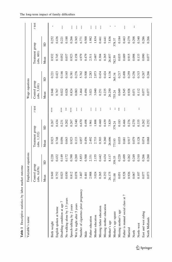
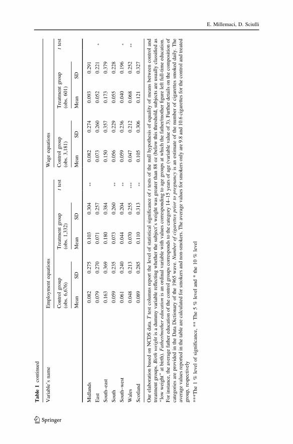
Table 1 contains descriptive statistics of the propensity score predictors distin-
guished by the total treatment indicator. Table 1 also reports the results of t tests of the
null hypothesis of equality of the means of the control group and the treatment groups.
The t test results reveal that the predictors of the probability of experiencing familial
problems at age seven often differ between the control and treatment groups, suggesting
that familial problems at age seven are not randomly distributed across groups.
In the employment equation, 1,332 individuals experience at least one family
difficulty. This means that the treated group is composed of 1,332 individuals when
the criterion is ‘‘having experienced at least one family difficulty’’ (Case A). Treated
individuals are also distinguished in terms of the number of family difficulties
experienced. Specifically, we isolate three sub-groups, identifying as specific
treatment groups (Case B): one family difficulty (63.4 % of cohort members), two
family difficulties (22.4 % of cohort members), or three or more family difficulties
(14.2 % of cohort members). Table 2 displays this information.6
To assess the effect of each specific family difficulty when it appears in association
with others, we isolate many treatment groups, separating single family difficulties
from multiple family difficulties. In the latter case, we associate each family difficulty
with one or more different family difficulties. This leaves us eighteen treatment groups,
5 On average, the balanced sample consists of approximately 15–18 % unemployed individuals,
12–15 % self-employed individuals and 70 % employed individuals.6 The percentage of cases for which a specific family difficulty appears as the only problem or associated
with other problems varies across family problem types. For example, about 60 % of housing problems at
age 7 are experienced as the only problem, while alcoholism appears as the only family problem at age 7
in just 5 % of cases. Further information about the distribution of family difficulties at age 7 across
specific family difficulties and their frequency of association is available upon request.
E. Millemaci, D. Sciulli
123
Ta
ble
1D
escr
ipti
ve
stat
isti
csb
yla
bor
mar
ket
ou
tco
me
Var
iab
le’s
nam
eE
mp
loy
men
teq
uat
ion
sW
age
equ
atio
ns
Con
tro
lg
rou
p
(ob
s.6
,676
)
Tre
atm
ent
gro
up
(ob
s.1
,33
2)
tte
stC
on
tro
lg
rou
p
(ob
s.3
,18
1)
Tre
atm
ent
gro
up
(ob
s.6
01
)
tte
st
Mea
nS
DM
ean
SD
Mea
nS
DM
ean
SD
Bir
thw
eig
ht
0.9
49
0.2
20
0.9
23
0.2
67
**
*0
.948
0.2
21
0.9
32
0.2
52
*
En
gli
shsp
oken
ath
om
e0
.752
0.4
32
0.7
48
0.4
34
0.7
67
0.4
23
0.7
45
0.4
36
Dis
abli
ng
con
dit
ion
atag
e7
0.0
23
0.1
49
0.0
56
0.2
31
**
*0
.022
0.1
46
0.0
52
0.2
21
***
No
wal
kin
gal
one
by
1.5
yea
rs0
.030
0.1
72
0.0
43
0.2
02
**
0.0
28
0.1
65
0.0
37
0.1
88
Sp
eech
-tal
kin
gb
y2
yea
rs0
.812
0.3
90
0.9
23
0.2
67
**
*0
.824
0.3
81
0.9
23
0.2
66
***
Wet
by
nig
ht
afte
r5
yea
rs0
.078
0.2
69
0.1
33
0.3
40
***
0.0
83
0.2
76
0.1
58
0.3
65
***
Num
ber
of
cigar
ette
spri
or
pre
gnan
cy3.4
87
5.8
53
4.8
57
6.6
70
***
3.4
64
5.7
62
4.9
79
6.7
71
***
Mal
e0
.481
0.5
00
0.4
56
0.4
98
0.4
94
0.5
00
0.4
79
0.5
00
Fat
her
edu
cati
on
2.9
88
2.3
31
2.4
92
1.9
61
***
3.0
21
2.2
83
2.5
11
1.9
82
***
Mo
ther
edu
cati
on
3.0
24
2.1
55
2.7
33
1.8
88
***
3.0
40
2.0
73
2.6
87
1.8
34
***
Mis
sing
fath
ered
uca
tion
0.2
65
0.4
42
0.3
03
0.4
60
***
0.2
51
0.4
34
0.3
04
0.4
61
***
Mis
sing
moth
ered
uca
tion
0.2
52
0.4
34
0.2
60
0.4
39
0.2
35
0.4
24
0.2
65
0.4
41
Mo
ther
’sag
e2
6.1
75
8.1
17
26
.69
67
.829
**
26
.25
08
.136
26
.85
77
.83
6*
Mo
ther
’sag
esq
uar
e7
51
.00
35
9.3
57
73
.93
37
9.2
4**
75
5.2
43
65
.34
78
2.5
93
78
.37
*
Mis
sin
gm
oth
er’s
age
0.0
51
0.2
20
0.0
35
0.1
83
**
0.0
49
0.2
17
0.0
35
0.1
84
Fat
her
ism
anu
also
cial
clas
sat
70
.528
0.4
99
0.6
81
0.4
66
***
0.5
45
0.4
98
0.6
89
0.4
63
***
Mar
ried
0.9
26
0.2
62
0.9
17
0.2
76
0.9
28
0.2
59
0.9
15
0.2
79
No
rth
0.0
67
0.2
49
0.0
79
0.2
70
0.0
71
0.2
56
0.0
98
0.2
98
**
No
rth
–w
est
0.1
07
0.3
10
0.1
28
0.3
35
**
0.1
12
0.3
15
0.1
33
0.3
40
Eas
tan
dw
est
rid
ing
0.0
77
0.2
66
0.0
74
0.2
62
0.0
77
0.2
67
0.0
90
0.2
86
No
rth
Mid
land
s0
.073
0.2
60
0.0
68
0.2
52
0.0
77
0.2
66
0.0
77
0.2
66
The long-term impact of family difficulties
123
Ta
ble
1co
nti
nu
ed
Var
iab
le’s
nam
eE
mp
loy
men
teq
uat
ion
sW
age
equ
atio
ns
Con
tro
lg
rou
p
(ob
s.6
,676
)
Tre
atm
ent
gro
up
(ob
s.1
,33
2)
tte
stC
on
tro
lg
rou
p
(ob
s.3
,18
1)
Tre
atm
ent
gro
up
(ob
s.6
01
)
tte
st
Mea
nS
DM
ean
SD
Mea
nS
DM
ean
SD
Mid
land
s0
.082
0.2
75
0.1
03
0.3
04
**
0.0
82
0.2
74
0.0
93
0.2
91
Eas
t0
.079
0.2
70
0.0
71
0.2
57
0.0
73
0.2
60
0.0
52
0.2
21
*
So
uth
–ea
st0
.163
0.3
69
0.1
80
0.3
84
0.1
50
0.3
57
0.1
73
0.3
79
So
uth
0.0
59
0.2
35
0.0
73
0.2
60
**
0.0
56
0.2
29
0.0
55
0.2
28
So
uth
–w
est
0.0
61
0.2
40
0.0
44
0.2
04
**
0.0
59
0.2
36
0.0
40
0.1
96
*
Wal
es0
.048
0.2
13
0.0
70
0.2
55
***
0.0
47
0.2
12
0.0
68
0.2
52
**
Sco
tlan
d0
.089
0.2
85
0.1
10
0.3
13
**
0.1
05
0.3
06
0.1
21
0.3
27
Ou
rel
abora
tion
bas
edo
nN
CD
Sd
ata.
Tte
stco
lum
ns
rep
ort
the
lev
elo
fst
atis
tica
lsi
gn
ifica
nce
of
tte
sts
of
the
nu
llh
yp
oth
esis
of
equ
alit
yo
fm
ean
sb
etw
een
con
tro
lan
d
trea
tmen
tg
rou
ps.
Bir
thw
eig
ht
isa
du
mm
yv
aria
ble
refl
ecti
ng
wh
ether
the
sub
ject
’sw
eig
ht
was
gre
ater
than
88
oz
(bel
ow
this
thre
sho
ld,
sub
ject
sar
eu
sual
lycl
assi
fied
as
‘‘lo
ww
eig
ht’’
atb
irth
).F
ath
er/m
oth
ered
uca
tio
nis
ano
rdin
alv
aria
ble
wit
hv
alues
corr
esp
on
din
gto
age
gro
ups
atw
hic
hth
efa
ther
/mo
ther
fig
ure
left
full
-tim
eed
uca
tio
n.
For
inst
ance
,th
eav
erag
efa
ther
educa
tion
of
the
contr
ol
gro
ups
corr
esponds
toth
eca
tegory
14–15
yea
rsof
age
(var
iable
val
ue
of
3).
Furt
her
det
ails
on
the
com
po
siti
on
of
cate
gori
esar
epro
vid
edin
the
Dat
aD
icti
onar
yof
the
1965
wav
e.N
um
ber
of
cig
aret
tes
pri
or
top
reg
nan
cyis
anes
tim
ate
of
the
num
ber
of
cigar
ette
ssm
oked
dai
ly.
The
aver
age
val
ues
rep
ort
edin
the
tab
lear
eca
lcu
late
dfo
rsm
ok
ers
and
no
n-s
mo
ker
s.T
he
aver
age
val
ues
for
smo
ker
so
nly
are
9.8
and
10
.6ci
gar
ette
sfo
rth
eco
ntr
ol
and
trea
ted
gro
up,
resp
ecti
vel
y
**
*T
he
1%
lev
elo
fsi
gn
ifica
nce
,*
*T
he
5%
lev
elan
d*
the
10
%le
vel
E. Millemaci, D. Sciulli
123
ten of which are effectively used in our econometric analysis. Similar considerations
are possible for the wage sample, but in the interest of brevity, these are not presented.
Table 3 displays the observed average employment probabilities and wages,
comparing treated and untreated individuals, when the criterion is ‘‘having experienced
at least one family difficulty’’. The results of t tests of the significance of the differentials
between the two groups are also reported. Both observed employment and wage
differentials remain quite constant over the period under investigation. Specifically, the
observed employment differential is approximately 5 % in 1991 and 2000 and
approximately 6 % in 2009, while the observed log-real wage differential is 0.09, 0.11
and 0.10, respectively, for the same years. In all cases, the differences are statistically
significant at the 1 % level.
3 Empirical model and estimation strategy
This section presents our estimation strategy for identifying the causal effect of
experiencing family difficulties at age seven on adult labor market outcomes.
Table 2 Number of family difficulties
No. of family
difficulties
Obs. Case A Case B Distribution by No. of
family difficulties (%)Group Obs. Group Obs.
0 6,676 Control 6,676 Control 6,676
1 845 Treatment 1332 First treatment 845 63.44
2 298 Second treatment 298 22.37
3 115 Third treatment 189 14.19
4 63
5 10
6 1
Our elaboration based on NCDS data
Table 3 Observed employment probabilities and wages
Group 1991 2000 2009
Mean SD Mean SD Mean SD
Employment
Control 0.818 0.386 0.879 0.326 0.871 0.335
Treatment 0.768 0.422 0.830 0.376 0.812 0.391
t test H0: l1 = l0 4.262 4.840 5.725
Log-real wages
Control 1.976 0.389 2.057 0.563 2.268 0.438
Treatment 1.885 0.368 1.944 0.523 2.169 0.414
t test H0: l1 = l0 5.293 4.555 5.133
Our elaboration based on NCDS data. Real wages are at 2009 constant values
The long-term impact of family difficulties
123
Because we are operating in a non-experimental setting, the estimation of the causal
effect of the treatment variable relies on the construction of a counterfactual using
the observational data of untreated cohort members. In fact, the selection bias
problem—which arises because of the non-random distribution of family difficulties
during childhood—may be econometrically addressed by applying matching
estimators (Caliendo and Kopeinig 2008). Matching estimators also have the
advantage that they do not require any assumption about the functional form of the
outcome equation, saving us from the risk of a misspecification bias (Todd 2008).
Given that we dispose of cross-sectional data, we make use of propensity score
matching (Rosenbaum and Rubin 1983). What we obtain is an estimate of the causal
effect as the average treatment effect on the treated (ATT). It follows that our casual
effect corresponds to the average difference between observed labor market outcomes
of cohort members experiencing (treated units) and not experiencing (untreated units)7
family difficulties at age seven, conditioned on the propensity score, i.e., on the
estimated probability of experiencing family difficulties at age seven. In fact,
according to the conditional mean independence assumption (CMIA), conditioning on
an adequate set of pre-treatment covariates is essential to remove all systematic
differences in outcomes in the untreated state and thereby address the selection bias
problem. We therefore estimate a logit model, controlling for an extensive set of
information contained in the NCDS about conditions and behaviors of the child and the
family, which can thus be considered good predictors of treatments and outcomes.
Because matching is only justified if performed over the common support region8
(Heckman et al. 1998), our estimations are based on observations of the treated
whose p scores are higher than the minimum or less than the maximum p score of
the untreated.
For the purpose of pairing treated and untreated units, we adopt two matching
methods (Becker and Ichino 2002): Gaussian kernel matching (GKM) and
Epanechnikov kernel matching (EKM).9 GKM and EKM can be considered
weighted regressions of the counterfactual outcome on an intercept with weights
given by the kernel weights.10 One major advantage of these approaches is the small
variance, which is achieved because more information is used, while a drawback is
that observations that are bad matches may also be used. To reduce this possible
source of bias, we restrict the bandwidth of the EKM to be quite tight (0.01).
7 Because we are studying the lasting impact of family difficulties at age seven from different
perspectives, treatment groups vary according to the specific aspect on which we are focusing.
Conversely, the control groups are constant across different perspectives and always consist of cohort
members who did not experience any family difficulty at age seven.8 The common support region is that for which the support of the covariates overlaps for the both
treatment and control groups.9 We also adopted a third matching method, namely, nearest neighbor matching (NNM). According to
the NNM method, an individual from the comparison group is chosen as a matching partner for a treated
individual who is closest in terms of propensity score. This method reduces the risk of comparing treated
individuals with untreated individuals who have too many different characteristics. On the other hand, the
variance is larger because less information is used, which reduces the significance of the estimated
parameters.10 The weights depend on the distance between each individual in the control group and the treated
observation for which the counterfactual is estimated (Smith and Todd 2005).
E. Millemaci, D. Sciulli
123
3.1 Assessing the validity of estimates beyond the CMIA
Although we are provided with a large and informative set of pre-treatment
variables, we cannot completely reject the possibility that unobservable factors
guide selection of our treatment variables, resulting in a violation of the CMIA.
To check whether and to what extent our results are sensitive to the failure of the
CMIA, we employ the sensitivity analysis proposed by Ichino et al. (2008). This
approach relies on the hypothesis that assignment to a treatment may be confounded,
given observable pre-treatment covariates, but that the confounding is removed once
we add an unobservable variable (U) to the observable pre-treatment covariates. On
the basis of this method, we estimate new ATTs and compare them with baseline
ATTs, estimated under the CMIA, to reveal the extent of their hypothetical deviations.
Following Ichino et al. (2008), we simulate the distribution of alternative unobserv-
able terms, imposing the condition that they are similar to the empirical distribution of
some relevant binary observable covariates. Specifically, we identify the simulated
distribution by means of four sensitivity parameters (p11, p10, p01, p00), where
parameter pij is the probability that the unobserved factor takes the value 1 for an
individual with treatment status i and outcome status j.11
A further robustness analysis is carried out, relaxing the assumption that the
distribution of unobservable factors, given the treatment variable and the outcomes,
completely replicates the distribution of observable variables. We allow the sensitivity
parameters to shift from their starting values by d = |p01 - p00| and s = |p1. - p0.|,
and we consider four cases, d [ 0 and s [ 0, d \ 0 and s \ 0, d [ 0 and s \ 0, d \ 0
and s [ 0, where d and s take, in turn, the values 0.1, 0.2, 0.3 and 0.4. We provide
further information concerning the outcome and the selection effects that correspond,
in turn, to the association between unobservable factors and the outcome of untreated
units and the association between unobservable factors and the treatment variable. As
we explain in Sect. 4.1 (commenting on simulation results), these two indicators are
useful in assessing the plausibility of simulated estimates of ATTs.
4 Estimation results
Our estimation results obtained using the GKM and EKM techniques12 are reported
in Tables 4, 5, 6 and 7.13 As mentioned above, we consider two different types of
labor market outcomes: employment status and employees’ logs of hourly wages.
11 In case the outcome is continuous, we consider a binary transformation of the outcome.12 The balancing property of propensity scores is checked using the STATA’s command ‘‘pscore’’
employed by Becker and Ichino (2002). PSM estimations are obtained by means of two other commands
(‘‘attk’’ and ‘‘attnd’’) employed by the same authors, set at default parameters but with a bandwidth of
0.01 in the case of EKM, and with the options ‘‘logit’’ and ‘‘comsup’’. The latter is enabled so that ATT
estimations only use observations inside the common support. Standard errors are computed using the
bootstrap technique with replications set at 500.13 We also use standard econometric techniques (probit and ordinary least squares models) to estimate
the effects of family difficulties on adult labor market outcomes. The results are consistent with those
obtained using matching methods and are available upon request.
The long-term impact of family difficulties
123
The treatments under examination are whether at least one, exactly one, exactly
two, or at least three family difficulties were experienced. Other treatments are
whether housing, economic, physical, mental, and disharmony problems were
individually experienced as the only family difficulty or in association with others.
Examining the support condition with propensity scores of the treated and
untreated groups of subjects in specific figures, it emerges that in all cases the
overlapped region is wide. The number of observations removed because of not
satisfying the common support condition never exceeds 16 %. Moreover, using the
STATA’s command ‘‘pstest’’ employed by Leuven and Sianesi (2003), we run
propensity balancing tests (Rosenbaum and Rubin 1985) for equality of the means
of the control variables in the treated and untreated groups both before and after
matching. The results show that the matching procedure significantly reduces the
bias between the treated and untreated groups. Overall, after matching, none of the
control variables are significantly different between the groups.14
For each treatment and subject age considered (33, 42 and 51 years old), we
report the estimated average treatment effects of the treated individuals (ATT),
bootstrapped standard errors, t statistics and the number of treated and control
individuals used with each matching technique.
As anticipated, the causal effect we estimate corresponds to the total effect—the
sum of the direct and indirect effects.15 We expect the direct effect of a treatment to
have a negative impact on labor market outcomes. With regard to the indirect
effects, on the one hand, we expect that family problems may reduce the
accumulation of human capital. On the other hand, these problems may trigger
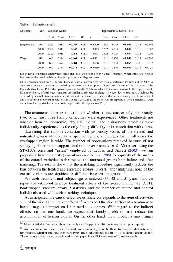
Table 4 Estimation results
Outcomes Years Gaussian Kernel Epanechnikov Kernel (0.01)
Labor market outcomes: employment status and log of employee’s hourly wage. Treatment: Whether the family has at
least one of the listed problems. Propensity score matching estimates
Our elaboration based on NCDS data. Propensity score matching estimations are performed by means of the STATA
commands attk and attnd, using default parameters and the options ‘‘logit’’ and ‘‘comsup’’. In the case of the
Epanechnikov kernel PSM, the options epan and bwidth (0.01) are added to the attk command. The reported coef-
ficients of the log of real wage equations are similar to the percent change in wages due to treatment, which can be
obtained by a simple transformation: exp(treatment coefficient) 2 1. Values that are statistically significant at the 1
and 5 % levels are reported in bold; values that are significant at the 10 % level are reported in bold and italics. T-stats
are obtained using standard errors bootstrapped with 500 replications (SE)
14 More detailed information about the analysis of support conditions is available upon request.15 Another important issue is to understand how disadvantages in childhood transmit to adult outcomes:
for instance, whether and how they negatively affect educational, health or social capital accumulation.
These latter aspects are not considered in this paper but will be subjects of future research.
E. Millemaci, D. Sciulli
123
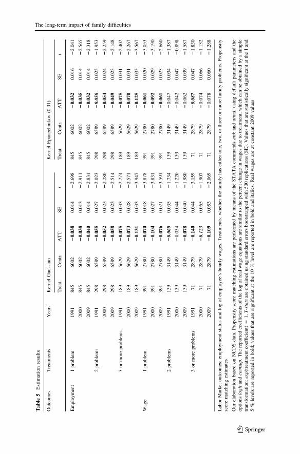
Ta
ble
5E
stim
atio
nre
sult
s
Outc
om
esT
reat
men
tsY
ears
Ker
nel
Gau
ssia
nK
ernel
Epan
echnik
ov
(0.0
1)
Tre
at.
Contr
.A
TT
SE
tT
reat
.C
ontr
.A
TT
SE
t
Em
plo
ym
ent
1pro
ble
m1991
845
6002
20.0
38
0.0
14
22.6
98
845
6002
20.0
32
0.0
16
22.0
41
2000
845
6002
20.0
38
0.0
13
22.9
11
845
6002
20.0
35
0.0
14
22.5
65
2009
845
6002
20.0
40
0.0
14
22.8
31
845
6002
20.0
32
0.0
14
22.3
18
2pro
ble
ms
1991
298
6589
20.0
55
0.0
27
22.0
23
298
6589
20.0
50
0.0
25
21.9
53
2000
298
6589
20.0
52
0.0
23
22.2
80
298
6589
20.0
54
0.0
24
22.2
59
2009
298
6589
20.0
58
0.0
23
22.5
14
298
6589
20.0
49
0.0
23
22.1
48
3or
more
pro
ble
ms
1991
189
5629
20.0
75
0.0
33
22.2
74
189
5629
20.0
75
0.0
31
22.4
02
2000
189
5629
20.0
73
0.0
28
22.5
71
189
5629
20.0
70
0.0
31
22.2
67
2009
189
5629
20.1
31
0.0
33
23.9
47
189
5629
20.1
25
0.0
35
23.5
67
Wag
e1
pro
ble
m1991
391
2780
20.0
70
0.0
18
23.8
78
391
2780
20.0
61
0.0
20
23.0
53
2000
391
2780
20.1
04
0.0
27
23.8
31
391
2780
20.0
92
0.0
29
23.1
90
2009
391
2780
20.0
76
0.0
21
23.5
91
391
2780
20.0
61
0.0
23
22.6
60
2pro
ble
ms
1991
139
3149
20.0
60
0.0
35
21.7
34
139
3149
20.0
47
0.0
34
21.3
87
2000
139
3149
20.0
54
0.0
44
21.2
20
139
3149
20.0
42
0.0
47
20.8
98
2009
139
3149
20.0
78
0.0
40
21.9
80
139
3149
20.0
62
0.0
39
21.5
87
3or
more
pro
ble
ms
1991
71
2879
20.1
40
0.0
44
23.1
59
71
2879
20.0
87
0.0
47
21.8
30
2000
71
2879
20.1
23
0.0
65
21.9
07
71
2879
20.0
74
0.0
66
21.1
32
2009
71
2879
20.1
09
0.0
53
22.0
69
71
2879
20.0
78
0.0
60
21.2
88
Lab
or
Mar
ket
outc
om
es:
emplo
ym
ent
stat
us
and
log
of
emplo
yee
’shourl
yw
ages
.T
reat
men
ts:
whet
her
the
fam
ily
has
eith
erone,
two,
or
thre
eor
more
fam
ily
pro
ble
ms.
Pro
pen
sity
score
mat
chin
ges
tim
ates
Our
elab
ora
tion
bas
edon
NC
DS
dat
a.P
ropen
sity
score
mat
chin
ges
tim
atio
ns
are
per
form
edby
mea
ns
of
the
ST
AT
Aco
mm
ands
att
kan
datt
nd
,usi
ng
def
ault
par
amet
ers
and
the
opti
ons
logit
and
com
sup
.T
he
report
edco
effi
cien
tsof
the
log
of
real
wag
eeq
uat
ions
are
sim
ilar
toth
eper
cent
chan
ge
inw
ages
due
totr
eatm
ent,
whic
hca
nbe
obta
ined
by
asi
mple
tran
sform
atio
n:
exp
(tre
atm
ent
coef
fici
ent)
21.
T-s
tats
are
obta
ined
usi
ng
stan
dar
der
rors
boots
trap
ped
wit
h500
repli
cati
ons
(SE
).V
alues
that
are
stat
isti
call
ysi
gnifi
cant
atth
e1
and
5%
level
sar
ere
port
edin
bold
;val
ues
that
are
signifi
cant
atth
e10
%le
vel
are
report
edin
bold
and
ital
ics.
Rea
lw
ages
are
atco
nst
ant
2009
val
ues
The long-term impact of family difficulties
123
Ta
ble
6S
pec
ific
fam
ily
dif
ficu
ltie
s
Gau
ssia
nK
ernel
PS
MO
nly
one
pro
ble
mA
pro
ble
mas
soci
ated
wit
hoth
ers
Tre
at.
Co
ntr
.A
TT
SE
tT
reat
.C
on
tr.
AT
TS
Et
Ho
usi
ng
19
91
24
06
51
82
0.0
560
.027
22
.086
17
65
40
02
0.0
86
0.0
34
22
.497
20
00
24
06
51
82
0.0
480
.024
22
.002
17
65
40
02
0.0
54
0.0
31
21
.749
20
09
24
06
51
82
0.0
18
0.0
24
20
.734
17
65
40
02
0.1
00
0.0
32
23
.152
Eco
no
mic
19
91
12
35
66
72
0.1
01
0.0
39
20
.734
30
86
61
72
0.0
87
0.0
25
23
.502
20
00
12
35
66
72
0.0
49
0.0
34
21
.446
30
86
61
72
0.0
78
0.0
24
23
.274
20
09
12
35
66
72
0.1
360
.043
23
.138
30
86
61
72
0.1
24
0.0
26
24
.792
Ph
ysi
cal
19
91
11
46
62
40
.008
0.0
35
0.2
44
14
15
21
12
0.1
06
0.0
37
22
.832
20
00
11
46
62
42
0.0
43
0.0
34
21
.266
14
15
21
12
0.0
47
0.0
33
21
.447
20
09
11
46
62
40
.027
0.0
28
0.9
60
14
15
21
12
0.1
09
0.0
37
22
.953
Men
tal
19
91
79
53
83
20
.012
0.0
43
20
.282
13
35
31
12
0.0
71
0.0
38
21
.885
20
00
79
53
83
20
.047
0.0
41
21
.165
13
35
31
12
0.0
87
0.0
35
22
.485
20
09
79
53
83
20
.027
0.0
42
20
.625
13
35
31
12
0.0
86
0.0
35
22
.452
Dis
har
mo
ny
19
91
14
46
53
42
0.0
27
0.0
33
20
.808
26
46
56
82
0.0
30
.026
21
.178
20
00
14
46
53
42
0.0
51
0.0
32
21
.588
26
46
56
82
0.0
67
0.0
27
22
.486
20
09
14
46
53
42
0.0
54
0.0
33
21
.625
26
46
56
82
0.0
87
0.0
26
23
.404
Em
plo
ym
ent
stat
us.
Gau
ssia
nK
ern
elP
ropen
sity
Sco
reM
atch
ing
Ou
rel
abora
tio
nb
ased
on
NC
DS
dat
a.P
ropen
sity
sco
rem
atch
ing
esti
mat
ion
sar
ep
erfo
rmed
by
mea
ns
of
the
ST
AT
Aco
mm
and
att
ku
sin
gd
efau
ltp
aram
eter
san
do
pti
on
s
‘‘lo
git
’’,
‘‘co
msu
p’’.
Sta
tist
ical
lysi
gn
ifica
nt
resu
lts
atth
e1
and
5%
lev
els
are
rep
ort
edin
bo
ld;
sign
ifica
nt
val
ues
atth
e1
0%
lev
elar
ein
bo
ldan
dit
alic
.T
-sta
tsar
e
obta
ined
by
usi
ng
stan
dar
der
rors
boots
trap
ped
wit
h500
repli
cati
ons
(SE
)
E. Millemaci, D. Sciulli
123
Ta
ble
7S
pec
ific
fam
ily
dif
ficu
ltie
s
Gau
ssia
nK
ernel
PS
MO
nly
one
pro
ble
mA
pro
ble
mas
soci
ated
wit
hoth
ers
Tre
at.
Co
ntr
.A
TT
SE
tT
reat
.C
on
tr.
AT
TS
Et
Ho
usi
ng
19
91
11
82
67
82
0.0
80
.033
22
.572
71
24
16
20
.11
0.0
48
22
.214
20
00
11
82
67
82
0.1
50
.045
23
.355
71
24
16
20
.14
0.0
67
22
.095
20
09
11
82
67
82
0.1
0.0
42
2.5
77
71
24
16
20
.08
10
.052
21
.57
Eco
no
mic
19
91
52
25
92
20
.10
.043
22
.357
12
82
88
12
0.1
0.0
32
3.4
32
20
00
52
25
92
20
.12
0.0
72
1.7
49
12
82
88
12
0.1
0.0
46
22
.223
20
09
52
25
92
20
.10
.05
22
.063
12
82
88
12
0.1
30
.038
23
.45
Ph
ysi
cal
19
91
51
25
14
20
.071
0.0
59
21
.192
60
24
56
20
.11
0.0
52
22
.002
20
00
51
25
14
0.0
04
0.0
62
0.0
65
60
24
56
20
.05
00
.066
20
.756
20
09
51
25
14
20
.082
0.0
59
21
.392
60
24
56
20
.03
60
.058
20
.61
Men
tal
19
91
32
24
12
20
.089
0.0
52
21
.735
60
23
58
20
.10
30
.056
21
.849
20
00
32
24
12
20
.156
0.1
46
21
.068
60
23
58
20
.03
60
.074
20
.492
20
09
32
24
12
20
.10
.075
21
.343
60
23
58
20
.07
00
.06
21
.16
Dis
har
mo
ny
19
91
68
31
25
20
.067
0.0
42
21
.61
10
30
96
20
.05
20
.04
21
.295
20
00
68
31
25
20
.065
0.0
58
21
.115
11
03
09
60
.01
60
.051
0.3
09
20
09
68
31
25
20
.027
0.0
51
20
.534
11
03
09
62
0.0
59
0.0
42
21
.405
Ou
tcom
e:L
og
of
ho
url
yw
age.
Gau
ssia
nk
ern
elp
rop
ensi
tysc
ore
mat
chin
g
Ou
rel
abora
tio
nb
ased
on
NC
DS
dat
a.P
ropen
sity
sco
rem
atch
ing
esti
mat
ion
sar
ep
erfo
rmed
by
mea
ns
of
the
ST
AT
Aco
mm
and
att
k,u
sin
gd
efau
ltp
aram
eter
san
dth
e
op
tio
ns
log
itan
dco
msu
p.T
he
rep
ort
edco
effi
cien
tso
fth
elo
go
fre
alw
age
equ
atio
ns
are
sim
ilar
toth
ep
erce
nt
chan
ge
inw
ages
du
eto
trea
tmen
t,w
hic
hca
nb
eo
bta
ined
by
asi
mple
tran
sform
atio
n:
exp(
trea
tmen
tco
effi
cien
t)2
1.
T-s
tats
are
ob
tain
edu
sin
gst
and
ard
erro
rsb
oo
tstr
app
edw
ith
50
0re
pli
cati
on
s(S
E).
Val
ues
that
are
stat
isti
call
y
sig
nifi
can
tat
the
1an
d5
%le
vel
sar
ere
po
rted
inb
old
;v
alu
esth
atar
esi
gn
ifica
nt
atth
e1
0%
lev
elar
ere
po
rted
inb
old
and
ital
ics.
Rea
lw
ages
are
atco
nst
ant
20
09
lev
els
The long-term impact of family difficulties
123
children’s efforts and determination at school and make them achieve better and/or
quicker outcomes in the labor market. However, our view is that the net average
indirect effect is negative, as is the direct one. Thus, we expect the total effect to be
negative, but we are not able to make predictions about the mid- and long-term
intensities of such effects.
For comparative purposes across time, most of our analysis is restricted to
children for whom information is not missing and who participated in all five
sweeps. The consequent attrition and item non-response reduce the amount of
usable information. However, as noted by Dearden et al. (1997), attrition and non-
response are more likely to be associated with individuals with lower abilities and
lower educational attainments. Because it is likely that among individuals with
family difficulties, those who obtain poorer labor market outcomes are those who
perform more poorly in school, we consider our estimates conservative.
From our estimations, we find that the estimated ATT for the treatment that
corresponds to experiencing at least one family difficulty in childhood (Table 4) is
always statistically significant at the 1 % level, with both kernel matching
estimators having significant parameters, ranging between -0.039 and -0.054 for
the employment status outcome and between 0.056 and 0.084 for the log of hourly
wages outcome.16
Turning to the treatments corresponding to whether the subject had (1) only one
family problem or (2) two or (3) three or more (Table 5), we observe that the ATT
coefficients are almost always significant at conventional levels and have values that
increase with the number of problems: (1) (-0.032/-0.04), (2) (-0.049/-0.058)
and (3) (-0.07/-0.131) for employment status. This evidence confirms the
expectation that an increase in family problems has more serious effects on adult
labor market outcomes. Considering the wage outcomes, we note that our sample
consists of a few individuals with two or more problems. For this reason, the
variances are larger, and even in the presence of similar ATTs, the results are
sometimes statistically insignificant. Nonetheless, the increasing trend seems to be
confirmed.
The results shown in Tables 4 and 5 suggest that family difficulties have long-
term lasting effects that do not tend to disappear even after more than forty years.
Moreover, the estimated ATTs do not exhibit any declining trends over the two
decades of observation (1991–2009).
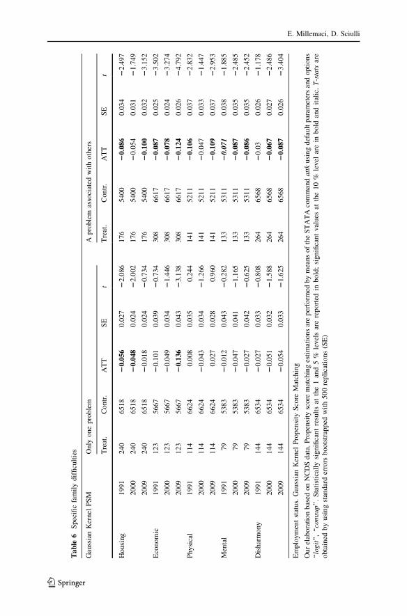
When we consider specific family difficulties, we distinguish between (I) the case
in which the problem is the only one attributed to the family or (II) the problem is
associated with one or more additional problems. For case (I), we find evidence of
statistically significant negative effects of housing and economic family problems in
childhood on adult employment status (Table 6).17 This agrees with findings
reported in the literature (e.g., Gregg and Machin 2000), even though our estimates
16 The reported coefficients of the log of real wage equations are similar to the percent change in wages
due to the treatment and can be obtained by a simple transformation: exp(treatment coefficient) - 1.
Therefore, the corresponding average wage reduction falls in the range between 5.5 and 8.1%.17 Only the results obtained using Gaussian kernel propensity score matching are reported in Table 6
because the results (available upon request) obtained using the Epanechnikov kernel matching technique
did not differ significantly.
E. Millemaci, D. Sciulli
123
are slightly smaller in magnitude than the results reported in studies conducted using
standard econometric techniques. However, it is interesting to note that the results
are substantially different when we consider case (II). Not only housing and
economic difficulties but also physical, mental and disharmony difficulties are
frequently significant. In all cases but that of economic distress, we notice that the
parameter values are larger and the standard errors are smaller for case (II) than for
(I), resulting in higher t statistics. This finding suggests that if housing and economic
problems in a family have long-term negative consequences on children, physical,
mental and disharmony family problems produce serious negative effects only when
the family also experiences other problems. This result may be explained in terms of
a cumulative effect and/or in terms of an association effect. On the one hand, the
cumulative effect indicates that physical, mental or familial disharmony problems
during childhood do not reduce adult labor market potential per se but that they do
have a negative impact if accompanied by other problems. While a family can
effectively handle one problem without future negative consequences for children’s
labor market outcomes, it may not succeed in doing so when numerous problems
occur simultaneously. On the other hand, the association effect suggests that the
negative effects of physical, mental or familial disharmony problems may be due to
other problems (e.g., housing and economic difficulties) that are possibly the latent
causes of poor adult labor market outcomes.18 It follows that our results agree with
those that question a genuine negative effect of family disharmony (e.g., divorce) on
later outcomes (e.g., Sanz de Galdeano and Vuri 2007), albeit from a different
perspective.
It is also interesting to note that, in line with the results of previous studies,
family disharmony does not seem to have a homogeneous effect on labor outcomes
for males and females. In particular, when we estimate ATTs for the two groups
separately, we find some evidence that the effect is more negative for men than for
women, which is consistent with the findings reported by Corak (2001).
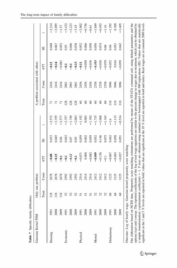
With regard to the wage outcome, we find that housing and economic problems
have even more intense and significant negative effects in terms of percentages. We
cannot reject the hypothesis that other family problems in childhood do not have an
impact on wages in adulthood. Moreover, comparing the results of cases (I) and (II),
we observe that the significant parameters are similar for all of the specific problems
(Table 7).
The decision to restrict the sample to individuals whose complete information is
available for all three adulthood waves of year 1991, 2000 and 2009 implies an
important reduction in the dimension of the sample and makes it difficult to
efficiently estimate the effect on labor market outcomes of each specific family
problem. To understand how this source of selection affects the results, we compute
18 Given the partially non-mutually exclusive nature of different types of treatments, our approach to
assessing the effect of each specific problem was to calculate the ATTs for the case of individuals with
one problem and concurrent problems. As underlined by one referee, it should be specified that the ATT
for ‘‘only one problem’’ may not approximate the marginal impact of that particular problem (because
individuals with only problem ‘‘x’’ are a subset of all individuals with problem ‘‘x’’).
The long-term impact of family difficulties
123
ATTs using all individuals with complete information on outcomes and matching
variables for the wave of year 2009 and employed the GKM technique.19
For the employment equation, we obtain more negative (by approximately 30 %)
and always statistically significant values of the ATTs when we consider family
difficulties as a whole. In the case of specific problems, the estimated ATTs are all
more negative and always statistically significant when they appear associated with
other problems. When we consider specific problems as the only family difficulty
experienced by an individual, only economic and family disharmony problems have
a significant negative impact (at conventional levels) on employment for the larger
sample. For the wage equation, the new estimated ATTs are always more negative
than those estimated using the smaller sample (by 25–30 %, on average) and are
all20 statistically significant for family difficulties considered as a whole and for
specific types of difficulties.
This evidence suggests that individuals excluded by our samples are likely to fill
the weakest positions in the labor market: for example, they are likely to experience
greater turnover and therefore accumulate less job experience. Therefore, the
estimates presented in this paper can be considered conservative.
4.1 Sensitivity analysis
As mentioned above, the reliability of the previous PSM estimates depends on the
plausibility of the CMIA, which is not testable. The large set of variables we include
in the matching model as covariates allows us to be confident that we are controlling
for the most relevant confounders. Moreover, we employ a simulation-based
sensitivity analysis to assess the reliability of the estimated results with respect to
hypothetical failures of the CMIA.
Estimates from simulation-based sensitivity analyses are obtained using the
STATA routine ‘‘sensatt’’, implemented by Nannicini (2007). The estimates are
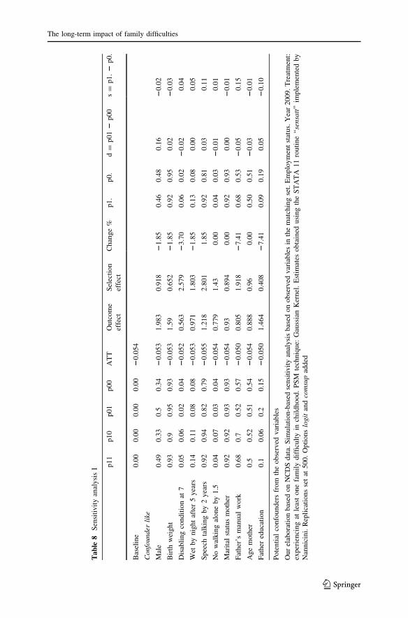
reported in Tables 8 and 9.21 In the interest of brevity, we present only the
sensitivity analysis for the case where the treated observations are those that
involved at least one family difficulty at the age of seven and the controls are those
with no reported difficulties. Moreover, we concentrate on the outcome of
employment status and the year 2009. The PSM technique adopted is the Gaussian
kernel technique.
19 The samples for the employment and wage equations now consist of 9,762 and 6,238 observations,
respectively. Tables with results of these estimates are not reported for the sake of brevity but are
available upon request.20 In the case of family disharmony as the only difficulty, the ATT is not statistically significant, while it
becomes significant at the 1% level (with a parameter value of 0.127) when associated with other family
difficulties. This result is consistent with evidence reported for the case of the employment equation with
the smaller sample.21 The ‘‘sensatt’’ routine simulates a binary confounder with parameters defined based on the two
alternative approaches described in the text. The simulated confounder is then treated as an additional
regressor in the estimation of the propensity score and in the subsequent computation of the ATT. The
procedure is repeated for a large number of simulations of the confounder (which we set at 500), and the
final ATT is calculated as the average of the individual ATTs across all the simulations. The standard
error is computed as the average variance of the ATT across all the simulations.
E. Millemaci, D. Sciulli
123
Ta
ble
8S
ensi
tiv
ity
anal
ysi
sI p
11
p1
0p
01
p0
0A
TT
Ou
tcom
e
effe
ct
Sel
ecti
on
effe
ct
Ch
ang
e%
p1
.p
0.
d=
p0
12
p0
0s
=p
1.
2p
0.
Bas
elin
e0
.00
0.0
00
.00
0.0
02
0.0
54
Con
fou
nde
rli
ke
Mal
e0
.49
0.3
30
.50
.34
20
.05
31
.983
0.9
18
21
.85
0.4
60
.48
0.1
62
0.0
2
Bir
thw
eig
ht
0.9
30
.90
.95
0.9
32
0.0
53
1.5
90
.652
21
.85
0.9
20
.95
0.0
22
0.0
3
Dis
abli
ng
con
dit
ion
at7
0.0
50
.06
0.0
20
.04
20
.05
20
.563
2.5
79
23
.70
0.0
60
.02
20
.02
0.0
4
Wet
by
nig
ht
afte
r5
yea
rs0
.14
0.1
10
.08
0.0
82
0.0
53
0.9
71
1.8
03
21
.85
0.1
30
.08
0.0
00
.05
Sp
eech
talk
ing
by
2y
ears
0.9
20
.94
0.8
20
.79
20
.05
51
.218
2.8
01
1.8
50
.92
0.8
10
.03
0.1
1
No
wal
kin
gal
one
by
1.5
0.0
40
.07
0.0
30
.04
20
.05
40
.779
1.4
30
.00
0.0
40
.03
20
.01
0.0
1
Mar
ital
stat
us
moth
er0
.92
0.9
20
.93
0.9
32
0.0
54
0.9
30
.894
0.0
00
.92
0.9
30
.00
20
.01
Fat
her
’sm
anu
alw
ork
0.6
80
.70
.52
0.5
72
0.0
50
0.8
05
1.9
18
27
.41
0.6
80
.53
20
.05
0.1
5
Ag
em
oth
er0
.50
.52
0.5
10
.54
20
.05
40
.888
0.9
60
.00
0.5
00
.51
20
.03
20
.01
Fat
her
edu
cati
on
0.1
0.0
60
.20
.15
20
.05
01
.464
0.4
08
27
.41
0.0
90
.19
0.0
52
0.1
0
Po
ten
tial
con
fou
nd
ers
fro
mth
eo
bse
rved
var
iab
les
Ou
rel
abora
tion
bas
edo
nN
CD
Sd
ata.
Sim
ula
tion
-bas
edse
nsi
tiv
ity
anal
ysi
sb
ased
on
ob
serv
edv
aria
ble
sin
the
mat
chin
gse
t.E
mp
loy
men
tst
atu
s.Y
ear
20
09
.T
reat
men
t:
exp
erie
nci
ng
atle
ast
on
efa
mil
yd
iffi
cult
yin
chil
dh
oo
d.
PS
Mte
chniq
ue:
Gau
ssia
nK
ern
el.
Est
imat
eso
bta
ined
usi
ng
the
ST
AT
A1
1ro
uti
ne
‘‘se
nsa
tt’’
imp
lem
ente
db
y
Nan
nic
ini.
Rep
lica
tions
set
at500.
Opti
ons
logi
tan
dco
msu
pad
ded
The long-term impact of family difficulties
123
Ta
ble
9S
ensi
tiv
ity
anal
ysi
sII
AT
TS
EO
ut.
Eff
.S
el.
Eff
.A
TT
SE
Out.
Eff
.S
el.
Eff
.A
TT
SE
Out.
Eff
.S
el.
Eff
.A
TT
SE
Out.
Eff
.S
el.
Eff
.
s=
0.1
s=
0.2
s=
0.3
s=
0.4
1)
d[
0an
ds[
0
d=
0.1
20.0
56
0.0
01
1.4
87
1.4
91
20.0
59
0.0
02
1.5
09
2.2
57
20.0
63
0.0
03
1.4
93.5
83
20.0
70.0
04
1.5
27.1
42
d=
0.2
20.0
59
0.0
01
2.4
32
1.5
17
20.0
66
0.0
02
2.4
22.2
78
20.0
76
0.0
03
2.4
27
3.6
28
20.0
87
0.0
04
2.4
53
6.5
01
d=
0.3
20.0
63
0.0
02
4.6
43
1.5
34
20.0
74
0.0
02
4.6
17
2.3
11
20.0
89
0.0
03
4.6
3.6
38
20.1
06
0.0
04
4.6
23
6.3
59
d=
0.4
20.0
65
0.0
02
15.5
46
1.5
20.0
80.0
03
15.5
73
2.2
59
20.1
01
0.0
03
15.7
82
3.4
99
20.1
24
0.0
03
15.8
28
5.9
6
AT
TS
EO
ut.
Eff
.S
el.
Eff
.A
TT
SE
Out.
Eff
.S
el.
Eff
.A
TT
SE
Out.
Eff
.S
el.
Eff
.A
TT
SE
Out.
Eff
.S
el.
Eff
.
s=
-0.1
s=
-0.2
s=
-0.3
s=
-0.4
2)
d\
0an
ds\
0
d=
-0.1
20.0
59
0.0
01
0.2
99
0.5
03
20.0
68
0.0
02
0.2
98
0.3
05
20.0
80.0
03
0.2
99
0.2
20.0
91
0.0
04
0.2
99
0.1
33
d=
-0.2
20.0
61
0.0
01
0.1
57
0.6
09
20.0
71
0.0
02
0.1
57
0.3
97
20.0
86
0.0
03
0.1
59
0.2
63
20.1
02
0.0
03
0.1
58
0.1
74
d=
-0.3
20.0
64
0.0
02
0.0
97
0.6
44
20.0
76
0.0
02
0.0
97
0.4
28
20.0
94
0.0
03
0.0
96
0.2
83
20.1
13
0.0
03
0.0
98
0.1
81
d=
-0.4
20.0
66
0.0
02
0.0
64
0.6
54
20.0
82
0.0
03
0.0
64
0.4
36
20.1
03
0.0
03
0.0
65
0.2
77
20.1
26
0.0
03
0.0
64
0.1
61
3)
d[
0an
ds\
0
d=
0.1
20.0
48
0.0
01
1.8
97
0.5
59
20.0
39
0.0
03
1.9
18
0.3
47
20.0
30.0
04
1.9
06
0.2
29
20.0
21
0.0
06
1.8
96
0.1
53
d=
0.2
20.0
43
0.0
02
3.0
83
0.5
53
20.0
27
0.0
04
3.0
90.3
51
20.0
10.0
05
3.0
85
0.2
32
20.0
21
0.0
06
1.8
96
0.1
52
d=
0.3
20.0
39
0.0
03
4.7
45
0.5
77
20.0
19
0.0
04
4.6
97
0.3
68
0.0
03
0.0
05
4.6
71
0.2
55
0.0
32
0.0
07
4.6
83
0.1
62
d=
0.4
20.0
37
0.0
03
7.0
59
0.5
99
20.0
11
0.0
05
6.9
83
0.3
83
0.0
21
0.0
06
7.0
49
0.2
54
0.0
52
0.0
07
7.0
29
0.1
7
E. Millemaci, D. Sciulli
123
Ta
ble
9co
nti
nu
ed
AT
TS
EO
ut.
Eff
.S
el.
Eff
.A
TT
SE
Out.
Eff
.S
el.
Eff
.A
TT
SE
Out.
Eff
.S
el.
Eff
.A
TT
SE
Out.
Eff
.S
el.
Eff
.
s=
0.1
s=
0.2
s=
0.3
s=
0.4
4)
d\
0an
ds[
0
d=
20.1
20.0
49
0.0
01
0.5
29
1.9
16
20.0
42
0.0
02
0.5
37.5
85
20.0
40.0
03
0.6
64.8
39
20.0
35
0.0
04
0.6
69
7.2
23
d=
20.2
20.0
42
0.0
02
0.5
37.5
85
20.0
42
0.0
02
0.5
37.5
85
20.0
22
0.0
03
0.3
25
24.2
32
20.0
17
0.0
03
0.4
41
8.1
53
d=
20.3
20.0
44
0.0
02
0.2
15
1.5
43
20.0
30.0
02
0.2
14
2.6
26
20.0
14
0.0
03
0.2
15
5.6
35
0.0
01
0.0
03
0.2
72
8.5
01
d=
20.4
20.0
42
0.0
02
0.1
43
1.4
79
20.0
25
0.0
03
0.1
44
2.3
04
20.0
01
0.0
03
0.0
64
5.9
71
0.0
16
0.0
04
0.1
44
8.9
78
Pote
nti
alco
nfo
under
sby
incr
easi
ng
abso
lute
val
ues
of
dan
ds
Our
elab
ora
tion
bas
edon
NC
DS
dat
a.S
imula
tion-b
ased
sensi
tivit
yan
alysi
sbas
edon
com
bin
atio
ns
of
incr
easi
ng
abso
lute
val
ues
of
dan
ds.
Em
plo
ym
ent
stat
us.
Yea
r2009.
Tre
atm
ent:
exper
ienci
ng
atle
ast
one
fam
ily
dif
ficu
lty
inch
ildhood.
PS
Mte
chniq
ue:
Gau
ssia
nker
nel
.E
stim
ates
obta
ined
usi
ng
the
ST
AT
A11
routi
ne
‘‘se
nsa
tt’’
imple
men
ted
by
Nan
nic
ini.
Rep
lica
tions
set
at500.
Opti
ons
logit
and
com
sup
added
The long-term impact of family difficulties
123
Table 8 reports the results for the confounding factor U calibrated to mimic
different observable variables included in the matching set. The baseline ATT
estimate (-0.054) represents the value obtained with no confounder in the matching
set. On the subsequent row, the confounder is hypothesized to have the same pijvalues as those of the gender variable. Given that 49 % of the subjects who
experienced at least one family problem and are employed are male, by setting
p11 = 0.49, we are imposing the constraint that an identical fraction of subjects have
a value of U equal to 1. An analogous interpretation holds for the other probabilities
pij in the row. In this case, the unobserved factor has a positive effect on the relative
probability of getting a job (outcome effect = 1.983 [ 1), has no effect on the
relative probability of being treated (selection effect = 0.918 & 1), and produces a
very small change in ATT (-0.053). Similarly, we proceed in the other rows,
choosing parameters pij to equal those of the other binary variables22 of the matching
set: birth weight, disability at age seven, bed-wetting after 5 years, talking by
2 years, not walking by 1.5 years, marital status of the mother, whether the father is
employed in manual work, the age of the mother, and the father’s education. We find
that the baseline ATT estimate is very stable because the simulated ATTs are very
similar and never predict parameter values that diverge by more than 7.4 %.
Moreover, these simulations show that both the outcome and the selection effect of
U must be strong to represent a threat to the significance of the estimated ATT.
Table 9 shows results with pij imposed such that all combinations of d and s (up to
0.4 in absolute terms) are considered. This exercise allows us to explore the
characteristics of the confounding factor that make the ATT decrease to zero. As
discussed above, increasing values of d and s correspond to more intense outcome and
selection effects and, therefore, potentially greater instability of ATTs. In cases (1) and
(2), the increase in the absolute values of d and s turns out to produce more intensely
negative ATT estimates. In cases (3) and (4), the effect is the opposite. In all cases, the
results seem to remain stable, even in the presence of intense outcome and selection
effects. Only for extremely high absolute values of d and s do the estimated ATTs
approach zero or become positive coefficients (in particular, case 3). To what extent are
such extremely high absolute values of d and s plausible? According to the information
in the last two columns of Table 9, the correct answer seems to be very little, as the
actual values of d and s taken from the matching variables are always very small and
never exceed 0.16 and 0.15, respectively. We conclude that even if the unobserved
confounding factor had outcome and selection effects larger than those of the observed
matching variables, it would not cause excessive changes in the ATT estimates.
5 Conclusions
This paper focuses on the long-term effect that family difficulties at age seven have
on adult labor market outcomes, viz., employment and wages, applying the
propensity score matching approach to NCDS data.
22 The variables ‘‘age of the mother’’ and ‘‘father’s education’’ were not originally binary, but they were
transformed into binary variable for the simulation exercise.
E. Millemaci, D. Sciulli
123
We find that experiencing at least one family difficulty in childhood decreases
both employment probabilities and wages in adulthood. Robustness checks using
simulation-based sensitivity analysis give support to our findings. Contributing to
the existing literature, we also find that the disadvantage increases as the number of
problems increases, suggesting a negative cumulative effect, and that the negative
effect does not decline over a person’s working life.
Interestingly, when looking at the effect of specific problems (an economic
difficulty, a housing difficulty, the physical disability of a family member, the
mental disability of a family member, the death of a parent, or familial disharmony),
we find that these problems do not uniformly affect adult labor market outcomes.
On the one hand, if a specific problem is the only one experienced at age seven, then
only housing and economic problems significantly worsen adult labor market
performance. On the other hand, if a problem is associated with other problems,
then the existence of physical or mental disabilities in the family and family
disharmony also negatively affect labor market performance in adulthood. These
findings and similar findings from other recent studies raise questions about the
genuine negative effects of these family difficulties on later outcomes.
Our findings suggest that disadvantaged positions in the labor market and their
consequences could be mitigated by an increased focus on life development during
childhood. Policies aimed at reducing the impact of family difficulties in the early
stage of life may reduce the direct and indirect long-term effects of these difficulties.
Moreover, our findings also suggest that interventions should not be homogenous
across family problems during childhood: economic and housing problems and the
general compounding of family problems all represent areas that should receive
specific attention from social policy makers.
Acknowledgments We wish to thank Robert J. Waldmann, two anonymous referees and the co-editor
Sonia Oreffice for valuable comments and suggestions. We are thankful for the comments and
suggestions of the participants in the XXV National Conference on Labor Economics (AIEL), held in
September 2010 in Pescara, and those of the participants in the Spring Meeting of Young Economists
(SMYE), held in April 2011 in Groningen. We are responsible for any errors in the manuscript. The usual
disclaimer applies.
References
Almond, D., & Currie, J. (2011). Human capital development before age five. In O. Ashenfelter & D.
Card (Eds.), Handbook of labor economics, vol. 4, part B, chapter 15. Amsterdam: Elsevier.
Backman, O., & Nilsson, A. (2011). Pathways to social exclusion: A life course study. EuropeanSociological Review, 27(1), 107–123.
Becker, S., & Ichino, A. (2002). Estimation of average treatment effects based on propensity scores. StataJournal, 2(4), 358–377.
Blanden, J., Goodman, A., Gregg, P., & Machin, S. (2004). Changes in intergenerational mobility in
Britain. In M. Corak (Ed.), Generational income mobility in North America and Europe. Cambridge:
Cambridge University Press.
Blundell, R., Dearden, L., & Sianesi, B. (2005). Evaluating the effect of education on earnings: Models,
methods and results from the National Child Development Survey. Journal of the Royal StatisticalSociety: Series A, 168(3), 473–512.
Bonke, J., & Greve, J. (2012). Children’s health-related life-styles: How parental child care affects them.
Review of Economics of the Household, 10(4), 557–572.
The long-term impact of family difficulties
123
Bozzoli, C., & Quintana-Domeque, C. (2010). The weight of the crisis: evidence from newborns in
Argentina. FEDEA Working Paper n. 2010-22.
Brown, S., & Taylor, K. (2008). Bullying, education and earnings: Evidence from the National Child
Development Study. Economics of Education Review, 27(4), 387–401.
Caliendo, M., & Kopeinig, S. (2008). Some practical guidance for the implementation of propensity score
matching. Journal of Economic Surveys, 22(1), 31–72.
Carneiro, P., Crawford, C., & Goodman, A. (2007). The impact of early cognitive and non-cognitive
skills on later outcomes. CEE discussion paper n. 92, Centre for the Economic of Education, London
School of Economics.
Case, A., Fertig, A., & Paxson, C. (2005). The lasting impact of childhood health and circumstance.
Journal of Health Economics, 24, 365–389.
Chevalier, A., & Viitanen, T. K. (2003). The long-run labor market consequences of teenage motherhood
in Britain. Journal of Population Economics, 16(2), 323–343.
Conway, K. S., & Li, M. (2012). Family structure and child outcomes: A high definition, wide angle
‘snapshot’. Review of Economics of the Household, 10(3), 345–374.
Corak, M. (2001). Death and divorce: The long-term consequences of parental loss on adolescents.
Journal of Labor Economics, 19(3), 682–715.
Corak, M. (2004). Do poor children become poor adults? Lessons for public policy from a cross-country
comparison of generational earnings mobility. UNICEF Innocenti Research Centre. An expanded
version of the introduction to Corak M. (Ed.): Generational income mobility in North America and
Europe. Cambridge University Press.
Cunha, F., & Heckman, J. J. (2009). Investing in our young people. Rivista Internazionale di ScienzeSociali, 117(3), 387–418.
Dearden, L., Machin, S., & Reed, H. (1997). Intergenerational mobility in Britain. The Economic Journal,107, 47–66.
Ellis, D. A., Zucker, R. A., & Fitzgerald, H. E. (1997). The role of family influences in development and
risk. Alcohol Health and Research World, 21(3), 218–226.
Franck, R. G., & Meara, E. (2009). The effect of maternal depression and substance abuse on child human
capital development. NBER Working Paper n. 15314.
Glewwe, P., Jacoby, H. G., & King, E. M. (2001). Early childhood nutrition and academic achievement:
A longitudinal analysis. Journal of Public Economics, 81(3), 345–368.
Goodman, A., & Sianesi, B. (2005). Early education and children’s outcomes: How long do the impacts
last. Fiscal Studies, 26(4), 513–548.
Goodman, A., Joyce, R., & Smith, J. P. (2010). The long shadow cast by childhood physical and mental
problems on adult life. PNAS, 108(15), 6032–6037.
Gregg, P., & Machin, S. (2000). Child development and success or failure in the youth labor marketNBER (pp. 247–288)., Comparative Labor Market Series Chicago: University of Chicago Press.
Gruber, J. (2004). Is making divorce easier bad for children? The long run implications of unilateral
divorce. Journal of Labor Economics, 22(4), 799–834.
Gutierrez-Domenech, (2010). Parental employment and time with children in Spain. Review ofEconomics of the Household, 8(3), 371–391.
Hango, D. (2007). Parental investment in childhood and later adult well-being: Can more involved
parents offset the effects of socioeconomic disadvantage? Social Science Research, 36(4),
1371–1390.
Hawkes, D., & Plewis, I. (2006). Modelling non-response in the National Child Development Study.
Journal of the Royal Statistical Society: Series A, 169, 479–491.
Heckman, J., Ichimura, H., Smith, J., & Todd, P. (1998). Characterizing selection bias using experimental
data. Econometrica, 66(5), 1017–1098.
Heckman, J. J., Stixrud, J., & Urzua, S. (2006). The effects of cognitive and non-cognitive abilities on
labor market outcomes and social behavior. Journal of Labor Economics, 24(3), 411–481.
Hobcraft, J. (2007). Child development, the life course, and social exclusion: are the frameworks used in
the UK relevant for developing countries? CPRC working Paper n. 72. Department of Social Policy
and Social Work, University of York.
Ichino, A., Mealli, F., & Nannicini, T. (2008). From temporary help jobs to permanent employment: What
can we learn from matching estimators and their sensitivity? Journal of Applied Econometrics,23(3), 305–327.
E. Millemaci, D. Sciulli
123
Le, A. T., Miller, P. W., Heath, A. C., & Martin, N. (2005). Early childhood behaviors, schooling and
labor market outcomes: Estimates from a sample of twins. Economics of Education Review, 24(1),
1–17.
Leuven, E., & Sianesi, B. (2003). psmatch2: Stata module to perform full Mahalanobis and propensity
score matching, common support graphing, and covariate imbalance testing. Boston College
Department of Economics, Statistical Software Components. http://ideas.repec.org/c/boc/bocode/
s432001.html.
Mason, P. L. (2007). Intergenerational mobility and interracial inequality: The return to family values.
Industrial Relations, 46(1), 51–80.
McMunn, A. M., Nazroo, J. Y., Marmot, M. G., Boreham, R., & Goodman, R. (2001). Children’s
emotional and behavioral well-being and the family environment: Findings from the Health Survey
for England. Social Science and Medicine, 53(4), 423–440.
Nannicini, T. (2007). Simulation-based sensitivity analysis for matching estimators. Stata Journal, 7(3),
334–350.
National Research Council and Institute of Medicine. (2000). From neurons to neighborhoods: the science
of early childhood development. In J. P. Shonkoff & D. A. Phillips (Eds.), Committee on Integratingthe Science of Early Childhood Development, Board of Children, Youth, and Families, Commissionon Behavioral and Social Sciences and Education. Washington, DC: National Academies Press.
Painter, G., & Levine, D. I. (2000). Family structure and youths’ outcomes: Which correlations are
causal? Journal of Human Resources, 23, 524–549.
Rosenbaum, P., & Rubin, D. B. (1983). The central role of the propensity score in observational studies
for causal effect. Biometrika, 70, 41–50.
Rosenbaum, P. R., & Rubin, D. B. (1985). Constructing a control group using multivariate matched
sampling methods that incorporate the propensity score. The American Statistician, 39(1), 33–38.
Sanz de Galdeano, A., & Vuri, D. (2007). Parental divorce and students’ performance: Evidence from
longitudinal data. Oxford Bulletin of Economics and Statistics, 69(3), 321–338.
Smith, J. P. (2009). The impact of childhood health on adult labor market outcomes. The Review ofEconomics and Statistics, 91(3), 478–489.
Smith, J. A., & Todd, P. E. (2005). Does matching overcome Lalonde’s critique of nonexperimental
estimators? Journal of Econometrics, 125, 305–335.
Smith, G. D., Hart, C., Blane, D., & Hole, D. (1998). Adverse socioeconomic conditions in childhood and
cause specific adult mortality: Prospective observational study. BMJ, 316, 1631–1635.
Todd, P. E. (2008). Evaluating social programs with endogenous program placement and selection of the
treated. In T. P. Schultz & J. A. Strauss (Eds.), Handbook of development economics (Vol. 4,
pp. 3847–3894). Amsterdam: North Holland.
Viitanen, T. (2012). The motherhood wage gap in the UK over the life cycle. Review of Economics of the