An Introduction to Correspondence AnalysisPhillip M. Yelland
Cross tabulations (also known as cross tabs, or contingency tables) often arise in data analysis, whenever data can be placed into two distinct sets of categories. In market research, for example, we might categorize purchases of a range of products made at selected locations; or in medical testing, we might record adverse drug reactions according to symptoms and whether the patient received the standard or placebo treatment.
The statistical technique presented in this article, correspondence analysis, provides a means of graphically representing the structure of cross tabulations so as to shed light on the underlying mechanisms. The article provides a practical introduction to correspondence analysis in the form of a “five-finger exercise” in textual analysis~identifying the author of a text given samples of the works of likely candidates.
‡ 1. IntroductionCorrespondence analysis is a statistical technique that provides a graphical representationof cross tabulations (which are also known as cross tabs, or contingency tables). Crosstabulations arise whenever it is possible to place events into two or more different sets ofcategories, such as product and location for purchases in market research or symptom andtreatment in medical testing. This article provides a brief introduction to correspondenceanalysis in the form of an exercise in textual analysis~identifying the author of a textbased on examination of its characteristics. The exercise is carried out using Mathematica(Version 5.2).
Perhaps the most illustrious exponent of textual analysis is the self-styled “literarydetective” Donald Foster, whose 2001 book [1] describes how he identified the authors ofseveral anonymous works, including the best-selling roman-à-clef Primary Colors [2],which satirized the 1992 Clinton presidential campaign. Foster’s methodology examines abroad spectrum of text characteristics, including word choice, punctuation, grammaticalstructure, and the like. The aim of the exercise in this article is to emulate Foster, thoughnaturally the literary aspects of the approach taken are much more basic~the intent is notto describe a realistic method of textual analysis, but rather to use it to illustrate corre-spondence analysis.
Consider the following list of seventeenth- and eighteenth-century writers.
Imagine that we are given two fragments of text written by one or two of these writers,and charged with identifying the true author(s). To make things interesting, imagine alsothat the only information we are given about an unidentified fragment of text is the fre-quency with which certain letters appear in it. Accordingly, I have taken three distinct sam-ples of about 1000 characters each from the writings of each these authors, and added upthe number of times each of the following characters appears in each of the samples(restricting ourselves to less than the complete alphabet prevents the tables in the rest ofthe discussion from becoming unwieldy; the characters chosen happen to occur with mid-dling frequency in all the texts as a whole).
Is it possible to say with reasonable certainty that the distribution of letters differs signifi-cantly from sample to sample (i.e., from row to row in the cross tab)? The usual means ofanswering such questions is Pearson’s c2 test for independence; it tests whether a crosstab deviates significantly from one in which rows and columns are independent. In ourcase, independence would imply that the letters occur with the same frequency in all ofthe text samples.
Assume that the cross tab under examination is described formally by the I µ J matrixF = A fi jE. We derive the correspondence matrix P from F by dividing its entries by theirgrand total:
(1)P = Api jE = Bfi jnF, where n = ‚
i=1
I
‚j=1
J
fi j.
Next, define row and column totals:
(2)
pi+ = ‚j=1
J
pi j
p+ j = ‚i=1
I
pi j,
The c2 statistic, X2 , is calculated:
(3)X2 = n ‚i=1
I
‚j=1
J Ipi j - mi jM2
mi j.
Here mi j is an estimate of an entry’s value assuming independence:
(4)mi j = pi+ p+ j.
For our example, the calculations may be expressed in Mathematica as follows.
If rows and columns really are independent (i.e., “under the null hypothesis”), X2 shouldfollow a c2 distribution with HI - 1L µ HJ - 1L degrees of freedom. We can compare the ac-tual value computed for the example cross tab with its distribution under the null hypothe-sis as follows.
Thus there is (almost) no probability under the null hypothesis of observing a statistic aslarge as the one actually observed, and indeed only a 1% probability of seeing a valueabout half as large. According to the c2 test, therefore, there is a statistically significantdifference in the distribution of letters across the samples.
Unfortunately, the c2 test by itself does not provide a solution to the problem of distin-guishing the works of the different authors. Though it establishes that the distribution ofletters differs significantly from one sample to another, it does not tell us whether thesamples of one author differ from those of other authors more than they differ from eachother, nor does it allow us to characterize the authors in terms of the distribution of lettersin their works. Answers to these questions are provided by correspondence analysis.
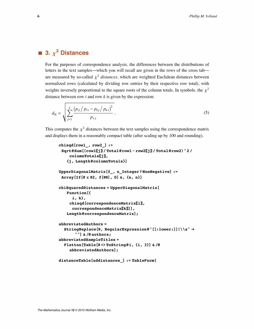
For the purposes of correspondence analysis, the differences between the distributions ofletters in the text samples~which you will recall are given in the rows of the cross tab~are measured by so-called c2 distances, which are weighted Euclidean distances betweennormalized rows (calculated by dividing row entries by their respective row total), withweights inversely proportional to the square roots of the column totals. In symbols, the c2
distance between row i and row k is given by the expression:
(5)dik = ‚j=1
J Ipi j ë pi+ - pk j ë pk+M2
p+ j.
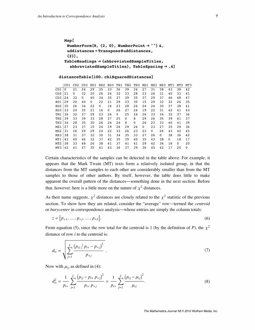
This computes the c2 distances between the text samples using the correspondence matrixand displays them in a reasonably compact table (after scaling up by 100 and rounding).
Certain characteristics of the samples can be detected in the table above. For example, itappears that the Mark Twain (MT) texts form a relatively isolated group, in that thedistances from the MT samples to each other are considerably smaller than from the MTsamples to those of other authors. By itself, however, the table does little to makeapparent the overall pattern of the distances~something done in the next section. Beforethat, however, here is a little more on the nature of c2 distances.
As their name suggests, c2 distances are closely related to the c2 statistic of the previoussection. To show how they are related, consider the “average” row~termed the centroidor barycenter in correspondence analysis~whose entries are simply the column totals:
(6)z = Ap+1, …, p+ j, …, p+JE.
From equation (5), since the row total for the centroid is 1 (by the definition of P), the c2
distance of row i to the centroid is:
(7)diz = ‚j=1
J Ipi j ë pi+ - p+ jM2
p+ j.
Now with mi j as defined in (4):
(8)diz2 =1
pi+‚j=1
J Ipi j - pi+ p+ jM2
pi+ p+ j=
1
pi+‚j=1
J Ipi j - mi jM2
mi j.
Drawing an analogy with the physical concept of angular inertia, correspondence analysisdefines the inertia of a row as the product of the row total (which is referred to as therow’s mass) and the square of its distance to the centroid, pi+ diz2 . Comparing the expres-
sion for diz2 in (5) with definition of the c2 statistic in (3), it follows that the total inertia of
all the rows in a contingency matrix is equal to the c2 statistic divided by n, a quantityknown as Pearson’s mean-square contingency, denoted f2:
(9)‚i=1
I
pi+ diz2 =X2
n= f2.
The total inertia of a table is used to assess the quality of its graphical representation in cor-respondence analysis. For future reference, we can calculate f2 for our dataset.
Correspondence analysis provides a means of representing a table of c2 distances in agraphical form, with rows represented by points, so that the distances between points ap-proximate the c2 distances between the rows they represent.
To compute such a representation, we begin with a matrix of standardized residuals,which are the square roots of the terms comprising the c2 statistic in (3):
(10)W = Bpi j - mi j
mi j
F.
Next, we compute the singular value decomposition of W, which is to say that we find or-thogonal matrices V and W, together with a diagonal matrix L, such that (with the trans-pose of matrix M denoted MT, and writing I for the identity matrix):
(11)W = V L WT,V VT = W WT = I.
The scores of the rows~whose interpretation we discuss later~are given by theexpression:
(12)R = dr V L.
Here dr is the diagonal matrix comprising the reciprocals of the square roots of the rowtotals:
Here dr is the diagonal matrix comprising the reciprocals of the square roots of the rowtotals:
(13)dr =
1
p1+0 0
0 0
0 0 1
pI+
.
The scores of the rows in our sample cross tab are computed in the following (left multipli-cation by dr being more conveniently carried out in Mathematica by row-wise division).
The row scores may be thought of as the coordinates of points in a high-dimensionalspace (14-dimensional, as it turns out in this case).
MatrixRankrowScores
14
These points are arranged so that the Euclidean distance between two points is equal tothe c2 distance between the two rows to which they correspond. To show how the c2 dis-tances between the rows are reflected in their scores, the following reconstitutes the c2 dis-tances in the previous section from Euclidean distances between the scores computedabove. As you can see, the c2 distances are recovered perfectly.
Although the row scores faithfully reproduce the c2 distances between rows in theoriginal table, as coordinates their dimensionality is far too high for them to be presentedgraphically. Thanks to the properties of the singular value decomposition, however, takingjust the first two components of each row’s score usually produces a reasonable approxi-mation to the c2 distances, and yields coordinates that can be placed on a two-dimen-sional plot. (Below we have labeled the components “X” and “Y” to highlight their role as2D coordinates.)
CD Charles DarwinRD Rene DescartesTH Thomas HobbesMS Mary ShelleyMT Mark Twain
Ú Figure 1. Row plot for text samples.
The plot gives a much clearer picture of the way in which the letters are distributed acrossthe text samples. For example, it is quite evident that~as we concluded from the originalcross tab~the Mark Twain samples differ significantly as a group from those of the otherwriters. The text samples of Darwin and Hobbes also appear to be sui generis, though theDescartes and Shelly samples appear less distinct. The plot suggests that it may be possi-ble, therefore, to distinguish between the works of at least some of the authors using corre-spondence analysis of their letter distributions.
Since it uses only the first two components of the row scores, the plot above only approx-imates the true configuration of the rows in the cross tab. Before using it to make firminferences, we might try to gauge the quality of the representation it provides. Oneindicator is derived from the inertia of the rows defined in (9). Recall that f2, the totalinertia of the rows, is calculated from the row totals and the c2 distances of the rows tothe centroid:
(14)f2 = ‚i=1
I
pi+ diz2 .
It may be shown that for any contingency matrix, the procedure of the previous section al-ways places the centroid at the origin of the plot. Therefore, since Euclidean distances onthe plot are supposed to approximate c2 distances, replacing each c2 distance diz in theright-hand side of (14) by the distance of the corresponding row point to origin shouldyield an approximation to f2. The following derives this quantity and computes its ratio tothe true value of f2.
Thus our two-dimensional plot captures about 56% of the total inertia of the table rows.While this seems hardly an impressive fraction, Murtagh ([3], p. 39) points out that ratioslike this are not uncommon in correspondence analysis, and do not necessarily point to abad representation. Nonetheless, we might want to exercise a modicum of caution beforedrawing categorical conclusions from our analysis.
As an aside, it turns out that the total inertia of the contingency matrix P~which wascalculated “longhand” in (9)~is equal to the sum of the squares of the diagonal elementsof the matrix L in (11). The latter comprise the singular values of the matrix W.Furthermore, the inertia retained in the two-dimensional plot is simply the sum of thesquares of the first two singular values in L. Thus the following is an equivalentexpression of the plot’s inertia.
‡ 6. Plotting ColumnsWe have seen how correspondence analysis can be used to derive a visual representationof the relationships between the rows of a contingency matrix. We can also use correspon-dence analysis to illustrate the relationship between the rows and the columns of a corre-spondence matrix~between the texts and letters in our example. Since our primary con-cern is with the text samples, the rows of the cross tab, it might seem a digression to lookat the cross tab columns (the characters appearing in the texts), but we will see in the nextsection that the geometry of the columns is central to the identification of the mysterytexts.
As with the rows, we begin by deriving scores for the columns from the singular value de-composition in (11). With reference to (11), the matrix C, whose rows are the columnscores, is calculated as follows:
(15)C = Dc W,
where
(16)dc =
1
p+10 0
0 0
0 0 1
p+J
.
Again, left multiplication by the diagonal matrix dc is more conveniently expressed as ele-ment-wise division in Mathematica.
We can display both columns and rows on the same plot with a slight elaboration of themethod used to plot the rows alone. The column coordinates are scaled so that the columnpoints occupy roughly the same region of the plot as the row points.
CD Charles DarwinRD Rene DescartesTH Thomas HobbesMS Mary ShelleyMT Mark Twain
Ú Figure 2. Row and column plot for text samples.
Interpreting the relationships between rows and columns from a plot such as this is not asstraightforward as it was for the previous plot with the rows only. For example, it is nottrue in general that the closer a column appears to a row, the greater the prevalence of thecorresponding letter in the corresponding text sample.
To show how such relationships are actually represented, consider the text sample “MT2”(a row) and characters “P” and “Y” (columns).
Possibly the simplest way to determine the relationship between a text sample and acharacter is to draw lines from their corresponding points in the plot to the origin. If theangle between the two lines is acute, then the character occurs more often in the samplethan it does on average in the texts as a whole. Conversely, if the angle is obtuse, thecharacter occurs less often than overall. The following draws the appropriate lines for ourchosen text sample and characters; it appears the character “Y” occurs more often thanaverage in “MT2”, while “P” occurs less often.
Unfortunately, the method described above only tells us if a character appears more orless often than average in a text sample, not whether one character appears more oftenthan another in a sample. In particular, an angle that is more acute does not signify a char-acter that is more prevalent in a text.
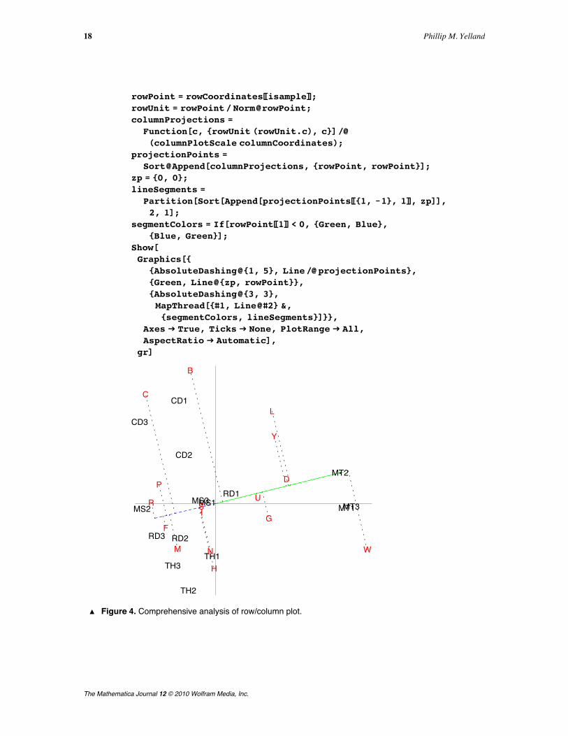
A rather more complicated method that does illustrate the relative frequencies of charac-ters in a text sample entails first drawing a line on the plot through the origin and the pointcorresponding to the text sample in question. Perpendiculars to this line are dropped fromeach character’s position on the plot. The following draws such a construction for the se-lected text sample “MT2”.
Ú Figure 4. Comprehensive analysis of row/column plot.
The relative frequencies of the characters in the text sample can be read off by traversingthe line through the text sample (colored blue and green on the plot above), looking at thepositions at which the perpendiculars from the characters intersect it. A character with anintersection on the green line segment (i.e., on the same side of the origin as the text sam-ple) occurs more often in the sample than the average in the texts overall, whereas one onthe blue line segment (on the other side of the origin) occurs less frequently than the aver-age. In addition, the further from the origin on the green line segment such an intersectionoccurs, the greater the frequency of the character in the sample. Conversely, the furtherout on the blue segment an intersection falls, the less frequent the character in the sample.
The relative frequencies of the characters in the text sample can be read off by traversingthe line through the text sample (colored blue and green on the plot above), looking at thepositions at which the perpendiculars from the characters intersect it. A character with anintersection on the green line segment (i.e., on the same side of the origin as the text sam-ple) occurs more often in the sample than the average in the texts overall, whereas one onthe blue line segment (on the other side of the origin) occurs less frequently than the aver-age. In addition, the further from the origin on the green line segment such an intersectionoccurs, the greater the frequency of the character in the sample. Conversely, the furtherout on the blue segment an intersection falls, the less frequent the character in the sample.
So from the plot above, it appears that the character “W” occurs most often in the sampletext, and that characters “L”, “D”, “Y”, “G”, “U”, “B”, “S”, “I”, “N”, “H”, “C”, “M”, “P”,“F”, and “R” occur successively less often; characters “W” through “B” in the ranking ap-pear more often than average, while “S” through “R” appear less often than average.
‡ 7. Supplementary Points: Identifying the Mystery TextsFinally, we return to the problem we faced at the outset: identifying the author or authorsof the unidentified text fragments. We have seen how the application of simple correspon-dence analysis to the text samples allows us to view them graphically in terms of their let-ter distributions. In Section 5 we saw that it was generally possible to distinguish the au-thors of the text samples based upon the locations of the corresponding row points~witha few exceptions, samples of work by the same writer tended to occupy the same area ofthe plot. One might logically surmise that if we were to plot the mystery texts on the samecorrespondence plot as the samples, we would be able to determine their authorship bylooking at the authors of the nearest samples. To begin, we need to calculate an additionalcross tab containing the distribution of the selected characters in the mystery texts.
mysteryTextXTitles "TextX1", "TextX2";TableFormmysteryTextTab,TableHeadings mysteryTextXTitles, chars,TableSpacing .5, TableAlignments Center
B C D F G H I L M N P R S U W YTextX1 24 26 80 17 32 91 86 54 32 91 19 58 93 50 58 30TextX2 19 33 35 22 40 96 116 39 40 129 17 72 104 30 25 24
We could proceed by simply appending these frequencies as new rows to the original textsamples cross tab given in Section 1 and recalculating the scores and coordinates for allthe rows (that is, both the original samples and the mystery texts) in the resulting table. Inprinciple, however, it is possible that the unidentified texts overlap one or more of the textsamples, and if this were the case, appending the new rows to the cross tab would distortthe analysis by “double-counting” some of the samples.
We could proceed by simply appending these frequencies as new rows to the original textsamples cross tab given in Section 1 and recalculating the scores and coordinates for allthe rows (that is, both the original samples and the mystery texts) in the resulting table. Inprinciple, however, it is possible that the unidentified texts overlap one or more of the textsamples, and if this were the case, appending the new rows to the cross tab would distortthe analysis by “double-counting” some of the samples.
A more satisfactory approach derives from the fact that the row scores computed in Sec-tion 4 are actually weighted sums of the column scores calculated in Section 6. In matrixterms, recalling that P is the correspondence matrix and C is the matrix of column scores,it can be shown that:
(17)R = dr2 P C,
where
(18)dr2 = dr dr =
1p1+
0 0
0 0
0 0 1pI+
.
If we replace the original correspondence matrix P in (17) with a new correspondence ma-trix formed from the cross tab of the unidentified texts, we derive a set of row scores forthe unidentified texts according to the transformation determined by the text samples only(since they alone produced the row scores C), eliminating the risk of double-counting.Treated in this way, the unidentified texts comprise supplementary points in the terminol-ogy of correspondence analysis.
The following calculates row scores for the mystery texts as supplementary points(straightforward algebra vindicates the direct use of the new cross tab without the need toderive a new correspondence matrix).
mysteryTextScores mysteryTextTab.columnScores Total mysteryTextTab
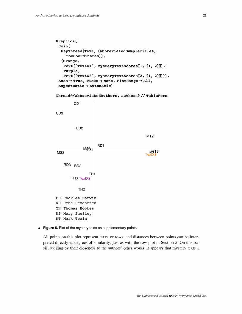
Lastly, as with the rows and columns, we take the first two elements of the scores aboveto produce the coordinates of the supplementary points. In the following, they are dis-played on the same plot as the original rows.
CD Charles DarwinRD Rene DescartesTH Thomas HobbesMS Mary ShelleyMT Mark Twain
Ú Figure 5. Plot of the mystery texts as supplementary points.
All points on this plot represent texts, or rows, and distances between points can be inter-preted directly as degrees of similarity, just as with the row plot in Section 5. On this ba-sis, judging by their closeness to the authors’ other works, it appears that mystery texts 1and 2 belong to Mark Twain and Thomas Hobbes respectively. While the manifest isola-tion of the Mark Twain texts on the plot leaves little doubt as to the provenance of the firstunidentified text, the author of the second is a little less clearly defined~particularlygiven the middling diagnostic ratio calculated in Section 5. Nonetheless, I am sure youwill agree that considering the rather scant literary information on which the analysis wasbased (amounting to no more than a table of letter frequencies), the results areencouraging.
All points on this plot represent texts, or rows, and distances between points can be inter-preted directly as degrees of similarity, just as with the row plot in Section 5. On this ba-
and 2 belong to Mark Twain and Thomas Hobbes respectively. While the manifest isola-tion of the Mark Twain texts on the plot leaves little doubt as to the provenance of the firstunidentified text, the author of the second is a little less clearly defined~particularlygiven the middling diagnostic ratio calculated in Section 5. Nonetheless, I am sure youwill agree that considering the rather scant literary information on which the analysis wasbased (amounting to no more than a table of letter frequencies), the results areencouraging.
‡ 8. ConclusionCorrespondence analysis has a long and storied history that can be traced as far back asthe 1930s. We have only scratched the surface of the subject in this brief introductoryarticle. Of course, I have omitted proofs of the various assertions I have made in thecourse of the presentation. Furthermore, I have glossed over an important choiceconcerning the scaling of row and column scores and coordinates; I have used so-calledrow principal scoring (which preserves c2 distances between rows, but not columns), butthere are other approaches that are equally valid.
A number of extensions exist to the so-called simple correspondence analysis presentedhere. Most important are multiple and joint correspondence analysis, which apply tocontingency tables involving three or more variables or sets of categories (see [4] fordetails). For a comprehensive examination of correspondence analysis and related tech-niques, Greenacre’s early book [5] remains among the best texts (in the English language,at least), though it is unfortunately currently out of print. Later books by Greenacre [6]and coeditor Blasius [7] explore applications of correspondence analysis and extensions tothe basic methodology. Benzécri’s treatise [8] is notable in that its author championed theuse of correspondence analysis for many years, developing many of the geometric under-pinnings that inform modern practice and establishing a seminal school of statisticalanalysis in France; unfortunately, translation from the original French and a prodigiousprice detract from the appeal of the text itself. Most recently, Murtagh [3] gives athorough (if somewhat telegraphic) treatment of the subject, with an emphasis on thecoding of data for analysis. Sections devoted to correspondence analysis also appear in thebooks by Agresti [9], Borg and Groenen [10], and Legendre and Legendre [11].
In his forward to [3], Benzécri writes of the immense opportunities afforded statisticiansby “inexpensive means of computation that could not be dreamed of just thirty years ago”(indeed, correspondence analysis of realistically sized datasets is all but impossiblewithout a computer). I hope that this article has demonstrated that Mathematica can play avaluable role in allowing all of us~statistician and non-statistician alike~to takeadvantage of these opportunities.
‡ References[1] D. W. Foster, Author Unknown: Tales of a Literary Detective, New York: Henry Holt & Com-
pany, 2001.
[2] [J. Klein], Primary Colors: A Novel of Politics, New York: Random House, 1996.
[3] F. Murtagh, Correspondence Analysis and Data Coding with Java and R, Boca Raton: Chap-man & Hall/CRC, 2005.
[4] M. J. Greenacre, “Multiple and Joint Correspondence Analysis,” Correspondence Analysis inthe Social Sciences (M. J. Greenacre and J. Blasius, eds.), London: Academic Press, 1994pp. 141|161.
[5] M. J. Greenacre, Theory and Applications of Correspondence Analysis, London: AcademicPress, 1984.
[6] M. J. Greenacre, Correspondence Analysis in Practice, London: Academic Press, 1993.
[7] M. J. Greenacre and J. Blasius, eds., Correspondence Analysis in the Social Sciences: Re-cent Developments and Applications, London: Academic Press, 1994.
[8] J. P. Benzécri, Correspondence Analysis Handbook, New York: Marcel Dekker, 1992.
[9] A. Agresti, Categorical Data Analysis, 2nd ed., New York: Wiley, 2002.
[10] I. Borg and P. Groenen, Modern Multidimensional Scaling: Theory and Applications, NewYork: Springer, 1997.
[11] P. Legendre and L. Legendre, Numerical Ecology, 2nd English ed., New York: Elsevier Sci-ence, 1998.
P. Yelland, “An Introduction to Correspondence Analysis,” The Mathematica Journal, 2010. dx.doi.org/doi:10.3888/tmj.12|4.
About the Author
Phillip Yelland is a data analyst at Facebook, Inc., where his work centers on the use ofstatistical techniques in fraud detection and risk management. He has an M.A. and a Ph.D.in computer science from the University of Cambridge in England, and an M.B.A. fromthe University of California at Berkeley.Phillip YellandFacebook, Inc.1601 South California AvenuePalo Alto, CA [email protected]