THE MATHEMATICS OF GRAVITATIONAL WAVES ... MATHEMATICS OF GRAVITATIONAL WAVES This illustration...

THE MATHEMATICS OF GRAVITATIONAL WAVES

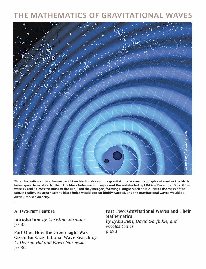
This illustration shows the merger of two black holes and the gravitational waves that ripple outward as the black holes spiral toward each other. The black holes—which represent those detected by LIGO on December 26, 2015—were 14 and 8 times the mass of the sun, until they merged, forming a single black hole 21 times the mass of the sun. In reality, the area near the black holes would appear highly warped, and the gravitational waves would be difficult to see directly.

Cou

rtes

y of

LIG

O/T

. Pyl

e.

A Two-Part Feature

Introduction by Christina Sormanip 685

Part One: How the Green Light Was Given for Gravitational Wave Search by C. Denson Hill and Paweł Nurowski p 686

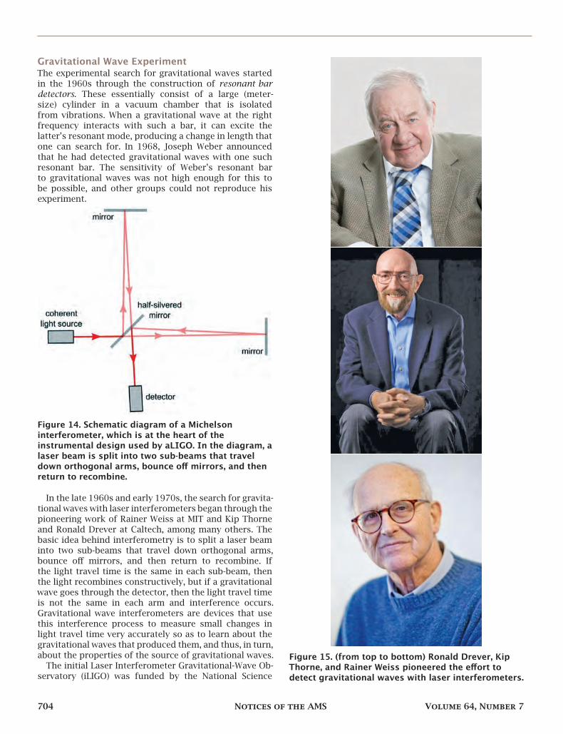
Part Two: Gravitational Waves and Their Mathematics by Lydia Bieri, David Garfinkle, and Nicolás Yunes p 693

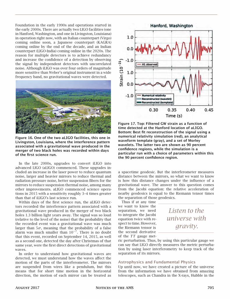
Our second article, by Lydia Bieri, David Garfinkle, and Nicolás Yunes, describes the mathematics behind gravitational waves in more detail, beginning with a description of the geometry of spacetime. They discuss Choquet-Bruhat’s famous 1952 proof of ex-istence of solutions to the Einstein equations given Cauchy data. They then proceed to the groundbreak-ing work of Christodoulou-Klainerman and a descrip-tion of the theory behind gravitational radiation: the radiation of energy in the form of gravitational waves.

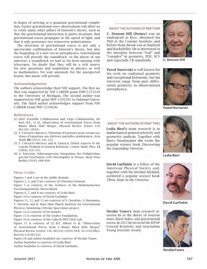
Numerical methods are used to predict the gravi-tational waves emanating from specific cosmological events like the collision of black holes. Starting in Section 4 of their article, Bieri et al. describe these numerical methods beginning with linearized theory and the post-Newtonian approximation first devel-oped by Einstein. They then describe the inward spiraling (as on the cover of this issue) of two black holes coming together and the resulting waves that occur as the black holes merge into one. They close with a description of the LIGO detector and how its measurements corroborated the predictions of the numerical teams. Ultimately the LIGO detection of gravitational waves not only validated Einstein’s theory of general relativity, but also the work of the many mathematicians who contributed to an under-standing of this theory.

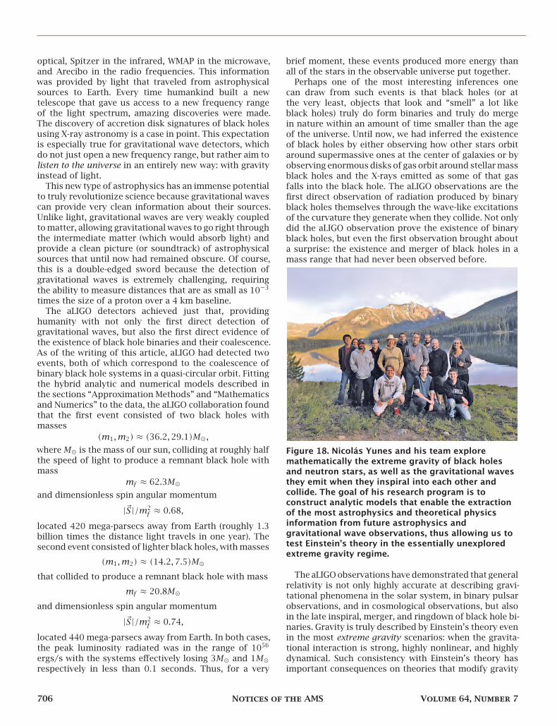
Our second article, by Lydia Bieri, David Garfinkle, and Nicolás Yunes, describes the mathematics behind gravitational waves in more detail, beginning with a description of the geometry of spacetime. They discuss Choquet-Bruhat’s famous 1952 proof of ex-istence of solutions to the Einstein equations given Cauchy data. They then proceed to the groundbreak-ing work of Christodoulou-Klainerman and a descrip-tion of the theory behind gravitational radiation: the radiation of energy in the form of gravitational waves.

Numerical methods are used to predict the gravi-tational waves emanating from specific cosmological events like the collision of black holes. Starting in Section 4 of their article, Bieri et al. describe these numerical methods beginning with linearized theory and the post-Newtonian approximation first devel-oped by Einstein. They then describe the inward spiraling (as on the cover of this issue) of two black holes coming together and the resulting waves that occur as the black holes merge into one. They close with a description of the LIGO detector and how its measurements corroborated the predictions of the numerical teams. Ultimately the LIGO detection of gravitational waves not only validated Einstein’s theory of general relativity, but also the work of the many mathematicians who contributed to an under-standing of this theory.

Introduction by Christina SormaniThe Mathematics of Gravitational WavesA little over a hundred years ago, Albert Einstein predicted the existence of gravitational waves as a possible consequence of his theory of general relativ-ity. Two years ago, these waves were first detected by LIGO. In this issue of Notices we focus on the mathematics behind this profound discovery.

Einstein’s prediction of gravitational waves was based upon a linearization of his gravitational field equations, and he did not believe they existed as solutions to the original nonlinear system of equa-tions. It was not until the 1950s that the mathemat-ics behind Einstein’s gravitational field equations was understood well enough even to define a wave solution. Robinson and Trautman produced the first family of explicit wave solutions to Einstein’s non-linear equations in 1962. Our first article, written by C. Denson Hill and Paweł Nurowski, describes thisstory of how the theoretical existence of gravitational waves was determined.

Christina Sormani is a Notices editor. Her e-mail address is [email protected].

For permission to reprint this article, please contact: [email protected].

DOI: http://dx.doi.org/10.1090/noti1551

Part one by C. Denson Hill andPaweł Nurowski

How the Green Light Was Given for Gravita-tional Wave SearchThe recent detection of gravitational waves by theLIGO/Virgo team (B. P. Abbot et al. 2016) is an in-credibly impressive achievement of experimental physics.It is also a tremendous success of the theory of generalrelativity. It confirms the existence of black holes, showsthat binary black holes exist and that theymay collide, andthat during the merging process gravitational waves areproduced. These are all predictions of general relativitytheory in its fully nonlinear regime.

The existence of gravitational waves was predicted byAlbert Einstein in 1916within the framework of linearizedEinstein theory. Contrary to common belief, even the verydefinition of a gravitational wave in the fully nonlinearEinstein theory was provided only after Einstein’s death.Actually, Einstein advanced erroneous arguments againstthe existence of nonlinear gravitational waves, whichstopped the development of the subject until the mid1950s. This is what we refer to as the red light forgravitational wave research.

In this note we explain how the obstacles concerninggravitational wave existence were successfully overcomeat the beginning of the 1960s, giving the green lightfor experimentalists to start designing detectors, whicheventually produced the recent LIGO/Virgo discovery.

Gravitational Waves in Einstein’s LinearizedTheoryThe idea of a gravitational wave comes directly fromAlbert Einstein. Immediately after formulating GeneralRelativity Theory, still in 1916 Einstein [3] linearized hisfield equations(0.1) 𝑅𝜇𝜈 − 1

2𝑅𝑔𝜇𝜈 = 𝜅𝑇𝜇𝜈

by assuming that the metric 𝑔𝜇𝜈 representing the gravita-tional field has the form of a slightly perturbedMinkowskimetric 𝜂𝜇𝜈,

𝑔𝜇𝜈 = 𝜂𝜇𝜈 + 𝜖ℎ𝜇𝜈.Here 0 < 𝜖 ≪ 1, and his linearization simply means thathe developed the left hand side of (0.1) in powers of 𝜖 and

C. Denson Hill is professor of mathematics at Stony Brook Univer-sity. His e-mail address is [email protected].

Paweł Nurowski is professor of physics at the Center for Theoreti-cal Physics of the Polish Academy of Sciences. His e-mail addressis [email protected].

This article is an abbreviated version of the arXiv article athttps://arxiv.org/pdf/1608.08673.

This work was supported in part by the Polish Ministry of Scienceand Higher Education under the grant 983/P-DUN/2016.

For permission to reprint this article, please contact:

[email protected]: http://dx.doi.org/10.1090/noti1550

neglected all terms involving 𝜖𝑘 with 𝑘 > 1. As a resultof this linearization Einstein found the field equations oflinearized general relativity, which can conveniently bewritten for an unknown

ℎ𝜇𝜈 = ℎ𝜇𝜈 − 12𝜂𝜇𝜈ℎ𝛼𝛽𝜂𝛼𝛽

as□ℎ𝜇𝜈 = 2𝜅𝑇𝜇𝜈, □ = 𝜂𝜇𝜈𝜕𝜇𝜕𝜈.

These equations, outside the sources where𝑇𝜇𝜈 = 0,

constitute a system of decoupled relativistic wave equa-tions(0.2) □ℎ𝜇𝜈 = 0for each component of ℎ𝜇𝜈. This enabled Einstein toconclude that linearized general relativity theory admitssolutions in which the perturbations of Minkowski space-time ℎ𝜇𝜈 are plane waves traveling with the speed of light.Because of the linearity, by superposing plane wave solu-tions with different propagation vectors 𝑘𝜇, one can getwaves having any desirable wave front. Einstein namedthese gravitational waves. He also showed that within thelinearized theory these waves carry energy, and he founda formula for the energy loss in terms of the third timederivative of the quadrupole moment of the sources.

Since far from the sources the gravitational field isvery weak, solutions from the linearized theory shouldcoincide with solutions from the full theory. Actually thewave detected by the LIGO/Virgo team was so weak thatit was treated as if it were a gravitational plane wave fromthe linearized theory. We also mention that essentiallyall visualizations of gravitational waves presented duringpopular lectures or in the news are obtained usinglinearized theory only.

The Red LightWe focus here on the fundamental problem posed byEinstein in 1916, which bothered him to the end of his life.The problem is: Do the fully nonlinear Einstein equationsadmit solutions that can be interpreted as gravitationalwaves?

If “yes,” then far from the sources, it is entirely reason-able to use linearized theory. If “no,” then it makes nosense to expend time, effort, and money to try to detectsuch waves: solutions from the linearized theory are notphysical; they are artifacts of the linearization.

If the answer is “no” we refer to it as a “red light” forgravitational wave search. This red light can be switchedto “green” only if the following subproblems are solved:

(1) What is a definition of a plane gravitational wavein the full theory?

(2) Does the so defined plane wave exist as a solutionto the full Einstein system?

(3) Do such waves carry energy?(4) What is a definition of a gravitational wave with

nonplanar front in the full theory?(5) What is the energy of such waves?(6) Do there exist solutions to the full Einstein system

satisfying this definition?

686 Notices of the AMS Volume 64, Number 7

https://arxiv.org/pdf/1608.08673

(7) Does the full theory admit solutions correspond-ing to the gravitational waves emitted by boundedsources?

To give a green light here, one needs a satisfactory answerto all these subproblems. Let us explain: Suppose that onlythe questions (1)–(3) had been settled in a satisfactorymanner. Could we have a green light? The answer is no,because, contrary to the linear theory, unless we are verylucky, there is no way of superposing plane waves toobtain waves with arbitrary fronts. Thus the existenceof a plane wave does not mean the existence of wavesthat can be produced by bounded sources, such as forexample binary black hole systems.

Search for Plane Waves in the Full TheoryNaive ApproachAnaive answer to our question (1) could be: a gravitationalplane wave is a spacetime described by a metric, whichin some coordinates (𝑡, 𝑥, 𝑦, 𝑧), with 𝑡 being timelike, hasmetric functions depending on 𝑢 = 𝑡− 𝑥 only; preferablythese functions should be sin or cos. This is not a goodapproach as is seen in the following example:

Consider the metric𝑔 =(𝜂𝜇𝜈 +ℎ𝜇𝜈)d𝑥𝜇d𝑥𝜈 = d𝑡2 − d𝑥2 − d𝑦2 − d𝑧2

+ cos(𝑡 − 𝑥)(2 + cos(𝑡 − 𝑥))d𝑡2

− 2 cos(𝑡 − 𝑥)(1 + cos(𝑡 − 𝑥))d𝑡d𝑥+ cos2(𝑡 − 𝑥)d𝑥2.

We see here that the terms after the first row give theperturbation ℎ𝜇𝜈d𝑥𝜇d𝑥𝜈 of the Minkowski metric 𝜂 =𝜂𝜇𝜈d𝑥𝜇d𝑥𝜈 = d𝑡2 − d𝑥2 − d𝑦2 − d𝑧2. They are oscillatory,and one sees that the ripples of the perturbationmove withthe speed of light, 𝑐 = 1, along the 𝑥-axis. A closer lookshows also that the coefficients ℎ𝜇𝜈 of the perturbationsatisfy the wave equation (0.2) (since they depend on asingle null coordinate 𝑢 only), and more importantly, thatthe full metric 𝑔 has Ricci curvature 0 (is “Ricci flat”).

Thus the above metric is not only an example of a“gravitational wave” in the linearized Einstein theory, butalso it provides an example of a solution of the vacuumEinstein equations 𝑅𝜇𝜈 = 0 in the fully nonlinear Einsteintheory. With all this information in mind, in particularhaving in mind the sinusoidal change of the metric withthe speed of light in the 𝑥 direction, we ask: is this anexample of a plane gravitational wave?

The answer is no, as we created the metric 𝑔 from theflat Minkowski metric 𝜂 = d 𝑡2 − d𝑥2 − d𝑦2 − d𝑧2 by achange of the time coordinate: 𝑡 = 𝑡 + sin(𝑡 − 𝑥). In viewof this, the metric 𝑔 is just the flat Minkowski metric,written in nonstandard coordinates. As such it does notcorrespond to any gravitational wave!

The moral from this example is that attaching thename of a “gravitational wave” to a spacetime that justsatisfies an intuitive condition in some coordinate systemis a wrong approach. As we see in this example we canalways introduce a sinusoidal behaviour of the metriccoefficients and their ‘movement’ with speed of light, byan appropriate change of coordinates.

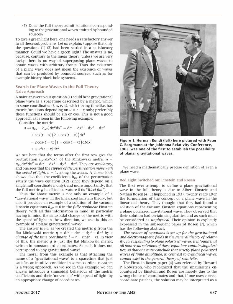
Figure 1. Herman Bondi (left) here pictured with PeterG. Bergmann at the Jabłonna Relativity Conference,1962, was one of the first to establish the possibilityof planar gravitational waves.

We need a mathematically precise definition of even aplane wave.

Red Light Switched on: Einstein and RosenThe first ever attempt to define a plane gravitationalwave in the full theory is due to Albert Einstein andNathan Rosen [4]. It happened in 1937, twenty years afterthe formulation of the concept of a plane wave in thelinearized theory. They thought that they had found asolution of the vacuum Einstein equations representinga plane polarized gravitational wave. They observed thattheir solution had certain singularities and as such mustbe considered as unphysical. Their opinion is explicitlyexpressed in the subsequent paper of Rosen [7], whichhas the following abstract:

The system of equations is set up for the gravitationaland electromagnetic fields in the general theory of relativ-ity, corresponding to plane polarized waves. It is found thatall nontrivial solutions of these equations contain singulari-ties, so that one must conclude that strictly plane polarizedwaves of finite amplitude, in contrast to cylindrical waves,cannot exist in the general theory of relativity.

The Einstein-Rosen paper [4] was refereed by HowardP. Robertson, who recognized that the singularities en-countered by Einstein and Rosen are merely due to thewrong choice of coordinates and that, if one uses correctcoordinate patches, the solution may be interpreted as a

August 2017 Notices of the AMS 687

cylindrical wave, which is nonsingular everywhere excepton the symmetry axis corresponding to an infinite linesource. This is echoed in Rosen’s abstract quoted abovein his phrase “in contrast to cylindrical waves,” and is alsomentioned in the abstract of the earlier Einstein-Rosenpaper [4], whose first sentence is: The rigorous solutionfor cylindrical gravitational waves is given. Nevertheless,despite the clue given to them by Robertson, starting from1937, neither Einstein nor Rosen believed that physicallyacceptable plane gravitational waves were admitted bythe full Einstein theory. This belief of Einstein affectedthe views of his collaborators, such as Leopold Infeld,and more generally many other relativists. If a planegravitational wave is not admitted by the theory, and ifthis statement comes from, and is fully supported by,the authority of Einstein, it was hard to believe at anyfundamental level that the predictions of the linearizedtheory were valid.

Towards the Green Light: Bondi, Pirani, and RobinsonIt is now fashionable to say that a new era of research ongravitational waves started at the International Confer-ence on Gravitation held at Chapel Hill on 18–23 January1957. To show that not everybody was sure about theexistence of gravitational waves during this conferencewe quote Herman Bondi [1], one of the founding fathersof gravitational wave theory:

Polarized plane gravitational waves were first discov-ered by N. Rosen, who, however, came to the conclusionthat such waves could not exist because the metric wouldhave to contain certain physical singularities. More recentwork by Taub and McVittie showed that there were nounpolarized plane waves, and this result has tended toconfirm the view that true plane gravitational waves donot exist in empty space in general relativity. Partly owingto this, Scheidegger and I have both expressed the opin-ion that there might be no energy-carrying gravitationalwaves at all in the theory.

The last sentence in the quote refers to Bondi’s opinionexpressed during the Chapel Hill Conference. Interest-ingly, the quote is from Bondi’s Nature paper announcingthe discovery of a singularity-free solution of a planegravitational wave that carries energy, received by thejournal on March 24, 1957. A dramatic change of opinionbetween January and March of the same year!

Bondi in the Nature paper invokes the solution ofEinstein’s equations found in the context of gravitationalwaves by Ivor Robinson. This paper, and the subsequentpaper written by Bondi, Felix Pirani, and Robinson [2],answers in positive our problems (1), (2), and (3).

Inparticular (1) is answeredwith the followingdefinitionof a plane wave in the full theory: The gravitational planewave is a spacetime that (a) satisfies vacuum Einstein’sequations 𝑅𝜇𝜈 = 0 and (b) has a 5-dimensional group ofisometries. The motivation for this definition is the factthat a plane electromagnetic wave has a 5-dimensionalgroup of symmetries. Bondi, Pirani, and Robinson do notassume that the 5-dimensional group of isometries isisomorphic to the symmetry of a plane electromagneticwave. They inspect all Ricci flat metrics with symmetries

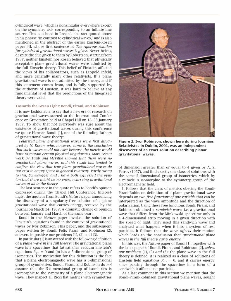
Figure 2. Ivor Robinson, shown here during JournéesRelativistes in Dublin, 2001, was an independentdiscoverer of an exact solution describing planargravitational waves.

of dimension greater than or equal to 4 given by A. Z.Petrov (1957), and find exactly one class of solutions withthe same 5-dimensional group of isometries, which bya miracle is isomorphic to the symmetry group of theelectromagnetic field.

It follows that the class of metrics obeying the Bondi-Pirani-Robinson definition of a plane gravitational wavedepends on two free functions of one variable that can beinterpreted as the wave amplitude and the direction ofpolarization. Using these free functions Bondi, Pirani, andRobinson obtained a sandwich wave, i.e. a gravitationalwave that differs from the Minkowski spacetime only ina 4-dimensional strip moving in a given direction withthe speed of light. They used this sandwich wave andanalyzed what happens when it hits a system of testparticles. It follows that the wave affects their motion,which leads to the conclusion that gravitational planewaves in the full theory carry energy.

In this way, the Nature paper of Bondi [1], together withthe later paper of Bondi, Pirani, and Robinson [2], solvesour problems (1), (2) and (3): the plane wave in the fulltheory is defined, it is realized as a class of solutions ofEinstein field equations 𝑅𝜇𝜈 = 0, and it carries energy,since passing through the spacetime in a form of asandwich it affects test particles.

As a last comment in this section we mention that theBondi-Pirani-Robinson gravitational plane waves, sought


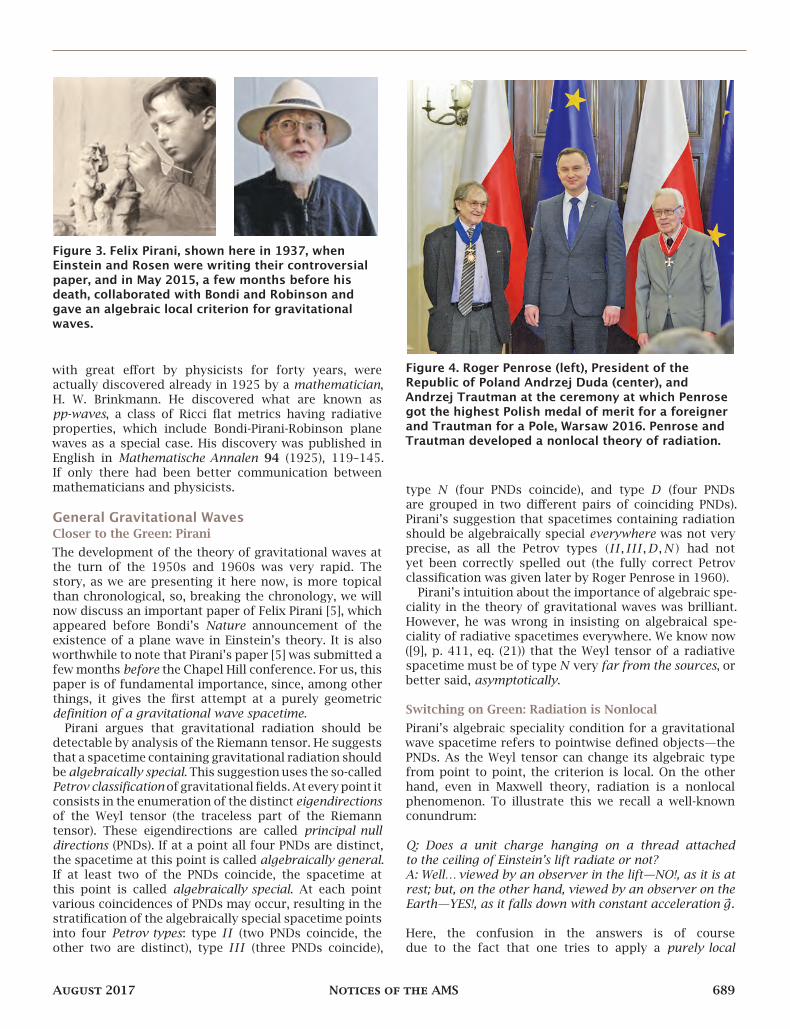
Figure 3. Felix Pirani, shown here in 1937, whenEinstein and Rosen were writing their controversialpaper, and in May 2015, a few months before hisdeath, collaborated with Bondi and Robinson andgave an algebraic local criterion for gravitationalwaves.

with great effort by physicists for forty years, wereactually discovered already in 1925 by a mathematician,H. W. Brinkmann. He discovered what are known aspp-waves, a class of Ricci flat metrics having radiativeproperties, which include Bondi-Pirani-Robinson planewaves as a special case. His discovery was published inEnglish in Mathematische Annalen 94 (1925), 119–145.If only there had been better communication betweenmathematicians and physicists.

General Gravitational WavesCloser to the Green: PiraniThe development of the theory of gravitational waves atthe turn of the 1950s and 1960s was very rapid. Thestory, as we are presenting it here now, is more topicalthan chronological, so, breaking the chronology, we willnow discuss an important paper of Felix Pirani [5], whichappeared before Bondi’s Nature announcement of theexistence of a plane wave in Einstein’s theory. It is alsoworthwhile to note that Pirani’s paper [5] was submitted afewmonths before the Chapel Hill conference. For us, thispaper is of fundamental importance, since, among otherthings, it gives the first attempt at a purely geometricdefinition of a gravitational wave spacetime.

Pirani argues that gravitational radiation should bedetectable by analysis of the Riemann tensor. He suggeststhat a spacetime containing gravitational radiation shouldbe algebraically special. This suggestion uses the so-calledPetrov classificationof gravitational fields.At everypoint itconsists in the enumeration of the distinct eigendirectionsof the Weyl tensor (the traceless part of the Riemanntensor). These eigendirections are called principal nulldirections (PNDs). If at a point all four PNDs are distinct,the spacetime at this point is called algebraically general.If at least two of the PNDs coincide, the spacetime atthis point is called algebraically special. At each pointvarious coincidences of PNDs may occur, resulting in thestratification of the algebraically special spacetime pointsinto four Petrov types: type 𝐼𝐼 (two PNDs coincide, theother two are distinct), type 𝐼𝐼𝐼 (three PNDs coincide),

Figure 4. Roger Penrose (left), President of theRepublic of Poland Andrzej Duda (center), andAndrzej Trautman at the ceremony at which Penrosegot the highest Polish medal of merit for a foreignerand Trautman for a Pole, Warsaw 2016. Penrose andTrautman developed a nonlocal theory of radiation.

type 𝑁 (four PNDs coincide), and type 𝐷 (four PNDsare grouped in two different pairs of coinciding PNDs).Pirani’s suggestion that spacetimes containing radiationshould be algebraically special everywhere was not veryprecise, as all the Petrov types (𝐼𝐼, 𝐼𝐼𝐼,𝐷,𝑁) had notyet been correctly spelled out (the fully correct Petrovclassification was given later by Roger Penrose in 1960).

Pirani’s intuition about the importance of algebraic spe-ciality in the theory of gravitational waves was brilliant.However, he was wrong in insisting on algebraical spe-ciality of radiative spacetimes everywhere. We know now([9], p. 411, eq. (21)) that the Weyl tensor of a radiativespacetime must be of type 𝑁 very far from the sources, orbetter said, asymptotically.

Switching on Green: Radiation is NonlocalPirani’s algebraic speciality condition for a gravitationalwave spacetime refers to pointwise defined objects—thePNDs. As the Weyl tensor can change its algebraic typefrom point to point, the criterion is local. On the otherhand, even in Maxwell theory, radiation is a nonlocalphenomenon. To illustrate this we recall a well-knownconundrum:

Q: Does a unit charge hanging on a thread attachedto the ceiling of Einstein’s lift radiate or not?A: Well…viewed by an observer in the lift—NO!, as it is atrest; but, on the other hand, viewed by an observer on theEarth—YES!, as it falls down with constant acceleration 𝑔.

Here, the confusion in the answers is of coursedue to the fact that one tries to apply a purely local


physical law—the equivalence principle1—to the very non-local phenomenon, which is radiation in electromagnetictheory.

This gives a hint as to how to define what radiationis in general relativity. One can not expect that in thisnonlinear theory radiation can be defined in terms of localnotions. This point is raised and consequently developedby Andrzej Trautman, in two papers [8, 9] submitted toBulletin de l’Academie Polonaise des Sciences, behind theIron Curtain, in April 1958. This led him to finally solveour problems (4)–(5), [9], and (6)–(7), [6], thereby switchingthe red light to green.

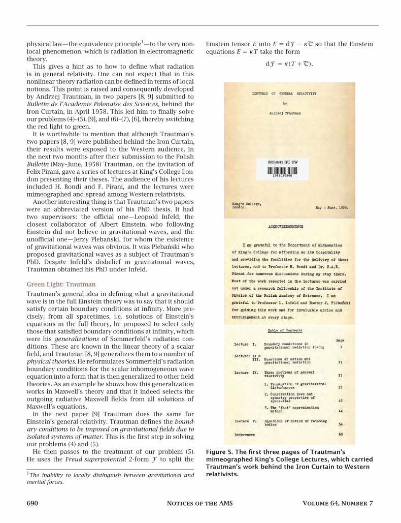
It is worthwhile to mention that although Trautman’stwo papers [8, 9] were published behind the Iron Curtain,their results were exposed to the Western audience. Inthe next two months after their submission to the PolishBulletin (May–June, 1958) Trautman, on the invitation ofFelix Pirani, gave a series of lectures at King’s College Lon-don presenting their theses. The audience of his lecturesincluded H. Bondi and F. Pirani, and the lectures weremimeographed and spread among Western relativists.

Another interesting thing is that Trautman’s two paperswere an abbreviated version of his PhD thesis. It hadtwo supervisors: the official one—Leopold Infeld, theclosest collaborator of Albert Einstein, who followingEinstein did not believe in gravitational waves, and theunofficial one—Jerzy Plebański, for whom the existenceof gravitational waves was obvious. It was Plebański whoproposed gravitational waves as a subject of Trautman’sPhD. Despite Infeld’s disbelief in gravitational waves,Trautman obtained his PhD under Infeld.

Green Light: TrautmanTrautman’s general idea in defining what a gravitationalwave is in the full Einstein theory was to say that it shouldsatisfy certain boundary conditions at infinity. More pre-cisely, from all spacetimes, i.e. solutions of Einstein’sequations in the full theory, he proposed to select onlythose that satisfied boundary conditions at infinity, whichwere his generalizations of Sommerfeld’s radiation con-ditions. These are known in the linear theory of a scalarfield, and Trautman [8, 9] generalizes them to a number ofphysical theories. He reformulates Sommerfeld’s radiationboundary conditions for the scalar inhomogeneous waveequation into a form that is then generalized to other fieldtheories. As an example he shows how this generalizationworks in Maxwell’s theory and that it indeed selects theoutgoing radiative Maxwell fields from all solutions ofMaxwell’s equations.

In the next paper [9] Trautman does the same forEinstein’s general relativity. Trautman defines the bound-ary conditions to be imposed on gravitational fields due toisolated systems of matter. This is the first step in solvingour problems (4) and (5).

He then passes to the treatment of our problem (5).He uses the Freud superpotential 2-form ℱ to split the

1The inability to locally distinguish between gravitational andinertial forces.

Einstein tensor 𝐸 into 𝐸 = dℱ− 𝜅𝔗 so that the Einsteinequations 𝐸 = 𝜅𝑇 take the form

dℱ = 𝜅(𝑇+𝔗).

Figure 5. The first three pages of Trautman’smimeographed King’s College Lectures, which carriedTrautman’s work behind the Iron Curtain to Westernrelativists.


Figure 6. A blackboard discussion betweenTrautman’s two advisors, Jerzy Plebański (left) andLeopold Infeld, at the Institute of Theoretical Physicsof University of Warsaw. Ironically, Trautman got hisPhD on gravitational waves as recommended byPlebański under Infeld, who didn’t believe in them.

Here 𝑇 is the energy-momentum 3-form, and 𝜅 is aconstant related to the gravitational constant 𝐺 and thespeed of light 𝑐 via 𝜅 = 8𝜋𝐺

𝑐4 (in the following we workwith physical units in which 𝑐 = 1).

Since 𝔗 is a 3-form totally determined by the geometry,it is interpreted as the energy-momentum 3-form of puregravity. The closed 3-form 𝑇+𝔗 is then used to definethe 4-momentum 𝑃𝜇(𝜎) of a gravitational field attributedto every space-like hypersurface 𝜎 of a spacetime satis-fying his radiative boundary conditions. He shows that𝑃𝜇(𝜎) is finite and well defined, i.e. that it does not de-pend on the coordinate systems adapted to the chosenboundary conditions. Using his boundary conditions hethen calculates how much of the gravitational energy𝑝𝜇 = 𝑃𝜇(𝜎1) − 𝑃𝜇(𝜎2) contained between the spacelikehypersurfaces 𝜎1 (initial one) and 𝜎2 (final one) escapesto infinity.

Finally, he shows that 𝑝0 is nonnegative, saying thatradiation is present when 𝑝0 > 0.

Taken together, everything we have said so far aboutTrautman’s results, solves our problems (4) and (5): Whatin popular terms is called a gravitational wave in the fullGR theory is a spacetime satisfying Trautman’s boundaryconditions with 𝑝0 > 0; the energy of a gravitational wavecontained between hypersurfaces 𝜎1 and 𝜎2 is given by𝑝0.

Trautman proves only that 𝑝0 ≥ 0. If the inequality weresharp,𝑝0 > 0, thiswould give a proof of the statement thatspacetimes satisfying Trautman’s boundary conditions,or better said, the gravitational waves associated withthem, carry energy. Trautman does not have such a proof.To handle this problem, one can try to find an exampleof an exact solution to the Einstein equations satisfyingTrautman’s boundary conditions, and to show that in thisexample 𝑝0 is strictly greater than zero. This approach

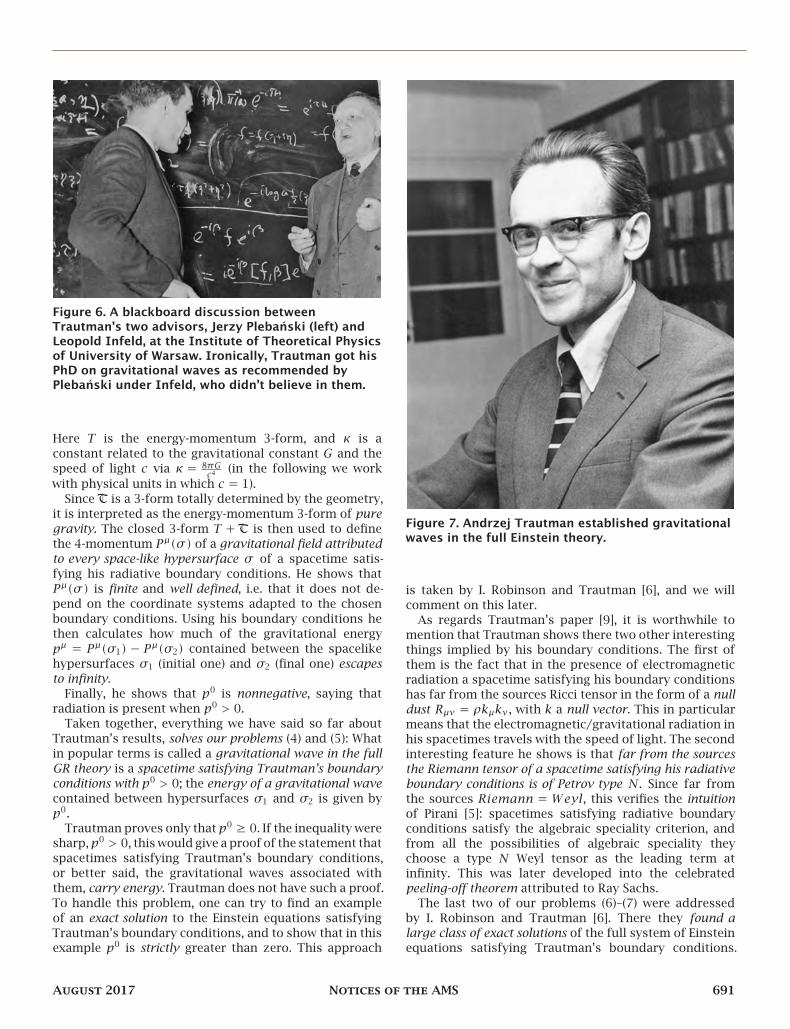
Figure 7. Andrzej Trautman established gravitationalwaves in the full Einstein theory.

is taken by I. Robinson and Trautman [6], and we willcomment on this later.

As regards Trautman’s paper [9], it is worthwhile tomention that Trautman shows there two other interestingthings implied by his boundary conditions. The first ofthem is the fact that in the presence of electromagneticradiation a spacetime satisfying his boundary conditionshas far from the sources Ricci tensor in the form of a nulldust 𝑅𝜇𝜈 = 𝜌𝑘𝜇𝑘𝜈, with 𝑘 a null vector. This in particularmeans that the electromagnetic/gravitational radiation inhis spacetimes travels with the speed of light. The secondinteresting feature he shows is that far from the sourcesthe Riemann tensor of a spacetime satisfying his radiativeboundary conditions is of Petrov type 𝑁. Since far fromthe sources 𝑅𝑖𝑒𝑚𝑎𝑛𝑛 = 𝑊𝑒𝑦𝑙, this verifies the intuitionof Pirani [5]: spacetimes satisfying radiative boundaryconditions satisfy the algebraic speciality criterion, andfrom all the possibilities of algebraic speciality theychoose a type 𝑁 Weyl tensor as the leading term atinfinity. This was later developed into the celebratedpeeling-off theorem attributed to Ray Sachs.

The last two of our problems (6)–(7) were addressedby I. Robinson and Trautman [6]. There they found alarge class of exact solutions of the full system of Einsteinequations satisfying Trautman’s boundary conditions.


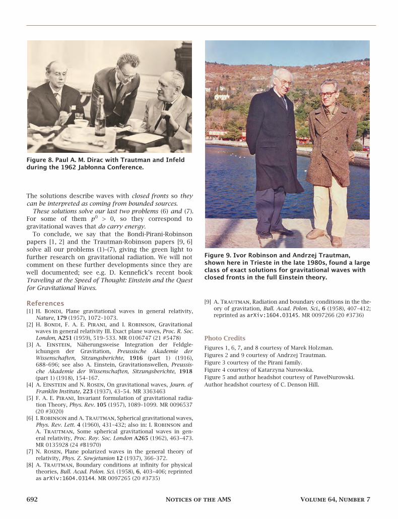
Figure 8. Paul A. M. Dirac with Trautman and Infeldduring the 1962 Jabłonna Conference.

The solutions describe waves with closed fronts so theycan be interpreted as coming from bounded sources.

These solutions solve our last two problems (6) and (7).For some of them 𝑝0 > 0, so they correspond togravitational waves that do carry energy.

To conclude, we say that the Bondi-Pirani-Robinsonpapers [1, 2] and the Trautman-Robinson papers [9, 6]solve all our problems (1)–(7), giving the green light tofurther research on gravitational radiation. We will notcomment on these further developments since they arewell documented; see e.g. D. Kennefick’s recent bookTraveling at the Speed of Thought: Einstein and the Questfor Gravitational Waves.

References[1] H. Bondi, Plane gravitational waves in general relativity,

Nature, 179 (1957), 1072–1073.[2] H. Bondi, F. A. E. Pirani, and I. Robinson, Gravitational

waves in general relativity III. Exact plane waves, Proc. R. Soc.London, A251 (1959), 519–533. MR 0106747 (21 #5478)

[3] A. Einstein, Näherungsweise Integration der Feldgle-ichungen der Gravitation, Preussische Akademie derWissenschaften, Sitzungsberichte, 1916 (part 1) (1916),688–696; see also A. Einstein, Gravitationswellen, Preussis-che Akademie der Wissenschaften, Sitzungsberichte, 1918(part 1) (1918), 154–167.

[4] A. Einstein and N. Rosen, On gravitational waves, Journ. ofFranklin Institute, 223 (1937), 43–54. MR 3363463

[5] F. A. E. Pirani, Invariant formulation of gravitational radia-tion Theory, Phys. Rev. 105 (1957), 1089–1099. MR 0096537(20 #3020)

[6] I. Robinson and A. Trautman, Spherical gravitational waves,Phys. Rev. Lett. 4 (1960), 431–432; also in: I. Robinson andA. Trautman, Some spherical gravitational waves in gen-eral relativity, Proc. Roy. Soc. London A265 (1962), 463–473.MR 0135928 (24 #B1970)

[7] N. Rosen, Plane polarized waves in the general theory ofrelativity, Phys. Z. Sowjetunion 12 (1937), 366–372.

[8] A. Trautman, Boundary conditions at infinity for physicaltheories, Bull. Acad. Polon. Sci. (1958), 6, 403–406; reprintedas arXiv:1604.03144. MR 0097265 (20 #3735)

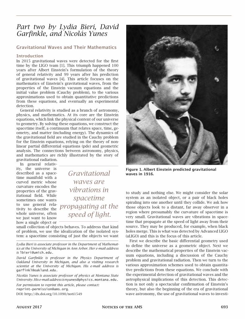
Figure 9. Ivor Robinson and Andrzej Trautman,shown here in Trieste in the late 1980s, found a largeclass of exact solutions for gravitational waves withclosed fronts in the full Einstein theory.

[9] A. Trautman, Radiation and boundary conditions in the the-ory of gravitation, Bull. Acad. Polon. Sci., 6 (1958), 407–412;reprinted as arXiv:1604.03145. MR 0097266 (20 #3736)

Photo CreditsFigures 1, 6, 7, and 8 courtesy of Marek Holzman.Figures 2 and 9 courtesy of Andrzej Trautman.Figure 3 courtesy of the Pirani family.Figure 4 courtesy of Katarzyna Nurowska.Figure 5 and author headshot courtesy of PawełNurowski.Author headshot courtesy of C. Denson Hill.


http://www.ams.org/mathscinet-getitem?mr=0106747





http://www.arXiv.org/abs/1604.03144


Part two by Lydia Bieri, DavidGarfinkle, and Nicolás Yunes

Gravitational Waves and Their Mathematics

IntroductionIn 2015 gravitational waves were detected for the firsttime by the LIGO team [1]. This triumph happened 100years after Albert Einstein’s formulation of the theoryof general relativity and 99 years after his predictionof gravitational waves [4]. This article focuses on themathematics of Einstein’s gravitational waves, from theproperties of the Einstein vacuum equations and theinitial value problem (Cauchy problem), to the variousapproximations used to obtain quantitative predictionsfrom these equations, and eventually an experimentaldetection.

General relativity is studied as a branch of astronomy,physics, and mathematics. At its core are the Einsteinequations, which link the physical content of our universeto geometry. By solving these equations, we construct thespacetime itself, a continuum that relates space, time, ge-ometry, and matter (including energy). The dynamics ofthe gravitational field are studied in the Cauchy problemfor the Einstein equations, relying on the theory of non-linear partial differential equations (pde) and geometricanalysis. The connections between astronomy, physics,and mathematics are richly illustrated by the story ofgravitational radiation.

Gravitationalwaves are

vibrations inspacetime

propagating at thespeed of light.

In general relativ-ity, the universe isdescribed as a space-time manifold with acurved metric whosecurvature encodes theproperties of the grav-itational field. Whilesometimes one wantsto use general rela-tivity to describe thewhole universe, oftenwe just want to knowhow a single object orsmall collection of objects behaves. To address that kindof problem, we use the idealization of the isolated sys-tem: a spacetime consisting of just the objects we want

Lydia Bieri is associate professor in the Department of Mathemat-ics at the University of Michigan in Ann Arbor. Her e-mail addressis [email protected].

David Garfinkle is professor in the Physics Department ofOakland University in Michigan, and also a visiting researchscientist at the University of Michigan. His e-mail address [email protected].

Nicolás Yunes is associate professor of physics at Montana StateUniversity.His e-mail address [email protected].

For permission to reprint this article, please contact:[email protected]: http://dx.doi.org/10.1090/noti1549

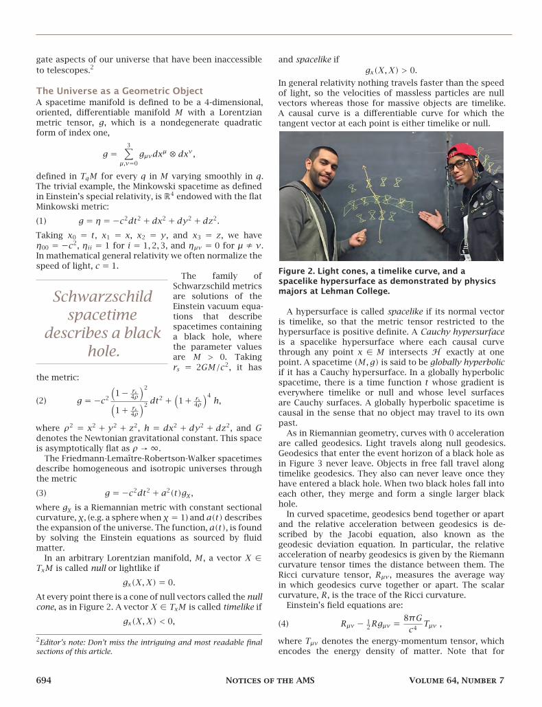
Figure 1. Albert Einstein predicted gravitationalwaves in 1916.

to study and nothing else. We might consider the solarsystem as an isolated object, or a pair of black holesspiraling into one another until they collide. We ask howthose objects look to a distant, far away observer in aregion where presumably the curvature of spacetime isvery small. Gravitational waves are vibrations in space-time that propagate at the speed of light away from theirsource. They may be produced, for example, when blackholes merge. This is what was detected by Advanced LIGO(aLIGO) and this is the focus of this article.

First we describe the basic differential geometry usedto define the universe as a geometric object. Next wedescribe the mathematical properties of the Einstein vac-uum equations, including a discussion of the Cauchyproblem and gravitational radiation. Then we turn to thevarious approximation schemes used to obtain quantita-tive predictions from these equations. We conclude withthe experimental detection of gravitational waves and theastrophysical implications of this detection. This detec-tion is not only a spectacular confirmation of Einstein’stheory, but also the beginning of the era of gravitationalwave astronomy, the use of gravitational waves to investi-


gate aspects of our universe that have been inaccessibleto telescopes.2

The Universe as a Geometric ObjectA spacetime manifold is defined to be a 4-dimensional,oriented, differentiable manifold 𝑀 with a Lorentzianmetric tensor, 𝑔, which is a nondegenerate quadraticform of index one,

𝑔 =3∑

𝜇,𝜈=0𝑔𝜇𝜈𝑑𝑥𝜇 ⊗𝑑𝑥𝜈,

defined in 𝑇𝑞𝑀 for every 𝑞 in 𝑀 varying smoothly in 𝑞.The trivial example, the Minkowski spacetime as definedin Einstein’s special relativity, is ℝ4 endowed with the flatMinkowski metric:(1) 𝑔 = 𝜂 = −𝑐2𝑑𝑡2 +𝑑𝑥2 +𝑑𝑦2 +𝑑𝑧2.Taking 𝑥0 = 𝑡, 𝑥1 = 𝑥, 𝑥2 = 𝑦, and 𝑥3 = 𝑧, we have𝜂00 = −𝑐2, 𝜂𝑖𝑖 = 1 for 𝑖 = 1, 2, 3, and 𝜂𝜇𝜈 = 0 for 𝜇 ≠ 𝜈.In mathematical general relativity we often normalize thespeed of light, 𝑐 = 1.

Schwarzschildspacetime

describes a blackhole.

The family ofSchwarzschild metricsare solutions of theEinstein vacuum equa-tions that describespacetimes containinga black hole, wherethe parameter valuesare 𝑀 > 0. Taking𝑟𝑠 = 2𝐺𝑀/𝑐2, it has

the metric:

(2) 𝑔 = −𝑐2 (1− 𝑟𝑠4𝜌)

2

(1+ 𝑟𝑠4𝜌)

2 𝑑𝑡2 + (1+ 𝑟𝑠4𝜌)

4 ℎ,

where 𝜌2 = 𝑥2 + 𝑦2 + 𝑧2, ℎ = 𝑑𝑥2 + 𝑑𝑦2 + 𝑑𝑧2, and 𝐺denotes the Newtonian gravitational constant. This spaceis asymptotically flat as 𝜌 → ∞.

The Friedmann-Lemaître-Robertson-Walker spacetimesdescribe homogeneous and isotropic universes throughthe metric(3) 𝑔 = −𝑐2𝑑𝑡2 +𝑎2(𝑡)𝑔𝜒,where 𝑔𝜒 is a Riemannian metric with constant sectionalcurvature, 𝜒, (e.g. a sphere when 𝜒 = 1) and 𝑎(𝑡) describesthe expansion of the universe. The function, 𝑎(𝑡), is foundby solving the Einstein equations as sourced by fluidmatter.

In an arbitrary Lorentzian manifold, 𝑀, a vector 𝑋 ∈𝑇𝑥𝑀 is called null or lightlike if

𝑔𝑥(𝑋,𝑋) = 0.At every point there is a cone of null vectors called the nullcone, as in Figure 2. A vector 𝑋 ∈ 𝑇𝑥𝑀 is called timelike if

𝑔𝑥(𝑋,𝑋) < 0,

2Editor’s note: Don’t miss the intriguing and most readable finalsections of this article.

and spacelike if𝑔𝑥(𝑋,𝑋) > 0.

In general relativity nothing travels faster than the speedof light, so the velocities of massless particles are nullvectors whereas those for massive objects are timelike.A causal curve is a differentiable curve for which thetangent vector at each point is either timelike or null.

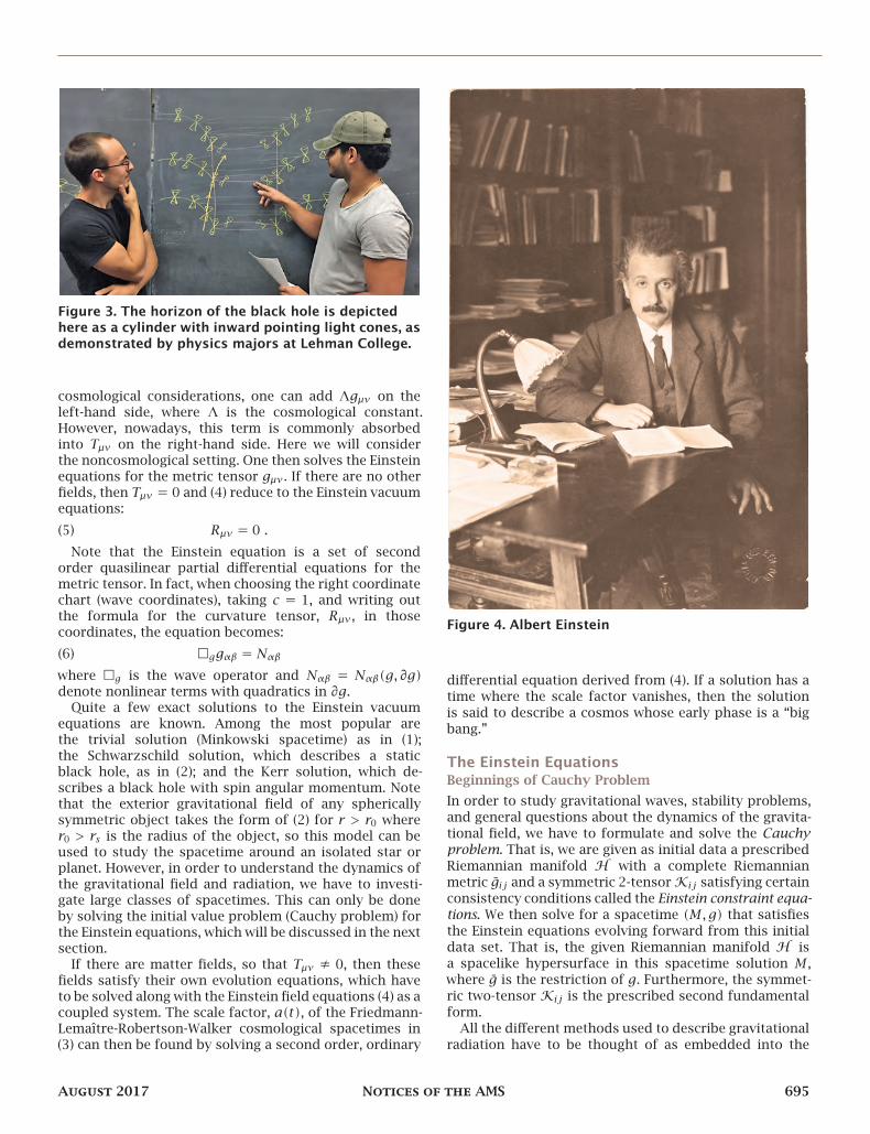
Figure 2. Light cones, a timelike curve, and aspacelike hypersurface as demonstrated by physicsmajors at Lehman College.

A hypersurface is called spacelike if its normal vectoris timelike, so that the metric tensor restricted to thehypersurface is positive definite. A Cauchy hypersurfaceis a spacelike hypersurface where each causal curvethrough any point 𝑥 ∈ 𝑀 intersects ℋ exactly at onepoint. A spacetime (𝑀,𝑔) is said to be globally hyperbolicif it has a Cauchy hypersurface. In a globally hyperbolicspacetime, there is a time function 𝑡 whose gradient iseverywhere timelike or null and whose level surfacesare Cauchy surfaces. A globally hyperbolic spacetime iscausal in the sense that no object may travel to its ownpast.

As in Riemannian geometry, curves with 0 accelerationare called geodesics. Light travels along null geodesics.Geodesics that enter the event horizon of a black hole asin Figure 3 never leave. Objects in free fall travel alongtimelike geodesics. They also can never leave once theyhave entered a black hole. When two black holes fall intoeach other, they merge and form a single larger blackhole.

In curved spacetime, geodesics bend together or apartand the relative acceleration between geodesics is de-scribed by the Jacobi equation, also known as thegeodesic deviation equation. In particular, the relativeacceleration of nearby geodesics is given by the Riemanncurvature tensor times the distance between them. TheRicci curvature tensor, 𝑅𝜇𝜈, measures the average wayin which geodesics curve together or apart. The scalarcurvature, 𝑅, is the trace of the Ricci curvature.

Einstein’s field equations are:

(4) 𝑅𝜇𝜈 − 12𝑅𝑔𝜇𝜈 = 8𝜋𝐺

𝑐4 𝑇𝜇𝜈 ,

where 𝑇𝜇𝜈 denotes the energy-momentum tensor, whichencodes the energy density of matter. Note that for


Figure 3. The horizon of the black hole is depictedhere as a cylinder with inward pointing light cones, asdemonstrated by physics majors at Lehman College.

cosmological considerations, one can add Λ𝑔𝜇𝜈 on theleft-hand side, where Λ is the cosmological constant.However, nowadays, this term is commonly absorbedinto 𝑇𝜇𝜈 on the right-hand side. Here we will considerthe noncosmological setting. One then solves the Einsteinequations for the metric tensor 𝑔𝜇𝜈. If there are no otherfields, then 𝑇𝜇𝜈 = 0 and (4) reduce to the Einstein vacuumequations:(5) 𝑅𝜇𝜈 = 0 .

Note that the Einstein equation is a set of secondorder quasilinear partial differential equations for themetric tensor. In fact, when choosing the right coordinatechart (wave coordinates), taking 𝑐 = 1, and writing outthe formula for the curvature tensor, 𝑅𝜇𝜈, in thosecoordinates, the equation becomes:(6) □𝑔𝑔𝛼𝛽 = 𝑁𝛼𝛽

where □𝑔 is the wave operator and 𝑁𝛼𝛽 = 𝑁𝛼𝛽(𝑔, 𝜕𝑔)denote nonlinear terms with quadratics in 𝜕𝑔.

Quite a few exact solutions to the Einstein vacuumequations are known. Among the most popular arethe trivial solution (Minkowski spacetime) as in (1);the Schwarzschild solution, which describes a staticblack hole, as in (2); and the Kerr solution, which de-scribes a black hole with spin angular momentum. Notethat the exterior gravitational field of any sphericallysymmetric object takes the form of (2) for 𝑟 > 𝑟0 where𝑟0 > 𝑟𝑠 is the radius of the object, so this model can beused to study the spacetime around an isolated star orplanet. However, in order to understand the dynamics ofthe gravitational field and radiation, we have to investi-gate large classes of spacetimes. This can only be doneby solving the initial value problem (Cauchy problem) forthe Einstein equations, which will be discussed in the nextsection.

If there are matter fields, so that 𝑇𝜇𝜈 ≠ 0, then thesefields satisfy their own evolution equations, which haveto be solved along with the Einstein field equations (4) as acoupled system. The scale factor, 𝑎(𝑡), of the Friedmann-Lemaître-Robertson-Walker cosmological spacetimes in(3) can then be found by solving a second order, ordinary

Figure 4. Albert Einstein

differential equation derived from (4). If a solution has atime where the scale factor vanishes, then the solutionis said to describe a cosmos whose early phase is a “bigbang.”

The Einstein EquationsBeginnings of Cauchy ProblemIn order to study gravitational waves, stability problems,and general questions about the dynamics of the gravita-tional field, we have to formulate and solve the Cauchyproblem. That is, we are given as initial data a prescribedRiemannian manifold ℋ with a complete Riemannianmetric 𝑔𝑖𝑗 and a symmetric 2-tensor𝒦𝑖𝑗 satisfying certainconsistency conditions called the Einstein constraint equa-tions. We then solve for a spacetime (𝑀,𝑔) that satisfiesthe Einstein equations evolving forward from this initialdata set. That is, the given Riemannian manifold ℋ isa spacelike hypersurface in this spacetime solution 𝑀,where 𝑔 is the restriction of 𝑔. Furthermore, the symmet-ric two-tensor 𝒦𝑖𝑗 is the prescribed second fundamentalform.

All the different methods used to describe gravitationalradiation have to be thought of as embedded into the


aim of solving the Cauchy problem. We solve the Cauchyproblem by methods of analysis and geometry. However,for situations where the geometric-analytic techniquesare not (yet) at hand, one uses approximation methodsand numerical algorithms. The goal of the latter methodsis to produce approximations to solutions of the Cauchyproblem for the Einstein equations.

In order to derive the gravitational waves from bi-nary black hole mergers, binary neutron star mergers,or core-collapse supernovae, we describe these systemsby asymptotically flat spacetimes. These are solutions ofthe Einstein equations that at infinity tend to Minkowskispace with a metric as in (1). Schwarzschild space is a sim-ple example of such an isolated system containing only asingle stationary black hole (2). There is a huge literatureabout specific fall-off rates, which we will not describehere. The null asymptotics of these spacetimes contain in-formation on gravitational radiation (gravitational waves)out to infinity.

Recall that the Einstein vacuum equations (5) are a sys-tem of ten quasilinear, partial differential equations thatcan be put into hyperbolic form.However, with the Bianchiidentity imposing four constraints, the Einstein vacuumsystem (5) constitutes only six independent equations forthe ten unknowns of the metric 𝑔𝜇𝜈. This corresponds tothe general covariance of the Einstein equations. In fact,uniqueness of solutions to these equations holds up toequivalence under diffeomorphisms. We have just founda core feature of general relativity. This mathematicalfact also means that physical laws do not depend on thecoordinates used to describe a particular process.

The Einstein equations split into a set of evolutionequations and a set of constraint equations. As above, 𝑡denotes the time coordinate whereas indices 𝑖, 𝑗 = 1,… ,3refer to spatial coordinates. Taking 𝑐 = 1, the evolutionequations read:

𝜕 𝑔𝑖𝑗𝜕𝑡 = −2Φ𝒦𝑖𝑗 +ℒ𝑋 𝑔𝑖𝑗,(7)

𝜕𝒦𝑖𝑗𝜕𝑡 = −∇𝑖∇𝑗Φ+ℒ𝑋𝒦𝑖𝑗

+ (��𝑖𝑗 + 𝒦𝑖𝑗 𝑡𝑟𝒦 − 2𝒦𝑖𝑚𝒦𝑚𝑗 )Φ(8)

Here 𝒦𝑖𝑗 is the extrinsic curvature of the 𝑡 = 𝑐𝑜𝑛𝑠𝑡.surfaceℋ as above. The lapseΦ and shift𝑋 are essentiallythe 𝑔𝑡𝑡 and 𝑔𝑡𝑖 components of the metric, and are given by𝑇 = Φ𝑛+𝑋 where 𝑇 is the evolution vector field 𝜕/𝜕𝑡 and𝑛 is the unit normal to the constant time hypersurface.∇𝑖 is the spatial covariant derivative and ℒ is the Liederivative. However, the initial data ( 𝑔𝑖𝑗,𝒦𝑖𝑗) cannotbe chosen freely: the remaining four Einstein vacuumequations become the following constraint equations:

∇𝑖𝒦𝑖𝑗 − ∇𝑗 𝑡𝑟𝒦 = 0,(9)�� + (𝑡𝑟𝒦)2 − |𝒦|2 = 0.(10)

An initial data set is a 3-dimensional manifold ℋ witha complete Riemannian metric 𝑔𝑖𝑗 and a symmetric 2-tensor 𝒦𝑖𝑗 satisfying the constraint equations ((9) and(10)). We will evolve an asymptotically flat initial data set(ℋ, 𝑔𝑖𝑗,𝒦𝑖𝑗), that outside a sufficiently large compact set𝒟, ℋ\𝒟 is diffeomorphic to the complement of a closed

ball in ℝ3 and admits a system of coordinates where𝑔𝑖𝑗 → 𝛿𝑖𝑗 and 𝒦𝑖𝑗 → 0 sufficiently fast.It took a long time before the Cauchy problem for the

Einstein equations was formulated correctly and under-stood. Geometry and pde theory were not as developedas they are today, and the pioneers of general relativityhad to struggle with problems that have elegant solu-tions nowadays. The beauty and challenges of generalrelativity attracted many mathematicians, as for instanceD. Hilbert or H. Weyl, to work on general relativity’sfundamental questions. Weyl in 1923 talked about a“causally connected” world, which hints at issues thatthe domain of dependence theorem much later wouldsolve. G. Darmois in the 1920s studied the analytic case,which is not physical but a step in the right direction. Herecognized that the analyticity hypothesis is physicallyunsatisfactory, because it hides the propagation proper-ties of the gravitational field. Without going into details,important work followed by K. Stellmacher, K. Friedrichs,T. de Donder, and C. Lanczos. The latter two introducedwave coordinates, which Darmois later used. In 1939, A.Lichnerowicz extended Darmois’ work. He also suggestedthe extension of the 3 + 1 decomposition with nonzeroshift to his student Yvonne Choquet-Bruhat, which shecarried out.

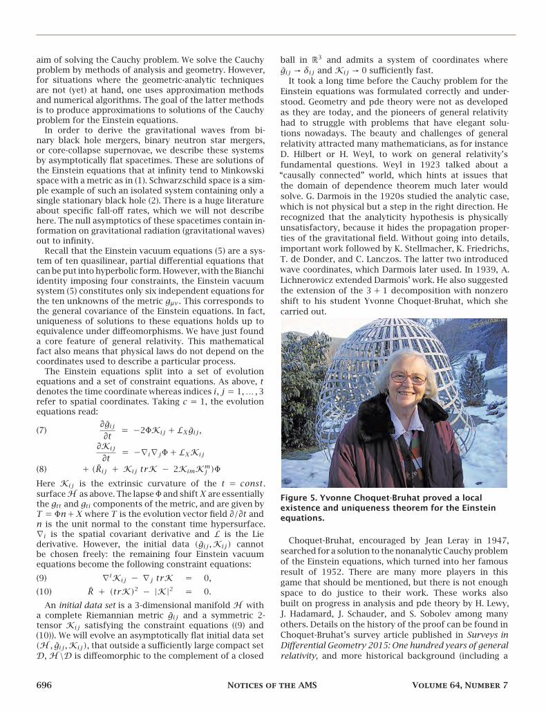
Figure 5. Yvonne Choquet-Bruhat proved a localexistence and uniqueness theorem for the Einsteinequations.

Choquet-Bruhat, encouraged by Jean Leray in 1947,searched for a solution to the nonanalytic Cauchyproblemof the Einstein equations, which turned into her famousresult of 1952. There are many more players in thisgame that should be mentioned, but there is not enoughspace to do justice to their work. These works alsobuilt on progress in analysis and pde theory by H. Lewy,J. Hadamard, J. Schauder, and S. Sobolev among manyothers. Details on the history of the proof can be found inChoquet-Bruhat’s survey article published in Surveys inDifferential Geometry 2015: One hundred years of generalrelativity, and more historical background (including a


discussion between Choquet-Bruhat and Einstein) is givenin Choquet-Bruhat’s forthcoming autobiography.

In 1952 Choquet-Bruhat [2] proved a local existence anduniqueness theorem for the Einstein equations, and in1969 Choquet-Bruhat and R. Geroch [3] proved the globalexistence of a unique maximal future development forevery given initial data set.

Theorem 1 (Choquet-Bruhat, 1952). Let (ℋ, 𝑔,𝒦) be aninitial data set satisfying the vacuum constraint equations.Then there exists a spacetime (𝑀,𝑔) satisfying the Einsteinvacuum equations with ℋ ↪ 𝑀 being a spacelike surfacewith induced metric 𝑔 and second fundamental form 𝒦.

This was proven by finding a useful coordinate system,called wave coordinates, in which Einstein’s vacuumequations appear clearly as a hyperbolic system of partialdifferential equations. The pioneering result by Choquet-Bruhat was improved by Dionne (1962), Fisher-Marsden(1970), and Hughes-Kato-Marsden (1977) using the energymethod.

Global Cauchy ProblemChoquet-Bruhat’s local theorem of 1952 was a break-through and has since been fundamental for furtherinvestigations of the Cauchy problem. Once we havelocal solutions of the Einstein equations, do they existfor all time, or do they form singularities? And of whattype would the latter be? In 1969 Choquet-Bruhat andGeroch proved there exists a unique, globally hyperbolic,maximal spacetime (𝑀,𝑔) satisfying the Einstein vacuumequations with ℋ ↪ 𝑀 being a Cauchy surface withinduced metric 𝑔 and second fundamental form 𝒦. Thisunique solution is called the maximal future developmentof the initial data set.

However, there is no information about the behaviorof the solution. Will singularities occur or will it becomplete? One would expect that sufficiently small initialdata evolves forever without producing any singularities,whereas sufficiently large data evolves to form spacetimesingularities such as black holes. From a mathematicalpoint of view the question is whether theorems canbe proven that establish this behavior. A breakthroughoccurred in 2008 with Christodoulou’s proof, buildingon an earlier result due to Penrose, that black holesingularities form in the Cauchy development of initialdata, which do not contain any singularities, providedthat the incoming energy per unit solid angle in eachdirection in a suitably small time interval is sufficientlylarge. This means that a black hole forms through thefocussingofgravitationalwaves.This resulthas sincebeengeneralized by various authors, and the main methodshave been applied to other nonlinear pdes.

The next burning question to ask is whether there isany asymptotically flat (and nontrivial) initial data withcomplete maximal development. This can be thought ofas a question about the global stability of Minkowskispace. In their celebrated work of 1993, D. Christodoulouand S. Klainerman proved the following result, which herewe state in a very general way. The details are intricate

and the smallness assumptions are stated for weightedSobolev norms of the geometric quantities.

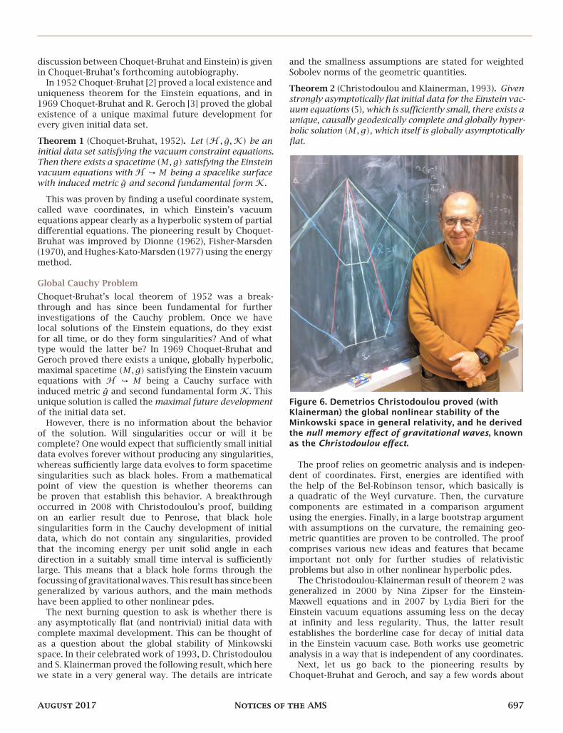
Theorem 2 (Christodoulou and Klainerman, 1993). Givenstrongly asymptotically flat initial data for the Einstein vac-uum equations (5), which is sufficiently small, there exists aunique, causally geodesically complete and globally hyper-bolic solution (𝑀,𝑔), which itself is globally asymptoticallyflat.

Figure 6. Demetrios Christodoulou proved (withKlainerman) the global nonlinear stability of theMinkowski space in general relativity, and he derivedthe null memory effect of gravitational waves, knownas the Christodoulou effect.

The proof relies on geometric analysis and is indepen-dent of coordinates. First, energies are identified withthe help of the Bel-Robinson tensor, which basically isa quadratic of the Weyl curvature. Then, the curvaturecomponents are estimated in a comparison argumentusing the energies. Finally, in a large bootstrap argumentwith assumptions on the curvature, the remaining geo-metric quantities are proven to be controlled. The proofcomprises various new ideas and features that becameimportant not only for further studies of relativisticproblems but also in other nonlinear hyperbolic pdes.

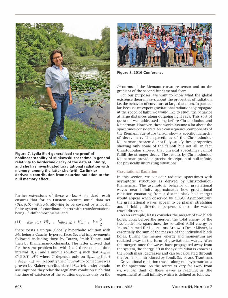
The Christodoulou-Klainerman result of theorem 2 wasgeneralized in 2000 by Nina Zipser for the Einstein-Maxwell equations and in 2007 by Lydia Bieri for theEinstein vacuum equations assuming less on the decayat infinity and less regularity. Thus, the latter resultestablishes the borderline case for decay of initial datain the Einstein vacuum case. Both works use geometricanalysis in a way that is independent of any coordinates.

Next, let us go back to the pioneering results byChoquet-Bruhat and Geroch, and say a few words about


Figure 7. Lydia Bieri generalized the proof ofnonlinear stability of Minkowski spacetime in generalrelativity to borderline decay of the data at infinity,and she has investigated gravitational radiation withmemory; among the latter she (with Garfinkle)derived a contribution from neutrino radiation to thenull memory effect.

further extensions of these works. A standard resultensures that for an Einstein vacuum initial data set(ℋ0, 𝑔,𝒦) with ℋ0 allowing to be covered by a locallyfinite system of coordinate charts with transformationsbeing 𝐶1-diffeomorphisms, and

(11) 𝑔𝑚𝑛|ℋ0 ∈ 𝐻𝑘𝑙𝑜𝑐 , 𝜕0𝑔𝑚𝑛|ℋ0 ∈ 𝐻𝑘−1

𝑙𝑜𝑐 , 𝑘 > 52 ,

there exists a unique globally hyperbolic solution withℋ0 being a Cauchy hypersurface. Several improvementsfollowed, including those by Tataru, Smith-Tataru, andthen by Klainerman-Rodnianski. The latter proved thatfor the same problem but with 𝑘 > 2 there exists a timeinterval [0,𝑇] and a unique solution 𝑔 such that 𝑔𝑚𝑛 ∈𝐶0([0,𝑇],𝐻𝑘) where 𝑇 depends only on ||𝑔𝑚𝑛|ℋ0||𝐻𝑘 +||𝜕0𝑔𝑚𝑛|ℋ0||𝐻𝑘−1 . Recently the 𝐿2 curvature conjecture wasproven by Klainerman-Rodnianski-Szeftel: under certainassumptions they relax the regularity condition such thatthe time of existence of the solution depends only on the

Figure 8. 2016 Conference

𝐿2-norms of the Riemann curvature tensor and on thegradient of the second fundamental form.

For our purposes, we want to know what the globalexistence theorem says about the properties of radiation,i.e. the behavior of curvature at large distances. In particu-lar, becausewe expect gravitational radiation to propagateat the speed of light, we would like to study the behaviorat large distances along outgoing light rays. This sort ofquestion was addressed long before Christodoulou andKainerman. However, these works assume a lot about thespacetimes considered. As a consequence, components ofthe Riemann curvature tensor show a specific hierarchyof decay in 𝑟. The spacetimes of the Christodoulou-Klainerman theorem do not fully satisfy these properties,showing only some of the fall-off but not all. In fact,Christodoulou showed that physical spacetimes cannotfulfill the stronger decay. The results by Christodoulou-Klainerman provide a precise description of null infinityfor physically interesting situations.

Gravitational RadiationIn this section, we consider radiative spacetimes withasymptotic structures as derived by Christodoulou-Klainerman. The asymptotic behavior of gravitationalwaves near infinity approximates how gravitationalradiation emanating from a distant black hole mergerwould appear when observed by aLIGO. Asymptoticallythe gravitational waves appear to be planar, stretchingand shrinking directions perpendicular to the wave’stravel direction.

As an example, let us consider the merger of two blackholes. Long before the merger, the total energy of thetwo-black-hole spacetime, the so-called ADM energy or“mass,” named for its creators Arnowitt-Deser-Misner, isessentially the sum of the masses of the individual blackholes. During the merger, energy and momentum areradiated away in the form of gravitational waves. Afterthe merger, once the waves have propagated away fromthe system, the energy left in the system, what is known asthe Bondi mass, decreases and can be calculated throughthe formalism introduced by Bondi, Sachs, and Trautman.

Gravitational radiation travels along null hypersurfacesin the spacetime. As the source is very far away fromus, we can think of these waves as reaching us (theexperiment) at null infinity, which is defined as follows.


Figure 9. Gravitational waves demonstrated by LuisAnchordoqui of Lehman College. Here the horizon ofthe merging black holes is depicted in red and thenthe waves propagate at the speed of light towardsEarth located at null infinity.

Definition 1. Future null infinity ℐ+ is defined to bethe endpoints of all future-directed null geodesics alongwhich 𝑟 → ∞. It has the topology of ℝ × 𝕊2 with thefunction 𝑢 taking values in ℝ.

A null hypersurface 𝒞𝑢 intersects ℐ+ at infinity in a2-sphere. Toeach𝒞𝑢 atnull infinity is assignedaTrautman-Bondi mass𝑀(𝑢), as introduced by Bondi, Trautman, andSachs in the middle of the last century. This quantitymeasures the amount of mass that remains in an isolatedgravitational system at a given retarded time, i.e. theTrautman-Bondi mass measures the remaining mass afterradiation through ℐ+ up to𝑢. The Bondimass-loss formulareads for 𝑢1 ≤ 𝑢2

(12) 𝑀(𝑢2) = 𝑀(𝑢1) − 𝐶∫𝑢2

𝑢1

∫𝑆2

|Ξ|2 𝑑𝜇∘𝛾𝑑𝑢

with |Ξ|2 being the norm of the shear tensor at ℐ+ and 𝑑𝜇∘𝛾

the canonical measure on 𝑆2. If other fields are present,like electromagnetic fields, then the formula containsa corresponding term for that field. In the situationsconsidered here, it has been proven that lim𝑢→−∞ 𝑀(𝑢) =𝑀𝐴𝐷𝑀.

The effects of gravitational waves on neighboringgeodesics are encoded in the Jacobi equation. Thisvery fact is at the heart of the detection by aLIGOand is discussed in the section entitled GravitationalWave Experiment. From this, we derive a formula for thedisplacement of testmasses, while the wave packet is trav-eling through the apparatus. This is what was measuredby the aLIGO detectors.

Now, there is more to the story. From the analysis ofthe spacetime at ℐ+ one can prove that the test masseswill go to rest after the gravitational wave has passed,meaning that the geodesics will not be deviated anymore.However, will the test masses be at the “same” position asbefore the wave train passed or will they be dislocated?In mathematical language, will the spacetime geometryhave changed permanently? If so, then this is called thememory effect of gravitational waves. This effect was first

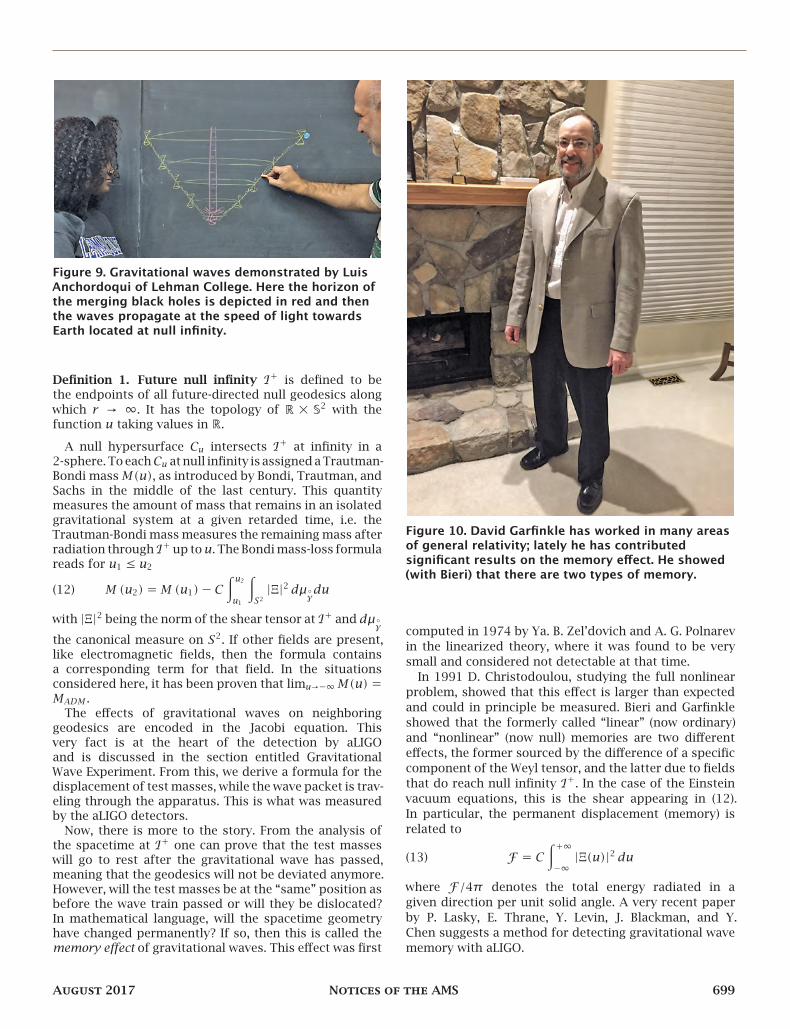
Figure 10. David Garfinkle has worked in many areasof general relativity; lately he has contributedsignificant results on the memory effect. He showed(with Bieri) that there are two types of memory.

computed in 1974 by Ya. B. Zel’dovich and A. G. Polnarevin the linearized theory, where it was found to be verysmall and considered not detectable at that time.

In 1991 D. Christodoulou, studying the full nonlinearproblem, showed that this effect is larger than expectedand could in principle be measured. Bieri and Garfinkleshowed that the formerly called “linear” (now ordinary)and “nonlinear” (now null) memories are two differenteffects, the former sourced by the difference of a specificcomponent of the Weyl tensor, and the latter due to fieldsthat do reach null infinity ℐ+. In the case of the Einsteinvacuum equations, this is the shear appearing in (12).In particular, the permanent displacement (memory) isrelated to

(13) ℱ = 𝐶∫+∞

−∞|Ξ(𝑢)|2 𝑑𝑢

where ℱ/4𝜋 denotes the total energy radiated in agiven direction per unit solid angle. A very recent paperby P. Lasky, E. Thrane, Y. Levin, J. Blackman, and Y.Chen suggests a method for detecting gravitational wavememory with aLIGO.


Approximation MethodsTo compare gravitational wave experimental data to thepredictions of the theory, one needs a calculation ofthe predictions of the theory. It is not enough to knowthat solutions of the Einstein field equations exist; rather,one needs quantitative solutions of those equations toat least the accuracy needed to compare to experiments.In addition, sometimes the gravitational wave signal isso weak that to keep it from being overwhelmed bynoise one must use the technique of matched filtering inwhich one looks for matches between the signal and aset of templates of possible expected waveforms. Thesequantitative solutions are provided by a set of overlappingapproximation techniques, and by numerical simulations.We will discuss the approximation techniques in thissection and the numerical methods in the section entitledMathematics and Numerics.

Linearized Theory and Gravitational Waves. Since gravi-tational waves become weaker as they propagate awayfrom their sources, one might hope to neglect the nonlin-earities of the Einstein field equations and focus insteadon the linearized equations, which are easier to workwith. One may hope that these equations would providean approximate description of the gravitational radiationfor much of its propagation and for its interaction withthe detector. In linearized gravity, one then writes thespacetime metric as(14) 𝑔𝜇𝜈 = 𝜂𝜇𝜈 +ℎ𝜇𝜈

where 𝜂𝜇𝜈 is the Minkowski metric as in (1) and ℎ𝜇𝜈is assumed to be small. One then keeps terms in theEinstein field equations only to linear order in ℎ𝜇𝜈. Thecoordinate invariance of general relativity gives rise towhat is called gauge invariance in linearized gravity. Inparticular, consider any quantity 𝐹 written as 𝐹 = 𝐹+𝛿𝐹where 𝐹 is the value of the quantity in the background and𝛿𝐹 is the first order perturbation of that quantity. Thenfor an infinitesimal diffeomorphism along the vector field𝜉, the quantity 𝛿𝐹 changes by

𝛿𝐹 → 𝛿𝐹+ℒ𝜉 𝐹,where recall that ℒ stands for the Lie derivative. Recallalso that harmonic coordinatesmade the Einstein vacuumequations look like the wave equation in (6). We wouldlike to do something similar in linearized gravity. To thisend we choose 𝜉 to impose the Lorenz gauge condition(not Lorentz!)

𝜕𝜇ℎ𝜇𝜈 = 0,where

ℎ𝜇𝜈 = ℎ𝜇𝜈 − (1/2)𝜂𝜇𝜈ℎ.The linearized Einstein field equations then become(15) □ℎ𝜇𝜈 = −16𝜋𝐺𝑇𝜇𝜈,where □ is the wave operator in Minkowski spacetime.

In a vacuum one can use the remaining freedom tochoose 𝜉 to impose the conditions that ℎ𝜇𝜈 has onlyspatial components and is trace-free, while remaining inLorenz gauge. This refinement of the Lorenz gauge iscalled the TT gauge, since it guarantees that the only

two propagating degrees of freedom of the metric pertur-bation are transverse 𝜕𝑖ℎ𝑖𝑗 = 0 and (spatially) traceless𝜂𝑖𝑗ℎ𝑖𝑗 = 0. The metric in TT gauge has a direct physicalinterpretation given by the following formula for thelinearized Riemannian curvature tensor

(16) 𝑅𝑖𝑡𝑗𝑡 = −12ℎ

𝑇𝑇𝑖𝑗 ,

which sources the geodesic deviation equation, and thusencapsulates how matter behaves in the presence ofgravitational waves. Combining Eq. (16) and the Jacobiequation, one can compute the change indistance betweentwo test masses in free fall:

△𝑑𝑖(𝑡) = 12ℎ

𝑇𝑇𝑖𝑗 (𝑡)𝑑𝑗

0

where 𝑑𝑗0 is the initial distance between the test masses.

The TT nature of gravitational wave perturbationsallows us to immediately infer that they only have twopolarizations. Consider a wave traveling along the 𝑧-direction, such that ℎ𝑇𝑇

𝑖𝑗 (𝑡 − 𝑧) is a solution of □ℎ𝑇𝑇𝑖𝑗 = 0.

The Lorenz condition, the assumption that the metricperturbation vanishes for large 𝑟, the trace-free condition,and symmetries imply that there are only two independentpropagating degrees of freedom:

ℎ+(𝑡 − 𝑧) = ℎ𝑇𝑇𝑥𝑥 = −ℎ𝑇𝑇

𝑦𝑦

andℎ×(𝑡 − 𝑧) = ℎ𝑇𝑇

𝑥𝑦 = ℎ𝑇𝑇𝑦𝑥 .

The ℎ+ gravitational wave stretches the 𝑥 direction inspace while it squeezes the 𝑦 direction, and vice-versa.The interferometer used to detect gravitational waves hastwo long perpendicular arms that measure this distortion.Therefore, one must approximate these displacements inorder to predict what the interferometer will see undervarious scenarios.

The Post-Newtonian ApproximationThe post-Newtonian (PN) approximation for gravitationalwaves extends the linearized study presented above tohigher orders in the metric perturbation, while alsoassuming that the bodies generating the gravitationalfield move slowly compared to the speed of light. ThePN approach was developed by Einstein, Infeld, Hoffman,Damour, Deruelle, Blanchet, Will, Schaefer, and manyothers. In theharmonic gauge𝜕𝛼(√−𝑔𝑔𝛼𝛽) = 0 commonlyemployed in PN theory, the expanded equations take theform

(17) □ℎ𝛼𝛽 = −16𝜋𝐺𝑐4 𝜏𝛼𝛽 ,

where □ is the wave operator and𝜏𝛼𝛽 = −(𝑔)𝑇𝛼𝛽 + (16𝜋)−1𝑁𝛼𝛽,

with 𝑁𝛼𝛽 composed of quadratic forms of the metricperturbation.

These expanded equations can then be solved orderby order in the perturbation through Green functionmethods, where the integral is over the past lightconeof Minkowski space for 𝑥 ∈ 𝑀. When working at suf-ficiently high PN order, the resulting integrals can be


formally divergent, but these pathologies can be by-passed or cured through asymptotic matching methods(as inWill’s method of the direct integration of the relaxedEinstein equations) or through regularization techniques(as in Blanchet and Damour’s Hadamard and dimensionalregularization approach). All approaches to cure thesepathologies have been shown to lead to exactly the sameend result for the metric perturbation.

The metric perturbation is solved for order by order,where at each order one uses the previously calculatedinformation in the expression for 𝑁𝛼𝛽 and also to findthe motion of the matter sources, thus leading to animproved expression for 𝑇𝛼𝛽 at each order. In particular,the emission of gravitational waves by a binary systemcauses a change in the period of that system, and thischange was used by Hulse and Taylor to indirectly detectgravitational waves through their observations of thebinary pulsar. In this way, the PN iterative procedureprovides a perturbative approximation to the solution tothe Einstein equations to a given order in the feebleness ofthe gravitational interaction and the speed of the bodies.

Little work has gone into studying the mathematicalproperties of the resulting perturbative series. Clearly,the PN approximation should not be valid when the speedof the bodies becomes comparable to the speed of lightor when the objects described are black holes or neutronstars with significant self-gravity. Damour, however, hasshown that the latter can still be described by the PNapproximation up to a given order in perturbation theory.Moreover, recent numerical simulations of the merger ofbinary black holes and neutron stars have shown thatthe PN approximation is accurate even quite late in theinspiral, when the objects are moving at close to a thirdof the speed of light.

Resummations of the PN ApproximationThe accuracy of the approximate solutions can beimprovedbyapplying resummation techniques: the rewrit-ing of the perturbative expansion in a new form (e.g. aChebyshevdecomposition or a Padé series) thatmakesuseof some physical feature one knows should be present inthe exact solution. For example, one may know (throughsymmetry arguments or by taking certain limits) thatsome exact result contains a first-order pole at a certainspacetime position, so one could rewrite the approximatesolution as a Padé approximant that makes this poleexplicit.

A particular resummation of the PN approximation thathas been highly successful at approximating numericalsolutions is the effective one-body approach. Recall that inNewtonian gravity, themotion ofmasses𝑚1 and𝑚2 undertheir mutual gravitational attraction is mathematicallyequivalent to the motion of a single mass 𝜇 in thegravitational field of a stationary mass 𝑀, where 𝑀 =𝑚1 + 𝑚2 and 𝜇 = (𝑚1𝑚2)/𝑀. The effective one bodyapproach similarly attempts to recast the motion of twoblack holes under their mutual gravitational attraction asthe motion of a single object in a given spacetime metric.

More precisely, one recasts the two-body problem ontotheproblemof an effective body thatmoves onan effective

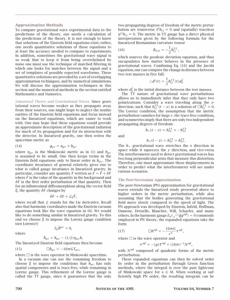
Figure 11. Numerical simulation of the late inspiral ofan unequal-mass, black hole binary. Even late in theinspiral, the PN approximation for gravitationalwaves remains accurate.

external metric through an energy map and a canonicaltransformation. The dynamics of the effective body arethen described through a (conservative) improved Hamil-tonian and a (dissipative) improved radiation-reactionforce. The improved Hamiltonian is resummed throughtwo sets of square-roots of PN series, in such a way soas to reproduce the standard PN Hamiltonian when Tay-lor expanded about weak-field and slow-velocities. Theimproved radiation-reaction force is constructed fromquadratic first-derivatives of the gravitational waves,which in turn are product-resummed using the Hamil-tonian (from knowledge of the extreme mass-ratio limitof the PN expansion) and a field-theory resummation ofcertain tail-effects.

Once the two-body problem has been reformulated,the Hamilton equations associated with the improvedHamiltonian and radiation-reaction force are solved nu-merically, a significantly easier problem than solving thefull Einstein equations. This resummation, however, is notenough because the improved Hamiltonian and radiation-reaction force are built from finite PN expansions. Thevery late inspiral behavior of the solution can be cor-rected by adding calibration coefficients (consistent withPN terms not yet calculated) to the Hamiltonian and theradiation-reaction force, which are then determined byfitting to a set of full, numerical relativity simulations.

The calibrated effective-one-body waveforms describedabove are incredibly accurate representations of the


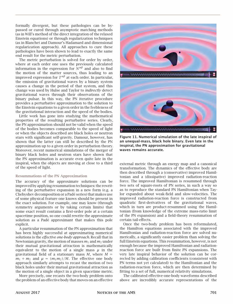
Figure 12. Numerical simulation of the merger of anunequal-mass, black hole binary. Theeffective-one-body approximation remains highlyaccurate almost up to the moment when the blackholes horizons touch, when full numericalsimulations are required.

gravitational waves emitted in the inspiral of compactobjects, up to the moment when the black holes merge.They become accurate after the merger by adding oninformation from black hole perturbation theory that wedescribe next.

Perturbations About a Black Hole BackgroundAfter the black holes merge, they form a single distortedblack hole that sheds its distortions by emitting gravita-tional waves and eventually settling down to a Kerr blackhole. This “ringdown” phase is described using perturba-tion theory with the Einstein vacuum equations linearizedaround a Kerr black hole background. Teukolsky showedhow to obtain a wave type equation for these perturbedWeyl tensor components from the Einstein vacuum equa-tions. The result of the Teukolsky method is that thedistortions can be expanded in modes, each of which hasa characteristic frequency and exponential decay time.The ringdown is well approximated by the most slowlydecaying of these modes. This ringdown waveform can bestitched to the effective-one-body inspiral waveforms toobtain a complete description of the gravitational wavesemitted in the coalescence of black holes.

Mathematics and NumericsIn numerical relativity, one creates simulations of theEinstein field equations using a computer. This is neededwhen no other method will work, in particular whengravity is very strong and highly dynamical (as it is whentwo black holes merge).

The Einstein field equations, like most of the equa-tions of physics, are differential equations, and the moststraightforward of the techniques for simulating differ-ential equations are finite difference equations. In theone-dimensional setting, one approximates a function𝑓(𝑥) by its values on equally spaced points

𝑓𝑖 = 𝑓(𝑖𝛿) for 𝑖 ∈ ℕ.One then approximates derivatives of 𝑓 using differences

𝑓′ ≈ (𝑓𝑖+1 − 𝑓𝑖−1)/(2𝛿)and

𝑓′′(𝑖) ≈ (𝑓𝑖+1 + 𝑓𝑖−1 −2𝑓𝑖)/𝛿2.For any pde with an initial value formulation one replacesthe fields by their values on a spacetime lattice, andthe field equations by finite difference equations thatdetermine the fields at time step 𝑛+ 1 from their valuesat time step 𝑛. Thus the Einstein vacuum equationsare written as difference equations where the step 0information is the initial data set.

One then writes a computer program that implementsthis determination and runs the program. Sounds simple,right? So what could go wrong? Quite a lot, actually. Itis best to think of the solution of the finite differenceequation as something that is supposed to converge toa solution of the differential equation in the limit as thestep size 𝛿 between the lattice points goes to zero. But itis entirely possible that the solution does not converge toanything at all in this limit. In particular, the coordinateinvariance of general relativity allows one to express theEinstein field equations in many different forms, some ofwhich are not strongly hyperbolic. Computer simulationsof these forms of the Einstein field equations generallydo not converge.

Another problem has to do with the constraint equa-tions. Recall that initial data have to satisfy constraintequations. It is a consequence of the theorem of Choquet-Bruhat that if the initial data satisfy those constraintsthen the results of evolving those initial data continue tosatisfy the constraints. However, in a computer simulationthe initial data only satisfy the finite difference versionof the constraints and therefore have a small amount ofconstraint violation. The field equations say that data withzero constraint violation evolve to data with zero con-straint violation. But that still leaves open the possibility(usually realized in practice) that data with small con-straint violation evolve in such a way that the constraintviolation grows rapidly (perhaps even exponentially) andthus destroys the accuracy of the simulation.

Finally there is the problem that these simulations dealwith black holes, which contain spacetime singularities.A computer simulation cannot be continued past a timewhere a slice of constant time encounters a spacetimesingularity. Thus either the simulations must only be run


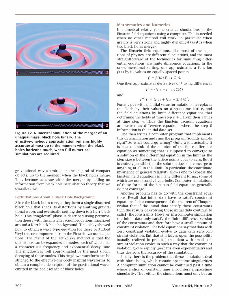
Figure 13. Numerical simulation of the ringdown afterthe merger of an unequal-mass, black hole binary. Inthe ringdown phase, perturbation theory provides anexcellent approximation to the waveform.

for a short amount of time, or the time slices inside theblack hole must somehow be “slowed down” so that theydo not encounter the singularity. But then if the time sliceadvances slowly inside the black hole and rapidly outsideit, this will lead to the slice being stretched in such away as to lead to inaccuracies in the finite differenceapproximation.

Before 2005 these three difficulties were insurmount-able, and none of the computer simulations of collidingblack holes gave anything that could be used to comparewith observations. Then suddenly in 2005 all of theseproblems were solved by Frans Pretorius, who producedthe first fully successful binary black hole simulation.Then later that year the problem was solved again (usingcompletely different methods!) by two other groups: oneconsisting of Campanelli, Lousto, Marronetti, and Zlo-chower and the other of Baker, Centrella, Choi, Koppitz,and van Meter. Though the methods are different, bothsets of solutions can be thought of as consisting of the in-gredients hyperbolicity, constraint damping, and excision,and we will treat each one in turn.

Hyperbolicity. Since one needs the equations to bestrongly hyperbolic, one could perform the simulationsinharmonic coordinates.However, onealsoneeds the timecoordinate to remain timelike, so instead Pretorius usedgeneralized harmonic coordinates (as first suggested byFriedrich) where the coordinates satisfy a wave equation

with a source. The other groups implemented hyperbolic-ity by using the BSSN equations (named for its inventors:Baumgarte, Shapiro, Shibata, and Nakamura). These equa-tions decompose the spatial metric into a conformalfactor and a metric of unit determinant and then evolveeach of these quantities separately, adding appropriateamounts of the constraint equations to convert the spatialRicci tensor into an elliptic operator.

Constraint damping. Because the constraints are zeroin exact solutions to the theory, one has the freedom toadd any multiples of the constraints to the right-handside of the field equations without changing the class ofsolutions to the field equations. In particular, with cleverchoices of which multiples of the constraints go on theright-hand side, one can arrange that in these newversionsof the field equations small violations of the constraintsget smaller under evolution rather than growing. CarstenGundlach showed how to do this for evolution usingharmonic coordinates, and his method was implementedby Pretorius. The BSSN equations already have somerearrangement of the constraint and evolution equations.Theparticular choice of lapse and shift (Φ and𝑋 fromeqns.(7–8)) used by the other groups (called 1+log slicing andGamma driver shift) were found to have good constraintdamping properties.

Excision. Because nothing can escape from a blackhole, nothing that happens inside can have any influenceon anything that happens outside. Thus in performingcomputer simulations of colliding black holes, one isallowed to simply excise the black hole interior from thecomputational grid and still obtain the answer to thequestion of what happens outside the black holes. Byexcising, one no longer has to worry about singularities orgrid stretching. Excision was first proposed by Unruh andThornburg, and first implemented by Seidel and Suen,and used in Pretorius’ simulations. The other groupsessentially achieve excision by other methods. They usea “moving puncture method” that involves a secondasymptotically flat end inside each black hole, which iscompactified to a single point that can move around thecomputational grid. The region between the puncture andthe black hole event horizon undergoes enormous gridstretching, so that effectively only the exterior of the blackhole is covered by the numerical grid.

Since 2005, many simulations of binary black holemergers have been performed, for various black holemasses and spins. Some of the most efficient simulationsare done by the SXS collaboration using spectral methodsinstead of finite difference methods. (SXS stands for“Simulating eXtreme Spacetimes” and the collaborationis based at Cornell, Caltech, and elsewhere.) Spectralmethodsuse the grid values 𝑓𝑖 to approximate the function𝑓(𝑥) as an expansion in a particular basis of orthogonalfunctions. The expansion coefficients and the derivativesof the basis functions are then used to compute thederivatives of 𝑓(𝑥). Compared tofinite differencemethods,spectral methods can achieve a given accuracy of thederivatives with significantly fewer grid points.


Gravitational Wave ExperimentThe experimental search for gravitational waves startedin the 1960s through the construction of resonant bardetectors. These essentially consist of a large (meter-size) cylinder in a vacuum chamber that is isolatedfrom vibrations. When a gravitational wave at the rightfrequency interacts with such a bar, it can excite thelatter’s resonant mode, producing a change in length thatone can search for. In 1968, Joseph Weber announcedthat he had detected gravitational waves with one suchresonant bar. The sensitivity of Weber’s resonant barto gravitational waves was not high enough for this tobe possible, and other groups could not reproduce hisexperiment.

Figure 14. Schematic diagram of a Michelsoninterferometer, which is at the heart of theinstrumental design used by aLIGO. In the diagram, alaser beam is split into two sub-beams that traveldown orthogonal arms, bounce off mirrors, and thenreturn to recombine.

In the late 1960s and early 1970s, the search for gravita-tional waves with laser interferometers began through thepioneering work of Rainer Weiss at MIT and Kip Thorneand Ronald Drever at Caltech, among many others. Thebasic idea behind interferometry is to split a laser beaminto two sub-beams that travel down orthogonal arms,bounce off mirrors, and then return to recombine. Ifthe light travel time is the same in each sub-beam, thenthe light recombines constructively, but if a gravitationalwave goes through the detector, then the light travel timeis not the same in each arm and interference occurs.Gravitational wave interferometers are devices that usethis interference process to measure small changes inlight travel time very accurately so as to learn about thegravitational waves that produced them, and thus, in turn,about the properties of the source of gravitational waves.

The initial Laser Interferometer Gravitational-Wave Ob-servatory (iLIGO) was funded by the National Science

Figure 15. (from top to bottom) Ronald Drever, KipThorne, and Rainer Weiss pioneered the effort todetect gravitational waves with laser interferometers.


Foundation in the early 1990s and operations started inthe early 2000s. There are actually two LIGO facilities (onein Hanford, Washington, and one in Livingston, Louisiana)in operation right now, with an Italian counterpart (Virgo)coming online soon, a Japanese counterpart (KAGRA)coming online by the end of the decade, and an Indiancounterpart (LIGO-India) coming online in the 2020s. Thereason for multiple detectors is to achieve redundancyand increase the confidence of a detection by observingthe signal by independent detectors with uncorrelatednoise. Although iLIGO was over four orders of magnitudemore sensitive than Weber’s original instrument in a widefrequency band, no gravitational waves were detected.

Figure 16. One of the two aLIGO facilities, this one inLivingston, Louisiana, where the interference patternassociated with a gravitational wave produced in themerger of two black holes was recorded within daysof the first science run.

In the late 2000s, upgrades to convert iLIGO intoadvanced LIGO (aLIGO) commenced. These upgrades in-cluded an increase in the laser power to reduce quantumnoise, larger and heavier mirrors to reduce thermal andradiation pressure noise, better suspension fibers for themirrors to reduce suspension thermal noise, amongmanyother improvements. aLIGO commenced science opera-tions in 2015 with a sensitivity roughly 3–4 times greaterthan that of iLIGO’s last science run.

Within days of the first science run, the aLIGO detec-tors recorded the interference pattern associated with agravitational wave produced in the merger of two blackholes 1.3 billion light years away. The signal was so loud(relative to the level of the noise) that the probability thatthe recorded event was a gravitational wave was muchlarger than 5𝜎, meaning that the probability of a falsealarm was much smaller than 10−7. There is no doubtthat this event, recorded on September 14, 2015, as wellas a second one, detected the day after Christmas of thatsame year, were the first direct detections of gravitationalwaves.

In order to understand how gravitational waves aredetected, we must understand how the waves affect themotion of the parts of the interferometer. The mirrorsare suspended from wires like a pendulum, but thismeans that for short time motion in the horizontaldirection, the motion of each mirror can be treated as

Figure 17. Top: Filtered GW strain as a function oftime detected at the Hanford location of aLIGO.Bottom: Best fit reconstruction of the signal using anumerical relativity simulation (red), an analyticalwaveform template (gray), and a set of Morleywavelets. The latter two are shown as 90 percentconfidence regions, while the simulation is aparticular run with a choice of parameters within thisthe 90 percent confidence region.

a spacetime geodesic. But the interferometer measuresdistance between the mirrors, so what we want to knowis how this distance changes under the influence of agravitational wave. The answer to this question comesfrom the Jacobi equation: the relative acceleration ofnearby geodesics is equal to the Riemann tensor timesthe separation of those geodesics.

Listen to theuniverse with

gravity.

Thus if at any timewe want to know theseparation, we needto integrate the Jacobiequation twice with re-spect to time.However,the Riemann tensor isthe second derivativeof the 𝑇𝑇 gauge met-ric perturbation. Thus, by using this particular gauge wecan say that LIGO directly measures the metric perturba-tion by using laser interferometry to keep track of theseparation of its mirrors.

Astrophysics and Fundamental PhysicsUp until now, we have created a picture of the universefrom the information we have obtained from amazingtelescopes, such as Chandra in the X-rays, Hubble in the


optical, Spitzer in the infrared, WMAP in the microwave,and Arecibo in the radio frequencies. This informationwas provided by light that traveled from astrophysicalsources to Earth. Every time humankind built a newtelescope that gave us access to a new frequency rangeof the light spectrum, amazing discoveries were made.The discovery of accretion disk signatures of black holesusing X-ray astronomy is a case in point. This expectationis especially true for gravitational wave detectors, whichdo not just open a new frequency range, but rather aim tolisten to the universe in an entirely new way: with gravityinstead of light.

This new type of astrophysics has an immense potentialto truly revolutionize science because gravitational wavescan provide very clean information about their sources.Unlike light, gravitational waves are very weakly coupledtomatter, allowing gravitational waves to go right throughthe intermediate matter (which would absorb light) andprovide a clean picture (or soundtrack) of astrophysicalsources that until now had remained obscure. Of course,this is a double-edged sword because the detection ofgravitational waves is extremely challenging, requiringthe ability to measure distances that are as small as 10−3

times the size of a proton over a 4 km baseline.The aLIGO detectors achieved just that, providing

humanity with not only the first direct detection ofgravitational waves, but also the first direct evidence ofthe existence of black hole binaries and their coalescence.As of the writing of this article, aLIGO had detected twoevents, both of which correspond to the coalescence ofbinary black hole systems in a quasi-circular orbit. Fittingthe hybrid analytic and numerical models described inthe sections “Approximation Methods” and “Mathematicsand Numerics” to the data, the aLIGO collaboration foundthat the first event consisted of two black holes withmasses

(𝑚1,𝑚2) ≈ (36.2, 29.1)𝑀⊙,where 𝑀⊙ is the mass of our sun, colliding at roughly halfthe speed of light to produce a remnant black hole withmass

𝑚𝑓 ≈ 62.3𝑀⊙

and dimensionless spin angular momentum

|𝑆|/𝑚2𝑓 ≈ 0.68,

located 420 mega-parsecs away from Earth (roughly 1.3billion times the distance light travels in one year). Thesecond event consisted of lighter black holes, withmasses

(𝑚1,𝑚2) ≈ (14.2, 7.5)𝑀⊙

that collided to produce a remnant black hole with mass𝑚𝑓 ≈ 20.8𝑀⊙

and dimensionless spin angular momentum

|𝑆|/𝑚2𝑓 ≈ 0.74,

located 440 mega-parsecs away from Earth. In both cases,the peak luminosity radiated was in the range of 1056

ergs/s with the systems effectively losing 3𝑀⊙ and 1𝑀⊙respectively in less than 0.1 seconds. Thus, for a very

brief moment, these events produced more energy thanall of the stars in the observable universe put together.

Perhaps one of the most interesting inferences onecan draw from such events is that black holes (or atthe very least, objects that look and “smell” a lot likeblack holes) truly do form binaries and truly do mergein nature within an amount of time smaller than the ageof the universe. Until now, we had inferred the existenceof black holes by either observing how other stars orbitaround supermassive ones at the center of galaxies or byobserving enormousdisks of gas orbit around stellarmassblack holes and the X-rays emitted as some of that gasfalls into the black hole. The aLIGO observations are thefirst direct observation of radiation produced by binaryblack holes themselves through the wave-like excitationsof the curvature they generate when they collide. Not onlydid the aLIGO observation prove the existence of binaryblack holes, but even the first observation brought abouta surprise: the existence and merger of black holes in amass range that had never been observed before.

Figure 18. Nicolás Yunes and his team exploremathematically the extreme gravity of black holesand neutron stars, as well as the gravitational wavesthey emit when they inspiral into each other andcollide. The goal of his research program is toconstruct analytic models that enable the extractionof the most astrophysics and theoretical physicsinformation from future astrophysics andgravitational wave observations, thus allowing us totest Einstein’s theory in the essentially unexploredextreme gravity regime.

The aLIGOobservations havedemonstrated that generalrelativity is not only highly accurate at describing gravi-tational phenomena in the solar system, in binary pulsarobservations, and in cosmological observations, but alsoin the late inspiral, merger, and ringdown of black hole bi-naries. Gravity is truly described by Einstein’s theory evenin the most extreme gravity scenarios: when the gravita-tional interaction is strong, highly nonlinear, and highlydynamical. Such consistency with Einstein’s theory hasimportant consequences on theories that modify gravity


in hopes of arriving at a quantum gravitational comple-tion. Future gravitational wave observations will allow usto verify many other pillars of Einstein’s theory, such asthat the gravitational interaction is parity invariant, thatgravitational waves propagate at the speed of light, andthat it only possesses two transverse polarizations.

The detection of gravitational waves is not only aspectacular confirmation of Einstein’s theory, but alsothe beginning of a new era in astrophysics. Gravitationalwaves will provide the soundtrack to the movie of ouruniverse, a soundtrack we had so far been missing withtelescopes. No doubt that they will be a rich sourcefor new questions and inspiration in physics as wellas mathematics. We wait anxiously for the unexpectedbeauty this music will provide.

AcknowledgmentsThe authors acknowledge their NSF support. The first au-thor was supported by NSF CAREER grant DMS-1253149to the University of Michigan. The second author wassupported by NSF grant PHY-1505565 to Oakland Univer-sity. The third author acknowledges support from NSFCAREER Grant PHY-1250636.

References[1] LIGO Scientific Collaboration and Virgo Collaboration; Ab-

bott, B.P., et al., Observation of Gravitational Waves fromBinary Black Hole Merger, Physical Review Letters 116.061102. (2016).

[2] Y. Choquet-Bruhat, Théorème d’existence pour certain sys-tèmes d’equations aux dérivées partielles nonlinéaires, ActaMath. 88 (1952), 141–225.

[3] Y. Choquet-Bruhat and R. Geroch, Global Aspects of theCauchy Problem in General Relativity, Comm. Math. Phys. 14(1969), 329–335.

[4] A. Einstein, Näherungsweise Integration der Feldgleichun-gen der Gravitation, SAW (Sitzungsber. K. Preuss. Akad. Wiss.Berlin) (1916), 688–696.

Photo CreditsFigures 1 and 4 are in the public domain.Figures 2, 3, and 9 are courtesy of Christina Sormani.Figure 5 is courtesy of the Archives of the MathematischesForschungsinstitut Oberwolfach.Figures 6, 7, and 8 are courtesy of Lydia Bieri.Figure 10 is courtesy of David Garfinkle.Figures 11, 12, and 13 are courtesy of S. Ossokine, A. Buonanno,T. Dietrich, and R. Haas (Max Planck Institute for GravitationalPhysics), Simulating eXtreme Spacetimes project.Figure 14 is courtesy of Ed Stanner.Figure 15 is courtesy of the Gruber Foundation.Figure 16 is courtesy of the Caltech/MIT/LIGO Lab.Figure 17 is courtesy of [1] B.P. Abbott et al. “Observationof Gravitational Waves from a Binary Black Hole Merger”Physical Review Letters 116, 061102 (2016) DOI: 10.1103/Phys-RevLett.116.061102.Figure 18 and author headshot are courtesy of Nicolás Yunes.Author headshot is courtesy of Lydia Bieri.Author headshot is courtesy of David Garfinkle.


Date post:	01-May-2018
Category:	Documents
Upload:	lamdien
View:	217 times
Download:	2 times

THE MATHEMATICS OF GRAVITATIONAL WAVES ... MATHEMATICS OF GRAVITATIONAL WAVES This illustration...

Documents