Linear Vector Spaces : We’re familiar with ordinary vectors and the various ways we can manipulate them. Now let’s generalize this notion. We define a general vector to be an “object”, denoted , with the following properties. - PowerPoint PPT Presentation
THE MATHEMATICS OF QUANTUM MECHANICS Linear Vector Spaces : We’re familiar with ordinary vectors and the various ways we can manipulate them Now let’s generalize this notion. We define a general vector to be an “object”, denoted , with the following properties plus all the usual laws of associativity, distributivity, and commutivity. Together, a collection of vectors with the associated properties is called a linear vector space . (Reading: Shankar Chpt. 1; Griffiths appendix, 3.1- 3.3, 3.6)
Transcript
THE MATHEMATICS OF QUANTUM MECHANICS
Linear Vector Spaces:
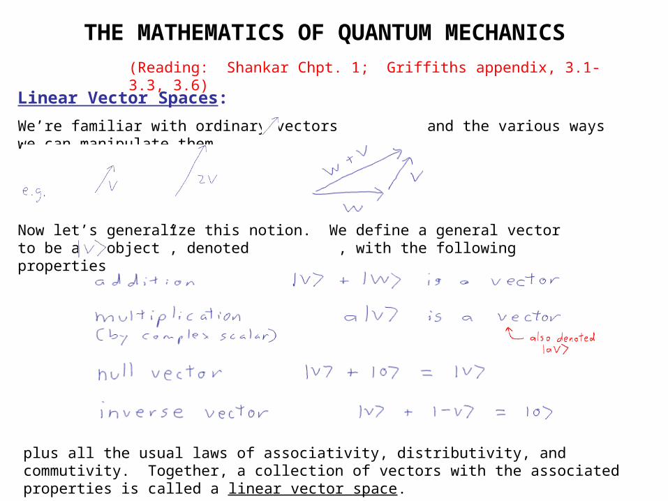
We’re familiar with ordinary vectors and the various ways we can manipulate them
Now let’s generalize this notion. We define a general vector to be an “object”, denoted , with the following properties
plus all the usual laws of associativity, distributivity, and commutivity. Together, a collection of vectors with the associated properties is called a linear vector space.
Why do we care about vector spaces? Because in quantum mechanics, the state of a physical system can be described by vectors!
Linear Independence and Basis Vectors
A set of vectors is linearly independent if the only solution
to
is when all coefficients vanish: ai=0 for all i =1..N
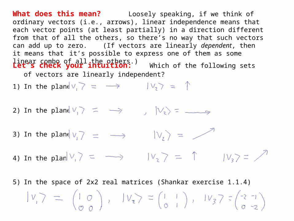
What does this mean? Loosely speaking, if we think of ordinary vectors (i.e., arrows), linear independence means that each vector points (at least partially) in a direction different from that of all the others, so there’s no way that such vectors can add up to zero. (If vectors are linearly dependent, then it means that it’s possible to express one of them as some linear combo of all the others.)
Let’s check your intuition: Which of the following sets of vectors are linearly independent?
1) In the plane,
2) In the plane,
3) In the plane,
4) In the plane,
5) In the space of 2x2 real matrices (Shankar exercise 1.1.4)
Some terminology: The dimension of the vector space is the maximum number of linearly independent vectors the vector space can have.
A set of N linearly independent vectors in an N-dimensional vector space is called a “basis” for the vector space. The vectors of the basis are called “basis vectors” (very original!).
What’s the significance of a basis?
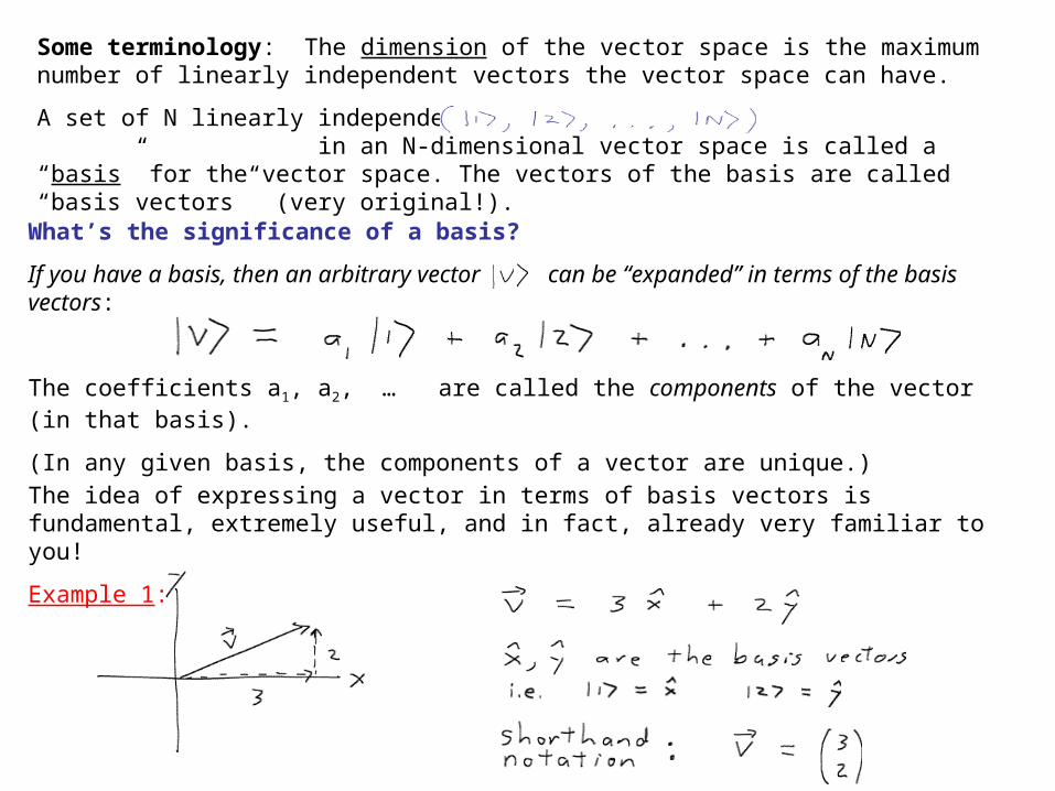
If you have a basis, then an arbitrary vector can be “expanded” in terms of the basis vectors:
The coefficients a1, a2, … are called the components of the vector (in that basis).
(In any given basis, the components of a vector are unique.)
The idea of expressing a vector in terms of basis vectors is fundamental, extremely useful, and in fact, already very familiar to you!
Example 1:
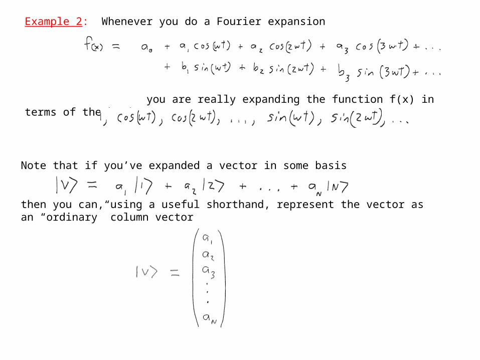
Example 2: Whenever you do a Fourier expansion
you are really expanding the function f(x) in terms of the basis vectors
Note that if you’ve expanded a vector in some basis
then you can, using a useful shorthand, represent the vector as an “ordinary” column vector
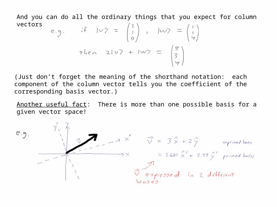
And you can do all the ordinary things that you expect for column vectors
(Just don’t forget the meaning of the shorthand notation: each component of the column vector tells you the coefficient of the corresponding basis vector.)
Another useful fact: There is more than one possible basis for a given vector space!
(Notice how the same vector can look very different depending on the basis! -- but it contains all the same information regardless of how it’s expressed.)
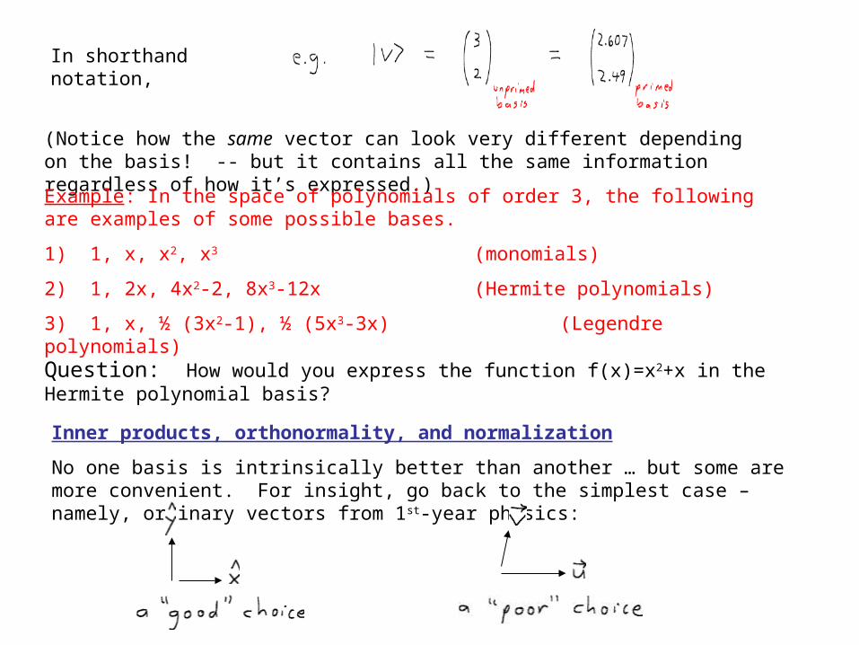
In shorthand notation,
Example: In the space of polynomials of order 3, the following are examples of some possible bases.
1) 1, x, x2, x3 (monomials)
2) 1, 2x, 4x2-2, 8x3-12x (Hermite polynomials)
3) 1, x, ½ (3x2-1), ½ (5x3-3x) (Legendre polynomials)
Question: How would you express the function f(x)=x2+x in the Hermite polynomial basis?
Inner products, orthonormality, and normalization
No one basis is intrinsically better than another … but some are more convenient. For insight, go back to the simplest case – namely, ordinary vectors from 1st-year physics:
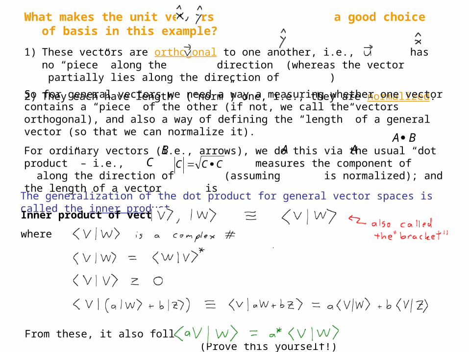
What makes the unit vectors a good choice of basis in this example?
1) These vectors are orthogonal to one another, i.e., has no “piece” along the direction (whereas the vector partially lies along the direction of )
2) They each have length (“norm”) one, i.e., they are normalized.
So for general vectors we need a way a measuring whether one vector contains a “piece” of the other (if not, we call the vectors orthogonal), and also a way of defining the “length” of a general vector (so that we can normalize it).
For ordinary vectors (i.e., arrows), we do this via the usual “dot product” – i.e., measures the component of along the direction of (assuming is normalized); and the length of a vector is
BA
A
B
A
C
CCC
The generalization of the dot product for general vector spaces is called the inner product.
Inner product of vectors
where
From these, it also follows that (Prove this yourself!)
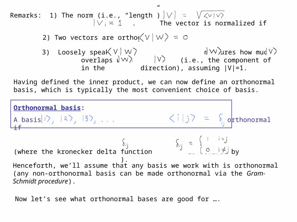
Remarks: 1) The norm (i.e., “length”) of a vector is . The vector is normalized if
2) Two vectors are orthogonal if
3) Loosely speaking, measures how much overlaps with (i.e., the component of in the direction), assuming |V|=1.
Having defined the inner product, we can now define an orthonormal basis, which is typically the most convenient choice of basis.
Orthonormal basis:
A basis is orthonormal if
(where the kronecker delta function is defined by ).
Henceforth, we’ll assume that any basis we work with is orthonormal (any non-orthonormal basis can be made orthonormal via the Gram-Schmidt procedure).
Now let’s see what orthonormal bases are good for ….
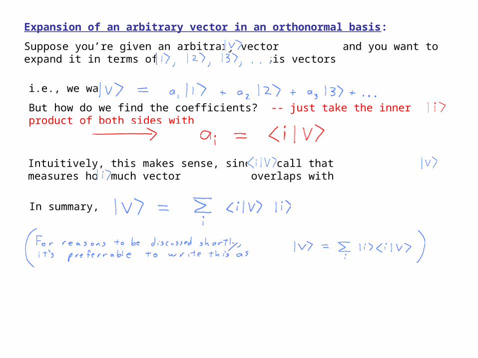
Expansion of an arbitrary vector in an orthonormal basis:
Suppose you’re given an arbitrary vector and you want to expand it in terms of (orthonormal) basis vectors
i.e., we want
But how do we find the coefficients? -- just take the inner product of both sides with
Intuitively, this makes sense, since recall that measures how much vector overlaps with
In summary,
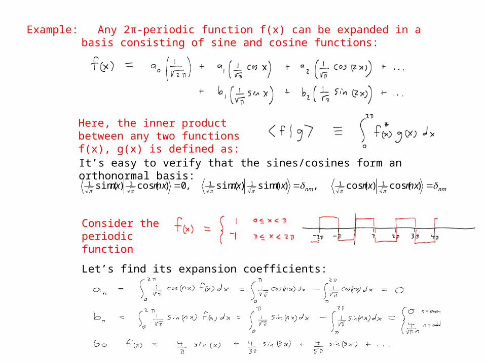
Example: Any 2π-periodic function f(x) can be expanded in a basis consisting of sine and cosine functions:
Here, the inner product between any two functions f(x), g(x) is defined as:
It’s easy to verify that the sines/cosines form an orthonormal basis:
nmnm mxnxmxnxmxnx
)cos()cos( ,)sin()sin( ,0)cos()sin( 111111
Consider the periodic function
Let’s find its expansion coefficients:
Inner products of vectors in an orthonormal basis:
Given two expanded vectors, , their inner
product takes on a particularly simple form:
(Note the similarity to the ordinary dot product: )
332211 bababaBA
In fact, if we write each vector as a column vector
then the inner product (“bracket”) can be written
Stop and prove this yourself!
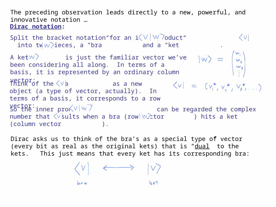
The preceding observation leads directly to a new, powerful, and innovative notation …
Dirac notation:
Split the bracket notation for an inner product into two pieces, a “bra” and a “ket” .
Think of the bra as a new object (a type of vector, actually). In terms of a basis, it corresponds to a row vector:
A ket is just the familiar vector we’ve been considering all along. In terms of a basis, it is represented by an ordinary column vector:
So the inner product can be regarded the complex number that results when a bra (row vector ) hits a ket (column vector ).
Dirac asks us to think of the bra’s as a special type of vector (every bit as real as the original kets) that is “dual” to the kets. This just means that every ket has its corresponding bra:
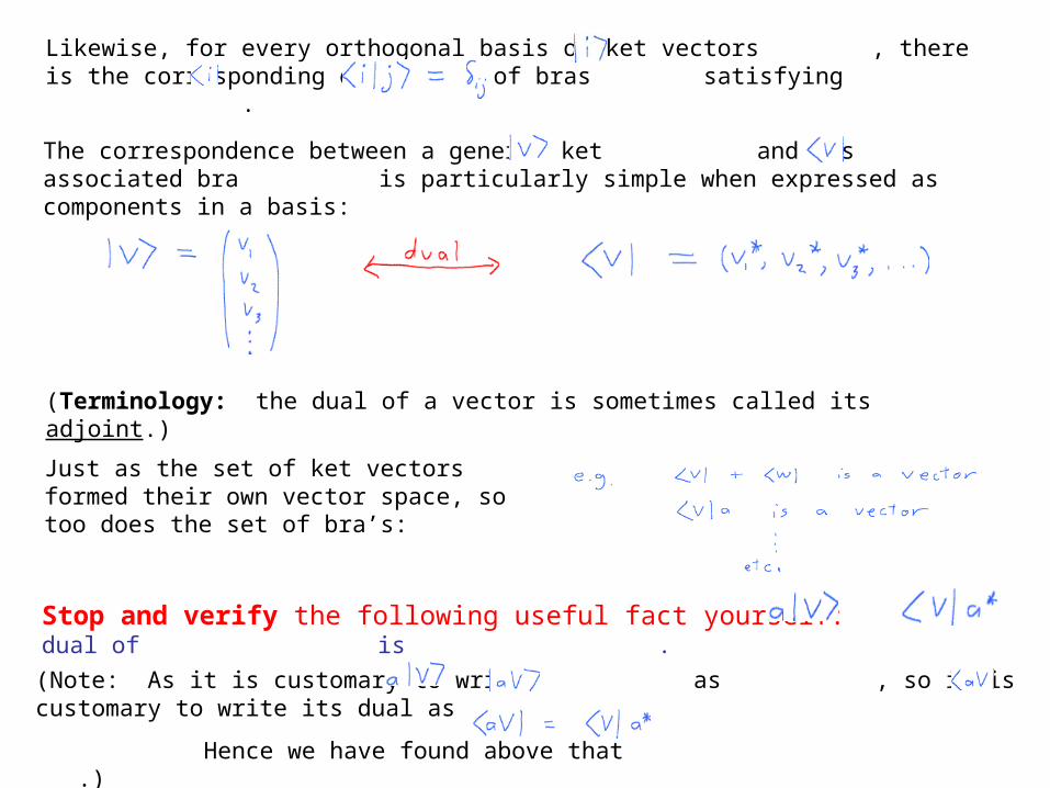
Likewise, for every orthogonal basis of ket vectors , there is the corresponding dual basis of bras satisfying .
Just as the set of ket vectors formed their own vector space, so too does the set of bra’s:
Stop and verify the following useful fact yourself: The dual of is .
(Note: As it is customary to write as , so it is customary to write its dual as .
Hence we have found above that .)
The correspondence between a general ket and its associated bra is particularly simple when expressed as components in a basis:
(Terminology: the dual of a vector is sometimes called its adjoint.)
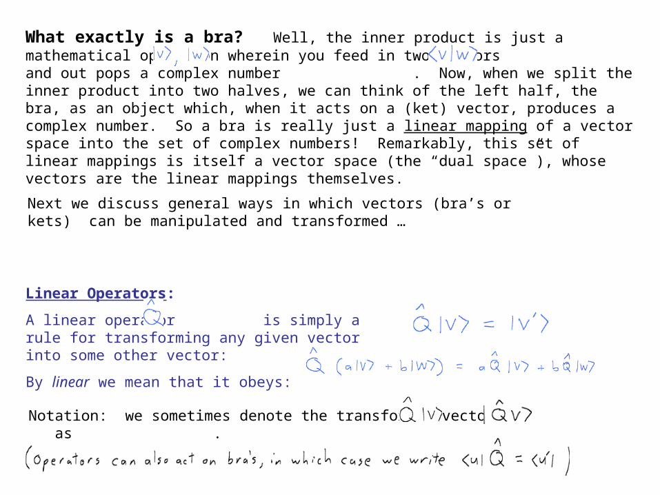
What exactly is a bra? Well, the inner product is just a mathematical operation wherein you feed in two vectors and out pops a complex number . Now, when we split the inner product into two halves, we can think of the left half, the bra, as an object which, when it acts on a (ket) vector, produces a complex number. So a bra is really just a linear mapping of a vector space into the set of complex numbers! Remarkably, this set of linear mappings is itself a vector space (the “dual space”), whose vectors are the linear mappings themselves.
Next we discuss general ways in which vectors (bra’s or kets) can be manipulated and transformed …
Linear Operators:
A linear operator is simply a rule for transforming any given vector into some other vector:
By linear we mean that it obeys:
Notation: we sometimes denote the transformed vector as .
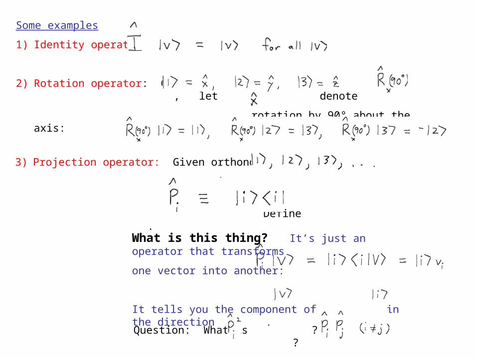
Some examples
1) Identity operator:
2) Rotation operator: Given , let denote
rotation by 90° about the axis:
3) Projection operator: Given orthonormal basis ,
Define .
What is this thing? It’s just an operator that transforms
one vector into another:
It tells you the component of in the direction .
Question: What is ? How about ?
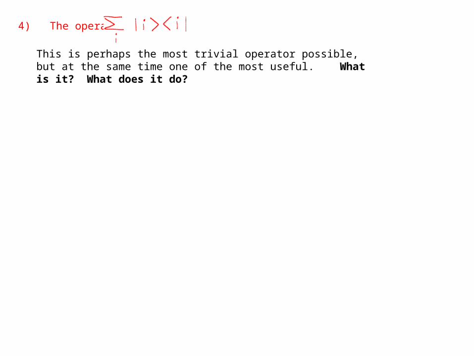
4) The operator
This is perhaps the most trivial operator possible, but at the same time one of the most useful. What is it? What does it do?
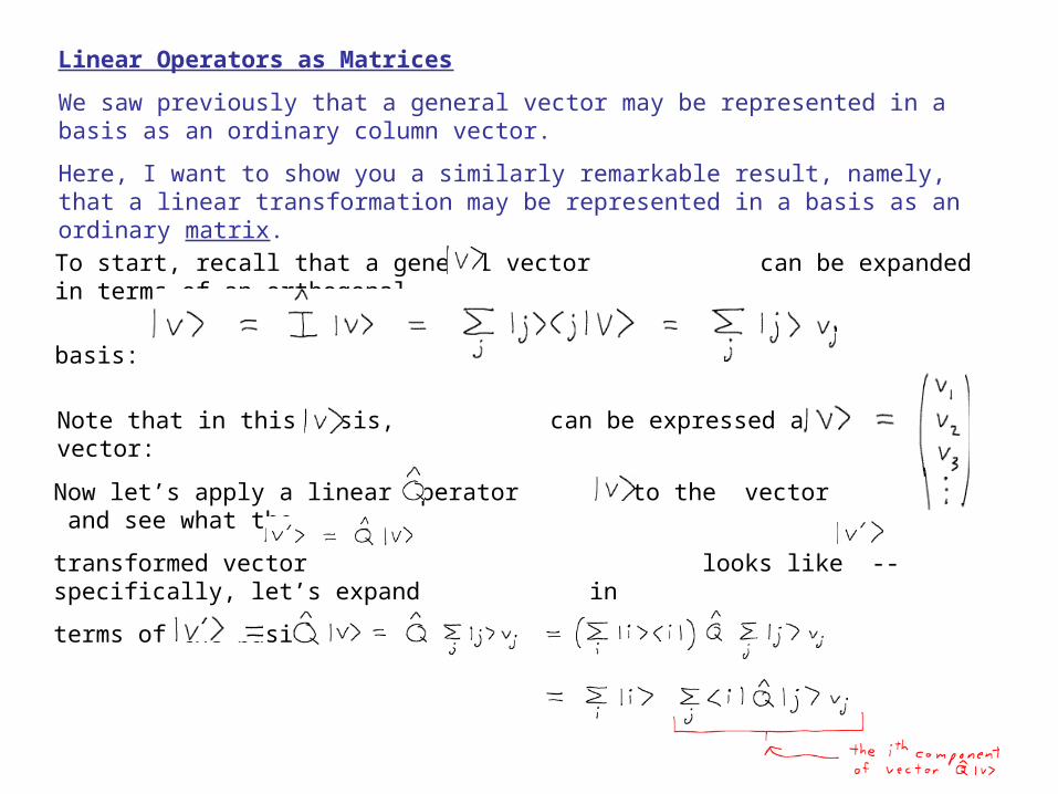
Linear Operators as Matrices
We saw previously that a general vector may be represented in a basis as an ordinary column vector.
Here, I want to show you a similarly remarkable result, namely, that a linear transformation may be represented in a basis as an ordinary matrix.
To start, recall that a general vector can be expanded in terms of an orthogonal
basis:
Note that in this basis, can be expressed as a column vector:
Now let’s apply a linear operator to the vector and see what the
transformed vector looks like -- specifically, let’s expand in
terms of the basis:
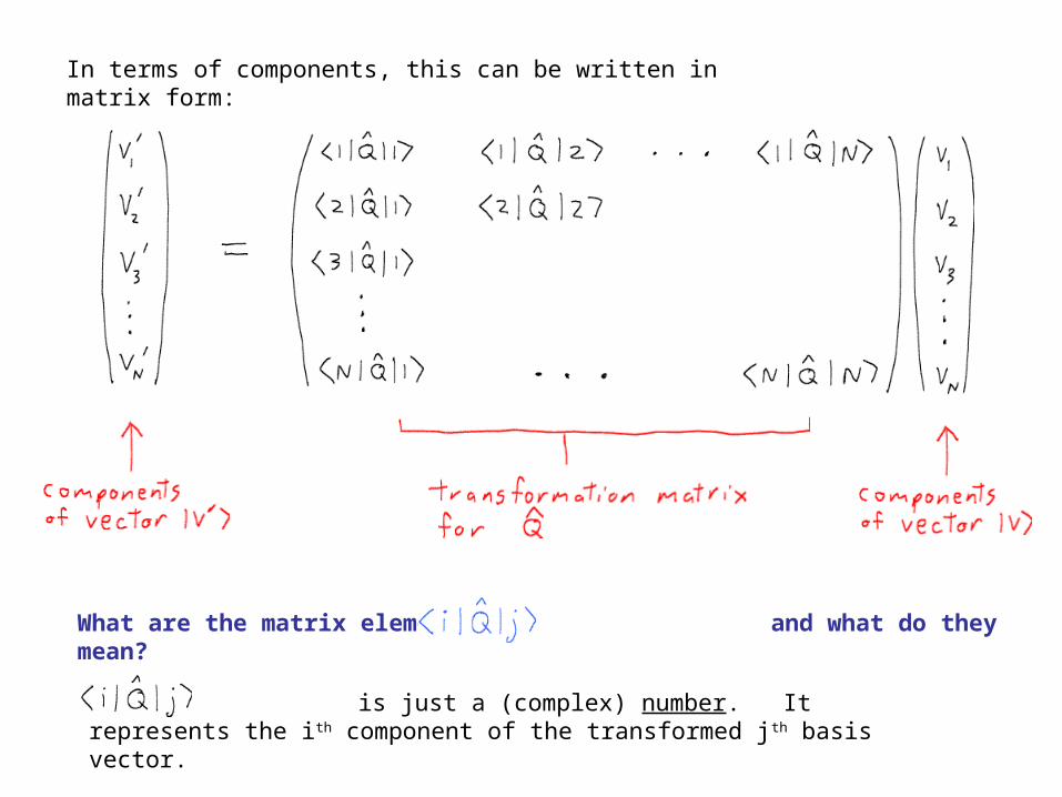
In terms of components, this can be written in matrix form:
What are the matrix elements and what do they mean?
is just a (complex) number. It represents the ith component of the transformed jth basis vector.
Stop and try this out: Write the rotation operator introduced earlier in matrix notation, and then determine how a unit vector pointing at a 45° angle in the x-y plane will be rotated.
Properties of Operators and Special Classes of Operators:
1) The inverse of an operator , if it exists, is denoted .
Question: Is the rotation operator invertible? What about the projection operator?Question: What is the inverse of the product ?
Question: Give a familiar illustration of this. (Hint: think rotations)
2) If operators are applied in succession, the order in which they are applied matters:
The ability to express a linear operator (in a particular basis) as a matrix is very useful, and all the familiar rules about matrix multiplication apply!
e.g., if P,Q are matrices corresponding to operators , then the matrix
corresponding to the product of operators is simply the matrix product .
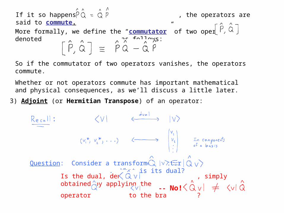
If it so happens that , the operators are said to commute.
More formally, we define the “commutator” of two operators, denoted , as follows:
So if the commutator of two operators vanishes, the operators commute.
Whether or not operators commute has important mathematical and physical consequences, as we’ll discuss a little later.
3) Adjoint (or Hermitian Transpose) of an operator:
Question: Consider a transformed vector . What is its dual? Is the dual, denoted , simply obtained by applying the
operator to the bra ? -- No!
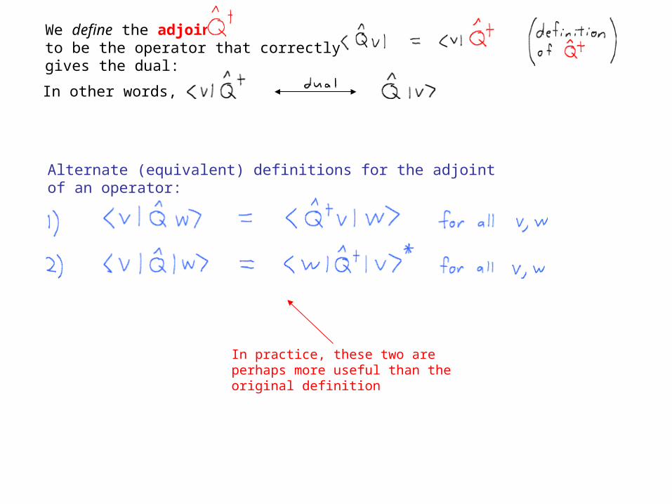
We define the adjoint to be the operator that correctly gives the dual:
In other words,
Alternate (equivalent) definitions for the adjoint of an operator:
In practice, these two are perhaps more useful than the original definition
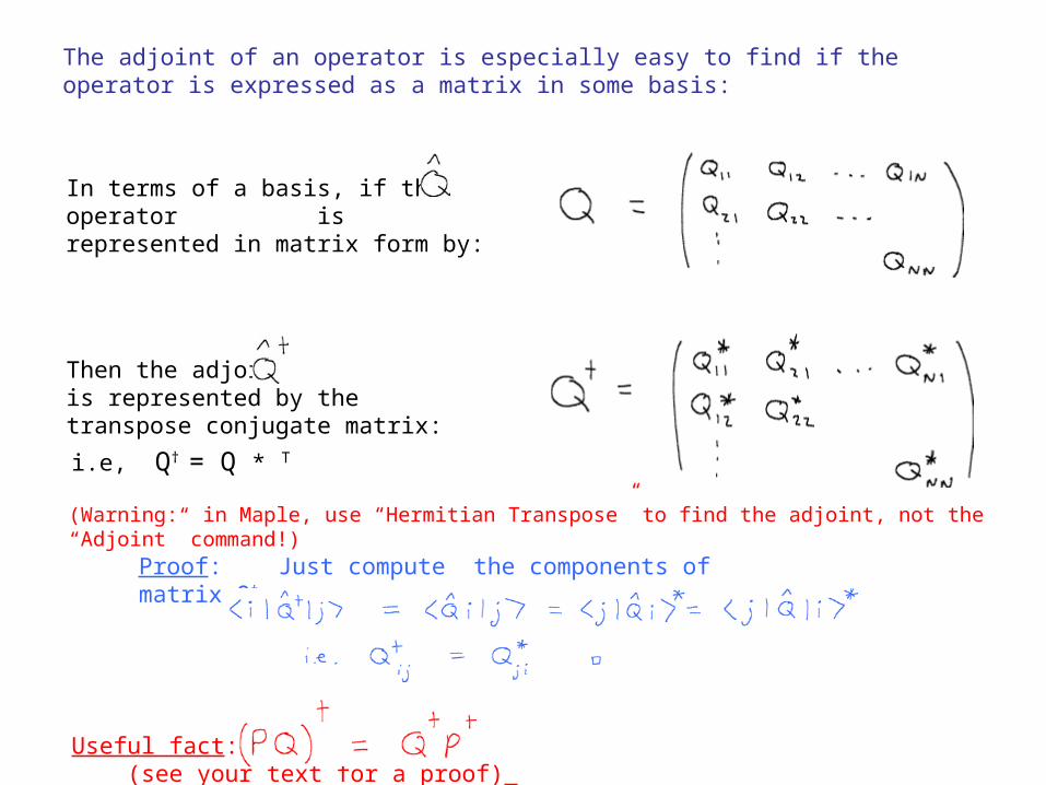
Proof: Just compute the components of matrix Q† :
Useful fact: (see your text for a proof)
The adjoint of an operator is especially easy to find if the operator is expressed as a matrix in some basis:
In terms of a basis, if the operator is represented in matrix form by:
Then the adjoint is represented by the transpose conjugate matrix:
i.e, Q† = Q * T
(Warning: in Maple, use “Hermitian Transpose” to find the adjoint, not the “Adjoint” command!)
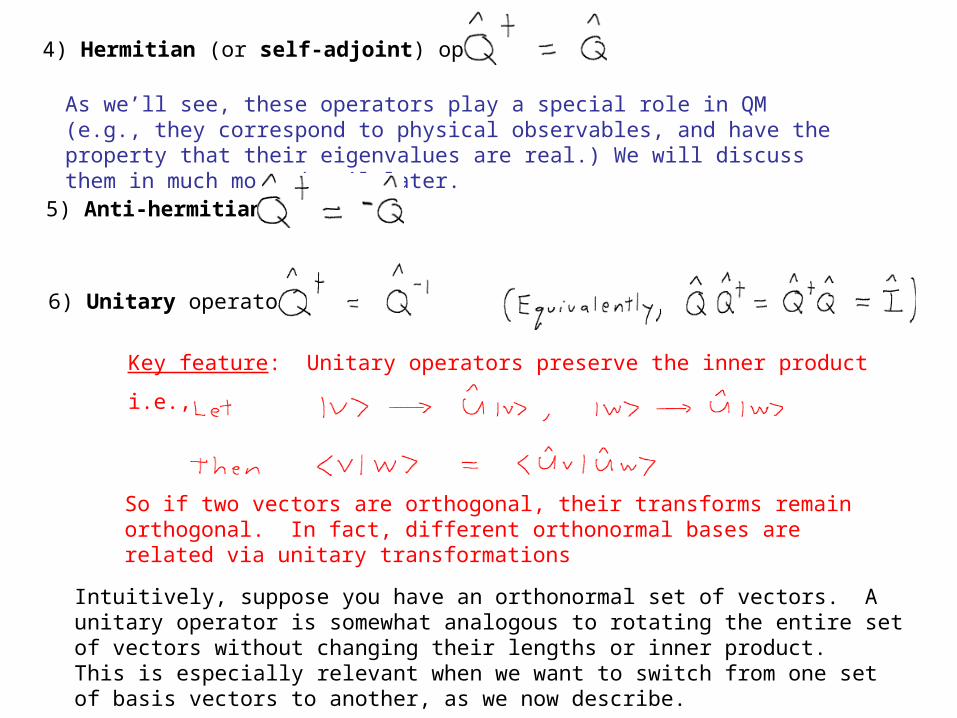
4) Hermitian (or self-adjoint) operators:
As we’ll see, these operators play a special role in QM (e.g., they correspond to physical observables, and have the property that their eigenvalues are real.) We will discuss them in much more detail later.
5) Anti-hermitian:
6) Unitary operators:
Key feature: Unitary operators preserve the inner product
i.e.,
So if two vectors are orthogonal, their transforms remain orthogonal. In fact, different orthonormal bases are related via unitary transformations
Intuitively, suppose you have an orthonormal set of vectors. A unitary operator is somewhat analogous to rotating the entire set of vectors without changing their lengths or inner product. This is especially relevant when we want to switch from one set of basis vectors to another, as we now describe.
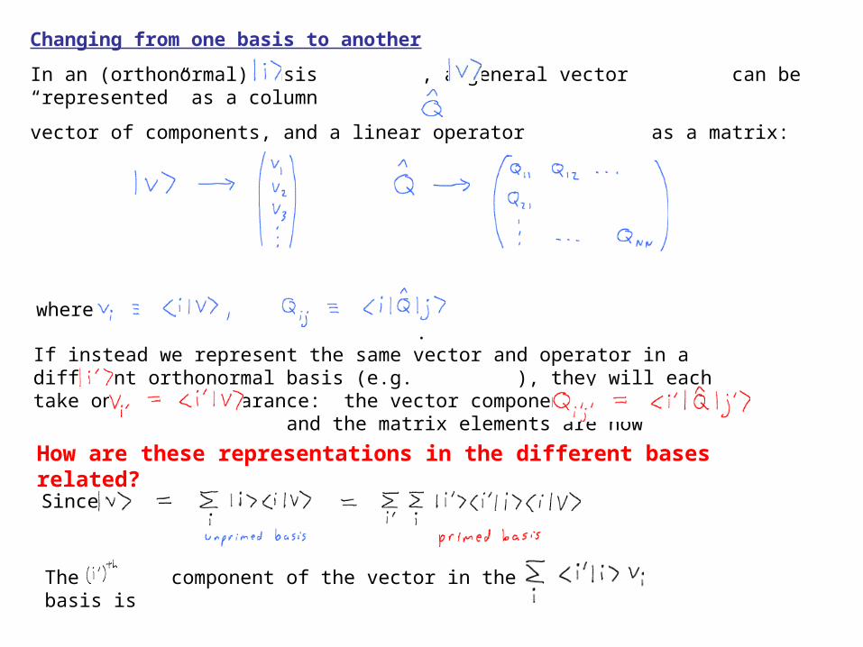
Changing from one basis to another
In an (orthonormal) basis , a general vector can be “represented” as a column
vector of components, and a linear operator as a matrix:
where .
If instead we represent the same vector and operator in a different orthonormal basis (e.g. ), they will each take on a new appearance: the vector components become and the matrix elements are now
How are these representations in the different bases related?Since
The component of the vector in the primed basis is
i.e., representations of a vector in different bases are related by a unitary transformation
whose matrix components are given above. More generally,
Hence, the vector components in the primed basis are related to those in the unprimed basis by
Next let’s look how a matrix associated with a linear operator changes appearance under a change of basis …
Stop and verify for yourself that the above transformation is indeed unitary!
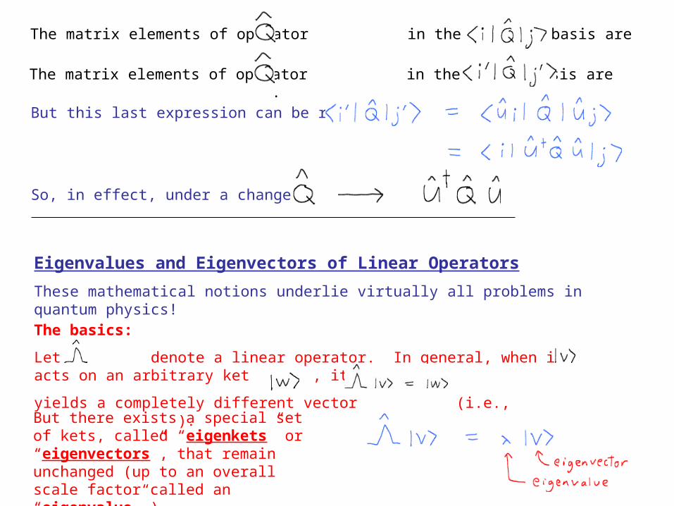
The matrix elements of operator in the unprimed basis are .
The matrix elements of operator in the primed basis are .
But this last expression can be rewritten as
So, in effect, under a change of basis,
Eigenvalues and Eigenvectors of Linear Operators
These mathematical notions underlie virtually all problems in quantum physics!
The basics:
Let denote a linear operator. In general, when it acts on an arbitrary ket , it
yields a completely different vector (i.e., ).
But there exists a special set of kets, called “eigenkets” or “eigenvectors”, that remain unchanged (up to an overall scale factor called an “eigenvalue” ).
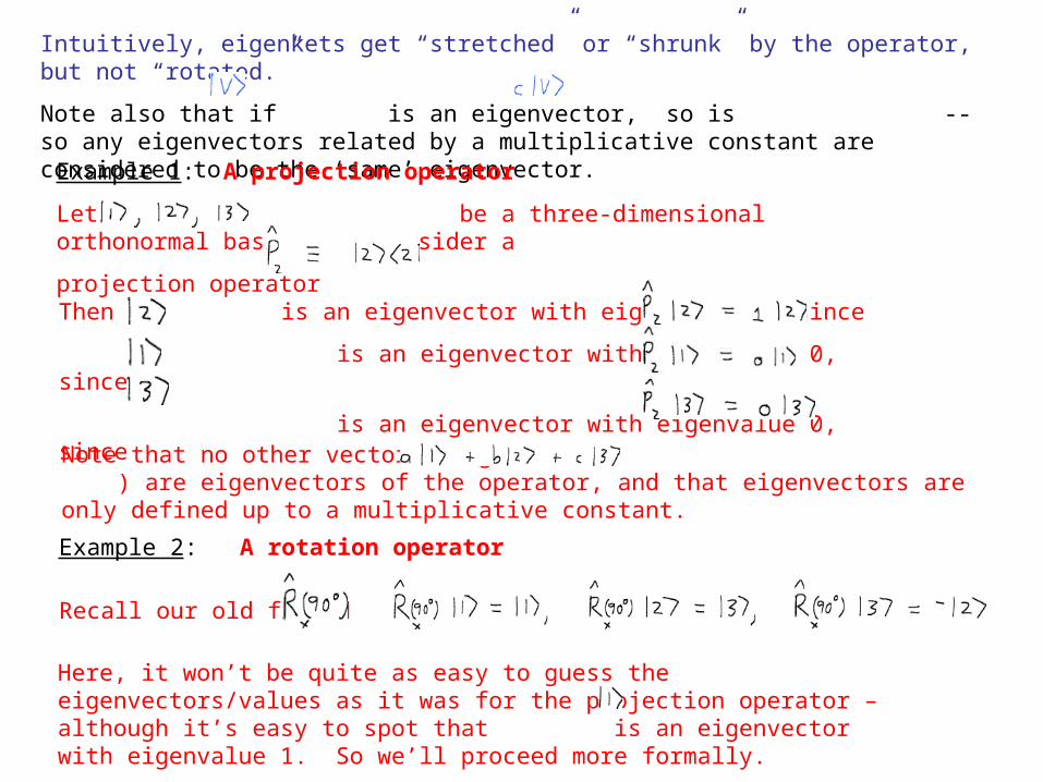
Intuitively, eigenkets get “stretched” or “shrunk” by the operator, but not “rotated.”
Note also that if is an eigenvector, so is -- so any eigenvectors related by a multiplicative constant are considered to be the ‘same’ eigenvector.
Example 1: A projection operator
Let be a three-dimensional orthonormal basis, and consider a
projection operator
Then is an eigenvector with eigenvalue 1, since
is an eigenvector with eigenvalue 0, since
is an eigenvector with eigenvalue 0, since
Note that no other vectors (e.g., ) are eigenvectors of the operator, and that eigenvectors are only defined up to a multiplicative constant.
Example 2: A rotation operator
Recall our old friend :
Here, it won’t be quite as easy to guess the eigenvectors/values as it was for the projection operator – although it’s easy to spot that is an eigenvector with eigenvalue 1. So we’ll proceed more formally.
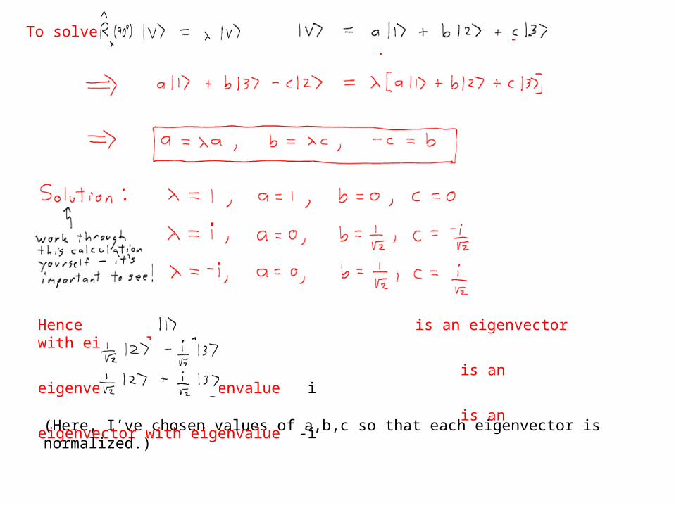
To solve , try .
Hence is an eigenvector with eigenvalue 1
is an eigenvector with eigenvalue i
is an eigenvector with eigenvalue -i
(Here, I’ve chosen values of a,b,c so that each eigenvector is normalized.)
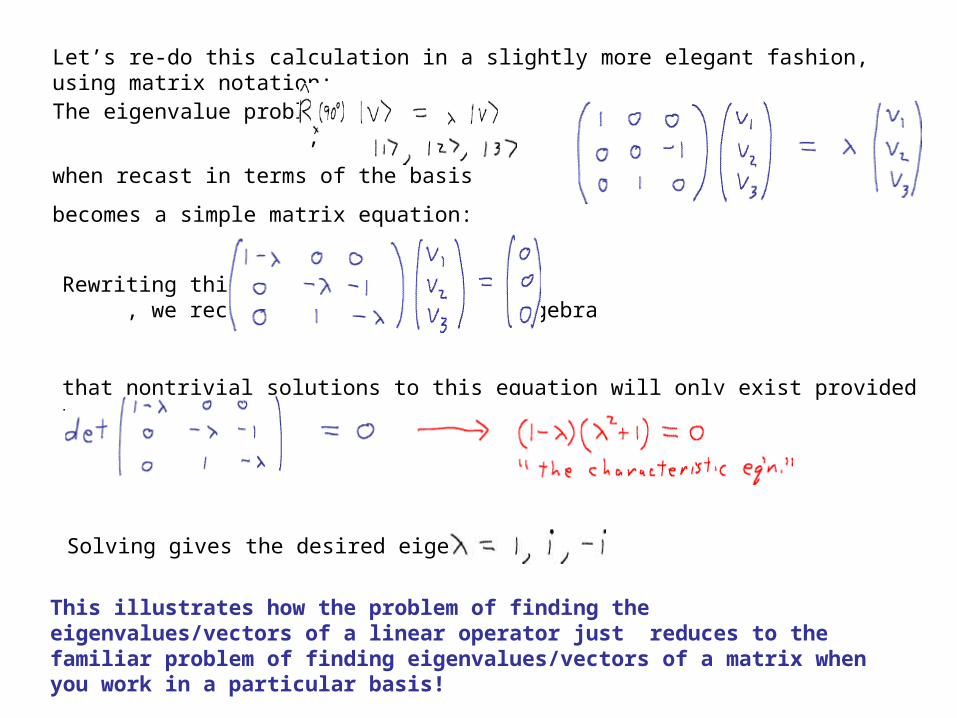
Let’s re-do this calculation in a slightly more elegant fashion, using matrix notation:
The eigenvalue problem, ,
when recast in terms of the basis
becomes a simple matrix equation:
Rewriting this as , we recall from basic linear algebra
that nontrivial solutions to this equation will only exist provided the determinant vanishes:
Solving gives the desired eigenvalues:
This illustrates how the problem of finding the eigenvalues/vectors of a linear operator just reduces to the familiar problem of finding eigenvalues/vectors of a matrix when you work in a particular basis!
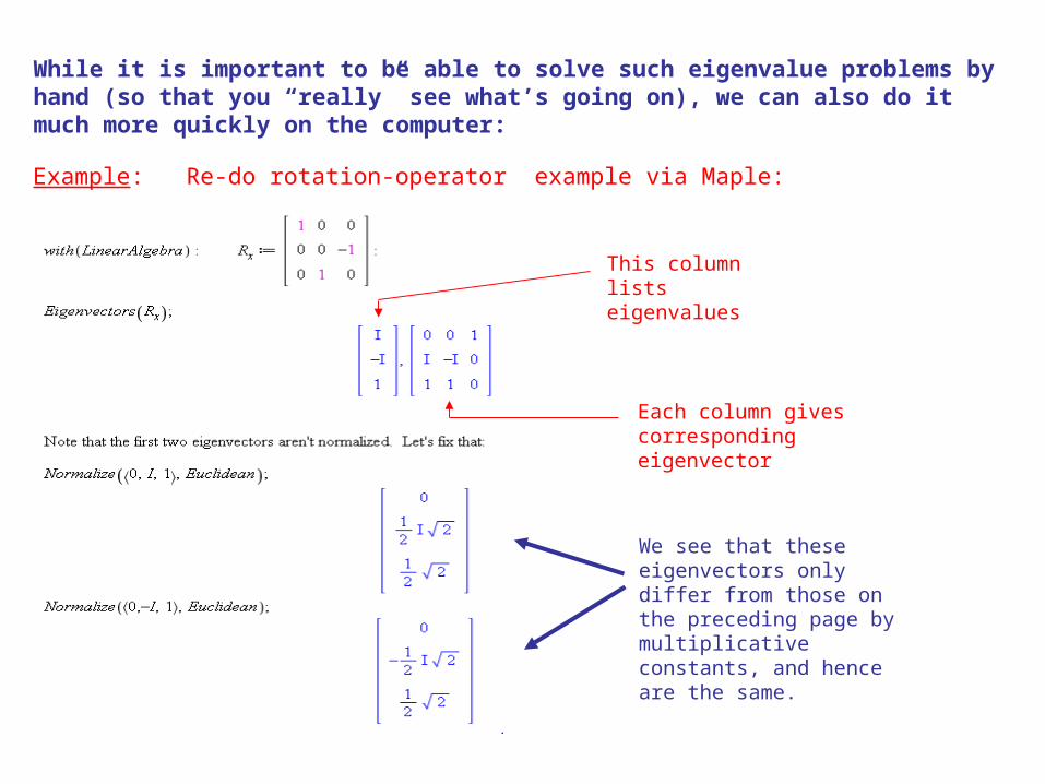
While it is important to be able to solve such eigenvalue problems by hand (so that you “really” see what’s going on), we can also do it much more quickly on the computer:
Example: Re-do rotation-operator example via Maple:
This column lists eigenvalues
Each column gives corresponding eigenvector
We see that these eigenvectors only differ from those on the preceding page by multiplicative constants, and hence are the same.
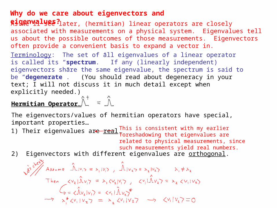
Why do we care about eigenvectors and eigenvalues?As we’ll see later, (hermitian) linear operators are closely associated with measurements on a physical system. Eigenvalues tell us about the possible outcomes of those measurements. Eigenvectors often provide a convenient basis to expand a vector in.
Terminology: The set of all eigenvalues of a linear operator is called its “spectrum.” If any (linearly independent) eigenvectors share the same eigenvalue, the spectrum is said to be “degenerate”. (You should read about degeneracy in your text; I will not discuss it in much detail except when explicitly needed.)
1) Their eigenvalues are real. This is consistent with my earlier foreshadowing that eigenvalues are related to physical measurements, since such measurements yield real numbers.
2) Eigenvectors with different eigenvalues are orthogonal.
Hermitian Operators
The eigenvectors/values of hermitian operators have special, important properties…
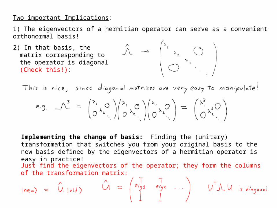
Two important Implications:
1) The eigenvectors of a hermitian operator can serve as a convenient orthonormal basis!
2) In that basis, the matrix corresponding to the operator is diagonal (Check this!):
Implementing the change of basis: Finding the (unitary) transformation that switches you from your original basis to the new basis defined by the eigenvectors of a hermitian operator is easy in practice!
Just find the eigenvectors of the operator; they form the columns of the transformation matrix:
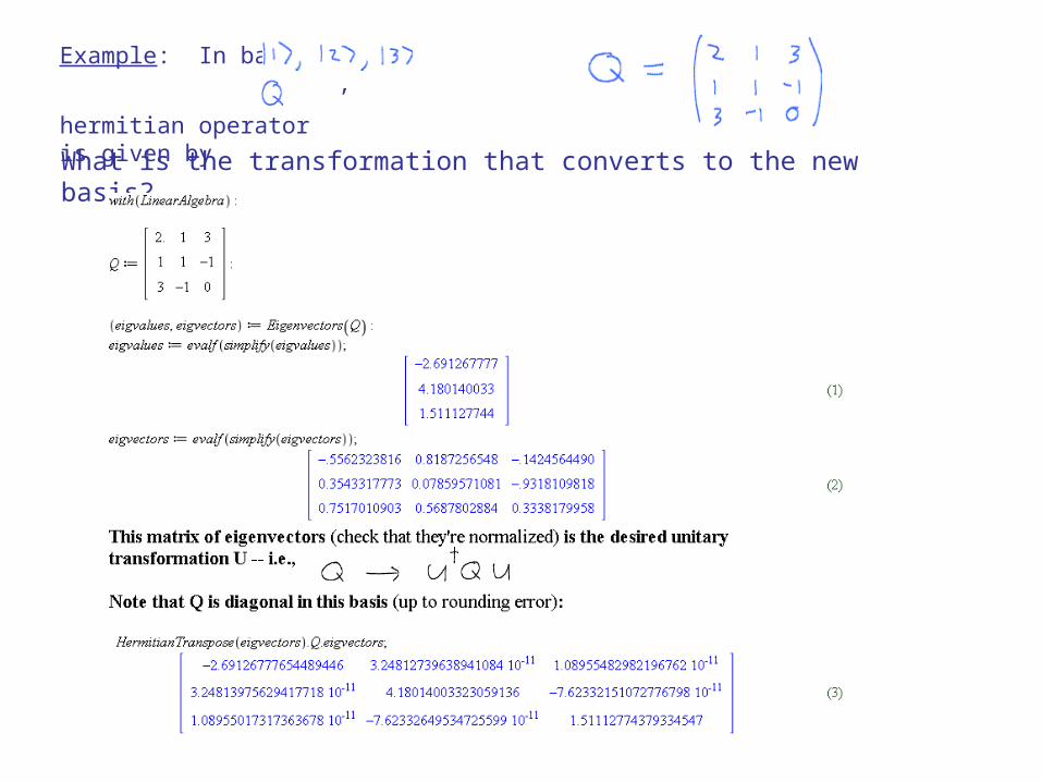
Example: In basis ,
hermitian operator is given by
What is the transformation that converts to the new basis?
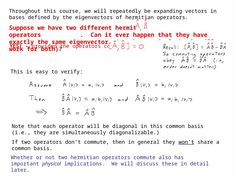
Throughout this course, we will repeatedly be expanding vectors in bases defined by the eigenvectors of hermitian operators.
Suppose we have two different hermitian operators . Can it ever happen that they have exactly the same eigenvectors (so that a single basis will work for both)?YES! – provided the operators commute
This is easy to verify:
Note that each operator will be diagonal in this common basis (i.e., they are simultaneously diagonalizable.)
If two operators don’t commute, then in general they won’t share a common basis.
Whether or not two hermitian operators commute also has important physical implications. We will discuss these in detail later.
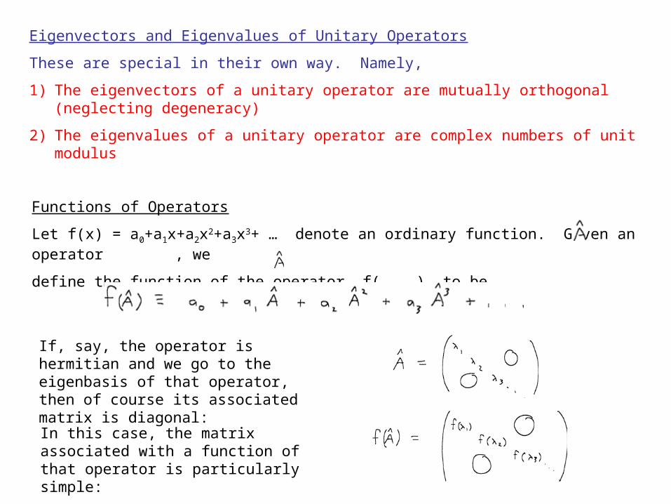
Eigenvectors and Eigenvalues of Unitary Operators
These are special in their own way. Namely,
1) The eigenvectors of a unitary operator are mutually orthogonal (neglecting degeneracy)
2) The eigenvalues of a unitary operator are complex numbers of unit modulus
Functions of Operators
Let f(x) = a0+a1x+a2x2+a3x3+ … denote an ordinary function. Given an operator , we
define the function of the operator, f( ), to be
If, say, the operator is hermitian and we go to the eigenbasis of that operator, then of course its associated matrix is diagonal:
In this case, the matrix associated with a function of that operator is particularly simple:
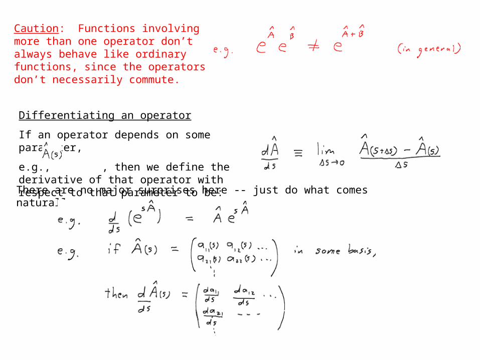
Caution: Functions involving more than one operator don’t always behave like ordinary functions, since the operators don’t necessarily commute.
Differentiating an operator
If an operator depends on some parameter,
e.g., , then we define the derivative of that operator with respect to that parameter to be:
There are no major surprises here -- just do what comes naturally:
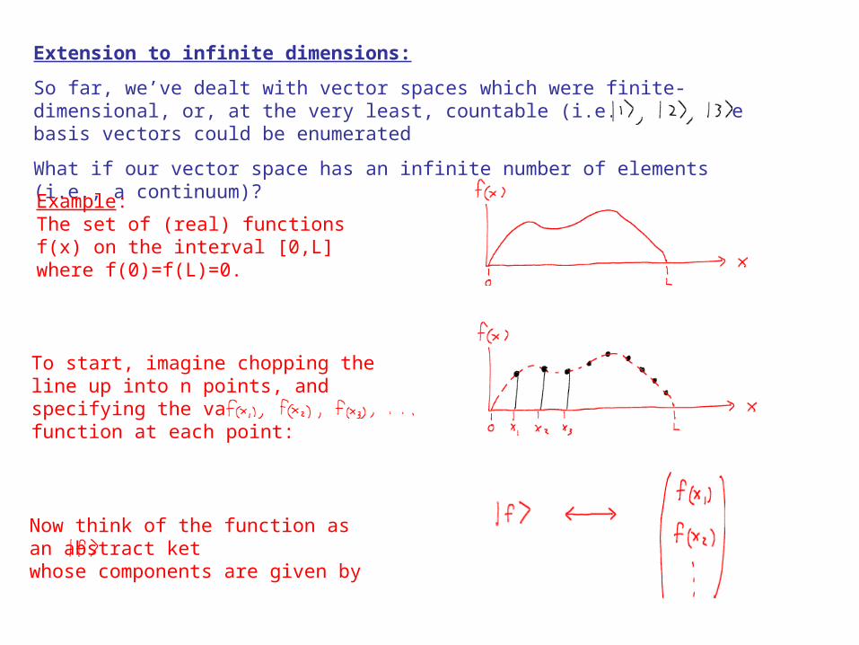
Extension to infinite dimensions:
So far, we’ve dealt with vector spaces which were finite-dimensional, or, at the very least, countable (i.e., where the basis vectors could be enumerated
What if our vector space has an infinite number of elements (i.e., a continuum)?
Example: The set of (real) functions f(x) on the interval [0,L] where f(0)=f(L)=0.
To start, imagine chopping the line up into n points, and specifying the value of the function at each point:
Now think of the function as an abstract ket whose components are given by
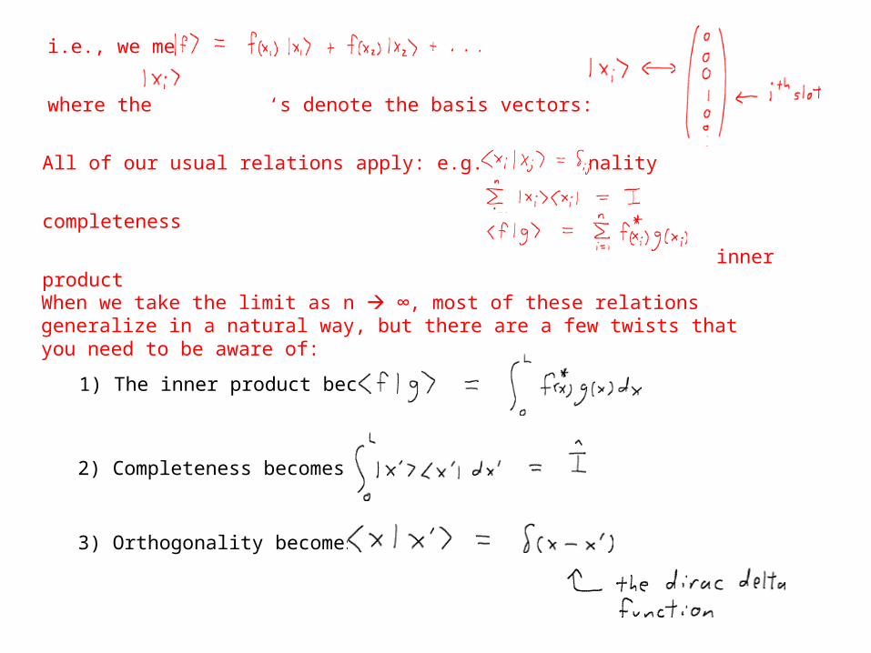
i.e., we mean
where the ‘s denote the basis vectors:
When we take the limit as n ∞, most of these relations generalize in a natural way, but there are a few twists that you need to be aware of:
All of our usual relations apply: e.g., orthogonality
completeness
inner product
1) The inner product becomes
2) Completeness becomes
3) Orthogonality becomes
Remarks
First, recall the meaning of the dirac delta function appearing in the orthogonality relation. By definition,
Using this definition, you can prove a many key facts, e.g., (see Shankar or Griffiths for details)
So the orthogonality condition tells that while the inner product between different kets is zero (as expected), the inner product of a ket with itself <x|x> is, somewhat surprisingly, infinite! This is a common feature of basis vectors in infinite-dimensional vector spaces – the length of the vectors is infinite (i.e., they are “non-normalizable”).
The non-normalizability is slightly annoying, but we’ll learn how to handle it – the key concepts we learned for finite-dimensional spaces remain intact.
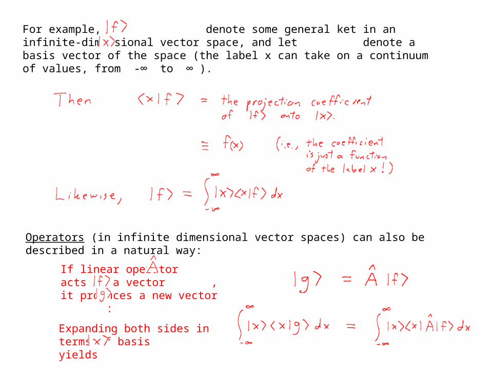
For example, let denote some general ket in an infinite-dimensional vector space, and let denote a basis vector of the space (the label x can take on a continuum of values, from -∞ to ∞ ).
Operators (in infinite dimensional vector spaces) can also be described in a natural way:
If linear operator acts on a vector , it produces a new vector :
Expanding both sides in terms of basis yields
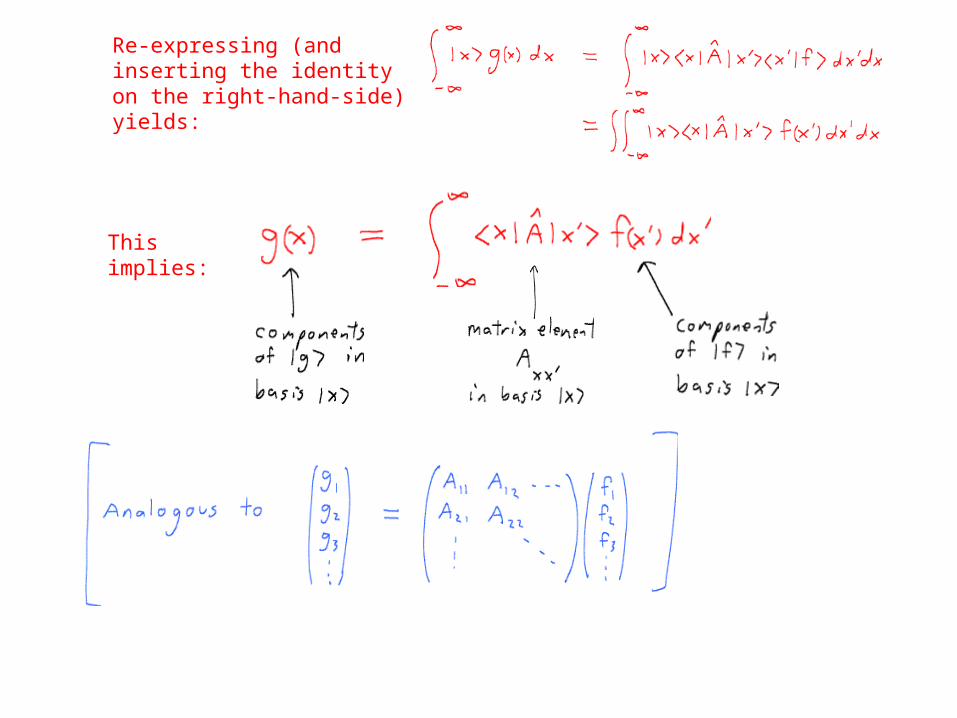
Re-expressing (and inserting the identity on the right-hand-side) yields:
This implies:
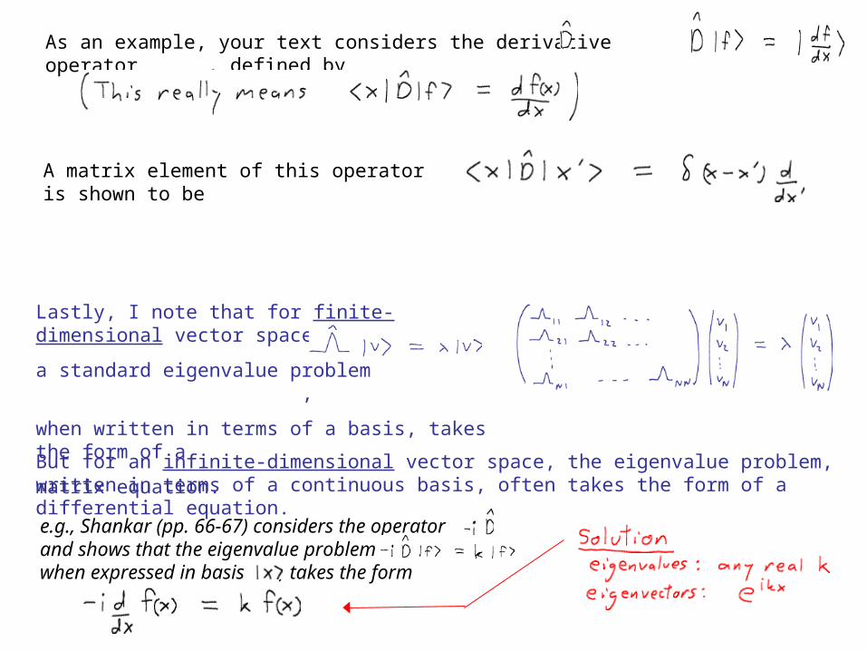
As an example, your text considers the derivative operator , defined by
A matrix element of this operator is shown to be
Lastly, I note that for finite-dimensional vector spaces,
a standard eigenvalue problem ,
when written in terms of a basis, takes the form of a
matrix equation.
But for an infinite-dimensional vector space, the eigenvalue problem, written in terms of a continuous basis, often takes the form of a differential equation.
e.g., Shankar (pp. 66-67) considers the operator , and shows that the eigenvalue problem , when expressed in basis , takes the form


![Quantum Mechanics relativistic quantum mechanics (RQM) · Quantum Mechanics_ relativistic quantum mechanics (RQM) ... [2] A postulate of quantum mechanics is that the time evolution](https://static.documents.pub/doc/80x56/5b6dfe707f8b9aed178e053e/quantum-mechanics-relativistic-quantum-mechanics-rqm-quantum-mechanics-relativistic.jpg)


