29
The MATLAB Reservoir Simulation Toolbox B˚ ard Skaflestad SIAM Geosciences, Long Beach, March 21–24, 2011

The MATLAB Reservoir Simulation Toolbox
Bard Skaflestad
SIAM Geosciences, Long Beach, March 21–24, 2011
The Matlab Reservoir Simulation Toolbox (MRST)
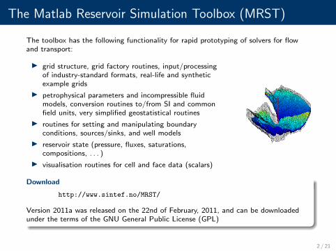
The toolbox has the following functionality for rapid prototyping of solvers for flowand transport:
I grid structure, grid factory routines, input/processingof industry-standard formats, real-life and syntheticexample grids
I petrophysical parameters and incompressible fluidmodels, conversion routines to/from SI and commonfield units, very simplified geostatistical routines
I routines for setting and manipulating boundaryconditions, sources/sinks, and well models
I reservoir state (pressure, fluxes, saturations,compositions, . . . )
I visualisation routines for cell and face data (scalars)
Download
http://www.sintef.no/MRST/
Version 2011a was released on the 22nd of February, 2011, and can be downloadedunder the terms of the GNU General Public License (GPL)
2 / 21
Software goals
I General framework for flow and transport in porous media
I Special focus on unstructured grids and multiscale methods
Research:
I Development of new solvers and discretization schemes
I Application to new scientific/engineering problems
I Preserve know-how and promote reuse of results from previous research
I Contribute to accelerating production of new research (by our peers)
I Benchmarking – compare different methods on standard test problems
Students:
I Develop students’ intuition of porous media flow
I Make it easy to test, compare, and extend existing methods
I Textbook (with worked examples) in preparation
3 / 21

Why open-source and why in Matlab?
First of all, prototyping in a scripting language is much more effective than intraditional compiled languages (C/C++/FORTRAN)
I Explore alternative algorithms/implementations close to mathematics
I Gradually replace individual (or bottleneck) operations with acceleratededitions callable from matlab
I Direct access to matlab environment and prototype whilst developingreplacement components
I More experienced in Matlab/Octave than in e.g., Python,
Why free and open-source software:
I Research funded by Norwegian Research Council should be freely available
I Combined with publications: a means to collaborate and disseminateresults, while protecting IP rights
I Support reproducible research and promote replicability
4 / 21

How is MRST designed?
The fundamental object in MRST is the grid:
I Data structure for geometry and topology
I Several grid factory routines
I Input of industry-standard (proprietary) format(s)
Physical quantities defined as dynamic objects in matlab
I Properties of medium (φ, K, net-to-gross, . . . )
I Reservoir fluids (ρ, µ, kr, PVT, . . . )
I Driving forces (wells, boundary conditions, sources)
I Reservoir state (pressure, fluxes, saturations, etc)
All MRST operations accept, manipulate and produce objects of these types.
Physical quantities are assumed to be in SI units.
5 / 21
How is MRST designed?
MRST core
I routines for creating and manipulating grids and physical properties
I basic flow and transport solvers (sequential splitting) for incompressibleand immiscible flow
Functionality is stable and not expected to change in future releases
Modules
Similar to matlab’s toolboxes. Implements more advanced solvers and tools:
I adjoint methods, experimental multiscale, fractures, MPFA, upscaling
I black-oil models, three-phase flow, vertically integrated models, . . .
I streamlines, (flow-based) coarsening, . . .
I Octave support, C-acceleration, . . .
Some are stable. Some are constantly changing to support ongoing research.New modules initiated by others are much welcome
5 / 21

Grids in MRSTComplex reservoir geometries
Corner point: Tetrahedral: PEBI:
I Accurate modelling of features such as faults, fractures, or erosion requires gridsthat are flexible with respect to geometry.
I Industry-standard grids are often nonconforming and contain complex grid-cellconnectivities, as well as skewed and degenerate cells
I There is a trend towards unstructured grids with general polyhedral cells
I Standard discretization methods produce wrong results on skewed and roughcells condition numbers
I The representation of (un)structured grids affects the efficiency of numericalmethods
6 / 21

Grids in MRSTCell geometries are challenging from a discretization point-of-view
Skewed and deformed blocks:
Many faces:
Difficult geometries:
Non-matching cells:
Small interfaces:
(Very) high aspect ratios:
800× 800× 0.25 m
7 / 21

Grids in MRSTAll grids are assumed to be unstructured
Basic representation:
cells nodes faces
1
2
3
4
5
6
7
8
1
2
3
4
5
6
7
8
9
10
11
12
13
14
1
2
3
4
5
6
7
cells.faces = faces.nodes = faces.neighbors =1 10 1 1 0 21 8 1 2 2 31 7 2 1 3 52 1 2 3 5 02 2 3 1 6 22 5 3 4 0 63 3 4 1 1 33 7 4 7 4 13 2 5 2 6 44 8 5 3 1 84 12 6 2 8 54 9 6 6 4 75 3 7 3 7 85 4 7 4 0 75 11 8 36 9 8 56 6 9 36 5 9 67 13 10 47 14 10 5: : : :
Choices in grid representation guided by utility and convenience in low-order
finite-volume methods. Available geometric information typically limited to
centroids, normals, areas, and volumes
8 / 21

Grids in MRSTExamples of basic grid types
% Rectillinear griddx = 1−0.5∗cos((−1:0.1:1)∗pi);x = −1.15+0.1∗cumsum(dx);G = tensorGrid(x, sqrt(0:0.05:1));plotGrid(G);
% Extrude a standard MATLAB datasetload seamountg = triangleGrid([x(:) y (:)]);P = pebi(g);V = makeLayeredGrid(P, 5);plotGrid(V), view(−40, 60), axis off
% Make and read a simple Eclipse input filegrdecl = simpleGrdecl([20, 10, 5], 0.12)G = processGRDECL(grdecl);plotGrid(G,'FaceAlpha',0.8);plotFaces(G,find(G.faces.tag>0), 'FaceColor','red');view(40,40), axis off
9 / 21

Grids in MRSTExamples of flexible gridding strategies
Hybrid grid – areal grid consistingof the following components
– radially refined grid at wells
– Cartesian along boundary
– hexahedral in interior
– polyhedral transition cells
extruded to 3D along vertical lines
Hierarchical grid
– triangular cells adapted to acurved line
– extruded to 3D, with throwalong curved surface
– coarse grid constructed bycollecting cells from fine grid
9 / 21
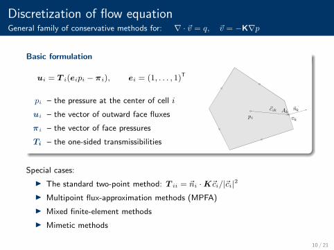
Discretization of flow equationGeneral family of conservative methods for: ∇ · ~v = q, ~v = −K∇p
Basic formulation
ui = T i(eipi − πi), ei = (1, . . . , 1)T
pi – the pressure at the center of cell i
ui – the vector of outward face fluxes
πi – the vector of face pressures
Ti – the one-sided transmissibilities
pi πk
Ak~cik
~nk
Special cases:
I The standard two-point method: T ii = ~ni ·K~ci/|~ci|2
I Multipoint flux-approximation methods (MPFA)
I Mixed finite-element methods
I Mimetic methods
10 / 21
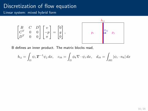
Discretization of flow equationLinear system: mixed hybrid form
24 B C DCT 0 0DT 0 0
3524 v−pπ
35 =
240g0
35 , vij
λij
pi pj
B defines an inner product. The matrix blocks read,
bij =
ZΩ
ψi T−1ψj dx, cik =
ZΩ
φk∇ · ψi dx, dik =
Z∂Ω
|ψi · nk| dx
Positive-definite system obtained by a Schur-complement reduction`DTB−1D − FTL−1F
´π = FTL−1g,
F = CTB−1D, L = CTB−1C.
Reconstruct cell pressures and fluxes by back-substition,
Lp = q + FTπ, Bv = Cp−Dπ.
11 / 21

Discretization of flow equationHerein: a mimetic method, Brezzi et al., 2005
Mu = (ep− π) ←→ u = T (ep− π)
Requiring exact solution of linear flow (p = xTa+ k):
MNK = C NK = TC
C – vectors from cell to face centroids. N – area-weighted normal vectors
Family of schemes (given by explicit formulas):
M =1
|Ωi|CK−1CT +Q⊥N
TSMQ
⊥N
T =1
|Ωi|NKNT +Q⊥C
TSQ⊥C
Q⊥N is an orthonormal basis for the null space of NT, and SM is any positive definite matrix. Herein, we usenull-space projection
P⊥N = Q
⊥N SM Q
⊥N = I −QN QN
T
12 / 21

Discretization of flow equationExample: grid orientation effects
Homogeneous domain with Dirichlet boundary conditions (left,right) andno-flow conditions (top, bottom) computed with three different pressure solversin MRST.
TPFA MFD MPFA
Homogeneous permeability with anisotropy ratio 1 : 1000 aligned with the grid.
100 × 100
13 / 21

Discretization of flow equationExample: lack of monotonicity
Homogeneous domain with Dirichlet boundary conditions (left,right) andno-flow conditions (top, bottom) computed with three different pressure solversin MRST.
TPFA MFD MPFA
Homogeneous permeability with anisotropy ratio 1 : 1000 rotated by π/6.
10 × 10
13 / 21

Application examplesA (very) simple flow solver
∇ · ~v = q, ~v = −K
µ
ˆ∇p+ ρg∇z
˜Vertical well and Dirichlet boundary
% Grid and rock parametersnx = 20; ny = 20; nz = 10;G = computeGeometry(cartGrid([nx, ny, nz]));rock.perm = repmat(100 ∗ milli∗darcy, [G.cells.num, 1]);fluid = initSingleFluid('mu', 1∗centi∗poise, ...
'rho' , 1014∗kilogram/meterˆ3);gravity reset on
% Fluid sources and boundary conditionsc = (nx/2∗ny+nx/2 : nx∗ny : nx∗ny∗nz) .';src = addSource([], c, ones(size(c)) ./ day());bc = pside([], G, 'LEFT', 10∗barsa());
% Construct components for mimetic systemS = computeMimeticIP(G, rock, 'Verbose', true);
% Solve the system and convert to barsrSol = initResSol(G, 0);rSol = solveIncompFlow(rSol,G,S,fluid,'src',src,'bc' ,bc);p = convertTo(rSol.pressure(1:G.cells.num), barsa() );
From tutorial: simpleSRCandBC.m
Source term and boundarycondition
Pressure distribution
14 / 21

Application examplesModelling faults in consistent schemes
Faults modelled as internal boundaries,with internal jump conditions
u±f = Tf (π∓f − π±f )
Gives an extended hybrid system. Inaddition, method to convert TPFAmultipliers to fault transmissibility Tf
Water cuts from producer #1
1 2 3 4 5 60
0.1
0.2
0.3
0.4
0.5
without multiplier
with multiplier
+ = TPFA solution · = mimetic
0.1
1
10
100
1000
15 / 21
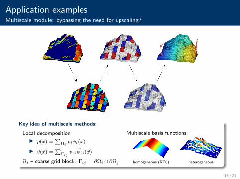
Application examplesMultiscale module: bypassing the need for upscaling?
Key idea of multiscale methods:
Local decomposition
I p(~x) =P
Ωipiφi(~x)
I ~v(~x) =P
Γijvij
~ψij(~x)
Ωi – coarse grid block. Γij = ∂Ωi ∩ ∂Ωj
Multiscale basis functions:
homogeneous (RT0) heterogeneous
16 / 21
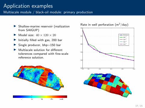
Application examplesMultiscale module / black-oil module: primary production
I Shallow-marine reservoir (realizationfrom SAIGUP)
I Model size: 40× 120× 20
I Initially filled with gas, 200 bar
I Single producer, bhp=150 bar
I Multiscale solution for differenttolerences compared with fine-scalereference solution.
Rate in well perforation (m3/day)
100 200 400 600 800 1000535
540
545
550
555
560
Reference
5⋅10−2
5⋅10−4
5⋅10−6
5⋅10−7
17 / 21
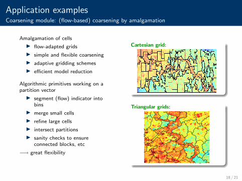
Application examplesCoarsening module: (flow-based) coarsening by amalgamation
Amalgamation of cells
I flow-adapted grids
I simple and flexible coarsening
I adaptive gridding schemes
I efficient model reduction
Algorithmic primitives working on apartition vector
I segment (flow) indicator intobins
I merge small cells
I refine large cells
I intersect partitions
I sanity checks to ensureconnected blocks, etc
−→ great flexibility
Cartesian grid:
Triangular grids:
18 / 21

Application examplesCoarsening module: (flow-based) coarsening by amalgamation
Dynamic adaption Different partitioning:
Adapting to geology
18 / 21
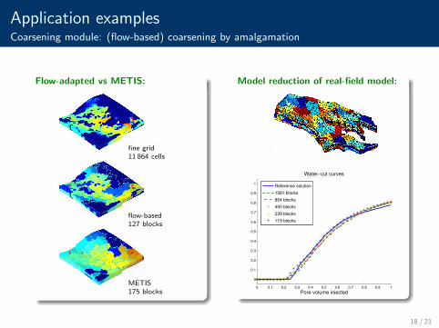
Application examplesCoarsening module: (flow-based) coarsening by amalgamation
Flow-adapted vs METIS:
fine grid11 864 cells
flow-based127 blocks
METIS175 blocks
Model reduction of real-field model:
0 0.1 0.2 0.3 0.4 0.5 0.6 0.7 0.8 0.9 1
0
0.1
0.2
0.3
0.4
0.5
0.6
0.7
0.8
0.9
1
Pore volume injected
Water−cut curves
Reference solution1581 blocks854 blocks450 blocks239 blocks119 blocks
18 / 21

Application examplesUpcoming adjoint module: production optimization
Specialized simulator: using differentgrids for pressure and transport
Multiscale pressure solver:
Transport on flow-adapted grid:
Water-flood optimization:
Reservoir geometry from a Norwegian Sea field
0 2 4 6 8 100
2
4
6
8
10
12
14x 10
6
Time [years]
Cum
.Pro
d. [m
3 ]
Oil initialOil optimizedWater initialWater optimized
Forward simulations:44 927 cells, 20 time steps, < 5 sec in Matlab
19 / 21

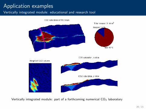
Application examplesVertically integrated module: educational and research tool
Vertically integrated module: part of a forthcoming numerical CO2 laboratory
20 / 21
Application examplesVertically integrated module: educational and research tool
Vertically integrated module: part of a forthcoming numerical CO2 laboratory
20 / 21

Application examplesVertically integrated module: educational and research tool
Vertically integrated module: part of a forthcoming numerical CO2 laboratory
20 / 21

Application examplesVertically integrated module: CO2 migration at Sleipner
3D model made by Statoil to study CO2 in the top layer of Utsira.MRST used to study physical assumptions and numerical methods:
I Simple to modify the code
I Flexible and simple upscaling (homogeneous model)
I Fast response time, simulation 2–10 min in Matlab
Seismic data (2006) / 3D simulation (tough2)
Fra: Chadwick, Noy, Arts & Eiken: Latest time-lapse seismic data from Sleipner yield newinsights into CO2 plume development, Energy Procedia (2009), 2103–2110.
VE simulation
21 / 21


