THE MATRIX OF CHROMATIC JOINS AND THE TEMPERLEY-LIEB ALGEBRA S.CAUTIS AND D.M.JACKSON Abstract. We show that the matrix of chromatic joins, that is associated with the revised Birkhoff- Lewis equations, can be expressed completely in terms of functions defined on a generalization of the Temperley-Lieb algebra. We give a self-contained account of the aspects of the Temperley-Lieb algebra that are essential to this context since these are not easily obtainable in this form. Of interest in the theory of these equations are recursions for the inverse of the matrix of chromatic joins. We show that the approach given here is a natural one which provides clear insight into the investigation of the properties of the inverse, and we give an instance of a recursion. It is hoped that these techniques will be of further value in the study of the revised Birkhoff-Lewis equations. 1. Introduction This paper is concerned with the study of the coefficient matrix L n (q), whose elements are monomials in an indeterminate q, for the revised system of Birkhoff-Lewis equations for the n-ring, discovered by Tutte [Tu1] that are associated with the Four Colour Problem. This matrix, whose size is exponential in n, has been termed the matrix of chromatic joins. Of interest in the theory of these equations are recursions for the elements of the inverse of this matrix. The value of the determinant has been obtained by Tutte [Tu2], verifying that L n (q) is generically invertible, and a recursion for the elements of the inverse has been obtained Dahab [D]. In fact, we shall study a more general matrix M n (x,y) which specializes to L n (q) through x = q and y =1. The primary purpose of this paper is to show that there is an enrichment TL n (x,y) of the Temperley-Lieb algebra TL n (q) that can be used to study recursions for the elements of the inverse of M n (x,y). We have used this algebra to derive such a recursion, and this is the main result (Thm 5.4) of the paper. The recursion involves only the cover relations of the distributive lattice L(P n , ≺ gi ) of Dyck paths in the plane ordered by geometrical inclusion (≺ gi ), with scalars that are are square roots of rational functions of generalized Chebyshev polynomials (in the indeterminates x and y). This strongly suggests that TL n (x,y) may be of further value in the examination of the revised Birkhoff-Lewis equations. Generalized Chebyshev polynomials in two indeterminates have also arisen independently in the work of Dahab [D] on the determinant of the chromatic join matrix, but for different reasons. The secondary purpose of this paper is to provide a self-contained and complete account of the aspects of TL n (x,y) that are relevant to this objective. We have used TL n (q) extensively and, where we have been unable to find complete proofs of the results that we require, we have supplied proofs which are extended to TL n (x,y). A number of the more technical proofs appear in the Appendix to avoid distraction from the main argument. We also remark that there is a close connexion between the present question and the classical problem of counting meanders, that is associated with Hilbert’s sixteenth problem, by specializing x Date : May 13, 2003. 1
Transcript
THE MATRIX OF CHROMATIC JOINS AND THE TEMPERLEY-LIEB
ALGEBRA
S.CAUTIS AND D.M.JACKSON
Abstract. We show that the matrix of chromatic joins, that is associated with the revised Birkhoff-Lewis equations, can be expressed completely in terms of functions defined on a generalization ofthe Temperley-Lieb algebra. We give a self-contained account of the aspects of the Temperley-Liebalgebra that are essential to this context since these are not easily obtainable in this form. Ofinterest in the theory of these equations are recursions for the inverse of the matrix of chromaticjoins. We show that the approach given here is a natural one which provides clear insight into theinvestigation of the properties of the inverse, and we give an instance of a recursion. It is hopedthat these techniques will be of further value in the study of the revised Birkhoff-Lewis equations.
1. Introduction
This paper is concerned with the study of the coefficient matrix Ln(q), whose elements aremonomials in an indeterminate q, for the revised system of Birkhoff-Lewis equations for the n-ring,discovered by Tutte [Tu1] that are associated with the Four Colour Problem. This matrix, whosesize is exponential in n, has been termed the matrix of chromatic joins. Of interest in the theoryof these equations are recursions for the elements of the inverse of this matrix. The value of thedeterminant has been obtained by Tutte [Tu2], verifying that Ln(q) is generically invertible, anda recursion for the elements of the inverse has been obtained Dahab [D]. In fact, we shall study amore general matrix Mn(x, y) which specializes to Ln(q) through x = q and y = 1.
The primary purpose of this paper is to show that there is an enrichment TLn(x, y) of theTemperley-Lieb algebra TLn(q) that can be used to study recursions for the elements of the inverseof Mn(x, y). We have used this algebra to derive such a recursion, and this is the main result(Thm 5.4) of the paper. The recursion involves only the cover relations of the distributive latticeL(Pn,≺gi) of Dyck paths in the plane ordered by geometrical inclusion (≺gi), with scalars that areare square roots of rational functions of generalized Chebyshev polynomials (in the indeterminatesx and y). This strongly suggests that TLn(x, y) may be of further value in the examination ofthe revised Birkhoff-Lewis equations. Generalized Chebyshev polynomials in two indeterminateshave also arisen independently in the work of Dahab [D] on the determinant of the chromatic joinmatrix, but for different reasons. The secondary purpose of this paper is to provide a self-containedand complete account of the aspects of TLn(x, y) that are relevant to this objective. We have usedTLn(q) extensively and, where we have been unable to find complete proofs of the results that werequire, we have supplied proofs which are extended to TLn(x, y). A number of the more technicalproofs appear in the Appendix to avoid distraction from the main argument.
We also remark that there is a close connexion between the present question and the classicalproblem of counting meanders, that is associated with Hilbert’s sixteenth problem, by specializing x
Date: May 13, 2003.
1
2 S.CAUTIS AND D.M.JACKSON
and y in the matrix Mn(x, y). For recent developments on meanders see [dF2]. The connexion withHilbert’s sixteenth problem is discussed by Arnol’d [A]. A brief account of the relevant backgroundto the Birkhoff-Lewis equations is now given to motivate the study of the inverse of the matrix ofchromatic joins.
We hope that the material on TLn(x, y) given here will lead to further progress on the revisedBirkhoff-Lewis equations.
1.1. Background to the Birkhoff-Lewis equations. Let M be a planar map bounded by acircuit J, with n vertices, such that each face of M within J is a triangle. J is called an n-ring. Thechromatic polynomial or chromial of M is a polynomial P (M, λ) in λ whose value is the number ofproper colourings of the vertices of M with λ colours. Details of the theory of chromials of planartriangulations, stated in the dual form, are given by Birkhoff and Lewis [BL]. The constrainedchromial on a partition π of the vertex set of J is the polynomial Q(M, π, λ) in λ whose valueis defined to be the number of ways of colouring M so that vertices of J have the same colour ifand only if they are in the same block of π. If T is a triangulation obtained from M by joiningvertices of π across the exterior face of M, then the chromial of T is called a free chromial of M.The Birkhoff-Lewis equations express each free chromial as a linear combination of constrainedchromials, consistent with the new edges. Birkhoff and Lewis then try to solve these equations, toexpress the constrained chromials in terms of the free chromials. They solved the equations for the5-ring and considered the 6-ring [BL]. Further information on the Four Colour Problem is givenin [SK].
Tutte [Tu2] has shown that the equations can also be obtained with the more relaxed conditionthat M be a triangulation and that the neighbouring elements on the n-ring be in distinct colourclasses. He derived his equations from the n-ring alone, without edges between neighbouringelements, with the aid of planar partitions. A non-planar partition of the vertex set of J is apartition such that two vertices of one block separate two vertices of another on J. The remainingpartitions are called planar. The chromatic join of a pair (π, γ) of planar partitions is the partitionwith the largest number of blocks that is refined by both of the partitions. The number of blocks inthe chromatic join is denoted by χ(π, γ). Tutte [Tu2] has shown that the Birkhoff-Lewis equationsare recoverable through the inverse of
Ln(q) =[
qχ(π,γ)]
l(n)×l(n),(1)
the matrix of chromatic joins, where l(n) is the number of planar partitions of J. Planar and non-planar partitions are also called, respectively, non-crossing and crossing partitions, and have beenstudied extensively (see [E], for example).
1.2. Connexion with TLn(x, y). The idea behind the paper is to use a combinatorial correspon-dence to express planar partitions of {1, . . . , n} in terms of planar diagrams called strand diagrams,which themselves can be expressed as concatenations of irreducible strand diagrams. The lattercorrespond to the generators e1, . . . , en of TLn(x, y). The number χ(π, γ) of blocks in the chromaticjoin of π and γ can be obtained from their corresponding TLn(x, y) elements by means of a tracefunction. With this accomplished, we use TLn(x, y) to construct a particular linear basis to assistin a triangularization argument that expresses Mn in the form
Mn = (P−1n )tDnP
−1n ,(2)
THE MATRIX OF CHROMATIC JOINS AND THE TEMPERLEY-LIEB ALGEBRA 3
where Pn is upper triangular and invertible and Dn is diagonal. From this the inverse of Mn isreadily determined.
A connexion between the Four Colour Problem and TLn(q) has been observed by others, andhas been expressed, for example, by Kauffman and Thomas [KT] as a combinatorial word problemin this algebra. However, the Temperley-Lieb algebra occurs in an entirely different way in thispaper, through the use of planar partitions. The authors would like to credit di Francesco [dF1],and di Francesco, Golinelli and Guitter [dFGL] for describing the construction of the basis B2 ofTLn(q) and for indicating the central ideas behind the main results in Appendices B and C.3. Wehave made extensive use of these papers. For further information on the Temperley-Lieb algebrathe reader is directed to [BR, GdlHJ, KL].
1.3. Organization of the paper. In Section 2 planar partitions are associated with elements inTLn(x, y). The matrix of chromatic joins is then expressed as the Gram matrix of a bilinear formon TLn(x, y). In Sections 3 we give the construction of another basis for TLn(x, y) that is usedin the diagonalization of the bilinear form. In Section 4 we show that there is an ordering of thisbasis such that the change of basis matrix is triangular. In Section 5 we obtain a recursion forthe elements of Pn (Thm. 5.4) and give an example of its use in obtaining an element of P6. Thedeterminant of Mn(x, y) (Thm 5.7) is also given. The Appendices contains proofs of the moretechnical results that are needed together with examples.
2. Planar partitions and the Temperley-Lieb algebra
To make the connexion between planar partitions and elements of the Temperley-Lieb algebrawe use geometrical representations of planar partitions as arch diagrams and strand diagrams.The latter two diagrams are standard ones in the theory of TLn(q). To assist the discussion, wedemonstrate the action of the constructions on the two planar partitions π0 = {{1, 2, 6}, {3, 4}, {5}}and γ0 = {{1, 4}, {2, 3}, {5}, {6}}. Their chromatic join is {{1, 2, 3, 4, 6}, {5}}.
2.1. Planar partitions. Let π be a planar partition of {1, . . . , n}. Then π can be represented bydistributing n points equally spaced on the circumference of a circle oriented in clockwise sensein the plane, with one point on the circle distinguished. The circle is therefore rooted. We adoptthe convention that the points are labelled 1 to n starting from the root in clockwise order. If{i1, . . . , ij}< is a block of π, then edges {i1, i2}, . . . , {ij , i1} are drawn in the interior of the circleso that they intersect neither themselves nor the edges corresponding to other blocks. This definesl(π) finite and mutually disjoint regions since π is planar. Figure 1 gives such a representation ofπ0. The circle may be thought of as J and the points as the vertices in J, labelled clockwise from 1to n.
1
4
5
6
3
2
Figure 1. The planar partition π0, with implicit labelling and shading
4 S.CAUTIS AND D.M.JACKSON
The blocks of the chromatic join of π and γ are the vertex sets of the components of the graphconstructed by drawing the edges of γ in the exterior of the circle in the planar partition π. This
54
3
2
1
6
gives the construction of the chromatic join of π0 and γ0 from their diagrams, since the number ofshaded components is equal to the number of blocks in the chromatic join.
In the planar diagrams throughout this section the labelling of points and shading of regionsare redundant since they are derivable from the rooting, but they are included to assist in thedescriptions of the constructions. Also, the number of planar partitions of {1, . . . , n} is Cn =(2n
n
)
/(n + 1), a Catalan number (see Appendix C.2).
2.2. A bijection between planar partitions and arch diagrams. A planar partition π maybe represented by 2n points 1, 1′, . . . , n, n′ distributed at unit intervals along an infinite, directedbase line, drawn in the plane, together with non-intersecting semicircular arcs
{i′1, i2}, {i′2, i3}, . . . , {i′j−1, ij}, {i′j , i1}centred on the line and drawn on the same side of it. A semicircular arc is called an arch and thediagram is called an arch diagram. The construction is feasible since π is a planar partition, and isclearly reversible. In Figure 2 the regions corresponding to the blocks of π0 are shaded.
1 2’2 3 3’ 4 4’ 5 6 6’5’1’
Figure 2. The arch diagram of π0.
Let γ be a planar partition of {1, . . . , n}. If the arch diagram of γ is reflected in its base line, andthe points on the base line of this diagram are then identified with the points on the base line ofthe arch diagram of π, then the number of shaded regions in the resulting diagram is immediatelyidentified as χ(π, γ). Figure 3 shows that χ(π0, γ0) = 2 since there are two shaded regions in theresulting diagram each of which corresponds naturally to a block in the chromatic join of π and γ.
2.3. A bijection between arch diagrams and strand diagram. If n is even, the strand di-agram of π is obtained by cutting the base line of the arch diagram of π at the mid-point of thesegment [1, n′], and then rotating one of the semi-infinite line segments so that it is parallel to theother, with j and j′ opposite 2n − j and (2n − j)′, respectively, for j = 1, . . . , n. The arches are
THE MATRIX OF CHROMATIC JOINS AND THE TEMPERLEY-LIEB ALGEBRA 5
1 2’2 3 3’ 4 4’5 6 6’5’1’
1 1’ 2 2’ 3 6’65’54’43’
Figure 3. Calculation of χ(π0, γ0) from the arch diagrams of π0 and γ0.
smoothly transformed so that they do not intersect each other and are called strands. The diagramis given a direction, called its orientation, from the line containing 1 (the head of the diagram) tothe line containing 2n (the tail of the diagram). The orientation is indicated by an arrow. Thestrand diagram therefore has a top and a bottom. Furthermore, two strand diagrams are equivalentif one can be deformed into the other smoothly while keeping each the endpoints i and i′ fixed. Forexample, the arch diagram of π0 and the corresponding strand diagram, with shading to indicatethe blocks of the partition, is
This construction extends naturally to odd n, although attention has to be paid to the shading.For example, the strand diagram for the planar partition {{1, 2, 5}, {3}, {4}} is the same as theright hand diagram of the three immediately above, with the sole difference that the final strandin the right hand diagram is removed. Subsequent results hold uniformly across these two cases,and therefore will not be considered separately.
The following operations on strand diagrams will be useful. The strand diagram πt, obtainedfrom π by reversing its orientation, is called the transpose of π. The concatenation πγ of π with γis the strand diagram obtained by identifying the i-th point from the top in the tail of π with thei-th point from the top in the head of γ, deleting closed loops that may be formed, and assigningto it the orientation of π (or, equivalently, γ). The closure π of π is the planar diagram obtainedby joining the i-th point from the top in the tail of π with the i-th point from the top in the headof π, for all such points, with arcs that intersect neither themselves nor the strands of π and thatare drawn so that they appear at the bottom of the diagram. We will call such a diagram a loopdiagram. An example is given in Figure 4.
It is clear from the observation about the construction of the chromatic join that
χ(π, γ) = #{shaded regions in πγt }(3)
6 S.CAUTIS AND D.M.JACKSON
11’22’
3’3
44’
Figure 4. A strand diagram and its closure
(or, equivalently, #{shaded regions in γπt } since h is symmetric). The construction is illustratedbelow, where the diagrams on the left and right correspond to the planar partitions π0 and γ0,respectively.
11’22’33’
6’65’5
4 44’55’66’
4’
11’22’33’
These observations lead to the introduction of the following algebra in which χ(π, γ) will be seento be the value of an appropriately defined trace function on an element in the algebra.
2.4. The Temperley-Lieb algebra. Throughout, sans serif symbols are used to denote elementsof the Temperley-Lieb algebra.
Definition 2.1. The Temperley-Lieb algebra on n elements is a free additive algebra with multi-plicative generators 1, e1, · · · , en−1 subject to the relations
R1 e2i = qei for i = 1, . . . , n− 1,
R2 eiej = ejei if |i− j| > 1,R3 eiei±1ei = ei for i = 1, . . . , n− 1,
where the indeterminate q commutes with all the elements and 1 is the multiplicative identity.
It is readily seen that every strand diagram can be obtained by concatenating strand diagramsselected from
1 = e = ii
ni+1
i1
n
1
The product in TLn(q) respects the concatenation of diagrams, with the convention that closedloops formed in the concatenation are marked with the indeterminate q and then deleted. To showthis, it is necessary only to verify the assertion for the generators. The sequences
THE MATRIX OF CHROMATIC JOINS AND THE TEMPERLEY-LIEB ALGEBRA 7
i
ii i+1 i
j
=i iR1.
R2.
R3.
e e = = e e
j+1
i=i+1
j
e e e = =i
= ei+1i+2
= q e 2i+1
ie =
j i
of planar diagrams confirms this. The dimension of this algebra is therefore Cn, the number ofplanar partitions of {1, . . . , n}.
Each planar partition corresponds to a unique strand diagram and thence to a monomial ine1, . . . , en−1. The set of all such (distinct) monomials, modulo relations R2 and R3, is a linear basisof TLn(q) over C(q), and is denoted by B1. For example, B1 = (1, e1, e2, e1e2, e2e1) is a basis ofTL3(q). There is therefore a bijection between the set of all planar partitions of {1, . . . , n} and theelements of the basis B1.
There is a natural inclusion TLn(q) ⊂ TLn+1(q) via en = 0 in TLn+1(q), which will be importantin the inductive constructions. For strand diagrams, this inclusion corresponds to removing thestrand diagram for en in TLn+1(q) and then deleting the bottom strand from the strand diagramof ei ∈ TLn+1(q) for i = 0, . . . , n − 1.
Definition 2.2. A function trn : TLn(q) → C(q) that satisfies conditions (1) and (2) among
1. trn is a linear functional,2. trn(ab) = trn(ba) for all a, b ∈ TLn(q),
is called a trace. If, in addition, trk satisfies
3. trk(aek−1) = trk−1(a) whenever a ∈ 〈1, e1, . . . , ek−2〉 for k ≥ 1
then trk is called a Markov trace.
It is shown in Appendix A that if a Markov trace exists then it is unique up to a multiplicativefactor.
Let #loop(e) be the number of loops in the loop diagram corresponding to the closure of thestrand diagram of e ∈ TLn(q). Then
trn(e) = q#loop(e)
extends linearly to a trace function on TLn(q). To check this, it is enough to prove that thetrace properties hold for the generators. But this is straightforward. One contribution to thenumber of loops comes from concatenation, which is recorded through relation R1, and the othercontribution comes from the closure of the element. Condition (3) for the Markov trace is showndiagrammatically on Figure 5. Thus trn is a Markov trace.
8 S.CAUTIS AND D.M.JACKSON
en-1 e
12...n
.
.
e
12...n
12..n-1
n=
Figure 5. The Markov condition for the trace
2.5. The generalized Temperley-Lieb algebra. The chromatic join can be incorporated intothis setting through a refinement of the above trace. Let e be the Temperley-Lieb element cor-responding to π. Let #sh(e) and #ush(e) denote, respectively, the number of (finite) shaded andunshaded regions in the loop diagram of the closure of e. Then
#sh(e) + #ush(e) = #loop(e).(4)
We now show that
φn(e) = x#sh(e)y#ush(e).(5)
is a Markov trace on the following suitable generalization of TLn(q).
Definition 2.3. The generalized Temperley-Lieb algebra TLn(x, y) with trace is a free additivealgebra over C(x, y) with a trace function and with multiplicative generators 1, e1, · · · , en−1 subjectto relations
S1 e2i = xiei for i = 1, . . . n− 1, where xi = x if i is odd and xi = y if i is even,
S2 eiej = ejei if |i− j| > 1,S3 eiei±1ei = ei for i = 1, . . . , n− 1
where the indeterminates x and y commute with all the elements and 1 is the multiplicative identity.
The parity condition in S1 is forced since tr(ei−1ei+1) = tr(ei−1eiei+1ei−1) = xi−1tr(eiei+1ei−1)and, similarly, tr(ei−1ei+1) = tr(ei+1ei−1eiei+1) = xi+1tr(ei−1eiei+1), so equating these gives xi−1 =xi+1. Note also that the dimension of TLn(x, y) is equal to Cn and that TLn(q) = TLn(q, q). Thefollowing result is now easily checked.
Lemma 2.4. φn is a Markov trace on TLn(x, y).
We note that, from Lemma A.1, φn is unique up to a multiplicative factor. From (5), φn(e) =
x#sh(e) When y = 1, so this trace function counts the number of parts in the planar partition e.Moreover, from (4), it specializes to φn(e) = x#loop(e) when x = y, so this trace function also countsthe number of loops in the closure of e.
2.6. The matrix of chromatic joins. Since χ(π, γ) may be obtained through the construction
χ(π, γ) = #sh(πγt) on planar diagrams, we now complete the translation of the combinatorialquestion to the Temperley-Lieb algebra, by defining the transpose of an element of TLn(x, y) sothat it is consistent with this construction.
Definition 2.5. The transpose t : TLn(x, y) → TLn(x, y) satisfies
THE MATRIX OF CHROMATIC JOINS AND THE TEMPERLEY-LIEB ALGEBRA 9
(1) eti = ei for i = 1, 2, . . . , n− 1,
(2) (ef)t = ftet for all e, f ∈ TLn(x, y),(3) (λe + γf)t = λet + γft for all e, f ∈ TLn(x, y) and λ, µ ∈ C(x1, . . . , xn).
This is a symmetric bilinear form on TLn(x, y), and the matrix of chromatic joins is the Grammatrix
Mn(x, y) = [〈ai, aj〉n]Cn×Cn,(7)
of 〈·, ·〉n with respect to the standard ordered basis B1 = (a1, . . . aCn) of monomials in TLn(x, y).In particular, from (1), (3) and (5),
Ln = Mn(q, 1).(8)
For example, the Gram matrix of 〈·, ·〉n with respect to (1, e1, e2, e1e2, e2e1) of TL3(x, y) is
M3(x, y) =
x2y x2 xy x xx2 x3 x x2 x2
xy x xy2 xy xyx x2 xy x2y xx x2 xy x x2y
.
Later, another ordering of {1, e1, e2, e1e2, e2e1} will be used, and it will also be denoted by B1.At this point, however, there is no reason to prefer a particular ordering.
3. The basis B2
Hereinafter we work within TLn(x, y) to construct an ordered basis B2 of TLn(x, y) with respectto which Mn has the form given in (2). The relations S1, S2 and S3 will be used extensively,although explicit reference seldom will be made to them. In addition, it will be more convenient toprove certain of the algebraic results by constructions based on strand diagrams. This is permissiblesince, as observed earlier, strand diagrams with concatenation, transposition and closure provide acombinatorial presentation of TLn(x, y) with a Markov trace.
3.1. Some special elements in TLn(x, y). We begin with some observations about the construc-tion of the special elements, En, called the Jones-Wenzl projectors, for TLn(x, y) through an analogywith the symmetric group. It is known that TLn(x, x) is a quotient algebra of the Hecke algebra,which in turn is a generalization of the group algebra CSn of the symmetric group. The lattercan be represented as a free additive algebra with multiplicative generators 1, t1, . . . , tn−1 subjectto the relations
T1 t2i = 1 for i = 1, . . . , n− 1,T2 titj = tjti if |i− j| > 1,T3 titi+1ti = ti+1titi+1 for i = 1, . . . , n− 2,
where ti is the adjacent transposition (i, i+1). By setting ti = 1−ei and taking the quotient modulothe ideal generated by the elements eiei±1ei − ei we obtain TLn(2, 2). The relation eiei±1ei − ei = 0is equivalent to the relation titi+1ti = 1 − ti − ti+1 + titi+1 + ti+1ti and so TLn(2, 2) ∼= CSn/I
10 S.CAUTIS AND D.M.JACKSON
where I is the ideal generated by the elements 1 − ti − ti+1 − titi+1ti + titi+1 + ti+1ti. In thelanguage of classical representation theory this quotient corresponds to reducing CSn modulo therepresentations corresponding to Young tableaux with more than two rows. This is because theYoung symmetrizers of tableaux containing at least three rows are equal to zero when evaluatedmodulo the relations 1 − ti − ti+1 + titi+1 + ti+1ti = titi+1ti.
Recall also that the Young symmetrizer z corresponding to a tableau with only one columnsatisfies tiz = z = zti for i = 1, . . . , n − 1 which is equivalent to eiz = 0 = zei. Thus, in the nextsection we shall construct elements En ∈ TLn(x, y) such that eiEn = 0 = Enei. These elements willplay a role in TLn(x, y) analogous to that of the Young symmetrizers in CSn.
With the above comments in mind, we therefore seek En ∈ TLn(x, y) such that (i) Enei =0 = eiEn for all 1 ≤ i ≤ n − 1 and (ii) En − 1 ∈ 〈e1, e2, . . . , en−1〉. Now En − 1 is generated bye1, . . . en−1 so, from (i), En+1(En − 1) = 0 = (En − 1)En+1 so En+1En = En+1 = EnEn+1. ThenEnEn+1En = En+1En = En+1. Thus En+1 = EnFnEn for some Fn ∈ TLn+1(x, y). However, theonly monomials that may appear in Fn are 1 and en since, by (i), the others give no contributionto EnFnEn. Hence Fn = λn1 − µnen for some λn, µn ∈ C(x, y). Clearly, λn = 1 from (ii). Thus ifEn exists then it must satisfy En+1 = En(1 − µnen)En = En − µnEnenEn. The next result showsthat this recursion does yield idempotents satisfying the conditions and characterizes µn. Notethat TLn(q, q) is the Temperley-Lieb algebra TLn(q), and the En are known in this case as theJones-Wenzl projectors.
The above observations provide the motivation for the following lemma, whose proof is an ex-tension of the proof for TLn(q), and is included for completeness. In the statement of the lemma,condition 2 is redundant since 0 = En(En−1) by conditions 1 and 3 so E2
n = En. However, condition 2is retained since it is convenient to have it stated explicitly with the other two.
Lemma 3.1. There is a unique element En ∈ TLn(x, y) satisfying the conditions that
(1) En − 1 belongs to the algebra generated by e1, e2, . . . , en−1,(2) E2
n = En,(3) Enei = 0 = eiEn for 1 ≤ i ≤ n− 1.
Moreover,
En+1 = En − µnEnenEn(9)
for n ≥ 1 with E1 = 1, where µi satisfies
µi+1 = (xi+1 − µi)−1(10)
for i ≥ 0 with µ0 = 0.
Proof. We show that En+1 satisfies conditions 1, 2, 3 and (En+1en+1)2 = µ−1
n+1En+1en+1 under theinductive hypothesis that En does.
The result holds trivially for n = 1. Now En+1 − 1 = (En − 1) − µnEnenEn and is thereforegenerated by e1, . . . , en so condition 1 holds.
THE MATRIX OF CHROMATIC JOINS AND THE TEMPERLEY-LIEB ALGEBRA 11
Now from equation (9) we have E2n+1 = En − 2µnEnenEn +µ2
n(Enen)2En. But En − 1 is generatedby e1, e2, . . . , en−1 so En and en+1 commute. Then, from equation (9)
en+1En+1en+1 = en+1Enen+1 − µnen+1EnenEnen+1
= xn+1Enen+1 − µnEn(en+1enen+1)En
= xn+1Enen+1 − µnEnen+1 = µ−1n+1Enen+1.
where we had used the fact that Enen+1 = en+1En since En is generated by 〈e1, . . . , en−1〉. Multi-plying on the left by En+1 gives (En+1en+1)
2 = µ−1n+1En+1Enen+1. But, from equation (9), En+1En =
E2n − µnEnenE2
n = En+1 so (En+1en+1)2 = µ−1
n+1En+1en+1. Combining these, we conclude that
E2n+1 = En − 2µnEnenEn + µnEnenEn = En+1, from equation (9), so condition 2 holds.
From condition 3, by hypothesis and by equation (9), we have En+1ei = Enei−µn(Enen)(Enei) = 0for 1 ≤ i ≤ n− 1. Also En+1en = Enen − µn(Enen)2 = 0, so condition 3 holds.
Finally, from condition 3, (1−En)ei = ei = ei(1−Ei) for i ≤ i ≤ n− 1 in the ring 〈e1, . . . , en−1〉,so 1 − En is the multiplicative identity, which is necessarily unique, so En is unique. �
It follows from Lemma 3.1 that if Vi ≡ Vi(x, y) is written in the form
µi = Vi−1/Vi(11)
for i ≥ 1 then Vk satisfies the recurrence equation
Vk+1 = xk+1Vk − Vk−1(12)
for k ≥ 1 with V0(x, y) = 1 and V1(x, y) = x. Since this identifies Vk(q, q) is the normalized Cheby-shev polynomial Uk of the second kind, we regard Vi(x, y) as a generalized Chebyshev polynomial.The inverse relation is
Vk = (µ1 . . . µk)−1.(13)
The appearance of Chebyshev polynomials is not entirely surprising. Trivially, planar partitionsare in bijection with planted plane trees through duality, and the generating series for the numberof the latter with respect to non-root vertices satisfies the functional equation T = x(1 − T )−1.This generates a continued fraction whose k-th convergent has the form xQk/Qk+1 where Qk+1 =Qk−xQk−1 for k ≥ 1 and Q−1 = 0, Q0 = 1. This is easily transformed into the generating series forVk(x, x). The series xQk/Pk+1 counts planted plane trees with height at most k. The correspondingseries in x and y counts two-coloured trees, with height at most k, with respect to the number ofvertices of each colour.
Corollary 3.2. Etn = En.
Proof. Trivially, conditions 1,2 and 3 of Lemma 3.1 hold with En replaced with Etn. But such an
element is unique by Lemma 3.1, and the result follows. �
Corollary 3.3. For 1 ≤ k ≤ n− 1 there is a unique element E(k)n ∈ TLn(x, y) such that
(1) E(k)n − 1 belongs to the algebra generated by ek, ek+1, . . . , en−1,
(2) E(k)n E
(k)n = E
(k)n ,
(3) E(k)n ei = 0 = eiE
(k)n for k ≤ i ≤ n− 1,
where E(n)n = E
(n+1)n = 1 by convention.
12 S.CAUTIS AND D.M.JACKSON
Proof. This follows directly from above by considering TLn−k+1(x, y) and shifting indices i 7→i+ k − 1. �
Note that E(1)n = En.
It follows from Corollary 3.3 that the strand diagram of each monomial in E(n−h+1)n is obtained
from the strand diagram of the corresponding monomial in Eh ∈ TLh(x, y) by attaching n− h− 1
parallel strands at the top. Thus E(n−h+1)n has the same structure as Eh in TLn(x, y). Moreover,
E(n−h+1)n can therefore be obtained from Eh by the substitutions ei 7→ en−h+i for i = 1, . . . , h − 1,
where Eh is obtained from the recursion given in (9). Note that this substitution is a bijective ring
homomorphism. It is also useful to observe that E(h)n is obtained from En−h+1 by
ei 7→ eh+i−1 and xi 7→ xh+i−1 for i = 1, . . . n− h.(14)
3.2. Paths. A path p of length 2n is a sequence of points (P0, . . . , P2n) in R2, such that P0 = (0, 0)
and Pi − Pi−1 = (1,±1) for i = 1, . . . , 2n. Let Pn denote the set of all such paths with P2n = (0, 0)and such that no point has negative y-coordinate. This is the set of Dyck paths. It is convenientto connect Pi−1 and Pi by an edge for i = 1, . . . , 2n.
The height, hi(p), of p is the y-coordinate of Pi. Then p has a rise at position i if hi+1(p) > hi(p),and a fall at position i if hi+1(p) < hi(p). Also, p has a minimum in position i if hi−1(p) = hi+1(p) =hi(p) + 1. Similarly, p has a maximum in position i if hi−1(p) = hi+1(p) = hi(p) − 1. In addition, p
has a double rise in position i if hi−1(p) + 1 = hi(p) = hi+1(p)− 1, and a double fall in position i ifhi−1(p)− 1 = hi(p) = hi+1(p) + 1. We say that p has a slope in position i if there is either a doublerise or a double fall in position i. Note that if a maximum or minimum occurs in position i andheight m then i ≡ m mod 2.
The steps (1, 1) and (1,−1) are called, respectively, a rise ր and a fall ց. A path in Pn cantherefore be regarded as sequence of rises and falls, starting at the origin, with no point below the x-axis. Given a path, the corresponding arch diagram is constructed by first associating the step (1, 1),with the beginning of an arch and the step (1,−1), with the end of an arch and then completingthis uniquely to an arch diagram. The correspondence is clearly bijective. Here and throughout,paths are denoted by Gothic minuscules. Figure 6 shows the path diagram ր2ցր3ց2րց3∈ P6
and its corresponding arch diagram.
321 11 120 2 2’3 3’ 4 4’1’1 6’ 65’5
Figure 6. A path and the corresponding arch diagram
Combining the above bijection with those from Section 2 gives a bijection
(·)1 : Pn∼→ B1
between Pn and B1, which is a basis of both TLn(q) and TLn(x, y),
THE MATRIX OF CHROMATIC JOINS AND THE TEMPERLEY-LIEB ALGEBRA 13
The path corresponding to a monomial a ∈ B1 is denoted by [a]. In this notation therefore[e2
i ] = [ei]. Also, if a is any monomial, then ([a])1 is the element in B1 that is equal to it. For brevitywe shall use [a]1 to denote ([a])1. In particular, if a ∈ B1 then [a]1 = a.
Finally, we shall need the transpose of a path. If s denotes a step define st =ր if s =ց andst =ց if s =ր (ie. st denotes the step complement of s). If p = s1 · · · sk where s1, . . . , sk are steps,then st
k · · · st1 is called the transpose of p and is denoted by pt. Thus pt is obtained from p by reading
the latter backwards and then specifying (0, 0) to be its origin. If r and l are paths, let δr,l = 1 ifl = r and 0 otherwise.
3.3. Box addition on paths. If p ∈ Pn has a minimum at position i, let p⊞ ⋄i denote the pathobtained combinatorially by complementing the steps incident with position i to make a maximumat position i. We can notionally regard p⊞⋄i as having been obtained from p by “adding a box” ⋄i atthe minimum in position i in p, and we shall refer to this operation as box addition. The operationis undefined if p does not have a minimum at position i. The reverse operation will be useful. Ifp ∈ Pn has a maximum at position i then p⊟ ⋄i denotes the path obtained by complementing thesteps incident with position i to make a minimum in position i. We can regard this operation as boxdeletion. It is easily verified that the basis B1 of monomials may be obtained through box additionby means of the following algorithm, in which
Ikn = (րց)j
(
րkցk)
(րց)j ∈ Pn
where k + 2j = n and 0 ≤ k ≤ n. Such a path is called a base path.
Algorithm 3.4. Let the mapping (·)1 act on Pn by (Inn)1 = 1 and, for k < n, by
(Ikn)1 = e1e3 . . . en−k−1,
where n ≡ k mod 2. The rest of the mapping is defined iteratively by
(p⊞ ⋄i)1 =
ei(p)1 if i < n and p has a minimum at position i,(p)1e2n−i if i > n, and p has a minimum at position i,undefined if i = n
(15)
Then the basis B1 of TLn(x, y) is the set (Pn)1 of images of Pn under (·)1.
The construction is not defined for i = n since en 6∈ TLn(q), so a box cannot be added to themidpoint of a path. This observation is a crucial one since it explains the significance of the midpointof a path in Pn, which plays a key role in the later algebraic and combinatorial constructions.
The height of the midpoint of p ∈ Pn is called the mid-height of p and is denoted by h(p). Figure 7shows the determination of [b] = [e2e3]⊞ ⋄4 and [c] = [e2e3]⊞ ⋄8 in TL6(q). Every path in Pn withmid-height k can therefore be obtained, not necessarily uniquely, by means of (15) through boxaddition from the base path Ik
n where k ≡ n mod 2. The number of base paths in Pn is ⌊12(2n+1)⌋.
The path [I39]1 = e1e3e5 is given in Figure 8.
If p ∈ Pn and h(p) = h, then the number of box additions required in the construction of p fromIh
n using (15) is referred to as the number of boxes in p, and is denoted by #⋄(p). Thus, #⋄(Ihn) = 0.
This number will be used in some of the inductive proofs.
14 S.CAUTIS AND D.M.JACKSON
321 4 110 12
[c]=
321 4 110 12
[b]=
321 4 110 12
[a]=
Figure 7. Box addition in TL6(q).
Figure 8. The path I39 = [e1e3e5].
3.4. The construction of the basis B2. Another basis B2 is constructed in a similar way to B1,from the same set of base paths but with a revised action of box addition.
Definition 3.5. Let the mapping (·)2 act on Pn by (Inn)2 = 1 and, for k < n, by
(Ikn)2 = x−(n−k)/2E(n−k+1)
n e1e3 . . . en−k−1,(16)
where n ≡ k mod 2. The rest of the mapping is defined iteratively by
(p⊞ ⋄i)2 =
√
µj+1
µj(ei − µj1)(p)2 if i < n and p has a minimum at position i,
√
µj+1
µj(p)2(e2n−i − µj1) if i > n, and p has a minimum at position i,
undefined if i = n
where j = hi(p) + 1. Let B2 be the set (Pn)2 of images of Pn under (·)2.
Note that the ei’s for 1 ≤ i ≤ n − h − 1 commute with the E(n−k+1)n term in (Ik
n)2. Thisconstruction is well defined since ({[a]⊞ ⋄i}⊞ ⋄j)2 = ({[a]⊞ ⋄j}⊞ ⋄i)2 whenever |i− j| > 1 by S2.If a is a monomial, we denote ([a])2 by [a]2 for brevity.
For example, ([e2e3]⊞ ⋄3)2 =√
µ3
µ2(e3 − µ2)[e2e3]2 and ([e2e3]⊞ ⋄8)2 = [e2e3]2
√
µ4
µ3(e4 − µ3). For
brevity, here and subsequently, we replace µj1 by µj where the context permits.
Any path p ∈ Pn can be uniquely decomposed into p 7→ (l, r) where p = lr, and l and r arepaths of length n. We shall call lr the midpoint decomposition of p. The main result regarding theelements in B2 may now be stated.
Theorem 3.6. If [a] = lr and [a′] = l′r′ are midpoint decompositions, where a and a′ are monomialsin TLn(x, y), then
[a]2[a′]2 = δrt,l′(lr
′)2.
THE MATRIX OF CHROMATIC JOINS AND THE TEMPERLEY-LIEB ALGEBRA 15
The proof of Theorem 3.6 is technical and so, to avoid interrupting the present development, itis deferred to Appendix B. The theorem shows that B2 is a semi-orthogonal basis for TLn(x, y)and it provides us with an easy way of multiplying elements of B2. Moreover, it gives the followingstructure theorem for TLn(x, y).
where Mi(C(x, y)) is the ring of i× i matrices over C(x, y) and ki =( n(n−i)/2
)
−( n(n−i−2)/2
)
.
Proof. We index the rows and columns of matrices in Mki(C(x, y)) by the paths of length n with
terminal height i. Consider map ψ given by (lrt)2 7→ e(h)l,r where h is the mid-height of the path
lrt ∈ Pn and e(h)l,r denotes the matrix in Mkh
(C(x, y)) with a 1 in position (l, r) and 0’s elsewhere.
The matrices from the other constituents are zero. Then, from Theorem 3.6, ψ is a homomorphismand a dimension argument proves that it is also bijective. Now ki is identified as the number ofpaths of length n with terminus at height i. The result follows from Lemma C.1, �
An example of the isomorphism is given in Appendix D.4.
Corollary 3.8. B2 is a basis of TLn(x, y).
Proof. Suppose that B2 is linearly dependent. Then there exist scalars αi ∈ C(x, y), i = 1, . . . , Cn,
not all zero, such that∑Cn
i=1 αi[ai]2 = 0. Assume that αk 6= 0. Let [ai] = liri be midpoint decompo-sitions for i = 1, . . . , Cn. Then, from Theorem 3.6,
0 = (lltk)2
(
Cn∑
i=1
αi(ai)2
)
(rtkr)2 =
Cn∑
i=1
αi(lkltk)2(liri)2(rtkrk)2 =
Cn∑
i=1
αiδli,lkδri,rk(liri)2 = αkak.
Thus αk = 0, which is a contradiction, so B2 is linearly independent. Finally, since dim(TLn(x, y)) =Cn = |B2| it follows B2 is a basis. �
It follows immediately that
(·)2 : Pn∼→ B2
is a bijection.
It is now possible to indicate informally the motivation behind the construction of basis B2
in Definition 3.5. Following the example of the symmetric group algebra, it is natural to obtainconstruct the elements of B2 recursively by multiplying left and right by selected factors. It remainsto justify why these factors should be ei−µj precisely when the corresponding path diagram containsa minimum at position i.
Suppose a factor contains a monomial e = ei1ei2 . . . eik . Then multiplying by e on the right isthe same as first multiplying by ei1 and then by ei2 and so on. So one may as well assume that themonomials are equal to ei for some i. Thus the factors ought to be polynomials in ei and since ei isidempotent each factor ought to have the form ei + c for some scalar c ∈ C(x, y). Now if the pathdiagram [a] has a slope at position i then [a]2(ei + c) = c[a]2 since, as is shown in Appendix B.1,[a]2ei = 0 if [a] has a slope at position i. Similarly if [a] has a maximum at position i then
[a]2(ei + c) ∼ [a′]2(ei − µj)(ei + c) ∼ [a′]2(ei + c′) ∼ [a]2 + [a′]2
16 S.CAUTIS AND D.M.JACKSON
where c′ ∈ C(x, y) and ∼ denotes that we have ignored scalar factors. This shows that multiplying[a]2 by ei + c has no effect if [a] has a maximum at position i. So to multiply by ei + c there oughtto be a minimum at position i in [a]. This justifies all the conditions in Definition 3.5 except whyc = µj. This can be deduced from the proofs of Theorem 3.6 in Appendix B where c must satisfya recursion enforced by the induction.
4. The matrix of chromatic joins
It is now possible to give a procedure for determining the elements of the inverse of the matrixLn of chromatic joins. We now show that the basis B2 is such that the Gram matrix of 〈·, ·〉 withrespect to it is diagonal. Moreover, we show that there is an ordering of the elements of B2 suchthat the matrix Pn that expresses the basis B2 in terms of B1 is a triangular matrix.
4.1. The Gram matrix. Some preliminary results on the evaluation of the Markov trace φn arerequired.
Lemma 4.1. (Ihn)2(I
h′
n )2 = δh,h′(Ihn)2.
The proof of this is given in Appendix B.1.
Lemma 4.2. φn(En) = Vn(x, y).
Proof. We use induction on n. If n = 1 then E1 = 1 and V1 = x = φ1(1). Now suppose thatφk−1(Ek−1) = Vk−1 for k < n. The lift of Ek−1 from TLk−1(x, y) to TLk(x, y) appends a strandto each of the strand diagrams, and therefore a region whose (implicit) shading is specified bythe parity of k. Then φk(Ek−1) = xkφk−1(Ek−1) = xkVk−1, by hypothesis. From (9) we haveφk(Ek) = xkVk−1 − µk−1φk(Ek−1ek−1Ek−1). But φk is a Markov trace and Ek−1 is idempotent, so
from (12) and the induction hypothesis. The result follows. �
We remark that this is another result in which the parity condition S1 of Definition 2.3 is required.
Lemma 4.3. φn((Ihn)2) = Vh whenever Ih
n exists (i.e. when n ≡ h mod 2).
Proof. Recall that (Ihn)2 = x−(n−h)/2E
(n−h+1)n e1e3 . . . en−h−1. But, from the remark following Corol-
lary 3.3, E(n−h+1)n has the same structure as Eh ∈ TLh(x, y). Now n−h+1 is odd so, by considering
the number of regions contributed by Eh, and the fact that each e2i+1 contributes a shaded region,it follows from the diagram
...
11’
n-h-1
hE
... ...
(n-h-1)’=nE e n-h-1
nn’
(n-h+1)3e 1e
that φn(E(n−h+1)n e1e3 . . . en−h−1) = x(n−h)/2φh(Eh), so φn((Ih
n)2) = φh(Eh) = Vh, from Lemma 4.2.�
THE MATRIX OF CHROMATIC JOINS AND THE TEMPERLEY-LIEB ALGEBRA 17
We may now give an explicit expression for the entries of the Gram matrix 〈·, ·〉n with respectto the basis B2.
Corollary 4.4. If a, a′ are monomials and [a] has mid-height h then
〈[a]2, [a′]2〉n = δa,a′Vh.
Proof. Let [a] = lr and [a′] = l′r′ be midpoint decompositions. Then, from (6) and Theorem 3.6,〈[a]2, [a′]2〉n = φn((lr)2(r
′l′)2) = δr,r′φn((ll′)2). Since the trace is invariant under a cyclic shift of itsargument, then 〈[a]2, [a′]2〉n = φn((r′l′)2(lr)2) = δl,l′φn((r′r)2). Thus 〈[a]2, [a′]2〉n = 0 if [a] 6= [a′].
In particular, 〈[a]2, [a]2〉n = φn((ll)2) and is therefore independent of r. Similarly, it is independentof l so it depends only on h and n. Therefore, 〈[a]2, [a]2〉n = 〈(Ih
n)2, (Ihn)2〉n = φn((Ih
n)2(Ihn)t2),
from (6). But (Ihn)t2 = (Ih
n)2 so, from Lemma 4.1, φn((Ihn)2(I
hn)t2) = φn((Ih
n)2) and the resultfollows from Lemma 4.3. �
Let Dn(x, y) be the matrix of 〈·, ·〉n with respect to the basis B2 = {[a]2 : i = 1, . . . , Cn} ofTLn(x, y). Let Pn be the matrix that expresses the elements of B2 in terms of the elements ofB1. Then Pt
nMn(x, y)Pn = Dn(x, y). Now Dn = [〈a, a′〉]a,a′∈TLn(x,y) so, from Corollary 4.4, Dn is
generically invertible. Thus Mn(x, y) is also. Moreover,
M−1n (x, y) = PnD
−1n (x, y)Pt
n.(17)
4.2. The change of basis matrix. We shall be able to select an ordering of B2 such that thechange of basis matrix Pn is a triangular matrix. This ordering will assist in the explicit deter-mination of elements of M−1
n (x, y). For this purpose, let L(Pn,≺gi) be the lattice of paths in Pn
where p1 ≺gi p2 (geometric inclusion) if p2 may be obtained from p1 by box additions.
Lemma 4.5. The basis B2 = {[ai]2 : i = 1, . . . , Cn} of TLn(x, y) has the property that
Proof. We use induction on #⋄(am). The base case is Ihn, where h is the mid-height of [am],
since #⋄(Ihn) = 0. Now (Ih
n)2 = x−(n−h)/2e1e3 . . . en−h−1E(n−h+1)n where E
(n−h+1)n is generated by
en−h+1, . . . , en−1. Thus every term in the expansion of (Ihn)2 has the form a = e1e3 · · · en−h−1f where
f ∈ 〈en−h+1, . . . , en−1〉. Now consider the concatenation of the strand diagrams of e1e3 . . . en−h−1
and f to obtain the product a. Since the last h strands of the strand diagram of e1e3 . . . en−h−1 arehorizontal and since f ∈ 〈en−h+1, . . . , en−1〉, concatenation with the strand diagram of f affects onlythese last h strands. So
[a] = [e1e3 . . . en−h−1f] = (րց)j p (րց)j
for some p ∈ Ph. But րhցh is the maximal element of the lattice L(Ph,≺gi) so p ≺giրhցh .Moreover,
[e1e3 . . . en−h−1] = Ihn = (րց)j (րhցh) (րց)j ,
where j is determined from n and h by n = h− 2j. It follows that [a] ≺gi Ihn. Thus
(Ihn)2 ∈ spanC(x,y)
{
a ∈ B1 : [a] ≺gi Ihn
}
,
establishing the base case.
18 S.CAUTIS AND D.M.JACKSON
Now consider b ∈ B1, where #⋄(b) > 0. As the inductive hypothesis we assume that the result istrue for all monomials with fewer than #⋄(b) boxes. Then [b] = [am]⊞⋄i for some i, so [am] ≺gi [b].We assume that i < n; the proof for the case i > n is similar and is therefore not included. Now
[b]2 = ([am]⊞ ⋄i)2 =√
µj+1
µj(ei − µj)am where j = hi([am]) + 1. Then, by hypothesis,
We now consider the expansion of eia. There are three cases, and in each of them we show that[eia] ≺gi [b] for each [eia] in the span.
Case I: Assume that [a] has a maximum in position i. Then [a] = [eif] for some f ∈ TLn(x, y).Thus [eia] = [e2
i f] = [eif] = [a] ≺gi [am] ≺gi [b], so [eia] ≺gi [b] in this case.
Case II: Assume that [a] has a minimum in position i. Then [eia] = [a]⊞ ⋄i ≺gi [am]⊞ ⋄i = b, so[eia] ≺gi [b] in this case.
Case III: Assume that [a] has a slope in position i. We assume that the slope is a double rise. Theproof for a double fall is similar and is therefore not included.
The arch diagram of a has two arches with heads in consecutive positions. In [a], these correspond
to risesi−1ր and
iր in positions i− 1 and i, together with matching falls
(i−1)
ց and(i)
ց, respectively(the bracketted index indicates the matching), corresponding to the ends of the two arches. Thus
[a] = ai−1ր(
iր b
(i)
ց)
c(i−1)
ց d
for some paths a, b, c, d. Now consider the concatenation of the strand diagram ei and the stranddiagram a. This affects precisely two strands in the strand diagram a, leaving all the other strandsuntouched. This is illustrated in Figure 9. It is immediately seen that the corresponding path is
...
...
...
...
...
...
...
...
...
...
xy
xy
z wwz
Figure 9. The strand diagram a on the left and eia on the right.
this next expression should be forced to appear before the diagram.
[eia] = ai−1ր(
iց b
(i)
ր)
c(i−1)
ց d.
Thus [eia] ≺gi [b] in this case. Combining these cases, we have
[b]2 ∈ spanC(x,y) {a ∈ B1 : [a] ≺gi [b]}so the inductive step holds, which completes the proof. �
We may now establish that Pn is triangular and obtain the elements on its diagonal. Thefollowing path statistic is needed. Let p ∈ Pn with p = lr its midpoint decomposition. Then the
THE MATRIX OF CHROMATIC JOINS AND THE TEMPERLEY-LIEB ALGEBRA 19
i-th fall in l marks a diagonal strip as does the j-th rise in r. In Figure 10 the shaded regions arethe strips of length three. Note that the strips have different orientations depending on whetherthey occur before or after the midpoint. This means that there are n − h strips in a path p ∈ Pn
with middle height h.
Figure 10. Strips of length 3 in path.
Corollary 4.6.
1) Pn is triangular,2) [Pn]k,k =
∏ni=1(
õi)
si,k ,
where si,k is the number of strips of length i in the path [ak].
Proof. 1) A linear extension of the lattice L(Pn,≺gi) can be constructed by shelling the lattice fromits top element. This shelling order gives a labelling a1, a2, . . . , aCn of the monomials of TLn(x, y)such that [ai] ≺gi [aj] ⇒ i < j. Let 1 ≤ m ≤ Cn. Then there exist γ1,m, γ2,m, . . . , γm,m ∈ C(x, y)together with a labelling of a1, . . . , aCn such that [am]2 =
∑mi=1 γi,mai. Thus Pn is triangular.
2) From Lemma 4.5, [Pn]k,k is equal to the coefficient of ak in the expansion of [ak]2 in the basis
B1. Suppose [ak] has mid-height h. We determine [ak]2 by box addition to Ihn to build [ak]. From
Definition 3.5, each box addition at height j−1 contributes a multiplicative factor√
µj
µj−1to [Pn]k,k.
A strip of length i therefore contributes a multiplicative factor√
Similarly, a possible ordering for B1 in L(P3,≺gi) is (e1, e2e1, e1e2, e2, 1). Then, by explicit compu-
tation, [e2e1]2 =√
µ2
µ1(e2 −µ1)µ1e1 =
√µ1µ2(−µ1e1 + e2e1) and it is noted that this is independent
of the elements e1e2, e2 and 1 in B1.
5. A recursion for the elements of M−1n (x, y)
We may now address the matter of constructing a recursion for the elements of M−1n (x, y), and
therefore, by specialization, a recursion for the elements of Ln(q). We propose to do this by first
20 S.CAUTIS AND D.M.JACKSON
obtaining a recursion for the elements of Pn, for then the elements of M−1n (x, y) may be obtained
through (17).
The determination of M−1n (x, y) has been reduced to the problem of expressing the basis B2 in
terms of the elements of B1. This, in principle, can be done through the recursive of Definition 3.5by means of box additions. However, the construction terminates on the base path Ik
n, whichcontains no boxes and, to complete the construction of B2, it would be necessary to use the difficult
non-linear recursion given in (9) for E(k)n . Recall that box additions cannot be made at the midpoint
of a path. We now show that it is possible to avoid this difficulty and to give a recursion for the
elements of B2 that operates uniformly down to the base path I0n or I
(1)n . To do this, we append a
particular fixed path to the paths p in Pn so the midpoint of p, at which box addition cannot becarried out, is no longer the midpoint. It is on the augmented path that the desired box additioncan be made. This means that we work in a left ideal of TL2n(x, y).
5.1. The ideal K2n(x, y). We begin by defining a natural map from TLn(x, y) to K2n(x, y) =TL2n(x, y)(e1e3 . . . e2n−1). This map is defined on monomials by e 7→ ([e] (րց)n)1, and extendedlinearly to TLn(x, y). Thus Γ(e) is the element of K2n(x, y) whose path is obtained from [a] by con-catenation on the right by (րց)n, the path corresponding to e1e3 . . . e2n−1. Clearly Γ is bijective.To simplify subsequent expressions we shall abuse notation slightly and denoted by Γ((p)1) by Γ(p)where p is a path.
Lemma 5.1. (1) Γ([a] + ⋄i) = Γ[a] + ⋄i for [a] ∈ Pn and 1 ≤ i ≤ 2n− 1.(2) Γ(eie) = eiΓ(e) for e ∈ TLn(x, y) and 1 ≤ i ≤ n− 1.(3) Γ(eei) = e2n−iΓ(e) for e ∈ TLn(x, y) and 1 ≤ i ≤ n− 1.
Proof. Part 1 follows immediately by considering box additions on paths. Parts 2 and 3 followimmediately by considering concatenation of strand diagrams. �
The next result shows that the basis B2 for TLn(x, y) and K2n(x, y) are directly related. Thiscorrespondence and the fact that box additions at position n in paths associated with K2n(x, y) areallowed will enable us to obtain a general recursion for all elements in the basis B2 of TLn(x, y)without resorting to the Ei’s.
Lemma 5.2. Let [a] ∈ Pn. Then
Γ([a]2) =√
xnVk[Γ([a])]2,
where k = h(a).
Proof. First note that [Γ(a)] is a path corresponding to a monomial in K2n(x, y). The correspond-ing B2 basis element [Γ([a])]2 is obtained by regarding K2n as a subset of TL2n(x, y). Then, byTheorem 4.5, the element [Γ([a])]2 belongs to K2n(x, y).
We will prove the result by induction on the number of boxes in [a]. The base case is [a] = Ikn
since #⋄(Ikn) = 0. Recall from (16) that (Ik
n)2 = x−(n−k)/2E(n−k+1)n e1e3 . . . en−k−1 where, from
Corollary 3.3, E(n−k+1)n is generated by en−k+1, . . . , en−1. Let
F = Γ−1(
(ΓIkn)2
)
,(18)
THE MATRIX OF CHROMATIC JOINS AND THE TEMPERLEY-LIEB ALGEBRA 21
so F ∈ TLn(x, y). Our intention is to show that F is equal to (Ikn)2, up to a multiplicative scalar in
C(x, y). Now if n− k + 1 ≤ i ≤ n− 1 then eiF = Γ−1(ei(Ikn)2) = Γ−1(0) = 0 since, by Lemma B.1,
Ikn has a slope in position i. Similarly Fei = 0 and thus
eiF = 0 = Fei for i = n− k + 1, . . . , n − 1.(19)
Moreover, from Lemma 4.5,
(ΓIkn)2 =
∑
e∈K2n(x,y)
[e]≺gi[ΓIkn]
βee
where βe ∈ C(x, y), so
F =∑
e∈K2n(x,y)
[e]≺gi[ΓIkn]
βeΓ−1e =
∑
e∈TLn(x,y)
[f]≺giIkn
βf f.
But Ikn = (րց)j(րkցk)(րց)j where 2j = n − k, so [f] = (րց)jp(րց)j where p ≺giրkցk .
Then F has the form F = β(e1e3 . . . en−k−1)F′, for some β ∈ C(x, y), where F′ − 1 is generated
by en−k+1, . . . , en−1, and where the 1 arises from the contribution to the sum from [f] = Ikn.
Then, from (19), 0 = eiF = β(e1e3 . . . en−k+1)(eiF′) so eiF
Then, by Corollary 3.3, F′ is unique so F′ = E(k)n . Thus F = β(e1e3 . . . en−k−1)E
(k)n = γ(Ik
n)2where γ ∈ C(x, y). Thus (ΓIk
n)2 = γΓ(
(Ikn)2)
. We determine γ by comparing the coefficients of
Γ(e1e3 . . . en−k−1) in (ΓIkn)2 and Γ
(
(Ikn)2)
.
In the construction of(
Γ(Ikn))
2, each box addition at height j contributes a factor of
√
µj+1/µ1
to the coefficient of Γ(e1e3 . . . en−k−1). This coefficient is equal to
µn1
√
µk
µ1
√
µk−1
µ1· · ·√
µ1
µ1=µ
n−k/21√Vk
,
by counting strips, using the argument in the proof of Corollary 4.6. Moreover, the coefficientof Γ(e1e3 . . . en−k−1) in Γ
(
(Ikn)2)
is equal to the coefficient of e1e3 . . . en−k−1 in (Ikn)2, which is
µ(n−k)/21 . Thus γ−1 =
√xnVk, and the base case of the induction is established.
For the inductive step, we assume that the result holds for [a], and we consider the addition ofa box at position i and height j in [a]. It will be assumed that i < n. The case i > n is similar andwill not be given. From Definition 3.5,
Γ (([a]⊞ ⋄i)2) =
√
µj+1
µjΓ ((ei − µj)[a]2)
=
√
µj+1
µj(ei − µj)Γ([a]2) (by Lemma 5.1)
=
√
µj+1
µj
√
xnVk (ei − µj)[Γ(a)]2
by the induction hypothesis. Thus, by Definition 3.5,
Γ (([a]⊞ ⋄i)2) =√
xnVk ([Γ(a)]⊞ ⋄i)2 =√
xnVk [Γ([a]⊞ ⋄i)]2
from Lemma 5.1. This completes the induction, and the result follows. �
22 S.CAUTIS AND D.M.JACKSON
The next example shows the use of Γ in constructing E2 in TL2(x, y) by box addition rather thanby the non-linear recursion given in (9).
Example 5.3. From Definition 3.5 we note that E2 = (I22)2. Then, by considering the concatenation
of paths, we have [ΓI22] = I0
4 ⊞ ⋄2, so (ΓI22)2 = (I0
4 ⊞ ⋄2)2. Thus
E2 = x√
V2 Γ−1(
(I04 ⊞ ⋄2)2
)
from Lemma 5.2. To evaluate this expression we work in TL4(x, y). From Definition 3.5, it follows
that (I04 ⊞ ⋄2)2 =
√
µ2/µ1 (e2 − µ1)(I04)2 where (I0
4)2 = x−2e1e3 from (16) and the convention ofCorollary 3.3. Thus
(I04 ⊞ ⋄2)2 = x−2
√
µ2
µ1(e2e1e3 − µ1e1e3).
To apply Γ−1, note that [e1e3] = (րց)2(րց)2 so [Γ−1(e1e3)] = (րց)2 = [e1] whence e1e3 =Γe1. Similarly, by path concatenation, [e2e1e3] = (ր2ց2)(րց)2 so [Γ−1(e2e1e3)] =ր2ց2= [1]
µ2/µ1(1− µ1e1). ButV0 = 1, V1 = x and V2 = xy − 1 from (11) and (12), so µ1 = x−1 and µ2 = x(xy − 1)−1. Therefore,
E2 = 1 − x−1e1.
This is, of course, in agreement with the recursion for the Jones-Wenzl projectors given in (9).
5.2. The recursion. We may now give a linear recursion for the elements of P−1n that operates
on paths by box addition in L(Pn,≺gi) using scalars from C(x, y). The following notation will beused for this purpose. Let p be a path in Pn with a double rise at position i. Then p has the form
p = ai−1ր(
iր b
(i)
ց)
c(i−1)
ց d
whereiր denotes a rise at position i and
(i)
ց denotes the matching step, soiր and
(i)
ց are associatedwith the same arch (the bracketted i indicates this pairing and not the position of the step). Thereis a similar form for p if it has a double fall at position i. So, if p has a slope at position i, let
κi(p) =
ai−1ր(
iց b
(i)
ր)
c(i−1)
ց d if p = ai−1ր(
iր b
(i)
ց)
c(i−1)
ց d
a(i)
ր b
(
(i−1)
ց ci−1ր)
iց d if p = a
(i)
ր b
(
(i−1)
ր ci−1ց)
iց d.
Thus κi(p) is obtained by collapsing p according to the type of step at position i. In the first casethe subpath b is ‘lowered’ by the complementation of the rise at position i and the matching step;in the second case the subpath c is ‘lowered’ by complementation of the fall at position i and thematching step. We shall call κi(p) the collapse of p at the slope at position i.
If q is a path in Pn with a slope at position i, let κ−1(q) denote the set of all paths p such thatκi(p) = q. For example, κ−1
3 ((րց)3) = {ր2ց2րց,րցր2ց2}.It is a straightforward matter to show, by carrying out the product through concatenation of
arch diagrams, that
[ei(p)1] = κi(p)(20)
where p has a slope at position i. We may now state the recursion for elements of Pn.
THE MATRIX OF CHROMATIC JOINS AND THE TEMPERLEY-LIEB ALGEBRA 23
Theorem 5.4. Let a, b ∈ Pn and let b have a minimum at position i. Then
[Pn]a,b⊞⋄i= −∆i,b
√µjµj+1 [Pn]a,b + δi,a∆i,b
√
µj+1
µj
xi[Pn]a,b + [Pn]a⊟⋄i,b +∑
e∈κ−1i
(a)
[Pn]e,b
where
δi,a =
{
1 if a has a maximum at position i,0 otherwise
, ∆i,b =
{ √
Vj+1
Vj−1if i = n,
1 if i 6= n,
and j = hi(b) + 1. The initial condition is
[Pn]a,b =
{
0 if a 6≺gi b,∏n
i=1
õi
si,a if a = b,
where si,a is the number of strips of length i in a.
Proof. If a, b ∈ Pn, and let [[(a)1]](b)2 denote the coefficient of (a)1 in (b)2. Therefore, in thisnotation, [Pn]a,b⊞⋄i
= [[(a)1]] (b⊞ ⋄i)2. From Lemma 5.2, for 1 ≤ i ≤ 2n− 1, we have Γ((b⊞ ⋄i)2) =√xnVk(Γ(b ⊞ ⋄i))2 where k = h(b ⊞ ⋄i). But, from Definition3.5, (Γ(b ⊞ ⋄i))2 =
√
µj+1/µj(ei −µj)(Γ(b))2 where j = hi(b) + 1 and, from Lemma 5.2, (Γ(b))2 =
√xnVk′Γ((b)2) where k′ = h(b).
Then
Γ((b ⊞ ⋄i)2) =
√
Vkµj+1
Vk′µj(ei − µj)Γ((b)2).
By considering the effect of box addition at position i = n, we have k = k′ + 2 if i = n and k = k′
otherwise so
(b⊞ ⋄i)2 = ∆i,b
√
µj+1
µj(ei − µj)(b)2.
Thus
[Pn]a,b⊞⋄i= ∆i,b
√
µj+1
µj[[(a)1]] ((ei − µj)(b)2) .(21)
There are two cases to be considered.
Case I: Suppose a does not have a maximum at position i. Since [ei(b)2] has a maximum at posi-tion i then [[(a)1]][ei(b)2] = 0 so the contribution to [Pn]a,b⊞⋄i
from this case is −∆i,b√µj+1µj [[(a)1]](b)2,
which is equal to
−∆i,b√µj+1µj [Pn]a,b.
Case II: Suppose a has a maximum at position i. Then, using part of the argument from case I,we see that the contribution to [Pn]a,b⊞⋄i
is
−∆i,b√µj+1µj [Pn]a,b + ∆i,b
√
µj+1
µj[[(a)1]][ei(b)2].
We now consider [[(a)1]][ei(b)2]. From Lemma 4.5, (b)2 =∑
[e]≺gibαee where αe ∈ C(x, y). Then
[[(a)1]] ei(b)2 =∑
[e]≺gib
[e] has max. at i
αe[[(a)1]] eie +∑
[e]≺gib
[e] has min. at i
αe[[(a)1]] eie +∑
[e]≺gib
[e] has slope at i
αe[[(a)1]] eie.
24 S.CAUTIS AND D.M.JACKSON
There are therefore three cases to be considered. First, suppose that [e] has a maximum at position i.Then e = eie
′ for some monomial e′ ∈ TLn(x, y). Thus eie = xieie′ = xie. For a contribution to
[[(a)1]] ei(b)2 it is necessary that (a)1 = eie = xie so a = [e]. Then [[(a)1]] eie = [[e]]xie = xi. Thus∑
[e]≺gib
[e] has max. at i
αe[[(a)1]] eie = xiαa = xi[Pn]a,b.
Next, suppose that [e] has a minimum at position i. For a contribution to [[(a)1]] ei(b)2 it is necessarythat [e] = a⊟ ⋄i. Then
∑
[e]≺gib
[e] has min. at i
αe[[(a)1]] eie = αa⊟⋄i= [Pn]a⊟⋄i,b.
Finally, suppose that [e] has a slope at position i. Then, from (20),∑
[e]≺gib
[e] has slope at i
αe[[(a)1]] eie =∑
[e]≺gib
[e] has slope at i
αe[[(a)1]] (κi([e]))1 =∑
[e]≺gib
[e]∈κ−1i
(a)
αe =∑
[e]≺gib
[e]∈κ−1i
(a)
[Pn][e],b.
The contribution to [P]a,b⊞⋄ifrom case II is therefore
∆i,b
√
µj+1
µj
xi[Pn]a,b + [Pn]a⊟⋄i,b +∑
e∈κ−1i (a)
[Pn]e,b
.
The recursion now follows by combining cases I and II by means of δi,a. The initial condition followsfrom Corollary 4.6. �
This is a linear recurrence equation with at most ⌊n/2⌋ + 2 terms and with coefficients that aresquare roots of rational functions of generalized Chebyshev polynomials. The k + 1-st column ofPn involves therefore at most ⌊n/2⌋ + 2 elements from the k-th column of Pn. Often there will bea position i at which b has a maximum and a does not. This will yield a recurrence equation withonly two terms.
5.3. Example: Computation of an element of P6. We conclude this discussion of the recursionwith a specific example of the computation of an element of P6, namely [P6]a,b, where
a =րրցրցրցրցցրց, b =րրրցրրցցրցցց .
This will require several invocations of the recursion given in Theorem 5.4. To simplify the discus-
sion,i= will be used to indicate an equality between two expressions that follows immediately from
the use of the recursion at position i. In addition, p⊟⋄k1k2...krdenotes p⊟⋄k1 ⊟ · · ·⊟⋄kr
, where theki’s are not necessarily distinct since there may be more than one box above position i in p. In theinterests of brevity, the determination of ∆i,b and δi,a at each stage are suppressed, but these arereadily checked by hand from the information that is provided. The strategy is to remove maximafrom b and to drive the recursion towards the boundary conditions. It is clear that the boxes inb\a, where a ≺gi b, play an important part in this calculation.
The path b has maxima in positions i = 3 and i = 9, and a does not have a maximum at thesepoints, so
[P6]a,b3= −√
µ2µ3 [P6]a,b⊟⋄3
9= µ2µ3 [P6]a,b⊟⋄3 9
.
THE MATRIX OF CHROMATIC JOINS AND THE TEMPERLEY-LIEB ALGEBRA 25
Since b⊟ ⋄3 9 has a maximum at position i = 10, and a does not have a maximum at this point,
[P6]a,b10= −µ2µ3
√µ1µ2 [P6]a,b⊟⋄3 9 10
Now b ⊟ ⋄3 9 10 has a maximum at i = 6, the midpoint of the path, and a also has a maximum atthis point. Moreover, a⊞ ⋄5 and a⊞ ⋄7 have a slope at i = 6, so κ−1
6 (a) = {a⊞ ⋄5, a⊞ ⋄7}. Then
[P6]a,b⊟⋄3 9 10
6= −
√
V4
V2
√µ3µ4 [P6]a,b⊟⋄3 9 10 6
+
√
V4
V2
√
µ4
µ3f
where
f = y[P6]a,b⊟⋄3 9 10 6+ [P6]a⊟⋄6,b⊟⋄3 9 10 6
+ [P6]a⊞⋄5,b⊟⋄3 9 10 6+ [P6]a⊞⋄7,b⊟⋄3 9 10 6
.
We now determine each of the four matrix elements in f. The path b ⊟ ⋄3 9 10 6, that appears ineach case, does not have maxima at i = 5 or i = 7. First, a does not have maxima at i = 5 or i = 7,so
[P6]a,b⊟⋄3 9 10 6
5= −√
µ2µ3 [P6]a,b⊟⋄3 9 10 6 5
7= µ2µ3 [P6]a,a = µ2µ3(µ
1/21 µ
3/22 ),
since b ⊟ ⋄3 9 10 6 5 7 = a. The last equality is by the boundary condition. Second, a ⊟ ⋄6 does nothave a maximum at i = 6, so
[P6]a⊟⋄6,b⊟⋄3 9 10 6
5= −√
µ2µ3 [P6]a⊟⋄6,b⊟⋄3 9 10 6 5
7= µ2µ3 [P6]a⊟⋄6,b⊟⋄3 9 10 6 5 7
6= −µ2µ3
√
V2
V0
√µ1µ2 [P6]a⊟⋄6,a⊟⋄6
= −µ2µ3
√
V2
V0
√µ1µ2 (µ
3/21 µ
3/22 ),
since b ⊟ ⋄3 9 10 6 5 7 6 = a ⊟ ⋄6, and the last equality is by the boundary condition. Thirdly, a ⊞ ⋄5
does not have a maximum at i = 7 so
[P6]a⊞⋄5,b⊟⋄3 9 10 6
7= −√
µ2µ3[P6]a⊞⋄5,a⊞⋄5= −√
µ2µ3(µ1/21 µ2µ
1/23 ),
since b⊟ ⋄3 9 10 6 7 = a⊞ ⋄5. The last equality is by the boundary condition. Finally, a⊞ ⋄7 does nothave a maximum at i = 5 so
[P6]a⊞⋄7,b⊟⋄3 9 10 6
5= −√
µ2µ3 [P6]a⊞⋄7,a⊞⋄7= −√
µ2µ3(µ1/21 µ2µ
1/23 ),
since b⊟ ⋄3 9 10 6 5 = a⊞ ⋄7. The last equality is by the boundary condition.
Combining these evaluations and using (10), we have
[P6]a,b = µ1µ32µ3 (µ2µ3 − yµ2 + µ1µ2 + 2) = µ1µ
32µ3 (1 + µ2µ3) .
5.4. Direct determination of [P6]a,b. To confirm the above calculation independently, we deter-mine [P6]a,b directly through the explicit computation of [[(a)1]](b)2 in TL6(x, y). Note that (a)1 =e2e1e4, by decomposing the strand diagram corresponding to a in terms of the strand diagrams ofthe generators of TL6(x, y). From (16) we have (I4
6)2 = x−1E36e1. Now e3(I
46)2 = (I4
6)2e3 = 0 fromLemma B.1, since I4
6 has a slope at position 3 so, from Definition 3.5,
From (14), E36 is obtained from E4 by the substitutions ei 7→ ei+2 and xi 7→ xi+2 for i = 1, 2, 3. Under
these transformations µi is unchanged since the displacement in i is even. Thus, from recursion (9)for Ei, we have E4 = E3 − µ3E3e3E3 where E3 = 1 − µ1(1 + µ1µ2)e1 − µ2e2 + µ1µ2e1e2 + µ1µ2e2e1.Then E3
6 = F3 − µ2F3e5F3 where F3 = 1 − µ1(1 + µ1µ2)e3 − µ2e4 + µ1µ2e3e4 + µ1µ2e4e3. We shallwrite p q, where p, q ∈ TL6(x, y), if [P6]a,b is unaffected by the replacement of p by q. We need
26 S.CAUTIS AND D.M.JACKSON
retain in F only terms having an occurrence of e4 and no occurrence of e5, since (a)1 = e2e1e4. Thisis because, in the formation of (b)2, E3
6 is multiplied on the left and the right by terms involvingonly e1, e2 and e3, and such terms do not lower the suffix of e5 and cannot introduce an e4. ThenF3e5F3 µ2
2e4e5e4 = µ22e4, so E3
6 −µ2(1 + µ2µ3)e4 + µ1µ2e3e4 + µ1µ2e4e3. Then
(b)2 −µ1µ22µ3e2E
36e1 µ1µ
32µ3(1 + µ2µ3)e2e1e4,
so [P6]a,b = µ1µ32µ3(1 + µ2µ3), in agreement with the result of the recursion.
5.5. The determinant of the Gram matrix. We conclude by confirming that detLn can nowbe determined. A preliminary result about path enumeration is needed for this purpose.
Proposition 5.5. Let bi be the total number of strips of length i in all the set of all paths in Pn.Let ci is the number of paths in Pn with mid-height at least i. Then
bi + ci =
(
2n
n− i
)
−(
2n
n− i− 1
)
.
The proof of this is given in Appendix C.
Theorem 5.6.
det(Mn(x, y)) =
n∏
i=1
Van,i
i where an,i =
(
2n
n− i
)
− 2
(
2n
n− i− 1
)
+
(
2n
n− i− 2
)
.
Proof. Let B2 now denote the ordered basis (a1, . . . , aCn) of TLn(x, y) such that [ai] ≺gi [aj] ⇒ i < jfor 1 ≤ i, j ≤ Cn. From (7), Mn(x, y) = [〈ai, aj〉n]Cn,Cn , the Gram matrix of 〈·, ·〉n with respectto B1. Let Dn = [〈[ai]2, [aj ]2〉n]Cn,Cn , the Gram matrix of 〈·, ·〉n with respect to B2 for TLn(x, y).Then Pt
nMn(x, y)Pn = Dn. Now from Corollary 4.4, 〈[ai]2, [aj ]2〉n = δi,jVh where h = h(ai), themid-height of [ai]. Then detDn =
∏nh=0 V
αh
h where αh is the number of paths in Pn with mid-height
exactly h. Thus, from (13), so detDn(x, y) =∏n
h=1 µ−ch
h where ch is the number of paths in Pn with
height at least h. Now from Corollary 4.6, detPn =∏Cn
h=1
∏ni=1
õi
si,k so (detPn)2 =∏n
i=1 µbi
iwhere bi is the number of strips of length i in the set of all paths in Pn. Then det(Mn(x, y)) =det(Pn)−2 det(Dn) =
∏ni=1(µi)
−bi−ci . The result follows from (11) and Proposition 5.5. �
We may now obtain the expression given by Tutte [Tu2] for the determinant of the matrix ofchromatic joins.
Theorem 5.7. The determinant of the chromatic join matrix is given by:
det(Ln) =n∏
i=1
Vi(q, 1)( 2n
n−i)−2( 2n
n−i−1)+( 2n
n−i−2).
Proof. In view of (8), the result follows from Theorem 5.6 by setting y = 1. �
The lattice of planar partitions is not closed under chromatic join so the evaluation of detLn
does not appear to be feasible through the lattice theoretic approach discussed by Jackson [J] fordeterminants of matrices of meets and joins in the lattice of partitions or the lattice of planarpartitions.
We note in passing that the number of occurrences of x in Mn(x, x) is the number of configu-rations of the type that appears in the right hand diagram in Figure 3, with the condition that
THE MATRIX OF CHROMATIC JOINS AND THE TEMPERLEY-LIEB ALGEBRA 27
there is a single loop (the indicated diagram has three loops). Such configurations are called closedmeanders, and they are the topic of extensive study. The number of closed meanders is thereforethe number of occurrences of the monomial x in Mn(x, x).
5.6. Closing remark. An important aspect of the recursion given in Theorem 5.4 is that, inprinciple, it gives a starting point for the further study of the matrix L−1
n (q). Although we havebeen unsuccessful in solving the recursion, it is clearly natural to ask whether the induced recursionfor the elements of L−1
n (q) = PnD−1n (q)Pt
n might have a solution. It appears that this is a questionfor which the incidence algebra of L(Pn,≺gi) is natural setting and that the properties of this latticewill be important to the investigation of this question.
References
[A] V.Arnol’d, The branched covering of CP2 → S4, hyperbolicity and projective topology, Siberian Math. J.,29 (1988), 717–726.
[BR] H.Barcelo and A.Ram, Combinatorial representation theory. In “New Perspectives in Algebraic Com-binatorics”, (eds. L.J.Billera, A, Bjorner, C.Greene, R.E.Simion and R.P.Stanley), Mathematical SciencesResearch Institute Publications 38, Cambridge University Press, Cambridge, England, 1999, pp. 23–90.
[BL] G.D.Birkhoff and D.C.Lewis, Chromatic polynomials, Trans. Amer. Math. Soc., 60 (1946), 355–451.[D] R.Dahab, “The Birkhoff-Lewis equations,” Ph.D. Thesis, Department of Combinatorics and Optimization,
University of Waterloo, Waterloo, Ontario, Canada, 1993.[E] P.Edelman, Chain enumeration and non-crossing partitions, Discrete Math., 31 (1980), 171–180.[dF1] P. di Francesco Meander determinants. hep-th/9612026.[dF2] P. di Francesco Folding and coloring problems in Mathematics and Physics, Bull. A.M.S. 37 (2000),
251–307.[dFGL] P. di Francesco, O.Golinelli and E.Guitter, Meanders and the Temperley-Lieb algebra, Commun.
Math. Phys., 186 (1997), 1–59.[GdlHJ] F.M.Goodman, P. de la Harpe and V.F.R.Jones, “Coxeter graphs and towers of algebra”, Mathemat-
ical Sciences Research Institute Publications 14, Springer, New York, 1989.[J] D.M.Jackson, The lattice of non-crossing partitions and the Birkhoff-Lewis equations, Europ. J. Combi-
natorics, 15 (1994), 245–250.[KL] L.H.Kauffman and S.Lins, “Temperley-Lieb Recoupling Theory and Invariants of 3-Manifolds”, Annals
of Mathematical Studies 134, Princeton University Press, New Jersey, 1994.[KT] L.Kauffman and R.Thomas, Temperley-Lieb algebras and the Four Colour Theorem. Available at
http://math.uic.edu/ kauffman/TLFCT.pdf.[SK] T.L.Saaty and P.C. Kainan, “The four colour problem,” Dover, New York, 1986.[Tu1] W.T.Tutte, On the Birkhoff-Lewis equations, Discrete Math., 92 (1991), 417–425.[Tu2] W.T.Tutte, The matrix of chromatic joins, J. Combinatorial Theory (B), 57 (1993), 269–288.
28 S.CAUTIS AND D.M.JACKSON
Appendix A. Uniqueness of the Markov trace
The following result shows that the Markov trace in TLk(x, y) is unique up to a multiplicativeconstant.
Lemma A.1. A Markov trace Trk in TLk(x, y) is uniquely determined by any one of its evaluations.
Proof. It is sufficient to prove the result for a monomial g. We may fix the evaluation of anymonomial so, for convenience, we fix Tr1(1). We show, using the relations (i) Trk(ef) = Trk(fe) and(ii) Trk(eek−1) = Trk−1(e) for e ∈ 〈1, e1, . . . , ek−2〉 from Definition 2.2, that Trk(g) can be reducedto Tr1(1). Suppose that g 6= 1. Then g = ej1 . . . ejl
for some integers j1, . . . , jl ∈ [1, k − 1]. Thestrategy is to use S3 of Definition 2.3 (viz. ei = eiei±1ei), to force the appearance of precisely oneek−1 and then, by (i), to move ek−1 to the end of g. We then use (ii) and repeat this procedure,terminating at the evaluation of Tr1(1). To do this, let M = max{j1, . . . , jl}. Then g = g1eMg2 forsome g1, g2 ∈ TLk(x, y). If M < k − 1 then
Since ek−1 has been forced to appear as the rightmost generator in g, we may suppose without lossof generality that M = k − 1.
If g now contains two ek−1’s, it is rewritten with them as close together as possible. If they areadjacent, e2
k−1 is replaced by xk−1ek−1, removing an ek−1. If not, g = · · · ek−1el1el2 · · · elsek−1 · · ·where l1 = k − 2 for otherwise we could use ek−1el1 = el1ek−1 to make the ek−1’s closer. Similarlyl2 = k − 3, . . . , ls = k − 1 − s. If s > 1 we commute els and ek−1, making the ek−1’s closer.Therefore, s = 1 and g = · · · ek−1ek−2ek−1 · · · = · · · ek−1 · · · , removing an ek−1. Repeating this, wemay assume that g contains exactly one ek−1. But then g = g′ek−1 where g′ ∈ 〈1, e1, . . . , ek−2〉 soTrk(g) = Trk−1(g
′) by (ii). Repeating this gives Trk(g) = Trk′(1) for some integer k′ ≥ 1. Finally,to determine Trk′(1), we have
Iterating this gives Trk′(1) = xk′−1xk′−2 . . . x1Tr1(1), so Trk(g) = xk′−1xk′−2 . . . x1Tr1(1). �
Appendix B. Inductive proof of Theorem 3.6
The main idea behind the determination of [a]2[a′]2 is to obtain a recurrence equation for it
by moving a box from r to l′, where lr and l′r′ are the midpoint decompositions of [a] and [a′],respectively. This idea leads to the statement of the theorem, which is now proved by an inductionthat is based on the recursion.
The base case of the induction is given in Appendix B.1 and the inductive step is given inAppendix B.2. Throughout, let
θj =
√
µj+1
µj.
THE MATRIX OF CHROMATIC JOINS AND THE TEMPERLEY-LIEB ALGEBRA 29
B.1. The base case of the induction.
Proof. (Lemma 4.1): For (Ihn)2 and (Ih′
n )2 to exist we require that n ≡ h mod 2 and n ≡ h′ mod 2,so h′ ≡ h mod 2. Now
(Ihn)2(I
h′
n )2 = x−(n−h)/2−(n−h′)/2(
E(n−h+1)n e1e3 . . . en−h−1
)(
E(n−h′+1)n e1e3 . . . en−h′−1
)
= 0
since en−h−1E(n−h′+1)n = 0 for h < h′ from Corollary 3.3. Similarly, by reorganizing the products,
(Ihn)2(I
h′
n )2 = x−(n−h)/2−(n−h′)/2(
e1e3 . . . en−h−1E(n−h+1)n
)(
E(n−h′+1)n en−h′−1 . . . e3e1
)
= 0
since E(n−h+1)n en−h′−1 = 0 for h > h′ from Corollary 3.3. Finally,
(Ihn)22 = x−(n−h)
(
E(n−h+1)n
)2e21e
23 . . . e
2n−h−1 = x−(n−h)/2E(n−h+1)
n e1e3 . . . en−h−1 = (Ihn)2,
since e2i = xei when i is odd and E
(n−h+1)n is idempotent. This gives the result. �
The base case of the induction corresponds to the case #⋄(r) = 0, and is established through thefollowing lemmas.
Lemma B.1. Let a be a monomial such that [a] has a slope at position i. Then
ei[a]2 = 0 if i < n,[a]2e2n−i = 0 if i > n.
Proof. We consider the case in which i < n and there is a double rise at position i in [a]. Since thethree other cases (i < n and double fall; i > n and double rise or double fall) are similar they arenot included.
We use induction on #⋄([a]). The base case of the induction is therefore Ihn where h is the
mid-height of [a]. Now Ihn has a double rise at position i, for n− h+ 1 ≤ i ≤ n− 1. But
ei(Ihn)2 = x−(n−h)/2eiE
(n−h+1)n e1e3 . . . en−h−1 = 0
by Corollary 3.3, so the result holds for [a] = Ihn.
We may now assume that Ihn ≺gi [a]. Let m− 1 be the height of the double rise at position i in
[a]. Then m−1 ≡ i mod 2. Now [a] is constructed by box additions ⋄i and ⋄i+1 either i) to a double
slope in the portion of [a] associated with E(n−h+1)n or ii) it is not. In case (i), the product is zero
by the inductive hypothesis. In case (ii), [a] is constructed by box additions ⋄i and ⋄i+1 to a pathg that therefore must have a double rise at position i+ 1. Thus, by box addition,
[a]2 = θm+1θmf(ei+1 − µm+1)(ei − µm)(g)2,
where g ≺gi [a]. Moreover, no paths corresponding to monomials in f have boxes in positions i− 1or i since [a] has a double rise in position i. Nor do these have a box in position i+ 1 since positioni+ 1 in [a] is not a minimum. Thus f is generated by {ej : |j − i| > 1}. Then eif = fei. Thus
But xi = xm+1 since m − 1 ≡ i mod 2, so ei[a]2 = −µm+1θm+1θmfeiei+1(g)2 from the recurrenceequation for µm. But ei+1(g)2 = 0 by the inductive hypothesis, and the result follows. �
30 S.CAUTIS AND D.M.JACKSON
Lemma B.2. Let a be a monomial, and let Ihn = lr and [a] = l′r′ be midpoint decompositions. Then
(Ihn)2[a]2 = δrt,l′(lr
′)2.
Proof. We use induction on #⋄(l′). Then the base case for the induction is [a] = Ih′
n , where h′ is
the mid-height of [a], since #⋄(l′) = 0. From Lemma 4.1, (Ihn)2[a]2 = (Ih
n)2(Ih′
n )2f = δh,h′(Ihn)2f =
δrt,l′(lr′)2, where f arises from the factors associated with box addition on the right of [a]. Thus the
result holds in this case.
We may now assume that #⋄(l′) > 0. Let i be a position in which a box appears and let j − 1be the height in this position at which the box addition takes place. Then j − 1 ≡ i mod 2, andi < n. There are two cases to consider.
Case I: Assume that i is odd. Now [a]2 = (([a]⊟ ⋄i)⊞ ⋄i)2 = θj(ei − µj)([a]⊟ ⋄i)2. Then
But i is odd, so [a]⊟ ⋄i contains at least two boxes (at positions i and i+1), so (Ihn)2([a]⊟ ⋄i)2 = 0
by the inductive hypothesis, whence (Ihn)2[a]2 = 0. Since #⋄(l′) > 0, then rt 6= l so δrt,l′(lr
′)2 = 0,
whence (Ihn)2[a]2 = δrt,l′(lr
′)2 so the inductive step holds in this case.
Case II: Assume that there is no such odd i. Then select the smallest even i such that the lastbox addition was at position i, to a point at height j − 1 where j ≥ 1. Then i ≡ j mod 2. Then[a] = ([a]⊟ ⋄i ⊟ ⋄i−1)⊞ ⋄i−1 ⊞ ⋄i so
[a]2 =
√
µj+1
µj−1(ei − µj)(ei−1 − µj−1)(p)2
where p = [a]⊟ ⋄i ⊟ ⋄i−1. Now
(Ihn)2[a]2 =
√
µj+1
µj−1x−(n−h)/2
(
E(n−h+1)n e1e3 . . . en−h−1
)
(ei − µj)(ei−1 − µj−1)(p)2.
But ei−1(ei − µj)(ei−1 − µj−1) = (1 − µjxi−1 + µjµj−1)ei−1 − µj−1ei−1ei = −µj−1ei−1ei from the
recurrence (10) for µj, since xi−1 = xj−1 for j ≡ i mod 2. Then (Ihn)2[a]2 = −√
µj+1µj−1 (Ihn)2ei(p)2.
But p has a double rise at position i so ei(p)2 = 0 by Lemma B.1. Thus (Ihn)2[a]2 = 0 = δrt,l′(lr
′)2.On the other hand, if j = 1 then µj−1 = 0 so (Ih
n)2[a]2 = 0 = δrt,l′(lr′)2. This establishes the
inductive step in this case. The result follows. �
The following is the base of the induction for the proof of Theorem 3.6.
Corollary B.3. Let r be the right factor of the midpoint decomposition of Ihn. Let [a] = lr and
[a′] = l′r′ be midpoint decompositions. Then
[a]2[a′]2 = δrt,l′(lr
′)2.
Proof. [a] can be constructed from Ihn by box additions ⋄i with i < n. By Definition 3.5 this
implies that [a]2 = b(Ihn)2 for some b ∈ TLn(x, y). Then [a]2[a
′]2 = b(Ihn)2[a
′]2 = δrt,l′(lr′)2 by
Lemma B.2. �
THE MATRIX OF CHROMATIC JOINS AND THE TEMPERLEY-LIEB ALGEBRA 31
B.2. The inductive step. We are now in a position to complete the proof of Theorem 3.6. Weconsider midpoint decompositions of paths p ∈ Pn and some further notation will be useful. Letp = λ(p)ρ(p) be the midpoint decomposition of p, and let λt(p) denote (λ(p))t. Thus pt = ρt(p)λt(p).Note that if p has a maximum, minimum or slope in position i > n, then ρ(p) has the same inposition i− n.
Proof. We begin by attaching the notation of the enunciation of the theorem: [a] and [a′] aremonomials in TLn(x, y), and [a] = lr and [a′] = l′r′ are midpoint decompositions. We use inductionon #⋄(r). The strategy for the inductive step is to consider the effect of moving a box from r to l′.The base case of the induction is for #⋄(r) = 0, and this is established immediately by Corollary B.3.
We may now assume that #⋄(r) > 0. Then there is a box in [a] at some position i > n, so[a] = [b]⊞ ⋄i where [b] has a minimum in position i, at height j − 1, say. Then
[a]2 = θj[b]2(e2n−i − µj)(22)
where i ≡ j − 1 mod 2. Then
[a]2[a′]2 = θj [b]2(e2n−i − µj)[a
′]2.
There are three cases.
Case I: Assume that [a′] has a minimum in position 2n − i < n, and at height k − 1, say. Then([a′]⊞ ⋄2n−i)2 = θk(e2n−i − µk)[a
′]2 so
[b]2([a′]⊞ ⋄2n−i)2 = θk[b]2(e2n−i − µk)[a
′]2.
But [b] has a minimum in position i and [a′]⊞⋄2n−i has a maximum in position 2n− i. Thus, by theinduction hypothesis, [b]2([a
′]+⋄2n−i)2 = 0 since #⋄([b]) < #⋄([a]). Then [b]2e2n−i[a′] = µk[b]2[a
′]2.Eliminating [b]2e2n−i[a
′] with this from the expression for [a]2[a′]2, we have
[a]2[a′]2 = θj(µk − µj)[b]2[a
′]2.
If ρ(b) = λt([a′]), then j = k since [b] and [a′] have minima at height j−1 and k−1, respectively.Thus µj = µk whence [a]2[a
′]2 = 0. On the other hand, if ρ([b]) 6= λt([a′]) then, by the inductionhypothesis, [b]2[a
′]2 = 0 so, again, [a]2[a′]2 = 0. But rt 6= l′ since [a] has a maximum in position
i and [a′] has a minimum in position 2n − i. Thus δrt,l′ = 0 whence [a]2[a′]2 = δrt,l′(lr
′)2, so theinductive step holds in this case.
Case II: Assume that [a′] has a slope in position 2n− i < n. Then
[a]2[a′]2 = θj [b]2(e2n−i − µj)[a
′]2.
But e2n−i[a′]2 = 0 by Lemma B.1, and [b]2[a
′]2 = 0 by the induction hypothesis, so [a]2[a′]2 = 0.
Moreover, δrt,l′ = 0, since rt has a maximum in position n− i, where l′ has a slope. Thus [a]2[a′]2 =
δrt,l′(lr′)2, so the inductive step holds in this case.
Case III: Assume that [a′] has a maximum in position 2n − i < n, at height k + 1, say. Then[a′] ⊟ ⋄2n−i has a minimum in position 2n − i at height k − 1. Now [a′] = [a′] ⊟ ⋄2n−i ⊞ ⋄2n−i so[a′]2 = θjθk(e2n−i − µk)([a
′]⊟ ⋄2n−i)2 so, from (22),
[a]2[a′]2 = θjθk[b]2(e2n−i − µj)(e2n−i − µk)([a
′]⊟ ⋄2n−i)2.
But (e2n−i −µj)(e2n−i −µk) = (x2n−i −µj −µk)(e2n−i −µk)+µk(x2n−i −µk). It follows from thesethree expressions that
[a]2[a′]2 = θj(x2n−i − µj − µk)[b]2[a
′]2 + θjθk µk(x2n−i − µk)[b]2([a′]⊟ ⋄2n−i)2
32 S.CAUTIS AND D.M.JACKSON
so
[a]2[a′]2 = θjθk µk(x2n−i − µk)[b]2([a
′]⊟ ⋄2n−i)2
since [b]2[a′]2 = 0 by the induction hypothesis.
Now [b] has a minimum in position i and [a′] ⊟ ⋄2n−i has a minimum in position 2n − i. Thusρ([b]) and λt([a′]⊟⋄2n−i) both have minima in position i−n. We now examine this situation. Thereare two cases.
i) If ρt([b]) 6= λ([a′]⊟ ⋄2n−i) then [b]2([a′]⊟ ⋄2n−i)2 = 0 by the induction hypothesis. But in this
case, rt 6= l so δrt,l′ = 0. Thus [a]2[a′]2 = δrt,l′(lr
′)2, so the inductive step holds in case (i).
ii) On the other hand, if ρ([b]) = λt([a′]⊟ ⋄2n−i) then [b]2([a′]⊟ ⋄2n−i)2 = (lr′)2 by the induction
hypothesis. Moreover, in this case j = k so, from (10),
[a]2[a′]2 = µj+1(x2n−i − µj)(lr
′)2 =x2n−i − µj
xj+1 − µj(lr′)2 = (lr′)2
since i ≡ j−1 mod 2. But ρt([b]) = λ([a′]⊟⋄2n−i) so rt = ρt([a]) = λ([a′]) = l′ so [a]2[a′]2 = δrt,l′(lr
′)2,so the inductive step holds in case (ii).
Thus the inductive step holds in case III. The result now follows. �
We note that this proof requires the parity condition in S1.
Appendix C. Paths
C.1. The lattice L(Pn,≺gi). Included in this Appendix are further facts about L(Pn,≺gi). Thelattice is graded and distributive. Its rank function rank(p) is given by the area (number of unitsquares) of the lattice polygon bounded by p ∈ Pn and the minimal element (րց)n. The numberrk,n of elements in L(Pn,≺gi) with rank equal to k is [ukxn]F0 where Fi satisfies the recursion
Fk = (1 − ukxFk+1)−1 for k ≥ 0. This generates the continued fraction of Ramanujan and it can
C.2. Enumeration of paths. The number of planar partitions of {1, . . . , n} is equal to the numberof arch diagrams on 2n points, and this is equal to the number of well formed brackets with n ofeach type. The set S of well formed brackets with the null bracket ε adjoined can be decomposed asS − {ε} ∼→ (S)S. The number of planar partitions of {1, . . . , n} is therefore the coefficient of xn in
S where S is the solution of S − 1 = xS2 with non-negative coefficients. This is Cn =(
2nn
)
/(n+ 1),a Catalan number.
Lemma C.1. The number of paths of length n with no point at negative height and with terminusat height i is
ki =
(
n12(n− i)
)
−(
n12(n− i− 2)
)
.
Proof. We use the the Reflexion Principle as follows. Consider the set of all paths from (0, 0) to(n, i). From this we wish to remove paths having a point at negative height, which are characterizedas those that cross the line y = −1. Such a path p may be written uniquely as p = ab where theterminus of a is the first point (from the left) in p with negative height. Let ar be the reflexion of a
in the line y = −1. Thus q = arb is a path from (0,−2) to (n, i). Then the mapping p 7→ q defines a
34 S.CAUTIS AND D.M.JACKSON
bijection between the set of all paths from (0, 0) to (n, i) with at least one point at negative heightand the set of all paths from (0,−2) to (n, i). Then ki = N((0, 0), (n, i)) −N((0,−2), (n, i)) whereN((a, b), (r, s)) be the number of paths from (a, b) to (r, s) where r ≥ a. But, trivially,
N((a, b), (r, s)) =
(
r − a12(r + s− a− b)
)
.
The result follows. �
C.3. Proof of Proposition 5.5. The proof given here is essentially a combination of proofs given
by di Francesco [dF1]. Let #jր(p, [r, s]) denote the number of rises at height j in p ∈ Pn in positions
r, . . . , s where r ≤ s. The corresponding number of falls is #jց(p, [r, s]).
Proof. A strip of length j in p ∈ Pn corresponds to a step in position i in p at height j, which is a fall
if 0 ≤ i ≤ n− i or a rise if n ≤ i ≤ 2n−1. But #jց(p, [0, n−1])+#j
ր(p, [n, 2n−1]) = #jց(p, [0, 2n−
1]) − ζ(j, p). where ζ(j, p) = 1 if j < h(p) and 0 otherwise. Now bj is the number of strips oflength j in the set of all paths in Pn, and is therefore equal to the number of paths in Pn with adistinguished strip of length j. Then bj = #{paths in Pn with a distinguished fall at height j}−cj ,so bj + cj = #{paths in Pn with a distinguished fall at height j}.
Let q be a path in Pn with a distinguished fall at height j. Then q can be factorized uniquelyinto q = lr where the distinguished fall is the last step of l. Then q′ = lrt is a path of length 2n withterminal height 2j and with no point at negative height. This construction is reversible since thedistinguished fall is the first fall from the right in q′ at height j, and this step is the terminal stepof l, thereby recovering the factorization. Thus bj + cj is the number of paths of length 2n withterminal height 2j and with no point at negative height. The result follows from Lemma C.1. �
Appendix D. The construction of the change of basis matrix B2 for TL3(x, y)
This appendix gives the construction of the bases B1 and B2 for TL3(x, y), the change of basismatrix P3 and D3 directly from the set of paths P3 using box addition.
D.1. Determining P3 and the box additions. The base paths are I13 and I3
3, that have mid-height 1 and 3, respectively. They are given by I1
3 = (րց)3 and I33 =ր3ց3 . The elements of P3
are constructed from these by box additions in increasing order of mid-height h and, within pathsof the same mid-height, in increasing order of #⋄. The box addition are to be used to determineB2. There are C3 = 5 paths to be constructed.
Below is a listing of the paths of P3 constructed in this order, each presented as a midpointdecomposition.
h #⋄ (posn., height) box additions path p in P3 [p]1 0 (2, 0), (4, 0) I1
3 (րցր)(ցրց) e1
1 1 (4, 0) I13 ⊞ ⋄2 (ր2ց)(ցրց) e2e1
1 1 (2, 0) I13 ⊞ ⋄4 (րցր)(րց2) e1e2
1 2 - I13 ⊞ ⋄2 ⊞ ⋄4 (ր2ց)(րց2) e2
3 0 - I33 (ր3)(ց3) 1
THE MATRIX OF CHROMATIC JOINS AND THE TEMPERLEY-LIEB ALGEBRA 35
The first column gives the mid-height h of the path p given in the fifth column. The secondcolumn gives the number of boxes added to a base path to form the path p. The base paths aretherefore those corresponding to a 0 in the second column. The third column gives the positionand height of the minima in p, with the exception of a minimum in the middle position, which cannever receive a box. Box additions are specified in the fourth column. The fifth column gives themidpoint decomposition lr of p. The sixth column gives the result [p] of applying Algorithm 3.4with these box additions. The paths are listed in the order they are constructed.
The corresponding element of TL3(x, y) can also be determined combinatorially by first trans-forming a path into an arch diagram, and then transforming this into a strand diagram. The stranddiagram is then rewritten as a concatenation of strand diagrams for the generators e1 and e2 in astraightforward way.
The lattice L(P3,≺gi) of these path in P3 ordered by geometric inclusion is
L(P3,≺gi) =
1
↓e2
ւ ցe1e2 e2e1
ց ւe1
A linear extension of this lattice gives the ordered basis
B1 = (e1, e2e1, e1e2, e2, 1)
of TL3(x, y).
D.2. Construction of the Jones-Wenzl projectors. From (10), µ1 = x−1 and µ2 = x/(xy−1).Moreover, V1(x, y) = x and V2(x, y) = xy − 1. Then, from Lemma 3.1,
E1 = 1,
E2 = E1 − µ1E1e1E1 = 1 − x−1e1,
E3 = E2 − µ2E2e2E2 = 1 − 1
xy − 1(ye1 + xe2 − e1e2 − e2e1) .
Also, from Corollary 3.3,
E(1)3 = E3 = 1 − 1
xy − 1(ye1 + xe2 − e1e2 − e2e1) .
E(2)3 is obtained from E2 by e1 7→ e2 and x1 7→ x2, so E
(2)3 = 1 = y−1e2, and E
(3)3 = 1.
By direct computation with S1, S2 and S3, it is readily seen, for example, that e1E3 = 0 ande2E3 = 0 (c.f. Lemma 3.1).
D.3. Construction of B2 and P3. The box addition data given in Appendix D.1 is used in theconstruction of B2. From Definition 3.5
(I13)2 = x−1E
(3)3 e1 = x−1e1,
(I33)2 = E
(1)3 = 1 − 1
xy − 1(ye1 + xe2 − e1e2 − e2e1) .
36 S.CAUTIS AND D.M.JACKSON
Again, from Definition 3.5,
B2 = ([e1]2, [e2e1]2, [e1e2]2, [e2]2, [1]2),
where, by carrying out the explicit computations using S1, S2 and S3,
since the minimum in position 2 in [e2e1]2 is at height 0
[1]2 = (I33)2 = E
(1)3 =
1
xy − 1(−ye1 + e2e1 + e1e2 − xe2) + 1.
By explicit computation with these expressions we have [e1e2]2[e2e1]2 = −x−1e1 = [e1]2. Thesame result is obtained from Theorem 3.6 as follows. For the midpoint decompositions [e1e2] =(րցր)(րց2) = lr and [e2e1] = (ր2ց)(ցրց) = l′r′ we note that rt = l so [e1e2]2[e2e1]2 =(lr′)2 = (րցր)(ցրց) = [e1]2. Similarly, [e2e1]2[e1e2]2 = [e2]2.
The matrix that expresses B2 in terms of B1 is obtained immediately from the above expressionsand is
P3 =
1x − 1
x√
xy−1− 1
x√
xy−11
x(xy−1) − yxy−1
0 1√xy−1
0 − 1xy−1
1xy−1
0 0 1√xy−1
− 1xy−1
1xy−1
0 0 0 xxy−1 − x
xy−1
0 0 0 0 1
.
D.4. A matrix algebra isomorphic to TL3(x, y). The following is an example of the isomor-phism given in Theorem 3.7. The terminal height of paths of length 3 with no points at negative
height are 1 and 3. The paths with terminal height 3 are p(1)1 =րցր and p
(1)2 =ր2ց, so k1 = 2.
The path with terminal height 3 is p(3)1 =ր3, so k3 = 1. Thus
TLn(x, y) ∼= M2(C(x, y)) ×M1(C(x, y)).
To determine the image of [e1e2]2, note that [e1e2] = p(1)1 (p
(1)2 )t, so
[e1e2]2 ↔[
0 10 0
]
⊕ [0],
where the rows and columns of this matrix are indexed by members of the ordered set (p(2)1 , p
(2)2 , p
(3)1 ).
Similarly,
[e1]2 ↔[
1 00 0
]
⊕ [0], [e2e1]2 ↔[
0 01 0
]
⊕ [0], [e2]2 ↔[
0 00 1
]
⊕ [0], [1]2 ↔[
0 00 0
]
⊕ [1].
THE MATRIX OF CHROMATIC JOINS AND THE TEMPERLEY-LIEB ALGEBRA 37
For example, using the expressions from Appendix D.3, we have
[e1e2]2[e2e1]2 ↔([
0 10 0
]
⊕ [0]
)([
0 01 0
]
⊕ [0]
)
=
[
1 00 0
]
⊕ [0] ↔ [e1]2,
so [e1e2]2[e2e1]2 = [e1]2. This is in agreement with the direct computation
a, b, . . . paths in Pn (Gothic)B1 monomial basis of TLn(x, y)B2 semi-orthogonal basis of
TLn(x, y)Cn Catalan numberC(x, y) rational functions in x, y over
C
Dn(x, y) matrix of 〈·, ·〉n wrt B2
ei a generator of TLn(x, y)et, et transposesEn Jones-Wenzl projector
E(k)n shifted Jones-Wenzl projectorh(a) mid-height of a
hi(a) height of a at position iIk
n a base pathK2n(x, y) a left ideal of TL2n(x, y)Ln(q) matrix of chromatic joinsL(Pn,≺gi) lattice of paths ordered by ≺gi
Mn(x, y) generalization of Ln(q)Mn set of all n× n matricesPn matrix for B2 in terms of B1
Pn set of all Dyck paths of length2n
q an indeterminateR1, R2, R3 defining relations for TLn(q)S1, S2, S3 defining relations for
TLn(x, y)si,a number of strips of length i in
a
Sn symmetric group on n symbolsTLn(q) Temperley-Lieb algebraTLn(x, y) generalized Temperley-Lieb
algebratrn a Markov trace on TLn(x, y)Vi(x, y) generalized Chebyshev poly-
nomialx, y indeterminates
Γ bijective map TLn(x, y) →K2n(x, y)
θi
√
µi+1/µi
κi(p) collapse of p at slope in posi-tion i of p
µn scalar for En+1
π, γ planar partitionsπγ concatenation of strand dia-
grams of π, γφn weight function for planar par-
titionχ(π, γ) chromatic join of γ, π
1 multiplicative identity inTLn(x, y)
e closure of strand diagram of e
#loop(e) no. loops in loop diagram of e
#sh(e) no. of shaded regions in e
#ush(e) no. of unshaded regions in e
#⋄(e) no. of box additions to con-struct e
[e] path corresponding to e
[e]1 abbreviation for ([e])1[e]2 abbreviation for ([e])2[[a]]f coefficient of a ∈ B1 in f ∈
TLn(x, y)〈·, ·〉n bilinear form on TLn(x, y)ր,ց rise and fall, respectively, in a
pathրk sequence of k risesiր rise in position i in a path(i)
ց unique fall in a path to matchiր
⊞ box addition⊟ box deletion⋄i box at position i in a path≺gi geometrical inclusion of paths(a)1 B1 element corresponding to a
(a)2 B2 element corresponding to a
THE MATRIX OF CHROMATIC JOINS AND THE TEMPERLEY-LIEB ALGEBRA 39
Acknowledgement
S.C. was supported by an NSERC Undergraduate Research Assistantship May-August 2000supervised jointly by D.M.J and C.Stewart, and by Research Assistantship with D.M.J. May-July2001. This work was supported by an NSERC Operating Grant to D.M.J.
Current address: Department of Mathematics, Harvard University, Cambridge, Massachusetts
02138, USA
Department of Combinatorics and Optimization, University of Waterloo, Waterloo, Ontario, Canada


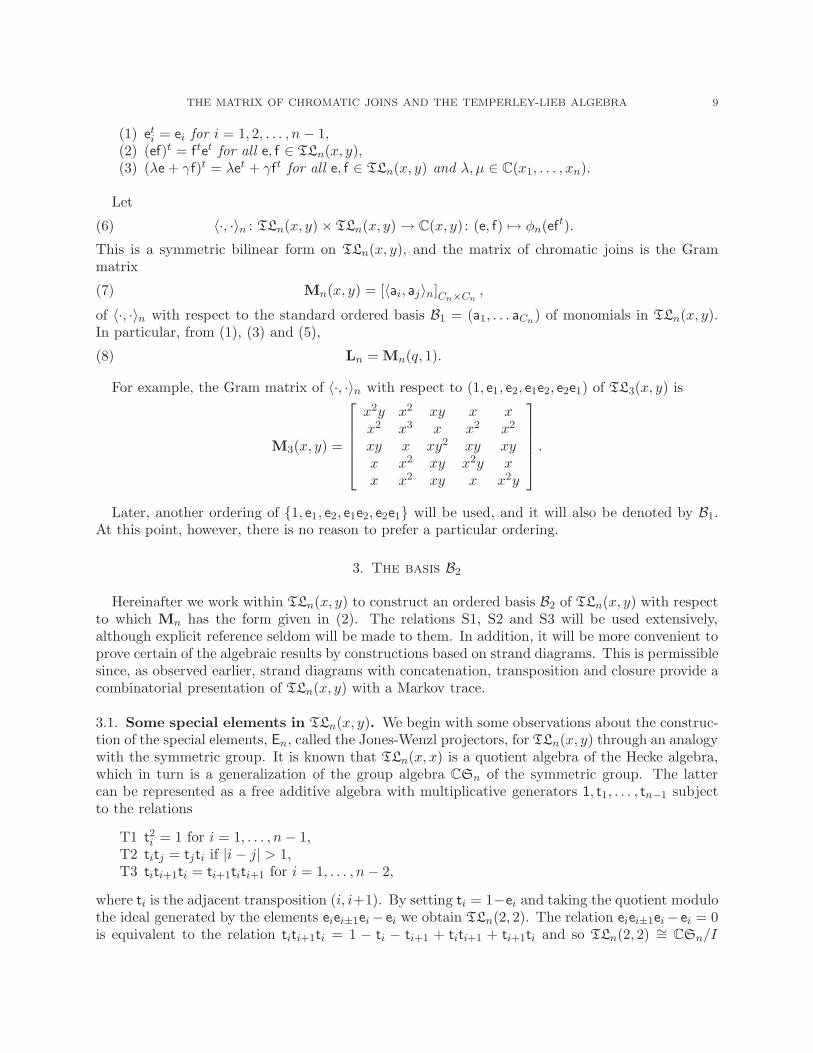


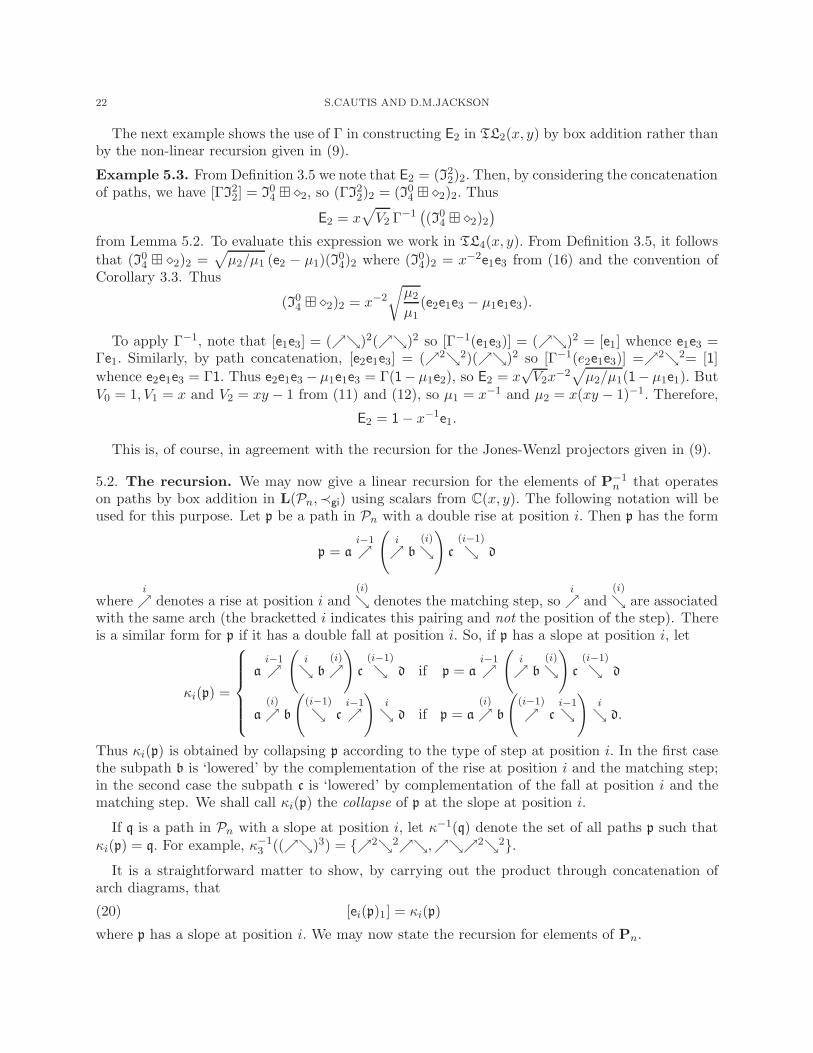


![FROM THE FRAMISATION OF THE TEMPERLEY{LIEB ALGEBRA …chlouveraki.perso.math.cnrs.fr/pdf/KinH.pdf · Jacon and Poulain d’Andecy in [JaPdA]. Using these stabilised traces and the](https://static.documents.pub/doc/80x56/5fbd67542dcad333e65448f9/from-the-framisation-of-the-temperleylieb-algebra-jacon-and-poulain-daandecy.jpg)


