The Measurement Calculus Vincent Danos Universit´ e Paris 7 & CNRS [email protected]Elham Kashefi IQC - University of Waterloo Christ Church - Oxford [email protected]Prakash Panangaden McGill University [email protected]September 25, 2006 Abstract Measurement-based quantum computation has emerged from the physics community as a new approach to quantum computation where the notion of measurement is the main driving force of computation. This is in contrast with the more traditional circuit model which is based on unitary operations. Among measurement-based quantum computation methods, the recently introduced one-way quantum computer [RB01] stands out as fundamental. We develop a rigorous mathematical model underlying the one-way quantum computer and present a concrete syntax and operational semantics for programs, which we call patterns, and an algebra of these patterns derived from a denotational semantics. More importantly, we present a calculus for reasoning locally and compositionally about these patterns. We present a rewrite theory and prove a general standardization theorem which allows all patterns to be put in a semantically equivalent standard form. Standardization has far-reaching consequences: a new physical architecture based on performing all the entanglement in the beginning, parallelization by exposing the dependency structure of measurements and expressiveness theorems. Furthermore we formalize several other measurement-based models e.g. Teleportation, Phase and Pauli models and present compositional embeddings of them into and from the one-way model. This allows us to transfer all the theory we develop for the one-way model to these mod- els. This shows that the framework we have developed has a general impact on measurement- based computation and is not just particular to the one-way quantum computer. 1 Introduction The emergence of quantum computation has changed our perspective on many fundamental aspects of computing: the nature of information and how it flows, new algorithmic design strategies and complexity classes and the very structure of computational models [NC00]. New challenges have been raised in the physical implementation of quantum computers. This paper is a contribution to a nascent discipline: quantum programming languages. This is more than a search for convenient notation, it is an investigation into the structure, scope and limits of quantum computation. The main issues are questions about how quantum processes are defined, how quantum algorithms compose, how quantum resources are used and how classical and quantum information interact. Quantum computation emerged in the early 1980s with Feynman’s observations about the dif- ficulty of simulating quantum systems on a classical computer. This hinted at the possibility of turning around the issue and exploiting the power of quantum systems to perform computational 1
Measurement-based quantum computation has emerged from the physics community as anew approach to quantum computation where the notion of measurement is the main drivingforce of computation. This is in contrast with the more traditional circuit model which is basedon unitary operations. Among measurement-based quantum computation methods, the recentlyintroduced one-way quantum computer [RB01] stands out as fundamental.
We develop a rigorous mathematical model underlying the one-way quantum computer andpresent a concrete syntax and operational semantics for programs, which we call patterns, and analgebra of these patterns derived from a denotational semantics. More importantly, we presenta calculus for reasoning locally and compositionally about these patterns. We present a rewritetheory and prove a general standardization theorem which allows all patterns to be put in asemantically equivalent standard form. Standardization has far-reaching consequences: a newphysical architecture based on performing all the entanglement in the beginning, parallelizationby exposing the dependency structure of measurements and expressiveness theorems.
Furthermore we formalize several other measurement-based models e.g.Teleportation, Phaseand Pauli models and present compositional embeddings of them into and from the one-waymodel. This allows us to transfer all the theory we develop for the one-way model to these mod-els. This shows that the framework we have developed has a general impact on measurement-based computation and is not just particular to the one-way quantum computer.
1 Introduction
The emergence of quantum computation has changed our perspective on many fundamental aspectsof computing: the nature of information and how it flows, new algorithmic design strategies andcomplexity classes and the very structure of computational models [NC00]. New challenges havebeen raised in the physical implementation of quantum computers. This paper is a contribution toa nascent discipline: quantum programming languages.
This is more than a search for convenient notation, it is an investigation into the structure,scope and limits of quantum computation. The main issues are questions about how quantumprocesses are defined, how quantum algorithms compose, how quantum resources are used and howclassical and quantum information interact.
Quantum computation emerged in the early 1980s with Feynman’s observations about the dif-ficulty of simulating quantum systems on a classical computer. This hinted at the possibility ofturning around the issue and exploiting the power of quantum systems to perform computational
1
tasks more efficiently than was classically possible. In the mid 1980s Deutsch [Deu87] and laterDeutsch and Jozsa [DJ92] showed how to use superposition – the ability to produce linear combi-nations of quantum states – to obtain computational speedup. This led to interest in algorithmdesign and the complexity aspects of quantum computation by computer scientists. The mostdramatic results were Shor’s celebrated polytime factorization algorithm [Sho94] and Grover’s sub-linear search algorithm [Gro98]. Remarkably one of the problematic aspects of quantum theory,the presence of non-local correlation – an example of which is called “entanglement” – turned outto be crucial for these algorithmic developments.
If efficient factorization is indeed possible in practice, then much of cryptography becomesinsecure as it is based on the difficulty of factorization. However, entanglement makes it possibleto design unconditionally secure key distribution [BB84, Eke91]. Furthermore, entanglement ledto the remarkable – but simple – protocol for transferring quantum states using only classicalcommunication [BBC+93]; this is the famous so-called “teleportation” protocol. There continues tobe tremendous activity in quantum cryptography, algorithmic design, complexity and informationtheory. Parallel to all this work there has been intense interest from the physics community toexplore possible implementations, see, for example, [NC00] for a textbook account of some of theseideas.
On the other hand, only recently has there been significant interest in quantum programminglanguages; i.e. the development of formal syntax and semantics and the use of standard machineryfor reasoning about quantum information processing. The first quantum programming languageswere variations on imperative probabilistic languages and emphasized logic and program develop-ment based on weakest preconditions [SZ00, O01]. The first definitive treatment of a quantumprogramming language was the flowchart language of Selinger [Sel04b]. It was based on combiningclassical control, as traditionally seen in flowcharts, with quantum data. It also gave a denotationalsemantics based on completely positive linear maps. The notion of quantum weakest preconditionswas developed in [DP04]. Later people proposed languages based on quantum control [AG05]. Thesearch for a sensible notion of higher-type computation [SV05, vT04] continues, but is problem-atic [Sel04c].
A related recent development is the work of Abramsky and Coecke [AC04, Coe04] where theydevelop a categorical axiomatization of quantum mechanics. This can be used to verify the correct-ness of quantum communication protocols. It is very interesting from a foundational point of viewand allows one to explore exactly what mathematical ingredients are required to carry out certainquantum protocols. This has also led to work on a categorical quantum logic [AD04].
The study of quantum communication protocols has led to formalizations based on processalgebras [GN05, JL04] and to proposals to use model checking for verifying quantum protocols. Asurvey and a complete list of references on this subject up to 2005 is available [Gay05].
These ideas have proven to be of great utility in the world of classical computation. The use oflogics, type systems, operational semantics, denotational semantics and semantic-based inferencemechanisms have led to notable advances such as: the use of model checking for verification,reasoning compositionally about security protocols, refinement-based programming methodologyand flow analysis.
The present paper applies this paradigm to a very recent development: measurement-basedquantum computation. None of the cited research on quantum programming languages is aimedat measurement-based computation. On the other hand, the work in the physics literature doesnot clearly separate the conceptual layers of the subject from implementation issues. A formal
2
treatment is necessary to analyze the foundations of measurement-based computation.So far the main framework to explore quantum computation has been the circuit model [Deu89],
based on unitary evolution. This is very useful for algorithmic development and complexity analysis[BV97]. There are other models such as quantum Turing machines [Deu85] and quantum cellularautomata [Wat95, vD96, DS96, SW04]. Although they are all proved to be equivalent from thepoint of view of expressive power, there is no agreement on what is the canonical model for exposingthe key aspects of quantum computation.
Recently physicists have introduced novel ideas based on the use of measurement and entangle-ment to perform computation [GC99, RB01, RBB03, Nie03]. This is very different from the circuitmodel where measurement is done only at the end to extract classical output. In measurement-basedcomputation the main operation to manipulate information and control computation is measure-ment. This is surprising because measurement creates indeterminacy, yet it is used to expressdeterministic computation defined by a unitary evolution.
The idea of computing based on measurements emerged from the teleportation protocol [BBC+93].The goal of this protocol is for an agent to transmit an unknown qubit to a remote agent withoutactually sending the qubit. This protocol works by having the two parties share a maximally en-tangled state called a Bell pair. The parties perform local operations – measurements and unitaries– and communicate only classical bits. Remarkably, from this classical information the secondparty can reconstruct the unknown quantum state. In fact one can actually use this to com-pute via teleportation by choosing an appropriate measurement [GC99]. This is the key idea ofmeasurement-based computation.
It turns out that the above method of computing is actually universal. This was first shownby Gottesman and Chuang [GC99] who used two-qubit measurements and given Bell pairs. LaterNielsen [Nie03] showed that one could do this with only 4-qubit measurements with no prior Bellpairs, however this works only probabilistically. Leung [Leu04] improved this to two qubits, but hermethod also works only probabilistically. Later Perdrix and Jorrand [Per03, PJ04] gave the minimalset measurements to perform universal quantum computing – but still in the probabilistic setting– and introduced the state-transfer and measurement-based quantum Turing machine. Finallythe one-way computer was invented by Raussendorf and Briegel [RB01, RB02] which used onlysingle-qubit measurements with a particular multi-party entangled state, the cluster state.
More precisely, a computation consists of a phase in which a collection of qubits are set up in astandard entangled state. Then measurements are applied to individual qubits and the outcomes ofthe measurements may be used to determine further measurements. Finally – again depending onmeasurement outcomes – local unitary operators, called corrections, are applied to some qubits; thisallows the elimination of the indeterminacy introduced by measurements. The phrase “one-way”is used to emphasize that the computation is driven by irreversible measurements.
There are at least two reasons to take measurement-based models seriously: one conceptualand one pragmatic. The main pragmatic reason is that the one-way model is believed by physiciststo lend itself to easier implementations [Nie04, CAJ05, BR05, TPKV04, TPKV06, WkJRR+05,KPA06, BES05, CCWD06, BBFM06]. Physicists have investigated various properties of the clusterstate and have accrued evidence that the physical implementation is scalable and robust againstdecoherence [Sch03, HEB04, DAB03, dNDM04b, dNDM04a, MP04, GHW05, HDB05, DHN06].Conceptually the measurement-based model highlights the role of entanglement and separates thequantum and classical aspects of computation; thus it clarifies, in particular, the interplay betweenclassical control and the quantum evolution process.
3
Our approach to understanding the structural features of measurement-based computation is todevelop a formal calculus. One can think of this as an “assembly language” for measurement-basedcomputation. Ours is the first programming framework specifically based on the one-way model. Wefirst develop a notation for such classically correlated sequences of entanglements, measurements,and local corrections. Computations are organized in patterns1, and we give a careful treatmentof the composition and tensor product (parallel composition) of patterns. We show next that suchpattern combinations reflect the corresponding combinations of unitary operators. An easy proofof universality follows.
So far, this is primarily a clarification of what was already known from the series of papersintroducing and investigating the properties of the one-way model [RB01, RB02, RBB03]. However,we work here with an extended notion of pattern, where inputs and outputs may overlap in anyway one wants them to, and this results in more efficient – in the sense of using fewer qubits –implementations of unitaries. Specifically, our universal set consists of patterns using only 2 qubits.From it we obtain a 3 qubit realization of the Rz rotations and a 14 qubit realization for thecontrolled-U family: a significant reduction over the hitherto known implementations.
The main point of this paper is to introduce a calculus of local equations over patterns thatexploits some special algebraic properties of the entanglement, measurement and correction op-erators. More precisely, we use the fact that that 1-qubit XY measurements are closed underconjugation by Pauli operators and the entanglement command belongs to the normalizer of thePauli group; these terms are explained in the appendix. We show that this calculus is sound in thatit preserves the interpretation of patterns. Most importantly, we derive from it a simple algorithmby which any general pattern can be put into a standard form where entanglement is done first,then measurements, then corrections. We call this standardization.
The consequences of the existence of such a procedure are far-reaching. Since entangling comesfirst, one can prepare the entire entangled state needed during the computation right at the start:one never has to do “on the fly” entanglements. Furthermore, the rewriting of a pattern to stan-dard form reveals parallelism in the pattern computation. In a general pattern, one is forced tocompute sequentially and to strictly obey the command sequence, whereas, after standardization,the dependency structure is relaxed, resulting in lower computational depth complexity. Last, theexistence of a standard form for any pattern also has interesting corollaries beyond implementationand complexity matters, as it follows from it that patterns using no dependencies, or using only therestricted class of Pauli measurements, can only realize a unitary belonging to the Clifford group,and hence can be efficiently simulated by a classical computer [Got97].
As we have noted before, there are other methods for measurement-based quantum comput-ing: the teleportation technique based on two-qubit measurements and the state-transfer approachbased on single qubit measurements and incomplete two-qubit measurements. We will analyze theteleportation model and its relation to the one-way model. We will show how our calculus can besmoothly extended to cover this case as well as new models that we introduce in this paper. Weget several benefits from our treatment. We get a workable syntax for handling the dependencies ofoperators on previous measurement outcomes just by mimicking the one obtained in the one-waymodel. This has never been done before for the teleportation model. Furthermore, we can use thisembedding to obtain a standardization procedure for the models. Finally these extended calculican be compositionally embedded back in the original one-way model. This clarifies the relation
1We use the word “pattern” rather than “program”, because this corresponds to the commonly used terminologyin the physics literature.
4
between different measurement-based models and shows that the one-way model of Raussendorfand Briegel is the canonical one.
This paper develops the one-way model ab initio but certain concepts that the reader may beunfamiliar with: qubits, unitaries, measurements, Pauli operators and the Clifford group are inan appendix. These are also readily accessible through the very thorough book of Nielsen andChuang [NC00].
In the next section we define the basic model, followed by its operational and denotationalsemantics, for completeness a simple proof of universality is given in section 4, this has appearedearlier in the physics literature [DKP05], in section 5 we develop the rewrite theory and prove thefundamental standardization theorem. In section 6 we develop several examples that illustrate theuse of our calculus in designing efficient patterns. In section 7 we prove some theorems about theexpressive power of the calculus in the absence of adaptive measurements. In section 8 we discussother measurement-based models and their compositional embedding to and from the one-waymodel. In section 9 we discuss further directions and some more related work. In the appendix wereview basic notions of quantum mechanics and quantum computation.
2 Measurement Patterns
We first develop a notation for 1-qubit measurement based computations. The basic commandsone can use in a pattern are:
• 1-qubit auxiliary preparation Ni
• 2-qubit entanglement operators Eij
• 1-qubit measurements Mαi
• and 1-qubit Pauli operators corrections Xi and Zi
The indices i, j represent the qubits on which each of these operations apply, and α is aparameter in [0, 2π]. Expressions involving angles are always evaluated modulo 2π. These types ofcommand will be referred to as N , E, M and C. Sequences of such commands, together with twodistinguished – possibly overlapping – sets of qubits corresponding to inputs and outputs, will becalled measurement patterns, or simply patterns. These patterns can be combined by compositionand tensor product.
Importantly, corrections and measurements are allowed to depend on previous measurementoutcomes. We shall prove later that patterns without these classical dependencies can only realizeunitaries that are in the Clifford group. Thus, dependencies are crucial if one wants to define auniversal computing model; that is to say, a model where all unitaries over ⊗nC2 can be realized.It is also crucial to develop a notation that will handle these dependencies. This is what we donow.
2.1 Commands
Preparation Ni prepares qubit i in state |+〉i. The entanglement commands are defined as Eij :=∧Zij (controlled-Z), while the correction commands are the Pauli operators Xi and Zi.
5
Measurement Mαi is defined by orthogonal projections on
|+α〉 := 1√2(|0〉+ eiα|1〉)
|−α〉 := 1√2(|0〉 − eiα|1〉)
followed by a trace-out operator. The parameter α ∈ [0, 2π] is called the angle of the measurement.For α = 0, α = π
2 , one obtains the X and Y Pauli measurements. Operationally, measurements willbe understood as destructive measurements, consuming their qubit. The outcome of a measurementdone at qubit i will be denoted by si ∈ Z2. Since one only deals here with patterns where qubitsare measured at most once (see condition (D1) below), this is unambiguous. We take the specificconvention that si = 0 if under the corresponding measurement the state collapses to |+α〉, andsi = 1 if to |−α〉.
Outcomes can be summed together resulting in expressions of the form s =∑
i∈I si which wecall signals, and where the summation is understood as being done in Z2. We define the domainof a signal as the set of qubits on which it depends.
As we have said before, both corrections and measurements may depend on signals. Depen-dent corrections will be written Xs
i and Zsi and dependent measurements will be written t[Mαi ]s,
where s, t ∈ Z2 and α ∈ [0, 2π]. The meaning of dependencies for corrections is straightforward:X0i = Z0
i = I, no correction is applied, while X1i = Xi and Z1
i = Zi. In the case of dependentmeasurements, the measurement angle will depend on s, t and α as follows:
t[Mαi ]s := M
(−1)sα+tπi (1)
so that, depending on the parities of s and t, one may have to modify the α to one of −α, α + πand −α+ π. These modifications correspond to conjugations of measurements under X and Z:
XiMαi Xi = M−α
i (2)ZiM
αi Zi = Mα+π
i (3)
accordingly, we will refer to them as the X and Z-actions. Note that these two actions commute,since −α+ π = −α− π up to 2π, and hence the order in which one applies them does not matter.
As we will see later, relations (2) and (3) are key to the propagation of dependent corrections,and to obtaining patterns in the standard entanglement, measurement and correction form. Sincethe measurements considered here are destructive, the above equations actually simplify to
Mαi Xi = M−α
i (4)Mαi Zi = Mα−π
i (5)
Another point worth noticing is that the domain of the signals of a dependent command, be it ameasurement or a correction, represents the set of measurements which one has to do before onecan determine the actual value of the command.
We have completed our catalog of basic commands, including dependent ones, and we turnnow to the definition of measurement patterns. For convenient reference, the language syntax issummarized in Figure 1.
6
S := 0, 1, si, S + S SignalsA := Ni Preparations
Eij Entanglementst[Mα
i ]s MeasurementsXsi , Z
si Corrections
Figure 1: 1-qubit based measurement language syntax
2.2 Patterns
Definition 1 Patterns consists of three finite sets V , I, O, together with two injective maps ι :I → V and o : O → V and a finite sequence of commands An . . . A1, read from right to left, applyingto qubits in V in that order, i.e. A1 first and An last, such that:
(D0) no command depends on an outcome not yet measured;
(D1) no command acts on a qubit already measured;
(D2) no command acts on a qubit not yet prepared, unless it is an input qubit;
(D3) a qubit i is measured if and only if i is not an output.
The set V is called the pattern computation space, and we write HV for the associated quantumstate space ⊗i∈V C2. To ease notation, we will omit the maps ι and o, and write simply I, O insteadof ι(I) and o(O). Note, however, that these maps are useful to define classical manipulations ofthe quantum states, such as permutations of the qubits. The sets I, O are called respectively thepattern inputs and outputs, and we write HI , and HO for the associated quantum state spaces. Thesequence An . . . A1 is called the pattern command sequence, while the triple (V, I,O) is called thepattern type.
To run a pattern, one prepares the input qubits in some input state ψ ∈ HI , while the non-inputqubits are all set to the |+〉 state, then the commands are executed in sequence, and finally the resultof the pattern computation is read back from outputs as some φ ∈ HO. Clearly, for this procedureto succeed, we had to impose the (D0), (D1), (D2) and (D3) conditions. Indeed if (D0) fails, thenat some point of the computation, one will want to execute a command which depends on outcomesthat are not known yet. Likewise, if (D1) fails, one will try to apply a command on a qubit thathas been consumed by a measurement (recall that we use destructive measurements). Similarly, if(D2) fails, one will try to apply a command on a non-existent qubit. Condition (D3) is there tomake sure that the final state belongs to the output space HO, i.e., that all non-output qubits, andonly non-output qubits, will have been consumed by a measurement when the computation ends.
We write (D) for the conjunction of our definiteness conditions (D0), (D1), (D2) and (D3).Whether a given pattern satisfies (D) or not is statically verifiable on the pattern command se-quence. We could have imposed a simple type system to enforce these constraints but, in theinterests of notational simplicity, we chose not to do so.
Here is a concrete example:
H := ({1, 2}, {1}, {2}, Xs12 M
01E12N2)
7
with computation space {1, 2}, inputs {1}, and outputs {2}. To run H, one first prepares the firstqubit in some input state ψ, and the second qubit in state |+〉, then these are entangled to obtain∧Z12(ψ1 ⊗ |+〉2). Once this is done, the first qubit is measured in the |+〉, |−〉 basis. Finally an Xcorrection is applied on the output qubit, if the measurement outcome was s1 = 1. We will do thiscalculation in detail later, and prove that this pattern implements the Hadamard operator H.
In general, a given pattern may use auxiliary qubits that are neither input nor output qubits.Usually one tries to use as few such qubits as possible, since these contribute to the space complexityof the computation.
A last thing to note is that one does not require inputs and outputs to be disjoint subsets ofV . This, seemingly innocuous, additional flexibility is actually quite useful to give parsimoniousimplementations of unitaries [DKP05]. While the restriction to disjoint inputs and outputs isunnecessary, it has been discussed whether imposing it results in patterns that are easier to realizephysically. Recent work [HEB04, BR05, CAJ05] however, seems to indicate it is not the case.
2.3 Pattern combination
We are interested in how one can combine patterns in order to obtain bigger ones.The first way to combine patterns is by composing them. Two patterns P1 and P2 may be
composed if V1 ∩ V2 = O1 = I2. Provided that P1 has as many outputs as P2 has inputs, byrenaming the pattern qubits, one can always make them composable.
Definition 2 The composite pattern P2P1 is defined as:— V := V1 ∪ V2, I = I1, O = O2,— commands are concatenated.
The other way of combining patterns is to tensor them. Two patterns P1 and P2 may be tensoredif V1 ∩ V2 = ∅. Again one can always meet this condition by renaming qubits in a way that thesesets are made disjoint.
Definition 3 The tensor pattern P1 ⊗ P2 is defined as:— V = V1 ∪ V2, I = I1 ∪ I2, and O = O1 ∪O2,— commands are concatenated.
In contrast to the composition case, all the unions involved here are disjoint. Therefore commandsfrom distinct patterns freely commute, since they apply to disjoint qubits, and when we say thatcommands have to be concatenated, this is only for definiteness. It is routine to verify that thedefiniteness conditions (D) are preserved under composition and tensor product.
Before turning to this matter, we need a clean definition of what it means for a pattern toimplement or to realize a unitary operator, together with a proof that the way one can combinepatterns is reflected in their interpretations. This is key to our proof of universality.
3 The semantics of patterns
In this section we give a formal operational semantics for the pattern language as a probabilisticlabeled transition system. We define deterministic patterns and thereafter concentrate on them.We show that deterministic patterns compose. We give a denotational semantics of deterministicpatterns; from the construction it will be clear that these two semantics are equivalent.
8
Besides quantum states, which are non-zero vectors in some Hilbert space HV , one needs aclassical state recording the outcomes of the successive measurements one does in a pattern. If welet V stand for the finite set of qubits that are still active (i.e. not yet measured) and W standsfor the set of qubits that have been measured (i.e. they are now just classical bits recording themeasurement outcomes), it is natural to define the computation state space as:
S := ΣV,WHV × ZW2 .
In other words the computation states form a V,W -indexed family of pairs2 q, Γ, where q is aquantum state from HV and Γ is a map from some W to the outcome space Z2. We call thisclassical component Γ an outcome map, and denote by ∅ the empty outcome map in Z∅
2 . We willtreat these states as pairs unless it becomes important to show how V and W are altered during acomputation, as happens during a measurement.
3.1 Operational semantics
We need some preliminary notation. For any signal s and classical state Γ ∈ ZW2 , such that thedomain of s is included in W , we take sΓ to be the value of s given by the outcome map Γ. That isto say, if s =
∑I si, then sΓ :=
∑I Γ(i) where the sum is taken in Z2. Also if Γ ∈ ZW2 , and x ∈ Z2,
we define:Γ[x/i](i) = x, Γ[x/i](j) = Γ(j) for j 6= i
which is a map in ZW∪{i}2 .
We may now view each of our commands as acting on the state space S, we have suppressed Vand W in the first 4 commands:
q,Γ Ni−→ q ⊗ |+〉i,Γq,Γ
Eij−→ ∧Zijq,Γq,Γ
Xsi−→ XsΓ
i q,Γ
q,ΓZs
i−→ ZsΓi q,Γ
V ∪ {i},W, q,Γt[Mα
i ]s
−→ V,W ∪ {i}, 〈+αΓ |iq,Γ[0/i]
V ∪ {i},W, q,Γt[Mα
i ]s
−→ V,W ∪ {i}, 〈−αΓ |iq,Γ[1/i]
where αΓ = (−1)sΓα + tΓπ following equation (1). Note how the measurement moves an indexfrom V to W ; a qubit once measured cannot be neasured again. Suppose q ∈ HV , for the aboverelations to be defined, one needs the indices i, j on which the various command apply to be in V .One also needs Γ to contain the domains of s and t, so that sΓ and tΓ are well-defined. This willalways be the case during the run of a pattern because of condition (D).
All commands except measurements are deterministic and only modify the quantum part ofthe state. The measurement actions on S are not deterministic, so that these are actually binaryrelations on S, and modify both the quantum and classical parts of the state. The usual conventionhas it that when one does a measurement the resulting state is renormalized and the probabilitiesare associated with the transition. We do not adhere to this convention here, instead we leave thestates unnormalized. The reason for this choice of convention is that this way, the probability of
2These are actually quadruples of the form (V, W, q, Γ), unless necessary we will suppress the V and the W .
9
reaching a given state can be read off its norm, and the overall treatment is simpler. As we willshow later, all the patterns implementing unitary operators will have the same probability for allthe branches and hence we will not need to carry these probabilities explicitly.
We introduce an additional command called signal shifting :
q,ΓSs
i−→ q,Γ[Γ(i) + sΓ/i]
It consists in shifting the measurement outcome at i by the amount sΓ. Note that the Z-action leavesmeasurements globally invariant, in the sense that |+α+π〉, |−α+π〉 = |−α〉, |+α〉. Thus changing αto α+ π amounts to swapping the outcomes of the measurements, and one has:
t[Mαi ]s = Sti
0[Mαi ]s (6)
and signal shifting allows to dispose of the Z action of a measurement, resulting sometimes inconvenient optimizations of standard forms.
3.2 Denotational semantics
Let P be a pattern with computation space V , inputs I, outputs O and command sequenceAn . . . A1. To execute a pattern, one starts with some input state q in HI , together with theempty outcome map ∅. The input state q is then tensored with as many |+〉s as there are non-inputs in V (the N commands), so as to obtain a state in the full space HV . Then E, M andC commands in P are applied in sequence from right to left. We can summarize the situation asfollows:
HI
��
// HO
HI × Z∅2
prep // HV × Z∅2
A1...An // HO × ZVrO2
OO
If m is the number of measurements, which is also the number of non outputs, then the run mayfollow 2m different branches. Each branch is associated with a unique binary string s of length m,representing the classical outcomes of the measurements along that branch, and a unique branchmap As representing the linear transformation from HI to HO along that branch. This map isobtained from the operational semantics via the sequence (qi,Γi) with 1 ≤ i ≤ n+ 1, such that:
q1,Γ1 = q ⊗ |+ . . .+〉,∅qn+1 = q′ 6= 0
and for all i ≤ n : qi,ΓiAi−→ qi+1,Γi+1.
Definition 4 A pattern P realizes a map on density matrices ρ given by ρ 7→∑
sA†s(ρ)As. We
write [[P]] for the map realized by P.
Proposition 5 Each pattern realizes a completely positive trace preserving map.
Proof. Later on we will show that every pattern can be put in a semantically equivalent formwhere all the preparations and entanglements appear first, followed by a sequence of measurementsand finally local Pauli corrections. Hence branch maps decompose as As = CsΠsU , where Cs is a
10
unitary map over HO collecting all corrections on outputs, Πs is a projection from HV to HO rep-resenting the particular measurements performed along the branch, and U is a unitary embeddingfrom HI to HV collecting the branch preparations, and entanglements. Note that U is the same onall branches. Therefore, ∑
sA†sAs =
∑s U
†Π†sC
†sCsΠsU
=∑
s U†Π†
sΠsU= U †(
∑s Πs)U
= U †U = I
where we have used the fact that Cs is unitary, Πs is a projection and U is independent ofthe branches and is also unitary. Therefore the map T (ρ) :=
∑sAs(ρ)A
†s is a trace-preserving
completely-positive map (cptp-map), explicitly given as a Kraus decomposition. 2
Hence the denotational semantics of a pattern is a cptp-map. In our denotational semantics weview the pattern as defining a map from the input qubits to the output qubits. We do not explicitlyrepresent the result of measuring the final qubits; these may be of interest in some cases. Techniquesfor dealing with classical output explicitly are given by Selinger [Sel04b] and Unruh [Unr05].
Definition 6 A pattern is said to be deterministic if it realizes a cptp-map that sends pure statesto pure states. A pattern is said to be strongly deterministic when branch maps are equal.
This is equivalent to saying that for a deterministic pattern branch maps are proportional, thatis to say, for all q ∈ HI and all s1, s2 ∈ Zn2 , As1(q) and As2(q) differ only up to a scalar. For astrongly deterministic pattern we have for all s1, s2 ∈ Zn2 , As1 = As2 .
Proposition 7 If a pattern is strongly deterministic, then it realizes a unitary embedding.
Proof. Define T to be the map realized by the pattern. We have T =∑
sA†sAs. Since the pattern
in strongly deterministic all the branch maps are the same. Define A to be 2n/2As, then A mustbe a unitary embedding, because A†A = I. 2
3.3 Short examples
For the rest of paper we assume that all the non-input qubits are prepared in the state |+〉 andhence for simplicity we omit the preparation commands NIc .
First we give a quick example of a deterministic pattern that has branches with different proba-bilities. Its type is V = {1, 2}, I = O = {1}, and its command sequence is Mα
2 . Therefore, startingwith input q, one gets two branches:
q ⊗ |+〉,∅Mα
2−→
12(1 + e−iα)q,∅[0/2]
12(1− e−iα)q,∅[1/2]
Thus this pattern is indeed deterministic, and implements the identity up to a global phase, andyet the two branches have respective probabilities (1 + cosα)/2 and (1 − cosα)/2, which are notequal in general and hence this pattern is not strongly deterministic.
There is an interesting variation on this first example. The pattern of interest, call it T , hasthe same type as above with command sequence Xs2
1 M02E12. Again, T is deterministic, but not
11
strongly deterministic: the branches have different probabilities, as in the preceding example. Now,however, these probabilities may depend on the input. The associated transformation is a cptp-map,T (ρ) := AρA† +BρB† with:
A :=(
1 00 0
), B :=
(0 10 0
)One has A†A+B†B = I, so T is indeed a completely positive and trace-preserving linear map andT (|ψ〉〈ψ|) = 〈ψ,ψ〉|0〉〈0| and clearly for no unitary U does one have T (ρ) := UρU †.
For our final example, we return to the pattern H, already defined above. Consider the patternwith the same qubit space {1, 2}, and the same inputs and outputs I = {1}, O = {2}, as H, butwith a shorter command sequence namely M0
1E12. Starting with input q = (a|0〉 + b|1〉)|+〉, onehas two computation branches, branching at M0
and since ‖a+ b‖2 + ‖a− b‖2 = 2(‖a‖2 + ‖b‖2), both transitions happen with equal probabilities 12 .
Both branches end up with non proportional outputs, so the pattern is not deterministic. However,if one applies the local correction X2 on either of the branches’ ends, both outputs will be made tocoincide. If we choose to let the correction apply to the second branch, we obtain the pattern H,already defined. We have just proved H = UH, that is to say H realizes the Hadamard operator.
3.4 Compositionality of the Denotational Semantics
With our definitions in place, we will show that the denotational semantics is compositional.
Theorem 1 For two patterns P1 and P2 we have [[P1P2]] = [[P2]][[P1]] and [[P1⊗P2]] = [[P2]]⊗ [[P1]].
Proof. Recall that two patterns P1, P2 may be combined by composition provided P1 has as manyoutputs as P2 has inputs. Suppose this is the case, and suppose further that P1 and P2 respectivelyrealize some cptp-maps T1 and T2. We need to show that the composite pattern P2P1 realizes T2T1.
Indeed, the two diagrams representing branches in P1 and P2:
HI1
��
// HO1 HI2
��
// HO2
HI1 × Z∅2
p1// HV1 × Z∅2
// HO1 × ZV1rO12
OO
HI2 × Z∅2
p2// HV2 × Z∅2
// HO2 × ZV2rO22
OO
can be pasted together, since O1 = I2, and HO1 = HI2 . But then, it is enough to notice 1) thatpreparation steps p2 in P2 commute with all actions in P1 since they apply on disjoint sets of qubits,and 2) that no action taken in P2 depends on the measurements outcomes in P1. It follows thatthe pasted diagram describes the same branches as does the one associated to the composite P2P1.
A similar argument applies to the case of a tensor combination, and one has that P2 ⊗ P1
realizes T2 ⊗ T1. 2
12
If one wanted to give a categorical treatment3 one can define a category where the objects arefinite sets representing the input and output qubits and the morphisms are the patterns. This isclearly a monoidal category with our tensor operation as the monoidal structure. One can show thatthe denotational semantics gives a monoidal functor into the category of superoperators or into anysuitably enriched strongly compact closed category [AC04] or dagger category [Sel05a]. It would bevery interesting to explore exactly what additional categorical structures are required to interpretthe measurement calculus presented below. Duncan Ross[Dun05] has skectched a polycategoricalpresentation of our measurement calculus.
4 Universality
Define the two following patterns on V = {1, 2}:
J (α) := Xs12 M
−α1 E12 (7)
∧Z := E12 (8)
with I = {1}, O = {2} in the first pattern, and I = O = {1, 2} in the second. Note that the secondpattern does have overlapping inputs and outputs.
Proposition 8 The patterns J (α) and ∧Z are universal.
Proof. First, we claim J (α) and ∧Z respectively realize J(α) and ∧Z, with:
J(α) := 1√2
(1 eiα
1 −eiα)
We have already seen in our example that J (0) = H implements H = J(0), thus we already knowthis in the particular case where α = 0. The general case follows by the same kind of computation.4
The case of ∧Z is obvious.Second, we know that these unitaries form a universal set for ⊗nC2 [DKP05]. Therefore, fromthe preceding section, we infer that combining the corresponding patterns will generate patternsrealizing any unitary in ⊗nC2. 2
These patterns are indeed among the simplest possible. As a consequence, in the section devotedto examples, we will find that our implementations often have lower space complexity than thetraditional implementations.
Remarkably, in our set of generators, one finds a single measurement and a single dependency,which occurs in the correction phase of J (α). Clearly one needs at least one measurement, sincepatterns without measurements can only implement unitaries in the Clifford group. It is also truethat dependencies are needed for universality, but we have to wait for the development of themeasurement calculus in the next section to give a proof of this fact.
3The rest of the paragraph can be omitted without loss of continuity.
4Equivalently, this follows from J(α) = HP (α), with P (α) =
„1 00 eiα
«and:
Xs12 M−α
1 E12 = Xs12 M0
1 P (α)1E12 = HP (α)1.
13
5 The measurement calculus
We turn to the next important matter of the paper, namely standardization. The idea is quitesimple. It is enough to provide local pattern rewrite rules pushing Es to the beginning of thepattern, and Cs to the end.
5.1 The equations
The expressions appearing as commands are all linear operators on Hilbert space. The equality thatwe consider is equality as operators. Thus our equations are justified by the algebra of operators.This equality implies equality in the denotational semantics.
A first set of equations give means to propagate local Pauli corrections through the entanglingoperator Eij . Because Eij = Eji, there are only two cases to consider:
EijXsi = Xs
i ZsjEij (9)
EijZsi = ZsiEij (10)
These equations are easy to verify and are natural since Eij belongs to the Clifford group, andtherefore maps under conjugation the Pauli group to itself.
A second set of equations give means to push corrections through measurements acting on thesame qubit. Again there are two cases:
t[Mαi ]sXr
i = t[Mαi ]s+r (11)
t[Mαi ]sZri = t+r[Mα
i ]s (12)
These equations follow easily from equations (4) and (5). They express the fact that the measure-ments Mα
i are closed under conjugation by the Pauli group, very much like equations (9) and (10)express the fact that the Pauli group is closed under conjugation by the entanglements Eij .
Define the following convenient abbreviations:
[Mαi ]s := 0[Mα
i ]s, t[Mαi ] := t[Mα
i ]0, Mαi := 0[Mα
i ]0,
Mxi := M0
i , Myi := M
π2i
Particular cases of the equations above are:
Mxi X
si = Mx
i
Myi X
si = [My
i ]s = s[Myi ] = My
i Zsi
The first equation, follows from the fact that −0 = 0, so the X action on Mxi is trivial; the second
equation, is because −π2 is equal π2 + π modulo 2π, and therefore the X and Z actions coincide on
Myi . So we obtain the following:
t[Mxi ]s = t[Mx
i ] (13)t[My
i ]s = s+t[Myi ] (14)
which we will use later to prove that patterns with measurements of the form Mx and My mayonly realize unitaries in the Clifford group.
14
5.2 The rewrite rules
We now define a set of rewrite rules, obtained by orienting the equations above5:
EijXsi ⇒ Xs
i ZsjEij EX
EijZsi ⇒ ZsiEij EZ
t[Mαi ]sXr
i ⇒ t[Mαi ]s+r MX
t[Mαi ]sZri ⇒ r+t[Mα
i ]s MZ
to which we need to add the free commutation rules, obtained when commands operate on disjointsets of qubits:
EijA~k ⇒ A~kEij where A is not an entanglementA~kX
si ⇒ Xs
iA~k where A is not a correctionA~kZ
si ⇒ ZsiA~k where A is not a correction
where ~k represent the qubits acted upon by command A, and are supposed to be distinct from iand j. Clearly these rules could be reversed since they hold as equations but we are orienting themthis way in order to obtain termination.
Condition (D) is easily seen to be preserved under rewriting.Under rewriting, the computation space, inputs and outputs remain the same, and so do the
entanglement commands. Measurements might be modified, but there is still the same numberof them, and they still act on the same qubits. The only induced modifications concern localcorrections and dependencies. If there was no dependency at the start, none will be created in therewriting process.
In order to obtain rewrite rules, it was essential that the entangling command (∧Z) belongsto the normalizer of the Pauli group. The point is that the Pauli operators are the correctionoperators and they can be dependent, thus we can commute the entangling commands to thebeginning without inheriting any dependency. Therefore the entanglement resource can indeed beprepared at the outset of the computation.
5.3 Standardization
Write P ⇒ P ′, respectively P ⇒? P ′, if both patterns have the same type, and one obtains thecommand sequence of P ′ from the command sequence of P by applying one, respectively anynumber, of the rewrite rules of the previous section. We say that P is standard if for no P ′, P ⇒ P ′
and the procedure of writing a pattern to standard form is called standardization6.One of the most important results about the rewrite system is that it has the desirable properties
of determinacy (confluence) and termination (standardization). In other words, we will show thatfor all P, there exists a unique standard P ′, such that P ⇒? P ′. It is, of course, crucial that thestandardization process leaves the semantics of patterns invariant. This is the subject of the nextsimple, but important, proposition,
Proposition 9 Whenever P ⇒? P ′, [[P]] = [[P ′]].5Recall that patterns are executed from right to left.6We use the word “standardization” instead of the more usual “normalization” in order not to cause terminological
confusion with the physicists’ notion of normalization.
15
Proof. It is enough to prove it when P ⇒ P ′. The first group of rewrites has been proved to besound in the preceding subsections, while the free commutation rules are obviously sound. 2
We now begin the main proof of this section. First, we prove termination.
Theorem 2 (Termination) All rewriting sequences beginning with a pattern P terminate afterfinitely many steps; or, equivalently, for all P there exists finitely many P ′ such that P ⇒? P ′
where the P ′ are standard.
Proof. Suppose P has command sequence An . . . A1; so the number of commands is n. Lete ≤ n be the number of E commands in P. As we have noted earlier, this number is invariantunder ⇒. Moreover E commands in P can be ordered by increasing depth, read from right to left,and this order, written <E , is also invariant, since EE commutations are forbidden explicitly inthe free commutation rules.
Define the following depth function d on E and C commands in P:
d(Ai) ={i if Ai = Ejkn− i if Ai = Cj
Define further the following sequence of length e, dE(P)(i) is the depth of the E-command of ranki according to <E . By construction this sequence is strictly increasing. Finally, we define themeasure m(P) := (dE(P), dC(P)) with:
dC(P) =∑
C∈P d(C)
We claim the measure we just defined decreases lexicographically under rewriting, in other wordsP ⇒ P ′ implies m(P) > m(P ′), where < is the lexicographic ordering on Ne+1.
To clarify these definitions, consider the following example. Suppose P’s command sequence isof the form EXZE, then e = 2, dE(P) = (1, 4), and m(P) = (1, 4, 3). For the command sequenceEEX we get that e = 2, dE(P) = (2, 3) and m(P) = (2, 3, 2). Now, if one considers the rewriteEEX ⇒ EXZE, the measure of the left hand side is (2, 3, 2), while the measure of the right handside, as said, is (1, 4, 3), and indeed (2, 3, 2) > (1, 4, 3). Intuitively the reason is clear: the Cs arebeing pushed to the left, thus decreasing the depths of Es, and concomitantly, the value of dE .
Let us now consider all cases starting with an EC rewrite. Suppose the E command underrewrite has depth d and rank i in the order <E . Then all Es of smaller rank have same depth inthe right hand side, while E has now depth d − 1 and still rank i. So the right hand side has astrictly smaller measure. Note that when C = X, because of the creation of a Z (see the exampleabove), the last element of m(P) may increase, and for the same reason all elements of index j > iin dE(P) may increase. This is why we are working with a lexicographical ordering.
Suppose now one does an MC rewrite, then dC(P) strictly decreases, since one correction isabsorbed, while all E commands have equal or smaller depths. Again the measure strictly decreases.
Next, suppose one does an EA rewrite, and the E command under rewrite has depth d and ranki. Then it has depth d−1 in the right hand side, and all other E commands have invariant depths,since we forbade the case when A is itself an E. It follows that the measure strictly decreases.
Finally, upon an AC rewrite, all E commands have invariant depth, except possibly one whichhas smaller depth in the case A = E, and dC(P) decreases strictly because we forbade the casewhere A = C. Again the claim follows.
16
So all rewrites decrease our ordinal measure, and therefore all sequences of rewrites are finite,and since the system is finitely branching (there are no more than n possible single step rewriteson a given sequence of length n), we get the statement of the theorem. 2
The next theorem establishes the important determinacy property and furthermore shows thatthe standard patterns have a certain canonical form which we call the NEMC form. The precisedefinition is:
Definition 10 A pattern has a NEMC form if its commands occur in the order of Ns first, thenEs , then Ms, and finally Cs.
We will usually just say “EMC” form since we can assume that all the auxiliary qubits are preparedin the |+〉 state we usually just elide these N commands.
Theorem 3 (Confluence) For all P, there exists a unique standard P ′, such that P ⇒? P ′, andP ′ is in EMC form.
Proof. Since the rewriting system is terminating, confluence follows from local confluence 7 byNewman’s lemma, see, for example, [Bar84]. The uniqueness of the standard is form an immediateconsequence.
We look for critical pairs, that is occurrences of three successive commands where two rules canbe applied simultaneously. One finds that there are only five types of critical pairs, of these thethree involve the N command, these are of the form: NMC, NEC and NEM ; and the remainingtwo are: EijMkCk with i, j and k all distinct, EijMkCl with k and l distinct. In all cases localconfluence is easily verified.
Suppose now P ′ does not satisfy the EMC form conditions. Then, either there is a pattern EAwith A not of type E, or there is a pattern AC with A not of type C. In the former case, E andA must operate on overlapping qubits, else one may apply a free commutation rule, and A maynot be a C since in this case one may apply an EC rewrite. The only remaining case is when Ais of type M , overlapping E’s qubits, but this is what condition (D1) forbids, and since (D1) ispreserved under rewriting, this contradicts the assumption. The latter case is even simpler. 2
We have shown that under rewriting any pattern can be put in EMC form, which is what wewanted. We actually proved more, namely that the standard form obtained is unique. However,one has to be a bit careful about the significance of this additional piece of information. Note firstthat uniqueness is obtained because we dropped the CC and EE free commutations, thus having arigid notion of command sequence. One cannot put them back as rewrite rules, since they obviouslyruin termination and uniqueness of standard forms.
A reasonable thing to do, would be to take this set of equations as generating an equivalencerelation on command sequences, call it ≡, and hope to strengthen the results obtained so far, byproving that all reachable standard forms are equivalent.
But this is too naive a strategy, since E12X1X2 ≡ E12X2X1, and:
E12Xs1X
t2 ⇒? Xs
1Zs2X
t2Z
t1E12
≡ Xs1Z
t1Z
s2X
t2E12
7This means that whenever two rewrite rules can be applied to a term t yielding t1 and t2, one can rewrite botht1 and t2 to a common third term t3, possibly in many steps.
17
obtaining an expression which is not symmetric in 1 and 2. To conclude, one has to extend ≡to include the additional equivalence Xs
1Zt1 ≡ Zt1X
s1 , which fortunately is sound since these two
operators are equal up to a global phase. Thus, these are all equivalent in our semantics of patterns.We summarize this discussion as follows.
Definition 11 We define an equivalence relation ≡ on patterns by taking all the rewrite rules asequations and adding the equation Xs
1Zt1 ≡ Zt1X
s1 and generating the smallest equivalence relation.
With this definition we can state the following proposition.
Proposition 12 All patterns that are equivalent by ≡ are equal in the denotational semantics.
This≡ relation preserves both the type (the (V, I,O) triple) and the underlying entanglement graph.So clearly semantic equality does not entail equality up to ≡. In fact, by composing teleportationpatterns one obtains infinitely many patterns for the identity which are all different up to ≡. Onemay wonder whether two patterns with same semantics, type and underlying entanglement graphare necessarily equal up to ≡. This is not true either. One has J(α)J(0)J(β) = J(α + β) =J(β)J(0)J(α) (where J(α) is defined in Section 4), and this readily gives a counter-example.
We can now formally describe a simple standardization algorithm.
Algorithm 1 Input: A pattern P on |V | = N qubits with command sequence AM · · ·A1.Output: An equivalent pattern P ′ in NEMC form.
1. Commute all the preparation commands (new qubits) to the right side.
2. Commute all the correction commands to the left side using the EC and MC rewriting rules.
3. Commute all the entanglement commands to the right side after the preparation commands.
Note that since each qubit can be entangled with at most N − 1 other qubits, and can bemeasured or corrected only once, we have O(N2) entanglement commands and O(N) measurementcommands. According to the definiteness condition, no command acts on a qubit not yet prepared,hence the first step of the above algorithm is based on trivial commuting rules; the same is truefor the last step as no entanglement command can act on a qubit that has been measured. Bothsteps can be done in O(N2). The real complexity of the algorithm comes from the second stepand the EX commuting rule. In the worst case scenario, commuting an X correction to the leftmight create O(N2) other Z corrections, each of which has to be commuted to the left themselves.Thus one can have at most O(N3) new corrections, each of which has to be commuted past O(N2)measurement or entanglement commands. Therefore the second step, and hence the algorithm, hasa worst case complexity of O(N5); if we take the length of the pattern to be the parameter thenN is O(n2) so the running time is O(n
52 ) in terms of n.
We conclude this subsection by emphasizing the importance of the EMC form. Since theentanglement can always be done first, we can always derive the entanglement resource needed forthe whole computation right at the beginning. After that only local operations will be performed.This will separate the analysis of entanglement resource requirements from the classical control.Furthermore, this makes it possible to extract the maximal parallelism for the execution of thepattern since the necessary dependecies are explicitly expressed, see the example in section 6 forfurther discussion. Finally, the EMC form provides us with tools to prove general theorems aboutpatterns, such as the fact that they always compute cptp-maps and the expressiveness theorems ofsection 7.
18
5.4 Signal shifting
One can extend the calculus to include the signal shifting command Sti . This allows one to disposeof dependencies induced by the Z-action, and obtain sometimes standard patterns with smallercomputational depth complexity, as we will see in the next section which is devoted to examples.
t[Mαi ]s ⇒ Sti [M
αi ]s
XsjS
ti ⇒ StiX
s[t+si/si]j
ZsjSti ⇒ StiZ
s[t+si/si]j
t[Mαj ]sSri ⇒ Sri
t[r+si/si][Mαj ]s[r+si/si]
where s[t/si] denotes the substitution of si with t in s, s, t being signals. Note that when we writea t explicitly on the upper left of an M , we mean that t 6= 0. The first additional rewrite rule wasalready introduced as equation (6), while the other ones merely propagate the signal shift. Clearlyone can dispose of Sti when it hits the end of the pattern command sequence. We will refer to thisnew set of rules as ⇒S .
It is important to note that both theorem 2 and 3 still hold for this extended rewriting system.In order to prove termination one can start with the EMC form and then adapt the proof ofTheorem 2 by defining a depth function for a signal shift similar to the depth of a correctioncommand. As with the correction, signal shifts can also be commuted to the left hand side of acommand sequence. Now our measure can be modified to account for the new signal shifting termsand shown to be decreasing under each step of signal shifting. Confluence can be also proved fromlocal confluence using again Newman’s Lemma [Bar84]. One typical critical pair is t[Mα
j ]Ssi where iappears in the domain of signal T and hence the signal shifting command SSi will have an effect onthe measurement. Now there are two possible ways to rewrite this pair, first, commute the signalshifting command and then replace the left signal of the measurement with its own signal shiftingcommand:
t[Mαj ] Ssi ⇒ Ssi
t+s[Mαj ]
⇒ Ssi Ss+tj Mα
j
The other way is to first replace the left signal of the measurement and then commute the signalshifting command:
t[Mαj ] Ssi ⇒ StjM
αj S
si
⇒ Stj Ssi M
αj
Now one more step of rewriting on the last equation will give us the same result for both choices.
Stj Ssi M
αj ⇒ Ssi S
s+tj Mα
j
All other critical terms can be dealt with similarly.
6 Examples
In this section we develop some examples illustrating pattern composition, pattern standardization,and signal shifting. We compare our implementations with the implementations given in the refer-ence paper [RBB03]. To combine patterns one needs to rename their qubits as we already noted.We use the following concrete notation: if P is a pattern over {1, . . . , n}, and f is an injection,we write P(f(1), . . . , f(n)) for the same pattern with qubits renamed according to f . We also
19
write P2 ◦ P1 for pattern composition, in order to make it more readable. Finally we define thecomputational depth complexity to be the number of measurement rounds plus one final correctionround. More details on depth complexity, specially on the preparation depth, i.e.depth of theentanglement commands, can be found in [BK06].
Teleportation.
Consider the composite pattern J (β)(2, 3)◦J (α)(1, 2) with computation space {1, 2, 3}, inputs {1},and outputs {3}. We run our standardization procedure so as to obtain an equivalent standardpattern:
J (β)(2, 3) ◦ J (α)(1, 2) = Xs23 M
−β2 E23X
s12 M−α
1 E12
⇒EX Xs23 M−β
2 Xs12 Zs13 M
−α1 E23E12
⇒MX Xs23 Z
s13 [M−β
2 ]s1M−α1 E23E12
Let us call the pattern just obtained J (α, β). If we take as a special case α = β = 0, we get:
Xs23 Z
s13 M
x2M
x1E23E12
and since we know that J (0) implements H and H2 = I, we conclude that this pattern implementsthe identity, or in other words it teleports qubit 1 to qubit 3. As it happens, this pattern obtainedby self-composition, is the same as the one given in the reference paper [RBB03, p.14].
x-rotation.
Here is the reference implementation of an x-rotation [RBB03, p.17], Rx(α):
Xs23 Z
s13 [M−α
2 ]s1Mx1E23E12
with type {1, 2, 3}, {1}, and {3}. There is a natural question which one might call the recognitionproblem, namely how does one know this is implementing Rx(α) ? Of course there is the bruteforce answer to that, which we applied to compute our simpler patterns, and which consists incomputing down all the four possible branches generated by the measurements at qubits 1 and 2.Another possibility is to use the stabilizer formalism as explained in the reference paper [RBB03].Yet another possibility is to use pattern composition, as we did before, and this is what we aregoing to do.
We know that Rx(α) = J(α)H up to a global phase, hence the composite pattern J (α)(2, 3) ◦H(1, 2) implements Rx(α). Now we may standardize it:
J (α)(2, 3) ◦ H(1, 2) = Xs23 M
−α2 E23X
s12 Mx
1E12
⇒EX Xs23 Z
s13 M−α
2 Xs12 Mx
1E23E12
⇒MX Xs23 Z
s13 [M−α
2 ]s1Mx1E23E12
obtaining exactly the implementation above. Since our calculus preserves the semantics, we deducethat the implementation is correct.
20
z-rotation.
Now, we have a method here for synthesizing further implementations. Let us replay it with anotherrotation Rz(α). Again we know that Rz(α) = HRx(α)H, and we already know how to implementboth components H and Rx(α).
So we start with the pattern H(4, 5) ◦ Rx(α)(2, 3, 4) ◦ H(1, 2) and standardize it:
H(4, 5) ◦ Rx(α)(2, 3, 4) ◦ H(1, 2) =H(4, 5)Xs3
4 Zs24 [Mα
3 ]1+s2Mx2E34 E23X
s12 Mx
1E12 ⇒EX
H(4, 5)Xs34 Z
s24 [Mα
3 ]1+s2Mx2X
s12 E34Z
s13 Mx
1E123 ⇒EZ
H(4, 5)Xs34 Z
s24 [Mα
3 ]1+s2Zs13 Mx2X
s12 Mx
1E1234 ⇒MX
H(4, 5)Xs34 Z
s24 [Mα
3 ]1+s2Zs13 Mx2M
x1E1234 ⇒MZ
Xs45 M
x4 E45X
s34 Zs24
s1 [Mα3 ]1+s2Mx
2Mx1E1234 ⇒EX
Xs45 Z
s35 Mx
4Xs34 Zs24
s1 [Mα3 ]1+s2Mx
2Mx1E12345 ⇒MX
Xs45 Z
s35 [Mx
4 ]s3Zs24s1 [Mα
3 ]1+s2Mx2M
x1E12345 ⇒MZ
Xs45 Z
s35s2 [Mx
4 ]s3s1 [Mα3 ]1+s2Mx
2Mx1E12345
To aid reading E23E12 is shortened to E123, E12E23E34 to E1234, and t[Mαi ]1+s is used as shorthand
for t[M−αi ]s.
Here for the first time, we see MZ rewritings, inducing the Z-action on measurements. Theresulting standardized pattern can therefore be rewritten further using the extended calculus:
Xs45 Z
s35s2 [Mx
4 ]s3s1 [Mα3 ]1+s2Mx
2Mx1E12345 ⇒S
Xs2+s45 Zs1+s3
5 Mx4 [Mα
3 ]1+s2Mx2M
x1E12345
obtaining the pattern given in the reference paper [RBB03, p.5].However, just as in the case of the Rx rotation, we also have Rz(α) = HJ(α) up to a global
phase, hence the pattern H(2, 3)J (α)(1, 2) also implements Rz(α), and we may standardize it:
H(2, 3) ◦ J (α)(1, 2) = Xs23 M
x2 E23X
s12 M−α
1 E12
⇒EX Xs23 Z
s13 Mx
2Xs12 M−α
1 E123
⇒MX Xs23 Z
s13 M
x2M
−α1 E123
obtaining a 3 qubit standard pattern for the z-rotation, which is simpler than the preceding one,because it is based on the J (α) generators. Since the z-rotation Rz(α) is the same as the phaseoperator:
P (α) =(
1 00 eiα
)up to a global phase, we also obtain with the same pattern an implementation of the phase oper-ator. In particular, if α = π
2 , using the extended calculus, we get the following pattern for P (π2 ):Xs2
3 Zs1+13 Mx
2My1E123.
21
General rotation.
The realization of a general rotation based on the Euler decomposition of rotations asRx(γ)Rz(β)Rx(α),would results in a 7 qubit pattern. We get a 5 qubit implementation based on the J(α) decompo-sition [DKP05]:
R(α, β, γ) = J(0)J(−α)J(−β)J(−γ)
(The parameter angles are inverted to make the computation below more readable.) The extendedstandardization procedure yields:
This is our first example with two inputs and two outputs. We use here the trivial pattern I withcomputation space {1}, inputs {1}, outputs {1}, and empty command sequence, which implementsthe identity over H1.
One has ∧X = (I ⊗ H)∧Z(I ⊗ H), so we get a pattern using 4 qubits over {1, 2, 3, 4}, withinputs {1, 2}, and outputs {1, 4}, where one notices that inputs and outputs intersect on the controlqubit {1}:
(I(1)⊗ 〈(3, 4))∧Z(1, 3)(I(1)⊗ 〈(2, 3)) = Xs34 M
x3E34E13X
s23 M
x2E23
By standardizing:Xs3
4 Mx3E34 E13X
s23 Mx
2E23 ⇒EX
Xs34 Z
s21 M
x3 E34X
s23 Mx
2E13E23 ⇒EX
Xs34 Z
s24 Z
s21 Mx
3Xs23 Mx
2E13E23E34 ⇒MX
Xs34 Z
s24 Z
s21 M
x3M
x2E13E23E34
Note that, in this case, we are not using the E1234 abbreviation, because the underlying struc-ture of entanglement is not a chain. This pattern was already described in Aliferis and Leung’spaper [AL04]. In their original presentation the authors actually use an explicit identity pattern (us-ing the teleportation pattern J (0, 0) presented above), but we know from the careful presentationof composition that this is not necessary.
22
GHZ.
We present now a family of patterns preparing the GHZ entangled states |0 . . . 0〉 + |1 . . . 1〉. Onehas:
GHZ(n) = (Hn ∧Zn−1n . . .H2 ∧Z12)|+. . .+〉
and by combining the patterns for ∧Z and H, we obtain a pattern with computation space{1, 2, 2′, . . . , n, n′}, no inputs, outputs {1, 2′, . . . , n′}, and the following command sequence:
Xsnn′ M
xnEnn′E(n−1)′n . . . X
s22′ M
x2E22′E12
With this form, the only way to run the pattern is to execute all commands in sequence. Thesituation changes completely, when we bring the pattern to extended standard form:
Xsnn′ M
xnEnn′E(n−1)′n . . . X
s33′ M
x3E33′ E2′3X
s22′ M
x2E22′E12 ⇒
Xsnn′ X
s22′ M
xnEnn′E(n−1)′n . . . X
s33′ M
x3Z
s23 Mx
2E33′E2′3E22′E12 ⇒Xsnn′ X
s22′ M
xnEnn′E(n−1)′n . . . X
s33′s2 [Mx
3 ]Mx2E33′E2′3E22′E12 ⇒?
Xsnn′ . . . X
s33′ X
s22′sn−1 [Mx
n ] . . . s2 [Mx3 ]Mx
2Enn′E(n−1)′n . . . E33′E2′3E22′E12 ⇒S
Xs2+s3+···+snn′ . . . Xs2+s3
3′ Xs22′ M
xn . . .M
x3M
x2Enn′E(n−1)′n . . . E33′E2′3E22′E12
All measurements are now independent of each other, it is therefore possible after the entanglementphase, to do all of them in one round, and in a subsequent round to do all local corrections. Inother words, the obtained pattern has constant computational depth complexity 2.
Controlled-U .
This final example presents another instance where standardization obtains a low computationaldepth complexity, the proof of this fact can be found in [BK06]. For any 1-qubit unitary U , onehas the following decomposition of ∧U in terms of the generators J(α) [DKP05]:
∧U12 = J01J
α′1 J0
2Jβ+π2 J
− γ2
2 J−π
22 J0
2 ∧Z12Jπ22 J
γ22 J
−π−δ−β2
2 J02 ∧Z12J
−β+δ−π2
2
with α′ = α + β+γ+δ2 . By translating each J operator to its corresponding pattern, we get the
following wild pattern for ∧U :
XsBC M0
BEBCXsAB M−α′
A EABXsj
k M0j EjkX
sij M
−β−πi Eij
Xshi M
γ2h EhiX
sg
h Mπ2g EghX
sfg M0
fEfgEAfXsef M
−π2
e Eef
Xsde M
− γ2
d EdeXscd M
π+δ+β2
c EcdXsbc M
0bEbcEAbX
sab M
β−δ+π2
a Eab
In order to run the wild form of the pattern one needs to follow the pattern commands in sequence.It is easy to verify that, because of the dependent corrections, one needs at least 12 rounds tocomplete the execution of the pattern. The situation changes completely after extended standard-ization:
Zsi+sg+se+sc+sa
k Xsj+sh+sf+sd+sb
k XsBC ZsA+se+sc
C
M0BM
−α′A M0
j [M−β−πi ]sh+sf+sd+sb [M
γ2h ]sg+se+sc+sa [M
π2g ]sf+sd+sb
M0f [M
−π2
e ]sd+sb [M− γ
2d ]sc+sa [M
π+δ+β2
c ]sbM0bM
β−δ+π2
a
EBCEABEjkEijEhiEghEfgEAfEefEdeEcdEbcEabEAb
23
Now the order between measurements is relaxed, as one sees in Figure 2, which describes the depen-dency structure of the standard pattern above. Specifically, all measurements can be completed in7 rounds. This is just one example of how standardization lowers computational depth complexity,and reveals inherent parallelism in a pattern.
k
h
A
B
a
b
f
ic
d
C
j
e
g
Figure 2: The dependency graph for the standard ∧U pattern.
7 The no dependency theorems
From standardization we can also infer results related to dependencies. We start with a simpleobservation which is a direct consequence of standardization.
Lemma 13 Let P be a pattern implementing some cptp-maps T , and suppose P’s command se-quence has measurements only of the Mx and My kind, then U has a standard implementation,having only independent measurements, all being of the Mx and My kind (therefore of computa-tional depth complexity at most 2).
Proof. Write P ′ for the standard pattern associated to P. By equations (13) and (14), the X-actions can be eliminated from P ′, and then Z-actions can be eliminated by using the extendedcalculus. The final pattern still implements T , has no longer any dependent measurements, andhas therefore computational depth complexity at most 2. 2
Theorem 4 Let U be a unitary operator, then U is in the Clifford group iff there exists a patternP implementing U , having measurements only of the Mx and My kind.
Proof. The “only if” direction is easy, since we have seen in the example section, standard patternsfor ∧X, H and P (π2 ) which had only independent Mx and My measurements. Hence any Cliffordoperator can be implemented by a combination of these patterns. By the lemma above, we knowwe can actually choose these patterns to be standard.
For the “if” direction, we prove that U belongs to the normalizer of the Pauli group, and henceby definition to the Clifford group. In order to do so we use the standard form of P written asP ′ = CP ′MP ′EP ′ which still implements U , and has only Mx and My measurements. Recall that,because of equations (13) and (14), these measurements are independent.
24
Let i be an input qubit, and consider the pattern P ′′ = P ′Ci, where Ci is either Xi or Zi.Clearly P ′′ implements UCi. First, one has:
CP ′MP ′EP ′Ci ⇒?EC CP ′MP ′C ′EP ′
for some non-dependent sequence of corrections C ′, which, up to free commutations can be writtenuniquely as C ′
OC′′, where C ′
O applies on output qubits, and therefore commutes to MP ′ , and C ′′
applies on non-output qubits (which are therefore all measured in MP ′). So, by commuting C ′O
both through MP ′ and CP ′ (up to a global phase), one gets:
CP ′MP ′C ′EP ′ ⇒? C ′OCP ′MP ′C ′′EP ′
Using equations (13), (14), and the extended calculus to eliminate the remaining Z-actions, onegets:
MP ′C ′′ ⇒?MC,S SMP ′
for some product S =∏{j∈J} S
1j of constant shifts 8, applying to some subset J of the non-output
qubits. So:C ′OCP ′MP ′C ′′EP ′ ⇒?
MC,S C ′OCP ′SMP ′EP ′
⇒? C ′OC
′′OCP ′MP ′EP ′
where C ′′O is a further constant correction obtained by signal shifting CP ′ with S. This proves that
P ′′ also implements C ′OC
′′OU , and therefore UCi = C ′
OC′′OU which completes the proof, since C ′
OC′′O
is a non dependent correction. 2
The “only if” part of this theorem already appears in previous work [RBB03, p.18]. The “if”part can be construed as an internalization of the argument implicit in the proof of Gottesman-Knilltheorem [NC00, p.464].
We can further prove that dependencies are crucial for the universality of the model. Observefirst that if a pattern has no measurements, and hence no dependencies, then it follows from (D2)that V = O, i.e., all qubits are outputs. Therefore computation steps involve only X, Z and∧Z, and it is not surprising that they compute a unitary which is in the Clifford group. Thegeneral argument essentially consists in showing that when there are measurements, but still nodependencies, then the measurements are playing no part in the result.
Theorem 5 Let P be a pattern implementing some unitary U , and suppose P’s command sequencedoesn’t have any dependencies, then U is in the Clifford group.
Proof. Write P ′ for the standard pattern associated to P. Since rewriting is sound, P ′ stillimplements U , and since rewriting never creates any dependency, it still has no dependencies. Inparticular, the corrections one finds at the end of P ′, call them C, bear no dependencies. Erasingthem off P ′, results in a pattern P ′′ which is still standard, still deterministic, and implementingU ′ := C†U .
Now how does the pattern P ′′ run on some input φ ? First φ⊗|+. . .+〉 goes by the entanglementphase to some ψ ∈ HV , and is then subjected to a sequence of independent 1-qubit measurements.Pick a basis B spanning the Hilbert space generated by the non-output qubits HVrO and associatedto this sequence of measurements.
8Here we have used the trivial equations Za+1i = ZiZ
ai and Xa+1
i = XiXai
25
Since HV = HO ⊗HVrO and HVrO = ⊕φb∈B[φb], where [φb] is the linear subspace generated byφb, by distributivity, ψ uniquely decomposes as:
ψ =∑
φb∈B xb ⊗ φb
where φb ranges over B, and xb ∈ HO. Now since P ′′ is deterministic, there exists an x, and scalarsλb such that xb = λbx. Therefore ψ can be written x ⊗ ψ′, for some ψ′. It follows in particularthat the output of the computation will still be x (up to a scalar), no matter what the actualmeasurements are. One can therefore choose them to be all of the Mx kind, and by the precedingtheorem U ′ is in the Clifford group, and so is U = CU ′, since C is a Pauli operator. 2
From this section, we conclude in particular that any universal set of patterns has to includedependencies (by the preceding theorem), and also needs to use measurements Mα where α 6= 0modulo π
2 (by the theorem before). This is indeed the case for the universal set J (α) and ∧Z.
8 Other Models
There are several other approaches to measurement-based computation as we have mentioned inthe introduction. However, it is only for the one-way model that the importance of having allthe entanglement in front has been emphasized. For example, Gottesman and Chuang describecomputing with teleportation in the setting of the circuit model and hence the computation is verysequential [GC99]. What we will do is to give a general treatment of a variety of measurement-based models – including some that appear here for the first time – in the setting of our calculus.More precisely we would like to know other potential definitions for commands N , E, M and Cthat lead to a model that still satisfies the properties of: (i) being closed under composition; (ii)universality and (iii) standardization.
Moreover we are interested in obtaining a compositional embedding of these models into a singleone-qubit measurement-based model. The teleportation model can indeed be embedded into theone-way model. There is, however, a new model, the Pauli model – formally defined here for thefirst time – which is motivated by considerations of fault tolerance [RAB04, DK05b, DKOS06]. ThePauli model can be embedded into a slight generalization of the one-way model called the phasemodel; also given here for the first time. The one-way model will trivially embed in the phasemodel so by composition all the measurement-based models will embed in the phase model. Wecould have done everything ab initio in terms of the phase model but this would have made muchof the presentation unnecessarily complicated at the outset.
We recall the remark from the introduction that these embeddings have three advantages: first,we get a workable syntax for handling the dependencies of operators on previous measurementoutcomes, second, one can use these embeddings to transfer the measurement calculus previouslydeveloped for the one-way model to obtain a calculus for the new model including, of course, astandardization procedure that we get automatically; lastly, one can embed the patterns from thephase model into the new models and vice versa. In essence, these compositional embeddings willallow us to exhibit the phase model as being a core calculus for measurement-based computation.However different models are interesting from the point of view of implementation issues like fault-tolerance and ease of preparation of entanglement resources. Our embeddings allow one to moveeasily between these models and to concentrate on the one-way model for designing algorithms andproving general theorems.
This section has been structured into several subsections, one for each model and its embedding.
26
8.1 Phase Model
In the one-way model the auxiliary qubits are initialized to be in the |+〉 state. We extend theone-way model to allow the auxiliary qubits to be in a more general state. We define the extendedpreparation command Nα
i to be the preparation of the auxiliary qubit i in the state |+α〉. Wealso add a new correction command Zαi , called a phase correction to guarantee that we can obtaindeterminate patterns. The dependent phase correction is written as Zα,si with Zα,0i = I and
Zα,1i =(
1 00 eiα
). Under conjugation, the phase correction, defines a new action over measurement:
(Zβ,si )†Mαi Z
β,si = Mα−sβ
i
and since the measurement is destructive, it simplifies to Mαi Z
β,si = Mα−sβ
i . This action doesnot commute with Pauli actions and hence one cannot write a compact notation for dependentmeasurement, as we did before, and the computation of angle dependencies is a bit more compli-cated. Thereafter, a measurement preceded by a sequence of corrections on the same qubit will becalled a dependent measurement. Note that, by the absorption equations, this indeed can be seenas a measurement, where the angle depends on the outcomes of some other measurements madebeforehand.
To complete the extended calculus it remains to define the new rewrite rules:
EijZα,si ⇒ Zα,si Eij EP
Mαi X
si ⇒ M
(−1)sαi MX
Mαi Z
si ⇒ Mα−sπ
i MZ
Mαi Z
β,si ⇒ Mα−sβ
i MP
The above rules together with the rewriting rules of the one-way model described in Section 5, leadto a standardization procedure for the model. It is trivial that the one-way model is a fragment ofthis generalized model and hence universality immediately follows. It is also easy to check that themodel is closed under composition and all the semantical properties of the one-way model can beextended to this general model as well.
The choice of extended preparations and its concomitant phase correction is actually quitedelicate. One wishes to keep the standardizability of the calculus which constrains what can beadded but one also wishes to have determinate patterns which forces us to put in appropriatecorrections. The phase model is only a slight extension of the original one-way model, but it allowsa discussion of the next model which is of great physical interest.
8.1.1 Pauli model
An interesting fragment of the phase model is defined by restricting the angles of measurements to{0, π2 , π,−
π2 } i.e. Pauli measurements and the angles of preparation to 0 and π
4 . Also the correctioncommands are restricted to Pauli corrections X, Z and Phase correction Z
π8 . One readily sees that
the subset of angles is closed under the actions of the corrections and hence the Pauli model isclosed under composition.
Proposition 14 The Pauli model is approximately universal.
27
Proof. We know that the set consisting of J(0) (which is H), J(π4 ), and ∧Z is approximatelyuniversal. Hence, to prove the approximate universality of Pauli model, it is enough to exhibit apattern in the Pauli model for each of these three unitaries. We saw before that J(0) and ∧Z arecomputed by the following 2-qubit patterns:
J (0) := Xs12 M
01E12
∧Z := E12
where both belong also to the Pauli model. The pattern for Jπ4
in the one-way model is expressedas follows:
J (π4 ) := Xs12 M
−π4
1 E12
= Xs12 M
01E12Z
π41
The above forms do not fit in the Pauli model, since the first one uses a measurement with an angleπ4 and the second uses Z
π4 . However by teleporting the input qubit and then applying the Z
π4 and
finally running the standardization procedure we obtain the following pattern in the Pauli modelfor J(π4 ):
Xs12 M
01E12Z
π41
= Xs34 M
03E34 Z
π43 Zs23 X
s13 M
02M
01E12E23
= Xs34 M
03E34Z
s23 Z
π2,s2
3 Xs13 M
02M
01E12E23 Z
π43
= Xs34 M
03E34Z
s23 Z
π2,s2
3 Xs13 M
02M
01E12E23 Z
π43
= Xs3+s24 Zs14 M
−(−1)s1s2π2
3 M02M
01E12E23E34N
π4
3
Approximate universality for the Pauli model is now immediate. 2
Note that we cannot really expect universality (as we had for the phase model) because theangles are restricted to a discrete set. On the other hand it is precisely this restriction that makesthe Pauli model interesting from the point of view of implementation. The other particular interestbehind this model, apart from its simple structure, is based on the existence of a novel fault toleranttechnique for computing within this framework [BK05, RAB04, DKOS06].
8.2 Teleportation
Another class of measurement-based models – older, in fact, than the one-way model – uses 2-qubit measurements. These are collectively referred to as teleportation models [Leu04]. Severalpapers that are concerned with the relation and possible unification of these models [CLN05,AL04, JP05] have already appeared. One aspect of these models that stands in the way of acomplete understanding of this relation, is that, whereas in the one-way model one has a clearlyidentified class of measurements, there is less agreement concerning which measurements are allowedin teleportation models.
We propose here to take as our class of 2-qubit measurements a family obtained as the conjugateunder the operator ∧Z of tensors of 1-qubit measurements. We show that the resulting teleportationmodel is universal. Moreover, almost by construction, it embeds into the one-way model, and thusexposes completely the relation between the two models.
Before embarking on the specifics of our family of 2-qubit measurements, we remark that thesituation commented above is more general:
28
Lemma 15 Let A be an orthonormal basis in ⊗nC2, with associated n-qubit measurement MA,and Ai with i = 1, . . . , n be orthonormal bases in C2, with associated 1-qubit measurements MAi
i .Then there exists a unique (up to a permutation) n-qubit unitary operator U such that:
MA1···n = U1···n(⊗iMAi
i )U?1···n
Proof. Take U to map ⊗iAi to A. 2
This simple lemma says that general n-qubit measurements can always be seen as conjugated1-qubit measurements, provided one uses the appropriate unitary to do so. As an example considerthe orthogonal graph basis G = ∧Z12{|±〉⊗ |±〉} then the two-qubit graph basis measurements aredefined as MG
12 = ∧Z12(M01 ⊗M0
2 )∧Z12. It is now natural to extend our definition of MG12 to obtain
the family of 2-qubit measurements of interest:
Mα,β12 := ∧Z12(Mα
1 ⊗Mβ2 )∧Z12 (15)
corresponding to projections on the basis Gα,β := ∧Z12(P1(α)⊗P2(β))({|±〉⊗ |±〉}. This family oftwo-qubit measurements together with the preparation, entanglement and corrections commandsof the one-way model define the teleportation model.
Before we carry on, a clarification about our choice of measurements in the teleportation modelis necessary. The usual teleportation protocol uses Bell basis measurement defined with
B = ∧X12{|±〉 ⊗ |0/1〉}MB
12 = ∧X12(M z1 ⊗M z
2 )∧X12
where M z is the computational-basis measurement. Note how similar these equations are to theequations defining the graph basis measurements. This is a clear indication that everything thatfollows can be transferred to the case where X replaces Z, and B replaces G. However, since themethodology we adopt is to embed the 2-qubit measurement based model in the one-way model,and the latter is based on ∧Z and G, we will work with the graph-basis measurements. Furthermore,since ∧Z is symmetric, whereas ∧X (a.k.a. as C-NOT) is not, the algebra is usually nicer to workwith.
Now we prove that the family of measurements in Equation 15 leads to a universal model,which embeds nicely into the one-way model, but first we need to describe the important notionof dependent measurements. These will arise as a consequence of standardization; they were notconsidered in the existing teleportation models.
In what follows we drop the subscripts on the ∧Z unless they are really necessary. We write(s(i), s(j)) ∈ Z2 × Z2 to represent outcome of a 2-qubit measurement, with the specific conventionthat (0, 0), (0, 1), (1, 0), and (1, 1), correspond respectively to the cases where the state collapsesto ∧Z|+α〉|+α〉, ∧Z|+α〉|−α〉, ∧Z|−α〉|+α〉, and ∧Z|−α〉|−α〉.
We will use two types of dependencies for measurements associated with X-action and Z-action:
[Mα,βij ](s,t) = M
(−1)sα,(−1)tβij
(u,v)[Mα,βij ] = Mα+uπ,β+vπ
ij
where s, t, u and v are in Z2. The two actions commute, so the equations above define unambigu-
29
ously the full dependent measurement (u,v)[Mα,βij ](s,t). Here are some useful abbreviations:
As in the 1-qubit measurement case we obtain the following rewriting rules for the teleportationmodel:
EijXsi ⇒ Xs
i ZsjEij EX
EijZsi ⇒ ZsiEij EZ
(u,v)[Mα,βij ](s,t)Xr
i ⇒ (u,v+r)[Mα,βij ](s+r,t) MX
(u,v)[Mα,βij ](s,t)Xr
j ⇒ (u+r,v)[Mα,βij ](s,t+r) MX
(u,v)[Mα,βij ](s,t)Zri ⇒ (u+r,v)[Mα,β
ij ](s,t) MZ(u,v)[Mα,β
ij ](s,t)Zrj ⇒ (u,v+r)[Mα,βij ](s,t) MZ
to which we add also the trivial commutation rewriting which are possible between commands thatdon’t overlap (meaning, acting on disjoint sets of qubits).
8.2.1 Embedding
We describe how to translate 2-qubit EMC patterns to 1-qubit patterns and vice versa. Thefollowing equation plays the central role in the translation:
Mα,βij = Eij(Mα
i ⊗Mβj )Eij (16)
Note that this immediately gives the denotational semantics of two-qubit measurements as cptp-maps. Furthermore, all other commands in the teleportation model are the same as in the one-waymodel, so we have right away a denotational semantics for the entire teleportation model in termsof cptp-maps.
We write P for the collection of patterns in the one-way model and T for the collection ofpatterns in the teleportation model.
Theorem 6 There exist functions [·]f : P → T and [·]b : T → P such that
1. ∀P ∈ P : [[P]] = [[[P]f ]];
2. ∀T ∈ T : [[T ]] = [[[T ]b]];
3. [·]f ◦ [·]b and [·]b ◦ [·]f are both identity maps.
Proof. We first define the forward map [·]f in stages as follows for any patterns P = (V, I,O,An . . . A1):
1. For any i ∈ V rO (i.e. measured qubits) we add an auxiliary qubit id called a dummy qubitto the space V .
2. For any i ∈ V rO we replace any occurrence of Mαi with Mα
i Mxid
.
3. We then replace each of the newly created occurrences of Mαi M
xid
by Mα,xiid
Eiid .
30
Now we show that the first condition stated in the theorem holds; we do this stage wise. Thefirst two stages are clear because we are just adding qubits that have no effect on the patternbecause they are not entangled with any pre-existing qubit, and no other command depends on ameasurement applied to one of the dummy qubits. Furthermore, we add qubits in the state |+〉and measure them in the |±〉 basis. The invariance of the semantics under stage 3 is an immediateconsequence of Equation 16 and the fact that all the measurements are destructive, and hence anentanglement command on qubits appearing after a measurement of any of those qubits can justbe removed.
The map [·]b is defined similarly except that there is no need to add dummy qubits. Oneonly needs to replace any two-qubit measurement Mα,β
ij with Mαi M
βj Eij . Again, this clearly pre-
serves the semantics of patterns because of Equation 16 and the above remark about destructivemeasurements. Thus condition 2 of the theorem holds.
The fact that the two maps are mutual inverses follows easily. As all the steps in the translationsare local we can reason locally. Looking at the forward mapping followed by the backward mappingwe get the following sequence of transformations
Mαi ⇒stage 1,2 Mα
i Mxid
⇒Equation 16 Mα,xiid
Eiid⇒Equation 16 Mα
i MxidEiidEiid
⇒ Mαi M
xid
⇒ Mαi
This shows that we have the third condition of the theorem. 2
Note that the translations are compositional since the denotational semantics is and also it fol-lows immediately that the teleportation model is universal and admits a standardization procedure.
Example. Consider the teleportation pattern in the teleportation model given by the commandsequence: Xs1
3 Zs23 M
x,x12 E23, we perform the above steps:
Xs13 Z
s23 Mx,x
12 E23 ⇒Equation 16
Xs13 Z
s23 M
x1M
x2E12E23
and hence obtain the teleportation pattern with 1-qubit measurements.
Example. We saw before, the following EMC 1-qubit pattern for Rz(α) which can be embeddedto an EMC 2-qubit pattern using the above steps:
Xs23 Z
s13 [Mx
2 ]s1M−α1 E12E23 ⇒stage 1,2
Xs23 Z
s13 [Mx
2 ]s1Mx2dM−α
1 Mx1dE12E23 ⇒Equation 16 and standardization
Xs23 Z
s13 [Mx,x
22d](s1,0)M−α,x
11dE11d
E22dE12E23
Note that we have explicit algorithmic translations between the models and not just illustrativeexamples. This is the main advantage of our approach in unifying these two models compared tothe extant work [CLN05, AL04, JP05].
31
9 Conclusion
We have presented a calculus for the one-way quantum computer. We have developed a syntaxof patterns and, much more important, an algebra of pattern composition. We have seen thatpattern composition allows for a structured proof of universality, which also results in parsimoniousimplementations. We develop an operational and denotational semantics for this model; in thissimple first-order setting their equivalence is clear.
We have developed a rewrite system for patterns which preserves the semantics. We haveshown further that our calculus defines a polynomial-time standardization algorithm transformingany pattern to a standard form where entanglement is done first, then measurements, then localcorrections. We have inferred from this procedure that the denotational semantics of any pattern isa cptp-map and also proved that patterns with no dependencies, or using only Pauli measurements,may only implement unitaries in the Clifford group.
In addition we introduced some variations of the one-way and teleportation models and pre-sented compositional back-and-forth embeddings of these models into the one-way model. Thisallows one to carry forward all the theory we have developed: semantics, rewrite rules, standard-ization, no-dependency theorems and universality. In fact the result of making the connectionbetween the one-way model and the teleportation model is to introduce ideas: dependent mea-surements, standard forms for patterns and a standardization procedure which had never beenconsidered before for the teleportation model. This shows the generality of our formalism: weexpect that any yet to be discovered measurement-based computation frameworks can be treatedin the same way.
Perhaps the most important aspect of standardization is the fact that now we can make patternsmaximally parallel and distributed because all the entanglement operators, i.e. non-local operators,can be performed at the beginning of the computation. Then from the dependency structure thatcan be obtained from the standard form of a pattern the measurements can be organized to be asparallel as possible. This is the essence of the difference between measurement-based computationand the quantum circuit model or the quantum Turing machine.
We feel that our measurement calculus has shown the power of the formalisms developed bythe programming languages community to analyze quantum computations. The ideas that we use:rewriting theory, (primitive) type theory and above all, the importance of reasoning compositionally,locally and modularly, are standard for the analysis of traditional programming languages. However,for quantum computation these ideas are in their infancy. It is not merely a question of adaptingsyntax to the quantum setting; there are fundamental new ideas that need to be confronted. Whatwe have done here is to develop such a theory in a new, physically-motivated setting.
There were prior discussions about putting patterns in a standard form [RB02] but these workedonly with strongly deterministic patterns, furthermore one needs to know which unitary is beingimplemented. In our case the rewrite rules are entirely local and work equally well with all patterns.
An interesting question related to the measurement calculus is whether one can give sufficientconditions – depending only on the entanglement structure of a pattern – that guarantee deter-minacy. In a related paper the first two authors have solved this problem [DK05a]. In effectgiven an entanglement structure with distinguished inputs and outputs one can enumerate all theunitaries that can be implemented with it. This gives a precise handle on the entanglement re-sources needed in the design of specific algorithms and protocols directly in the measurement-basedmodel [dBDK06].
Finally, there is also a compelling reading of dependencies as classical communications, while
32
local corrections can be thought of as local quantum operations in a multipartite scenario. Fromthis point of view, standardization pushes non-local operations to the beginning of a distributedcomputation, and it seems the measurement calculus could prove useful in the analysis of dis-tributed quantum protocols. To push this idea further, one needs first to articulate a definition ofa distributed version of the measurement calculus; this was done in a recent paper [DDKP05]. Thedistributed version of the calculus was then used to analyze a variety of quantum protocols and toexamine the notion of knowledge flow in them [DP05].
Acknowledgments
We would like to thank Ellie D’Hondt for implementing an interpreter for the measurement calculusand Daniel Gottesman for clarifying the extent to which Theorem 4 was implicit in his own work.We have benefited from discussions with Samson Abramsky, Hans Briegel, Dan Browne, PhilippeJorrand, Harold Olivier, Simon Perdrix and Marcus Silva. Elham Kashefi was partially supportedby the PREA, MITACS, ORDCF, CFI and ARDA projects during her stay at University of Wa-terloo where this work was finished. Prakash Panangaden thanks EPSRC and NSERC for supportand Samson Abramsky and the Oxford University Computing Laboratory for hospitality at Oxfordwhere this work was begun.
References
[AC04] S. Abramsky and B. Coecke. A categorical semantics of quantum protocols. In IEEEComputer Science Press, editor, Proceedings of the 19th Annual IEEE Symposiumon Logic in Computer Science (LiCS), 2004. quant-ph/0402130.
[AD04] S. Abramsky and R. Duncan. A categorical quantum logic. In Selinger [Sel04a].quant-ph/0512114.
[AG05] T. Altenkirch and J. Grattage. A functional quantum programming language. InIEEE Computer Science Press, editor, Proceedings of the 20th Annual IEEE Sympo-sium on Logic in Computer Science (LiCS), 2005. quant-ph/0409065.
[AL04] P. Aliferis and D. W. Leung. Computation by measurements: a unifying picture.Physical Review A, 70, 2004. quant-ph/0404082.
[Bar84] H. P. Barendregt. The Lambda Calculus, Its Syntax and Semantics. Studies in Logic.North-Holland, 1984.
[BB84] G. Brassard and C. H. Bennett. Public key distribution and coin tossing. In Pro-ceedings of IEEE International Conference on Computers, Systems and Signal Pro-cessing, 1984.
[BBC+93] C. Bennett, G. Brassard, C. Crepeau, R. Jozsa, A. Peres, and W. Wootters. Tele-porting an unknown quantum state via dual classical and EPR channels. PhysicalReview Letters, 1993.
[BBFM06] S. C. Benjamin, D. E. Browne, J. Fitzsimons, and J. J. L. Morton. Brokered graphstate quantum computing. New Journal of Physics, 8, 2006. quant-ph/0509209.
33
[BES05] S.C. Benjamin, J. Eisert, and T. M. Stace. Optical generation of matter qubit graphstates. New Journal of Physics, 7, 2005. quant-ph/0506110.
[BK05] S. Bravyi and A. Kitaev. Universal quantum computation with ideal clifford gatesand noisy ancillas. Physical Review A, 71, 2005. quant-ph/0403025.
[BK06] A. Broadbent and E. Kashefi. On parallelizing quantum circuits. In Preparation,2006.
[BR05] D. E. Browne and T. Rudolph. Resource-efficient linear optical quantum computa-tion. Physical Review Letters, 95, 2005. quant-ph/0405157.
[BV97] E. Bernstein and U. Vazirani. Quantum complexity theory. SIAM Journal of Com-puting, 5(26), 1997.
[CAJ05] S. R. Clark, C. Moura Alves, and D. Jaksch. Efficient generation of graph states forquantum computation. New Journal of Physics, 7, 2005. quant-ph/0406150.
[CCWD06] Q. Chen, J. Cheng, K. L. Wang, and J. Du. Efficient construction of two-dimensionalcluster states with probabilistic quantum gates. Physical Review A, 73, 2006. quant-ph/0507066.
[Cho75] M. D. Choi. Completely positive linear maps on complex matrices. Linear Algebraand Applications, 10, 1975.
[CLN05] A. M. Childs, D. W. Leung, and M. A. Nielsen. Unified derivations of measurement-based schemes for quantum computation. Physical Review A, 71, 2005. quant-ph/0404132.
[Coe04] B. Coecke. The logic of entanglement. quant-ph/0402014, 2004.
[DAB03] W. Dur, H. Aschauer, and H. J. Briegel. Multiparticle entanglement purification forgraph state. Physical Review Letters, 91, 2003. quant-ph/0303087.
[dBDK06] N. de Beaudrap, V. Danos, and E. Kashefi. Phase map decomposition for unitaries.quant-ph/0603266, 2006.
[DDKP05] V. Danos, E. D’Hondt, E. Kashefi, and P. Panangaden. Distributed measurement-based quantum computation. In Selinger [Sel05b]. quant-ph/0506070.
[Deu85] D. Deutsch. Quantum theory, the Church-Turing principle and the universal quantumcomputer. In Proceedings of the Royal Society of London, volume A400, 1985.
[Deu87] D. Deutsch. Quantum computers. Computer Bulletin, 3(2), 1987.
[Deu89] D. Deutsch. Quantum computational networks. Proc. Roy. Soc. Lond A, 425, 1989.
[DHN06] C. M. Dawson, H. L. Haselgrove, and M. A. Nielsen. Noise thresholds for opticalcluster-state quantum computation. Physical Review A, 73, 2006. quant-ph/0601066.
[DJ92] D. Deutsch and R. Jozsa. Rapid solution of problems by quantum computation. InProc. Roy. Soc. Lond A, volume 439, 1992.
34
[DK05a] V. Danos and E. Kashefi. Determinism in the one-way model. quant-ph/0506062,2005.
[DK05b] V. Danos and E. Kashefi. Pauli measurements are universal. In Selinger [Sel05b].
[DKOS06] V. Danos, E. Kashefi, H. Olivier, and M. Silva. Pauli model, a new approach towardsfault tolerant quantum computing. In Preparation, 2006.
[DKP05] V. Danos, E. Kashefi, and P. Panangaden. Parsimonious and robust realizations ofunitary maps in the one-way model. Physical Review A, 72, 2005. quant-ph/0411071.
[dNDM04a] M. Van den Nest, J. Dehaene, and B. De Moor. An efficient algorithm to recog-nize local clifford equivalence of graph states. Physical Review A, 70, 2004. quant-ph/0405023.
[dNDM04b] M. Van den Nest, J. Dehaene, and B. De Moor. Graphical description of the actionof local clifford transformations on graph states. Physical Review A, 69, 2004. quant-ph/0308151.
[DP04] E. D’Hondt and P. Panangaden. Quantum weakest preconditions. In Selinger[Sel04a]. quant-ph/0501157.
[DP05] E. D’Hondt and P. Panangaden. Reasoning about quantum knowledge. In Proceed-ings of the 25th Conference on Foundations of Software Technology and TheoreticalComputer Science, 2005.
[DS96] C. Durr and M. Santha. A decision procedure for unitary linear quantum cellularautomata. In Proceedings of FOCS’96 – Symposium on Foundations of ComputerScience. LNCS, 1996. quant-ph/9604007.
[Dun05] R. Duncan. An abstract approach to entanglement, Dec 2005. Mathematical Struc-tures In Quantum Informatics, QDay II.
[Eke91] A. Ekert. Quantum cryptography based on bell’s theorem. Physical Review Letters,67, 1991.
[Gay05] S. J. Gay. Quantum programming languages: Survey and bibliography. Bulletin ofthe EATCS, 86, 2005.
[GC99] D. Gottesman and I. L. Chuang. Quantum teleportation is a universal computationalprimitive. Nature, 402, 1999. quant-ph/9908010.
[GHW05] G. Gilbert, M. Hamrick, and Y. S. Weinstein. Efficient construction of photonicquantum computational clusters. quant-ph/0512110, 2005.
[GN05] S. J. Gay and R. Nagarajan. Communicating quantum processes. In Proceedingsof the 32nd ACM SIGACT-SIGPLAN Symposium on Principles of ProgrammingLanguages (POPL). ACM Press, 2005. quant-ph/0409052.
[Got97] D. Gottesoman. Stabilizer codes and quantum error correction. PhD thesis, CaliforniaInstitute of Technology, 1997.
35
[Gro98] L. K. Grover. A framework for fast quantum mechanical algorithms. In Proceedingsof STOC’98 – Symposium on Theory of Computing, 1998. quant-ph/9711043.
[HDB05] L. Hartmann, W. Dur, and H. J. Briegel. Steady state entanglement in open andnoisy quantum systems at high temperature. quant-ph/0512219, 2005.
[HEB04] M. Hein, J. Eisert, and H. J. Briegel. Multi-party entanglement in graph states.Physical Review A, 69, 2004. quant-ph/0307130.
[JL04] P. Jorrand and M. Lalire. Toward a quantum process algebra. In Proceedings of the1st ACM Conference on Computing Frontiers. ACM Press, 2004. quant-ph/0312067.
[JP05] P. Jorrand and S. Perdrix. Unifying quantum computation with projective measure-ments only and one-way quantum computation. In Yuri I. Ozhigov, editor, QuantumInformatics 2004, volume 5833 of SPIE Proceedings, 2005. quant-ph/0404125.
[KPA06] A. Kay, J. K. Pachos, and C. S. Adams. Graph-state preparation and quantumcomputation with global addressing of optical lattices. Physical Review A, 73, 2006.
[Leu04] D. W. Leung. Quantum computation by measurements. International Journal ofQuantum Information, 2(1), 2004. quant-ph/0310189.
[MP04] M. Mhalla and S. Perdrix. Complexity of graph state preparation. quant-ph/0412071,2004.
[NC00] M. A. Nielsen and I. L. Chuang. Quantum Computation and Quantum Information.Cambridge University Press, 2000.
[Nie03] M. A. Nielsen. Universal quantum computation using only projective measurement,quantum memory, and preparation of the 0 state. Physical Review A, 308, 2003.quant-ph/0108020.
[Nie04] M. A. Nielsen. Optical quantum computation using cluster states. Physical ReviewLetters, 93, 2004. quant-ph/0402005.
[O01] B. Omer. Procedural quantum programming. In Proceedings of the AIP Conferenceon Computing Anticipatory Systems (AIP Conference Proceedings 627). AmericanInstitute of Physics, 2001.
[Per95] A. Peres. Quantum Theory: Concepts and Methods. Kluwer Academic, 1995.
[Per03] S. Perdrix. State transfer instead of teleportation in measurement-based quantumcomputation. International Journal of Quantum Information, 3(1), 2003. quant-ph/0402204.
[PJ04] S. Perdrix and P. Jorrand. Measurement-based quantum turing machines and theiruniversality. quant-ph/0404146, 2004.
[Pre98] J. Preskill. Fault-tolerant quantum computation. In H. K. Lo, S. Popescu, andT. P. Spiller, editors, Introduction to Quantum Computation and Information. WorldScientific, 1998.
36
[RAB04] R. Raussendorf, S. Anders, and H. J. Briegel. Fault-tolerant quantumcomputation using graph states. Communication to the Quantum Informa-tion and Quantum Control Conference, Fields Institute, Toronto. http://atlas-conferences.com/c/a/n/n/80.htm, 2004.
[RB01] R. Raussendorf and H. J. Briegel. A one-way quantum computer. Physical ReviewLetters, 86, 2001.
[RB02] R. Raussendorf and H. J. Briegel. Computational model underlying the one-way quantum computer. Quantum Information & Computation, 2, 2002. quant-ph/0108067.
[RBB03] R. Raussendorf, D. E. Browne, and H. J. Briegel. Measurement-based quantumcomputation on cluster states. Physical Review A, 68, 2003.
[Sch03] D. Schlingemann. Cluster states, algorithms and graphs. quant-ph/0305170, 2003.
[Sel04a] P. Selinger, editor. Proceedings of the 2nd International Workshop on QuantumProgramming Languages, TUCS General Publications, 2004.
[Sel04b] P. Selinger. Towards a quantum programming language. Mathematical Structures inComputer Science, 14(4), 2004.
[Sel04c] P. Selinger. Towards a semantics for higher-order quantum computation. In Pro-ceedings of the 2nd International Workshop on Quantum Programming Languages[Sel04a].
[Sel05a] P. Selinger. Dagger compact closed categories and completely positive maps. InProceedings of the 3nd International Workshop on Quantum Programming Languages[Sel05b].
[Sel05b] P. Selinger, editor. Proceedings of the 3nd International Workshop on QuantumProgramming Languages, Electronic Notes in Theoretical Computer Science, 2005.
[Sho94] P. W. Shor. Algorithms for quantum computation: Discrete logarithms and factor-ing. In Proceedings of FOCS’94 – Symposium on Foundations of Computer Science.LNCS, 1994.
[SV05] P. Selinger and B. Valiron. A lambda calculus for quantum computation with classicalcontrol. In Proceedings of the 7th International Conference on Typed Lambda Cal-culi and Applications (TLCA), volume 3461 of Lecture Notes in Computer Science.Springer, 2005.
[SW04] B. Schumacher and R. F. Werner. Reversible quantum cellular automata. quant-ph/0405174, 2004.
[SZ00] J. W. Sanders and P. Zuliani. Quantum programming. In Mathematics of ProgramConstruction, volume 1837 of Lecture Notes in Computer Science. Springer, 2000.
[TPKV04] M. S. Tame, M. Paternostro, M. S. Kim, and V. Vedral. Toward a more economicalcluster state quantum computation. quant-ph/0412156, 2004.
37
[TPKV06] M. S. Tame, M. Paternostro, M. S. Kim, and V. Vedral. Natural three-qubit in-teractions in one-way quantum computing. Physical Review A, 73, 2006. quant-ph/0507173.
[Unr05] D. Unruh. Quantum programs with classical output streams. In Selinger [Sel05b].
[vD96] W. van Dam. Quantum cellular automata. Master’s thesis, Computer Science Ni-jmegen, 1996.
[vT04] A. van Tonder. A lambda calculus for quantum computation. SIAM Journal onComputing, 33(5), 2004. quant-ph/0307150.
[Wat95] J. Watrous. On one-dimensional quantum cellular automata. In Proceedings ofFOCS’95 – Symposium on Foundations of Computer Science. LNCS, 1995.
[WkJRR+05] P. Walther, k. J. Resch, T. Rudolph, E. Schenck, H. Weinfurter, V. Vedral, M. As-pelmeyer, and A. Zeilinger. Experimental one-way quantum computing. Nature, 434,2005. quant-ph/0503126.
A Background on Quantum Mechanics and Quantum Computa-tion
We give a brief summary of quantum mechanics and quantum computing. We develop some ofthe algebra, define some notations, and prove a couple of equations which we have used in thepaper. Although the paper is self-contained, the reader will find the expository book of Nielsen andChuang [NC00] useful for quantum computation or the excellent book by Peres [Per95] for generalbackground on quantum mechanics.
A.1 Linear Algebra for Quantum Mechanics
We assume that the reader is familiar with the basic notion of a vector space. In quantum mechanicswe always consider vector spaces over the complex numbers. For quantum computation the vectorspaces are always finite dimensional. The vector spaces that arise in quantum mechanics are Hilbertspaces and are thus usually written H; that is they have an inner product usually written 〈u, v〉where u and v are vectors. The inner product is a map from H×H to the complex numbers C. Theinner product is linear in the second argument but anti -linear in the first argument. In general,there is a topological completeness condition on Hilbert spaces but, in the finite dimensional casethis is automatic and we will ignore it.
Following Dirac, it is customary to call elements of H kets and write them in the form |u〉 orwhatever symbol is appropriate inside the half-bracket. The dual vectors are called bras and arewritten 〈v|; the pairing thus can naturally be identified – conceptually and notationally – with theinner product.
Linear operators come naturally with vector spaces; a linear operator is a linear map froma vector space to itself. Linear operators on finite dimensional spaces are often represented asmatrices. The most important notion for an operator on a Hilbert space is that of an adjoint.
38
Definition 16 If A : H → H′ is a linear operator then the adjoint, written A†, is a linear operatorfrom H′ to H such that
∀u ∈ H′, v ∈ H〈u,Av〉 = 〈A†u, v〉.
In terms of matrices this just amounts to transposing the matrix and complex conjugation eachof the matrix entries; sometimes this is called the hermitian conjugate. An inner product preservinglinear map is called a unitary embedding. When H = H′ we can also define the following operators. Ahermitian operator A is one such that A = A† and a unitary operator U is one such that U−1 = U †.A projection P is a linear operator such that P 2 = P and P = P †. A projection operator can beidentified with a subspace, namely its range. The eigenvalues of a hermitian operator are alwaysreal. Suppose U is a unitary, and P a projection, then UPU † is also a projection.
It is common to use the Dirac notation to write projection operators as follows: given a vector|a〉 of unit norm, the projection onto the subspace spanned by |a〉 is written |a〉〈a|. To see why thismakes sense, suppose that |b〉 is another vector then its component along |a〉 is the inner product〈a, b〉. Now if we just juxtapose the expressions |a〉〈a| and |b〉 we get |a〉〈a, b〉, viewing the 〈a, b〉 asa number and moving it to the front we get 〈a, b〉|a〉 as the result, which is the right answer for theprojection of |b〉 onto |a〉. Thus one can apply the projection operator just by juxtaposing it withthe vector. This kind of suggestive manipulation is part of the appeal of the Dirac notation.
One important fact – the spectral theorem for hermitian operators – states that if M is ahermitian operator, λi are its eigenvalues and Pi are projection operators onto the correspondingeigenspaces then one can write
M =∑i
λiPi.
If we have |i〉 as the normalized eigenvectors for the eigenvalues λi then we can write this in Diracnotation as:
M =∑i
λi|i〉〈i|.
Finally we need to combine Hilbert spaces.
Definition 17 Given two Hilbert spaces H with basis vectors {ai|1 ≤ i ≤ n} and H′ with basis{bj |1 ≤ j ≤ m} we define the tensor product, written H⊗H′, as the vector space of dimension n ·mwith basis ai ⊗ bj.
There are more elegant, basis-independent ways of describing the tensor product but this definitionwill serve our needs. We almost never write the symbol ⊗ between the vectors. In the Diracnotation this is always omitted and one writes, for example, |uv〉 instead of |u〉 ⊗ |v〉.
The important point is that there are vectors that cannot be written as the tensor product ofvectors. For example, we can write a1 ⊗ b1 + a2 ⊗ b2 where the ai and the bi are basis vectors oftwo 2-dimensional Hilbert spaces. This means that given a general element of H ⊗ H′ one cannotproduce elements of H and H′; this is very different from the cartesian product of sets. This is themathematical manifestation of entanglement.
A very important function on square matrices is the trace. The usual trace – i.e. the sum ofthe diagonal entries – is basis independent and is actually equal to the sum of the eigenvalues,counted with multiplicity. The trace of A is written tr(A) and satisfies the cyclicity propertytr(AB) = tr(BA); applying this repeatedly one gets
tr(A1 . . . An) = tr(Aσ(1) . . . Aσ(n))
39
where σ is a cyclic permutation. The explicit formula for the trace of A : V → V is tr(A) =∑i〈i|A|i〉 where |i〉 is a basis for V .One often needs to compute a partial trace. Consider a linear map L : V ⊗ W → V ⊗ W .
Suppose that |vi〉 is a basis for V and |wi〉 is a basis for W then |viwj〉 is a basis for V ⊗W . Nowwe can define the partial trace over V as
trV (A) : W →W =∑i
〈vi|A|vi〉.
This corresponds to removing the V dependency; often we use the phrase “tracing out the Vcomponent.”
A.2 Quantum Mechanics
We state the basic facts of quantum mechanics and will not discuss the experimental basis for thisframework. The key aspects of quantum mechanics are:
• the states of a quantum system form a Hilbert space,
• when two quantum systems are combined, the state space of the composite system is obtainedas the tensor product of the state spaces of the individual systems, and
• the evolution of a quantum system is given by a unitary operator, and
• the effect of a measurement is indeterminate.
The first says that one can form superpositions of the states. This is one of the most strikingfeatures of quantum mechanics. Thus states are not completely distinct as they are in classicalsystems. The inner product measures the extent to which states are distinct. The fact that systemsare combined by tensor product says that there are states that of composite systems that cannotbe decomposed into individual pieces. This is the phenomenon of entanglement or non-locality.
Measurement is what gives quantum mechanics its indeterminate character. The usual case,called projective measurements, is when the quantity being measured is described by a hermitianoperator M . The possible outcomes are the eigenvalues of M . If M is an observable (hermitianoperator) with eigenvalues λi and eigenvectors |φi〉 and we have a generic state |ψ〉 =
∑i ci|φi〉
then the probabilities and expectation values of the measurement outcomes are given by:
• Prob(λi||ψ〉) = |ci|2
• E[M ||ψ〉] =∑
i |ci|2λi =∑
i cici〈φi,Mφi〉 = 〈ψ,Mψ〉.It is important to note that the effect of the measurement is that the projection operator Piis applied when the result λi is observed. The operator M does not describe the effect of themeasurement.
The formulas above reveal that no aspect of a measurement is altered if the vector describinga quantum state is multiplied by a complex number of absolute value 1. Thus we can multiplya state by eiθ without changing the state. This is called changing the phase. While the phase isnot important phase differences are very important. Multiplying a vector by a complex numberis a change of phase as well as a change in its length. Usually we normalize the state so that wecan read the results of measurements as probabilities. Given a vector the subspace spanned by it -always one dimensional – is called a ray. Thus a state is really a ray rather than a vector. However,it is customary to blur this distinction.
40
A.3 Some qubit algebra
Quantum computation is carried out with qubits the quantum analogues of bits. Just as a bithas two possible values, a qubit is a two dimensional complex Hilbert space, in other words it is(isomorphic to) the two dimensional complex vector space C2.
One works with a preferred basis, physically this corresponds to two distinguishable states, like“spin up” and “spin down”. One writes |0〉, and |1〉 for its canonical basis, so that any vector ψcan be written as α|0〉+ β|1〉 with α, β in C. Furthermore, C2 can be turned into a Hilbert spacewith the following inner product:
〈α|0〉+ β|1〉, α′|0〉+ β′|1〉〉 := α?α′ + β?β′
where α? is the complex conjugate of α. One then obtains the norm of a vector as:
‖ψ‖ := 〈ψ,ψ〉12 = (α?α+ β?β)
12
Given V a finite set, one writes HV for the Hilbert space ⊗u∈V C2; the notation means an n-foldtensor product of the C2 where n is the size of V . A vector in HV is said to be decomposable ifit can be written ⊗u∈V ψu for some ψu ∈ C2. Such decomposable vectors will be written ε in thesequel. Decomposable vectors can be represented by a map from V to C2, and we will use bothnotations depending on which is more convenient. As we have noted before there are some vectorsthat are not decomposable.
As in the case of C2, there is a canonical basis for HV , sometimes also called the computationalbasis, containing decomposable vectors ε such that for all v ∈ V , ε(v) = |0〉 or ε(v) = |1〉.
The inner product on HV , according to the general definition given above, is defined on decom-posable vectors as:
〈ε, ε′〉 :=∏v∈V 〈ε(v), ε′(v)〉
Note that all vectors in the computational basis are orthogonal and of norm 1. The vectors of norm1 are usually called unit vectors; we always assume that states are described by unit vectors asnoted before.
Here are some common states that arise in quantum computation:
|0〉 = | ↑〉 =[
10
], |1〉 = | ↓〉 =
[01
], |+〉 =
1√2
[11
], |−〉 =
1√2
[1−1
].
It is easy to see that a linear operator is unitary if it preserves the inner product and hence thenorm. Thus unitaries can be viewed as maps from quantum states to quantum states.
Some particularly useful unitaries are the Pauli operators given by the following matrices in thecanonical basis of C2:
X =(
0 11 0
), Y =
(0 −ii 0
), Z =
(1 00 −1
)We note that all these operators are involutive, self-adjoint, and therefore unitaries. All thesematrices have determinant = −1. We will not discuss the geometric significance of these operatorshere; their real importance in quantum mechanics comes from the fact that they can be used todescribe rotations, thus they are usually called the “Pauli spin matrices” by physicists.
41
Some basic algebra of these matrices are given below. First they all square to the identity.
X2 = Y 2 = Z2 = I.
The Pauli operators do not commute. We use the notation [A,B] for AB − BA, the commutatorof A and B. The commutator measures the extent to which two operators fail to commute: it iscustomary to present the algebra of operators using it. One also uses the symbol {A,B} to standfor AB + BA: it is called the anti-commutator. For the Pauli operators we have the followingcommutators and anti-commutators :
XY = iZ Y X = −iZ [X,Y ] = 2iZ {X,Y } = 0ZX = iY XZ = −iY [Z,X] = 2iY {Z,X} = 0Y Z = iX ZY = −iX [Y, Z] = 2iX {Y, Z} = 0
Definition 18 Define the Pauli group, Pn, as the group consisting of tensor products of I, X, Y,and Z on n qubits, with an overall phase of ±1 or ±i.
Given a group G the operation x 7→ g−1xg is called conjugation by g. These conjugationsgive the effect of switching operators around. If G is a group and H is a subgroup of G then thenormalizer of H is another subgroup of G, say K, with the property that for all h ∈ H, k ∈ K wehave k−1hk in H.
The effect of conjugating measurements and other corrections by Pauli operators is a key partof the rewrite rules described in the main text. They can be verified using the algebra given here.
A very important related group is called the Clifford group.
Definition 19 The Clifford group, Cn, is the group of unitary operators that leave the Pauli groupinvariant under conjugation, i.e. it is the normalizer of the Pauli group viewed as a subgroup of theunitary group.
The Clifford group on n qubits can be generated by the Hadamard transform, the controlled-X(CNOT ) or controlled-Z (∧Z), and the single-qubit phase rotation:
H = 1√2
(1 11 −1
), CNOT =
1 0 0 00 1 0 00 0 0 10 0 1 0
, ∧Z =
1 0 0 00 1 0 00 0 1 00 0 0 −1
, P =(
1 00 i
)
The importance of the Clifford group for quantum computation is that a computation consistingof only Clifford operations on the computational basis followed by final Pauli measurements can beefficiently simulated by a classical computer, this is the Gottesman-Knill theorem [Got97, NC00].
A.4 Density Matrices
In order to capture partial information about quantum systems one uses density matrices. Beforewe describe density matrices we review some linear algebra in the bra-ket notation. Given a ket |ψ〉the notation |ψ〉〈ψ| denotes the projection operator onto the one dimensional subspace spanned by|ψ〉. To verify this note that
(|ψ〉〈ψ|)(|ψ〉 = |ψ〉‖ψ‖ = |ψ〉
42
and(|ψ〉〈ψ|)(|φ〉) = |ψ〉〈ψ|φ〉 = 〈ψ|φ〉|ψ〉.
If |ψi〉 is an orthonormal basis for H the identity matrix is written∑
i |ψi〉〈ψi|. If Q is a linearoperator with eigenvalues qi and eigenvectors |qi〉, which form an orthonormal basis for H, we canrepresent Q as
∑i qi|qi〉〈qi|. To see this, let |ψ〉 =
∑i ci|qi〉 then
Q|ψ〉 =∑i
ciQ|qi〉 =∑i
ciqi|qi〉
now using our representation for Q we calculate
Q|ψ〉 =∑i
qi|qi〉〈qi|(|ψ〉) =∑i,j
cjqi|qi〉〈qi|qj〉 =∑i
ciqi|qi〉.
This is a version of the spectral theorem that we mentioned in the first subsection of thisappendix.
A state (i.e. a ray in H) is called a pure state. If a and b are distinct eigenvalues of someobservable A with corresponding eigenvectors |a〉 and |b〉 it is perfectly possible to prepare a stateof the form 1√
2(|a〉 + |b〉). A measurement of A on such a state will yield either a or b each with
probability 12 . However, it is also possible that a mixture is prepared. That is to say instead of
a quantum superposition a classical stochastic mixture is prepared. In order to describe these wewill use density matrices.
For a system in a pure state |ψ〉, the density matrix is just the projection operator |ψ〉〈ψ|. Ifwe have an observable Q with eigenvalues qi – assumed nondegenerate for simplicity – then we canexpand |ψ〉 in terms of the eigenvectors by
|ψ〉 =∑i
ci|qi〉.
Now the probability of observing qi when measuring Q in the state |ψ〉 is |〈qi|ψ〉|2. Recalling thatthe identity is given by I =
∑j |qj〉〈qj | we get that
Prob(qi, |ψ〉) =∑j
〈qi|ψ〉〈ψ|qj〉〈qj |qi〉
which after rearranging and using the definition of trace of an operator yields
Tr((|qi〉〈qi|)(|ψ〉〈ψ|)).
If as is typical we write ρψ for the density matrix and Pi for the projection operator onto thesubspace spanned by the eigenvector |qi〉 we get
Prob(qi, |ψ〉) = Tr(Piρ).
It is an easy calculation to show that the expectation value for Q in the state |ψ〉 is Tr(Qρ).What if the state is not known completely? Suppose that we only know that a system is one of
several possible states |ψ1〉, . . . , |ψk〉 with probabilities p1, . . . , pk respectively. We define the densitymatrix for such a state to be
ρ =k∑i=1
pi|ψi〉〈ψi|.
43
The same formulas for the probability of observing a value qi , i.e. Tr(Piρ) and for the expectationvalue of Q, i.e. Tr(Qρ) apply. One can check directly that a density matrix has the following twoproperties.
Proposition 20 An operator ρ on H is a density matrix if and only if
• ρ has trace 1 and
• ρ is a positive operator, which means that it has only positive eigenvalues or, equivalently,that for any x ∈ H we have 〈x, ρx〉 ≥ 0.
Furthermore, if ρ is a density operator, Tr(ρ2) ≤ 1 with equality if and only if ρ is a pure state(i.e. a projection operator).
Suppose that we have a density matrix ρ describing a pure state of an n+m dimensional system.Now suppose that an observer can only see the first n dimensions. The density matrix ξ describingwhat he can see is contained by taking the partial trace over the m dimensions that the observercannot see. Doing this gives, in general, a nonpure state. Similarly a complementary observer whosees only the m dimensions would construct her density matrix σ by taking the appropriate partialtrace. Taking these traces loses information; in fact, one cannot reconstruct ρ even from both ξand σ. Certainly the tensor product of ξ and σ does not give back ρ. This is due to the loss of thecross-correlation information that was encoded in ρ but is not represented in either ξ or σ.
The axioms of quantum mechanics are easily stated in the language of density matrices. Forexample, if evolution from time t1 to time t2 is described by the unitary transformation U and ρis the density matrix for time t1, then the evolved density matrix ρ′ for time t2 is given by theformula ρ′ = UρU †. Similarly, one can describe measurements represented by projective operatorsin terms of density matrices [NC00, Pre98]. Thus if a projector P acts on a state |ψ〉 then theresult is P |ψ〉; the resulting transofrmation of density matrices is |ψ〉〈7→ |P |ψ〉〈P |. For a generaldensity matrix ρ we have ρ 7→ PρP , note that since P is self-adjoint we do not have to write P †.
A.5 Operations on Density matrices
What are the legitimate “physical” transformations on density matrices? Density matrices arepositive operators and they have trace either equal to 1 if we insist on normalizing them or boundedby 1. These properties muct be preserved by any transformations on them.
We need first to define what it means for a vector to be positive. Any vector space V can beequipped with a notion of positivity.
Definition 21 A subset C of V is called a cone if
• x ∈ C implies that for any positive α, αx ∈ C,
• x, y ∈ C implies that x+ y ∈ C and
• x and −x both in C means that x = 0.
We can define x ≥ 0 to mean x ∈ C and x ≥ y to mean x− y ∈ C.
Definition 22 An ordered vector space is just a vector space equipped with a cone.
44
It is easy to check the following explicitly.
Proposition 23 The collection of positive operators in the vector space of linear operators formsa cone.
Now we can say what it means for a map to be a positive map.
Definition 24 Abstractly, L : (V,≤V ) → (W,≤W ) is a positive map if
∀v ∈ V. v ≥V 0 ⇒ L(v) ≥W 0.
It is important to not confuse “positive maps” and “positive operators.”If we are transforming states (density matrices) then the legitimate transformations obviously
take density matrices to density matrices. They have to be positive maps considered as mapsbetween the appropriate ordered vector spaces. The appropriate ordered vector spaces are thevector spaces of linear operators on H the Hilbert space of pure states.
Unfortunately the tensor product of two positive maps is not positive in general. We reallywant this! If one can perform transformation T1 on density matrix ρ1 and transformation T2 ondensity matrix ρ2 then it should be possible to regard ρ1⊗ ρ2 as a composite system and carry outT1 ⊗ T2 on this system. We certainly want this if, say, T2 is the identity. But even when T2 is theidentity this may fail; the usual example is the transposition map, see, for example [NC00].
The remedy is to require the appropriate condition by fiat.
Definition 25 A completely positive map K is a positive map such that for every identity mapIn : Cn → Cn the tensor product K ⊗ In is positive.
It is not hard to show that the tensor of completely positive maps is always a completely positivemap. This condition satisfies one of the requirements. We can insist that they preserve the boundon the trace to satisfy the other requirement as well. However we would like an explicit way ofrecognizing this.
The important result in this regard is the Kraus representation theorem [Cho75].
Theorem 7 (Kraus) The general form for a completely positive map E : B(H1) → B(H2) is
E(ρ) =∑m
AmρA†m
where the Am : H1 → H2.
Here B(H) is the Banach space of bounded linear operators on H. If, in addition, we require thatthe trace of E(ρ) ≤ 1 then the Am will satisfy∑
m
A†mAm ≤ I.
The following term is common in the quantum computation literature.
Definition 26 A superoperator T is a linear map from BV to BU that is completely positive andtrace preserving.


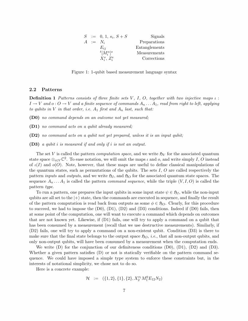


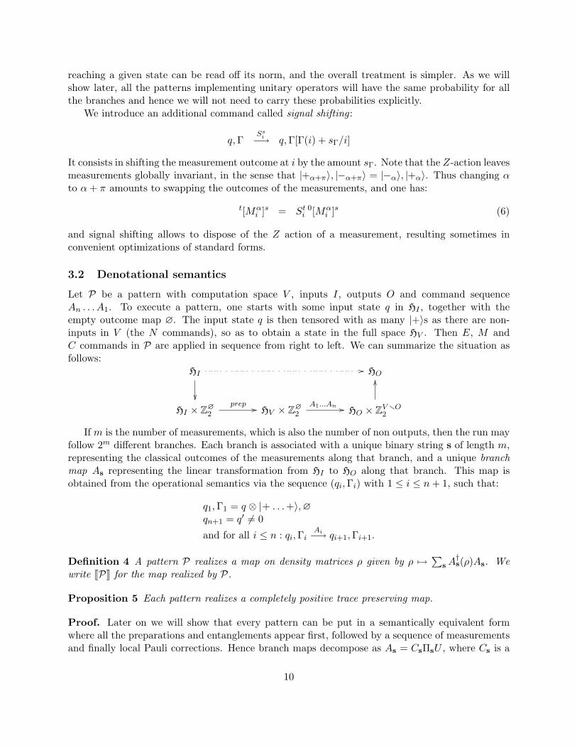


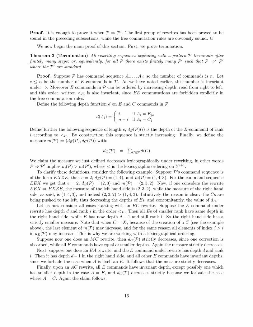


![Introduction to Measurement Statistics 1 - McGill University€¦ · Introduction to Measurement Statistics 3 i.e. ∑[y – i – y –]2 k-1 is an unbiased estimate of σ2 n i.e.](https://static.documents.pub/doc/80x56/5ec6b56046a10a59aa3cdc5f/introduction-to-measurement-statistics-1-mcgill-introduction-to-measurement-statistics.jpg)


