The Mini-Robot Kheperaas a Foraging Animate:

Synthesis and Analysis of Behaviour

A. Loffler

System Dynamics and Simulation - ED514Astrium GmbH, D-88039 Friedrichshafen

J. Klahold and U. Ruckert

System and Circuit Technology, Heinz Nixdorf Institute,Paderborn University, Furstenallee 11, D-33102 Paderborn

E-mail: klahold@hni.uni-paderborn.de

A. Loffler, J. Klahold, and U. Ruckert. The Mini-Robot Khepera as a Foraging Animate:Synthesis and Analysis of Behaviour. InProceedings of the 5th International Heinz NixdorfSymposium: Autonomous Minirobots for Research and Edutainment (AMiRE), volume 97 ofHNI-Verlagsschriftenreihe, pp. 93–130, 2001.

Abstract. The work presented in this paper deals with the development of a methodologyfor resource-efficient behaviour synthesis on autonomous systems. In this context, a defini-tion of a maximal problem with respect to the resources of a given system is introduced. Itis elucidated by means of an exemplary implementation of the solution to such a problemusing the mini-robot Khepera as the experimental platform. The described task consists ofexploring an unknown and dynamically changing environment, collecting and transportingobjects, which are associated with light-sources, and navigating to a home-base. The criticalpoint is represented by the accumulated positioning errors in odometrical path-integrationdue to slippage. Therefore, adaptive sensor calibration using a specific variant of Kohonen’salgorithm is applied in two cases to extract symbolic, e.g. geometric, information from thesub-symbolic sensor data, which is used to enhance position control by landmark mappingand orientation. In order to successfully handle the arising complex interactions, a heteroge-neous control-architecture based on a parallel implementation of basic behaviours coupledby a rule-based central unit is proposed.

1 Introduction

When considering autonomous mobile robots, small systems are preferred to resolve partialproblems applying a bottom up approach. They are relatively cheap and due to their small sizethe experimental environment stays small too. The restricted resources of such a system poseproblems, which should be seen as a challenge and turned into an advantage. The limits regard-ing energy (period of validity), computing power, memory capacities, actuators (manipulatorsof environment), and sensors enforce the development of efficient solutions to the consideredproblems. For that reason, mostly partial aspects are considered up to now [2], e.g. obstacleavoidance [6], edge following, or simple navigation tasks [8]. The gained knowledge and re-sults can be transferred onto large robots. However, the problem of integrating partial solutionsto work together efficiently still remains.

gripper

visionturret

base module

Figure 1. The mini-robot Khepera [14, 29] transporting a paper cube.

The focus of our research in the area of behaviour generation on autonomous systems followsthe principle of maximal economy: The task may be defined asto create maximal functionalitywith respect to a given system under the constraint of limited resources. In the context ofrobotics, a problem may be considered as being (weakly) maximal, if its solution requires theuse of all available sensor-resources and actuators of the system in question. The so calledDynamical Nightwatch’s Problem presented in [21] by Loffler et. al. for example, does fulfilthis criterion. This paper now describes substantial extensions to the work presented in theearlier article.

1.1 Presentation of the Experimental Platform

The experimental platform utilized is the mini-robot Khepera [14] with two additional turrets(Fig. 1). The base module has a height of 30 mm, a diameter of 55 mm, a mass of about 90 g andis equipped with a Motorola 68331 micro-controller (256 kByte RAM), two DC motors withincremental encoders, four Ni-Cd accumulators (4.8 V) for energy supply and eight infrared-proximity sensors (transmitters and receivers). The sensors may also be used for measuringthe infrared intensity of the ambient light (receivers only) in which case they are referred toas light-sensors. Moreover, various add-on turrets are available, two of which are applied inthe presented work: the gripper and the K213 vision turret (linear camera). The gripper may bemoved to 256 positions and has two states (open/closed). The vision turret has an opening angleof 36◦ with a resolution of 64 pixels with a resolution of 8 bit; its maximal update frequency is2 Hz. Due to the robot’s small size and easy operability, it represents a versatile tool for scientificinvestigation in the field of autonomous systems. For a historical review concerning both thedesign and the development of the mini-robot Khepera as well as the underlying motivation,please refer to article [28] by Mondada et. al. in [23].

transfer of calculatedmotor values

process 1 process 2 process 3 process 15

sensor - or respectively perception space

memorizedlandmarks

(type, position)

internal states(landmark detected,edge followed, etc.)

weighted input values

central control unit

output values (to actuators)

Figure 2. Schematic of the implementation concept, which assures the effi-

cient usage of the given system resources.

1.2 Design Methodology Used

The task to implement a solution to a maximal problem has led to the development of a par-ticularly adapted interaction concept (Fig. 2). The operating system of the Khepera allows theprocessing of up to 15 concurrent tasks. These tasks may represent the basic behavioural mod-ules (e.g. obstacle avoidance, edge following, etc.) which operate on a subset of the available,multidimensional sensor space (8 infrared-/light-sensors, 2 incremental encoders, etc.). Themotor values calculated by the respective basic modules are transferred to the central controlunit that makes decisions about their (weighted) interaction due to both input-data (e.g. currentsensor state) as well as internal states (e.g. memorized landmarks). The requests from the cen-tral module to transfer the calculated motor values occur in fixed time-intervals, which ensuresthe real-time capability of the system (if no new values are available, the old ones are taken).The update time is designed to maximize the number of program cycles which may be carriedout during the autonomy time, which is determined by the allocated energy resources. Further-more, the basic modules are designed in a simple and robust way, which does not overextendthe sensor-hardware’s range and precision and also guarantees fast data processing. Eventu-ally, only the locations of meaningful objects, e.g. landmarks, are memorized which limitsthe required storage capacities. The observation of this concept assures a resource-efficientimplementation. In this context, resource-efficiency may be defined as a Pareto-optimizationproblem: real-time capability has to be assured, the number of program cycles maximized(with respect to the available energy reserves) and the allocated memory minimized, whereby acorrect accomplishment of the envisaged task is assumed. Note that one program cycle corre-sponds to one situation that the robot has to master. Therefore, the objective is to successfullycope with a maximum number of situations. The resulting overall optimization task represents acomplex problem which cannot be solved analytically. Consequently, the illustrated interactionconcept has to be accompanied by a particular design cycle (Fig. 3) which closely couples thebehaviour synthesis, with various steps of analysis, leading to an iterative optimization of theprogram parameters. The behaviour synthesis is carried out using the bottom-up methodology,e.g. to succeedingly add new basic modules which entails the modification of the correspond-ing interaction schema (Fig. 2), and is constantly accompanied by simulations [26]. The appliedmethods are analysed by means of error propagation techniques whereby the sensor characteris-

errorcalculation

sensoranalysis

Visualisation ToolSimulator

parameter optimization

parameter optimization

adaption ofparameters

to the real case

real system/real environmentsensorcharac-teristics

transfer ofrecorded dataapplied

methods

comparison of performances

graphicaldata analysis

behavioursynthesis

Figure 3. The design cycle. Essential to the proposed concept is the close

coupling between behaviour synthesis and various analysis loops.

tics, on which the corresponding algorithms are based, are recorded with the real system. Bothlead to ana priori parameter optimization. After having carried out the real experiment, therecorded data are graphically analysed using a specially developed visualization tool describedin [19, 20]. This method may be applied to compare the performances of simulator solutionsand real cases as well as to further optimize, i.e. in ana posterioriway, the program parameters.

The applied methods concerning the behaviour generating modules can be classified into threebasic groups:Firstly, geometrical calculations have been applied for position control tasks. They include boththe odometrical path integration based on the incremental encoder values (‘step counters’) andthe landmark orientation processes. This has been done for two reasons: on the one hand theseproblems are of geometrical nature and on the other hand they are responsive to calculus oferror.Secondly, Braitenberg [1] neural networks have been used to create simple, but robust basicbehaviours like obstacle avoidance, edge following, etc. They have the advantage that, becauseof their reflexive nature, they do not require a high precision on the part of the sensor system.Moreover, they are not in conflict to the real-time demands due to their low complexity. Fur-thermore, a variant of Kohonen’s algorithm [25] has been applied for sensor preprocessing incases where accurate actions have to be carried out demanding a higher sensorial precision.Thirdly, concerning the central unit which controls the interactions of the various modules,rule-based reasoning has been applied. This has the advantage that higher, i.e. ‘cognitive-like’,decisions may be carried out. Note that in cases where more than one module may contributeto current actions, no explicit subsumption architecture as proposed by Brooks [2] is used, buta weighted superposition of the incoming motor values, which leads to the establishment of animplicit priority system.

1.3 Organization of the Paper

This paper is organized as follows: after giving an overview of related works in section 2,sections 3 to 6 describe the three parts of the developed algorithms in detail:

• Firstly, the position control by means of odometrical path integrating (section 3) andreflexive schemata (section 4) are investigated. These schemata—exploration and navi-gation [22] algorithms—are based on the positioning system. Their particularity resides

in the fact that the environment is supposed to be unknown and not static, i.e. they aresubjected to dynamical changes while the program is carried out.

• The second part describes a first approach to reduce the errors of the positioning sys-tem using additional sensor information. Therefore, section 5 gives an introduction to amethodology for adaptive sensor calibration [22], which allows to extract symbolic, i.e.geometrical, information from a sub-symbolic sensor data stream.

• The third part shows applications of the sensor calibration in two different cases (sec-tion 6). In the first one a local position correction is introduced and in the second, aglobal positioning system.

Eventually in section 7 the full-scale problem will be defined, the arising interactions discussedand the overall solution evaluated. The paper closes with a short conclusion (section 8).

2 Works Related to Our Approach

The related works discussed in this section have to be seen exemplary since they do not claim tobe complete and should only be regarded in relation to this work. It is broadly divided into thethree subsections—‘simulated vs. real experiments’, ‘behaviour synthesis utilizing the mini-robot Khepera’, ‘navigation techniques’—and concludes with a short classification of the workpresented in this paper.

2.1 Simulated vs. Real Experiments

De Sa et. al. [5] describes the (simulated) implementation of a controller comprising of threestages: the first level (reactive sensor-data processing) is realized by using a feedforward neuralnetwork, the second level (instinct-like manoeuvring) consists of pre-defined behaviour mod-ules which are selected by a fuzzy controller, and the third level (cognitive motion planning)steers the global behaviour through rule-based reasoning.

Prem [32], on the one hand, extensively discusses the aspect of embodiment (embedding thecontroller into a real robot) which is especially crucial for hardware realisations of autonomousagents. On the other hand, Pipe et. al. [31] quantitatively analyze the learning performance ofautonomous systems on the basis of simulations, concerning so-called cognitive maps under theassumption that senor and motor values are subjected to noise.

Miglino et. al. [27] presents results regarding the transfer of evolutionary developed controllersto real robots. This is particularly interesting in the context of genetic algorithms and similartechniques, because of the fact that generally a high number of evolution cycles have to becarried out to obtain viable results. This categorically forbids the use of a real system duringthe process of evolution. It is shown that an accurate model of the robot can be obtained,if real sensor characteristics are included, and that the introduction of conservative noise intothe evolutionary process considerably smooths the transition to the real system, which—aftercarrying out some additional evolution cycles—shows the same performance as the simulatedone.

Jakobi [13] contributes substantially to the ongoing discussion concerning the transfer of simu-lated controllers to real autonomous systems by developing the concept of the so-called minimal

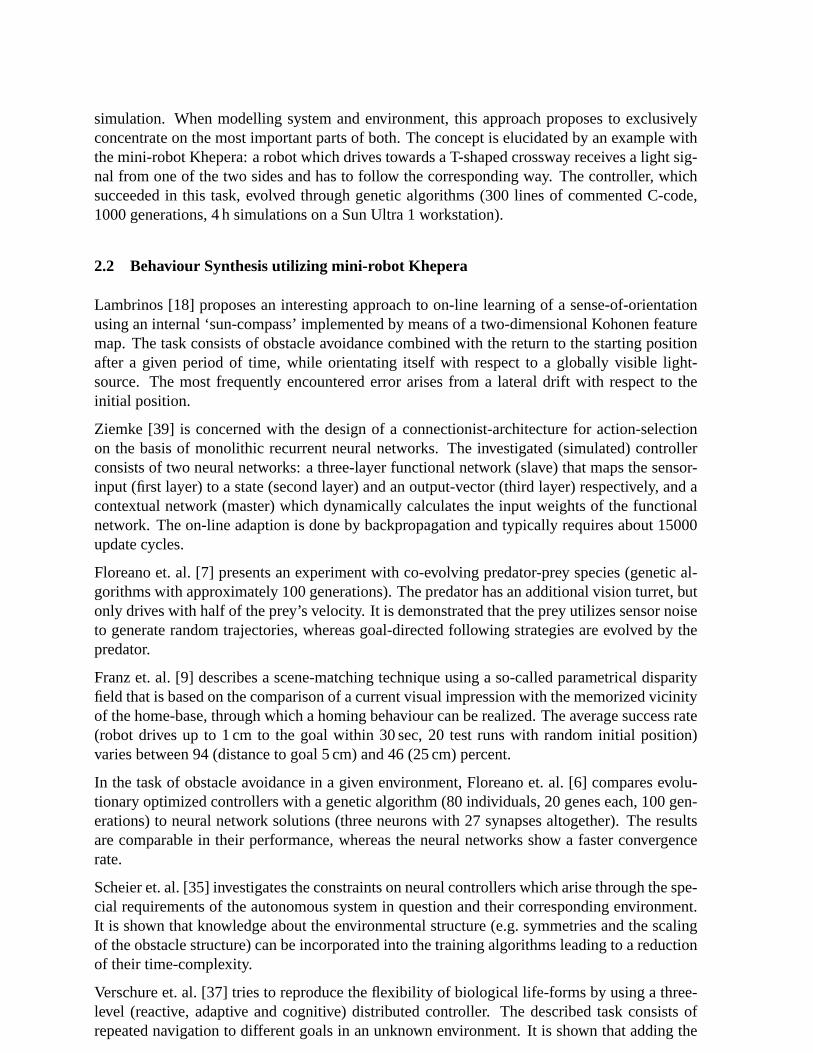
simulation. When modelling system and environment, this approach proposes to exclusivelyconcentrate on the most important parts of both. The concept is elucidated by an example withthe mini-robot Khepera: a robot which drives towards a T-shaped crossway receives a light sig-nal from one of the two sides and has to follow the corresponding way. The controller, whichsucceeded in this task, evolved through genetic algorithms (300 lines of commented C-code,1000 generations, 4 h simulations on a Sun Ultra 1 workstation).

2.2 Behaviour Synthesis utilizing mini-robot Khepera

Lambrinos [18] proposes an interesting approach to on-line learning of a sense-of-orientationusing an internal ‘sun-compass’ implemented by means of a two-dimensional Kohonen featuremap. The task consists of obstacle avoidance combined with the return to the starting positionafter a given period of time, while orientating itself with respect to a globally visible light-source. The most frequently encountered error arises from a lateral drift with respect to theinitial position.

Ziemke [39] is concerned with the design of a connectionist-architecture for action-selectionon the basis of monolithic recurrent neural networks. The investigated (simulated) controllerconsists of two neural networks: a three-layer functional network (slave) that maps the sensor-input (first layer) to a state (second layer) and an output-vector (third layer) respectively, and acontextual network (master) which dynamically calculates the input weights of the functionalnetwork. The on-line adaption is done by backpropagation and typically requires about 15000update cycles.

Floreano et. al. [7] presents an experiment with co-evolving predator-prey species (genetic al-gorithms with approximately 100 generations). The predator has an additional vision turret, butonly drives with half of the prey’s velocity. It is demonstrated that the prey utilizes sensor noiseto generate random trajectories, whereas goal-directed following strategies are evolved by thepredator.

Franz et. al. [9] describes a scene-matching technique using a so-called parametrical disparityfield that is based on the comparison of a current visual impression with the memorized vicinityof the home-base, through which a homing behaviour can be realized. The average success rate(robot drives up to 1 cm to the goal within 30 sec, 20 test runs with random initial position)varies between 94 (distance to goal 5 cm) and 46 (25 cm) percent.

In the task of obstacle avoidance in a given environment, Floreano et. al. [6] compares evolu-tionary optimized controllers with a genetic algorithm (80 individuals, 20 genes each, 100 gen-erations) to neural network solutions (three neurons with 27 synapses altogether). The resultsare comparable in their performance, whereas the neural networks show a faster convergencerate.

Scheier et. al. [35] investigates the constraints on neural controllers which arise through the spe-cial requirements of the autonomous system in question and their corresponding environment.It is shown that knowledge about the environmental structure (e.g. symmetries and the scalingof the obstacle structure) can be incorporated into the training algorithms leading to a reductionof their time-complexity.

Verschure et. al. [37] tries to reproduce the flexibility of biological life-forms by using a three-level (reactive, adaptive and cognitive) distributed controller. The described task consists ofrepeated navigation to different goals in an unknown environment. It is shown that adding the

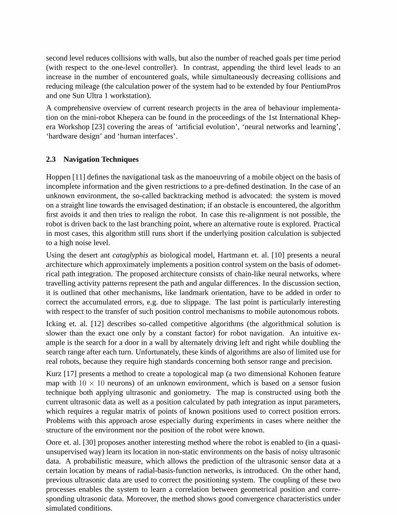
second level reduces collisions with walls, but also the number of reached goals per time period(with respect to the one-level controller). In contrast, appending the third level leads to anincrease in the number of encountered goals, while simultaneously decreasing collisions andreducing mileage (the calculation power of the system had to be extended by four PentiumProsand one Sun Ultra 1 workstation).

A comprehensive overview of current research projects in the area of behaviour implementa-tion on the mini-robot Khepera can be found in the proceedings of the 1st International Khep-era Workshop [23] covering the areas of ‘artificial evolution’, ‘neural networks and learning’,‘hardware design’ and ‘human interfaces’.

2.3 Navigation Techniques

Hoppen [11] defines the navigational task as the manoeuvring of a mobile object on the basis ofincomplete information and the given restrictions to a pre-defined destination. In the case of anunknown environment, the so-called backtracking method is advocated: the system is movedon a straight line towards the envisaged destination; if an obstacle is encountered, the algorithmfirst avoids it and then tries to realign the robot. In case this re-alignment is not possible, therobot is driven back to the last branching point, where an alternative route is explored. Practicalin most cases, this algorithm still runs short if the underlying position calculation is subjectedto a high noise level.

Using the desert antcataglyphisas biological model, Hartmann et. al. [10] presents a neuralarchitecture which approximately implements a position control system on the basis of odomet-rical path integration. The proposed architecture consists of chain-like neural networks, wheretravelling activity patterns represent the path and angular differences. In the discussion section,it is outlined that other mechanisms, like landmark orientation, have to be added in order tocorrect the accumulated errors, e.g. due to slippage. The last point is particularly interestingwith respect to the transfer of such position control mechanisms to mobile autonomous robots.

Icking et. al. [12] describes so-called competitive algorithms (the algorithmical solution isslower than the exact one only by a constant factor) for robot navigation. An intuitive ex-ample is the search for a door in a wall by alternately driving left and right while doubling thesearch range after each turn. Unfortunately, these kinds of algorithms are also of limited use forreal robots, because they require high standards concerning both sensor range and precision.

Kurz [17] presents a method to create a topological map (a two dimensional Kohonen featuremap with10 × 10 neurons) of an unknown environment, which is based on a sensor fusiontechnique both applying ultrasonic and goniometry. The map is constructed using both thecurrent ultrasonic data as well as a position calculated by path integration as input parameters,which requires a regular matrix of points of known positions used to correct position errors.Problems with this approach arose especially during experiments in cases where neither thestructure of the environment nor the position of the robot were known.

Oore et. al. [30] proposes another interesting method where the robot is enabled to (in a quasi-unsupervised way) learn its location in non-static environments on the basis of noisy ultrasonicdata. A probabilistic measure, which allows the prediction of the ultrasonic sensor data at acertain location by means of radial-basis-function networks, is introduced. On the other hand,previous ultrasonic data are used to correct the positioning system. The coupling of these twoprocesses enables the system to learn a correlation between geometrical position and corre-sponding ultrasonic data. Moreover, the method shows good convergence characteristics undersimulated conditions.

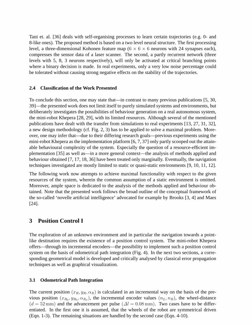
Tani et. al. [36] deals with self-organising processes to learn certain trajectories (e.g. 0- and8-like ones). The proposed method is based on a two level neural structure. The first processinglevel, a three-dimensional Kohonen feature map (6 × 6 × 6 neurons with 24 synapses each),compresses the sensor data of a laser scanner. The second, a partly recurrent network (threelevels with 5, 8, 3 neurons respectively), will only be activated at critical branching pointswhere a binary decision is made. In real experiments, only a very low noise percentage couldbe tolerated without causing strong negative effects on the stability of the trajectories.

2.4 Classification of the Work Presented

To conclude this section, one may state that—in contrast to many previous publications [5, 30,39]—the presented work does not limit itself to purely simulated systems and environments, butdeliberately investigates the possibilities of behaviour generation on a real autonomous system,the mini-robot Khepera [28, 29], with its limited resources. Although several of the mentionedpublications have dealt with the transfer from simulations to real experiments [13, 27, 31, 32],a new design methodology (cf. Fig. 2, 3) has to be applied to solve a maximal problem. More-over, one may infer that—due to their differing research goals—previous experiments using themini-robot Khepera as the implementation platform [6, 7, 37] only partly scooped out the attain-able behavioural complexity of the system. Especially the question of a resource-efficient im-plementation [35] as well as—in a more general context—the analysis of methods applied andbehaviour obtained [7, 17, 18, 36] have been treated only marginally. Eventually, the navigationtechniques investigated are mostly limited to static or quasi-static environments [9, 10, 11, 12].

The following work now attempts to achieve maximal functionality with respect to the givenresources of the system, wherein the common assumption of a static environment is omitted.Moreover, ample space is dedicated to the analysis of the methods applied and behaviour ob-tained. Note that the presented work follows the broad outline of the conceptual framework ofthe so-called ‘novelle artificial intelligence’ advocated for example by Brooks [3, 4] and Maes[24].

3 Position Control I

The exploration of an unknown environment and in particular the navigation towards a point-like destination requires the existence of a position control system. The mini-robot Kheperaoffers—through its incremental encoders—the possibility to implement such a position controlsystem on the basis of odometrical path integration (Fig. 4). In the next two sections, a corre-sponding geometrical model is developed and critically analysed by classical error propagationtechniques as well as graphical visualization.

3.1 Odometrical Path Integration

The current position(xR, yR, αR) is calculated in an incremental way on the basis of the pre-vious position(xR0 , yR0 , αR0 ), the incremental encoder values(nL, nR), the wheel-distance(d = 52 mm) and the advancement per pulse(∆l = 0.08 mm). Two cases have to be differ-entiated. In the first one it is assumed, that the wheels of the robot are symmetrical driven(Eqn. 1-3). The remaining situations are handled by the second case (Eqn. 4-10).

|∆n|=1

x0 x

y

y0

r

∆l × n R

∆l × n L

d

rotation point

x-axis

y-axis

αR0

∆αR∆αR

αR0

αR

Figure 4. Graphical representation of the position calculation by path inte-

gration showing the current and the previous position.

1. case:|nL| = |nR|

αR = αR0 + (nR − nL)∆l

d(1)

xR = xR0 +nR + nL

2∆l cos(αR) (2)

yR = yR0 +nR + nL

2∆l sin(αR) (3)

2. case:|nL| 6= |nR|

∆αR =

∣∣∣∣(|nR| − sign(nRnL) |nL|) ∆l

d

∣∣∣∣ (4)

r =

∣∣∣∣∣( |nR|+ |nL||nR| − |nL|

)sign(nRnL)d

2

∣∣∣∣∣ (5)

∆xR = r − r cos(∆αR) (6)

∆yR = r sin(∆αR) (7)

xR = xR0 + sign(nR + nL)∆yR cos(αR0) + ∆xR cos(αR0 + sign (|nR| − |nL|) π

2

)(8)

yR = yR0 + sign(nR + nL)∆yR sin(αR0) + ∆xR sin(αR0 + sign (|nR| − |nL|) π

2

)(9)

αR = αR0 + ∆αR sign (nR − nL) (10)

−100−50

050

100

−100−50

050

100

0.08

0.0804

0.0808

nLnR

posi

tion

erro

r F

[mm

]

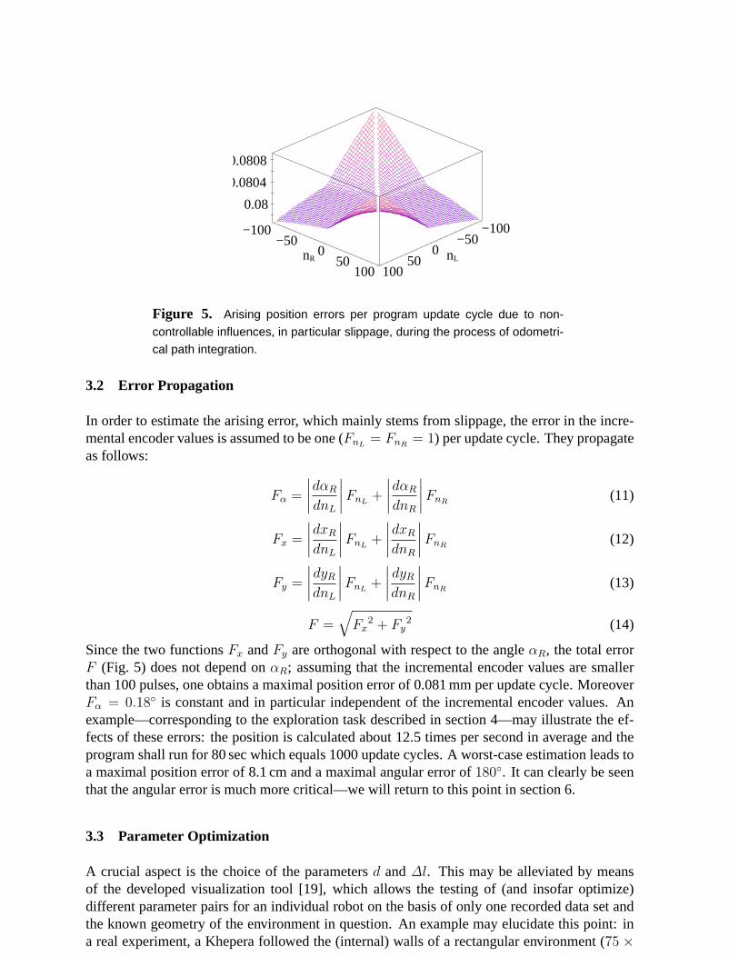
Figure 5. Arising position errors per program update cycle due to non-

controllable influences, in particular slippage, during the process of odometri-

cal path integration.

3.2 Error Propagation

In order to estimate the arising error, which mainly stems from slippage, the error in the incre-mental encoder values is assumed to be one (FnL

= FnR= 1) per update cycle. They propagate

as follows:

Fα =

∣∣∣∣dαR

dnL

∣∣∣∣FnL+

∣∣∣∣dαR

dnR

∣∣∣∣ FnR(11)

Fx =

∣∣∣∣dxR

dnL

∣∣∣∣ FnL+

∣∣∣∣dxR

dnR

∣∣∣∣ FnR(12)

Fy =

∣∣∣∣dyR

dnL

∣∣∣∣FnL+

∣∣∣∣dyR

dnR

∣∣∣∣FnR(13)

F =√

Fx2 + Fy

2 (14)

Since the two functionsFx andFy are orthogonal with respect to the angleαR, the total errorF (Fig. 5) does not depend onαR; assuming that the incremental encoder values are smallerthan 100 pulses, one obtains a maximal position error of 0.081 mm per update cycle. MoreoverFα = 0.18◦ is constant and in particular independent of the incremental encoder values. Anexample—corresponding to the exploration task described in section 4—may illustrate the ef-fects of these errors: the position is calculated about 12.5 times per second in average and theprogram shall run for 80 sec which equals 1000 update cycles. A worst-case estimation leads toa maximal position error of 8.1 cm and a maximal angular error of180◦. It can clearly be seenthat the angular error is much more critical—we will return to this point in section 6.

3.3 Parameter Optimization

A crucial aspect is the choice of the parametersd and∆l. This may be alleviated by meansof the developed visualization tool [19], which allows the testing of (and insofar optimize)different parameter pairs for an individual robot on the basis of only one recorded data set andthe known geometry of the environment in question. An example may elucidate this point: ina real experiment, a Khepera followed the (internal) walls of a rectangular environment (75 ×

∆l[mm] 0.076 0.077 0.078 0.079 0.080∆α[◦] 18.6 9.4 0.1 -9.1 -18.3

∆l[mm] 0.081 0.082 0.083 0.084∆α[◦] -27.6 -36.8 -46.0 -55.2

Table 1. Final angular error ∆α with respect to variation of ∆l (original con-

figuration: bold).

d[mm] 48 49 50 51 52∆α[◦] -79.8 -63.5 -47.9 -32.81 -18.3

d[mm] 53 54 55 56∆α[◦] -4.4 9.0 21.9 34.4

Table 2. Final angular error ∆α with respect to variation of d (original config-

uration: bold).

obstacle avoidance

drift

turning

edge following

Figure 6. The interaction structure incorporating both the basic schemata re-

sponsible for the exploration of an unknown environment (without drift schema)

as well as the point-to-point navigation to a destination of known position (in-

cluding the drift schema).

60 cm) for roughly two rounds (i.e. 92 sec corresponding to 1126 program cycles) and stoppedat an internal angle of71.7◦ instead of the expected90◦. Tables 1 and 2 show the obtained finalangular values with respect to variations ofd and∆l respectively, where the original values(d = 52 mm,∆l = 0.08 mm) have been averaged over four different robots. From these data,one may conclude that the parameter pairs (d = 52 mm,∆l = 0.078 mm or d = 53 mm,∆l =0.08 mm respectively) would have been better suited for the tested robot.

4 Exploration and Navigation

Exploration and navigation in unknown and potentially changing environments represent one ofthe basic and most intriguing problems concerning mobile autonomous robots. The most impor-tant constraints reside in the limited energy resources of such a system limiting its autonomytime, the real-time demands, the restricted calculation power, memory capacities and sensorrange and precision. These severe constraints motivate the development of simple, but robustbasic schemata with limited absolute time complexity. Moreover, the unknown and changingnature of the environment entails the use of heuristics as well as avoiding explicit maps for threereasons: the environment is non-static, the position control is subjected to considerable errors

0

200

400

600

800

1000

1200

0 5 10 15 20 25 30 35 40 45 50

sens

or v

alue

distance to obstacle [mm]

average valueminimal value

maximal value

∆ ≈ 100

0

0.5

1

1.5

2

2.5

3

3.5

4

0 5 10 15 20 25 30 35 40 45 50

stan

dard

dev

iatio

n

distance to obstacle [mm]

Figure 7. The distance characteristic (left) of the infrared sensors on the

robot (sensor S2, middle left) and the corresponding standard deviation (right),

whereby the mean value has been taken from 50 samples.

and the available memory capacities are severely constricted. The exploration and navigationconcept developed, incorporates the four basic modules of obstacle avoidance, edge following,drift and turning, whose interaction schema is depicted in Fig. 6. Thereby the motor outputvalues of edge following (respectively drift) and obstacle avoidance are superimposed, whereinthe obstacle avoidance has an implicit priority and also provides the basic propulsion. Eventu-ally, in cases where turning on the spot is necessary, the schema turning suppresses the otherones. Before describing the developed algorithms, ana priori analysis of the infrared proximitysensors is presented, on which all of the algorithms in the current section rely.

4.1 Analysis of the Infrared Proximity Sensors

The recorded characteristics of the infrared proximity sensors and corresponding standard devi-ation (Fig. 7) show that the proximity sensitivity is limited to an interval from approximately 1.7to 3.3 cm. Moreover, the maximal, respectively minimal values are shown, which may differ by∆ ≈ 100. For distances smaller than 1.7 cm the sensors saturate and above 3.3 cm only noise isdetectable, which is caused by the quantization. Relating this to the system’s diameter (5.5 cm),one realizes that the robot has to carry out its exploration task with a sensing system restrictedto local perception. Moreover, despite the fact that the standard deviation with about 3 impulsesseems to be quite low, the algorithms have to be designed in such a way that a noise level of 50impulses can be tolerated.

Eventually, on the basis of the recorded sensor characteristics, a model for the visualizationtool was developed (Fig. 8 left). The scalar sensor values are transformed to areas in whichan obstacle may be located (Fig. 8 right). The thickness of the characteristics represents thecorresponding noise level. This sensor model may be utilized for the process ofa posteriorigraphical analysis, thereby reconstructing the system’s perception of its environment (Fig. 9).The reconstruction consists of two steps; first the accumulated sensor characteristics are drawn(Fig. 9 middle), and then the parts the robot travelled across are erased to correct the view (Fig. 9right). The real environment (Fig. 9 left) is given as reference.

Figure 8. The scalar sensor values are—by means of the adjustable angu-

lar characteristics (left)—transformed to areas in which an obstacle may be

located (right).

4.2 Obstacle Avoidance

Obstacle avoidance is one of the most basic tasks for mobile autonomous robotics. The pre-sented algorithm is inspired by Braitenberg’s vehicle IIIb [1] and also provides the basic propul-sion. The velocity reduction of the right motor due to an obstacle on the left (Fig. 10 left) isrepresented by the dashed arrow. In order to get the relationship betweendistance-to-obstacleand speed, The activation function of the neurons (Fig. 10 right) has to be superimposed onthe sensor characteristic (Fig. 7). The right (respectively the left) front sensors’ values and thecorresponding weight vector (w0 = w5 = 0, w1 . . . w4 = 1/2) are multiplied by means of thedot product and transferred in an inhibitory way to the opposite motor. The initialization ofthe weights may be considered as a sensitivity function; the factw0 = w5 = 0 is necessary toguarantee a smooth interaction with the edge following algorithm (see below). Moreover, theactivation function of the two neurons represents a modified step function (the threshold is ran-domly chosen to be475± 25, which avoids the formation of a preference direction) combinedwith a proportionality relation, permitting a smoother driving behaviour.

4.3 Edge Following

The edge following algorithm enables the system to leave room-like substructures of the en-vironment in a time-efficient way. The basic concept consists of keeping the distance-to-wall

Figure 9. On the basis of the sensor model it is possible to regain a notion

of the perceived environmental structure.

w0

w1w2 w3w4

w5

S0

S1

S2 S3S4

S5

-8

-6

-4

-2

0

2

4

6

8

0 200 400 600 800 1000

thresholds

net-input of the neuron

mot

or o

utpu

t

Figure 10. Representation of the neural network that implements the ob-

stacle avoidance behaviour (left) with the activation function of the neurons

(right).

(a)

(b)

(c)

S0 S0S0

Figure 11. Behaviour implemented during the edge following algorithm.

constant, i.e. to implement a control system which keeps the sensor valueS0 (resp.S5) constant.Thereby three different situations may occur (Fig. 11):

a) driving along a newly found wall (the sensor valueS0 will be memorized);

b) approaching a wall if the robot has drifted away (current sensor value is lower than thememorized one);

c) the robot drives away from the wall by means of the obstacle avoidance schema.

Moreover, a neural interpretation of the edge following algorithm is shown in Fig. 12. Therein aneuron, represented by a circle, calculates the sum of its input values, represented by incomingarrows, if not specified otherwise. If the difference of the current to the previous sensor valueis smaller than a noise discriminating threshold of−7 and is detected, a drift value of−1 is

outerIR-sensor S0(t)

drift: -1 wall lost,drift: ±8

-S0(t-1)

Reset:S0(t-1) := 0Smem := 0

memorizing:Smem := -S0(t)

l. MN backwards forwards

nomemorizing

r. MNl. MN

< -7

> 7

cycles< -100

> 120

backwards

Τ

Figure 12. Neural interpretation of the edge following algorithm (the wall is

assumed to be on the left side of the robot; l./r. MN = left-/right motor neuron).

target

direction to target

corresponds to 10 pulses/10mscorresponds to 8 pulses/10mscorresponds to 6 pulses/10mscorresponds to 2 pulses/10ms

angular area in which the drift acts on both motorsangular area in which the drift acts on only one motorangular area in which the drift is not active

Figure 13. Representation of the effects of the drift schema depending on

the angular miss-alignment.

superimposed on the left motor. If the difference is greater than7 (approximately twice thestandard deviation), i.e. the robot is approaching the wall, the current sensor value will bememorized (Smem = −S0(t)). In case the robot loses the wall (S0(t)+Smem < −100), a strongcurve towards the wall will be driven until either the wall is relocated (Smem = −S0(t)) or 120program cycles have been carried out. The edge following process starts with a reset.

4.4 Drift

The drift schema in conjunction with the obstacle avoidance and the turning algorithm (whichmay be considered as a special case of the drift schema) enables the robot to navigate to a pointof known coordinates. Note that—for the discussed reasons—no map of the environment isavailable, e.g. no optimal path may be calculated; in consequence, this schema tries to manoeu-vre the robot towards its destination on a straight line. An initial turn on the spot (Fig. 14 (1))orientates the robot towards its navigational destination. If, during the process of manoeuvringtowards this destination an obstacle is encountered (2), it will be avoided and the system willtry to reorientate itself (3) by superimposing an adequate drift with respect to the angular miss-alignment (Fig. 13). Moreover, in order to avoid cyclic movements, the nearest point reached is

target(tolerance area)

4

3

1 2

Figure 14. Example of a navigation sequence.

l. MN

DemandValue α0

InternalSensor α

weakstrong

α0-αα0-α

memorize:closest position

current position

diff3×

r. MN

Figure 15. Neural structure that implements the drift (Fig. 13) as well as the

turning schemata (Fig. 16).

memorized; in case this point is reencountered for the second time (with a tolerance of 5 cm),the drift is halved which leads to wider movements permitting the robot to leave small envi-ronmental substructures. If this still leads to cyclic behaviour, the navigation algorithm will beinterrupted for a fixed (but increasing with the number of failures) number of program cycles inorder to search a new starting point, which in practice amounts to an edge following behaviour.Finally, if the robot has approached its target by 15 cm (Fig. 14 (4)), a turn on the spot to reori-entate the system is carried out and the basic propulsion is halved, avoiding an ‘overshot’. Incase the target is reached within 5 cm, the task is considered to be completed. This tolerancearea concerning both target and nearest-point-reached is introduced due to the errors stemmingfrom the path integration process. Eventually, the drift schema may also be interpreted in aneural way (Fig. 15).

4.5 Turning

The presented structure for implementing the drift schema (Fig. 15) may also be utilized torealize a turning-on-the-spot algorithm, where only the thresholds as well as the switch betweena strong and a weak drift cease to exist. The resulting behaviour together with a visualizationfor two criteria causing a turn of180◦ are shown in (Fig. 16).

0 1 2 3 4 5

0 1 2 3 4 5

Figure 16. If it is not possible to leave a pre-defined circle during a given

number of program cycles (left) or if its front IR-sensors perceive certain char-

acteristical patterns (right), the robot performs a 180◦ turn.

0

200

400

600

800

1000

0 200 400 600 800 1000

y [m

m]

x [mm]

path

A B

strong drift

weak driftinterception ofthe algorithm

reorientation

0

100

200

300

400

500

-300-200-100 0 100 200 300

y [m

m]

x [mm]

path

A

B

Figure 17. Trajectory of the robot during the A-to-B-navigation process in a

simulated (left) and a real (right) environment.

4.6 Results: Point-to-Point Navigation

Concerning the simulator (Fig. 17 left), the developed navigation algorithm shows a very goodbehaviour in case of ‘open’ environments, i.e. structures without narrow, maze-like obstaclearrangements, for which the chosen parameter set is not adapted. This example (Fig. 17 left)points out the different drift factors (strong/weak) as well as the interception of the algorithmand the reorientation in the vicinity of the target. In the real case (Fig. 17 right), a comparableperformance may be achieved on a smaller scale. Although a particularly harsh structure (twosuccessive dead ends) was chosen, the robot reached the envisaged target with a deviation of∆x = 2 cm and∆y = 1 cm which is well inside the tolerance area.

It is nevertheless obvious that the proposed navigation algorithm is heavily dependent on theunderlying position calculation. For this reason, the next two sections will see the introductionof a technique for adaptive sensor calibration and its application to enhance the positioningsystem.

5 Adaptive Sensor Calibration

Adaptive sensor calibration provides a means by which two different goals may be achieved: onthe one hand, it allows the extraction of symbolic information from the generally sub-symbolic

t1

t2

t0

adaption range

lear

ning

rat

e

input values associated output value

Figure 18. Schematic of a 1-dimensional self organising map (SOM) during

the training period.

sensor data, and on the other hand, the quite intriguing problem of varying responses of indi-vidual sensors to identical circumstances, due to fabrication tolerances, may be approached. Inthe context of the presented work, a methodology on the basis of a variant of Kohonen’s algo-rithm [16] inspired by Malmstroem et. al. [25] is used to extract geometrical informations fromhigh dimensional sensor data in two cases: the calibration of the light-sensors leads to an angle-to-light-source value and the calibration of the linear camera provides distance-to-landmarkinformation. First of all, the underlying algorithm shall be briefly explained.

5.1 Description of the Algorithm

The basic idea consists of approximating a function f which maps an n-dimensional input vectoronto an m-dimensional output vector by classifying the input vectors, wherein a particular out-put vector is associated with every class. In the following, the output will be a scalar value dueto the particular structure of the encountered problems; please note however, that the presentedmethodology is not restricted to this case.

f : Rn −→ Rm , here m = 1 (15)

The methodology is divided into a training and a recall phase. In the training phase, it is as-sumed that a suitable data set is available (either by previous recording or by on-line input)which consists of example vectors containing both the sensorial data (~s) as well as the associ-ated output value (o). The network consists of k randomly initialised neurons which match theexample vectors regarding their dimensions. Moreover, they have fixed locations, i.e. it is as-sumed that the vectori is adjacent to the vectorsi−1 andi+1, which results in a 1-dimensionalstructure being the most appropriate for the investigated cases. Again this does not representa principal restriction; on the contrary, the dimension of the network should be adapted to thedimension of the output vector in question, which considerably simplifies the visualization ofthe results.

50

100

150

200

250

300

350

400

450

500

0 50 100 150 200 250 300se

nsor

val

ue

distance to light-source [mm]

Figure 19. Characteristic curve of the light-sensors.

During the training phase, the neuron with the minimal distance to the current example vector(Eqn. 16) is determined (best match) and all neurons (Eqn. 17) are adapted towards the example(Eqn. 18, 19), whereby the adaption strengthλ is dependent on the distance of the neuron inquestion to the best match. Moreover, the adaption strength decreases in time which leads toa quick but coarse ordering in an early phase of the training process and fine-tuning later on.In the given example (Fig. 18) the triangles represent the various learning rates and adaptionranges at different times (t0 < t1 < t2). The marked neuron represents the best match, whichmeans the neuron with the weight vector closest to the input vector. The vectors contain theinput values and the corresponding output value associated by training. The training phase endswhen no further decrease of the classification error can be detected. Note that the number ofneurons utilized is dependent on the requirements of the application in question.

~Vex = (s0 . . . sn, o) (16)

~Vi = (~wi, ϕi) (17)

mini=1...k

∥∥∥~Vi − ~Vex

∥∥∥ ⇒ ~Vbm (18)

~Vi(t + 1) = ~Vi(t) + λ (t, |i− bm|) ~Vbm(t) (19)

During the recall phase, only the sensorial data (Eqn. 20) is available to the system; conse-quently, the best-match search is carried out considering only the first n components of thenetwork vectors. The complementary part associated with this best-match represents the re-quired output (Eqn. 21), i.e. the complete n+m-dimensional information is recovered by meansof a classification restricted to a n-dimensional subspace.

~sre = (s0 . . . sn) (20)

mini=1...k

‖~wi − ~sre‖ ⇒ ~wbm ⇒ f(~sre) = ϕbm (21)

5.2 Analysis of the Light-Sensors

The light-sensors (passively) measure the intensity of the infrared part of the ambient light. Acharacteristic, which has been obtained by a single measurement, is shown in (Fig. 19); thesensor value decreases with increasing intensity, i.e. decreasing distance to the light-source.When using a light-source with different intensity, the curve will be spread or compressed. In

12 3 4 5

6

ϕ

0 1 2 3 4 5

maximum value

Figure 20. Schematic of a 1-dimensional self-organizing neural network

which is used to extract a symbolic angle-to-light-source information (left) from

the sub-symbolic sensor stream (right). Note that the sensor values are in-

verted (Fig. 19).

0

100

200

300

400

500

−100 −50 0 50 100

sens

or v

alue

angle [°]

sensor 0sensor 1sensor 2sensor 3sensor 4sensor 5

Figure 21. Set of sensor values used for training the neural network.

this context, it should be noted that the measured characteristic depends on the intensity ofthe light-source in relation to the background infrared radiation, which prompts one to use thelight-sensors in a way which is independent of absolute intensity values. Furthermore, onemay artificially create ‘events’, such as for example ‘light-source encountered’, by introducingcorresponding intensity thresholds (dashed lines in Fig. 19), which have to be initially adaptedto the background radiation. Note that noise plays a significantly lesser role here as for the(active) proximity sensors.

5.3 Calibration of the Light-Sensors

Fig. 20 shows in a schematic way the task of the light-sensor network which consists of trans-forming the 6-dimensional intensity signal to 1-dimensional angular information. For the train-ing phase, a data set is obtained by placing a robot at a distance of 1 cm (4 cm for the test dataset) to a light-source and rotating it by180◦ while recording both sensor vectors (Fig. 21) andthe associated angle. The latter has been obtained by odometrical path integration on the basisof the incremental encoders. In order to take the significant distance dependence into account,a scaling operation is performed (Fig. 22) prior to training and recall. This operation scales the

0

100

200

300

400

500

−100 −50 0 50 100

sens

or v

alue

angle [°]

normalscaled

Figure 22. Set of values from sensor S3 in a quadruplicate distance to the

light-source with respect to the one the SOM was trained with.

−100

−80

−60

−40

−20

0

20

40

60

80

100

−100−80−60−40−20 0 20 40 60 80 100

ange

l fro

m a

ctiv

Neu

ron

[°]

angle to light−source [°]

optimal

testlearned

Figure 23. Result of the training, showing the test of the neural network

with the data set used for learning (fat dotted line) and respectively with a data

set resulting from a quadruplicate distance to the light-source (thin solid line).

As reference a straight line is drawn. In spite of the scaling, a large distance

sensitivity may be recognized.

sensor values, so that one of the six values has the normed lowest amount (50) and another onehas the normed highest amount (500). This is more advantageous than performing a normali-sation because of the border effects induced by the non-isotropic sensor arrangement (Fig. 20left).

The chosen network consists of 60 neurons and has been adapted in 20 cycles while reducingthe adaption width from 10 to 1 and the learning rate from 0.6 to 0.1 (Fig. 23). The averageerror amounts to the expected 1.52 degrees (the 60 neurons are distributed over the180◦ witha spacing of3◦). In contrast, the maximum error of6.52◦, occurring at the borders due to thenon-isotropic sensor arrangement. Despite the scaling operation, a strong distance sensitivityremains, which allows one to use the obtained network only at an optimal ‘working’ inten-sity. Using the visualization tool the current output of the network can be eventually displayed(Fig. 24).

Figure 24. Visualization of the trained neural network for the light-sensor

calibration.

36°

4.8 cm

lV

Figure 25. Schematic illustrating the recognition of a cylinder as a landmark

using the linear camera.

5.4 Vision Data Preprocessing

The calibration of the linear camera provides distance information with respect to a particularcylindrical landmark (Fig. 25). In order to reduce the data dimensionality (64 pixel with a reso-lution of 8 bit), a preprocessing is carried out. Firstly, a gradientGi of the original imageBi iscalculated (Eqn. 22) and subjected to a noise suppressing threshold (Eqn. 23), which allows thedetection of the right and left edges of the object, thereby permitting the identification of thelandmark.

Gi = Bi −Bi+1 (22)

|Gi| < 20 → Gi = 0 (23)

The result of this operation on a typical image is shown in (Fig. 26). Every image is the averageof 10 recordings; if in at least 4 recordings the system fails to identify two edges, the processis stopped. Moreover, Fig. 27 shows that next to the width of the perceived object, the minimalpixel value also carries some distance information, whereas the gradient values at the edgesare subjected to too much noise and the maximal value saturates at small distances. Therefore,width and minimal values are chosen to be the sensorial input variables. Note that due to thediameter of the utilized landmarks (about 4.8 cm) and the opening angle of the camera(36◦),a minimal operating distance of 10 cm is necessary; above 40 cm, the resolution of the cameradoes not permit a viable operation either.

0

50

100

150

200

250

0 10 20 30 40 50 60

grey

tone

pixel

centreleft edge

right edge

-60

-40

-20

0

20

40

60

80

100

0 10 20 30 40 50 60

grey

tone

dif

fere

nce

pixel

thresholds

right edge

left edge

Figure 26. Picture of a landmark in view of the robot as sub-symbolic vision

data (left) and the resulting gradient picture (right).

0

50

100

150

200

250

300

0 100 200 300 400 500 600 700 800

inpu

t val

ue

distance lV [mm]

width

maximumleft edge

right edgeminimum

width

max.

edges

min.

Figure 27. Diagram of several characteristics of the sub-symbolic vision

data.

5.5 Calibration of the Linear Camera

Due to the fact that only two input components and one output value are present in this example,the calibration of the linear camera appears suitable for a comparison between off-line andon-line training. A network consisting of 100 neurons has been trained in both cases withonly three cycles decreasing the adaption width from 10 to 1 and the learning rate from 0.8to 0.1. The on-line training required an initialization with the recorded data from the firsttraining cycle (Fig. 28). The result has been an average error of 5 mm (on-line: 9 mm) and amaximal one of 24 mm (48 mm). The significantly lower performance in the on-line case is dueto odometrical errors which stem from a very discontinuous (periodic ac- and decelerations)movement imposed on the system by the calculation time needed for vision data processing andweight adaption. Moreover, in the close range of 10 to 20 cm, an expected average error of1.5 mm has been obtained in the off-line case by distributing 100 neurons over 30 cm.

6 Position Control II

The two symbolic values obtained by adaptive sensor calibration, e.g. angle-to-light-source anddistance-to-landmark, shall be used in the following to enhance the positioning system. This

50

100

150

200

250

300

350

400

50 100 150 200 250 300 350 400

dist

ance

ass

ocia

ted

with

act

ive

neur

on [

mm

]

distance from landmark [mm]

optimaloff-line training

50

100

150

200

250

300

350

400

50 100 150 200 250 300 350 400

dist

ance

ass

ocia

ted

with

act

ive

neur

on [

mm

]

distance from landmark [mm]

optimalon-line training

Figure 28. The diagrams show the results of the off-line (on a workstation,

left) and on-line training (on the robots processor, right).

(x2 ,y2)(x1 ,y1)α2

α1

x

y

Θ1

Θ2

Θ3(xLq ,yLq)

1

2

3

4

5

6

7

8

Figure 29. Mapping sequence of a light-source. The areas marked by the

thresholds Θ1-Θ2 correspond to the dashed lines in Fig. 19.

is done in two consecutive steps: firstly, the angular information is used to map the locationsof encountered light-sources by means of a triangulation process—if this light-source is recog-nized again in the following, the difference between its current and the memorized position isused to update the internal position of the robot itself (assuming that the light-source has notmoved). Secondly, the distance information is applied to map the positions of three, globallyvisible landmarks during an initialization phase; by measuring (in an event-driven way) the an-gular differences under which these three landmarks appear, this knowledge may be used in thefollowing to update not only the internal position of the robot, but also its orientation.

6.1 Cartography of the Light-Sources

A typical mapping sequence is shown in Fig. 29. If the robot detects a light-source (1,Θ1 =470), it drives in this direction (2) until the average sensor value drops below a certain thresh-old Θ2 = 200 which signals that an optimal distance to the light-source (3) is reached. Thisminimizes the error of the neural map. After the robot’s position at point 3 (x1, y1, α1) hasbeen memorized, it turns approximately90◦ and drives away to a specified distance (4). Then itturns back (5) and reapproaches the light-source (6). After reaching the optimal distance again(7), it is possible to calculate the absolute position of the light-source (xLq, yLq) with the infor-mation from the second position (x2, y2, α2) (see left picture). Finally, the Khepera leaves the

7 cm

14cm

Figure 30. Proportional view of the Khepera and the two circles (in the

Manhattan distance).

area of the light-source (8,Θ3 = 490). The implemented neural network used to approach thelight-source, is shown on the right of Fig. 29. The geometrical calculations are carried out ac-cording the Eqn. 24 to 26. Note that the drive-to-light-source schema is implemented in analogyto Braitenberg’s Vehicle IIIa, which differs from the one implementing the obstacle avoidancebehaviour in the excitatory nature of its sensori-motor coupling. Moreover, the triangulationprocess is independent of the light-source’s intensity, as a higher basic radiation will only resultin the robot taking the two angles from a greater distance.

lLq =(x2 − x1) sin (α1) + (y1 − y2) cos (α1)

sin (α2 − α1)(24)

xLq = x2 + lLq cos (α2) (25)

yLq = y2 + lLq sin (α2) (26)

In order to recognize already encountered light-sources, two areas specific to each light-sourcehave been defined (Fig. 30) and are relevant for changing the state of a previously discoveredlight-source. The outside margin marks the tolerance area in which a light-source is recog-nized to be identical to the previously recorded one. In this case, the difference between thestored position of the light-source and the current one will be used to adjust the position(x, y)of the Khepera. Moreover, if the robot enters the inner area without detecting a light-source,the one previously registered at this location will be removed from the list of operating light-sources. Eventually, an error propagation calculation (Eqn. 27, 28) was carried out to evaluatethe effectiveness of the applied method (FαLq

= 1, 52◦, and number of program cycles be-tween registering the two angles/positions = about 30, e.g. the odometrical error approximatelyamounts toFxR

= FyR= 1.7 mm, FαR

= 5.4◦).

FkLq=

∣∣∣∣dkLq

dx2

∣∣∣∣FxR+

∣∣∣∣dkLq

dy2

∣∣∣∣FyR+

∣∣∣∣dkLq

dα2

∣∣∣∣(FαR

+ FαLq

)+

∣∣∣∣dkLq

dα1

∣∣∣∣FαLq(27)

F =

√ ∑

k=x,y

FkLq

2 (28)

Fig. 31 shows the total error versus the angular difference depending on the absolute distance.At position one (x1, y1), the light-source is assumed to be detected under an angle ofα1 = 90◦

(at α2 = ±90◦, e.g. |α1| − |α2| = 0◦, the algorithm diverges). Fig. 32 shows a trajectoryobtained from simulations, which underlines the effectiveness of the applied method, since allerrors concerning the light-source locations arise through the neural network used to calibratethe light-sensors and not from odometrical errors (the position calculation in the simulator [26]

0

5

10

15

20

-80 -60 -40 -20 0 20 40 60 80

30 mm20 mm10 mm

angle α2 [°]

erro

r [m

m]

Figure 31. The three curves display the error (Eqn. 28) which occurs at three

different distances to the light-source (10 mm, 20 mm, 30 mm).

0

200

400

600

800

1000

0 200 400 600 800 1000

y [m

m]

x [mm]

pathlight-source

Figure 32. Path of the simulated Khepera which always recognized the three

different light-sources correctly.

is assumed to be perfect). Finally, the results from two real experiments (Fig. 33) illustrate theeffects of the angular error in the internal position determination, which cannot be correctedby the proposed process. In the case without position correction (Fig. 33 left) the robot wasable to recognize the light-source 5 times after the first detection. Using position correction(Fig. 33 right) the experiment was terminated after 24 recognitions. This experiment showsthat the position correction using detected light-sources as local landmarks works well, butthat still a problem with the angular error remains. This prompts one to investigate furtherpossibilities to obtain a truly ‘global’ positioning system capable of correcting this kind of error.The next subsection shall discuss this in relation to the application of the distance-calibratedlinear camera.

6.2 A Global Positioning System

The methodology described in the following may be divided into two phases: an initializationand operation.During the first, the locations of the three cylindrical landmarks are determined. Due to thefact that the robot is not able to distinguish between these landmarks by their appearance, theyhave to be positioned so to allow an unique identification. The solid line (Fig. 34) marks the

−200 0 200 400 600 800−400

−200

0

200

400

600y

[mm

]

x [mm]

light−source

−1000 −500 0 500 1000−400

−200

0

200

400

600

800

y [m

m]

x [mm]

light−source

Figure 33. Path of the real Khepera in two experiments for the position

adjustment with one singular light source in an area of 75× 60 cm.

L2L3L1

usable area

Figure 34. Margins of the area in which the Khepera is able to recognize the

landmarks (L1-L3) correctly.

area in which it is possible to discriminate the landmarks. Preventing a cyclic permutation ofthe landmarks, the angle between the outer ones has to be less then180◦. Therefore, the Khep-era has to keep below the broken line. Moreover, the angular differences under which theseextended objects appear is to be determined. This is done by applying the odometrical pathintegration (αR) and extracting the angular mid-point position of the perceived landmark in thecamera image (Fig. 26).αK is to be corrected (Eqn. 29) due to the fact that the camera is notexactly located at the robot’s geometrical centre. Taking the resolution of the linear camerainto account, for distances of more than 400 mm the error can only be estimated (Fig. 35(a)).Therefore a discrepancy of0.45◦ arises from a distance of 1 m. The landmark’s coordinates arefinally obtained by means of Eqn. 30 and 31. Eventually a rotation of the coordinate systemis performed in order to assure that the robot’s relative position with respect to the landmarksis uniquely identifiable, regardless of its initial position and orientation. Furthermore, an errorpropagation calculation (Eqn. 32) shows that the resulting position error increases with increas-ing distance (Fig. 35(b)) and is periodically dependent onαK andαR (Fig. 36), whereby theelementary uncertainties are evaluated toFlV = 24 mm, FαK

= 36◦/64 pixel andFαR≈ 1◦.

αK = arctan

(lV sin (α′K) + 5 mm

lV cos (α′K)

)(29)

xLi = xR + lV cos (αR + αK) (30)

yLi = yR + lV sin (αR + αK) (31)

0

1

2

3

4

5

6

7

0 200 400 600 800 1000

0.45°

lV [mm]

erro

r of

the

angl

e αK

[°]

(a)

24.5

25.0

25.5

26.0

26.5

100 150 200 250 300 350 400lV [mm]

erro

r F

[mm

]

(b)

Figure 35. The corrected error vs. distance from the landmark (a) and the

Graph of the error (F ) (Eqn. 32) which occurs during the calculation of the

landmark’s position vs. the distance (l) to the landmark (αK = 0◦, αR = 0◦)(b).

−1000

100

−100

10

28303234

αR [°]αK [°]

lV = 400 mm

erro

r F

[mm

]

Figure 36. Graph of the error (F) (Eqn. 32) which occurs during the calcula-

tion of the landmark’s position in dependence of the position of the landmark

in the picture (αK) and the angular orientation of the robot (αR).

F =

√√√√ ∑

k=x,y

(∣∣∣∣dkLi

dlV

∣∣∣∣ FlV +

∣∣∣∣dkLi

dαK

∣∣∣∣ FαK+

∣∣∣∣dkLi

dαR

∣∣∣∣ FαR

)2

(32)

During the operation phase, the position/orientation is updated in an event-driven way, wherebyan event may, for example, be represented by the encounter of a light-source or of a dead-endstructure. Fig. 37 shows the geometrical situation wherein the two difference-anglesδ1 andδ2 are measured, permitting to calculatexR, yR andαR by means of Eqns. 33 to 44. Notethat for δ1 + δ2 + γ = 180◦, a position calculation is not possible, since Eqn. 38 no longersupplies any information (Fig. 38). The corresponding error propagation calculation (Eqn. 45,Fδ = 2 pixel · 18◦/64 pixel) shows that the applied method provides a good position correc-tion for mid-range distances. In the given example (Fig. 39) the landmarks are placed at thefollowing positions: L1(0, 1000), L2(200, 1100) andL3(500, 1000). The asymmetry in theerror is due to the asymmetry in of the landmarks’ positions. In order to fulfil the given con-straints (Fig. 34), the marked areas are impossible for the robot to reach. Moreover, due to

R

L1

L2

L3

t1 ψ

y

x

ϕ

δ1 δ2

γa b

r

t3

Figure 37. Schematic for the calculation of the robot’s position (R) by means

of the three landmarks (L1 - L3).

600

700

800

900

1000

1100

1200

0 100 200 300 400 500

y [m

m]

x [mm]

errorlandmark

L1

L2

L3

Figure 38. The diagram shows the positions at which a calculation of the

position is impossible assuming given locations of the landmarks.

the imprecise mapping of the landmarks’ locations during the initialization phase, systematicdistortions of the perceived robot-positions arise. Fig. 40 shows the deferral between the realand the internal position of the robot. Exemplarily the middle landmark was deferred 10 mmin y-direction and the right one 25 mm in x-direction. The result shows that the position cal-culation is very sensitive to such deferrals which may arise throughout the initialization process.

t1 = arctan

(yL2 − yL1

xL2 − xL1

)(33)

t3 = π − arctan

(yL3 − yL2

xL3 − xL2

)(34)

γ = |t1 − t3| (35)

a =

√(xL2 − xL1)

2 + (yL2 − yL1)2 (36)

b =

√(xL3 − xL2)

2 + (yL3 − yL2)2 (37)

ϕ + ψ = 360◦ − γ − δ1 − δ2 (38)

a sin (ϕ)

sin (δ1)=

b sin (ψ)

sin (δ2)(39)

ϕ = arctan

( −b sin (δ1) sin (γ + δ1 + δ2)

a sin (δ2) + b sin (δ1) cos (γ + δ1 + δ2)

)(40)

−2000

200400

600 x [mm]1000y [mm]

0200

400600

800

2060

100140180220

erro

r F

[mm

]

L3 L2

L1

Figure 39. Error (Eqn. 45) due to inaccuracies during the measurement of

the angles in dependence of the robot’s position.

-200

0

200

400

600

800

1000

1200

-400 -200 0 200 400 600 800 1000

y [m

m]

x [mm]

robot

calculated positiondeferral

global landmarkinternal landmark

Figure 40. The error which occurs during recording the landmarks’ positions

(solid line) prevents an exact calculation of the robot’s position.

r =a

sin (δ1)sin (π − ϕ− δ1) (41)

xR = xL1 + r cos (t1 − ϕ) (42)

yR = yL1 + r sin (t1 − ϕ) (43)

αR = arctan

(yL3 − yR

xL3 − xR

)− αK (44)

F =

√(∣∣∣∣dxR

dδ1

∣∣∣∣ +

∣∣∣∣dxR

dδ2

∣∣∣∣)2

+

(∣∣∣∣dyR

dδ1

∣∣∣∣ +

∣∣∣∣dyR

dδ2

∣∣∣∣)2

Fδ (45)

7 Discussion of the Foraging Animate Problem

7.1 The Foraging Animate Problem Specification

The Foraging Animate Problem considerably extends the so-called Dynamical Nightwatch’sProblem [21], which by itself is already a maximal one. Consequently, this extension is possibleonly through the additional use of two hardware modules, i.e. the gripper and the vision turret.

drift

globalpositioning system

ifcentralcontrolmodule

obstacle avoidanceedge followingturning drive to

light-source

cartography oflight-sources

self-organizing maps:light-sources

odometricalpath

integration

self-organizing maps:global landmarks

if

control unit

basic schema

complex schema

neural network

geometrical calculation

rule-based algorithm

token

data

Figure 41. Representation of the interaction schema that realizes a solution

to the Foraging Animate Problem.

It may be specified in the following way:During an initialization phase, the robot registers the positions of the three, tower-like globallandmarks (‘skyscrapers’) utilizing the distance information extracted from the vision data. Thenext step consists of searching for the location of its home-base. This home-base is located at adead end and labelled by a visual mark. Consequently, it may be recognized by the simultaneousregistration of both characteristics (dead-end: infrared sensors, visual mark: linear camera).Subsequently, the robot constantly explores the unknown and potentially changing environment,while looking for light-sources to map (applying the angular information, extracted from thelight-sensor data) and registering them. Every time the position of a light-source is registered ordeleted, the robot communicates its findings to the human observer by means of the two LEDs.Optionally, a local position correction may be carried out using the difference-vector betweenthe perceived and the memorized position of the light-source in question. The next task consistsof transporting an object associated with each switched-on light-source to its home-base bymeans of the point-to-point navigation algorithm. Having reached the home-base, the object isdeposited. Moreover, the position of the robot is updated by an event-driven mechanism, e.g.each time the home-base is reached, using the global landmarks as a reference. After this, anew light-source is sought.

Figure 42. Visualization (bottom) of a complete data set recorded from a real

experiment concerning the Dynamical Nightwatch’s Problem together with the

corresponding environment (80 × 80 cm; top). Note the drift of the internal

position.

7.2 The Interaction Schema

The interaction schema (Fig. 41) realizes the implementation concept presented in the introduc-tion (Fig. 2). It is an extension of the so-called Dynamical Nightwatch’s Problem [21] indicatedby the dashed line. Every basic schema operates on a specific part of the available sensor space;only the control units may send commands to the motors. To enhance the modularity of theimplemented solution and to better visualize the internal processes, e.g. the token-transfer onthe basis of current sensor data and internal states, the central control unit has been trisected.Note that this interaction schema has to be considerably altered—with respect to the Dynami-cal Nightwatch’s Problem—to include the new functionalities, hence increasing the number ofpossible interactions in a non-linear way.

1

23

4

1. initial position2. transformation of

coordinate system3. starting point4. driving towards the

third landmark

Figure 43. Visualization of the initial landmark mapping in a real experiment.

200

300

400

500

600

700

800

900

1000

1100

-200 0 200 400 600

y [m

m]

x [mm]

L2 L1

home-base

path

global landmarkhome base

light-source foundlight-source missed

Figure 44. Trajectory of a real Khepera in an unknown environment with two

light-sources (L1, L2) and a home-base (the ellipses mark the areas in which

the respective object has been recognized).

7.3 Graphical Analysis

The graphical analysis of the obtained behaviour shall be exemplified in two steps. Firstly,a visualization of a real experiment concerning the Dynamical Nightwatch’s Problem is rep-resented together with the corresponding environment (Fig. 42). Secondly, the initializationphase concerning the mapping of the three global landmarks is depicted (Fig. 43). In reality, thelandmarks have the same x-position and y-distances of 20 and 30 cm respectively.

7.4 Discussion of the Results

Considering the possible errors regarding the positioning system, the test-results (Fig. 44) aresatisfactory with respect to the real experiment. The location of the home-base varies due tothe errors in the global positioning system causing the registration of light-source L2 at twodifferent points (indicated by the dashed line). Nevertheless, it should be remarked that with theadditional hardware modules (gripper and vision turret), the autonomy time, determined by thedepletion of the available energy resources, only amounts to approximately a third, whereby—towards the end—some infrared sensor degradations were observed, negatively affecting theobstacle avoidance and edge following behaviours. Moreover, the intensity independence, withrespect to light-sources, had to be somehow restricted: gripping the objects associated with

light-sources is to be triggered by an intensity threshold due to the negative influence of nearbylight-sources on the infrared-proximity sensors. Sometimes, the robot is not able to grab theobject because of the lower lateral angular resolution of the corresponding neural network dueto the non-isotropic sensor arrangement. Furthermore, the recognition of the home-base is sub-jected to two independent sources of noise, i.e. the infrared proximity data and the vision turretdata. In an unfavourable situation, this may lead to a non-recognition of the home-base. Finally,there is a possible source of conflict between the two position correction methods; the correc-tion at the light-source location may improve the cartesian components, however, the angularerror is not corrected, which enhances the angular maladjustment due to the global positioningsystem. The latter—on its own—is (cf. section 6) only suitable for mid-range distances.

8 Conclusion and Outlook

In this paper, the implementation of the solution to a maximal robotics problem, i.e. the For-aging Animate, has been presented. Given a small and restricted system like the mini-robotKhepera, a new design methodology as well as the corresponding implementation concept hadto be developed in order to ensure a robust, real-time capable and resource-efficient solution.The exploration and navigation algorithms developed, inspired by the work of Braitenberg [1],are—although dependent on internal states—basically reflexive in nature and—despite of thefact that they have been optimized for the Khepera mini-robot—in principle scalable to largersystems, which are potentially more interesting for industrial applications. Moreover, the appli-cation of a variant of Kohonen’s algorithm for adaptive sensor calibration represents a methodto both extract symbolic information from sub-symbolic sensor data and to compensate fabrica-tion tolerances of sensor components. The utilization of the geometrical informations obtained,greatly increased the positioning system accuracy based on odometrical path integration. Fi-nally, a particular focus of this paper has been on the analysis of the sensorial system, themethods applied and the behaviour obtained both by classical error propagation techniques andgraphical visualization. These results then allowed the optimization of the corresponding sys-tem parameters as well as a better evaluation of the system’s performance with respect to theunderlying constraints.

After having demonstrated the solution to a single robot’s maximal problem, the next logicalstep consists of investigating maximal cooperative behaviour arising, for example, in the contextof cooperative clustering strategies. To successfully handle this kind of problem, the develop-ment of a powerful communication module for Khepera mini-robots like the one described inRueping et. al. [34, 33] is required. Moreover, it is envisaged to map parts, e.g. the explorationalgorithms or the Kohonen feature maps used for sensor calibration, of the above describedsoftware solution to the FPGA module presented in [38]. Eventually, despite our efforts tofuse three sensorial sources to upgrade the positioning system, the inaccuracy of the position-ing process still presents the major short-coming of the present implementation. Therefore, weare currently investigating two different approaches to overcome this deficiency. On the onehand, a matrix of fixed infrared-beacons in conjunction with self-organized data processing isbeing studied [38], and on the other hand, we are currently examining the potentials of discreteultrasonic far-range sensors for mini-robots [15].

Acknowledgements.We are very grateful to Prof. G. Domik whose lecture on visualization motivatedand supported us to develop a visualization tool, and Ph.D. J. Sitte for intense discussions. In addi-tion, the first author was supported by the DFG-Graduiertenkolleg “Parallele Rechnernetzwerke in derProduktionstechnik”, GRK 124/2-96.

References

[1] V. Braitenberg. Vehicles: Experiments in Synthetic Psychology. MIT Press/BradfordBooks, 1984.

[2] R.A. Brooks. A Robust Layered Control System for a Mobile Robot.IEEE Transactionson Robotics and Automation, 2:14–23, 1986.

[3] R.A. Brooks. Intelligence without Representation.Artificial Intelligence, 47:139–159,1987.

[4] R.A. Brooks. Intelligence without Reason. InProceedings of 12th International JointConference on Artificial Intelligence, pp. 569–595, 1991.

[5] C.C. de Sa, G. Bittencourt, andN. Omar. An Autonomous Agent Architecture andthe Locomotion Problem. InProceedings of the 14th Brazilian Symposium on ArtificialIntelligence, pp. 11–20, 1998.

[6] D. Floreano and F. Mondada. Evolutionary neurocontrollers for autonomous mobilerobots.Neural Networks, 11:1461–1478, 1998.

[7] D. Floreano andS. Nolfi. Adaptive Behaviour in Competing Co-Evolving Species. InProceedings of the 4th European Conference on Artificial Life, pp. 378–387. MIT Press,July 1997.

[8] D. FloreanoandJ. Urzelai. Evolution of Neural Controllers with Adaptive Synapses andCompact Genetic Encoding. InProceedings of the 5th European Conference on ArtificialLife, volume 1674 ofLecture Notes in Artificial Intelligence, pp. 183–194. Springer, 1999.

[9] M.O. Franz, B. Scholkopf, andH.H. Bulthoff . Homing by Parameterized Scene Match-ing. In Proceedings of the 4th European Conference on Artificial Life, pp. 236–245. MITPress, July 1997.

[10] G. Hartmann andWehner R. The ant’s path integration system: a neural architecture.Biological Cybernetics, 73:483–497, 1995.

[11] P. Hoppen. Autonome Mobile Roboter. Echtzeitnavigation in bekannter und unbekannterUmgebung. Spektrum, 1992.

[12] C. Icking and R. Klein. Competitive Strategies for Autonomous Systems. TechnicalReport 175, Department of Computer Science, FernUniversitt Hagen, 1995.

[13] N. Jakobi. Running Across the Reality Gap: Octopod Locomotion Evolved in a MinimalSimulation. InProceedings of the 1st European Workshop: EvoRobot98, pp. 39–57, 1998.

[14] K-Team S.A. Products: Mobile Robots.http://www.k-team.com/products.html , 1998.

[15] J. Klahold , A. L offler, andU. Ruckert. Discrete Ultrasonic Sensors for Mobile Au-tonomous Systems. InProceedings of the 1st International Khepera Workshop, volume 64of HNI-Verlagsschriftenreihe, pp. 171–180, 1999.

[16] T. Kohonen. Self-Organization and Associative Memory. Springer, 2nd edition, 1988.

[17] A. Kurz . Constructing Maps for Mobile Robot Navigation Based on Ultrasonic RangeData.IEEE Transactions on Systems, Man, and Cybernetics-Part B: Cybernetics, 26:233–242, 1996.

[18] D. Lambrinos. Navigating with an Adaptive Light Compass. InProceedings of the3rd European Conference on Artificial Life, volume 929 ofLecture Notes in ArtificialIntelligence, pp. 602–613. Springer, 1995.

[19] A. L offler, J. Klahold , M. Hußmann, andU. Ruckert. A Visualization Tool for theMini-Robot Khepera: Behavior Analysis and Optimization. InProceedings of the 5thInternational Conference on Artificial Life, volume 1674 ofLecture Notes in ArtificialIntelligence, pp. 329–333. Springer, 1999.

[20] A. L offler, J. Klahold , M. Hußmann, andU. Ruckert. Demonstration of a VisualizationTool for the Mini-Robot Khepera. WWW-publication of the 5th International Confer-ence on Artificial Life, 1999.http://diwww.epfl.ch/lami/ecal99/demos/demo4.html .

[21] A. L offler, J. Klahold , andU. Ruckert. The Dynamical Nightwatch’s Problem Solvedby the Autonomous Micro-Robot Khepera. InProceedings of the 3rd European Con-ference on Artificial Evolution, volume 1363 ofLecture Notes in Computer Science,pp. 303–313. Springer, 1998. This work was awarded with the first prize at interna-tional Khepera contest, (results:http://diwww.epfl.ch/lami/team/michel/khep-sim/contest-results.html ).

[22] A. L offler, J. Klahold, andU. Ruckert. Artificial Neural Networks for AutonomousRobot Control: Reflective Navigation and Adaptive Sensor Calibration. InProceedings ofthe 6th International Conference on Neural Information Processing, pp. 667–672, 1999.

[23] A. L offler, F. Mondada, and U. Ruckert, editors. Experiments with the Mini-RobotKhepera, Proceedings of the 1st International Khepera Workshop, volume 64 ofHNI-Verlagsschriftenreihe, December 1999.

[24] P. Maes. Modeling Adaptive Autonomous Agents.Artificial Life, 1(1&2):135–162, 1994.

[25] K. Malmstrom , L. Munday , andJ. Sitte. A Simple Robust Robotic Vision System usingKohonen Feature Mapping. InProceedings of the 2nd IEEE Australia and New ZealandConference on Intelligent Information Systems, pp. 135–139, 1994.

[26] O. Michel. Khepera Simulator 2.0. http://diwww.epfl.ch/lami/team/michel/khep-sim/ , 1998.

[27] O. Miglino , H.H. Lund , andS. Nolfi. Evolving Mobile Robots in Simulated and RealEnvironments.Artificial Life, 4(2):417–434, 1995.

[28] F Mondada, E. Franzi, andA. Guignard. The Development of Khepera. InProceedingsof the 1st International Khepera Workshop, volume 64 ofHNI-Verlagsschriftenreihe, pp.7–13, 1999.

[29] F Mondada, E. Franzi, andP. Ienne. Mobile Robot Miniaturisation: A Tool for Inves-tigation in Control Algorithms. InProceedings of the 3rd International Symposium onExperimental Robotics, pp. 501–513. Springer, 1994.

[30] S. Oore, G.E. Hinton, andG. Dudek. A Mobile Robot That Learns Its Place.NeuralComputation, 9:683–699, 1997.

[31] A.G. Pipe, B. Carse, andT.C. Fograty. Learning Subjective ”Cognitive Maps” in thePresence of Sensory-Motor Errors. InProceedings of the 3rd European Conference on Ar-tificial Life, volume 929 ofLecture Notes in Artificial Intelligence, pp. 463–476. Springer,1995.

[32] E. Prem. Grounding and the Entailment Structure in Robots and Artificial Life. InPro-ceedings of the 3rd European Conference on Artificial Life, volume 929 ofLecture Notesin Artificial Intelligence, pp. 39–51. Springer, 1995.

[33] S. Ruping, A. L offler, C. Odenbach, andU. Ruckert. Khepera Module for Wireless In-frared CAN Communication. InProceedings of the 1st International Khepera Workshop,volume 64 ofHNI-Verlagsschriftenreihe, pp. 181–187, 1999.

[34] S. Ruping, W. L ucking, andU. Ruckert. A Wireless Communication System for KheperaMicro-Robots using CAN. InProceedings of the European Telemetry Conference, pp.100–108, 1998.

[35] C. Schreier, R. Pfeifer, andKunyioshi Y. Embedded neural networks: exploiting con-straints.Neural Networks, 11:1551–1569, 1998.

[36] J. Tani andFukumura N. Self-organizing Internal Representation in Learning of Nav-igation: A Physical Experiment by the Mobile Robot YAMABICO.Neural Networks,10:153–159, 1997.

[37] P.F.M.J. VerschureandT. Voegtlin. A bottom up approach towards the acquisition andexpression of sequential representations applied to a behaving real-world device: Dis-tributed Adaptive Control III.Neural Networks, 11:1531–1549, 1998.

[38] U. Witkowski , A. Heittmann, andU. Ruckert. Implementation of Application SpecificNeural Hardware on the Mini Robot Khepera. InProceedings of the 1st InternationalKhepera Workshop, volume 64 ofHNI-Verlagsschriftenreihe, pp. 189–196, 1999.

[39] T. Ziemke. Towards Adaptive Perception in Autonomous Robots Using Second-OrderRecurrent Networks. InProceedings of the 1st Euromicro Workshop on Advanced MobileRobots, pp. 89–98, 1996.

A Nomenclature

Odometrical Path Integration

αR, αR0 Orientation of the robot with respect to the initial x-axis att andt0 witht = t0 + ∆t, ∆t > 0

(xR, yR), (xR0 , yR0) Cartesian coordinates att andt0nr, nL Incremental encoder values of the right and left motor: number of

counted wheel-step pulses per∆t∆l Advancement per puls of the incremental encodersd Diameter of the robotr Rotation radius with respect to one integration step

∆xR, ∆yR, ∆αR By nR, nL induced alterations ofxR, yR andαR

FnR, FnL

Estimated error of the incremental encoder values during∆tF, Fx, Fy, Fα Position- (total-, resp.x-, y- andα-error) and angular error with respect

to one integration step

Adaptive Sensor Calibration

f Function to be approximated, which possesses an intrinsic monotony tobe preserved by the training algorithm

R Set of real numbers~s = (s0 . . . sn) n-dimensional vector (infrared sensor values)o Scalar output value~Vex (n+1)-dimensional example vectori, bm Index of a neuron~wi Weights of the i-th neuronϕi Associated output value of the i-th neuron~Vi Vector representing the i-th neuron~Vbm = (~sbm, o) Best match vector (with respect to the 1-norm)λ (t, |i− bm|) Learning rate of the neuron~Vre n-dimensional recall vector

Cartography of Light-Sources

(x1, y1, α1) Position of robot and direction to light-source att1(x1, y1, α2) Position of robot and direction to light-source att2 > t1lLq Distance to light-source att2(xLq, yLq) Position of light-sourceFkLq

, F Error of calculated position of light-source in k-direction(k = x, y, α)resp. total error

Θi Intensity thresholds(i = 1, 2, 3)

Global Positioning System

Bi Grey-scale level of the i-th pixel of the vision turretGi Difference in grey-scale level between the i-th and the (i+1)-th pixelα′K , αK Apparent and corrected angle under which the robot perceives a global

landmarklV , FlV Distance vision turret - mid-point of global landmark, resp. the error(xLi, yLi) Position of the i-th global landmark(i = 1, 2, 3)t1, t3, γ, ϕ, ψ Auxiliary angles used in the position calculation based on global land-

marksa, b Distances of the three global landmarksr Distance between robot and first global landmarkδ1, δ2, Fδ Perceived angular difference with respect to the positions of the three

global landmarks, resp. the error