The mixed problem in Lp for some two-dimensionalLipschitz domains

Loredana Lanzani∗

Department of MathematicsUniversity of ArkansasFayetteville, Arkansas

lanzani@uark.edu

Luca Capogna∗

Department of MathematicsUniversity of ArkansasFayetteville, Arkansaslcapogna@uark.edu

Russell M. Brown∗

Department of MathematicsUniversity of KentuckyLexington, Kentucky

russell.brown@uky.edu

Abstract

We consider the mixed problem,∆u = 0 in Ω∂u∂ν = fN on Nu = fD on D

in a class of Lipschitz graph domains in two dimensions with Lipschitz constantat most 1. We suppose the Dirichlet data, fD, has one derivative in Lp(D) ofthe boundary and the Neumann data, fN , is in Lp(N). We find a p0 > 1 sothat for p in an interval (1, p0), we may find a unique solution to the mixedproblem and the gradient of the solution lies in Lp.

1 Introduction

The goal of this paper is to study the mixed problem (or Zaremba’s problem) forLaplace’s equation in certain two-dimensional domains when the Neumann data

∗Research supported, in part, by the National Science Foundation.

1

comes from Lp and the Dirichlet problem has one derivative in Lp. We will con-sider both Lp with respect to arc-length, dσ and also Lp(w dσ) where the weight w isof the form w(x) = |x|ε. By the mixed problem for Lp(w dσ), we mean the followingboundary value problem

∆u = 0 in Ωu = fD on D∂u∂ν

= fN on N(∇u)∗ ∈ Lp(w dσ)

(1.1)

Here, (∇u)∗ is the non-tangential maximal function of the gradient (see the definitionin (2.1)). The domain Ω will be a Lipschitz graph domain. Thus, Ω = (x1, x2) :x2 > φ(x1) where φ : R → R is a Lipschitz function with φ(0) = 0. We will call suchdomains standard Lipschitz graph domains. The sets D and N satisfy D ∪N = ∂Ωand D∩N = ∅. Also, we want D to be open, so that it supports Sobolev spaces. Here,we will generally assume that fD is a function with one derivative in Lp(D,w dσ) andthat fN is in Lp(N,w dσ). Our goal is to find conditions on the data, the exponentp and the weight w so that the problem (1.1) has a unique solution. This papercontinues the work of Sykes and Brown [4, 33, 34] to provide a partial answer toproblem 3.2.15 from Kenig’s CBMS lecture notes [20]. Our goal is to obtain Lp-results in a class of domains that is not included in the domains studied by Sykes[33].

We recall a few works which study the regularity of the mixed problem. In [1],Azzam and Kreyszig established that the mixed problem has a solution in C2+α inbounded two-dimensional domains provided that N and D meet at a sufficiently smallangle. Lieberman [23] also gives conditions which imply that the solution is Holdercontinuous. In addition, much effort has been devoted to problems in polygonaldomains, see the monograph of Grisvard [16]. Savare [29] finds solutions in the Besov

space B3/22,∞ in smooth domains. This positive result fits quite nicely with the example

below which shows that there is a solution whose gradient just misses having non-tangential maximal function in L2(dσ). It is known that if a function is harmonic andthe non-tangential maximal function of the gradient is in L2(dσ), then the function

also belong to the Besov space B3/22,2 (see the article of Fabes [12]). Recent work of

I. Mitrea and M. Mitrea [27] extend the class of spaces where we know the mixedproblem is well-posed. However, their work does not extend the class of domainsbeyonds those considered in [4]. Recent work of Mazya and Rossman [24, 25, 26]consider mixed boundary value problems for the Stokes system and the Navier Stokessystem in polyhedral domains. It would be of interest to extend the methods presentedhere to other equations.

If we recall the standard tools for studying boundary value problems in Lipschitzdomains, we see that the mixed problem presents an interesting technical challenge.On the one hand, the starting point for many results on boundary value problemsin Lipschitz domains is the Rellich identity (see Jerison and Kenig [18], for exam-

2

ple). This remarkable identity provides estimates at the boundary for derivativesof a harmonic function in L2. On the other hand, simple and well-known examplesshow that the mixed problem is not solvable in L2(dσ) for smooth domains. Letus recall an example in the upper half-space, R2

+ = (x1, x2) : x2 > 0. We letN = (x1, 0), x1 > 0, D = (x1, 0), x1 < 0, and we consider the harmonic function

u(z) = Re (√z −

√z + i), z = x1 + ix2.

It is easy to see that we have∣∣∣∣∂u∂ν∣∣∣∣ ≤ C(1 + |z|)−3/2 on N,∣∣∣∣dudσ∣∣∣∣ ≤ C(1 + |z|)−3/2 on D,

but

|∇u| ≥ C√|z|

for |z| ≤ 1/2.

Hence, we do not have (∇u)∗ ∈ L2loc(R, dσ). On the other hand we have (∇u)∗ ∈

Lploc(R, dσ) for all 1 ≤ p < 2.We detour around this problem by establishing weighted estimates in L2 using the

Rellich identity. This relies on an observation of Luis Escauriaza [11] that a Rellichidentity holds when the components of the vector field are, respectively, the realand imaginary part of a holomorphic function. Then, we imitate the arguments ofDahlberg and Kenig [10] to establish Hardy-space estimates (with a different weight).The weights are chosen so that interpolation will give us Lp with respect to arc-lengthas an intermediate space. The weights we consider will be of the form |x|ε restrictedto the boundary of a Lipschitz graph domain. Earlier work of Shen [30] (see also §3)gives a different approach to the study of weighted estimates for the Neumann andregularity problems when the weight is a power.

In the result below and throughout this paper, we assume that Ω is a standardLipschitz graph domain and that

D = (x1, φ(x1)) : x1 < 0 , N = (x1, φ(x1)) : x1 ≥ 0. (1.2)

We will call Ω with N and D as defined above, a standard Lipschitz graph domainfor the mixed problem. The Lipschitz constant of the domain, M is defined by

M = ‖φ′‖L∞(R). (1.3)

Our main result is the following.

Theorem 1.1 Let Ω be a standard Lipschitz graph domain for the mixed problem,with Lipschitz constant M less than 1. There exists p0 = p0(M) > 1 so that for

3

1 < p < p0, if fN ∈ Lp(N, dσ) and dfD/dσ ∈ Lp(D, dσ), then the mixed problem forLp(dσ) has a unique solution. The solution satisfies

‖(∇u)∗‖Lp(dσ) ≤ C(p,M)

‖fN‖Lp(N,dσ) +

∥∥∥∥∥dfDdσ∥∥∥∥∥Lp(D,dσ)

. (1.4)

2 Preliminaries

In this section, we prove uniqueness for the weighted Lp-Neumann and regularityproblems in a Lipschitz graph domain, see (2.4) and (2.5). Here and in the sequel, welet ν denote the outer unit normal to ∂Ω. We recall that a bounded Lipschitz domainis a bounded domain whose boundary is parameterized by (finitely many) Lipschitzgraphs. We begin our development with an observation that we learned from LuisEscauriaza [11].

Lemma 2.1 (L. Escauriaza) Suppose Ω is a bounded Lipschitz domain and u andα = (α1, α2) are smooth in a neighborhood of Ω with ∆u = 0 and α1+iα2 holomorphic.Then, we have ∫

∂Ω|∇u|2α · ν − 2

∂u

∂α

∂u

∂νdσ = 0.

Proof. A calculation shows that div(|∇u|2α − (2α · ∇u)∇u) = 0. Thus, the lemmais an immediate consequence of the divergence theorem.

Remark. In the plane, it is easy to see that div(|∇u|2α − 2∇uα · ∇u) = 0 for allharmonic functions u if and only if the vector field α is holomorphic. In fact, we mayreplace harmonic by linear in the previous sentence.

Next, we recall Carleson measures and the fundamental property of these mea-sures. The applications we have in mind are simple, but the use of Carleson measureswill allow us to appeal to a well-known geometrical argument rather than invent ourown.

Let σ be a measure on the boundary of Ω. A measure µ on Ω is said to be aCarleson measure with respect to σ if there is a constant A so that for each x ∈ ∂Ωand each r > 0, we have

µ(Br(x) ∩ Ω) ≤ Aσ(∆r(x)).

Here, we are using Br(x) to denote the ball (or disc) in R2 with center x and radiusr and we also use ∆r(x) = Br(x) ∩ ∂Ω to denote a ball on the boundary of Ω.

Before we can state the next result, we need a few definitions. For θ0 > 0, wedefine Γ(0) = reiθ : r > 0, |θ− π/2| < θ0 to be the sector with vertex at 0, verticalaxis and opening 2θ0. Then, we put Γ(x) = x+Γ(0), x ∈ ∂Ω. If Ω is a Lipschitz graph

4

domain with constant M , then we have that Γ(x) defines a non-tangential approachregion provided θ0 < π/2− tan−1(M). We fix such a θ0 and if v is a function definedon Ω, we define the non-tangential maximal function of v, v∗ on ∂Ω by

v∗(x) = supy∈Γ(x)

|v(y)| , x ∈ ∂Ω . (2.1)

We also use these sectors to define restrictions to the boundary in the sense of non-tangential limits. For a function v in Ω, we define the restriction of v to the boundaryby

v(x) = limΓ(x)3y→x

v(y) , x ∈ ∂Ω (2.2)

provided the limit exists. Finally, we recall that a measure σ is a doubling measureif there is a constant C so that for all r > 0 we have σ(∆2r(x)) ≤ Cσ(∆r(x)).

Proposition 2.2 If τ is a doubling measure on ∂Ω and µ is a Carleson measure withrespect to τ with constant A, then there exists a constant C > 0 so that∣∣∣∣∫

Ωv dµ

∣∣∣∣ ≤ CA∫∂Ωv∗ dτ.

This result is well-known. The proof in Stein [31, pp. 58–60] easily generalizesfrom Lebesgue measure to doubling measures.

A simple example of a Carleson measure that will be useful to us is the following.With R > 0 and ε > −1, define dσε and dµε by

dσε(x) = |x|εdσ(x) , x ∈ ∂Ω ; dµε(y) =|y|ε

RχBR(0)(y)dy , y ∈ Ω, (2.3)

where we are using dσ for arc-length measure on ∂Ω and dy for area measure in theplane. It is not hard to see that σε is a doubling measure on ∂Ω (see Lemma 3.1) andµε is a Carleson measure with respect to σε.

Lemma 2.3 (Rellich Identity) Let Ω be a standard Lipschitz graph domain. Givenε > −1 and a ∈ C, we define α(z) = (Re(azε), Im(azε)). Here, z = x1 + ix2. Let σεbe as in (2.3). If u is harmonic in Ω and (∇u)∗ ∈ L2(σε), then we have∫

∂Ω|∇u|2α · ν − 2α · ∇u∂u

∂νdσ = 0.

Remark. Here and in the sequel, we let ∇u(x) denote the non-tangential limit of ∇uat x ∈ ∂Ω, see (2.2). It is well known that, with the assumptions of Lemma 2.3, thenon-tangential limit of ∇u exists a.e. x ∈ ∂Ω, see Dahlberg [9] or Jerison and Kenig[17].

5

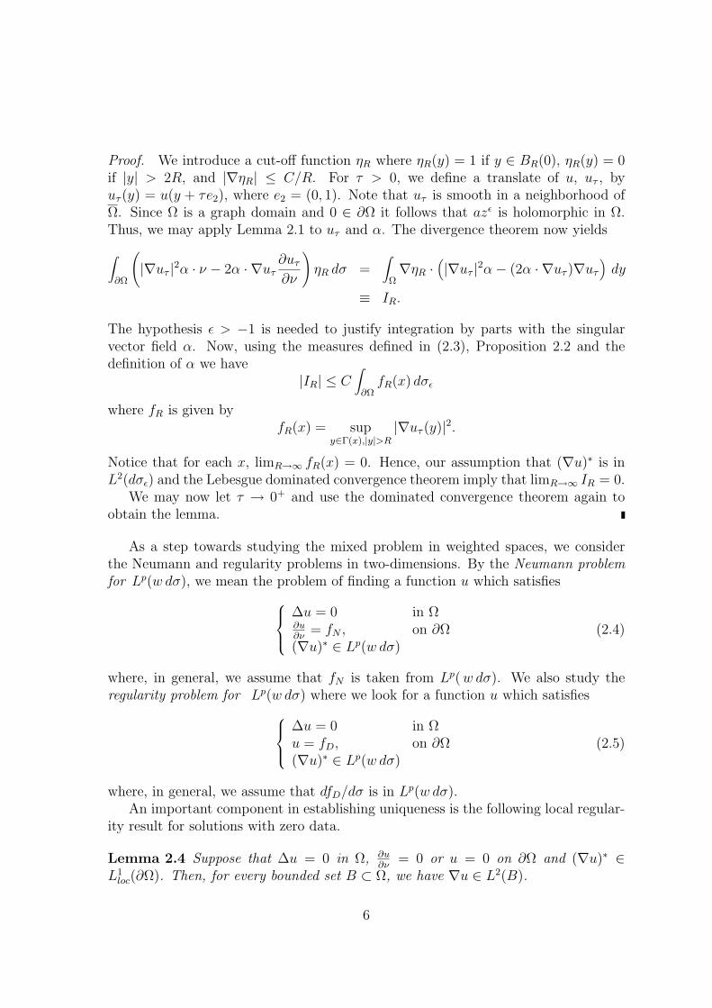
Proof. We introduce a cut-off function ηR where ηR(y) = 1 if y ∈ BR(0), ηR(y) = 0if |y| > 2R, and |∇ηR| ≤ C/R. For τ > 0, we define a translate of u, uτ , byuτ (y) = u(y + τe2), where e2 = (0, 1). Note that uτ is smooth in a neighborhood ofΩ. Since Ω is a graph domain and 0 ∈ ∂Ω it follows that azε is holomorphic in Ω.Thus, we may apply Lemma 2.1 to uτ and α. The divergence theorem now yields

∫∂Ω

(|∇uτ |2α · ν − 2α · ∇uτ

∂uτ∂ν

)ηR dσ =

∫Ω∇ηR ·

(|∇uτ |2α− (2α · ∇uτ )∇uτ

)dy

≡ IR.

The hypothesis ε > −1 is needed to justify integration by parts with the singularvector field α. Now, using the measures defined in (2.3), Proposition 2.2 and thedefinition of α we have

|IR| ≤ C∫∂ΩfR(x) dσε

where fR is given byfR(x) = sup

y∈Γ(x),|y|>R|∇uτ (y)|2.

Notice that for each x, limR→∞ fR(x) = 0. Hence, our assumption that (∇u)∗ is inL2(dσε) and the Lebesgue dominated convergence theorem imply that limR→∞ IR = 0.

We may now let τ → 0+ and use the dominated convergence theorem again toobtain the lemma.

As a step towards studying the mixed problem in weighted spaces, we considerthe Neumann and regularity problems in two-dimensions. By the Neumann problemfor Lp(w dσ), we mean the problem of finding a function u which satisfies

∆u = 0 in Ω∂u∂ν

= fN , on ∂Ω(∇u)∗ ∈ Lp(w dσ)

(2.4)

where, in general, we assume that fN is taken from Lp(w dσ). We also study theregularity problem for Lp(w dσ) where we look for a function u which satisfies

∆u = 0 in Ωu = fD, on ∂Ω(∇u)∗ ∈ Lp(w dσ)

(2.5)

where, in general, we assume that dfD/dσ is in Lp(w dσ).An important component in establishing uniqueness is the following local regular-

ity result for solutions with zero data.

Lemma 2.4 Suppose that ∆u = 0 in Ω, ∂u∂ν

= 0 or u = 0 on ∂Ω and (∇u)∗ ∈L1loc(∂Ω). Then, for every bounded set B ⊂ Ω, we have ∇u ∈ L2(B).

6

Proof. We consider the case of Neumann boundary conditions. Dirichlet boundaryconditions may be handled by a similar argument.

We first observe that since (∇u)∗ is in L1loc(dσ), it follows that ∇u is in L1(B) for

any bounded subset of Ω, B.Fix a point x0 ∈ ∂Ω and let η be a smooth cutoff function which is one on B2r(x0)

and zero outside of B4r(x0). We let N(z, y) be the Neumann function for Ω, thus N isa fundamental solution which satisfies homogeneous Neumann boundary conditions.Dahlberg and Kenig [10] construct the Neumann function on a graph domain byreflection. At least formally, we have the representation formula,

ηu(z) =∫Ω∩B4r(x0)

N(z, y)(u(y)∆η(y) + 2∇u(y) · ∇η(y)) dy (2.6)

−∫∆4r(x0)

N(z, t)u(t)∂η(t)

∂νdσ(t) , z ∈ Ω.

We now show how to estimate each term on the right-hand side of this formula.Since (∇u)∗(x) is in L1

loc(∂Ω), it follows that u is bounded on ∆4r(x0). As we observedabove, we have ∇u ∈ L1(Ω ∩B4r(x0)), and the Poincare inequality gives that u is inL1(Ω ∩ B3r(x0)). We also have that the Neumann function is locally bounded whenz 6= y. Hence, the integrands in (2.6) are in L1 and it is a routine matter to justifythis formula. Since the map y → N(z, y) is in the Sobolev space W 1,2(Br(x0) ∩ Ω),uniformly for z ∈ B3r(x0) \ B2r(x0), the estimates for u and ∇u outlined abovetogether with (2.6) imply that ∇u ∈ L2(Br(x0) ∩ Ω).

Next, we recall a classical fact from harmonic function theory, a Phragmen-Lindelof theorem. This result is well-known and may be found in Protter and Wein-berger [28, Section 9, Theorem 18]. We will need this theorem to control the behaviorat infinity of solutions in our unbounded domains.

In the next result and below, we will let Ωϕ denote the sector

Ωϕ = reiθ : r > 0, |θ − π/2| < ϕ, 0 < ϕ < π . (2.7)

With this normalization, Ωϕ is a Lipschitz domain with constant M = | tan(π/2−ϕ)|.

Theorem 2.5 (Phragmen-Lindelof) Let ϕ ∈ (0, π). Suppose v is sub-harmonicin Ωϕ, v = 0 on ∂Ωϕ and

v(z) = o(|z|π/(2ϕ)) as |z| → +∞ , z ∈ Ωϕ .

Then v ≤ 0.

We now prove uniqueness for the regularity problem for Lp(w dσ), (2.5).

7

Lemma 2.6 Let Ω be a Lipschitz graph domain with Lipschitz constant M . Supposethat, for p ≥ 1, Lploc(w dσ) ⊂ L1

loc(dσ) and that that for all surface balls ∆r(x) withr > 1, we have

(∫∆r(x)

w(t)−1/(p−1) dσ(t)

) p−1p

≤ Crπ/(2β+π), if p > 1; (2.8)(inf

t∈∆r(x)w(t)

)−1

≤ Crπ/(2β+π), if p = 1 (2.9)

where β = arctanM > 0. Under these conditions, if u is harmonic in Ω, (∇u)∗ ∈Lp(w dσ) and u = 0 on ∂Ω, then u = 0 in Ω.

Proof. Since β = arctanM then we have Ω ⊂ Ωϕ, with ϕ = β + π/2. Define v by

v(x) =

|u|, in Ω0, in Ωc.

The function v is sub-harmonic in all of R2 and, moreover, v = 0 on ∂Ωϕ. We verifythe growth condition in the Phragmen-Lindelof Theorem 2.5. To do this, supposethat z ∈ Ωϕ and set r = |z|. By Lemma 2.4 we have that ∇u is in L2 of eachbounded subset of Ω, and the same is true for ∇v. Then, by combining the mean-value property for sub-harmonic functions with the Poincare inequality, Proposition2.2 (for the Carleson measure dµ(y) = 1

rχBr(z) dy with respect to dσ, see (2.3)) and

Holder’s inequality, in the case p > 1, we obtain

0 ≤ v(z) ≤ 1

πr2

∫Br(z)

v(y) dy

≤ C

r

∫Br(z)

|∇v(y)| dy

≤ C∫∆2r(x)

(∇u)∗(t) dσ(t)

≤ C

(∫∆2r(x)

(∇u)∗(t)pw(t)dσ(t)

)1/p (∫∆2r(x)

w−1/(p−1)(t) dσ(t)

) p−1p

.

Here, x is the projection of z onto the boundary, i.e. if z = (x1, φ(x1) + t), thenx = (x1, φ(x1)). Thus, under our assumption (2.8) it follows that

0 ≤ v(z) ≤ Crπ2ϕ ≤ C|z|

π2ϕ , z ∈ Ωϕ ,

as 0 ∈ ∂Ωϕ. We may now apply Phragmen-Lindelof Theorem 2.5 and conclude thatv = 0. The case p = 1 is treated in a similar fashion.

8

Remark. Using Holder’s inequality, we see that

∫∆s(x)

|f(t)| dσ(t) ≤(∫

∆s(x)|f(t)|pw(t) dσ(t)

)1/p (∫∆s(x)

w(t)−1/(p−1) dσ(t)

) p−1p

.

Thus, we have Lploc(w dσ) ⊂ L1loc(dσ) provided w−1/(p−1) is in L1

loc(dσ). It is easy tosee that this will hold for the weight w(t) = |t|ε if ε < p− 1.

Finally, we give uniqueness for the weighted Neumann problem for Lp(w dσ), (2.4).

Lemma 2.7 Let Ω be a Lipschitz graph domain with Lipschitz constant M . Supposew satisfies the hypotheses of Lemma 2.6. If u is a solution of the Neumann problemwith (∇u)∗ ∈ Lp(w dσ), p ≥ 1, and ∂u

∂ν= 0 a.e. ∂Ω, then u is constant.

Proof. We consider v, the conjugate harmonic function to u. Since u has normalderivative zero at the boundary, by the Cauchy-Riemann equations we have that vis constant on the boundary, and we may assume this constant is 0. Now, (∇v)∗ ∈Lp(w dσ) (since this is the case for u) so that v satisfies the hypotheses of Lemma 2.6and hence it is zero. But this implies that u is constant.

3 The L2-Neumann and regularity problems with

power weights

In this section we outline the proof of existence of solutions to the Neumann problemand the regularity problem for L2(w dσ) when the weight is a power of |x|. Theseresults are due to Shen [30, Theorems 1.7, 1.9]. Shen’s results are stated for boundeddomains in three dimensions. We give a few steps of the proof to indicate the minormodifications that are needed to handle graph domains in two dimensions.

Before continuing, we record a few basic facts about the power weights |x|ε andtheir relation to the Muckenhoupt class Ap(dσ). A weight (that is a non-negativemeasurable and locally integrable function) w is a member of the class Ap(dσ) if andonly if for all surface balls ∆ ⊂ ∂Ω, we have

1

σ(∆)

∫∆w dσ

(1

σ(∆)

∫∆w

−1p−1 dσ

)p−1

≤ C.

The best constant C in this inequality is called the Ap-constant for w. The followingsimple lemma tells us that |x|ε is in Ap(dσ) if and only if −1 < ε < p − 1, see [31,p. 218].

Lemma 3.1 For ε > −1, the boundary measure σε (see (2.3)) satisfies

σε(∆r(x)) ≈ rmax(|x|, r)ε, x ∈ ∂Ω.

9

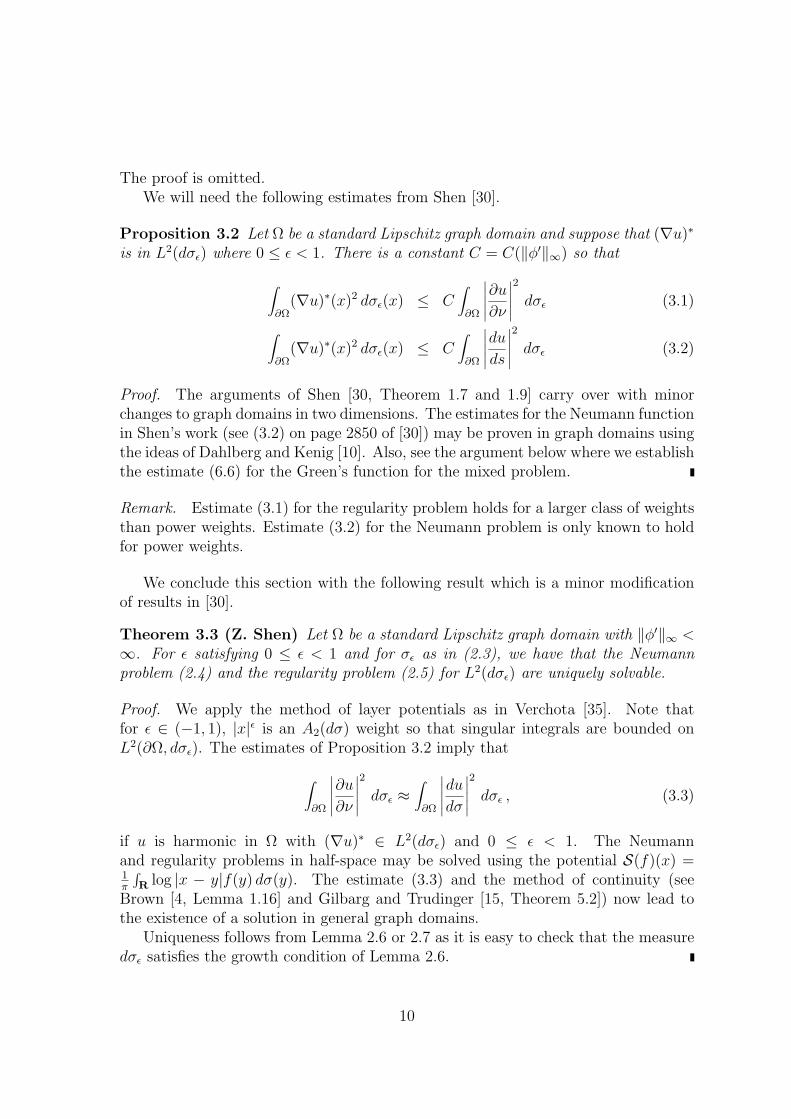
The proof is omitted.We will need the following estimates from Shen [30].

Proposition 3.2 Let Ω be a standard Lipschitz graph domain and suppose that (∇u)∗is in L2(dσε) where 0 ≤ ε < 1. There is a constant C = C(‖φ′‖∞) so that

∫∂Ω

(∇u)∗(x)2 dσε(x) ≤ C∫∂Ω

∣∣∣∣∣∂u∂ν∣∣∣∣∣2

dσε (3.1)

∫∂Ω

(∇u)∗(x)2 dσε(x) ≤ C∫∂Ω

∣∣∣∣∣duds∣∣∣∣∣2

dσε (3.2)

Proof. The arguments of Shen [30, Theorem 1.7 and 1.9] carry over with minorchanges to graph domains in two dimensions. The estimates for the Neumann functionin Shen’s work (see (3.2) on page 2850 of [30]) may be proven in graph domains usingthe ideas of Dahlberg and Kenig [10]. Also, see the argument below where we establishthe estimate (6.6) for the Green’s function for the mixed problem.

Remark. Estimate (3.1) for the regularity problem holds for a larger class of weightsthan power weights. Estimate (3.2) for the Neumann problem is only known to holdfor power weights.

We conclude this section with the following result which is a minor modificationof results in [30].

Theorem 3.3 (Z. Shen) Let Ω be a standard Lipschitz graph domain with ‖φ′‖∞ <∞. For ε satisfying 0 ≤ ε < 1 and for σε as in (2.3), we have that the Neumannproblem (2.4) and the regularity problem (2.5) for L2(dσε) are uniquely solvable.

Proof. We apply the method of layer potentials as in Verchota [35]. Note thatfor ε ∈ (−1, 1), |x|ε is an A2(dσ) weight so that singular integrals are bounded onL2(∂Ω, dσε). The estimates of Proposition 3.2 imply that

∫∂Ω

∣∣∣∣∣∂u∂ν∣∣∣∣∣2

dσε ≈∫∂Ω

∣∣∣∣∣dudσ∣∣∣∣∣2

dσε , (3.3)

if u is harmonic in Ω with (∇u)∗ ∈ L2(dσε) and 0 ≤ ε < 1. The Neumannand regularity problems in half-space may be solved using the potential S(f)(x) =1π

∫R log |x − y|f(y) dσ(y). The estimate (3.3) and the method of continuity (see

Brown [4, Lemma 1.16] and Gilbarg and Trudinger [15, Theorem 5.2]) now lead tothe existence of a solution in general graph domains.

Uniqueness follows from Lemma 2.6 or 2.7 as it is easy to check that the measuredσε satisfies the growth condition of Lemma 2.6.

10

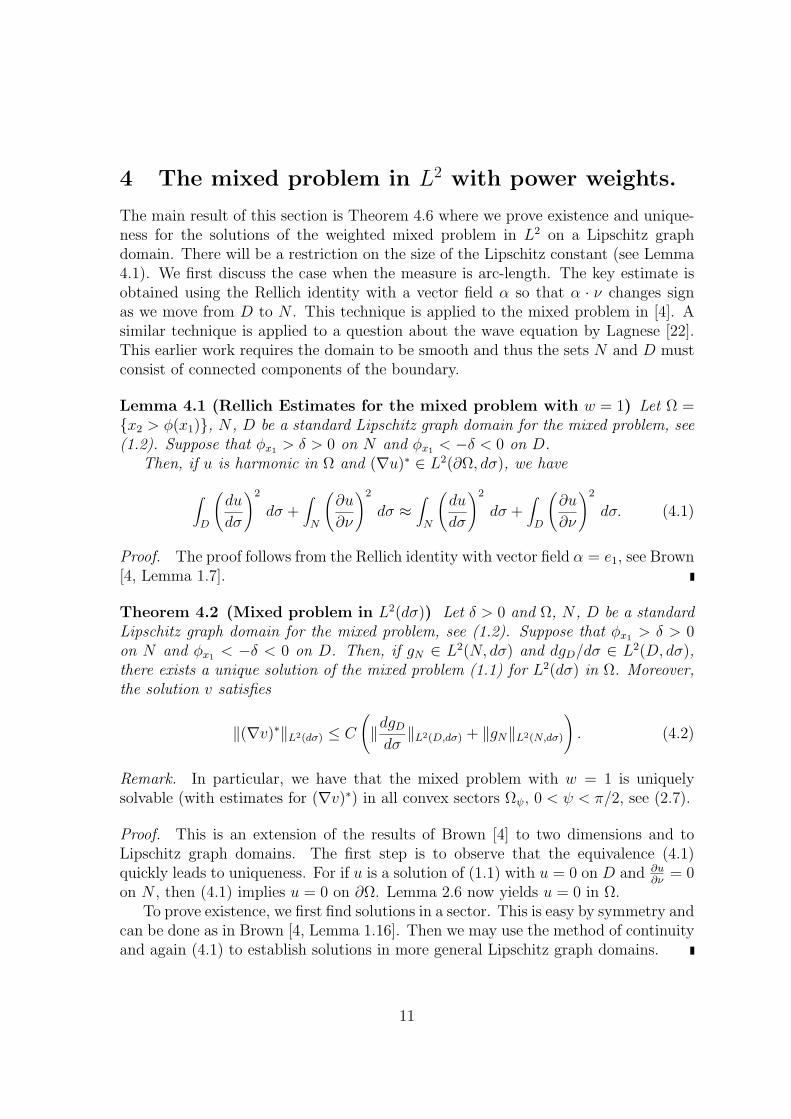
4 The mixed problem in L2 with power weights.

The main result of this section is Theorem 4.6 where we prove existence and unique-ness for the solutions of the weighted mixed problem in L2 on a Lipschitz graphdomain. There will be a restriction on the size of the Lipschitz constant (see Lemma4.1). We first discuss the case when the measure is arc-length. The key estimate isobtained using the Rellich identity with a vector field α so that α · ν changes signas we move from D to N . This technique is applied to the mixed problem in [4]. Asimilar technique is applied to a question about the wave equation by Lagnese [22].This earlier work requires the domain to be smooth and thus the sets N and D mustconsist of connected components of the boundary.

Lemma 4.1 (Rellich Estimates for the mixed problem with w = 1) Let Ω =x2 > φ(x1), N , D be a standard Lipschitz graph domain for the mixed problem, see(1.2). Suppose that φx1 > δ > 0 on N and φx1 < −δ < 0 on D.

Then, if u is harmonic in Ω and (∇u)∗ ∈ L2(∂Ω, dσ), we have

∫D

(du

dσ

)2

dσ +∫N

(∂u

∂ν

)2

dσ ≈∫N

(du

dσ

)2

dσ +∫D

(∂u

∂ν

)2

dσ. (4.1)

Proof. The proof follows from the Rellich identity with vector field α = e1, see Brown[4, Lemma 1.7].

Theorem 4.2 (Mixed problem in L2(dσ)) Let δ > 0 and Ω, N , D be a standardLipschitz graph domain for the mixed problem, see (1.2). Suppose that φx1 > δ > 0on N and φx1 < −δ < 0 on D. Then, if gN ∈ L2(N, dσ) and dgD/dσ ∈ L2(D, dσ),there exists a unique solution of the mixed problem (1.1) for L2(dσ) in Ω. Moreover,the solution v satisfies

‖(∇v)∗‖L2(dσ) ≤ C

(‖dgDdσ

‖L2(D,dσ) + ‖gN‖L2(N,dσ)

). (4.2)

Remark. In particular, we have that the mixed problem with w = 1 is uniquelysolvable (with estimates for (∇v)∗) in all convex sectors Ωψ, 0 < ψ < π/2, see (2.7).

Proof. This is an extension of the results of Brown [4] to two dimensions and toLipschitz graph domains. The first step is to observe that the equivalence (4.1)quickly leads to uniqueness. For if u is a solution of (1.1) with u = 0 on D and ∂u

∂ν= 0

on N , then (4.1) implies u = 0 on ∂Ω. Lemma 2.6 now yields u = 0 in Ω.To prove existence, we first find solutions in a sector. This is easy by symmetry and

can be done as in Brown [4, Lemma 1.16]. Then we may use the method of continuityand again (4.1) to establish solutions in more general Lipschitz graph domains.

11

We now turn our attention to the weighted mixed problem in sectors that are notconvex. For the boundary of a sector Ωϕ as in (2.7), we write: ∂Ωϕ = Dϕ ∪Nϕ, withD and N as in (1.2).

Proposition 4.3 (Weighted mixed problem on sectors) Let ϕ ∈ (π/2, π) andsuppose that 1 − π

2ϕ< ε < 1. Let σε be as in (2.3). Then, if fN ∈ L2(Nϕ, dσε) and

dfD/dσ ∈ L2(Dϕ, dσε), there exists a unique solution u of the mixed problem∆u = 0 in Ωϕ

u = fD on Dϕ∂u∂ν

= fN on Nϕ

(∇u)∗ ∈ L2(∂Ωϕ, dσε).

(4.3)

Moreover, u satisfies

∫∂Ωϕ

(∇u)∗(x)2 dσε ≤ C

∫Nϕ

|fN(x)|2 dσε +∫Dϕ

∣∣∣∣∣dfDdσ (x)

∣∣∣∣∣2

dσε

(4.4)

Proof. We use a conformal map to reduce the weighted mixed problem (4.3) to themixed problem with weight w = 1 on a convex sector, then we apply Theorem 4.2.

Let s = 1− ε with ε as in the hypothesis, so that we have

0 < s < π/2ϕ < 1. (4.5)

Define hs(z) to be the conformal map

η = hs(z) = i(−iz)s.

Thus, hs maps Ωϕ to Ωsϕ, Dϕ to Dsϕ and Nϕ to Nsϕ. Note that if we let ∂hs denotethe complex derivative of hs, that is

∂hs =1

2

(∂hs∂x1

+1

i

∂hs∂x2

)(4.6)

we have1

|∂hs|dσ =

1

sdσε . (4.7)

On account of (4.5) it follows that Ωsϕ is a convex sector and thus Theorem 4.2 appliesto Ωsϕ.

Given fD and fN as in (4.3), we define gD and gN on ∂Ωsϕ as follows:

gN(η) =fN|∂hs|

h−1s (η) ; gD(η) = fD h−1

s (η).

12

We verify that gN and gD satisfy the hypotheses of Theorem 4.2. Indeed, it is imme-diate to see that ∫

Nsϕ

|gN |2dσ =1

s

∫Nϕ

|fN |2dσε . (4.8)

Similarly, we have ∫Nsϕ

∣∣∣∣∣dgDdσ∣∣∣∣∣2

dσ =1

s

∫Nϕ

∣∣∣∣∣dfDdσ∣∣∣∣∣2

dσε . (4.9)

By Theorem 4.2 the mixed problem in L2(dσ) on Ωsϕ has a unique solution vwhich satisfies (4.2). We now pull this solution back to Ωϕ by defining u = v hs.Then, u is harmonic in Ωϕ and satisfies:

u = fD on Dϕ ;∂u

∂ν= fN on Nϕ .

Moreover, on account of (4.2), (4.8) and (4.9) we have

‖(∇v)∗‖L2(∂Ωsϕ ,dσ) ≤ C∫Nϕ

|fN(x)|2 dσε +∫Dϕ

∣∣∣∣∣dfDds (x)

∣∣∣∣∣2

dσε. (4.10)

Now we consider non-tangential maximal function estimates for ∇u. We applythe Cauchy integral formula to the complex derivative of u (which is analytic in Ωϕ)and obtain:

∂u(z) =1

2πi

∫∂Ωϕ

∂u(ζ)

z − ζdζ =

1

2πi

∫∂Ωϕ

∂hs(ζ)∂v(hs(ζ))

z − ζdζ , z ∈ Ωϕ .

It follows

(∇u)∗(x) = 2(∂u)∗(x) ≤(Kϕ(∂hs · (∂v) hs)

)∗(x) , a.e. x ∈ ∂Ωϕ ,

where Kϕ denotes the Cauchy integral on Ωϕ. By the theorem of Coifman, McIntoshand Meyer [7] on the boundedness of the Cauchy integral we have

‖(Kϕψ)∗‖L2(∂Ωϕ,dσε) ≤ C‖ψ‖L2(∂Ωϕ,dσε).

This uses that dσε is in A2(dσ). Combining these last two inequalities we obtain

‖(∇u)∗‖L2(∂Ωϕ,dσε) ≤ C‖∂hs · (∂v) hs)‖L2(∂Ωϕ,dσε) = C‖∂v‖L2(∂Ωsϕ,dσ) , (4.11)

where the last equality was obtained by performing the change of variables hs(ζ) = η,see also (4.7). This, together with (4.10) yields (4.4).

The argument is reversible, so we may conclude uniqueness in Ωϕ from uniquenessin Ωsϕ.

13

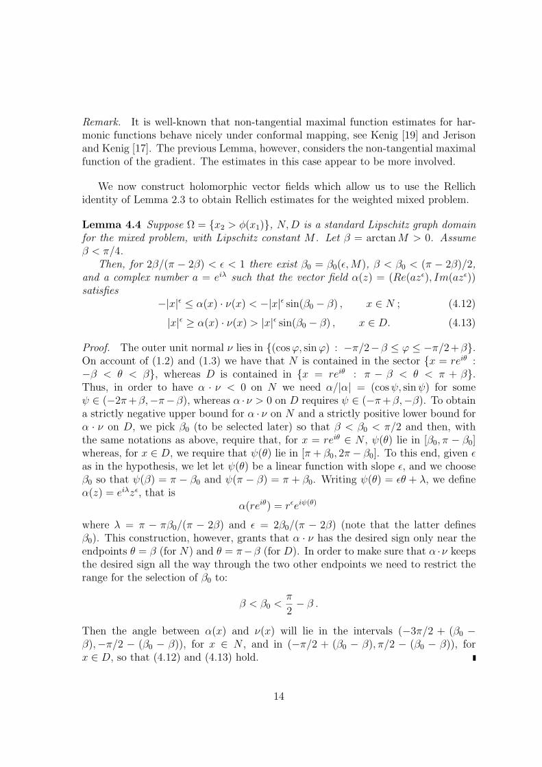
Remark. It is well-known that non-tangential maximal function estimates for har-monic functions behave nicely under conformal mapping, see Kenig [19] and Jerisonand Kenig [17]. The previous Lemma, however, considers the non-tangential maximalfunction of the gradient. The estimates in this case appear to be more involved.

We now construct holomorphic vector fields which allow us to use the Rellichidentity of Lemma 2.3 to obtain Rellich estimates for the weighted mixed problem.

Lemma 4.4 Suppose Ω = x2 > φ(x1), N,D is a standard Lipschitz graph domainfor the mixed problem, with Lipschitz constant M . Let β = arctanM > 0. Assumeβ < π/4.

Then, for 2β/(π − 2β) < ε < 1 there exist β0 = β0(ε,M), β < β0 < (π − 2β)/2,and a complex number a = eiλ such that the vector field α(z) = (Re(azε), Im(azε))satisfies

−|x|ε ≤ α(x) · ν(x) < −|x|ε sin(β0 − β) , x ∈ N ; (4.12)

|x|ε ≥ α(x) · ν(x) > |x|ε sin(β0 − β) , x ∈ D. (4.13)

Proof. The outer unit normal ν lies in (cosϕ, sinϕ) : −π/2−β ≤ ϕ ≤ −π/2+β.On account of (1.2) and (1.3) we have that N is contained in the sector x = reiθ :−β < θ < β, whereas D is contained in x = reiθ : π − β < θ < π + β.Thus, in order to have α · ν < 0 on N we need α/|α| = (cosψ, sinψ) for someψ ∈ (−2π+β,−π−β), whereas α ·ν > 0 on D requires ψ ∈ (−π+β,−β). To obtaina strictly negative upper bound for α · ν on N and a strictly positive lower bound forα · ν on D, we pick β0 (to be selected later) so that β < β0 < π/2 and then, withthe same notations as above, require that, for x = reiθ ∈ N , ψ(θ) lie in [β0, π − β0]whereas, for x ∈ D, we require that ψ(θ) lie in [π + β0, 2π − β0]. To this end, given εas in the hypothesis, we let let ψ(θ) be a linear function with slope ε, and we chooseβ0 so that ψ(β) = π − β0 and ψ(π − β) = π + β0. Writing ψ(θ) = εθ + λ, we defineα(z) = eiλzε, that is

α(reiθ) = rεeiψ(θ)

where λ = π − πβ0/(π − 2β) and ε = 2β0/(π − 2β) (note that the latter definesβ0). This construction, however, grants that α · ν has the desired sign only near theendpoints θ = β (for N) and θ = π−β (for D). In order to make sure that α ·ν keepsthe desired sign all the way through the two other endpoints we need to restrict therange for the selection of β0 to:

β < β0 <π

2− β .

Then the angle between α(x) and ν(x) will lie in the intervals (−3π/2 + (β0 −β),−π/2 − (β0 − β)), for x ∈ N , and in (−π/2 + (β0 − β), π/2 − (β0 − β)), forx ∈ D, so that (4.12) and (4.13) hold.

14

Proposition 4.5 (Weighted Rellich estimates for the mixed problem) Let Ω,N , D be a standard Lipschitz graph domain for the mixed problem (1.1), with Lips-chitz constant M < 1. Let β = arctanM . Then, for σε as in (2.3), for ε in the range2β/(π − 2β) < ε < 1 and for u harmonic with (∇u)∗ ∈ L2(dσε), we have∫

∂Ω(∇u)∗(x)2 dσε ≤ C

∫N

(∂u

∂ν

)2

dσε +∫D

(du

dσ

)2

dσε

.Proof. The identity of Lemma 2.3 together with the vector field constructed inLemma 4.4 and standard manipulations involving the boundary terms as in Brown[4, Lemma 1.7] yield the estimate∫

∂Ω|∇u|(x)2 dσε ≤ C

∫N

(∂u

∂ν

)2

dσε +∫D

(du

dσ

)2

dσε

.The key point is that since α ·ν changes sign as we pass from N to D, we can estimatethe full gradient of u on the boundary by the data for the mixed problem.

In order to obtain the estimate for the non-tangential maximal function of ∇u,we argue as in Proposition 4.3. We may represent the holomorphic function ∂u usingthe Cauchy kernel

∂u(x) =1

2πi

∫∂Ω

∂u(y)

x− ydy. (4.14)

Since σε is an A2 weight with respect to σ for −1 < ε < 1, the theorem of Coifman,McIntosh and Meyer [7] implies the non-tangential maximal estimate ‖(∂u)∗‖L2(σε) ≤C‖∂u‖L2(σε). The estimate of the proposition follows from this and the correspondingestimate for ∂u.

Theorem 4.6 (Mixed problem in L2(σε)) Suppose Ω, N and D is a standardLipschitz graph domain for the mixed problem with Lipschitz constant M < 1. Letβ = arctan(M). Given ε which satisfies

2β/(π − 2β) < ε < 1,

there is a unique solution u to the L2(dσε) mixed problem (1.1). Moreover, u satisfies∫∂Ω

(∇u)∗(x)2 dσε ≤

∫D

∣∣∣∣∣dfDdσ∣∣∣∣∣2

dσε +∫N|fN |2 dσε

.Proof. Using the estimate of Proposition 4.5, the existence result for sectors inProposition 4.3, and the method of continuity (see Brown [4, Lemma 1.16] and Gilbargand Trudinger [15, Theorem 5.2]), we obtain the existence of a solution to the mixedproblem with data in L2(dσε).

Next, we consider uniqueness. If u is a solution of the mixed problem with zerodata, then the Rellich estimates or Proposition 4.5 imply that u is a solution ofthe regularity and Neumann problems for L2(dσε) with zero data. By the results inSection 2 it follows that u is zero.

15

5 The regularity and Neumann problems in H1(dσε).

In this section we assert the existence of solutions for the Neumann problem when thedata is in H1(dσε), and for the regularity problem when the data has one derivativein H1(dσε). The proof of these results follows the work of Dahlberg and Kenig [10];thus, we shall be brief. We first recall the definition of the Hardy spaces H1(dσε) andH1,1(dσε).

Let ε > −1. We say that a is an H1(dσε)-atom for ∂Ω if a is supported on asurface ball ∆s(x),

∫a dσ = 0 and ‖a‖∞ ≤ [σε(∆s(x))]

−1. We remark that for ε ≤ 0,L1(dσε) ⊂ L1

loc(dσ). Thus we define the space H1(dσε), for ε ≤ 0, to be the collectionof functions that are represented as

f(x) =∞∑j=1

λjaj(x) (5.1)

where ajj∈N is a sequence of H1(dσε)-atoms for ∂Ω and the coefficients λj satisfy∑∞j=1 |λj| < ∞. The sum for f in (5.1) converges in L1(dσε). the sum converges in

L1(dσε). The H1(dσε)-norm is defined by

‖f‖H1(dσε) = inf∑

|λj| (5.2)

where the infimum is taken over all possible representations of f . Note that whileH1(dσε)-atoms are defined for ε > −1, we consider (and need for our application inTheorem 7.2) the space H1(dσε) only for ε ≤ 0. This allows us to avoid having todefine spaces of distributions on Lipschitz graph domains. (See Coifman and Weiss[8] or Stromberg and Torchinsky [32] for a discussion of these spaces.)

Let ε ≤ 0. We say that A is an H1,1(dσε)-atom for ∂Ω if for some x0 in ∂Ω

A(x) =∫ x

x0

a(t)dσ(t), x ∈ ∂Ω

where a is an H1(dσε)-atom, and∫ xx0

denotes integration along the portion of theboundary ∂Ω with endpoints x0 and x. Given an H1(dσε)-atom a, the integral abovedefines A uniquely up to an additive constant. For ε ≤ 0, we define the spaceH1,1(dσε)to be sums of the form

F (x) =∞∑j=1

λjAj(x)

where the coefficients satisfy∑∞j=1 |λj| <∞. The norm of F in H1,1(σε′), ‖F‖H1,1(dσε),

is defined to be the infimum of∑∞j=1 |λj| over all possible representations of F as sums

of atoms. If we choose the base point x0 for each atom to be zero, then we have thatthe sum defining F converges in the norm given by

sup |x|−ε|F (x)|.

16

Furthermore, it is easy to see that we have

‖F‖H1,1(dσε) = ‖dFdσ‖H1(dσε).

By the Neumann problem for H1(dσε) we mean the Neumann problem for L1(dσε),see (2.4), where the data fN is now taken from H1(dσε). By the regularity problemfor H1,1(dσε) we mean the regularity problem for L1(dσε), see (2.5), where the datafD is taken from H1,1(dσε).

For future reference, we also define spaces on subsets of the boundary. A functionf is in H1(N, dσε) if and only if f is the restriction to N of a function in H1(dσε).Such functions can be written as sums of atoms that are restrictions to N of H1(dσε)-atoms for ∂Ω. The space H1,1(D, dσε) is defined in a similar fashion. See Chang,Krantz and Stein [6], Sykes [33], and Sykes and Brown [34] for additional works thatstudy Hardy spaces on domains.

The main result of this section is the following theorem. We omit the proof sinceit is quite similar to the argument for the mixed problem in the following section(Theorem 7.2).

Theorem 5.1 Let Ω be a standard Lipschitz graph domain with Lipschitz constantM and let ε0(M) < ε′ ≤ 0 be small. Then the H1(dσε′)-Neumann and the H1,1(dσε′)-regularity problems are uniquely solvable. The solutions satisfy, respectively,

‖u‖H1,1(dσε′ )+∫∂Ω

(∇u)∗(x) dσε′ ≤ C

∥∥∥∥∥∂u∂ν∥∥∥∥∥H1(dσε′ )∥∥∥∥∥∂u∂ν

∥∥∥∥∥H1(dσε′ )

+∫∂Ω

(∇u)∗(x) dσε′ ≤ C‖u‖H1,1(dσε′ ).

Remark. We do not assert uniqueness when ε′ > 0. In the rest of this paper, we willonly use the existence of a solution for the H1(dσε′)-Neumann problem in the casewhen ε′ ≤ 0. (In order to fully treat the case ε′ > 0, one needs to give a differentdefinition of the normal derivative at the boundary. For ε′ > 0 the H1(dσε′)-boundarydata may not be in L1

loc(dσ) and hence fail to be a function. See Brown [5] and Fabes,Mendez and Mitrea [13] for a treatment of the Neumann problem with data which isnot locally integrable).

6 The mixed problem in H1 with power weights.

By the mixed problem for H1(dσε′) we mean the mixed problem for L1(dσε′), see (1.1),where the Dirichlet data fD is taken from H1,1(D, dσε′) and the Neumann data fN isin H1(N, dσε′). In this section, we consider the mixed problem where the Neumanndata is an H1(N, dσε′) atom and the Dirichlet data is zero. Since atoms lie in L2(dσε)

17

for ε > −1, Theorem 4.6 yields existence and uniqueness of the solution to the mixedproblem for L2(dσε) with these data. Our first goal is to show that the gradient ofthe solution also has non-tangential maximal function in L1(dσε′), for ε′ near zero.

Theorem 6.1 Suppose Ω, N , D is a standard Lipschitz graph domain for the mixedproblem with Lipschitz constant M < 1 and set β = tan−1M . Then, there is δ =δ(M) with 1 > δ > 0 so that, for ε′ satisfying 4β−π

2(π−2β)< ε′ < δ we may solve the

mixed problem (1.1) for H1(dσε′) with zero Dirichlet data and with Neumann data anH1(N, dσε′)-atom, a. The solution u satisfies the estimate∫

∂Ω(∇u)∗(x) dσε′ ≤ C(M, ε′) . (6.1)

In addition, we have

‖u‖H1,1(dσε′ )+

∥∥∥∥∥∂u∂ν∥∥∥∥∥H1(dσε′ )

≤ C(M, ε′). (6.2)

As a step towards the proof of Theorem 6.1, we construct a Green’s functionfor the mixed problem using the method of reflections–an old idea that was used byDahlberg and Kenig [10] to obtain a similar result for the Neumann and regularityproblems. The estimates for the Green’s function are a consequence of the Holderregularity of weak solutions of divergence-form equations with bounded measurablecoefficients.

We begin by constructing a bi-Lipschitz map, Φ : R2 → R2 with Φ(Ω) = Qwhere Q is the first quadrant, Q = (x1, x2) : x1 > 0, x2 > 0. We also require thatΦ(N) = (x1, x2) : x1 ≥ 0, x2 = 0 and Φ(D) = (x1, x2) : x1 = 0, x2 > 0. On Qwe now define the operator L = divA∇ where the coefficient matrix A has boundedentries (these are first-order derivatives of Φ), so that u satisfies

∆u = 0, in Ω∂u∂ν

= fN , on Nu = fD, on D

if and only if the function v defined by v = u Φ−1 satisfiesLv = 0, in QA∇v · ν = fN Φ−1 on Φ(N)v = fD Φ−1 on Φ(D)

Now, we extend the coefficients of L by reflection, so that Lv = 0 if and only if L(v Rj) = 0 where R1 and R2 are the reflections R1(x1, x2) = (−x1, x2) and R2(x1, x2) =(x1,−x2). Next, letting G denote the Green’s function for L in Q, we set

N (z, w) = G(z, w)−G(z, R1w) +G(z, R2w)−G(z, R1R2w) , z, w ∈ Q

18

and observe that N is a Green’s function for the mixed problem for L in Q. Recallthat we may find a Green’s function for L in Q which satisfies

|G(z, w)| ≤ C(1 + | log |z − w||) , z, w ∈ Q,

see Kenig and Ni [21]. We then observe that if |z − ζ| = 1 and |ζ − w| < 1/2, then|G(z, ζ)−G(z, w)| ≤ C|ζ −w|δ, where 0 < δ < 1, δ = δ(M). This is a standard esti-mate of Holder continuity for solutions of divergence-form elliptic operators. Finally,by rescaling, we obtain

|G(z, ζ)−G(z, w)| ≤ C

(|ζ − w||z − ζ|

)δ, if |ζ − w| < 1

2|z − ζ|. (6.3)

The latter immediately implies the same estimate for N in Q, namely

|N (z, ζ)−N (z, w)| ≤ C

(|ζ − w||z − ζ|

)δif z, ζ, w ∈ Q and |ζ − w| < 1

2|z − ζ| (6.4)

We will need an additional estimate for N (z, ζ) when ζ ∈ Q is near Φ(D). Sincewe have N (z, x) = 0 if z ∈ Q and x ∈ Φ(D), it follows by continuity that N is smallnear Φ(D). More precisely, let ζ ∈ Q and suppose that x is a point on Φ(D) forwhich |x− ζ| = dist(ζ,Φ(D)). For z ∈ Q, we have N (z, x) = 0 and (6.4) implies

|N (z, ζ)| ≤ C|ζ|δ

|z − ζ|δ, if z, ζ ∈ Q and dist(ζ,D) <

1

2|z − ζ|, (6.5)

(here we have used that 0 ∈ ∂Q). Finally, we define the Green’s function for themixed problem by

M(x, y) = N (Φ(x),Φ(y)).

Since Φ is bi-Lipschitz the estimates (6.4) and (6.5) imply similar results for M in Ω:

|M(x, ζ)−M(z, w)| ≤ C

(|ζ − w||z − ζ|

)δ,

if z, ζ, w ∈ Ω with |ζ − w| < 1

2|z − ζ| (6.6)

|M(z, ζ)| ≤ C|ζ|δ

|z − ζ|δ

ifz, ζ ∈ Ω and dist(ζ,D) <1

2|z − ζ|. (6.7)

These estimates are a key ingredient in the study of the behavior of the solutionof the mixed problem with atomic Neumann data.

19

Lemma 6.2 Assume ε′ > −1. Let u be a solution of the mixed problem (1.1) forL1(dσε′), where the Neumann data is an H1(N, dσε′)-atom, a, and the Dirichlet datais zero. Then, for any integer k ≥ 1, u satisfies

|u(z)| ≤ Cρδ

|z − xa|δσ(∆ρ(xa))

σε′(∆ρ(xa)), z ∈ Ω , |z − xa| ≥ 2kρ.

Here, 0 < δ < 1 is as in the estimate for the Green’s function for the mixed problem(6.3) and ∆ρ(xa) is the surface ball where a is supported.

Proof. We consider two cases: 1) ∆ρ(xa) ⊂ N and 2) ∆ρ(xa) ∩D 6= ∅.In case 1), we have

u(z) =∫NM(z, x)a(x) dσ(x) =

∫N

(M(z, x)−M(z, xa))a(x) dσ(x) , z ∈ Ω

where the second identity uses the fact that the atom a has mean value zero. Next,we use the continuity of M from (6.6) to obtain

|u(z)| ≤ Cρδ

|z − xa|δ∫N|a| dσ, for z ∈ Ω , |z − xa| > 2kρ. (6.8)

Finally, the normalization of a in the definition of an atom implies that∫N|a| dσ ≤ σ(∆ρ(xa))

σε′(∆ρ(xa)).

This completes the proof in case 1.In case 2), we do not have

∫N a dσ = 0. However, estimate (6.7) yields

|u(z)| ≤ Cρδ

|z − xa|δ∫N|a| dσ ,

and then we use the normalization of a to conclude the proof.

Before proceeding, we need a few technical results. In this Lemma and below,given a point xa ∈ ∂Ω, we consider a ball Bρ(xa) and a boundary ball ∆ρ(xa), andset: Rk = B2k+1ρ(xa) \ B2kρ(xa), Rk = B2k+2ρ(xa) \ B2k−1ρ(xa), ∆k = ∆2kρ(xa) andΣk = ∆k+1 \∆k. With these definitions, we can now state

Lemma 6.3 Let λ ∈ R and set α(z) = (Re(eiλ(z)ε), Im(eiλ(z)ε)). Then, we have∫Rk

|α|p dy ≤ C2kρ∫Σk

|α|p dσ ≤ C2kρσεp(Σk)

provided εp > −1.

Proof. The proof is a computation and we omit the details.

20

We now take a brief detour to discuss solutions of the mixed problem in the energysense. Let B be a ball with center in Ω. We say that u is an energy solution of themixed problem in B,

∆u = 0 in B ∩ Ωu = 0 on D ∩B∂u∂ν

= 0 on N ∩Bif u lies in the Sobolev space W 1,2(B ∩Ω), u vanishes on D ∩B and for every v thatlies in W 1,2(B ∩ Ω) and vanishes on ∂(B ∩ Ω) \N we have∫

B∩Ω∇u · ∇v dy = 0.

Using a Carleson measure argument, see Proposition 2.2, it is not difficult to see thatif u is a solution of the mixed problem in L2(dσε) then |∇u|2 is integrable on boundedsubsets of Ω, provided ε < 1. This shows that a solution for the mixed problem inL2(dσε) is, in particular, an energy solution.

In the next lemma, we use −∫E f dx to denote the average,

−∫E f(x) dx := |E|−1

∫E f(x) dx.

Lemma 6.4 Let Ω, D, N be a standard Lipschitz graph domain for the mixed problemwith Lipschitz constant M . There is an exponent q0 = q0(M) > 2 so that on any ballB with center in Ω, if u is an energy solution of

∆u = 0, in 2B ∩ Ωu = 0, in D ∩ 2B∂u∂ν

= 0, on N ∩ 2B

then, for all 1 ≤ q ≤ q0, we have(−∫B∩Ω

|∇u|q dx)1/q

≤ C

r

(−∫2B∩Ω

|u|2 dx)1/2

,

where r is the radius of B.

Proof. This follows from the Caccioppoli inequality and a reverse Holder inequalityas in Giaquinta [14].

The next estimate gives the decay at infinity of a solution to the mixed problemwith atomic data.

Lemma 6.5 Let Ω, D, N be a standard Lipschitz graph domain for the mixed problem(1.1). Let ε′ > −1 and −1 + 2/q0 < ε < 1, where q0 is as in Lemma 6.4. If u is asolution of the mixed problem for L2(dσε) with zero Dirichlet data and with Neumanndata a σε′-atom, a, which is supported in ∆ρ(xa), then we have

∫Σk

|∇u|2 dσε ≤ Cσε(Σk)

(2kρ)2

sup∪|j|≤1Rk+j

|u|

2

, for all k ≥ 2 .

21

Proof. Let ηk ≥ 0 be a smooth cutoff function which equals one on Rk, is zerooutside Rk, and satisfies |∇η| ≤ C/(2kρ). We let α denote a vector field of the formα(z) = (Re(eiλzε), Im(eiλzε)), for some λ ∈ R and for ε as in the hypothesis.

We apply the Rellich identity with vector field αηk where α is as in Lemma 4.4 toconclude that for k ≥ 2, we have∫

Σk

|∇u|2 dσε ≤C

2kρ

∫Rk

|∇u|2|α|dy. (6.9)

(this uses that the mixed data of u is zero on the support of ηk when k ≥ 2).Applying Holder’s inequality we obtain

∫Rk

|∇u|2|α| dy ≤(∫

Rk

|∇u|2p dx)1/p (∫

Rk

|α|p′ dy)1/p′

, (6.10)

where 1/p+ 1/p′ = 1 and p lies in the interval 1/(1− |ε|) < p ≤ q0/2 (if −1 + 2/q0 <ε < 0) or, if ε > 0, 1 ≤ p ≤ q0/2. These conditions grant that Lemmata 6.4, 6.3 and3.1 apply in what follows. We now cover Rk with a (fixed) number of balls Bk,n (eachcentered at a point in Ω), n = 1, ...,m, such that diamBk,n ≈ 2kρ and

Rk ⊆ ∪mn=1Bk,n ⊆ ∪|j|≤2Rk+j = ∪|j|≤1Rk+j .

By Lemma 6.4, for p as above, we have(∫Rk

|∇u|2p dy)1/p

≤ C(2kρ)2p−4

∑|j|≤1

∫Rk+j

|u|2 dy.

Moreover, Lemma 6.3 and Lemma 3.1, also for p as above, imply

(∫Rk

|α|p′ dy)1/p′

≤ C(2kρ)1− 2pσε(Σk). (6.11)

Combining (6.9) to (6.11), we obtain∫Σk

|∇u|2 dσε ≤ C

2kρ(2kρ)

2p−4(2kρ)1− 2

pσε(Σk)∑|j|≤1

∫Rk+j

|u|2 dx

≤ Cσε(Σk)(2kρ)−2

supx∈∪|j|≤1Rk+j

|u|

2

.

22

Lemma 6.6 Let Ω, N,D be a standard Lipschitz graph domain for the mixed prob-lem. Suppose u is the solution of the mixed problem for L2(dσε), see (1.1), with zeroDirichlet data and with Neumann data an H1(N, dσε′)-atom, a, supported in a surfaceball ∆ρ(xa). Let ε′ > −1 and −1 + 2/q0 < ε < 1 (with q0 as in Lemma 6.4). Then,for all integers k ≥ 5 we have∫

Σk

(∇u)∗(x)2 dσε ≤Cσε(Σk)

22k(1+δ)(σε′(∆ρ(xa)))2,

where δ is as in (6.3).

Proof. By Lemmata 6.2 and 6.5, we have

∫Σk

|∇u|2 dσε ≤ C

(2kρ)2σε(Σk)

(ρδ

(2kρ)δσ(∆ρ(xa))

σε′(∆ρ(xa))

)2

=C

(2kρ)2σε(Σk)2

−2kδ

(ρ

σε′(∆ρ(xa))

)2

. (6.12)

In order to pass from the estimate above for ∇u to an estimate for (∇u)∗ , we usethe Cauchy kernel to represent ∂u, the complex derivative of u, see (4.6). To carryout this argument, we consider a cutoff function ηk that is supported in B2k+4ρ(xa) \B2k−3ρ(xa), equals one on B2k+3ρ(xa) \B2k−2ρ(xa) and, furthermore, satisfies: |∂ηk| ≤C/2kρ. On account of the analyticity of ∂u, the Cauchy-Pompeiu formula, see e.g.Bell [2], yields

ηk(z)∂u(z) = K∂Ω(ηk∂u)(z) + I(z), z ∈ Ω, (6.13)

where we have set

K∂Ω(ηk∂u)(z) =1

2πi

∫∂Ω

1

z − ζηk(ζ)∂u(ζ) dζ , z ∈ Ω, (6.14)

(here, dζ denotes complex line integration) and

I(z) =1

π

∫Rk−2∪Rk+3

1

z − y∂ηk(y)∂u(y) dy, z ∈ Ω (6.15)

(here, dy denotes area measure in the plane).Next, for x ∈ Σk we decompose the sector Γ(x) = Γn(x) ∪ Γf (x) where Γn(x) =

Γ(x) ∩ Bκ2kρ(xa), Γf (x) = Γ(x) \ Bκ2kρ(xa), and the constant κ is chosen so thatΓn(x) ⊂ ∪|j|≤1Rk+j for x ∈ Σk. If we let v∗n(x) denote the supremum of |v| on Γn(x)and similarly for v∗f , using (6.13) and the theorem of Coifman, McIntosh and Meyer[7] we obtain∫

Σk

(∇u)∗n(x)2 dσε(x) =∫Σk

(∂u)∗n(x)2 dσε(x) (6.16)

23

≤∑|j|≤3

∫Σk+j

|∂u(x)|2 dσε(x)

+σε(Σk)

supx∈Σk

supz∈∪|j|≤1Rk+j

|I(z)|

2 ,

where we have used that supp ηk ⊂ ∪|j|≤3Rk+j.We now estimate the term I(z): by the Cauchy-Schwartz inequality we have

|I(z)| ≤ C

ρ2k−1

( ∫Rk−3∪Rk+3

|∇u|2 dy) 1

2

, z ∈ ∪|j|≤1Rk+j .

On account of the vanishing boundary conditions on u and ∂u/∂ν we may now applyCaccioppoli inequality and conclude

I(z) ≤ 1

2kρsup

y∈∪|j|≤4Rk+j

|u(y)| for all z ∈ ∪|j|≤1Rk+j and x ∈ Σk .

Using interior estimates, we also obtain

(∇u)∗f (x) ≤1

2kρsup

z∈Ω\B2k−1ρ

|u(z)| , x ∈ Σk .

The conclusion now follows from (6.12), (6.16) and Lemma 6.2.

We are ready to prove Theorem 6.1.

Proof of Theorem 6.1. We fix ε > 0 such that 2β/(π − 2β) < ε < 1 so that, for ε′

as in the hypotheses we have: (ε − 1)/2 < ε′. The proof is based on the followingelementary observations: given any ε′ > −1 and ε > −1, if a is a σε′-atom then a liesin L2(N, dσε); by Theorem 4.6 we may solve the mixed problem (1.1) for L2(dσε) withNeumann data a and zero Dirichlet data (provided β and ε are as in the hypothesis).We let u denote such a solution and show that u satisfies (6.1) and (6.2). We begin bystudying ∇u near the support of a. By the Cauchy-Schwarz inequality, together withthe normalization of a and the estimate for the L2(dσε)-mixed problem (see Theorem4.6), we have

∫∆210ρ(xa)

(∇u)∗(x) dσε′ ≤(∫

∆210ρ(xa)(∇u)∗(x)2 dσε

)1/2

σ2ε′−ε(∆210ρ(xa))1/2

≤ C‖a‖L2(σε)σ2ε′−ε(∆210ρ(xa))1/2

≤ Cσε(∆ρ(xa))

1/2σ2ε′−ε(∆210ρ(xa))1/2

σε′(∆ρ(xa)),

24

provided 2ε′ − ε > −1, that is ε′ > (ε − 1)/2 (note that the latter is bounded belowby (4β − π)/2(π − 2β) > −1). Lemma 3.1 now grants

σε(∆ρ(xa))1/2σ2ε′−ε(∆210ρ(xa))

1/2

σε′(∆ρ(xa))≤ C.

Next, we consider ∇u away from the support of a: we will show that there is η > 0so that ∫

Σk

(∇u)∗(x) dσε′ ≤ C2−ηk. (6.17)

Summing over k will give the estimate for (∇u)∗.We begin with the Cauchy-Schwarz inequality and then use the estimate of Lemma

6.6 (note that we have ε > 2β/(π − 2β) > 0 > −1 + 2/q0) to obtain

∫Σk

(∇u)∗(x) dσε′(x) ≤(∫

Σk

(∇u)∗(x)2 dσε(x))1/2

σ2ε′−ε(Σk)1/2

≤ Cσ2ε′−ε(Σk)

1/2σε(Σk)1/2

σε′(∆ρ(xa))2k(1+δ)

= C2−δkmax(|xa|, 2kρ)ε

′

max(|xa|, ρ)ε′

where the last inequality follows from Lemma 3.1. We have

max(|xa|, 2kρ)max(|xa|, ρ)

=

1, |xa|

ρ< 1

|xa|/ρ, 1 < |xa|ρ< 2k

2k, |xa|ρ> 2k.

(6.18)

In particular, we have

1 ≤ max(|xa|, 2kρ)max(|xa|, ρ)

≤ 2k .

Thus, letting η := δ − maxε′, 0 > 0, we obtain (6.17). Summing over k yieldsestimate (6.1).

Now we indicate why ∂u/∂ν lies in H1(∂Ω, dσε′). A similar, but simpler, argumentshows that u lies in H1,1(∂Ω, dσε′). We first prove the vanishing moment condition:∫

∂Ω

∂u

∂νdσ = 0. (6.19)

To this end, we observe that, since∫∂Ω a dσ = 0, we may proceed as in the proof of

Lemma 6.5 and inequality (6.17) to obtain∫∂Ω

(∇u)∗ dσ < +∞. (6.20)

25

On account of (6.20) we may now apply the divergence theorem to obtain (6.19). Tocontinue, we follow the arguments of Coifman and Weiss [8]. We begin by writing

∂u

∂ν=

∞∑k=0

bk

where b0 := χ∆0(∂u∂ν−∫∆ρ− ∂u

∂νdσ) and, for k ≥ 1, bk := χΣk

∂u∂ν

+ χ∆k−1

∫∆k−1− ∂u

∂νdσ −

χ∆k

∫∆k− ∂u

∂νdσ. The estimate of Lemma 6.6 and arguments used above imply that

∫∂Ω|bk| dσε′ ≤

(∫∆k

|bk|2 dσε)1/2

σ2ε′−ε(∆k)1/2 ≤ 2−ηk.

where again η := δ − max(ε′, 0) > 0. The one tricky point in this argument is thatwe must use (6.19) to obtain that

∫∆k

∂u∂νdσ = −

∫∂Ω\∆k

∂u∂νdσ. Thus we have that

2ηkbk is normalized in L1(dσε′). In order to prove that bk is in H1(dσε′), one nowproceeds as in Stromberg and Torchinsky [32, Theorem 1, p. 111] to show that thegrand maximal function is in L1(dσε′) and then find an atomic decomposition. Thisargument gives estimate (6.2) for ∂u/∂ν in H1(dσε′); the corresponding estimate foru is obtained in a similar fashion.

7 Conclusion

In this section, we give the final arguments to prove existence and uniqueness for themixed problem in Lp(dσ). This is the result stated in Theorem 1.1.

In section 4, we obtained existence and uniqueness for the solution of the L2(dσε)-mixed problem for ε in an interval which includes positive values of ε and does notinclude 0. In this section, we will study solutions which have atomic data and showthat the non-tangential maximal function for such solutions will lie in L1(dσε′) for ε′

small.Our results are restricted to domains with Lipschitz constantM that is less than 1.

This restriction is inherited from the previous sections (Lemma 4.4). We do not makean effort to find the largest value of p0 (nor do we expect that the restriction M < 1 isessential). However, as the example discussed in the introduction indicates, we cannotexpect to always have p0 ≥ 2, even in the case of smooth domains. Furthermore, inBrown [4] the mixed problem is solved in L2(dσ) for certain Lipschitz domains witharbitrarily large Lipschitz constant; thus, it is more than the Lipschitz constant thatgoverns the solvability of this problem.

We begin with our uniqueness result.

Lemma 7.1 Let δ > 0 be as in Lemma 6.2. Suppose that ε′ and p ≥ 1 satisfy:−δ < ε′ ≤ 0, 1/p′ − ε′/p < δ. Under these hypotheses, the solution of the mixedproblem (1.1) for Lp(dσε′) is unique.

26

Proof. Suppose that u solves the mixed problem for Lp(dσε′) with zero data, that is∆u = 0 in Ωu = 0 on D∂u∂ν

= 0 on N(∇u)∗ ∈ Lp(dσε′)

(7.1)

We will show that u solves the regularity problem (2.5) with zero data and then useLemma 2.6 to conclude that u = 0. To see that u vanishes on N ⊂ ∂Ω, we will showthat there is η > 0 such that for any H1(dση)-atom, a, we have∫

Nu a dσ = 0 . (7.2)

This means that u is constant almost everywhere. In order to prove (7.2), we fixη > 0 so that

0 <1

p′− ε′

p< η < δ

(where 1/p + 1/p′ = 1) and we let a be a ση-atom supported in a boundary ball∆r(xa). According to (the proof of) Theorem 6.1, the mixed problem in H1(dση)with Neumann data a and with zero Dirichlet data has a solution v that satisfies

|v(z)| ≤ C|z − xa|−δ, if |z − xa| ≥ 2ρ ; (7.3)

moreover, for ε as in Theorem 4.6, we have

(∇v)∗ ∈ L2(dσε) ∩ L1(dση). (7.4)

We will need a pointwise estimate for u; to this end, given z in Ω, we consider thepath in Ω from 0 to z given by: γz(t) = (tz1, φ(tz1) + t(z2 − φ(z1))). Recall that φ isthe function whose graph gives ∂Ω. We define the following Carleson measure withrespect to dσ:

dµz(y) := χB2|z|(y) dH1|γz, y ∈ Ω ,

where H1 denotes 1−dimensional Hausdorff measure. By the Fundamental Theoremof Calculus, properties of Carleson measures (Proposition 2.2) and Holder’s inequality,we have

|u(z)| ≤∫γz

|∇u| |dγz|

≤ C∫∆2|z|(0)

(∇u)∗dσ

≤ |z|1p′−

ε′p ‖(∇u)∗‖Lp(dσε′ )

. (7.5)

Note that by a similar argument we may show that u is locally bounded on ∂Ω.

27

With these estimates collected, we now proceed to the main part of the argument.Let R be large and let ψR be a cutoff function which is equal to 1 on BR(0), zerooutside B2R(0) and such that |∇ψR| ≤ C/R. We apply Green’s second identity tothe pointwise products v ψR and uψR and obtain∫

∂Ωψ2R

(v∂u

∂ν− u

∂v

∂ν

)dσ = 2

∫ΩψR(v∇u · ∇ψR − u∇v · ∇ψR) dy. (7.6)

Concerning the left-hand side of (7.6), on account of the boundary conditions satisfiedby u and v, we have ∫

∂Ωψ2R

(v∂u

∂ν− u

∂v

∂ν

)dσ = −

∫Nψ2R u a dσ .

Since a is compactly supported and u is locally bounded (see (7.5) and commentthereafter) we may apply the Lebesgue dominated convergence theorem and conclude

limR→∞

∫∂Ωψ2R

(v∂u

∂ν− u

∂v

∂ν

)dσ = −

∫Nu a dσ . (7.7)

Concerning the right-hand side of (7.6), we will show that

limR→∞

∫ΩψR v∇u · ∇ψR dy = lim

R→∞

∫ΩψR u∇v · ∇ψR dy = 0. (7.8)

Indeed, if R is large, then from Lemma 6.2, for z in the support of ∇ψR, we have

|v(z)| ≤ CR−δ (7.9)

and it follows that ∫ΩψR v∇u · ∇ψR dy ≤ CR−δ

∫Ω|∇ψR||∇u| dy.

By Holder inequality we have∫Ω|∇ψR||∇u| dy ≤ R− ε′

p

∫BR(0)

|∇ψR| |∇u| |y|ε′p dy

≤ R1p′−

ε′p

(∫Ω|∇u|p χBR(0)

|y|ε′

Rdy

) 1p

.

By Carleson Theorem, see (2.3) and Proposition 2.2, the last term in the inequalitiesabove is bounded by

CR1p′−

ε′p‖(∇u)∗‖Lp(dσε′ )

.

We conclude ∣∣∣∣∫ΩψR(v∇u · ∇ψR)dy

∣∣∣∣ ≤ CR1p′−

ε′p−δ‖(∇u)∗‖Lp(dσε′ )

; (7.10)

28

our hypotheses on η, ε′ and p imply that the exponent of R is negative, so the firstintegral in (7.8) vanishes as R→∞. To handle the second integral in (7.8) we apply(7.5); using the fact the ∇ψR is supported in the annulus R < |z| < 2R we obtain∣∣∣∣∫

ΩψR u∇ψR · ∇v dy

∣∣∣∣ ≤ CR1p′−

ε′p ‖(∇u)∗‖Lp(∂Ω.dσε′ )

R−η∫R<|y|<2R

|∇v| |y|η

Rdy.

By applying Proposition 2.2 on Carleson measures one more time, we see that thelatter is bounded by

CR1p′−

ε′p−η‖(∇u)∗‖Lp(dσε′ )

∫∂Ω

(∇v)∗ dση.

It follows that the second integral in (7.8) also vanishes as R tends to infinity. Thiscompletes the proof of (7.8) and of this Lemma.

Theorem 7.2 Suppose Ω, N , D is a standard Lipschitz graph domain for the mixedproblem, with Lipschitz constant M < 1 and set β = arctan(M). There is δ = δ(M)satisfying 0 < δ < 1 so that, for max−δ , 4β−π

2(π−2β) < ε′ ≤ 0 the mixed problem

(1.1) for L1(dσε′) with Dirichlet data in H1,1(D, dσε′) and with Neumann data inH1(N, dσε′) is uniquely solvable. The solution u satisfies the following estimates∫

∂Ω(∇u)∗(x) dσε′ ≤ C(M, ε′)

(‖fN‖H1(N,dσε′ )

+ ‖fD‖H1,1(D,dσε′ )

); (7.11)

‖u‖H1,1(dσε′ )+

∥∥∥∥∥∂u∂ν∥∥∥∥∥H1(dσε′ )

≤ C(M, ε′)(‖fN‖H1(N,dσε′ )

+ ‖fD‖H1,1(D,dσε′ )

). (7.12)

Proof. We first observe that we may use the solution of the regularity problemfrom Theorem 5.1 to reduce to the case where the Dirichlet data is zero. Moreprecisely, we consider the (unique) solution v of the regularity problem (2.5) withdata fD ∈ H1,1(dσε′) (here fD denotes an extension of fD to ∂Ω). By Theorem 5.1 itfollows that ∂v/∂ν ∈ H1(∂Ω, dσε′), and it is easy to see that u is the unique solutionof the mixed problem with data fD and fN if and only if u − v solves the mixedproblem with zero Dirichlet data and with Neumann data gN := fN − ∂v/∂ν.

To prove existence we consider any atomic decomposition for gN , namely

gN(x) =∞∑j=1

λjaj(x),∞∑j=1

|λj| < +∞ , (7.13)

see (5.1) and (5.2). By Theorem 6.1 it follows that for each j the mixed problem:∆hj = 0 in Ωhj = 0 on D∂hj

∂ν= aj on N

(∇hj)∗ ∈ L1(dσε′)

(7.14)

29

has a solution hj that satisfies:

‖hj‖H1,1(dσε′ )+

∥∥∥∥∥∂hj∂ν

∥∥∥∥∥H1(dσε′ )

≤ C(M, ε′). (7.15)

Thus, the function

h :=∞∑j=1

λjhj

is a solution of the mixed problem with zero Dirichlet data and with Neumann datagN , and it satisfies: ∥∥∥∥∥∂h∂ν

∥∥∥∥∥H1(dσε′ )

≤ C(M, ε′)∞∑j=1

|λj| .

By Lemma 7.1, h is unique, (i.e. h is independent of the choice of the atomic decom-position for gN); taking the infimum over all atomic decompositions of gN now yields(7.11). This proves existence; uniqueness follows from Lemma 7.1.

Next, we recall a few well known results concerning the the complex interpolationspaces of weighted Lp and Hardy spaces, see Bergh and Lofstrom [3, Theorem 5.5.3,Corollary 5.5.4], Stromberg and Torchinsky [32, Theorem 3, pg. 179]. For weights w0

and w1, and exponents p0, p1 we set

1

pθ=

1− θ

p0

+θ

p1

, wθ = w(1−θ)pθ

p00 w

θpθp1

1 , 0 ≤ θ ≤ 1. (7.16)

We let [A,B]θ denote the complex interpolation space of index θ as defined in themonograph of Bergh and Lofstrom [3, Chapt. 4].

Theorem 7.3 Suppose w0 and w1 are weights, then we have

[L1(w0 dσ), L2(w1 dσ)]θ = Lpθ(wθ dσ).

If in addition the weights wj are in A∞(dσ) for j = 0, 1, then we have

[H1(w0 dσ), L2(w1 dσ)]θ = Lpθ(wθ dσ).

Moreover, if a linear operator T is bounded:

T : H1(w0 dσ) → L1(w0 dσ),

T : L2(w1 dσ) → L2(w1 dσ)

with norms M0 and M1 respectively, then T is bounded:

Lpθ(wθ dσ) → Lpθ(wθ dσ)

with norm M satisfyingM ≤ CM1−θ

0 M θ1 .

Remark. The constant C in the estimate for the operator norm is 1 when we considerLebesgue spaces. It may not be one for Hardy spaces, see Stromberg and Torchinsky[32].

30

We will focus on the case: w0 dσ = dσε′ , with ε′ < 0 as in Theorem 7.2, andw1 dσ = dσε, where ε > 0 is as in Theorem 4.6. We are now ready to give the proofof our main result, Theorem 1.1.

Proof of Theorem 1.1. We first use a result of Dahlberg and Kenig [10, Theorem 3.8]to reduce to the case where the Dirichlet data in the mixed problem is zero. (WhileDahlberg and Kenig only discuss n ≥ 3 in their work, one can extend their results totwo dimensions.)

We will use interpolation to establish existence of solutions satisfying the estimate(1.4). Because the complex method applies to linear operators, we employ a standardtechnique to obtain the non-tangential maximal function as a supremum of linearoperators. Fix yjj∈N, a dense subset of the sector Γ(0) and let E = Ej bedecomposition of ∂Ω into disjoint measurable subsets, Ej. We define a linear operator:

fN ∈ H1(dσε′) + L2(dσε) → TE(fN)(x) :=∑j

χEj(x)∇u(x+ yj) , x ∈ ∂Ω,

where u is the solution of the H1(dσε′)-mixed problem (resp. the L2(dσε)-mixed prob-lem) for data fN and fD = 0. Note that for a suitable sequence of decompositionsEk, we have

(∇u)∗(x) = limk→∞

|TEkfN(x)| a.e. x ∈ ∂Ω .

Now complex interpolation, (see Theorem 7.3) implies that the operator TE isbounded on the intermediate spaces Lpθ(wθ dσ) with a norm independent of E . Fatou’slemma then yields boundedness for the non-tangential maximal function. It is easyto see that for the spaces L2(dσε), (2β)/(π− 2β) < ε < 1 and H1(dσε′), max(−δ, (ε−1)/2) < ε′ ≤ 0, the intermediate spaces include Lp(dσ) for 1 < p < p1(M) where

p1(M) =2(π − 2β) min(δ, π−4β

2(π−2β)) + 2β

(π − 2β) min(δ, π−4β2(π−2β)

) + 2β.

In addition, in Lemma 7.1, uniqueness was established for p in the range: 1 < p <p2(M), p2(M) = 1/(1 − δ(M)). Thus, we have existence and uniqueness for p ∈(1, p0(M)) with p0 = min(p1(M), p2(M)).

We close by listing a few open questions.

• Can we remove the restriction that the Lipschitz constant of the domain is atmost one?

• Can we obtain similar results in higher dimensions? The obvious problem hereis that our two-dimensional weighted estimates rely on a Rellich identity whichis based on complex function theory.

31

• Can we study domains where the boundary between D and N is more in-teresting? For example in R3, let Ω = x : x3 > c(|x1| + |x2|) and letD = ∂Ω ∩ x : x1x2 > 0 and then N = ∂Ω \ D. Can we solve the mixedproblem for some Lp space in this domain?

• Can we extend the solution of the mixed problem to general Lipschitz domains,rather than only Lipschitz graph domains?

References

[1] A. Azzam and E. Kreyszig. On solutions of elliptic equations satisfying mixedboundary conditions. SIAM J. Math. Anal., 13(2):254–262, 1982.

[2] S.R. Bell. The Cauchy transform, potential theory, and conformal mapping.Studies in Advanced Mathematics. CRC Press, Boca Raton, FL, 1992.

[3] J. Bergh and J. Lofstrom. Interpolation spaces. Springer-Verlag, 1976.

[4] R.M. Brown. The mixed problem for Laplace’s equation in a class of Lipschitzdomains. Comm. Partial Diff. Eqns., 19:1217–1233, 1994.

[5] R.M. Brown. The Neumann problem on Lipschitz domains in Hardy spaces oforder less than one. Pac. J. Math., 171(2):389–407, 1995.

[6] D.C. Chang, S.G. Krantz, and E.M. Stein. Hp theory on a smooth domain inRn and elliptic boundary value problems. J. Funct. Anal., 114(2):286–347, 1993.

[7] R.R. Coifman, A. McIntosh, and Y.Meyer. L’integrale de Cauchy definit unoperateur borne sur L2 pour les courbes lipschitziennes. Ann. of Math., 116:361–387, 1982.

[8] R.R. Coifman and G. Weiss. Extensions of Hardy spaces and their use in analysis.Bull. Amer. Math. Soc., 83:569–645, 1976.

[9] B.E.J. Dahlberg. Estimates of harmonic measure. Arch. Rational Mech. Anal.,65(3):275–288, 1977.

[10] B.E.J. Dahlberg and C.E. Kenig. Hardy spaces and the Neumann problem in Lp

for Laplace’s equation in Lipschitz domains. Ann. of Math., 125:437–466, 1987.

[11] L. Escauriaza. Personal communication, 2000.

[12] E.B. Fabes. Layer potential methods for boundary value problems on Lipschitzdomains. In Potential theory—surveys and problems, volume 1344 of Lecturenotes in math., pages 55–80. Springer Verlag, 1988.

[13] E.B. Fabes, O. Mendez, and M. Mitrea. Boundary layers on Sobolev-Besovspaces and Poisson’s equation for the Laplacian in Lipschitz domains. J. Funct.Anal., 159(2):323–368, 1998.

32

[14] M. Giaquinta. Multiple integrals in the calculus of variations and nonlinear ellip-tic systems, volume 105 of Annals of Mathematics Studies. Princeton UniversityPress, Princeton, NJ, 1983.

[15] D. Gilbarg and N.S. Trudinger. Elliptic partial differential equations of secondorder. Springer-Verlag, Berlin, 1983.

[16] P. Grisvard. Elliptic problems in nonsmooth domains. Pitman, 1985.

[17] D.S. Jerison and C.E. Kenig. Hardy spaces, A∞, and singular integrals on chord-arc domains. Math. Scand., 50(2):221–247, 1982.

[18] D.S. Jerison and C.E. Kenig. The Neumann problem on Lipschitz domains. Bull.Amer. Math. Soc., 4:203–207, 1982.

[19] C.E. Kenig. Weighted Hp spaces on Lipschitz domains. Amer. J. Math.,102(1):129–163, 1980.

[20] C.E. Kenig. Harmonic analysis techniques for second order elliptic boundaryvalue problems. Published for the Conference Board of the Mathematical Sci-ences, Washington, DC, 1994.

[21] C.E. Kenig and W.M. Ni. On the elliptic equation Lu−k+K exp[2u] = 0. Ann.Scuola Norm. Sup. Pisa Cl. Sci. (4), 12(2):191–224, 1985.

[22] John Lagnese. Decay of solutions of wave equations in a bounded region withboundary dissipation. J. Differential Equations, 50(2):163–182, 1983.

[23] G. M. Lieberman. Mixed boundary value problems for elliptic and parabolicdifferential equations of second order. J. Math. Anal. Appl., 113(2):422–440,1986.

[24] V.G. Maz’ya and J. Rossman. Lp estimates of solutions to mixed boundary valueproblems for the Stokes system in polyhedral domains. Preprint, 2006.

[25] V.G. Maz’ya and J. Rossman. Mixed boundary value problems for the Navier-Stokes system in polyhedral domains. Preprint, 2006.

[26] V.G. Maz’ya and J. Rossman. Pointwise estimates for Green’s kernel of a mixedboundary value problem to the Stokes system in a polyhedral cone. Preprint,2006.

[27] I. Mitrea and M. Mitrea. The Poisson problem with mixed boundary conditionsin Sobolev and Besov spaces in nonsmooth domains. To appear, Trans. Amer.Math. Soc.

[28] M.H. Protter and H.F. Weinberger. Maximum principles in differential equations.Prentice-Hall Inc., Englewood Cliffs, N.J., 1967.

[29] G. Savare. Regularity and perturbation results for mixed second order ellipticproblems. Comm. Partial Diff. Eqns., 22:869–899, 1997.

[30] Z. Shen. Weighted estimates in L2 for Laplace’s equation on Lipschitz domains.Trans. Amer. Math. Soc., 357:2843–2870, 2005.

33

[31] E.M. Stein. Harmonic Analysis: Real-variable methods, orthogonality and oscil-latory integrals. Princeton, 1993.

[32] J.O. Stromberg and A. Torchinsky. Weighted Hardy spaces. Springer-Verlag,Berlin, 1989.

[33] J.D. Sykes. Lp regularity of solutions of the mixed boundary value problem forLaplace’s equation on a Lipschitz graph domain. PhD thesis, University of Ken-tucky, 1999.

[34] J.D. Sykes and R.M. Brown. The mixed boundary problem in Lp and Hardyspaces for Laplace’s equation on a Lipschitz domain. In Harmonic analysisand boundary value problems (Fayetteville, AR, 2000), volume 277 of Contemp.Math., pages 1–18. Amer. Math. Soc., Providence, RI, 2001.

[35] G.C. Verchota. Layer potentials and regularity for the Dirichlet problem forLaplace’s equation on Lipschitz domains. J. Funct. Anal., 59:572–611, 1984.

August 3, 2006

34