The Modeling of Single-dof Mechanical Systems · We derive below the general form of the Lagrange...

The Modeling of Single-dof

Mechanical Systems

2 / 43

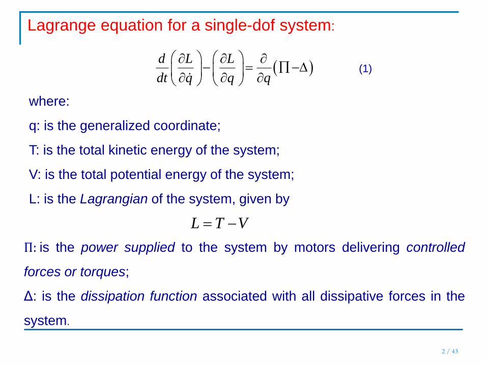
Lagrange equation for a single-dof system:

where:

q: is the generalized coordinate;

T: is the total kinetic energy of the system;

V: is the total potential energy of the system;

L: is the Lagrangian of the system, given by

Π: is the power supplied to the system by motors delivering controlled

forces or torques;

Δ: is the dissipation function associated with all dissipative forces in the

system.

d L L

dt q q q

L T V

(1)

3 / 9

a) Kinetic Energy of the 𝑖𝒕𝒉 Rigid Body of a Mechanical System

Undergoing Planar Motion

where:

𝑚𝑖 is the mass of the ith rigid body;

𝒄 𝑖 is the two-dimensional velocity vector of the center of mass of the

𝑖𝑡ℎ rigid body with respect to an inertial frame, ‖𝑐 𝑖‖ representing its

magnitude;

𝐼𝐶𝑖 is the scalar moment of inertia of the 𝑖𝑡ℎ rigid body with respect to

its center of mass; and 𝜔𝑖 is the scalar angular velocity of the ith

rigid body with respect to an inertial frame.

2 21 1

2 2i i i Ci iT m I c

T: Kinetic Energy

The kinetic energy 𝑇𝑖 of the 𝑖𝑡ℎ rigid body can be determined using ….

4 / 9

b) Kinetic Energy of the 𝑖𝒕𝒉 Rigid Body of a Mechanical

System Undergoing Planar Motion Based on a Fixed Point

O𝑖 of the Body

where:

𝐼𝑂𝑖 is the scalar moment of inertia of the 𝑖th rigid body with

respect to a point 𝑂𝑖 of the body that is instantaneously fixed to

an inertial frame;

𝜔𝑖 is the scalar angular velocity of the 𝑖th rigid body with

respect to an inertial frame.

The kinetic energy of the overall system is the sum of the kinetic

energies of all r rigid bodies, i.e.,

21

2i Oi iT I

1

r

iT T

The velocity vector of the center of mass of each body and its scalar

angular velocity can be always written as linear functions of the

generalized speed.

The total kinetic energy of the system takes the form:

2

0

1, ( , )

2T m q q p q t q T q t

where the coefficients 𝑚(𝑞) and 𝑝(𝑞, 𝑡) as well as 𝑇0(𝑞, 𝑡) are, in general, functions of

the generalized coordinate q. The first term of that expression is quadratic in the

generalized speed; the second term is linear in this variable; and the third term is

independent of the generalized speed, but is a function of the generalized coordinate

and, possibly, of time as well. Moreover, this function of q is most frequently nonlinear,

while the second and the third terms of the same expression arise in the presence of

actuators supplying a controlled motion to the system.

(2)

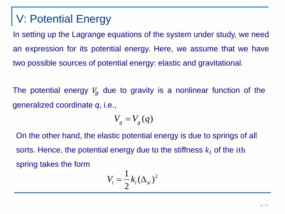
V: Potential Energy

6 / 9

In setting up the Lagrange equations of the system under study, we need

an expression for its potential energy. Here, we assume that we have

two possible sources of potential energy: elastic and gravitational.

The potential energy 𝑉𝑔 due to gravity is a nonlinear function of the

generalized coordinate q, i.e.,

( )g gV V q

On the other hand, the elastic potential energy is due to springs of all

sorts. Hence, the potential energy due to the stiffness 𝑘𝑖 of the 𝑖th

spring takes the form

21( )

2i i siV k

7 / 9

Δ𝑠𝑖 being the elongation or contraction of the 𝑖th spring. The foregoing

discussion applies to translational springs, a similar expression

applying to torsional springs:

21

2i ti iV k

Thus, under the assumption that the system has a total of s springs, the

total potential energy is given as

2

1

1

2

s

g i iV V k q

where 𝑘𝑖 can be either translational or torsional and 𝑞𝑖 is a

generalized coordinate.

8 / 9

Π and : Power Supplied to a System and

Dissipation Function

Single-dof systems have a single generalized force associated with

them. If we let the total power developed by force-controlled sources

be denoted by Π, then, the generalized active force ϕ𝑓 associated with

the generalized coordinate q is derived as

fq

where 𝑞 is the corresponding generalized velocity.

9 / 9

Systems are not only acted upon by driving forces but also by

dissipative forces that intrinsically oppose the motion of the system.

Here, we postulate the existence of a dissipation function Δ from

which the dissipative force ϕ𝑑 is derived as

dq

the negative sign taking into account that Δ is essentially a positive

quantity, while ϕ𝑑 opposes motion.

Dissipation of energy occurs in nature in many forms. The most

common mechanisms of energy dissipation are:

(a) viscous damping, (b) Coulomb or dry-friction damping,

(c) hysteretic damping,

The Seven Steps of the Modeling Process

10 / 9

We derive below the general form of the Lagrange equations, Eq. (1), as

pertaining to single-dof systems. To this end, we use Eq. (2) to derive the

Lagrangian in the form

2

0

1, ( , )

2L m q q p q t q T q t V q

Hence,

,L

m q q p q tq

and

2d L p pm q q m q q q

dt q q t

11 / 9

Likewise,

Moreover, the right-hand side of Eq. (1) is nothing but the sum of the

terms due to force-controlled sources and dissipation, i.e,

f dq

Therefore, the Lagrange equations take the form

2 0

,

1

2

pm

f d

h q q

Tp Vm q q m q q

t q q

In summary, then, the Lagrange equation for single-dof systems takes the

form

In summary, the Lagrange equation for single-dof systems takes the form

, , ,m q q h q q q q t

the governing model is a second-order ordinary differential equation in the

generalized coordinate q.

In this equation, the configuration-dependent coefficient m(q), the generalized

mass, while the second term of the left-hand side,

h(q,˙q), contains inertia forces stemming from Coriolis and centrifugal

accelerations. For this reason, this term is sometimes called the term of Coriolis

and centrifugal forces.

The right-hand side, in turn, is the sum of four different generalized-force terms,

namely,

(1) φp(q, t), a generalized force stemming from the potential energy of the

Lagrangian;

(2) (2) φm(q, ˙ q, t), a generalized force stemming from motion-controlled

sources and contributed by the Lagrangian as well;

(3) (3) φ f (q, ˙ q, t), a generalized force stemming from force-controlled

sources, and contributed by the power Π;

(4) (4) φd (q, ˙ q, t), a generalized force of dissipative forces, stemming from

the dissipation function Δ.

Sistemi Meccanici 12 / 9


13 / 9

Example 1.6.4 from Dynamics Response … by J. Angeles

A Locomotive Wheel Array

Derive the Lagrange equation of the system shown in Fig. This system consists of two identical

wheels of mass m and radius a that can be modeled as uniform disks. Furthermore, the two wheels

are coupled by a slender, uniform, rigid bar of mass M and length l, pinned to the wheels at points a

distance b from the wheel centers. We can safely assume that the wheels roll without slipping on the

horizontal rail and that the only nonnegligible dissipative effects arise from the lubricant at the bar-

wheel pins. These pins produce dissipative moments proportional to the relative angular velocity of

the bar with respect to each wheel.

14 / 9


Solution: Under the no-slip assumption, it is clear that a single

generalized coordinate, such as θ , suffices to describe the

configuration of the entire system at any instant. The system thus

has a dof = 1.

We introduce the seven-step procedure to derive the mathematical

model sought:

1. Kinematics

2. Kinetic energy

3. Potential energy

4. Lagrangian

5. Power supplied

6. Power dissipation

7. Lagrance Equation

15 / 9

1 /P P C v c v

3 1 /P C c c v

1. Kinematics.

if we denote by P the center of the pin connecting the wheel 1 with the

coupler bar, we have

where 𝒗𝑃 𝐶 denotes the relative velocity of P with respect to C1,


C3 has a velocity identical to 𝒗𝑃

16 / 9

all that we need to find 𝑇3 is ‖𝑐 3‖2

2 2 2 2 2 2

3 2 cosa b ab c

2. Kinetic energy

𝐼𝑖 denotes the moment of inertia of the 𝑖th body about its center of

mass 𝐶𝑖

2

1 2

1

2I I ma

2

3

1

12I Ml

As a matter of fact, 𝐼3 will not be needed because body 3 undergoes a pure

translation.


17 / 9

22 2 2 2 2

1 2

1 1 1 1 3

2 2 2 2 2

aT T ma ma m

2 2 2

3

12 cos

2T M a b ab

whence,

2 2 2 23 12 cos

2 2T ma M a ab b


18 / 9

3. Potential energy.

We note that the sole source of potential energy is gravity.

cosgV Mgb

4. Lagrangian.

This is now readily derived as

2 2 2 23 12 cos cos

2 2L T V ma M a ab b Mgb

5. Power supplied.

Apparently, the system is not subjected to any force-controlled

source, and hence, 𝛱 = 0.


19 / 9

6. Power dissipation.

What is important here is to find the angular velocity of the

bar with respect to each of the wheels

212

2c

7. Lagrange equation.

Now, all we need is to evaluate the partial derivatives involved in Eq.

1.22, namely,

2 2 23 2 cosL

ma M a ab b


20 / 9

Hence, 2 2 2 23 2 cos 2 sind L

ma M a ab b Mabdt

and 2sin sinL

Mab Mgb

Furthermore, 0

2c

the equation sought thus being

2 2 2 23 2 cos sin sin 2ma M a ab b Mab Mgb c

Thus, the generalized mass of the system is

2 2 23 2 cosm ma M a ab b


21 / 9

Likewise, the term of Coriolis and centrifugal forces is readily

identified as 2, sinh Mab

Finally, the right-hand side contains one term of gravity forces,

𝑀𝑔𝑏𝑠𝑖𝑛𝜃 , and one that is dissipative, 2𝑐𝜃 . The only driving force here

is gravity, and this is taken into account in the Lagrangian. We thus

have

sinp Mgb

0m f 2d c


22 / 9


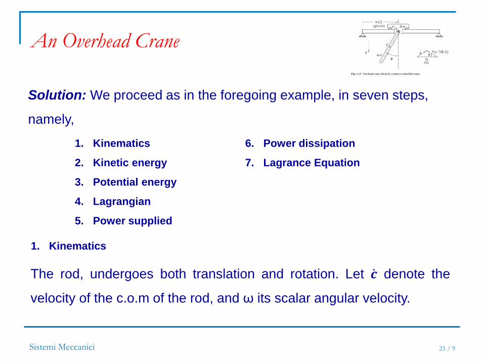
An Overhead Crane

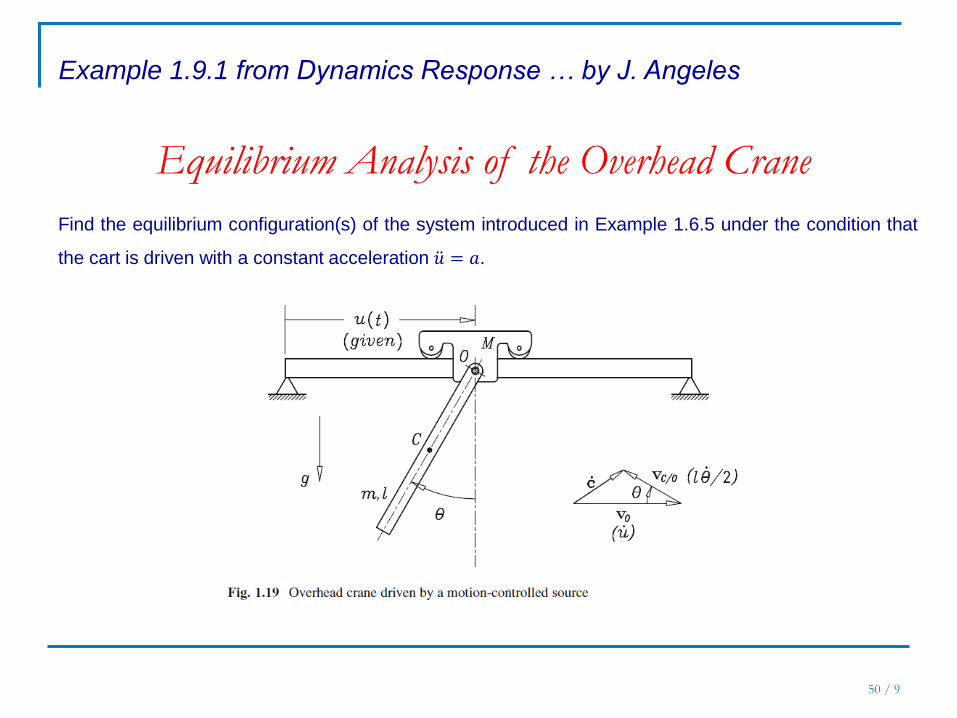
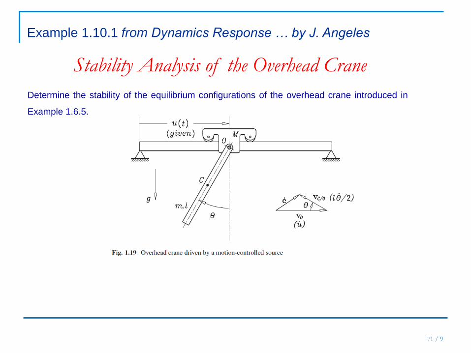
Now we want to derive the Lagrange equation of the overhead crane of Fig. 1.19 that consists of a

cart of mass M that is driven with a controlled motion u(t). A slender rod of length l and mass m is

pinned to the cart at point O by means of roller bearings producing a resistive torque that can be

assumed to be equivalent to that of a linear dashpot of coefficient c.


The rod, undergoes both translation and rotation. Let 𝒄 denote the

velocity of the c.o.m of the rod, and ω its scalar angular velocity.

Solution: We proceed as in the foregoing example, in seven steps,

namely,

1. Kinematics

2. Kinetic energy

3. Potential energy

4. Lagrangian

5. Power supplied



1. Kinematics

An Overhead Crane

24 / 9

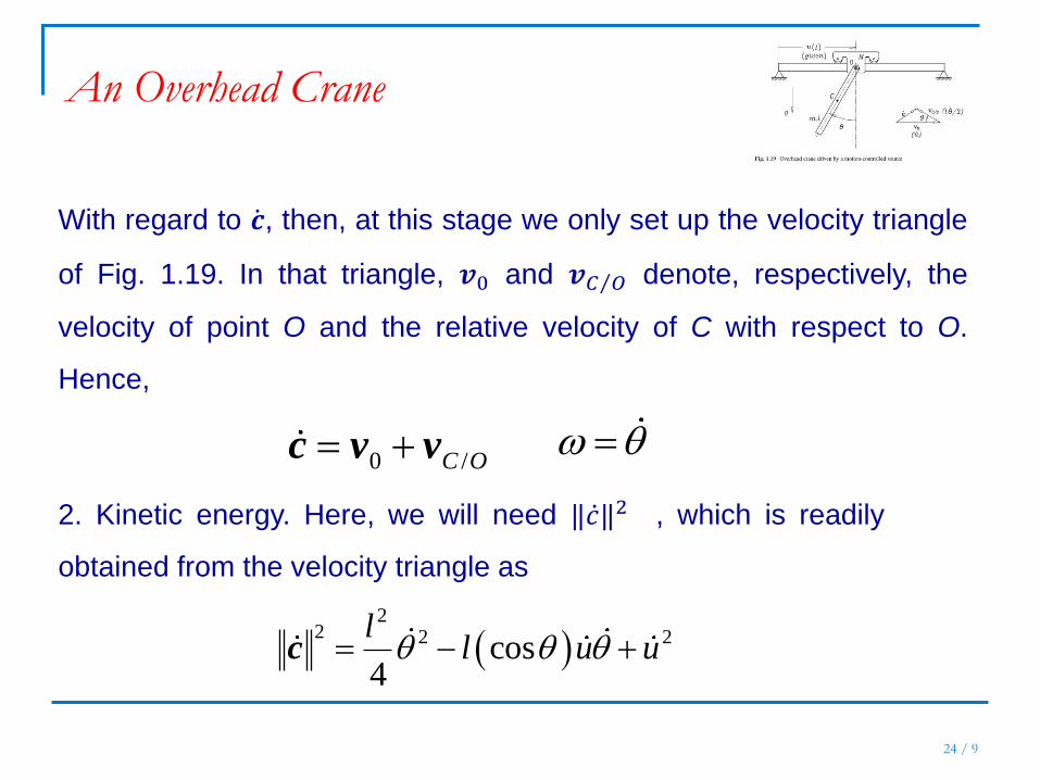
With regard to 𝒄 , then, at this stage we only set up the velocity triangle

of Fig. 1.19. In that triangle, 𝒗0 and 𝒗𝐶 𝑂 denote, respectively, the

velocity of point O and the relative velocity of C with respect to O.

Hence,

0 /C O c v v

2. Kinetic energy. Here, we will need ‖𝑐 ‖2 , which is readily

obtained from the velocity triangle as

2

2 2 2cos4

ll u u c

An Overhead Crane

25 / 9

Now, let 𝑇𝑐 and 𝑇𝑟 denote the kinetic energies of the cart and the

rod, respectively, i.e., 21

2cT Mu

2 2 2 2 2 2 2 21 1 1 1 1 1cos cos

2 4 2 12 2 3rT m l l u u ml m l l u u

and hence,

2 2 21 1 1cos

2 3 2T m l l u M m u

Compared with Eq. 1.27, the foregoing expression yields

1

, cos2

p t ml u t 2

0

1

2T t M m u

An Overhead Crane

26 / 9

3. Potential energy.

This is only gravitational and pertains to the rod, the potential

energy of the cart remaining constant, and, therefore, can be

assumed to be zero. Hence, if we use the level of the pin as a

reference, cos

2g

lV mg

4. Lagrangian. This is simply

2 2 21 1 1cos cos

2 3 2 2

lL m l l u M m u mg

5. Power supplied. Again, we have no driving force, and

hence, 𝛱 = 0.

An Overhead Crane

27 / 9

6. Power dissipation. Here, the only sink of energy occurs in the pin,

and hence, 21

2c

7. Lagrange equations. Now it is a simplematter to calculate

the partial derivatives of the foregoing functions:

21 1cos

3 2

Lml ml u

21 1 1sin cos

3 2 2

d Lml ml u ml u

dt

1 1

sin sin2 2

Lml u mgl

An Overhead Crane

28 / 9

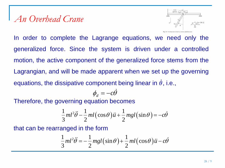
In order to complete the Lagrange equations, we need only the

generalized force. Since the system is driven under a controlled

motion, the active component of the generalized force stems from the

Lagrangian, and will be made apparent when we set up the governing

equations, the dissipative component being linear in 𝜃 , i.e.,

d c

Therefore, the governing equation becomes

21 1 1cos sin

3 2 2ml ml u mgl c

that can be rearranged in the form

21 1 1sin cos

3 2 2ml mgl ml u c

An Overhead Crane

29 / 9

Now we can readily identify the generalized mass as

21

3m ml

Likewise,

, 0h

and so, the system at hand contains neither Coriolis nor centrifugal forces.

An Overhead Crane

30 / 9

1

sin2

p mgl 1

, cos2

m t ml u

0f d c

An Overhead Crane

Finally, the right-hand side is composed of three terms: (1) a gravity term

𝜙𝑝 𝜃 that is solely a function of θ , but not of 𝜃 ; (2) a generalized active

force 𝜙𝑚 𝜃, 𝑡 that is provided by a motion-controlled source, i.e., the motor

driving the cart with a controlled displacement u(t); and (3) a dissipative

term. All these terms are displayed below:


Describe how the mathematical model of Example 1.6.5 changes if the pin is substituted by a motor

that supplies a controlled torque 𝜏 𝑡 , in order to control the orientation of the rod for purposes of

manipulation tasks. Here, we assume that this torque is accompanied by a dissipative torque linear in

𝜃 , as in Example 1.6.5.


A Force-driven Overhead Crane

32 / 9

Solution: The motor-supplied torque now produces a power

𝛱 = 𝜏 𝑡 𝜃 𝑡 onto the system, the generalized force now containing

an active controlled-force component 𝜙𝑓 𝜃, 𝜃 , 𝑡 , namely,

, ,f t t

21 1 1sin cos

3 2 2ml mgl t ml u c

all other terms remaining the same. Therefore, the governing

equation becomes now

A Force-driven Overhead Crane

33 / 9

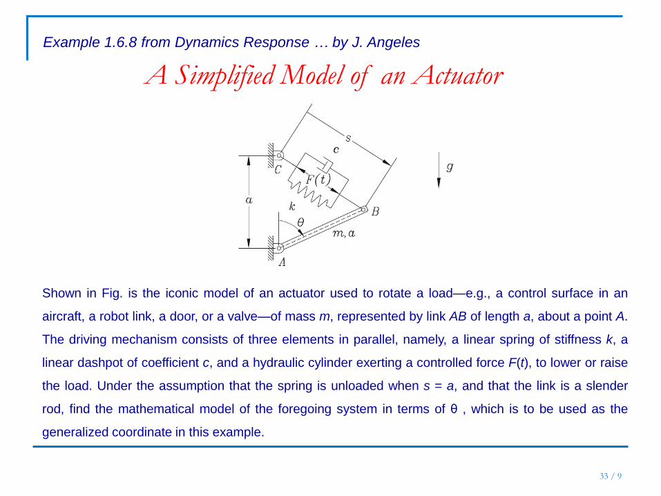
Shown in Fig. is the iconic model of an actuator used to rotate a load—e.g., a control surface in an

aircraft, a robot link, a door, or a valve—of mass m, represented by link AB of length a, about a point A.

The driving mechanism consists of three elements in parallel, namely, a linear spring of stiffness k, a

linear dashpot of coefficient c, and a hydraulic cylinder exerting a controlled force F(t), to lower or raise

the load. Under the assumption that the spring is unloaded when s = a, and that the link is a slender

rod, find the mathematical model of the foregoing system in terms of θ , which is to be used as the

generalized coordinate in this example.


A Simplified Model of an Actuator

34 / 9

Solution: We proceed as in the previous cases, i.e., following the

usual seven-step procedure:


1. Kinematics

2. Kinetic energy

3. Potential energy

4. Lagrangian

5. Power supplied




1. Kinematics

Besides the foregoing item, we will need a relation between the length of

the spring, s, and the generalized variable,θ . This is readily found from

the geometry of Fig. 1.21, namely,

2 sin2

s a

2. Kinetic energy.

2 21 1

2 2A AT I I


36 / 9

21

3AI ma

Thus, 2 21

6T ma

3. Potential energy. We now have both gravitational and

elastic forms of potential energy. If we take the horizontal

position of AB as the reference level to measure the potential

energy due to gravity, then

21

cos2 2

aV mg k s a


37 / 9

or, in terms of the generalized coordinate alone, 2

1cos 2 sin

2 2 2

aV mg k a a

4. Lagrangian. This is simply 2

21 1cos 2 sin

6 2 2 2

aL T V ma mg k a a

5. Power supplied. The system is driven under a controlled force

F(t) that is applied at a speed ˙ s, and hence, the power supplied

to the system is

F t s


38 / 9

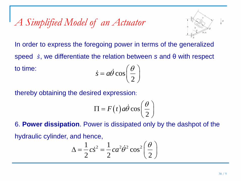
In order to express the foregoing power in terms of the generalized

speed 𝑠 , we differentiate the relation between s and θ with respect

to time: cos

2s a

thereby obtaining the desired expression:

cos2

F t a

6. Power dissipation. Power is dissipated only by the dashpot of the

hydraulic cylinder, and hence,

2 2 2 21 1cos

2 2 2cs ca


39 / 9

7. Lagrange equations. We first evaluate the partial derivatives of

the Lagrangian:

21

3

Lma

21

3

d Lma

dt

2

2

sin 2sin 1 cos2 2 2

sin cos 2sin 1 cos2 2 2 2

L amg ka

amg ka

where we have written all partial derivatives in terms of angle θ /2.

Furthermore,

cos2

F t a

2 2cos2

ca


40 / 9

the equation sought thus being

212sin 1 sin cos cos cos

3 2 2 2 2 2ma a ka mg F t a ca

The generalized mass can be readily identified from the above

model as 21

3m ma

Also note that the generalized-force terms are identified below

as:

2 sin cos2 2

p a ka mg ka

while


41 / 9

cos2

d ca

cos2

f F t a

0m

Finally, the equation of motion can be rearranged as

33 3

2 sin cos cos cos2 2 2 2

F t cka mg ka

ma ma ma


42 / 9

Shown in Fig. is a highly simplified model of the actuator mechanism of an aircraft control surfacee.g.,

ailerons, rudder, etc. In the model, a massless slider is positioned by a stepper motor at a displacement

u(t). The inertia of the actuator-aileron system is lumped in the rigid, slender, uniform bar of length l and

mass m, while all the stiffness and damping is lumped in a parallel spring-dashpot array whose left end A is

pinned to a second massless slider that can slide without friction on a vertical guideway. Moreover, it is

known that the spring is unloaded when u = l and θ = 0. A second motor, mounted on the first slider, exerts

a torque τ (t) on the bar.


Motion-driven Control Surface

43 / 9

(a) Derive the Lagrangian of the system.

(b) Give expressions for the power 𝛱 supplied to the system and for

the dissipation function Δ.

(c) Obtain the mathematical model of the system and identify in it the

generalized forces (1) supplied by force-controlled sources; (2)

supplied by motion controlled sources; (3) stemming from potentials;

and (4) produced by dissipation.


1. Kinematics

2. Kinetic energy

3. Potential energy

4. Lagrangian

5. Power supplied



44 / 9

Solution:

(a) The kinetic energy of the system is that of the overhead

crane of Example 1.6.5, except that now the cart has negligible

mass, i.e., M = 0, and hence,

The potential energy is the same as that of Example 1.6.5 plus the

elastic energy 𝑉𝑒 of the spring, which is

2 2 21 1 1cos

2 3 2T m l l u t mu t

21

2eV k s l

Moreover, from the geometry of Fig. 1.22,


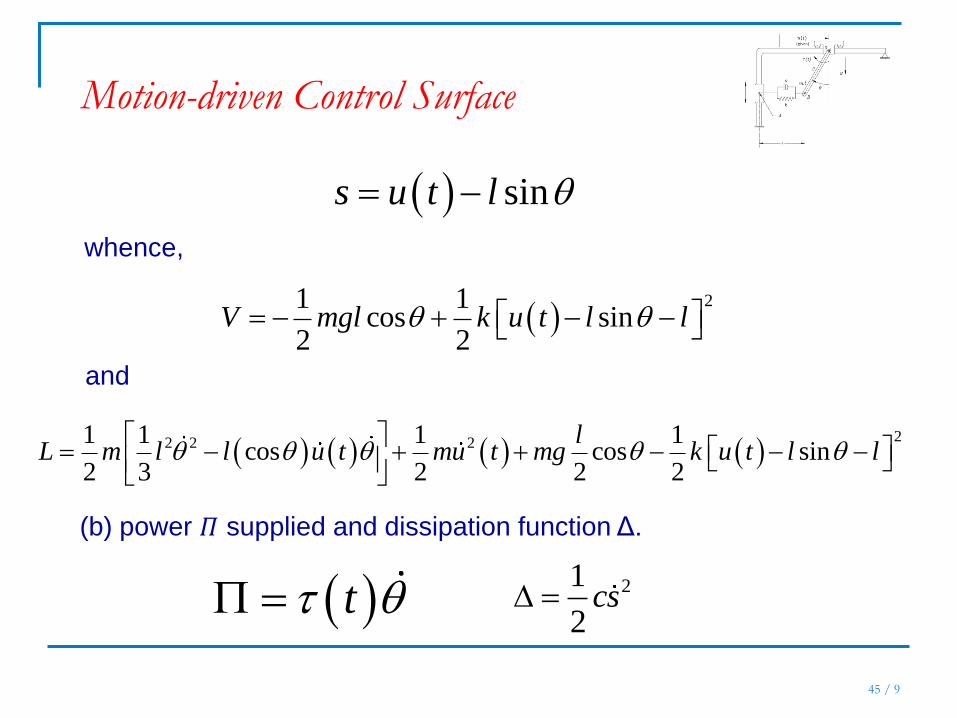
45 / 9

sins u t l

whence,

21 1

cos sin2 2

V mgl k u t l l

and

22 2 21 1 1 1

cos cos sin2 3 2 2 2

lL m l l u t mu t mg k u t l l

(b) power 𝛱 supplied and dissipation function Δ.

t 21

2cs


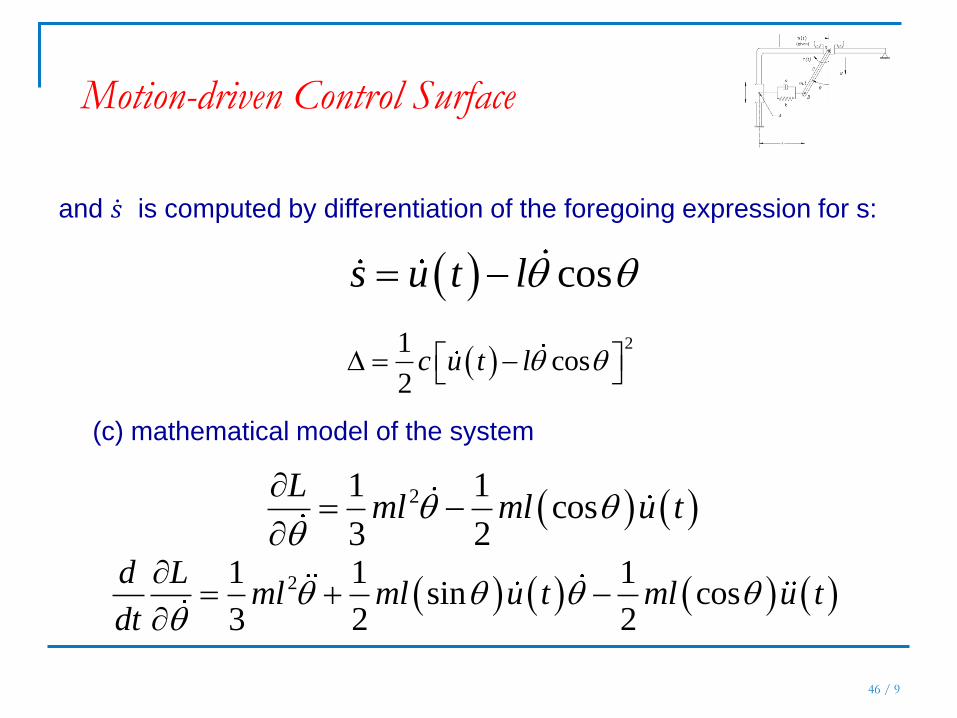
46 / 9

and 𝑠 is computed by differentiation of the foregoing expression for s:

coss u t l

21

cos2

c u t l

(c) mathematical model of the system

21 1cos

3 2

Lml ml u t

21 1 1sin cos

3 2 2

d Lml ml u t ml u t

dt


47 / 9

1 1

sin sin sin cos2 2

Lml u t mgl kl u t l l

1 1

sin sin sin cos2 2

Lml u t mgl k u t l l l

t

cos cos cos cosc u t l l cl l u t


48 / 9

Thus, the mathematical model is derived as

21 1 1 1sin cos sin

3 2 2 2

1sin sin cos cos cos

2

ml ml u t ml u t ml u t

mgl kl u t l l t cl l u t

or,

2

2 2 2

1 1cos cos cos

3 2

1sin 1 sin cos cos

2

ii

iiiivi

ml ml u t clu t klu t

mgl kl t cl


Equilibrium States of Mechanical

Systems

49 / 9

Henceforth, a mechanical system will be said to be in an equilibrium state

if both 𝑞 = 0 and 𝑞 = 0. This condition implies that, at equilibrium, q attains

a constant value 𝑞𝐸.

we derive the equilibrium equation in the form

,0 0Eq

50 / 9

Find the equilibrium configuration(s) of the system introduced in Example 1.6.5 under the condition that

the cart is driven with a constant acceleration 𝑢 = 𝑎.


Equilibrium Analysis of the Overhead Crane


Solution: We first set 𝑢 = 𝑎, 𝜃 = 0 and 𝜃 = 0 in the governing equation

derived in that example, thereby obtaining the equilibrium equation

1 1

sin cos 02 2

E Emgl ml a

which can be written as

tan E

a

g


52 / 9

and hence,

1tanE

a

g

The system, therefore, admits two equilibrium configurations, one

with the rod above and one with the rod below the pin.

The foregoing relation among the constant horizontal

acceleration a, the vertical gravity acceleration g and the equilibrium

angle 𝜃𝐸 is best illustrated in Fig. 1.30, where the force triangle,

composed of the pin force 𝑓𝑃, the weight of the rod mg, and the

inertia force −ma, is sketched.

Pf


53 / 9

Moreover, from Fig. 1.30, it is apparent that

2 2cos E

g

a g

2 2sin E

a

a g


54 / 9

Determine all the equilibrium states of the actuator mechanism introduced in Example 1.6.8.


Equilibrium States of the Actuator Mechanism

To this end, assume that

2 2mg

ka 0F t


2 sin cos 02 2

E Eka mg ka

Solution: Upon setting 𝜃 = 𝜃𝐸 , 𝜃 = 0, and 𝜃 = 0 in the mathematical

model derived in Example 1.6.8, the equilibrium equation is obtained as


2sin cos 0

2 2 2

E E

2 sin 1 cos 02 2

E E

56 / 9

which vanishes under any of the conditions given below:

2sin

2 2

E cos 0

2

E

That is, equilibrium is reached whenever 𝜃𝐸 attains any of the

three values given below:

90E 180 270


57 / 9

The foregoing values yield the equilibrium configurations of Fig. 1.31.

58 / 9

Example 1.9.4 (A System with a Time-varying Equilibrium State).

Derive the equilibrium states of the rack-and-pinion transmission of

Fig. 1.3.

59 / 9

Solution: Let us assume that the moment of inertia of the pinion about its

center of mass is I, and that its mass is m, its radius being a. Thus, the

velocity of its c.o.m is 𝑎𝜃 , and hence, the kinetic energy becomes

a

2 2 2 2 21 1 1

2 2 2T ma I I ma

Moreover, no changes in the potential energy are apparent, since

the center of mass of the pinion remains at the same level, and

hence, we can set V = 0, which leads to L = T in this case. Now the

Lagrange equation of the system is, simply,

2 2 0I ma

and hence, the equilibrium equation, obtained when we set 𝜃 = 0,

becomes an identity, namely, 0 = 0.

Linearization About Equilibrium

States. Stability

60 / 9

If a system is in an equilibrium state and is perturbed slightly, then,

the system may respond in one of three possible ways:

• The system returns eventually to its equilibrium state

• The system never returns to its equilibrium state, from

which it wanders farther and farther

• The system neither returns to its equilibrium state nor

escapes from it; rather, the system oscillates about the

equilibrium state In the first case, the equilibrium state is said to be stable or, more precisely, asymptotically stable; in the

second case, the equilibrium state is unstable or asymptotically unstable. The third case is a borderline

case between the two foregoing cases. This case, then, leads to what is known as a marginally stable

equilibrium state.

61 / 9

We analyze below a single-dof system governed by the equation


Thus, we denote the value of q at its equilibrium state by 𝑞𝐸 and

linearize the system about this state, as described below.

Moreover, at equilibrium, 𝑞 = 0

First, we perturb slightly the equilibrium state,

Eq q q q q q q

Otherwise, one can resort to a series expansion.

62 / 9

, , ,0,E E

E E

q q q t q t q q tq q

, ,0E E

E E

h hh q q q h q q q

q q

E E Em q q m m q q

where the subscripted vertical bar indicates that the quantity to its

left is evaluated at equilibrium.

At the equilibrium

E Em m q

63 / 9

An equilibrium configuration is understood throughout the book as a

configuration of the system governed by 𝑞 = 𝑞𝐸 , at which we have

assumed that 𝑞 = 0 . In evaluating the partial derivatives of h with

respect to q and 𝑞 at equilibrium, we have:

210

2 EE

hm q q

q

0

EE

hm q q

q

Therefore, , 0Eh q q q

substituting

E E

E E

m m q q q q q tq q

Under the small-perturbation assumption, the quadratic term involving the product

in the left-hand side of the above equation is too small with respect to the linear terms,

and hence, is neglected.

64 / 9

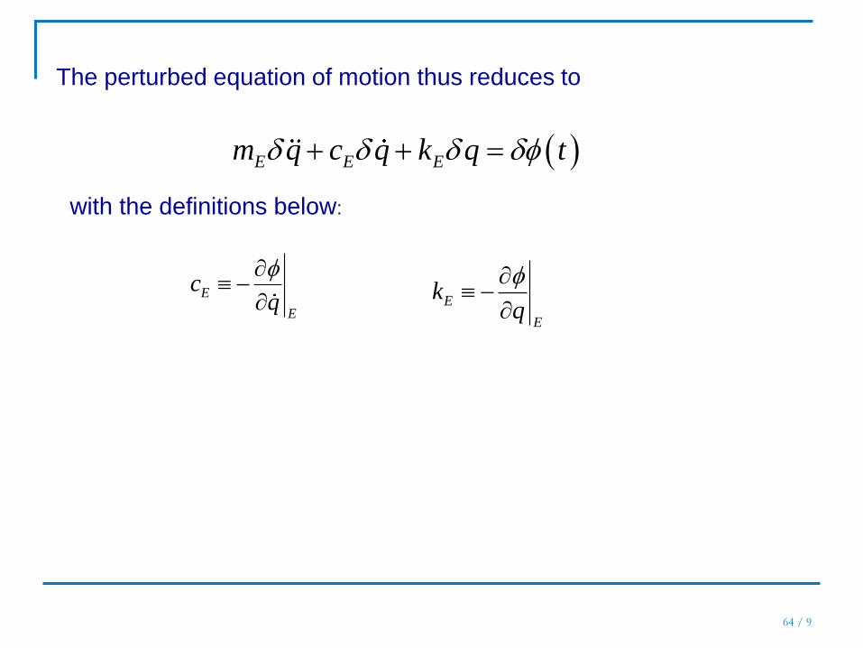
The perturbed equation of motion thus reduces to

E E Em q c q k q t

with the definitions below:

E

E

cq

E

E

kq

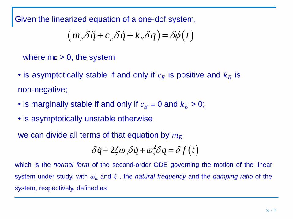
65 / 9

Given the linearized equation of a one-dof system,

E E Em q c q k q t

where mE > 0, the system

• is asymptotically stable if and only if 𝑐𝐸 is positive and 𝑘𝐸 is

non-negative;

• is marginally stable if and only if 𝑐𝐸 = 0 and 𝑘𝐸 > 0;

• is asymptotically unstable otherwise

we can divide all terms of that equation by 𝑚𝐸

22 n nq q q f t

which is the normal form of the second-order ODE governing the motion of the linear

system under study, with 𝜔𝑛 and 𝜉 , the natural frequency and the damping ratio of the

system, respectively, defined as

66 / 9

En

E

k

m

2 2

E E

E n E E

c c

m k m

E

tf t

m

For brevity ,we shall write in a simpler form, i.e., by dropping the

subscript E and the δ symbol, whenever the equilibrium configuration is

either self-understood or immaterial, namely,

SSSSSSSSSSSSSS

or, in normal form, as

¨ q+2ζωn ˙ q+ω2 with ωn and ζ defined now as

and, obviously, f (t) defined as

f (t) ≡ φ (t)/m.

The mathematical model appearing in Eq. 1.57 corresponds to the

iconic model

of Fig. 1.34m


SSSSSSSSSSSSSS

68 / 9

A Mass-spring-dashpot System in a Gravity Field

69 / 9

In Fig. 1.36a the system is displayed with the spring unloaded, while

the same system is shown in its static equilibrium position in Fig. 1.36b,

this position being that at which the spring force balances the weight of

the mass, and hence,

k s mg

Application of Newton’s equation in the vertical direction now gives

mx mg k x s cx mg k s kx cx

Thus, the equilibrium equation derived above reduces to

0mx cx kx

Example 1.10.4 (A Mass-spring-dashpot System in a Gravity Field). Illustrated in Fig. 1.36 is a mass-

spring-dashpot system suspended from a rigid ceiling. For this system, discuss the difference in the

models resulting when the displacement of the mass is measured (a) from the configuration where the

spring is unloaded and (b) from the static equilibrium configuration.

70 / 9

If, rather than measuring the displacement of the mass from

equilibrium, we measure it from the position in which the spring is

unloaded, then we set up the governing equation in terms of the new

variable ξ , defined as

x s

Upon substituting in the governing equation derived above, we have

m c k k s

71 / 9

Determine the stability of the equilibrium configurations of the overhead crane introduced in

Example 1.6.5.


Stability Analysis of the Overhead Crane


3 3

sin cos2 2

E E

g a

l l

which leads to

Solution: In order to undertake the stability analysis of the equilibrium

configurations of the system under study, we make the substitutions given

below in the governing equation derived in Example 1.6.5, with 𝑢 = 𝑎 =

const and c = 0 (neglect dissipation). We have

E


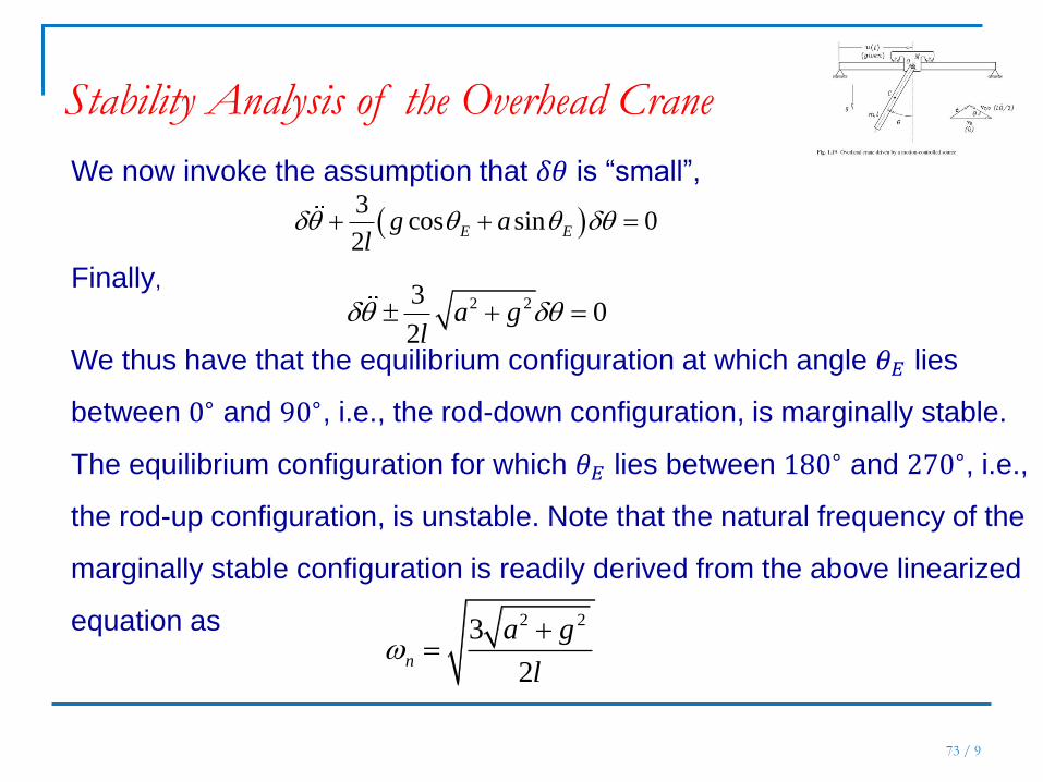
73 / 9

3

cos sin 02

E Eg al

We now invoke the assumption that 𝛿𝜃 is “small”,

Finally, 2 23

02

a gl

We thus have that the equilibrium configuration at which angle 𝜃𝐸 lies

between 0∘ and 90∘, i.e., the rod-down configuration, is marginally stable.

The equilibrium configuration for which 𝜃𝐸 lies between 180∘ and 270∘, i.e.,

the rod-up configuration, is unstable. Note that the natural frequency of the

marginally stable configuration is readily derived from the above linearized

equation as


2 23

2n

a g

l

74 / 9

Decide whether each of the equilibrium configurations of Fig. 1.31, of the actuator mechanism, found in

Example 1.9.2 is stable or unstable, when the system is unactuated—i.e., when F(t) = 0. For the stable

cases, whether stability is asymptotic or marginal, and find, in each case, the equivalent natural

frequency and, if applicable, the damping ratio.


Stability Analysis of the Actuator Mechanism


Solution: What we have to do is linearize the governing equation

about each equilibrium configuration, with F(t) = 0. To do this, we

substitute the values below into the Lagrange equation of the

system at hand:

E The equation of motion thus becomes

2 33 2 sin cos cos

2 2 2 2

E E Ek c

m ma

0F t

We analyze below each of the three equilibrium configurations

found in Example 1.9.2:


76 / 9

(a 𝜃𝐸 =𝜋

2: In this case,

2sin sin 1

2 4 2 2 2

E

2cos cos 1

2 4 2 2 2

E

the linearized equation about the equilibrium configuration

considered here thus becoming, after simplifications,

3 2 3 21 1

2 2 2 2 2

k c

m ma


77 / 9

Upon dropping the quadratic terms of the above expression, and

rearranging the expression thus resulting in normal form, we obtain

3 2 3 20

2 2 2

c k

ma m

The natural frequency and the damping ratio associated with the

linearized system are thus

3 2

2n

k

m

3 2 2

4 3

c

a km


78 / 9

(b) 𝜃𝐸 = 𝛱: now we have

sin sin 12 2 2

E

Upon substitution of the foregoing values into the Lagrange

equation, we obtain, after simplification,

Next, we delete the quadratic terms from the above equation, and

rewrite it in normal form, thus obtaining

2 2 23 0

2 2

k

m

(c) 𝜃𝐸 = 3𝛱 2 : this configuration is the mirror-image of the first

one, 𝜃𝐸 = 𝛱 2


Date post:	02-May-2020
Category:	Documents
Upload:	others
View:	2 times
Download:	1 times

The Modeling of Single-dof Mechanical Systems · We derive below the general form of the Lagrange...

Documents