The modified Helmholtz equation

in a semi-strip

Y.A. Antipov1, A.S. Fokas2

1Department of Mathematics, Louisiana State University

Baton Rouge, LA 70803, U.S.A.∗

antipov@math.lsu.edu2Department of Applied Mathematics and Theoretical Physics,

University of Cambridge, Silver Street, Cambridge CB3 9EW, U.K.

T.Fokas@damtp.cam.ac.uk

Submitted to Math. Proc. Cambridge Phil. Soc.

Abstract

We study the modified Helmholtz equation in a semi-strip with Poincare typeboundary conditions. On each side of the semi-strip the boundary conditions involvetwo parameters and one real-valued function. Using a new transform method re-cently introduced in the literature we show that the above boundary-value problemis equivalent to a 2 × 2-matrix Riemann-Hilbert (RH) problem. If the six parame-ters specified by the boundary conditions satisfy certain algebraic relations this RHproblem can be solved in closed form. For certain values of the parameters the solu-tion is not unique, furthermore in some cases the solution exists only under certainrestrictions on the functions specifying the boundary conditions. The asymptoticsof the solution at the corners of the semi-strip is investigated. In the case that the2×2 RH problem cannot be solved in closed form, the Carleman-Vekua method forregularising it is illustrated by analysing in details a particular case.

∗The address to which mail should be sent

1

1 Introduction

A new method for studying boundary value problems for integrable PDE’s in two dimen-sional domains (x, y) has been introduced recently and reviewed in [1]. Examples ofintegrable equations are linear PDE’s with constant coefficients and the usual integrablenonlinear PDE’s such as the Korteweg-de Vries equation.

Let q(x, y) satisfy a second order linear elliptic PDE with constant coefficientsin a convex polygon in the complex z-plane, z = x + iy. This polygon can be ei-ther bounded with corners z1, . . . , zm, zm+1 = z1, or unbounded with corners z1 =∞, z2, . . . , zm−1, zm = ∞. On each side of the polygon, namely on the side (zj+1, zj)referred to as the side (j), let q(x, y) satisfy Poincare type boundary conditions

∂q

∂ν

∣

∣

∣

∣

ej

+ γjq = gj , (1.1)

where ∂q∂ν

∣

∣

∣

ej

= ∇q · ej is the outward directional derivative in the direction ej specified

by the constant βj (see Fig.1), γj is a real non-negative constant, and gj is a real-valuedfunction with appropriate smoothness and decay. The main steps of the method consistsof:

(1) Construct an integral representation in the complex k-plane for q(x, y) in termsof a certain function ρ(k) = ρj(k)

m1 called the spectral function. The function ρj(k)

is expressed as an integral over the side (j) involving q, qs, qn, where qs, qn are thetangential and the normal derivatives of the function q. Thus from (1.1) and integrationby parts it follows that each ρj involves one unknown boundary value.

(2) Use the fact that ρ(k) satisfies a certain global relation to characterise the partof ρ(k) involving the unknown boundary values in terms of βj , γj , gj

m1 . For a general

m-gon with the boundary conditions (1.1), this involves the formulation of a matrixRiemann-Hilbert (RH) problem.

Regarding this method we note that the formulae for ρ(k) and for q(x, y) are gen-eralised direct and inverse Fourier transforms respectively, ’custom made’ for the givenPDE and the given polygon. We also emphasise that for simple polygons and for alarge class of boundary conditions the above RH problem can be reduced to either atriangular RH problem (which can be solved in closed form), or to two separate scalarproblems; we will refer to such cases as triangular and scalar cases, respectively. In someparticular cases, the scalar RH problems can be bypassed all together, and ρ(k) can beobtained using only algebraic manipulations; we will refer to such cases as algebraiccases. It turns out that both the Dirichlet and the Neumann problems belong to thesealgebraic cases.

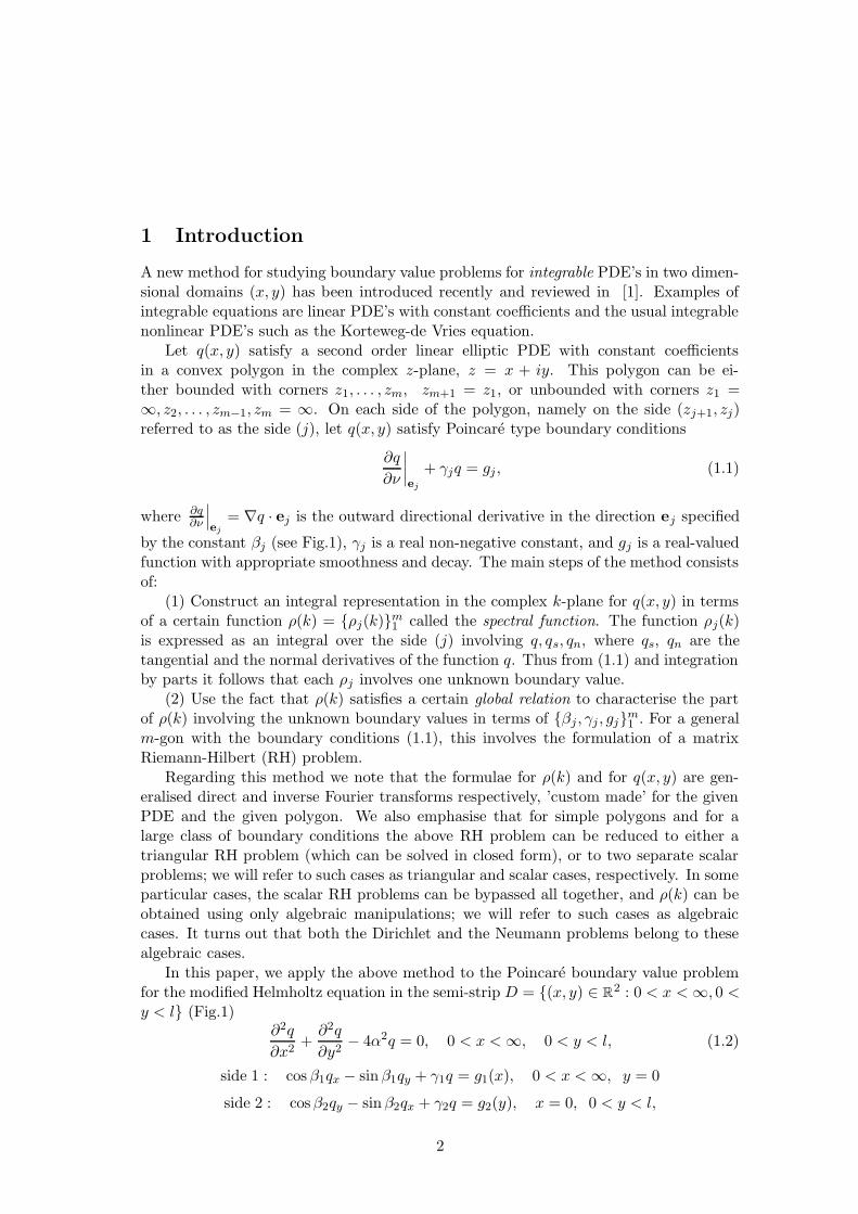
In this paper, we apply the above method to the Poincare boundary value problemfor the modified Helmholtz equation in the semi-strip D = (x, y) ∈ R

2 : 0 < x <∞, 0 <y < l (Fig.1)

∂2q

∂x2+∂2q

∂y2− 4α2q = 0, 0 < x <∞, 0 < y < l, (1.2)

side 1 : cos β1qx − sinβ1qy + γ1q = g1(x), 0 < x <∞, y = 0

side 2 : cosβ2qy − sinβ2qx + γ2q = g2(y), x = 0, 0 < y < l,

2

β

β

3

3

1

2 β2

l

y

x

e

e

e1

0

Figure 1: Geometry of the problem.

side 3 : cos β3qx + sinβ3qy + γ3q = g3(x), 0 < x <∞, y = l, (1.3)

where α is a real constant, γj are real non-negative constants, and 0 < βj < π (j =1, 2, 3). The functions g1(x), g3(x) vanish at the points x = 0 and x = ∞.

Let z1 = ∞ + i0, z2 = 0, z3 = il, z4 = ∞ + il. It is shown in [2] that the gener-alised direct and inverse Fourier transform pair associated with the modified Helmholtzequation

∂2

∂z∂z− α2q = 0, (1.4)

in the semi-strip with the end-points z1, z2, z3, z4, are given by:

ρj(k) =

zj∫

zj+1

e−(ikz+ α2

ikz)

(

qzdz +iα2

kqdz

)

, Im(k) ≤ 0 for j = 1, 3 and k ∈ C for j = 2,

(1.5)

3

and

q =1

2πi

3∑

j=1

∫

lj

eikz+ α2

ikzρj(k)

dk

k, 0 < x <∞, 0 < y < l, (1.6)

where the contours lj are the rays

l1 = k ∈ C : arg k = 0, l2 = k ∈ C : arg k = 12π, l3 = k ∈ C : arg k = π,

(1.7)directed away from the origin.

Furthermore, the spectral function ρ(k) = ρj(k)31 satisfies the global relation

3∑

j=1

ρj(k) = 0, Im(k) ≤ 0. (1.8)

For the semi-strip D and the boundary conditions (1.3), the analysis of the globalrelations gives rise to a matrix RH problem on the real axis.

The main aims of this paper are:(1) To derive the associated matrix RH problem.(2) To solve this RH problem in closed form in the triangular and scalar cases.(3) To analyse and solve the matrix RH problem corresponding to the Laplace equa-

tion, as a particular case of the Helmholtz equation.The paper is organised as follows. In Section 2 we review the method of [1] and use

the simple case of the Dirichlet boundary conditions to illustrate the main ideas. ThePoincare boundary-value problem for the modified Helmholtz equation in the semi-stripD is reduced to a 2 × 2 matrix RH problem on the real axis in Section 3. In Section 4,the scalar cases are analysed, namely it is shown that if

β1 + β2 =π

2m, (2α2 − γ2

2) = (2α2 − γ21)(−1)m−1, m = 1, 2, 3, (1.9)

and

β2 − β3 =π

2n, (2α2 − γ2

2) = (2α2 − γ23)(−1)n−1, n = −1, 0, 1, (1.10)

then the coupled 2× 2 RH problem can be reduced to two separate scalar RH problemswhich can be solved in closed form. In Section 5 the triangular cases are analysed,namely it is shown that if either of the conditions (1.9) or (1.10) is valid, then thematrix RH problem can be mapped to a triangular RH problem which can be solvedin closed form. In Section 6.1 the matrix RH problem associated with the Laplaceequation in the case β2 = 1

2(β3 − β1) is solved in closed form when all the parameters

γj (j = 1, 2, 3) are equal to zero; in Section 6.2 it is assumed that γ21 + γ2

2 + γ23 6= 0 and

the relevant matrix RH problem is regularised by the Carleman-Vekua method [5].

2 Basic notations and the Dirichlet problem

For elliptic equations it is convenient to replace the usual Cartesian coordinates (x, y)with the complex coordinates (z, z) = (x + iy, x − iy). For example, the modified

4

Helmholtz equation (1.2) can be written as

∂2q

∂z∂z− α2q = 0. (2.1)

An equation in two dimensions is called integrable if and only if it can be expressed asthe condition that a certain associated 1-form W (x, y, k), k ∈ C, is closed, i.e. dW = 0.A closed 1-form associated with an arbitrary linear PDE with constant coefficients isgiven in [4]. For example, a closed 1-form for the modified Helmholtz equation (1.2) is

W (z, z, k) = e−ikz+ iα2

kz

(

qzdz +iα2

kqdz

)

, k ∈ C. (2.2)

Indeed,

dW =

(

e−ikz+ iα2

kzqz

)

zdz ∧ dz +

(

iα2

ke−ikz+ iα2

kzq

)

z

dz ∧ dz

= e−ikz+ iα2

kz

[(

qzz +iα2

kqz

)

dz ∧ dz +

(

iα2

kqz + α2q

)

dz ∧ dz

]

. (2.3)

Thus, using dz ∧ dz = −dz ∧ dz, it follows that

dW = e−ikz+ iα2

kz(

qzz − α2q)

dz ∧ dz. (2.4)

Hence W is closed if and only if q(z, z) satisfies the modified Helmholtz equation (2.1).Suppose that the integrable equation satisfied by q(z, z) is valid in a simply connected

domain D with the boundary ∂D. The equation dW = 0 implies∫

∂D

W (z, z, k) = 0, k ∈ C. (2.5)

Following [2] we will refer to this equation as the global relation. For example, supposethat q(z, z) satisfies the modified Helmholtz equation in the semi-strip D. Then theglobal relation (2.5) becomes equation (1.8), where ρj(k) are defined by (1.5).

The above discussion indicates that both the global relation and the definition ofρ(k) are a direct consequence of the closed 1-form W (z, z, k). It was shown in [2] thatthe global relation can be used to characterise the unknown part of ρ(k), i.e. the partof ρ(k) that involves the unknown boundary values. This suggests that it is desirableto express q(z, z) directly in terms of ρ(k) (and not in terms of the boundary valuesthemselves). For the modified Helmholtz equation this expression is given by equation(1.6).

Such expressions can be derived either by using the spectral analysis of the closed1-form W [2], or by using the so-called fundamental differential form (which is a slightgeneralisation of W ) and a reformulation of Green’s formula [4].

We now use the Dirichlet problem to illustrate the method [1].

Example 2.1. Let the real valued function q(x, y) satisfy the modified Helmholtzequation (1.2) in the semi-strip 0 < x < ∞, 0 < y < l, with the Dirichlet boundaryconditions,

q(x, 0) = g1(x), q(x, l) = g3(x), 0 < x <∞,

5

q(0, y) = g2(y), 0 < y < l, (2.6)

where the real valued functions gj have appropriate smoothness and decay and arecompatible at the corners (0, 0) and (0, l). Then

q =1

2π

3∑

j=1

∫

lj

eikz+ α2

ikzhj(k)

dk

k, 0 < x <∞, 0 < y < l, (2.7)

where lj are the contours (1.7), and the functions hj(k), j = 1, 2, 3, are defined in termsof the given functions gj , j = 1, 2, 3, as follows. Let

G1(k) =1

2

∞∫

0

e(k+ α2

k)x

(

dg1(x)

dx+

2α2

kg1(x)

)

dx, Re(k) ≤ 0,

G2(k) = −1

2

l∫

0

e(k+ α2

k)y

(

dg2(y)

dy+

2α2

kg2(y)

)

dy, k ∈ C,

G3(k) = −1

2

∞∫

0

e(k+ α2

k)x

(

dg3(x)

dx+

2α2

kg3(x)

)

dx, Re(k) ≤ 0, (2.8)

G(k) = i[G1(−ik) +G2(k) +E(k)G3(−ik)], E(k) = e(k+ α2

k)l, (2.9)

F1(k) =E(−k)[G(k) −G(k)] +E(k)[G(−k) −G(−k)]

E(k) −E(−k), (2.10)

F3(k) =G(k) −G(k) +G(−k) −G(−k)

E(k) −E(−k). (2.11)

Thenh1(k) = −F1(k) − iG1(−ik), h2(k) = −iG2(k) +G(k),

h3(k) = −E(k)[F3(k) + iG3(−ik)]. (2.12)

In order to derive formula (2.7) we first use the boundary conditions to simplify thespectral function ρ(k) and then analyse the global relation.

(a) The spectral functionUsing qz = 1

2(qx − iqy) and the fact that z is x, iy and x+ il, on the sides 1, 2, and

3, respectively, the definitions of ρj(k) (equations (1.5)) yield

ρ1(k) =

∞∫

0

e−(ik+ α2

ik)x

(

1

2qx −

i

2qy −

α2

ikq

)

(x, 0)dx, Im(k) ≤ 0,

ρ2(k) = −i

l∫

0

e(k+ α2

k)y

(

1

2qx −

i

2qy −

iα2

kq

)

(0, y)dy, k ∈ C,

6

ρ3(k) = −e(k+ α2

k)l

∞∫

0

e−(ik+ α2

ik)x

(

1

2qx −

i

2qy −

α2

ikq

)

(x, l)dx, Im(k) ≤ 0. (2.13)

By substituting the boundary conditions (2.6) into these expressions we find

ρ1(k) = iψ1(−ik) +G1(−ik), Im(k) ≤ 0,

ρ2(k) = iψ2(k) +G2(k), k ∈ C,

ρ3(k) = e(k+ α2

k)l[iψ3(−ik) +G3(−ik)], Im(k) ≤ 0, (2.14)

where the known functions Gj are given by formulae (2.8), and the unknown functionsψj are defined by

ψ1(k) = −1

2

∞∫

0

e(k+ α2

k)xqy(x, 0)dx, Re(k) ≤ 0,

ψ2(k) = −1

2

l∫

0

e(k+ α2

k)yqx(0, y)dy, k ∈ C,

ψ3(k) =1

2

∞∫

0

e(k+ α2

k)xqy(x, l)dx, Re(k) ≤ 0. (2.15)

(b) The global relationSubstituting equations (2.14) into the global relation (1.8) we get

ψ1(−ik) + ψ2(k) +E(k)ψ3(−ik) = G(k), Im(k) ≤ 0, (2.16)

where E(k) and G(k) are given by formulae (2.9). The complex conjugate of this equa-tion together with the substitution k → k yields

ψ1(ik) + ψ2(k) +E(k)ψ3(ik) = G(k), Im(k) ≥ 0. (2.17)

Both equations (2.16) and (2.17) are valid for k ∈ R. Subtracting these equations wefind

ψ1(ik) − ψ1(−ik) +E(k)[ψ3(ik) − ψ3(−ik)] = G(k) −G(k), k ∈ R. (2.18)

Letting k → −k we obtain

ψ1(ik) − ψ1(−ik) +E(−k)[ψ3(ik) − ψ3(−ik)] = G(−k) −G(−k), k ∈ R. (2.19)

The functions ψj(ik), j = 1, 3 are holomorphic for Im(k) > 0, while the functionsψj(−ik), j = 1, 3 are holomorphic for Im(k) < 0. Furthermore, the Riemann-Lebesguelemma implies

ψj(k) = o(1), k → ∞ or k → 0, j = 1, 3. (2.20)

7

Equations (2.18) and (2.19) are the boundary conditions of the following 2 × 2 matrixRH problem:

Find two pairs of functions ψ1(ik), ψ3(ik) and ψ1(−ik), ψ3(−ik) holomorphic inthe upper and lower half-planes respectively, decaying at infinity, which on the real axissatisfy the conditions (2.18) and (2.19).

The above RH problem has the distinctive feature that is ”doubly triangular”,namely each of the combinations ψj(ik) − ψj(−ik), j = 1, 3, can be determined in-dependently:

ψ1(ik) − ψ1(−ik) = F1(k), k ∈ R, (2.21)

ψ3(ik) − ψ3(−ik) = F3(k), k ∈ R, (2.22)

where F1, F3 are defined by equations (2.10), (2.11). Each of equations (2.21, (2.22)(together with equations (2.20)) define an elementary scalar RH problem which can besolved in closed form. However, it turns out that using the representation (1.6) it ispossible to avoid solving these RH problem.

(c) An algebraic caseThe integral representation (1.6) of q involves the spectral functions ρj(k), j = 1, 2, 3,

which are given by formulae (2.14). We now concentrate on the part of q involvingthe unknown functions ψ1(−ik), ψ2(k), ψ3(−ik). We will show that this part can beexpressed in terms of a known part as well as the unknown functions ψ1(ik), ψ3(ik).Furthermore, using the Cauchy theorem, we will show that these unknown functions do

not contribute to q. Indeed, using equation (2.17) (which is valid for Im(k) ≥ 0) andequations (2.21) and (2.22) (which are valid for k ∈ R) we can express ψ2(k), ψ1(−ik),ψ3(−ik), respectively, in terms of ψ1(ik), ψ3(ik),

−ψ2(k) = ψ1(ik) +E(k)ψ3(ik) −G(k), arg k =π

2,

ψ1(−ik) = ψ1(ik) − F1(k), k > 0,

ψ3(−ik) = ψ3(ik) − F3(k), k > 0. (2.23)

The unknown part of q(z, z) involves

1

2π

∫

L++

eikz+ α2

ikzψ1(ik)

dk

k−

∫

L−+

eik(z−il)+ α2

ik(z+il)ψ3(ik)

dk

k

,

where L++ = (i∞, 0) ∪ (0,∞) and L−+ = (−∞, 0) ∪ (0, i∞) denote the positivelyoriented boundaries of the first and second quadrant of the complex k-plane. Thefunction 1

k exp(ikz + α2

ik z) with x ≥ 0, y ≥ 0, is analytic and bounded in the first

quadrant of the complex k-plane. Similarly, the function 1k exp[ik(z − il) + α2

ik (z + il)]with x ≥ 0, 0 ≤ y ≤ l, is analytic and bounded in the second quadrant. Furthermore,the functions ψ1(ik) and ψ3(ik) are analytic and bounded for Im(k) > 0. Thus, theapplication of the Cauchy theorem implies that the above integrals vanish.

Recalling that ρj(k) involve Gj , and taking into consideration equations (2.23), re-lation (1.6) yields (2.7).

8

3 Derivation of the 2 × 2 RH problem

We now consider the modified Helmholtz equation (1.2) with the boundary conditions(1.3) under the assumption that sinβj 6= 0, j = 1, 2, 3. We note that if sinβj = 0,j = 1, 2, 3, then after an elementary integration the boundary conditions (1.3) reduce tothose considered in Example 2.1.

Proposition 3.1. Let the real value function q(x, y) satisfy the modified Helmholtzequation (1.2) in the semi-strip 0 < x < ∞, 0 < y < l, with the boundary conditions(1.3), where sinβj 6= 0, j = 1, 2, 3. Then

q =1

2π

3∑

j=1

∫

lj

eikz+ α2

ikzhj(k)

dk

k, 0 < x <∞, 0 < y < l, (3.1)

where the rays lj are given by (1.7) and the functions hj(k), j = 1, 2, 3 are defined interms of βj , γj , gj, j = 1, 2, 3 as follows. Let

J1(k) =γ1 + α2

k e−iβ1 + keiβ1

2 sinβ1, J2(k) =

γ2 −α2

k eiβ2 − ke−iβ2

2 sinβ2,

J3(k) =γ3 + α2

k eiβ3 + ke−iβ3

2 sinβ3, (3.2)

Gj(k) =1

2 sinβj

∞∫

0

e(k+ α2

k)xgj(x)dx, j = 1, 3, Re(k) ≤ 0;

G2(k) =1

2 sin β2

l∫

0

e(k+ α2

k)yg2(y)dy, k ∈ C, E(k) = e(k+ α2

k)l, (3.3)

G(k) = G1(−ik) +G2(k) +E(k)G3(−ik)

+d0

2

(

eiβ1

sinβ1+e−iβ2

sinβ2

)

−d1

2E(k)

(

e−iβ2

sinβ2−e−iβ3

sinβ3

)

. (3.4)

Then

h1(k) = −J1(ik)ψ1(−ik) +G1(−ik) +eiβ1d0

2 sinβ1, arg k = 0,

h2(k) =J2(k)

J2(k)

[

J1(−ik)ψ1(ik) +E(k)J3(−ik)ψ3(ik) −G(k)]

+G2(k)

−E(k)d1 − d0

2eiβ2 sinβ2, arg k =

π

2,

h3(k) = E(k)

[

−J3(ik)ψ3(−ik) +G3(−ik) +e−iβ3d1

2 sin β3

]

, arg k = π, (3.5)

where d0 = q(0, 0), d1 = q(0, l), and the sectionally holomorphic functions ψ1(±ik) andψ3(±ik) solve the 2 × 2 matrix RH problem defined by:

9

• ψ1(ik), ψ3(ik) are holomorphic for Im(k) > 0,

• ψ1(k) = o(1), ψ3(k) = o(1), k → 0 and k → ∞,

• for k ∈ R, the functions ψj(±ik), j = 1, 3, satisfy the equation

J1(−ik)

J2(k)ψ1(ik) −

J1(ik)

J2(k)ψ1(−ik)

+E(k)

[

J3(−ik)

J2(k)ψ3(ik) −

J3(ik)

J2(k)ψ3(−ik)

]

=G(k)

J2(k)−G(k)

J2(k), (3.6)

together with the equation obtained from (3.6) with k replaced by −k.

Remark 3.1. If the function q(x, 0) has a power singularity at x = 0: q(x, 0) = O(xδ0)and −1 < δ0 < 0, then the integrals ρ1 and ρ2 in (1.5) are understood in the regularisedsense, and d0 = 0. Correspondingly, if q(x, l) = O(xδ1), x → 0 and −1 < δ1 < 0, thend1 = 0.

ProofThe spectral functions ρj are defined by equations (2.13). Solving equations (1.3)

for qy(x, 0), qx(0, y) and qy(x, l), respectively, substituting the resulting expressions inequations (2.13), and integrating by parts, we find

ρ1 = ih1(k), ρ3(k) = ih3(k),

ρ2 = i

[

−J2(k)ψ2(k) +G2(k) −E(k)d1 − d0

2eiβ2 sinβ2

]

. (3.7)

The unknown functions ψj(k), j = 1, 2, 3 are defined by

ψ1(k) =

∞∫

0

e(k+ α2

k)xq(x, 0)dx, Re(k) < 0,

ψ2(k) =

l∫

0

e(k+ α2

k)yq(0, y)dy, k ∈ C,

ψ3(k) =

∞∫

0

e(k+ α2

k)xq(x, l)dx, Re(k) < 0. (3.8)

The abelian theorem applied to the above integrals implies that the functions ψ1(k),ψ3(k) decay as k → 0 and k → ∞. Next, using equations (3.7), the global relation (1.8)becomes

J1(ik)ψ1(−ik) + J2(k)ψ2(k) +E(k)J3(ik)ψ3(−ik) = G(k), Im(k) ≤ 0. (3.9)

The complex conjugate of this equation together with the substitution k → k yields

J1(−ik)ψ1(ik) + J2(k)ψ2(k) +E(k)J3(−ik)ψ3(ik) = G(k), Im(k) ≥ 0. (3.10)

10

The expression for q is given by equation (1.6). Using equation (3.10) to express ψ2(k)in terms of ψ1(ik) and ψ3(ik), and then substituting the resulting expression into theexpression for ρ2 given in (3.7), it follows that ρ2 = ih2. This equation together withρ1 = ih1, ρ3 = ih3 imply that equation (1.6) gives (3.1).

Both equations (3.9) and (3.10) are valid for k ∈ R. Eliminating ψ2(k) from theseequations we find equation (3.6). The holomorphicity of ψj(±ik), j = 1, 3, follows fromthe definition (3.8) of these functions. The proposition is proved.

In summary, the Poincare boundary-value problem for the modified Helmholtz equa-tion in a semi-strip 0 < x < ∞, 0 < y < l is equivalent to a RH problem with theboundary condition

J(k)

(

ψ1(ik)ψ3(ik)

)

= J(k)

(

ψ1(−ik)ψ3(−ik)

)

+

(

f(k)−f(−k)

)

, k ∈ R, (3.11)

where

J(k) =

J1(−ik)

J2(k)E(k)J3(−ik)

J2(k)J1(−ik)J2(−k) E(−k)J3(−ik)

J2(−k)

, (3.12)

f(k) =G(k)

J2(k)−G(k)

J2(k). (3.13)

Multiplying the left- and right-hand sides of equation (3.11) by [J(k)]−1, we find thestandard form:

(

ψ1(ik)ψ3(ik)

)

= H(k)

(

ψ1(−ik)ψ3(−ik)

)

+ µ(k), k ∈ R, (3.14)

with

H(k) =1

detJ(k)

(

H11(k) H12(k)H21(k) H22(k)

)

, µ(k) =

(

µ1(k)µ3(k)

)

= [J(k)]−1

(

f(k)−f(−k)

)

,

H11(k) =J1(ik)J3(−ik)

J2(k)J2(−k)E(−k) −

J1(ik)J3(−ik)

J2(k)J2(−k)E(k),

H12(k) =J3(ik)J3(−ik)

J2(k)J2(−k)−J3(ik)J3(−ik)

J2(k)J2(−k),

H21(k) = −J1(ik)J1(−ik)

J2(k)J2(−k)+J1(ik)J1(−ik)

J2(k)J2(−k),

H22(k) = −J1(−ik)J3(ik)

J2(k)J2(−k)E(k) +

J1(−ik)J3(ik)

J2(k)J2(−k)E(−k). (3.15)

It is unlikely that the general matrix RH problem (3.14), (3.15) can be solved in closedform. In Sections 4, 5 and 6.1 we consider some particular cases which admit a closed-form solution. In the general case, the above RH problem can be reduced to a systemof singular integral equations with a fixed singularity. In Section 6.2 we regularise thematrix RH problem (3.14) in the case α = 0 and β2 = 1

2(β3 − β2).

11

4 Scalar cases

We will first find the conditions for the matrix RH problem (3.14) to be reduced to twoseparate scalar RH problems. Let

Jj2(k) =Jj(ik)J2(k)

Jj(−ik)J2(k), j = 1, 3. (4.1)

Rewrite the boundary condition (3.11) as follows,

J1(−ik)

J2(k)[ψ1(ik) − J12(k)ψ1(−ik)]

+E(k)J3(−ik)

J2(k)[ψ3(ik) − J32(k)ψ3(−ik)] =

G(k)

J2(k)−G(k)

J2(k), k ∈ R,

J1(ik)

J2(−k)J12(−k)

[

ψ1(ik) −ψ1(−ik)

J12(−k)

]

+E(−k)J3(ik)

J2(−k)J32(−k)

[

ψ3(ik) −ψ3(−ik)

J32(−k)

]

=G(−k)

J2(−k)−G(−k)

J2(−k), k ∈ R. (4.2)

Suppose thatJj2(k)Jj2(−k) = 1, j = 1, 3. (4.3)

Then the linear combinations ψ1(ik) − J12(k)ψ1(−ik) and ψ3(ik) − J32(k)ψ3(−ik) canbe found explicitly,

ψ1(ik) = J12(k)ψ1(−ik) + ω1(k), k ∈ R, (4.4)

ψ3(ik) = J32(k)ψ3(−ik) + ω3(k), k ∈ R. (4.5)

These relations are scalar RH problems which define the unknown functions ψ1, ψ3.Here

ω1(k) = −E(k)J3(−ik)

J1(−ik)ω3(k) +

1

J1(−ik)

[

G(k) −J2(k)

J2(k)G(k)

]

,

ω3(k) =

[

E(−k)J3(−ik)

J2(−k)−E(k)J1(−ik)J3(−ik)

J1(−ik)J2(−k)

]−1

×

G(−k)

J2(−k)−G(−k)

J2(−k)−

J1(−ik)

J1(−ik)J2(−k)

[

G(k) −J2(k)

J2(k)G(k)

]

. (4.6)

Clearly, ω3(k) = o(1), k → ±∞, and ω1(k) = o(1), k → −∞. If k → +∞, then (4.6)implies

ω1(k) =E(k)

J1(−ik)

[

−J3(−ik)ω3(k) +G3(ik) −J2(k)

J2(k)G3(−ik)

+d1

2

(

eiβ3

sinβ3−

eiβ2

sinβ2

)

−d1J2(k)

2J2(k)

(

e−iβ3

sinβ3−e−iβ2

sinβ2

)]

+ o(1), k → +∞. (4.7)

12

At first glance it appears that the function ω1(k) grows exponentially as k → +∞.However, substituting ω3(k) from equation (4.6) into the above relation, it follows thatthe expression in the square brackets is equal to zero, and therefore ω1(k) = o(1),k → +∞. As k → 0, the functions ωj(k) vanish: ωj(k) = o(1) (j = 1, 3).

The conditions (4.3) can be simplified and written in terms of βj and γj as follows

j = 1 : e4i(β1+β2) = 1, (2α2 − γ22) sin 2β1 − (2α2 − γ2

1) sin 2β2 = 0,

j = 3 : e4i(β2−β3) = 1, (2α2 − γ22) sin 2β3 + (2α2 − γ2

3) sin 2β2 = 0. (4.8)

Since 0 < βj < π and γj > 0 (j = 1, 2, 3) the above relations yield

j = 1 : β1 + β2 =πm

2, 2α2 − γ2

2 + (−1)m(2α2 − γ21) = 0, m = 1, 2, 3,

j = 3 : β2 − β3 =πm

2, (−1)m(2α2 − γ2

2) + 2α2 − γ23 = 0, m = −1, 0, 1. (4.9)

Thus, both conditions (4.3) are satisfied simultaneously for the following sets of theparameters βj ∈ (0, π), γj > 0:

(1) γ1 = γ3 =√

4α2 − γ22 , 0 < γj < 2|α|, β1 = π − β2, β3 = β2;

(2) γ1 =√

4α2 − γ22 , γ3 = γ2, 0 < γj < 2|α|, β1 = π − β2, β3 = β2 ±

π

2;

(3) γ1 = γ2, γ3 =√

4α2 − γ22 , 0 < γj < 2|α|, β1 = π − β2 ±

π

2, β3 = β2;

(4) γ1 = γ2 = γ3, β1 =π

2− β2, β3 =

π

2+ β2, 0 < β2 <

π

2;

(5) γ1 = γ2 = γ3, β1 =3π

2− β2, β3 = β2 −

π

2,π

2< β2 < π. (4.10)

We now analyse the inverse transform equation (1.6) and investigate whether the solu-tions of the RH problems (4.4), (4.5) can be avoided. The boundary conditions (4.4)and (4.5) imply that the functions ψ1(−ik) and ψ3(−ik) can be analytically continuedinto C

+,

ψ1(−ik) =ψ1(ik) − ω1(k)

J12(k), k ∈ C

+,

ψ3(−ik) =ψ3(ik) − ω3(k)

J32(k), k ∈ C

+. (4.11)

The function ψ2(k) can be expressed in terms of ψ1(ik) and ψ3(ik) using equation (3.10),

ψ2(k) = −J1(−ik)

J2(k)ψ1(ik) −E(k)

J3(−ik)

J2(k)ψ3(ik) +

G(k)

J2(k). (4.12)

Using (4.11) and (4.12) the inverse transformation equation (1.6) yields

q = I0 + I1 + I2 + I3, (4.13)

13

where

2πI0 =

∞∫

0

[

J1(−ik)J2(k)

J2(k)ω1(k) +G1(−ik) +

eiβ1d0

2 sin β1

]

eikz+ α2

ikz dk

k

+

i∞∫

0

[

−J2(k)

J2(k)G(k) +G2(k) −

E(k)d1 − d0

2eiβ2 sinβ2

]

eikz+ α2

ikz dk

k

−

0∫

−∞

[

G3(−ik) +e−iβ3d1

2 sinβ3

]

E(k)eikz+ α2

ikz dk

k,

I1 = −1

2π

∫

L++

J1(−ik)J2(k)

J2(k)ψ1(ik)e

ikz+ α2

ikz dk

k,

I2 = −1

2π

0∫

−∞

J3(−ik)J2(k)

J2(k)ω3(k)E(k)eikz+ α2

ikz dk

k,

I3 =1

2π

∫

L−+

J3(−ik)J2(k)

J2(k)ψ3(ik)E(k)eikz+ α2

ikz dk

k, (4.14)

and L++, L−+ are the same contours as in Example 2.1.We note that the integrals I0 and I2 are expressed in terms of the given boundary

conditions, while the integrals I1 and I3 involve the unknown functions ψ1(ik), ψ3(ik)

which are analytic in the upper half-plane C+. The zeros k

(2)1 , k

(2)2 of the function

kJ2(k) = −eiβ2

2 sin β2(k2 − γ2ke

−iβ2 + α2e−2iβ2) (4.15)

are given by

2k(2)j =

(

γ2 cos β2 + (−1)j−1√

4α2 − γ22 sinβ2

)

+i

(

−γ2 sinβ2 + (−1)j−1√

4α2 − γ22 cos β2

)

, (4.16)

for 0 < γ2 < 2|α| and by

2k(2)j =

(

γ2 + (−1)j−1√

γ22 − 4α2

)

(cos β2 − i sinβ2), (4.17)

for γ2 > 2|α|.There exist three separate cases depending on the position of the zeros of kJ2(k):1.

γ2 > 2|α|, (4.18)

orγ2 < 2|α|, 0 < β2 <

π

2, cot β2 < λ, (4.19)

14

orγ2 < 2|α|,

π

2< β2 < π, − cot β2 < λ, (4.20)

where λ = γ2(4α2 − γ2

2)−1/2. Then the zeros of J2(k) are in C−, thus I1 = I3 = 0, and

q = I0 + I2. (4.21)

2.γ2 < 2|α|, 0 < β2 < 1

2π, cot β2 > λ. (4.22)

Then k(2)2 ∈ C

−, k(2)1 ∈ C

++ = k ∈ C : Re k > 0, Im k > 0. Thus, I3 = 0 and I1 can becomputed by the residue theorem

q = I0 + I1 + I2, I1 = −i

[

eikz+ α2

ikz J1(−ik)J2(k)

kJ′

2(k)ψ1(ik)

]

k=k(2)1

. (4.23)

3.γ2 < 2|α|, 1

2π < β2 < π, − cot β2 > λ. (4.24)

Then k(2)1 ∈ C

−, k(2)2 ∈ C

−+ = k ∈ C : Re k < 0, Im k > 0. Thus,

q = I0 + I2 + I3, I3 = i

[

eikz+ α2

ikzE(k)

J3(−ik)J2(k)

kJ′

2(k)ψ3(ik)

]

k=k(2)2

. (4.25)

To evaluate the values ψ1(ik(2)1 ) and ψ3(ik

(2)2 ) one needs to solve the scalar RH

problems (4.4), (4.5). In what follows we present the solution of the RH problem (4.4)in the case 2. The coefficient J12(k) can be factorised explicitly:

J12(k) = −e2i(β1+β2) (k − k(1)1 )(k − k

(1)2 )(k − k

(2)1 )(k − k

(2)2 )

(k − k(1)1 )(k − k

(1)2 )(k − k

(2)1 )(k − k

(2)2 )

, (4.26)

where

2k(1)j = e−iβ1

(

iγ1 + (−1)j−1√

4α2 − γ21

)

, j = 1, 2. (4.27)

Equation (4.10) implies that the parameter γ1 depends on γ2:

(a) γ1 =√

4α2 − γ22 , β1 = π − β2. Then

2 Im k(1)j = (−1)jγ2 sinβ2 −

√

4α2 − γ22 cos β2,

2 Im k(2)j = −γ2 sinβ2 − (−1)j

√

4α2 − γ22 cosβ2. (4.28)

The function J12(k) has one zero and three poles in C+. This means that the winding

number (index) of the function J12(k) equals −2:

indJ12(k) =1

2π[arg J12(k)]R1 = −2. (4.29)

15

Let

X+(k) =(k − k

(1)1 )(k − k

(1)2 )(k − k

(2)2 )

k − k(2)1

, X−(k) = −X+(k). (4.30)

Then the functions X±(k) are analytic in C±, they do not vanish in C

± and, in addition,J12(k) = X+(k)[X−(k)]−1, k ∈ R. Applying the Liouville theorem gives the solution ofthe problem (4.4)

ψ±

1 (ik) = X±(k)χ±(k), k ∈ C±, (4.31)

where

χ±(k) =1

2πi

∞∫

−∞

ω1(x)dx

X+(x)(x− k), k ∈ C

± \ R. (4.32)

The functions ψ(ik) and ψ(−ik) decay at infinity iff

∞∫

−∞

xjω1(x)dx

X+(x)= 0, j = 0, 1. (4.33)

(b) γ1 = γ2, β1 = 12π− β2. Then J12(k) ≡ 1, and by the Sokhotski-Plemelj formulae

ψ1(±ik) =1

2πi

∞∫

−∞

ω1(x)dx

x− k, k ∈ C

± \ R. (4.34)

Finally, we show how to fix the constants d0 = q(0, 0) and d1 = q(0, l). We note thatin the scalar cases the function q(x, y) is bounded at the corners of the semi-strip D.From (3.1) we obtain

d0 =1

2π

3∑

j=1

∫

lj

hj(k)dk

k, d1 =

1

2π

3∑

j=1

∫

lj

e−

(

k+α2

k

)

lhj(k)

dk

k. (4.35)

On the other hand, because hj(k) (j = 1, 2, 3) are linear functions of d0 and d1, theabove relations can be rewritten as a linear system of algebraic equations

d0 = D00d0 +D01d1 +D0,

d1 = D10d0 +D11d1 +D1, (4.36)

where the coefficients Djm, Dj (j = 0, 1;m = 0, 1) are known. The system (4.36)uniquely defines the constants d0, d1 provided that the relevant matrix is not singular.

5 Triangular cases

We assume that equation (4.3) is valid for j = 1, but is not valid for j = 3, i.e.

J12(k)J12(−k) = 1, J32(k)J32(−k) 6= 1. (5.1)

The first equation in (5.1) is satisfied if:

16

(a) γ1 =√

4α2 − γ22 , β1 = π − β2,

or(b) γ1 = γ2, β1 = π − β2 ± 1

2π.

In the case (a), indJ12(k) = −2, while in the case (b), J12 = 1, thus ind J12 = 0.The inverse transform formula (1.6) implies

q = I0 + I1 + I∗, (5.2)

where I0, I1 are given by (4.14) and

I∗ =1

2π

i∞∫

0

J3(−ik)J2(k)

J2(k)ψ3(ik)E(k)eikz+ α2

ikz dk

k

+1

2π

0∫

−∞

J3(ik)ψ3(−ik)E(k)eikz+ α2

ikz dk

k. (5.3)

If 12π < β2 < π, then I1 = 0 (see Section 4). If however, 0 < β2 < 1

2π, then I1 6= 0, and

in order to compute I1 one needs to determine ψ1(ik). This function satisfies the scalarRH problem (4.4), where the function ω1(k) is now given by

ω1(k) = −E(k)J3(−ik)

J1(−ik)[ψ3(ik)−J32(k)ψ3(−ik)]+

1

J1(−ik)

[

G(k) −J2(k)

J2(k)G(k)

]

. (5.4)

Thus ψ1(ik) can be computed by equations (4.31) or (4.34) provided that we first com-pute ψ3(ik). This function satisfies the scalar RH problem

ψ3(ik) = Ω(k)ψ3(−ik) + ω3(k), k ∈ R, (5.5)

where

Ω(k) =Ω1(k)J32(k) − Ω2(k)

Ω1(k) − Ω2(k)J32(−k),

Ω1(k) =J1(−ik)J3(−ik)E(k)

J1(−ik)J2(−k), Ω2(k) =

J3(ik)E(−k)

J2(−k).

ω3(k) = −[Ω1(k) − Ω2(k)J32(−k)]−1

×

G(−k)

J2(−k)−G(−k)

J2(−k)−

J1(−ik)

J1(−ik)J2(−k)

[

G(k) −J2(k)

J2(k)G(k)

]

. (5.6)

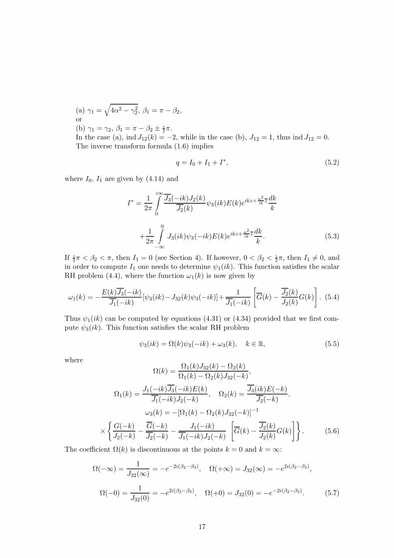
The coefficient Ω(k) is discontinuous at the points k = 0 and k = ∞:

Ω(−∞) =1

J32(∞)= −e−2i(β2−β3), Ω(+∞) = J32(∞) = −e2i(β2−β3),

Ω(−0) =1

J32(0)= −e2i(β2−β3), Ω(+0) = J32(0) = −e−2i(β2−β3). (5.7)

17

We fix the argument of the function Ω(k) as follows

arg Ω(−∞) = π + 2(β3 − β2), arg Ω(+0) = π + 2(β3 − β2). (5.8)

Then

arg Ω(−0) = π + 2(β3 − β2) + ∆−, arg Ω(+∞) = π + 2(β3 − β2) + ∆+, (5.9)

where ∆− (∆+) is the increment of the argument of the function Ω(k) as k passes thenegative (positive) semi-axis. It can be directly verified that Ω(k) = Ω(−k). Therefore∆+ = ∆− = ∆. Comparing (5.7) and (5.9) we find

∆ = 2πκ + 4(β2 − β3), (5.10)

where κ is an integer. The function Ω(k) can be factorised as

Ω(k) =X+(k)

X−(k), k ∈ R, (5.11)

where

X±(k) = kp exp

1

2πi

∞∫

−∞

log Ω(k)

x− kdx

, k ∈ C±, (5.12)

p is an integer defined by the value of the parameter ∆. The analysis of the aboveCauchy integral yields

X(k) ∼ A0kp+ ∆

2π , k → 0,

X(k) ∼ A1kp− ∆

2π , k → ∞, (5.13)

where A0, A1 are constants.We assume

−3π < ∆ < 3π. (5.14)

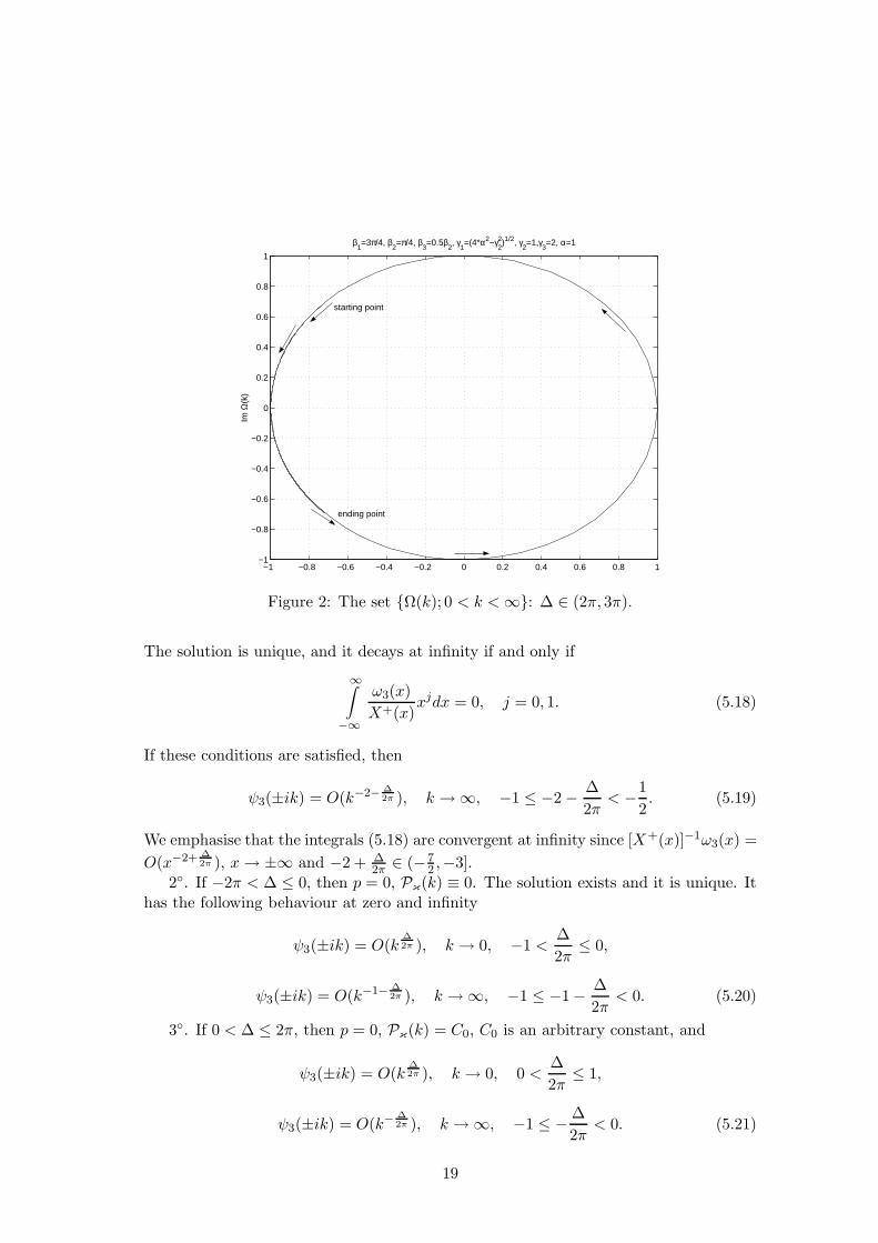
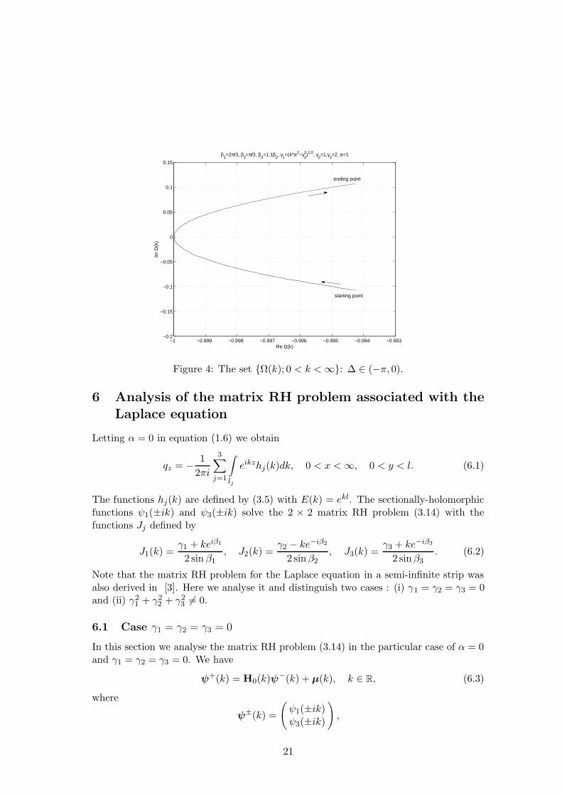
This is consistent with a variety of numerical experiments. Figs 2-5 present graphs ofΩ(k), 0 < k <∞, for α = 1 and some values of the parameters βj , γj . For all these cases(5.14) is valid. Substituting equation (5.11) into (5.5) and using Liouville’s theoremwe find

ψ3(±ik) = X±(k)[χ±(k) + Pκ(k)], k ∈ C± \ R, (5.15)

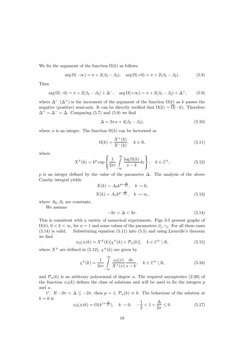
where X± are defined in (5.12), χ±(k) are given by

χ±(k) =1

2πi

∞∫

−∞

ω3(x)

X+(x)

dx

x− k, k ∈ C

± \ R, (5.16)

and Pκ(k) is an arbitrary polynomial of degree κ. The required asymptotics (2.20) ofthe function ψ3(k) defines the class of solutions and will be used to fix the integers pand κ.

1. If −3π < ∆ ≤ −2π, then p = 1, Pκ(k) ≡ 0. The behaviour of the solution atk = 0 is

ψ3(±ik) = O(k1+ ∆2π ), k → 0, −

1

2< 1 +

∆

2π≤ 0. (5.17)

18

−1 −0.8 −0.6 −0.4 −0.2 0 0.2 0.4 0.6 0.8 1−1

−0.8

−0.6

−0.4

−0.2

0

0.2

0.4

0.6

0.8

1

Im Ω

(k)

β1=3π/4, β

2=π/4, β

3=0.5β

2, γ

1=(4*α2−γ

22)1/2, γ

2=1,γ

3=2, α=1

starting point

ending point

Figure 2: The set Ω(k); 0 < k <∞: ∆ ∈ (2π, 3π).

The solution is unique, and it decays at infinity if and only if

∞∫

−∞

ω3(x)

X+(x)xjdx = 0, j = 0, 1. (5.18)

If these conditions are satisfied, then

ψ3(±ik) = O(k−2− ∆2π ), k → ∞, −1 ≤ −2 −

∆

2π< −

1

2. (5.19)

We emphasise that the integrals (5.18) are convergent at infinity since [X+(x)]−1ω3(x) =

O(x−2+ ∆2π ), x→ ±∞ and −2 + ∆

2π ∈ (−72 ,−3].

2. If −2π < ∆ ≤ 0, then p = 0, Pκ(k) ≡ 0. The solution exists and it is unique. Ithas the following behaviour at zero and infinity

ψ3(±ik) = O(k∆2π ), k → 0, −1 <

∆

2π≤ 0,

ψ3(±ik) = O(k−1− ∆2π ), k → ∞, −1 ≤ −1 −

∆

2π< 0. (5.20)

3. If 0 < ∆ ≤ 2π, then p = 0, Pκ(k) = C0, C0 is an arbitrary constant, and

ψ3(±ik) = O(k∆2π ), k → 0, 0 <

∆

2π≤ 1,

ψ3(±ik) = O(k−∆2π ), k → ∞, −1 ≤ −

∆

2π< 0. (5.21)

19

1.1 1.2 1.3 1.4 1.5 1.6 1.7 1.8 1.90

5

10

15

v

b j

1.1 1.2 1.3 1.4 1.5 1.6 1.7 1.8 1.9−20

−15

−10

−5

0

5

v

transonic casea j

−0.8 −0.6 −0.4 −0.2 0 0.2 0.4 0.6 0.8 1−1

−0.8

−0.6

−0.4

−0.2

0

0.2

0.4

0.6

0.8

1

Re Ω(k)

β1=3π/4, β

2=π/4, β

3=1.5β

2, γ

1=(4*α2−γ

22)1/2, γ

2=1,γ

3=2, α=1

Im Ω

(k)

starting point

ending point

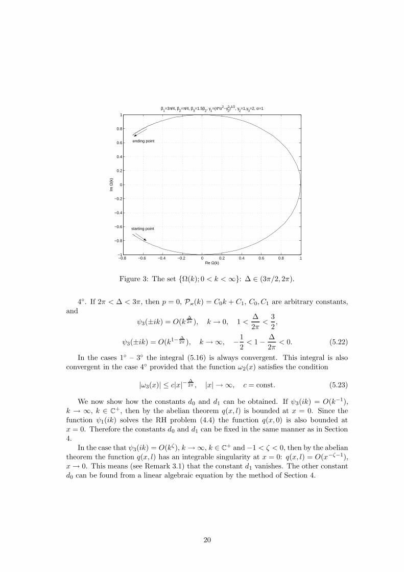
Figure 3: The set Ω(k); 0 < k <∞: ∆ ∈ (3π/2, 2π).

4. If 2π < ∆ < 3π, then p = 0, Pκ(k) = C0k + C1, C0, C1 are arbitrary constants,and

ψ3(±ik) = O(k∆2π ), k → 0, 1 <

∆

2π<

3

2,

ψ3(±ik) = O(k1− ∆2π ), k → ∞, −

1

2< 1 −

∆

2π< 0. (5.22)

In the cases 1 – 3 the integral (5.16) is always convergent. This integral is alsoconvergent in the case 4 provided that the function ω2(x) satisfies the condition

|ω3(x)| ≤ c|x|−∆2π , |x| → ∞, c = const. (5.23)

We now show how the constants d0 and d1 can be obtained. If ψ3(ik) = O(k−1),k → ∞, k ∈ C

+, then by the abelian theorem q(x, l) is bounded at x = 0. Since thefunction ψ1(ik) solves the RH problem (4.4) the function q(x, 0) is also bounded atx = 0. Therefore the constants d0 and d1 can be fixed in the same manner as in Section4.

In the case that ψ3(ik) = O(kζ), k → ∞, k ∈ C+ and −1 < ζ < 0, then by the abelian

theorem the function q(x, l) has an integrable singularity at x = 0: q(x, l) = O(x−ζ−1),x→ 0. This means (see Remark 3.1) that the constant d1 vanishes. The other constantd0 can be found from a linear algebraic equation by the method of Section 4.

20

−1 −0.999 −0.998 −0.997 −0.996 −0.995 −0.994 −0.993−0.2

−0.15

−0.1

−0.05

0

0.05

0.1

0.15

Re Ω(k)

Im Ω

(k)

β1=2π/3, β

2=π/3, β

3=1.1β

2, γ

1=(4*α2−γ

22)1/2, γ

2=1,γ

3=2, α=1

starting point

ending point

Figure 4: The set Ω(k); 0 < k <∞: ∆ ∈ (−π, 0).

6 Analysis of the matrix RH problem associated with the

Laplace equation

Letting α = 0 in equation (1.6) we obtain

qz = −1

2πi

3∑

j=1

∫

lj

eikzhj(k)dk, 0 < x <∞, 0 < y < l. (6.1)

The functions hj(k) are defined by (3.5) with E(k) = ekl. The sectionally-holomorphicfunctions ψ1(±ik) and ψ3(±ik) solve the 2 × 2 matrix RH problem (3.14) with thefunctions Jj defined by

J1(k) =γ1 + keiβ1

2 sin β1, J2(k) =

γ2 − ke−iβ2

2 sinβ2, J3(k) =

γ3 + ke−iβ3

2 sinβ3. (6.2)

Note that the matrix RH problem for the Laplace equation in a semi-infinite strip wasalso derived in [3]. Here we analyse it and distinguish two cases : (i) γ1 = γ2 = γ3 = 0and (ii) γ2

1 + γ22 + γ2

3 6= 0.

6.1 Case γ1 = γ2 = γ3 = 0

In this section we analyse the matrix RH problem (3.14) in the particular case of α = 0and γ1 = γ2 = γ3 = 0. We have

ψ+(k) = H0(k)ψ−(k) + µ(k), k ∈ R, (6.3)

where

ψ±(k) =

(

ψ1(±ik)ψ3(±ik)

)

,

21

−1 −0.8 −0.6 −0.4 −0.2 0 0.2 0.4 0.6 0.8 1−1

−0.8

−0.6

−0.4

−0.2

0

0.2

0.4

0.6

0.8

1

β1=π/4, β

2=3π/4, β

3=1.3β

2, γ

1=(4*α2−γ

22)1/2, γ

2=1,γ

3=2, α=1

Re Ω(k)

Im Ω

(k)

starting point

ending point

Figure 5: The set Ω(k); 0 < k <∞: ∆ ∈ (−3π,−2π).

H0(k) = −1

sinh(kl + iπb)

(

sinh(kl − iπa) i sinβ1

sinβ3sinπ(b− a)

i sinβ3

sin β1sinπ(b+ a) sinh(kl + iπa)

)

,

a =β1 + 2β2 − β3

π, b =

β1 + β3

π, (6.4)

Since 0 < βj < π (j = 1, 2, 3) it follows −1 < a < 3, 0 < b < 2.

6.1.1 Case sinπ(b± a) 6= 0, a = 0.

We construct a closed-form solution of the matrix problem (6.3) assuming that a = 0 andsinπ(b± a) 6= 0, i.e. β2 = 1

2(β3 − β1) and β1 6= −β2 + 1

2πm (m = 1, 2, 3), β3 6= β2 + 1

2πn

(m = 0,±1). In this case the system of functional equations (6.3) decouples to twoseparate scalar RH problems

φ+j (k) = λj(k)φ

−

j (k) + ηj(k), k ∈ R, j = 1, 2. (6.5)

Here

φ±j (k) =1

2

[

ψ1(±ik) + (−1)j−1 sinβ1

sinβ3ψ3(±ik)

]

,

ηj(k) =1

2

[

µ1(k) + (−1)j−1 sinβ1

sinµ3µ3(k)

]

,

λj(k) = −sinhkl + (−1)j−1i sinπb

sinh(kl + πib), j = 1, 2. (6.6)

22

The functions λj(k) can be represented in terms of the Γ-functions as follows

λ1(k) = −Γ(1/2 + b/2 − ik′)Γ(1/2 − b/2 + ik′)

Γ(1/2 + b/2 + ik′)Γ(1/2 − b/2 − ik′),

λ2(k) =Γ(b/2 − ik′)Γ(1 − b/2 + ik′)

Γ(b/2 + ik′)Γ(1 − b/2 − ik′), (6.7)

where k′ = kl2π , b = 2

π (β1 + β2). Next, we factorise the functions λj(k)

λj(k) =X+

j (k)

X−

j (k), k ∈ R, (6.8)

where

X±

1 (k) = ±Γ(1/2 + b/2 ∓ ik′ − δ)

Γ(1/2 − b/2 ∓ ik′ + δ), X±

2 (k) =Γ(b/2 ∓ ik′)

Γ(1 − b/2 ∓ ik′),

δ =

0, 0 < b < 11, 1 < b < 2.

(6.9)

The functions X±

j (k) are analytic and do not vanish in C±. To construct the solution

we need the Cauchy integral

χ±

j (k) =1

2πi

∞∫

−∞

ηj(x)dx

X+j (x)(x− k)

, k ∈ C± \ R. (6.10)

Because of the asymptotics of the functions

X±

1 (k) ∼ ±(∓ik′)b−2δ , X±

2 (k) ∼ (∓ik′)b−1, k → ∞, k ∈ C±, (6.11)

and ηj(x) = O(x−1), x → ∞, the integral (6.10) converges at infinity. By substitutingformula (6.8) into (6.5) and by using (6.10) and Liouville’s theorem we find:

If 0 < β1 + β2 < 12π (0 < b < 1), then

φ±1 (k) = X±

1 (k)χ±

1 (k), k ∈ C±,

φ±2 (k) = X±

2 (k)[C + χ±

2 (k)], k ∈ C±, (6.12)

where C is an arbitrary constant.If 1

2π < β1 + β2 < π (1 < b < 2), then

φ±1 (k) = X±

1 (k)[C + χ±

1 (k)], k ∈ C±,

φ±2 (k) = X±

2 (k)χ±

2 (k), k ∈ C±. (6.13)

The potentials ψ1(±ik) and ψ3(±ik) can be expressed through φ±

1 (k) and φ±2 (k) from(6.6)

ψ1(±ik) = φ±1 (k) + φ±2 (k),

ψ3(±ik) =sinβ3

sinβ1[φ±1 (k) − φ±2 (k)]. (6.14)

23

Using the definition of the functions ψ1(−ik), ψ3(−ik)

ψ1(−ik) =

∞∫

0

e−ikxq(x, 0)dx, ψ3(−ik) =

∞∫

0

e−ikxq(x, l)dx, (6.15)

the asymptotics of the above integrals

ψj(−ik) = O(kb−1−δ), k → ∞, k ∈ C−, (6.16)

and the abelian theorem we estimate the asymptotics of the boundary values of thefunction q(x, y) at the corners of the semi-strip D

q(x, 0) = O(x−b+δ), q(x, l) = O(x−b+δ), x→ 0, −b+ δ ∈ (−1, 0). (6.17)

Thus, d0 = d1 = 0.

6.1.2 Scalar cases

We assume that sinπ(b − a) = sinπ(b + a) = 0, i.e. β1 = −β2 + 12πm (m = 1, 2, 3)

and β3 = β2 + 12πn (n = 0,±1). In this case the matrix H0(k) becomes diagonal and

constant, H0 = diag(−1)m−1, (−1)n−1, and therefore the RH problem (3.14) reducesto

ψ1(ik) = (−1)m−1ψ1(−ik) + µ1(k),

ψ3(ik) = (−1)n−1ψ3(−ik) + µ3(k). (6.18)

Consequently, the solution of the above problems is easily found in terms of the Cauchyintegrals. Clearly, to define the boundary values of the function q(x, y) at y = 0 andy = l one can apply the Fourier transform to (6.18) using formulae (3.8) for α = 0.Thus, for positive x,

q(x, 0) = µ1(x), q(x, l) = µ3(x), (6.19)

where

µj(x) =1

2π

∞∫

−∞

µj(k)e−ikxdk. (6.20)

The functions µj(x) (j = 1, 3) are bounded at x = 0 and therefore the constants d0, d1

can be fixed by the method of Section 4.

6.1.3 Triangular cases

We assume now that sinπ(b − a) = 0 and sinπ(b + a) 6= 0, i.e. β1 6= −β2 + 12πm

(m = 1, 2, 3) and β3 = β2 + 12πn (n = 0,±1). In this case, H0(s) is the following

triangular matrix

H0(s) = (−1)n−1

sin(ikl+πb)sin(ikl−πb) 0

− sin β3 sin 2πbsinβ1 sin(ikl−πb) 1

. (6.21)

24

The problem of interest is the scalar RH problem

ψ1(ik) = (−1)n−1 sinπ(2ik′ + b)

sinπ(2ik′ − b)ψ1(−ik) + µ1(k), k ∈ R, (6.22)

where as before k′ = kl2π . The factorization of the coefficient of the RH problem is given

by

(−1)n−1 sinπ(2ik′ + b)

sinπ(2ik′ − b)=X+(k)

X−(k), k ∈ R, (6.23)

where

X+(k) =Γ(b− δ − 2ik′)

Γ(1 − b+ δ − 2ik′), X−(k) = (−1)n Γ(b− δ + 2ik′)

Γ(1 − b+ δ + 2ik′). (6.24)

The solution to the RH problem (6.22) in the cases 0 < b < 12 and 1 < b < 3

2 involvesan arbitrary constant:

ψ1(±ik) = X±(k)[χ±(k) + C], k ∈ C±. (6.25)

In the cases 12 < b < 1 and 3

2 < b < 2 it is unique:

ψ1(±ik) = X±(k)χ±(k), k ∈ C±, (6.26)

where

χ±(k) =1

2πi

∞∫

−∞

µ1(x)dx

X+(x)(x− k), k ∈ C

± \ R. (6.27)

We note that b = 12 or b = 3

2 imply sinπ(b+ a) = 0. The asymptotics at infinity of thesolution ψ1(±ik) follows from the analysis of formulae (6.24) to (6.27)

ψ1(±ik) = O(k2b−2δ−1−δ′ ), k → ∞, k ∈ C±, (6.28)

where

δ′ =

0, 0 < b < 12 or 1 < b < 3

21, 1

2 < b < 1 or 32 < b < 2

. (6.29)

The abelian theorem yields the asymptotics of the function q(x, 0) as x→ 0

q(x, 0) = O(x2δ+δ′−2b), x→ 0. (6.30)

Clearly, 2δ+δ′−2b ∈ (−1, 0). The above asymptotics implies that d0 = 0. The constantd1 can be found from the corresponding linear algebraic equation following the procedureof Section 4.

The remaining possible case sin 2(β1 + β2) = 0, sin 2(β3 − β2) 6= 0, can be treatedsimilarly.

25

6.2 Case γ21 + γ

22 + γ

33 6= 0: regularisation of the RH problem

We assume that at least one of the constants γj (j = 1, 2, 3) is different than zero. Weaim to regularise the matrix RH problem associated with the Laplace equation in thecase a = 0, β1 6= −β2 + 1

2πm (m = 1, 2, 3) and β3 6= β2 + 1

2πn (n = 0,±1).

According to the Carleman-Vekua method, the corresponding system of Fredholm’sequations can be written explicitly since the dominant part of the matrix H(k), thematrix H0(k), has already been factorised (Section 6.1.1). Using the asymptotics of thematrix H(k) as k → ∞

H(k) = −1

sinh(kl + iπb)

(

sinhkl[1 +O(k−1)] i sinβ1

sinβ3sinπb[1 +O(k−1]

i sinβ3

sinβ1sinπb[1 +O(k−1)] sinh kl[1 +O(k−1)]

)

,

(6.31)we represent the matrix H(k) as follows

H(k) = H0(k) + H(k), H(k) = Hmj(k)m,j=1,2. (6.32)

By following the procedure of Section 6.1 we obtain

φ+j (k) = λj(k)φ

−

j (k) + ηj(k), k ∈ R, j = 1, 2, (6.33)

where2ηj(k) = µ1(k) + H11(k)ψ1(−ik) + H12(k)ψ3(−ik)

−(−1)j sinβ1

sinβ3[µ3(k) + H21(k)ψ1(−ik) + H22(k)ψ3(−ik)]. (6.34)

Using the solution of Section 6.1 yields another representation of the RH problem. Forexample, in the case 0 < b < 1 we have

ψ1(−ik) =X−

1 (k)

2πi

∞∫

−∞

η1(ζ)dζ

X+1 (ζ)(ζ − k)

+X−

2 (k)

1

2πi

∞∫

−∞

η2(ζ)dζ

X+2 (ζ)(ζ − k)

+ C

.

ψ3(−ik) =sinβ3

sinβ1

X−

1 (k)

2πi

∞∫

−∞

η1(ζ)dζ

X+1 (ζ)(ζ − k)

−X−

2 (k)

1

2πi

∞∫

−∞

η2(ζ)dζ

X+2 (ζ)(ζ − k)

+ C

.

(6.35)Substituting (6.34) into (6.35) and then taking the limit as k = kR − i0, we find asystem of the Fredholm integral equations [7]. Alternatively, we can apply the inverseFourier transform to the above equations, change the order of integration and make thesubstitution πx = −l log ξ,

r(ξ) +

1∫

0

R(ξ, τ)r(τ)dτ = p(ξ), 0 < ξ < 1, (6.36)

where

r1(ξ) = q

(

l

πlog

1

ξ, 0

)

, r2(ξ) = q

(

l

πlog

1

ξ, l

)

, (6.37)

Rmj(ξ, τ), the elements of the matrix R(ξ, τ), are Fredholm’s kernels. They are repre-sented by double quadratures and can be evaluated by the residue theorem.

26

7 Conclusions

In this paper we have studied the modified Helmholtz equation (1.2) in a semi-stripwith the Poincare type boundary conditions (1.1). On each side of the semi-strip, theboundary conditions involve two real constants βj , γj and a real-valued function gj ,j = 1, 2, 3.

Using the method reviewed in [1] it is straightforward to reduce the above boundary-value problem to a 2×2 matrix RH problem for the two sectionally holomorphic functionsψ1(±ik) and ψ3(±ik), k ∈ C

±. The jump matrix H(k) of the associated RH problem(3.14) on the real k-axis is uniquely defined in terms of the scalar functions Jj(k),j = 1, 2, 3, which are in turn defined in terms of the constant α entering in the modifiedHelmholtz equation, and in terms of the constants βj , γj, j = 1, 2, 3.

A crucial role in the investigation of the above RH problem is played by the products

J12(k)J12(−k), J32(k)J32(−k), (7.1)

where J12(k) and J32(k) are defined in terms of Jj(k) j = 1, 2, 3, by equation (4.1).There exist the following three particular cases:

I. J12(k)J12(−k) = 1, J32(k)J32(−k) = 1.In this case the basic RH problem reduces to two separate scalar RH problems, one

for the sectionally holomorphic function ψ1(±ik) and one for ψ3(±ik). Each of these RHproblems can be solved in closed form; the solutions depend on the particular relations

between βj and γj. (a) If γ1 =√

4α2 − γ22 , β1 = π − β2, then the solution ψ1(±ik)

exists under the conditions (4.33) and it is given by equation (4.31). (b) If γ1 = γ2,β1 = 1

2π − β2, ψ1(±ik) is given by equation (4.34). Similar considerations are valid for

ψ3(±ik).The solution q(x, y) of the modified Helmholtz equation also depends on the particu-

lar relations between βj and γj: 1. If these parameters satisfy (4.18) or (4.19) or (4.20),then q = I0 + I2, where the integrals I0 and I2 depend only on the given boundary con-ditions, see equations (4.14) (in these cases ψ1(±ik) and ψ3(±ik) do not contribute tothe solution). 2. If the parameters satisfy (4.22), then q = I0 +I1 +I2, where I1 depends

on ψ1(ik(2)1 ) and k

(2)1 is known , see equation (4.16). 3. If the parameters satisfy (4.24),

then q = I0 + I2 + I3, where I3 depends on ψ3(ik(2)2 ), and k

(2)2 is known, see equation

(4.16).

Having constructing ψ1(ik), ψ3(ik), the values ψ1(ik(2)1 ) and ψ3(ik

(2)2 ) follow.

II. J12(k)J12(−k) = 1, J32(k)J32(−k) 6= 1.In this case the basic RH problem is triangular. It can be reduced to the scalar

RH problem (5.5) for the sectionally holomorphic function ψ3(±ik) and to a scalar RHproblem for ψ1(±ik) whose jump depends on ψ3(±ik). Thus, after determining ψ3(±ik),ψ1(±ik) can be computed in closed form by solving a scalar RH problem similar to theone mentioned in I above. The scalar RH problem for ψ3(±ik), whose coefficient isdiscontinuous at k = 0 and k = ∞, is solved by equations (5.15).

The solution q is given by q = I0 + I1 + I∗, where I1 depends of ψ1(±ik) (see (4.14))and I∗ depends on ψ3(±ik) (see (5.3).

III. J12(k)J12(−k) 6= 1, J32(k)J32(−k) = 1.

27

This case is similar to II above.We have also analysed the basic RH problem associated with the Laplace equation

(α = 0). We have shown that if β2 = 12(β3 − β2) and γ1 = γ2 = γ3, then the corre-

sponding matrix RH problem can be solved in closed form. If however at least one ofthe parameters γj (j = 1, 2, 3) is not equal to zero then a closed-form solution does notappear feasible. In this case the RH problem has been regularised, i.e. reduced to asystem of two Fredholm integral equations.

Remark 7.1. We recall that the spectral functions (2.13) depend on the three un-known functions ψ1(ik), ψ2(ik), ψ3(ik). The basic RH problem is a consequence ofeliminating ψ2(ik). It was shown in [3] that it is also possible to solve the Laplaceequation in the semi-strip by eliminating either ψ1(ik) or ψ3(ik) instead of ψ2(k). Thisalternative approach has certain advantages since ψ2(k) is an entire function (see [6] forthe analogous problem for the evolution equation). The implementation of this approachto the modified Helmholtz equation remains open.

References

[1] A.S. Fokas. On the integrability of linear and nonlinear PDEs. J. Math. Phys. 41

(2000), 4188-4237.

[2] A.S Fokas. Two dimensional linear PDEs in a convex polygon. Proc. R. Soc. Lond.

A 457 (2001), 371-393.

[3] A.S Fokas and A. Kapaev. A transform method for the Laplace equation in apolygon. (2002), preprint.

[4] A.S Fokas and M.Zyskin. The fundamental differential form and boundary valueproblems. Quart. J. Mech. appl. Math. 55 (2002), 457-479.

[5] F.D. Gakhov. Boundary Value Problems. (Pergamon Press, Oxford, 1966).

[6] B. Pelloni. Well-posedness for two-point boundary value problems. Math. Proc.

Cambridge Phil. Soc. (2002), to appear.

[7] X. Zhou. The Riemann-Hilbert problem and inverse scattering. SIAM J. Math.

Anal. 20 (1989), 966-986.

28