1
The Modified Optimal Velocity Model:
Stability Analyses and Design Guidelines
Gopal Krishna Kamath∗, Krishna Jagannathan and Gaurav Raina
Department of Electrical Engineering, Indian Institute of Technology Madras, Chennai 600 036, India
Email: ee12d033, krishnaj, [email protected]
Abstract
Reaction delays are important in determining the qualitative dynamical properties of a platoon of vehicles traveling
on a straight road. In this paper, we investigate the impact of delayed feedback on the dynamics of the Modified
Optimal Velocity Model (MOVM). Specifically, we analyze the MOVM in three regimes – no delay, small delay
and arbitrary delay. In the absence of reaction delays, we show that the MOVM is locally stable. For small delays,
we then derive a sufficient condition for the MOVM to be locally stable. Next, for an arbitrary delay, we derive the
necessary and sufficient condition for the local stability of the MOVM. We show that the traffic flow transits from
the locally stable to the locally unstable regime via a Hopf bifurcation. We also derive the necessary and sufficient
condition for non-oscillatory convergence and characterize the rate of convergence of the MOVM. These conditions
help ensure smooth traffic flow, good ride quality and quick equilibration to the uniform flow. Further, since a Hopf
bifurcation results in the emergence of limit cycles, we provide an analytical framework to characterize the type of the
Hopf bifurcation and the asymptotic orbital stability of the resulting non-linear oscillations. Finally, we corroborate
our analyses using stability charts, bifurcation diagrams, numerical computations and simulations conducted using
MATLAB.
Index Terms
Transportation networks, car-following models, time delays, stability, convergence, Hopf bifurcation.
I. INTRODUCTION
Intelligent transportation systems constitute a substantial theme of discussion on futuristic smart cities. In this
context, self-driven vehicles are a prospective solution to address traffic issues such as resource utilization and
commute delays; see [1, Section 5.2], [2]–[4] and references therein. To ensure that these objectives are met, in
addition to ensuring human safety, the design of control algorithms for these vehicles becomes important. To that
end, it is imperative to have an in-depth understanding of human behavior and vehicular dynamics. This has led to
the development and study of a class of dynamical models known as the car-following models [5]–[10].
∗ Corresponding author
A part of this work appeared in Proceedings of the 53rd Annual Allerton Conference on Communication, Control and Computing, pp.
538-545, 2015. DOI: 10.1109/ALLERTON.2015.7447051
2
Feedback delays play an important role in determining the qualitative behavior of dynamical systems [11]. In
particular, these delays are known to destabilize the system and induce oscillatory behavior [10], [12]. In the
context of human-driven vehicles, predominant components of the reaction delay are psychological and mechanical
in nature [12]. In contrast, delays in self-driven vehicles arise due to sensing, communication, signal processing
and actuation, and are envisioned to be smaller than human reaction delays [13].
In this paper, we investigate the impact of delayed feedback on the qualitative dynamical properties of a platoon
of vehicles traveling on a straight road. Specifically, we consider each vehicle’s dynamics to be modeled by the
Modified Optimal Velocity Model (MOVM) [10]. Motivated by the wide range of values assumed by reaction
delays in various scenarios, we analyze the MOVM in three regimes; namely, (i) no delay, (ii) small delay and
(iii) arbitrary delay. In the absence of delays, we show that the MOVM is locally stable. When the delays are
rather small, as in the case of self-driven vehicles, we derive a sufficient condition for the local stability of the
MOVM using a suitable approximation. For the arbitrary-delay regime, we analytically characterize the region of
local stability for the MOVM.
In the context of transportation networks, two additional properties are of practical importance; namely, ride
quality (lack of jerky vehicular motion) and the time taken by the platoon to attain the desired equilibrium when
perturbed. Mathematically, these translate to studying the non-oscillatory property of the MOVM’s solutions and
the rate of their convergence to the desired equilibrium. In this paper, we also characterize these properties for the
MOVM.
In the context of human-driven vehicles, model parameters generally correspond to human behavior, and hence
cannot be “tuned” or “controlled.” However, our work enhances phenomenological insight into the emergence and
evolution of traffic congestion. For example, a peculiar phenomenon known as the “phantom jam” is observed on
highways [7], [8]. Therein, a congestion wave emerges seemingly out of nowhere and propagates up the highway
from the point of its origin. Such an oscillatory behavior in the traffic flow has typically been attributed to a
change in the driver’s sensitivity, such as a sudden deceleration; for details, see [7], [8]. In general, feedback delays
are known to induce oscillations in state variables of dynamical systems [10], [12]. Since the MOVM explicitly
incorporates feedback delays, and relative velocities and headways constitute state variables of the MOVM, our
work provides a theoretical basis for understanding the emergence and evolution of oscillatory phenomena such as
“phantom jams.” In particular, our work serves to highlight the possible role of reaction delays in the emergence
of oscillatory phenomena in traffic flows. More generally, our results reveal an important observation: the traffic
flow may transit into instability due to an appropriate variation in any subset of model parameters. To capture this
complex dependence of stability on various parameters, we introduce an exogenous, non-dimensional parameter in
our dynamical model. We then analyze the behavior of the resulting system as the exogenous parameter is pushed
just beyond the stability boundary. We show that non-linear oscillations, termed limit cycles, emerge in the traffic
flow due to a Hopf bifurcation.
In the context of self-driven vehicles, reaction delays are expected to be smaller than their human counterparts [13].
Hence, it would be realistically possible to achieve smaller equilibrium headways [1, Section 5.2]. This would, in
turn, vastly improve resource utilization without compromising safety [3]. In this paper, based on our theoretical
3
analyses, we provide some design guidelines to appropriately tune the parameters of the so-called “upper longitudinal
control algorithm” [1, Section 5.2]. Mathematically, our analytical findings highlight the quantitative impact of
delayed feedback on the design of control algorithms for self-driven vehicles. Specifically, our design guidelines
take into consideration various aspects of the longitudinal control algorithm such as stability, good ride quality
and fast convergence of the traffic to the uniform flow. In the event that the traffic flow does lose stability, our
design guidelines help tune the model parameters with an aim of reducing the amplitude and angular velocity of
the resultant limit cycles.
A. Related work on car-following models
The motivation for our paper comes from the key idea behind the Optimal Velocity Model (OVM) proposed
by Bando et al. in [14] for a platoon of vehicles on a circular loop. However, the model considered therein was
devoid of reaction delays. Thus, a new model was proposed in [6] to account for the drivers’ delays. Therein,
the authors also claimed that these delays were not central to capturing the dynamics of the system. In response,
Davis showed via numerical computations that reaction delays indeed play an important part in determining the
qualitative behavior of the OVM [15]. This led to a further modification to the OVM in [16]. However, this too
did not account for the delay arising due to a vehicle’s own velocity. It was shown in [17] that the OVM without
delays loses local stability via a Hopf bifurcation. For the OVM with delays, [18] performed an initial numerical
study of the bifurcation phenomenon before supplying an analytical proof in [9].
While a control-theoretic treatment of car-following models has been widely studied (see [19]–[21] and references
therein), the thematic issue on “Traffic jams: dynamics and control” [22] highlights the growing interest in a
synergized control-theoretic and dynamical systems viewpoint of transportation networks. A recent exposition of
linear stability analysis in the context of car-following models can be found in [23].
From a vehicular dynamics perspective, most upper longitudinal controllers in the literature assume the lower
controller’s dynamics to be well modeled by a first-order control system, in order to capture the delay lag [1, Section
5.3]. The upper longitudinal controllers are then designed to maintain either constant velocity, spacing or time gap;
for details, see [24] and the references therein. Specifically, it was shown in [24] that synchronization with the
lead vehicle is possible by using information only from the vehicle directly ahead. This reduces implementation
complexity, and does not mandate vehicles to be installed with communication devices.
However, in the context of autonomous vehicles, communication systems are required to exchange various system
states required for the control action. This information is used either for distributed control [24] or coordinated
control [25] of vehicles. Formation control [26], [27] and platoon stabilities [28] have also been studied considering
information flow among the vehicles. However, these works do not consider the effect of delays in relaying the
required information. In contrast, when latency increases due to randomness in the communication environment,
strategies have been developed to make use of only on-board sensors with minimal degradation in performance [29].
For an extensive review, see [20]. Usage of communication systems is also known to mitigate phantom jams [30].
It may be noted that, for our scenario of straight road with a single lane, the formation control problem subsumes
4
the problem of stabilizing a platoon. Thus, our work can also be thought of as a formation control problem in the
presence of reaction delays and using only on-board sensors.
At a microscopic level, Chen et al. proposed a behavioral car-following model based on empirical data that
captures phantom jams [31]. Therein, the authors showed statistical correlation in drivers’ behavior before and
during traffic oscillations. However, no suggestions to avoid phantom jams were offered. To that end, Nishi et al.
developed a framework for “jam-absorbing” driving in [32]. A “jam-absorbing vehicle” appropriately varies its
headway with the aim of mitigating phantom jams. This work was extended by Taniguchi et al. [33] to include
car-following behavior. Therein, the authors also numerically constructed the region in parameter space that avoids
formation of secondary jams.
In the context of platoon stability, it has been shown that well-placed, communicating autonomous vehicles may
be used to stabilize platoons of human-driven vehicles [34]. More generally, the platooning problem has been
studied as a consensus problem with delays [35]. Such an approach aids the design of coupling protocols between
interacting agents (in this context, vehicles). In contrast, we provide design guidelines to appropriately choose
protocol parameters, for a given coupling protocol. Additionally, the effect of communication delays has been been
studied in the literature, both when the delays are deterministic [36] and random [37]. It may be noted that, our
work differs from these at a fundamental level; these models assume vehicles to be traversing a circular loop, thus
yielding a periodic boundary condition. In contrast, our work studies the effect of (deterministic) reaction delays
on the qualitative dynamics of a platoon of vehicles using the MOVM on a straight road. Further, in addition to
characterizing the region for local stability, we study two practically relevant properties – non-oscillatory convergence
and the rate of convergence. More importantly, our analysis goes beyond that of the linearized system by making use
of bifurcation theory to take into account non-linear terms. For a treatment of bifurcations in non-delayed systems,
the reader is referred to the classical text by Guckenheimer and Holmes [38]; for Hopf bifurcations in systems with
time delays, the reader may refer to the excellent texts by Hassard et al. [39] or Marsden and McCracken [40].
B. Our contributions
Our contributions are as follows.
(1) We derive a variant of the OVM for an infinitely-long road – called the MOVM – and analyze it in three
regimes; namely, (i) no delay, (ii) small delay and (iii) arbitrary delay. We prove that the ideal case of
instantaneously-reacting drivers is locally stable for all practically significant parameter values. We then derive
a stability condition for the small-delay regime by conducting a linearization on the time variable.
(2) For the case of an arbitrary delay, we derive the necessary and sufficient condition for the local stability of
the MOVM. We then prove that, upon violation of this condition, the MOVM loses local stability via a Hopf
bifurcation.
(3) We provide an analytical framework to characterize the type of the Hopf bifurcation and the asymptotic orbital
stability of the emergent limit cycles using Poincare normal forms and the center manifold theory.
(4) In the case of human-driven vehicles, our work enhances phenomenological insight into the emergence and
evolution of traffic congestion. For example, the Hopf bifurcation analysis provides a mathematical framework
5
to offer a possible explanation for the observed “phantom jams” [10]. In the case of self-driven vehicles, our
work offers suggestions for their design guidelines.
(5) We derive a necessary and sufficient condition for non-oscillatory convergence of the MOVM. This is useful in
the context of a transportation network since oscillations lead to jerky vehicular movements, thereby degrading
ride quality and possibly causing collisions.
(6) We characterize the rate of convergence of the MOVM, thereby gaining insight into the time required for
the platoon to equilibrate, when perturbed. Such perturbations occur, for instance, when a vehicle departs
from a platoon. Therein, we also bring forth the trade-off between the rate of convergence and non-oscillatory
convergence of the MOVM.
(7) We corroborate the analytical results with the aid of stability charts, bifurcation diagrams, numerical compu-
tations and simulations performed using MATLAB.
The remainder of this paper is organized as follows. In Section II, we summarize the OVM and derive the
MOVM. In Sections III, IV and V, we characterize the stable regions for the MOVM in no-delay, small-delay
and arbitrary-delay regimes respectively. We then derive the necessary and sufficient condition for non-oscillatory
convergence of the MOVM in Section VI, and characterize its rate of convergence in Section VII. In Section VIII,
we present the local Hopf bifurcation analysis for the MOVM. In Section IX, we corroborate our analyses using
MATLAB simulations before concluding the paper in Section X.
II. MODELS
In this section, we first provide an overview of the setting of our work. We then briefly explain the OVM, before
ending the section by deriving the MOVM.
A. The setting
We consider N + 1 idealistic vehicles (with 0 length) traveling on an infinitely long, single-lane road with no
overtaking. The lead vehicle is indexed with 0, the vehicle following it with 1, and so on. The acceleration of each
vehicle is updated based on a combination of its position, velocity and acceleration as well as those corresponding
to the vehicle directly ahead. We use xi(t), xi(t) and xi(t) to denote the position, velocity and acceleration of the
vehicle indexed i at time t respectively. We also assume that the lead vehicle’s acceleration and velocity profiles
are known. Specifically, we only consider leader profiles that converge to x0 = 0 and 0 < x0 < ∞ in finite time;
that is, there exists T0 < ∞ such that x0(t) = 0, x0(t) = x0 > 0, ∀ t ≥ T0. We also use the terms “driver” and
“vehicle” interchangeably throughout. Further, we make use of SI units throughout.
B. The Optimal Velocity Model (OVM)
The OVM, proposed by Bando et al. in [14], is based on the key idea that each vehicle in a platoon tries to attain
an “optimal” velocity, which a function of its headway. Hence, each vehicle updates its acceleration proportional
6
to the difference between this optimal velocity and its own velocity. This was modified in [6] to account for the
reaction delay. For N vehicles traveling on a circular loop of length L units, the dynamics is captured by [6]
x1(t) = a (V (xN (t− τ) − x1(t− τ)) − x1(t− τ)) ,
xi(t) = a (V (xi−1(t− τ)− xi(t− τ)) − xi(t− τ)) , (1)
for i ∈ 2, · · · , N. Here, a > 0 is the drivers’ sensitivity coefficient, τ is the common reaction delay and
V : R+ → R+ is called the Optimal Velocity Function (OVF). As pointed out in [41], an OVF satisfies:
(i) Monotonic increase,
(ii) Bounded above, and,
(iii) Continuous differentiability.
Let V max = limy→∞
V (y). The limit exists as a consequence of (i) and (ii) above. Also, (iii) ensures that an OVF
will be invertible.
C. The Modified Optimal Velocity Model (MOVM)
Next, we derive a version of the OVM for the infinite highway setting. To that end, we begin by re-writing
system (1) as
x1(t) = a (V (x0(t− τ1)− x1(t− τ1))− x1(t− τ1)) ,
xi(t) = a (V (xi−1(t− τi)− xi(t− τi))− xi(t− τi)) , (2)
where x0(t) is the position of the lead vehicle at time t. To capture reality better, we have accounted for heterogeneity
in reaction delays. Notice that, in contrast to (1), system (2) no longer possesses the circular structure resulting
from the periodic boundary condition. Indeed, the second vehicle (with index 1) now follows the lead vehicle rather
than the vehicle with index N. Further, each vehicle requires external information from the vehicle preceding it
only. Hence, on a technological level, on-board sensors suffice to implement our strategy.
From (2), it may be noted that xi(t) → ∞ as t → ∞ for each i. To apply tools from non-linear dynamics, we
require bounded state variables. To that end, we use the change of variables yi(t) = xi−1(t) − xi(t) and vi(t) =
yi(t) = xi−1(t)− xi(t). Here, yi(t) and vi(t) represent the relative distance (headway) and relative velocity between
the vehicles i and i− 1 at time t respectively. Substituting these in (2), we obtain the following system after some
algebraic manipulations
v1(t) = x0(t) + a (x0(t− τ1)− V (y1(t− τ1))− v1(t− τ1)) ,
vk(t) = a (V (yk−1(t− τk−1))− V (yk(t− τk))− vk(t− τk)) ,
yi(t) = vi(t), (3)
for i ∈ 1, 2, · · · , N and for k ∈ 2, 3, · · · , N. We refer to system (3) as the Modified Optimal Velocity Model
(MOVM). We emphasize that, given the absolute variables xiNi=1, the relative variables yiNi=1 are uniquely
determined, and vice versa (when the initial positions are known). Hence, systems (2) and (3) are equivalent, i.e.,
they are representations of the same system in different variables.
7
The MOVM is described by a system of Delay Differential Equations (DDEs). Since such systems are hard to
analyze, we obtain conditions for their local stability by analyzing them in the neighborhood of their equilibria. Such
an analysis technique is called local stability analysis. To obtain the equilibrium for the MOVM, we first equate the
Right Hand Sides (RHSs) corresponding to yi(t) to zero, thus yielding v∗i = 0 for each i. Next, we equate the RHSs
corresponding to vk(t) to zero, for k ∈ 2, 3, · · · , N. Using the equilibria for the relative velocities, we obtain
V (y∗i ) = V (y∗j ), ∀ i, j. Equating the RHS of the very first differential equation to zero, we obtain V (y∗1) = x0.
Combining these, and using the properties of the OVF, we obtain y∗i = V −1(x0) for each i. Therefore, v∗i = 0,
y∗i = V −1(x0), i = 1, 2, · · · , N represents the unique equilibrium of the MOVM. Therefore, to linearize (3) about
this equilibrium, we first consider a small perturbation ui(t) about the equilibrium of the relative spacing pertaining
to vehicle indexed i. That is, ui(t) = yi(t) - y∗i . Next, we consider the Taylor’s series expansion of ui(t), and set
the leader’s profile to zero, to obtain the linearized model, given by
v1(t) = − du1(t− τ1)− av1(t− τ1),
vk(t) = duk−1(t− τk−1)− duk(t− τk)− avk(t− τk),
ui(t) = vi(t), (4)
for i ∈ 1, 2, · · · , N and for k ∈ 2, 3, · · · , N. Here, d = aV′
(V −1(x0)) is the equilibrium coefficient, where the
prime indicates differentiation with respect to a state variable. Henceforth, we denote d = V′
(V −1(x0)). Therefore,
d = ad.
The MOVM is completely specified by the relative velocities vi’s and the headways yi’s. Therefore, the state of
the MOVM at time “t” is given by S(t) = [v1(t) v2(t) · · · vN (t) u1(t) u2(t) · · ·uN (t)]T ∈ R2N . Thus, system (4)
can be succinctly written in matrix form as
S(t) =
N∑
k=0
AkS(t− τk). (5)
This is the evolution equation of the MOVM in the standard state-space representation. Here, τ0 is introduced for
notational brevity and set to zero. Also, the matrices Ak ∈ R2N×2N for each k are the dynamics matrices, which
capture the dependence of the derivative on the state variable delayed by the kth reaction delay. For instance, when
N = 2, the evolution equations are
v1(t) = − du1(t− τ1)− av1(t− τ1),
v2(t) = du1(t− τ1)− du2(t− τ2)− av2(t− τ2),
y1(t) = v1(t),
y2(t) = v2(t).
8
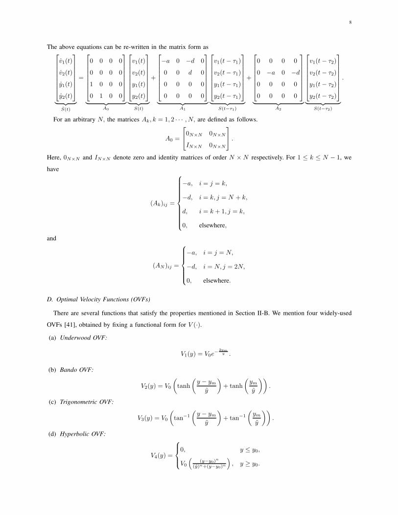
The above equations can be re-written in the matrix form as
v1(t)
v2(t)
y1(t)
y2(t)
︸ ︷︷ ︸
S(t)
=
0 0 0 0
0 0 0 0
1 0 0 0
0 1 0 0
︸ ︷︷ ︸
A0
v1(t)
v2(t)
y1(t)
y2(t)
︸ ︷︷ ︸
S(t)
+
−a 0 −d 0
0 0 d 0
0 0 0 0
0 0 0 0
︸ ︷︷ ︸
A1
v1(t− τ1)
v2(t− τ1)
y1(t− τ1)
y2(t− τ1)
︸ ︷︷ ︸
S(t−τ1)
+
0 0 0 0
0 −a 0 −d0 0 0 0
0 0 0 0
︸ ︷︷ ︸
A2
v1(t− τ2)
v2(t− τ2)
y1(t− τ2)
y2(t− τ2)
︸ ︷︷ ︸
S(t−τ2)
.
For an arbitrary N, the matrices Ak, k = 1, 2 · · · , N, are defined as follows.
A0 =
0N×N 0N×N
IN×N 0N×N
.
Here, 0N×N and IN×N denote zero and identity matrices of order N ×N respectively. For 1 ≤ k ≤ N − 1, we
have
(Ak)ij =
−a, i = j = k,
−d, i = k, j = N + k,
d, i = k + 1, j = k,
0, elsewhere,
and
(AN )ij =
−a, i = j = N,
−d, i = N, j = 2N,
0, elsewhere.
D. Optimal Velocity Functions (OVFs)
There are several functions that satisfy the properties mentioned in Section II-B. We mention four widely-used
OVFs [41], obtained by fixing a functional form for V (·).
(a) Underwood OVF:
V1(y) = V0e−
2ymy .
(b) Bando OVF:
V2(y) = V0
(
tanh
(y − ymy
)
+ tanh
(ymy
))
.
(c) Trigonometric OVF:
V3(y) = V0
(
tan−1
(y − ymy
)
+ tan−1
(ymy
))
.
(d) Hyperbolic OVF:
V4(y) =
0, y ≤ y0,
V0
((y−y0)
n
(y)n+(y−y0)n
)
, y ≥ y0.
9
Here, V0, y0, ym, y and n are model parameters.
As captured by [42, Figure 1], the aforementioned OVFs behave similarly with varying headway. The following
are noteworthy: (i) The values attained by these OVFs, in the vicinity of the equilibrium, are almost the same,
(ii) their slopes, evaluated at the equilibrium, are different. The linearized version of the MOVM, captured by
system (5), brings forth the dependence on the slope via the variable d, and (iii) we make use of the Bando OVF
throughout this paper, except in Section VIII. Therein, we consider both the Bando OVF and the Underwood OVF,
consistent with [10].
We now proceed to understand the dynamical behavior of a platoon of cars running the MOVM.
III. THE NO-DELAY REGIME
We first consider the idealistic case of instantaneously-reacting drivers. This results in zero reactions delays.
Therefore, the model described by system (5) boils down to the following system of Ordinary Differential Equations
(ODEs):
S(t) =
(N∑
k=0
Ak
)
S(t). (6)
We denote by A, the sum of matrices Ak, which is known as the dynamics matrix. To characterize the stability
of system (6), we require the eigenvalues of A to be negative [43, Theorem 5.1.1]. To that end, we compute its
characteristic function as
f(λ) = det(λI2N×2N −A) = det
(λ+ a)IN×N D
IN×N λIN×N
= 0,
where D is derived from the dynamics matrix A. The diagonal entries of D are all d, while its sub-diagonal entries
are −d. Further, the diagonal matrices of the above block matrix are invertible, and the off-diagonal matrices
commute with each other. Hence, from [44, Theorem 3], the characteristic equation can be simplified to (λ2+aλ+
d)N = 0, which holds true if and only if
λ2 + aλ+ d = 0. (7)
Solving the above quadratic, we notice that the poles corresponding to system (6) will be negative if a > 0
and d = V′
(V −1(x0)) > 0. We note that, from physical constraints, a > 0. Also, since V (·) is an OVF, it
is monotonically increasing. Therefore, d > 0. Hence, for all physically relevant values of the parameters, the
corresponding poles will lie in the open left-half of the Argand plane. Thus, the MOVM is locally stable for all
physically relevant values of the parameters, in the absence of delays.
IV. THE SMALL-DELAY REGIME
Having studied the MOVM in the absence of reaction delays, we now analyze it in the small-delay regime. A
way to obtain insight for the case of small delays is to conduct a linearization on time. This would yield a system
of ODEs, which serves as an approximation to the original infinite-dimensional system (5), valid for small delays.
10
We derive the criterion for such a system of ODEs to be stable, thereby emphasizing the design trade-off inherent
among various system parameters and the reaction delay.
We begin by applying the Taylor’s series approximation to the time-delayed state variables thus: vi(t − τi) ≈vi(t) − τivi(t), and ui(t − τi) ≈ ui(t) − τiui(t). Using this approximation for terms in (4), substituting vi(t) for
ui(t) and re-arranging the resulting equations, we obtain the matrix equation
BS(t) = AS(t). (8)
where the matrix A is the dynamics matrix, as defined in Section III, and B is a block matrix of the form
B =
Bs 0N×N
0N×N IN×N ,
,
where
(Bs)ij =
1− aτi, i = j,
0, elsewhere.
We note that, since Bs is a diagonal matrix, so is B. Also, B is invertible if and only if aτi 6= 1, for each i. Thus,
when aτi 6= 1, for each i, we define C = B−1A, which is of the form
C =
Cs Cc
IN×N 0N×N ,
,
where
(Cs)ij =
−a+dτi1−aτi
, i = j,
−dτj1−aτi
, j = i− 1,
0, elsewhere,
and
(Cc)ij =
−d1−aτi
, i = j,
d1−aτi
, j = i− 1,
0, elsewhere.
For system (8) to be stable, the real part of eigenvalues of C must be negative [43, Theorem 5.1.1]. To that end,
we compute its characteristic function as
f(λ) = det(λI2N×2N − C) = det
λIN×N − Cs −Cc
−IN×N λIN×N
= 0.
The diagonal matrices of the aforementioned block matrix are invertible, and the matrices in the second row therein
commute with each other. Hence, the characteristic equation simplifies to [44, Theorem 3]
f(λ) = det(
λ(λIN×N − Cs)− Cc
)
= 0.
11
On further simplification, this yields
f(λ) =N∏
i=1
((1 − aτi)λ
2 + (a− dτi)λ+ d)= 0.
For multiple terms in the above product to equal zero, their respective reaction delays must be equal. Such a
possibility is not realistic, hence we ignore it. Therefore, for some i ∈ 1, 2, · · · , N, we have
(1− aτi)λ2 + (a− dτi)λ+ d = 0.
The roots of this quadratic equation are given by
λ1,2 =−(a− dτi)±
√
(a− dτi)2 − 4d(1− aτi)
2(1− aτi).
We now consider the following (exhaustive) cases.
(1) Let aτi > 1. Since d > 0, it follows that 4d(1−aτi) < 0. Then, the eigenvalues are real. Further, one of these
eigenvalues will be positive and the other negative. Hence, we require aτi < 1 for system (8) to be stable.
(2) Let (a − dτi)2 ≥ 4d(1 − aτi). Then, the eigenvalues are real. They are negative if and only if a − dτi > 0,
i.e., dτi < 1. Hence, we require dτi < 1 for system (8) to be stable.
(3) Let (a − dτi)2 < 4d(1 − aτi). Then, the eigenvalues are complex. The real part of the eigenvalues will be
negative if and only if a− dτi > 0, i.e., dτi < 1. Hence, we require dτi < 1 for system (8) to be stable.
From the above cases, it is clear that system (8) is stable if and only if
max(a, d)τi < 1, (9)
for each i ∈ 1, 2, · · · , N. Recall that we obtained system (8) by truncating the Taylor’s series to first order.
Hence, (9) is a sufficient condition for the local stability of the MOVM described by system (3), valid for small
values of the reaction delay.
V. THE ARBITRARY-DELAY REGIME
Having studied system (3) in the no-delay and the small-delay regimes, in this section, we focus on the arbitrary-
delay regime. We first derive the necessary and sufficient condition for the local stability of the MOVM. We then
show that, upon violation of this condition, the corresponding traffic flow transits via a Hopf bifurcation to the
locally unstable regime.
A. Transversality condition
Hopf bifurcation is a phenomenon wherein, on appropriate variation of system parameters, a dynamical system
either loses or regains stability because of a pair of conjugate eigenvalues crossing the imaginary axis in the Argand
plane [11, Chapter 11, Theorem 1.1]. Mathematically, Hopf bifurcation analysis is a rigorous way of proving the
emergence of limit cycles (isolated closed trajectory in state space) in non-linear dynamical systems.
To determine if system (3) undergoes a stability loss via a Hopf bifurcation, we follow [45] and introduce an
exogenous, non-dimensional parameter κ > 0. A general system of DDEs
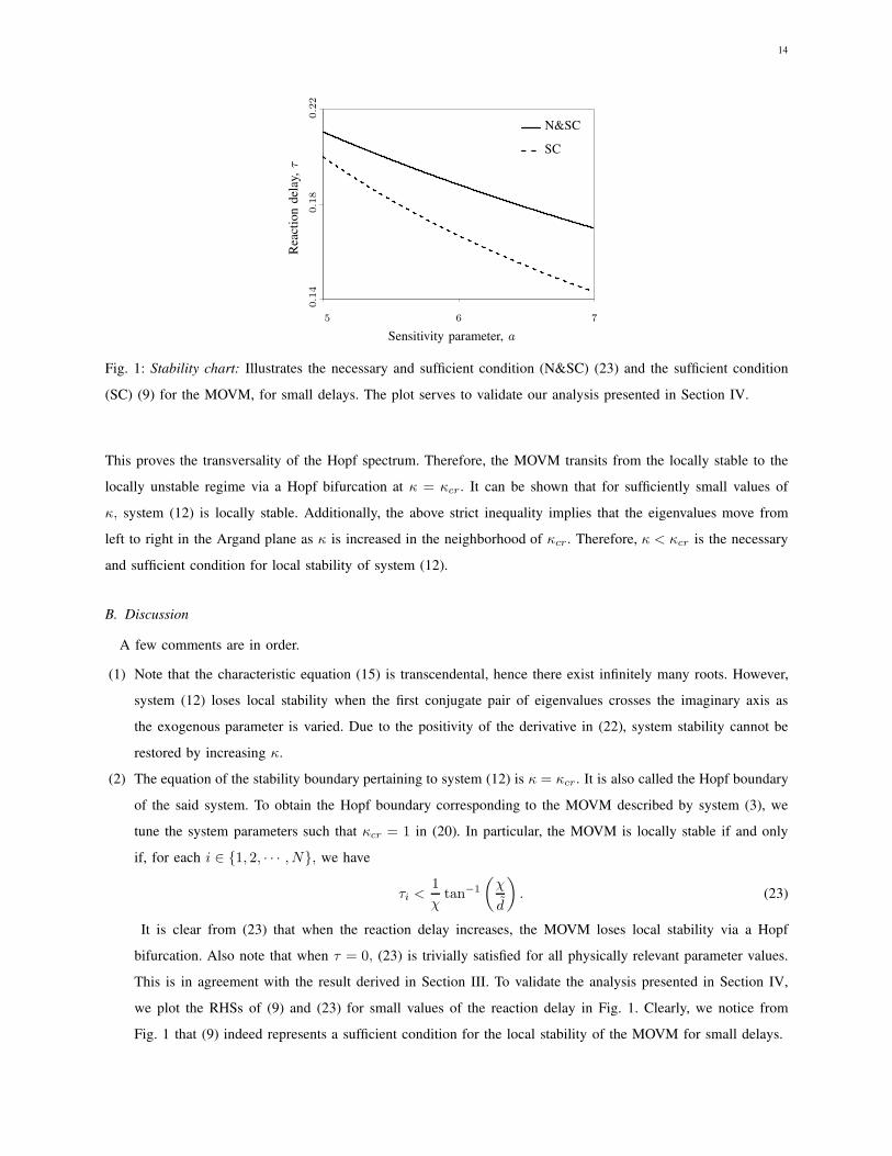
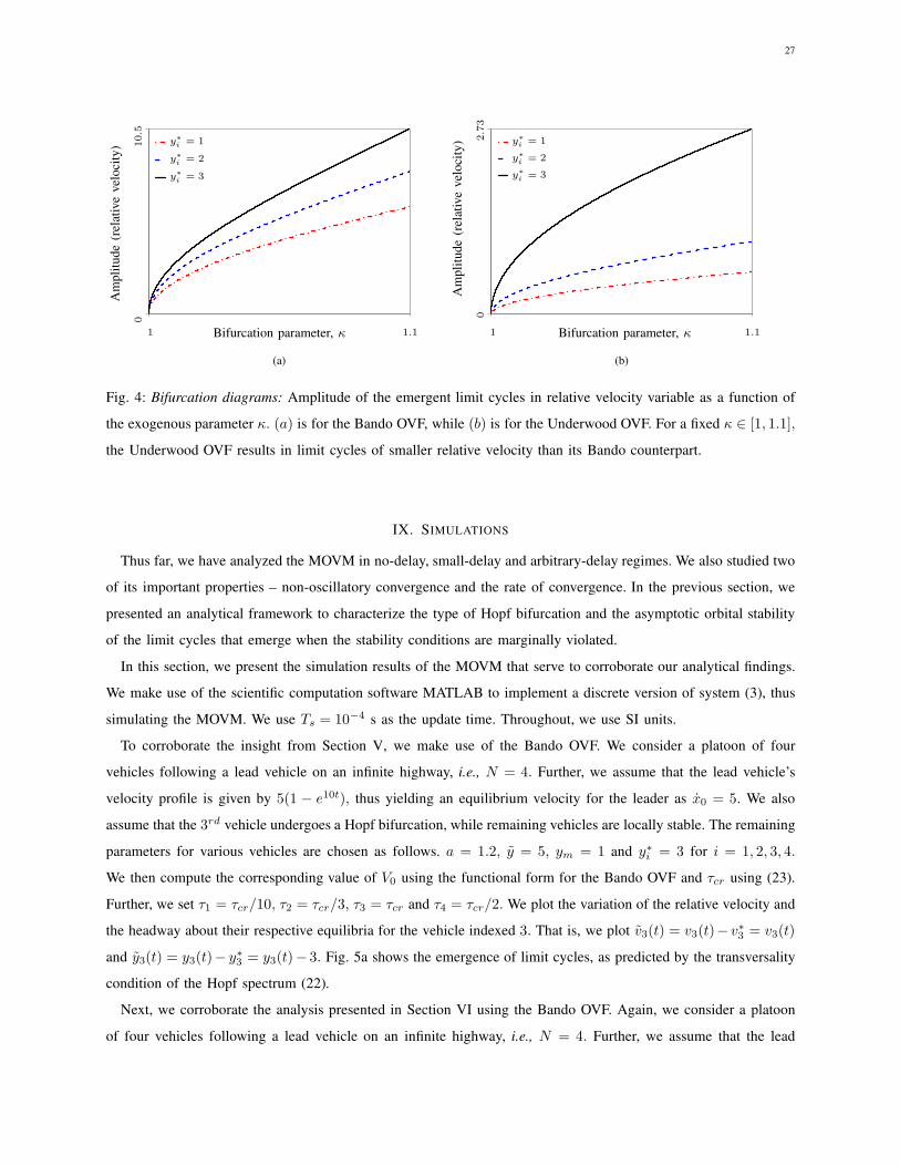
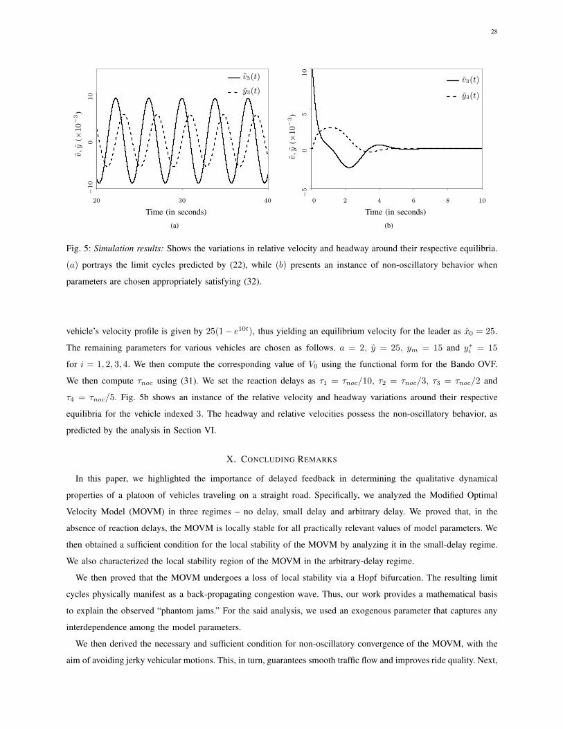
x(t) = f(x(t), x(t − τ1), · · · , x(t− τn)), (10)
12
is modified to
x(t) = κf(x(t), x(t − τ1), · · · , x(t− τn)), (11)
with the introduction of the exogenous parameter. Note that (i) κ has no effect on the equilibrium of system (10),
and (ii) we obtain system (10) by setting κ = 1 in system (11). We first linearize system (11) about its non-trivial
equilibrium and derive its characteristic equation. We then search for a pair of conjugate eigenvalues on the imaginary
axis in the Argand plane. This yields the necessary and sufficient condition for the local stability of system (11).
Setting the exogenous parameter to unity then yields the necessary and sufficient condition for system (10). The
exogenous parameter so introduced helps simplify the requisite algebra and capture any interdependence among the
system parameters.
For the MOVM, introducing κ in (3) yields
v1(t) = x0(t) + κa (x0(t− τ1)− V (y1(t− τ1))− v1(t− τ1)) ,
vk(t) =κa (V (yk−1(t− τk−1))− V (yk(t− τk))− vk(t− τk)) ,
yi(t) =κvi(t), (12)
for i ∈ 1, 2, · · · , N and for k ∈ 2, 3, · · · , N. We linearize this about the equilibrium v∗i = 0, y∗i = V −1(x0),
i = 1, 2, · · · , N, and write it in matrix form to obtain
S(t) =
N∑
k=0
AkS(t− τk), (13)
where the matrices Ak = κAk, for k = 0, 1, · · · , N, where the matrices Ak are as defined in Section II.
The characteristic equation corresponding to system (13) is obtained as [43, Section 5.1]
f(λ) = det
(
λI2N×2N −N∑
k=0
e−λτkAk
)
= 0.
The matrix in consideration is a block matrix of the form
λI2N×2N −N∑
k=0
e−λτkAk =
A B
C D
,
where C = −κIN×N and D = λIN×N . Further, A is a diagonal matrix with the ith diagonal entry being
λ+ κae−λτi , and B is a sparse lower-triangular matrix. Clearly, A and D are invertible, and C commutes with D.
Therefore, the characteristic equation simplifies to the form [44, Theorem 3]
f(λ) = det
A B
C D
= det(
AD − BC)
= 0.
Simplifying the above expression, we obtain the characteristic equation pertaining to (13) as
f(λ) =
N∏
i=1
(λ2 + κaλe−λτi + κ2de−λτi) = 0. (14)
13
For multiple terms in the above product to equal zero, their respective reaction delays must be equal. Such a
possibility is not realistic, hence we ignore it. Therefore, for some i ∈ 1, 2, · · · , N, we have
λ2 + κaλe−λτi + κ2de−λτi = 0. (15)
System (12) will be locally stable if and only if all the roots of (15) lie in the open left-half of the Argand plane [43,
Theorem 5.1.1]. Therefore, we search for a conjugate pair of eigenvalues of (15) that crosses the imaginary axis in
the Argand plane. To that end, we substitute λ = jω in (15), with j =√−1. We then equate the real and imaginary
parts to zero and obtain
κaω sin(ωτi) + κ2d cos(ωτi) =ω2, (16)
κaω cos(ωτi)− κ2d sin(ωτi) = 0. (17)
Squaring and adding (16) and (17) yields ω4 − κ2a2ω2 − κ4d2 = 0. Solving for ω2, we obtain
ω21,2 = κ2
(
a2 ±√a4 + 4d2
2
)
.
Since we are searching for a positive root, we discard the negative root. The positive root of the above expression
is given by
ω = κ
√
a(a+√
a2 + 4d2)
2. (18)
For convenience, we write the above equation as ω = κχ. Notice that, on re-arranging (17), we obtain κd tan(ωτi) =
ω. Substituting for ω in the above equation and simplifying yields
ω0 =1
τitan−1
(χ
d
)
. (19)
Substituting ω0 in (17) and simplifying, we obtain
κcr =1
τiχtan−1
(χ
d
)
. (20)
Thus, (19) and (20) yield the angular frequency of the oscillatory solution and the value of κ at which such a
solution exists respectively.
We now show that the MOVM undergoes a Hopf bifurcation at κ = κcr. To that end, we need to prove the
transversality condition of the Hopf spectrum. That is, we must show that [11, Chapter 11, Theorem 1.1]
Real
(dλ
dκ
)
κ=κcr
6= 0. (21)
To that end, we differentiate (15) with respect to κ and simplify it, to obtain
Real
((dλ
dκ
)−1)
κ=κcr
=κcrω
20τi(κ
2crd cos(ω0τi) + ω2
0)
(κ2crd cos(ω0τi) + ω0)2 + (κ2crd sin(ω0τi))2> 0. (22)
The positivity in (22) follows because cos(ω0τi) = κcrd/(κ2crd
2+ω20) is positive. This expression follows from (17)
using trigonometric manipulations. Also, Real(z) > 0 if and only if Real(1/z) > 0 ∀ z ∈ C. Hence, from (22) we
have
Real
(dλ
dκ
)
κ=κcr
> 0.
14
Sensitivity parameter, a
Rea
ctio
ndel
ay,τ
50.14
0.22
6 70.18
SC
N&SC
Fig. 1: Stability chart: Illustrates the necessary and sufficient condition (N&SC) (23) and the sufficient condition
(SC) (9) for the MOVM, for small delays. The plot serves to validate our analysis presented in Section IV.
This proves the transversality of the Hopf spectrum. Therefore, the MOVM transits from the locally stable to the
locally unstable regime via a Hopf bifurcation at κ = κcr. It can be shown that for sufficiently small values of
κ, system (12) is locally stable. Additionally, the above strict inequality implies that the eigenvalues move from
left to right in the Argand plane as κ is increased in the neighborhood of κcr. Therefore, κ < κcr is the necessary
and sufficient condition for local stability of system (12).
B. Discussion
A few comments are in order.
(1) Note that the characteristic equation (15) is transcendental, hence there exist infinitely many roots. However,
system (12) loses local stability when the first conjugate pair of eigenvalues crosses the imaginary axis as
the exogenous parameter is varied. Due to the positivity of the derivative in (22), system stability cannot be
restored by increasing κ.
(2) The equation of the stability boundary pertaining to system (12) is κ = κcr. It is also called the Hopf boundary
of the said system. To obtain the Hopf boundary corresponding to the MOVM described by system (3), we
tune the system parameters such that κcr = 1 in (20). In particular, the MOVM is locally stable if and only
if, for each i ∈ 1, 2, · · · , N, we have
τi <1
χtan−1
(χ
d
)
. (23)
It is clear from (23) that when the reaction delay increases, the MOVM loses local stability via a Hopf
bifurcation. Also note that when τ = 0, (23) is trivially satisfied for all physically relevant parameter values.
This is in agreement with the result derived in Section III. To validate the analysis presented in Section IV,
we plot the RHSs of (9) and (23) for small values of the reaction delay in Fig. 1. Clearly, we notice from
Fig. 1 that (9) indeed represents a sufficient condition for the local stability of the MOVM for small delays.
15
(3) Loss of local stability via a Hopf bifurcation results in the emergence of limit cycles. Since the dynamical
variables for the MOVM correspond to relative velocities and headways, these non-linear oscillations physically
manifest as back-propagating congestion wave on a highway. Thus, as mentioned in the Introduction, our
analysis provides a mathematical basis to the commonly-observed “phantom jam.”
(4) Note that the non-dimensional parameter κ is not a model parameter; rather, it is an exogenous mathematical
entity introduced to aid the analysis and capture any interdependence among model parameters. It also serves to
simplify the algebra required to obtain the necessary and sufficient condition for local stability of the MOVM.
Further, since substituting κ = 1 yields the MOVM, it is useful in a neighborhood around 1, i.e., near the
stability boundary.
(5) Gain parameters are known to destabilize feedback systems [1, Section 3.7]. Thus, we need to verify that the
bifurcation phenomenon proved in this section is not an artefact of the exogenous parameter. To that end, we
need to verify that the MOVM also undergoes a Hopf bifurcation when one of the model parameters is chosen
as the bifurcation parameter. It was shown in [46] that the transversality condition of the Hopf spectrum holds
true for the characteristic equation of the form (15) (with κ = 1) when τ is used as the bifurcation parameter,
although in a different context.
(6) Note that the non-dimensional parameter κ can also be interpreted as a time-scale change for the case of the
MOVM. This can be seen from (12) by multiplying both sides by 1/κ, and making the change of variable
t = κt. Then, the “relative importance” of the reaction delays to the system time scale would be κτi/t, for each
i. Thus, in this new time scale, an increase in κ can be interpreted as a uniform (multiplicative) increase in all
the reaction delays. Thus, the aforementioned viewpoint may also be useful in interpreting the single-parameter
bifurcation analysis presented in this paper.
VI. NON-OSCILLATORY CONVERGENCE
In the previous three sections, we derived conditions for the MOVM to be locally stable in three different regimes.
In the next two sections, we explore two important properties of the MOVM; namely, non-oscillatory convergence
and the rate of convergence.
In the context of transportation networks, ride quality is of utmost importance. This, in turn, mandates that the
vehicles avoid jerky motion. Since relative velocities and headways constitute dynamical variables for the MOVM,
it boils down to studying the non-oscillatory property of its solutions. In particular, we derive the necessary and
sufficient condition for non-oscillatory convergence of the MOVM. Mathematically, this amounts to ensuring that
the eigenvalues corresponding to system (5) are negative real numbers.
To derive the necessary and sufficient condition for non-oscillatory convergence of the MOVM, we begin with the
characteristic equation corresponding to system (3), obtained by setting κ = 1 in (15). We also drop the subscript
“i” for convenience. Thus, we obtain
f(λ) = λ2 + (aλ+ d)e−λτ = 0. (24)
16
To ensure non-oscillatory convergence of the MOVM, we require the roots of (24) to be real and negative. To
that end, we substitute λ = σ + jω in (24), where j =√−1. This yields
aω sin(ωτ) + (aσ + d) cos(ωτ) = (ω2 − σ2)eστ , and (25)
aω sin(ωτ) + (aσ + d) cos(ωτ) = (−2σω)eστ . (26)
Squaring and adding (25) and (26), we obtain
(aω)2 + (aσ + d)2 = (ω2 + σ2)2e2στ . (27)
To ensure that the roots are real, we require a condition for ω = 0 to be the only solution of (27). Substituting
ω = 0 in (27), we obtain
(aσ + d)2 = σ4e2στ . (28)
Thus, the above condition is necessary for ω = 0 to be a solution of (27). To check whether it is also a sufficient
condition, we first separate the terms containing ω in (27) from those without it. This yields
e2στω4 + (2σ2e2στ − a2)ω2 = (aσ + d)2 − σ4e2στ .
Assuming (aσ + d)2 = σ4e2στ , we solve the above quadratic in ω2 to obtain
ω2 = 0 or ω2 =a2 − 2σ2e2στ
e2στ.
Thus, for ω = 0 to be the unique solution of (27), we require a2 = 2σ2e2στ in addition to the condition mentioned
in (28). That is, (24) has real eigenvalues if and only if
(aσ + d)2 = σ4e2στ , and a2 = 2σ2e2στ . (29)
Solving the above two equations for the eigenvalue, we obtain
σ = dm±, with m± = −2±√2. (30)
Notice from the foregoing analysis that the eigenvalues are guaranteed to be negative if they are real. Substituting (30)
in (24) and re-arranging, we obtain the boundary for the region of non-oscillatory convergence as
e−dτm± =−m2
±d
a(m+ 1).
Notice that the Left Hand Side (LHS) in the above equation is a non-negative quantity. The RHS is non-negative
for m− but not for m+. Hence, we set m = m− in the above equation, and re-arrange to obtain
τnoc =1
mdln
(−a(m+ 1)
m2d
)
, (31)
where τnoc represents the boundary for the region of non-oscillatory convergence in the τ -domain. Therefore,
τ < τnoc represents the necessary and sufficient condition for non-oscillatory convergence of the MOVM. We note
that the following inequalities must be satisfied: 0 < τnoc < τcr, where τcr is the RHS of (23).
In summary, the necessary and sufficient condition for non-oscillatory convergence of the MOVM is
τi <1
mdln
(−a(m+ 1)
m2d
)
, (32)
17
Rea
ctio
ndel
ay,τ
Sensitivity coefficient, a
0.4
0.3
0.2
0.1
1 2 3 4 5
τnoc
τcr
Fig. 2: Illustration of the region of non-oscillatory convergence for the MOVM. Here, τcr and τnoc represent the
boundaries of the locally stable region and the region of non-oscillatory convergence of the MOVM respectively.
Notice the stringent requirements on the reaction delay for the solutions of the MOVM to be non oscillatory, for a
given sensitivity coefficient.
for each i ∈ 1, 2, · · · , N, when the RHS is positive and less than τcr.
We now illustrate the boundary for the region of non-oscillatory convergence of the MOVM described by (31). In
order to better-understand the stringent constraints on system parameters to achieve non-oscillatory convergence, we
also plot the necessary and sufficient condition for local stability (23) of the MOVM. To that end, we make use of
the Bando OVF. We let the equilibrium velocity of the lead vehicle to be x0 = 5 m/s, and the model parameters as
y∗ = 2 m, y = 5 m and ym = 1 m. We then compute the corresponding V0 and d. We vary the sensitivity coefficient
a from 1 and 5, and compute the requisite boundaries using the scientific computation software MATLAB.
Fig. 2 portrays regions of local stability and non-oscillatory convergence for the MOVM in the (a, τ)-space. For a
fixed a, the reaction delay must not exceed τcr (respectively, τnoc) for the MOVM to be locally stable (respectively,
possess non-oscillatory solutions). Clearly, the values of τ need to be much smaller for the solutions of the MOVM
to be non oscillatory as opposed to the stability of the MOVM, for a fixed value of a. In fact, as the sensitivity
parameter a increases, the corresponding value of reaction delays required to ensure non-oscillatory convergence
decreases rapidly.
We end this section with two remarks. (i) To the best of our knowledge, the analysis presented in this section
is the first to address non-oscillatory convergence of systems with characteristic equations of the form (24) using
spectral-domain techniques, and (ii) we can obtain ω = 0 as the only solution to (27) by a geometrical method as
follows. Re-arranging (27) yields
(ω2 + σ2)2 = (a2e−2στ )ω2 + (aσ + d)2e−2στ .
Notice that the LHS and the RHS of the above equation represent a parabola and a line in ω2 respectively. Since
a parabola is strictly convex, the tangent to a parabola at any point will intersect it only at that point. It can be
18
shown that the RHS of the above equation will be the tangent to the LHS at ω2 = 0 if and only if the conditions
in (29) hold. Details of this approach can be found in the technical report [49].
VII. RATE OF CONVERGENCE
In this section, we characterize the time required to attain the uniform traffic flow, once the traffic flow is
perturbed (by events such as the departure of a vehicle from the platoon). Mathematically, it is related to the rate of
convergence of solutions of the MOVM to the desired equilibrium. To that end, we follow [47] and first characterize
the rate of convergence of the MOVM. Then, using the notion of settling time, we derive an expression for the
time a platoon takes to attain the desired equilibrium following a perturbation.
We begin by recalling the characteristic equation pertaining to system (5) from Section V-A. Dropping the
subscript “i” for ease of exposition, and setting κ = 1 in (15), we obtain
λ2 + aλe−λτ + de−λτ = 0.
Using the change of variables z = λτ, the above equation results in
z2ez + a∗z + d∗ = 0, (33)
where a∗ = aτ and d∗ = dτ2. Notice that (33) has the same form as [47, Equation (22)]. Hence, following [47],
we substitute z = ψ − σ, where σ is non-negative and real, in (33) to obtain
(ψ2 − 2σψ + σ2)eψ + a∗eσψ + (d∗ − a∗σ)eσ = 0.
The characteristic equation corresponding to the above system is obtained by substituting ψ = τλ as
λ2 +
(
−2σ
τ
)
λ+ (aeσ)λe−λτ +(
d− aσ
τ
)
eσe−λτ +
(σ2
τ2
)
= 0. (34)
The rate of convergence is the largest σ ≥ 0 such that the root of (34) with the largest real part is negative [47].
As pointed out in [47], finding such a σ analytically is intractable. Hence, we illustrate the variation of the rate
of convergence numerically with respect to both the sensitivity parameter a and the reaction delay τ , using the
scientific computation software MATLAB.
We consider the Bando OVF, and set the following parameters: ym = 1 m, y = 5 m, y∗ = 2 m and x0 = 5 m/s.
We then compute the corresponding values of V0 and d. Next, we vary the sensitivity coefficient a in the range
[1, 5], and for each of its values, we compute the critical value of the reaction delay τcr using (23). We then vary the
reaction delay τ in the range [0, τcr], for each a. For every pair (a, τ) in this range, σ is increased from 0, till the
root of (34) with the largest real part crosses the imaginary axis in the Argand plane. Since the resulting plot would
be three dimensional, we present the corresponding contour plots in Fig. 3. For clarity in presentation, the contour
plots are segregated as follows: Fig. 3a is for low to medium values of the rate of convergence, whereas Fig. 3b is
for high values. It can be seen from Fig. 3a that small changes in a or τ causes the rate of convergence to change
from 0.3 to 0.9. However, it would require relatively larger changes in a or τ for the rate of convergence to change
from 0.1 to 0.3. That is, the gradient of the rate of convergence increases rather rapidly with an increase in the rate
of convergence. Also, for low values of the rate of convergence, non-oscillatory convergence can be guaranteed. In
19
0.1
0.3
0.9
Rea
ctio
ndel
ay,τ
Sensitivity coefficient, a
τcrτnoc
00.1
0.2
0.3
0.4
1 2 3 4 5
(a)
1.1 1.2
Rea
ctio
ndel
ay,τ
Sensitivity coefficient, a
τcr
τnoc
0.1
0.2
0.3
0.4
2 3 4
(b)
Fig. 3: Contour plots: Contour lines of the rate of convergence overlaying the boundaries of the locally stable
region and the region of non-oscillatory convergence of the MOVM. While (a) is for low to medium values of
rate of convergence, (b) is for high values. From (a), observe: (i) the rapid change in the gradient of the rate of
convergence, and (ii) for lower values of the rate of convergence, non-oscillatory convergence is also guaranteed. In
contrast, (b) shows that very high rates of convergence cannot be achieved if the solutions are to be non oscillatory.
contrast, Fig. 3b brings forth the trade-off between the rate of convergence and non-oscillatory convergence; very
high rates of convergence cannot be achieved if the solutions are to be non oscillatory.
The rate of convergence determines the time taken by a platoon to reach an equilibrium (denoted by T eMOVM ).
To characterize T eMOVM , we first define the time taken by the ith pair of vehicles in the platoon following the
standard control-theoretic notion of “settling time.” That is, by tei (ǫ), we denote the minimum time taken by the
time-domain trajectory of the MOVM to enter and subsequently remain within the ǫ-band around the equilibrium.
For simplicity, we drop the explicit dependence on ǫ. Then,
T eMOVM =
N∑
i=1
tei . (35)
It is clear that (35) is an upper bound on the time taken by the platoon to equilibrate. However, the equality holds
since the ith pair cannot equilibrate till the (i− 1)th pair has reached its equilibrium.
VIII. HOPF BIFURCATION ANALYSIS
In the previous sections, we have characterized the stable region for the MOVM, and studied two of its most
important properties; namely, non-oscillatory convergence and the rate of convergence. We have also proved that
system (3) loses stability via a Hopf bifurcation, thus resulting in limit cycles. In this section, we provide an
analytical framework to characterize the type of the bifurcation and the asymptotic orbital stability of the emergent
limit cycles. We closely follow the style of analysis presented in [39], which uses Poincare normal forms and the
center manifold theory.
20
We begin by denoting the RHS of (12) as fi. That is, for i ∈ 1, 2, · · · , N,
fi , aκ (V (yi−1(t− τi−1))− V (yi(t− τi))− vk(t− τi)) . (36)
Define µ = κ− κcr. Notice that the system undergoes a Hopf bifurcation at µ = 0, where κ = κcr. Henceforth,
we shall consider µ as the bifurcation parameter. Also, it is clear that when µ > 0, the exogenous parameter κ
changes from κcr to κcr + µ, thus pushing the system into an unstable regime.
We now provide a step-by-step overview of the detailed local bifurcation analysis, before delving into its technical
details.
Step 1: We begin by applying Taylor’s series expansion to the RHS of (36). Next, we separate the linear terms
from their non-linear counterparts. This allows us to cast the resulting equation into the standard form of an Operator
Differential Equation (OpDE).
Step 2: When µ = 0, the system has exactly one pair of purely imaginary eigenvalues with non-zero angular
velocity, as seen from (22). We call the linear space spanned by the corresponding eigenvectors as the critical
eigenspace. For the purpose of our analysis, we also require a locally invariant manifold that is a tangent to the
critical eigenspace at the system’s equilibrium. The center manifold theorem [39] guarantees the existence of such
a manifold.
Step 3: Next, we project the system onto its critical eigenspace and its complement when µ = 0. Thus, we may
write the dynamics of the original system on the center manifold as an ODE in a single complex variable.
Step 4: Finally, using Poincare normal forms, we evaluate the Lyapunov coefficient and the Floquet exponent.
These, in turn, help characterize the type of the Hopf bifurcation and the asymptotic orbital stability of the emergent
limit cycles.
We begin the analysis by expanding (12) about the equilibrium v∗i = 0, y∗i = V −1(x0), i = 1, 2, · · · , N, using
Taylor’s series, to obtain
vi(t) =(−κa)vi,t(−τi) +(
−κaV ′
(y∗i ))
yi,t(−τi) +(
−κaV ′′
(y∗i ))
y2i,t(−τi)
+(
−κaV ′′′
(y∗i ))
y3i,t(−τi) + ζ(1)i y(i−1),t(−τi−1) + ζ
(2)i y2(i−1),t(−τi−1)
+ ζ(3)i y3(i−1),t(−τi−1) + higher order terms,
yi(t) =κxi(t) (37)
where we use the shorthand vi,t(−τi) and yi,t(−τi) to represent vi(t − τi) and yi(t − τi) respectively. Also, V′
,
V′′
and V′′′
denote the first, second and third derivatives of the OVF with respect to the state variable respectively.
Additionally, the coefficients ζ(1)i , ζ
(2)i and ζ
(3)i represent −κaV ′
(y∗i ), −κaV′′
(y∗i ) and −κaV ′′′
(y∗i ) respectively
for i > 1, and are zero for i = 1.
In the following, we use Ck (A;B) to denote the linear space of all functions from A to B which are k times
differentiable, with each derivative being continuous. Also, we use C to denote C0, for convenience.
With the concatenated state S(t), note that (12) is of the form:
dS(t)
dt= LµSt(θ) + F(St(θ), µ), (38)
21
where t > 0, µ ∈ R, and where for τ = maxiτi > 0,
St(θ) = S(t+ θ), S : [−τ, 0] −→ R2N , θ ∈ [−τ, 0].
Here, Lµ : C([−τ, 0];R2N
)−→ R2N is a one-parameter family of continuous, bounded linear functionals, whereas
the operator F : C([−τ, 0];R2N
)−→ R2N is an aggregation of the non-linear terms. Further, we assume that
F(St, µ) is analytic, and that F and Lµ depend analytically on the bifurcation parameter µ, for small |µ|. The
objective now is to cast (38) in the standard form of an OpDE:
dSt
dt= A(µ)St +RSt, (39)
since the dependence here is on St alone rather than both St and S(t). To that end, we begin by transforming the
linear problem dS(t)/dt = LµSt(θ). We note that, by the Riesz representation theorem [48, Theorem 6.19], there
exists a 2N × 2N matrix-valued measure η(·, µ) : B(C([−τ, 0];R2N
))−→ R2N×2N , wherein each component of
η(·) has bounded variation, and for all φ ∈ C([−τ, 0];R2N
), we have
Lµφ =
0∫
−τ
dη(θ, µ)φ(θ). (40)
In particular,
LµSt =
0∫
−τ
dη(θ, µ)S(t+ θ).
Motivated by the linearized system (13), we define
dη =
A B
C D
dθ,
where
(A)ij =
−κdδ(θ + τi), i = j,
κdδ(θ + τj), j = i− 1, i > 1,
0, otherwise,
(B)ij =
−κaδ(θ + τi), i = j,
0, otherwise,
C = κIN×N and D = 0N×N .
For φ ∈ C1([−τ, 0];C2N
), we define
A(µ)φ(θ) =
dφ(θ)dθ
, θ ∈ [−τ, 0),0∫
−τ
dη(s, µ)φ(s) ≡ Lµ, θ = 0,(41)
and
Rφ(θ) =
0, θ ∈ [−τ, 0),
F(φ, µ), θ = 0.
22
With the above definitions, we observe that dSt/dθ ≡ dSt/dt. Hence, we have successfully cast (38) in the form
of (39). To obtain the required coefficients, it is sufficient to evaluate various expressions for µ = 0, which we
use henceforth. We start by finding the eigenvector of the operator A(0) with eigenvalue λ(0) = jω0. That is, we
want an 2N × 1 vector (to be denoted by q(θ)) with the property that A(0)q(θ) = jω0q(θ). We assume the form:
q(θ) = [1 φ1 φ2 · · · φ2N−1]T ejω0θ, and solve the eigenvalue equations. We also assume the following:
(i)
− jω0ejω0τ1 + κd
κ2a=
−1 + ejω0τ
ω20
,
(ii) For each i ∈ 1, 2, · · ·N − 1, the following matrix is invertible:
κde−jω0τi+1 + jω0 κae−jω0τi+1
κβ −jω0
,
where β = j(−1 + je−jω0τ )/ω0. Then, for i ∈ 1, 2, · · ·N − 1,
φN =κβ
jω0, φi = − jκω0de
−jω0τi
∆Mi
, and φN+i = −βκ2de−jω0τi
∆Mi
,
where ∆Mi = ω20 − κdω0 sin(ω0τi+1)− κ2βa cos(ω0τi+1) + j
(κ2βa sin(ω0τi+1)− κdω0 cos(ω0τi+1)
).
We define the adjoint operator as follows:
A∗(0)φ(θ) =
− dφ(θ)dθ
, θ ∈ (0, τ ],0∫
−τ
dηT (s, 0)φ(−s), θ = 0,
where dηT is the transpose of dη.
We note that the domains of A and A∗ are C1([−τ, 0];C2N
)and C1
([0, τ ];C2N
)respectively. Therefore, if jω0
is an eigenvalue of A, then −jω0 is an eigenvalue of A∗. Hence, to find the eigenvector of A∗(0) corresponding
to −jω0 (to be denoted by p(θ)), we assume the form: p(θ) = B[ψ2N−1 ψ2N−2 ψ2N−3 · · · 1]T ejω0θ, and solve
A∗(0)p(θ) = −jω0p(θ). We also assume the following:
(i)
κd− jω0ejω0τN
κ2a=
−1 + ejω0τ
ω20
,
(ii) For each i ∈ 1, 2, · · ·N − 1, the following matrix is invertible:
jω0 −κae−jω0τi
κβ κde−jω0τi − jω0
.
Then, for i ∈ 1, 2, · · ·N − 1, we obtain
ψN =jω0e
jω0τN
κa, ψN+i =
jω0κdψN+i−1e−jω0τN−i
∆Mi
, and ψi =κ2adψN+i−1e
−jω0τN−i
∆Mi
,
where ∆Mi = ω20 + κdω0 sin(ω0τN−i) + κ2βa cos(ω0τN−i) + j
(κdω0 cos(ω0τN−i)− κ2βa sin(ω0τN−i)
).
The normalization condition for Hopf bifurcation requires that 〈p, q〉 = 1, thus yielding an expression for B.
23
For any q ∈ C([−τ, 0];C2N
)and p ∈ C
([0, τ ];C2N
), the inner product is defined as
〈p, q〉 , p · q −0∫
θ=−τ
θ∫
ζ=0
pT (ζ − θ)dηq(ζ) dζ, (42)
where the overbar represents the complex conjugate and the “ · ” represents the regular dot product. The value of
B such that the inner product between the eigenvectors of A and A∗ is unity can be shown to be
B =1
ζ1 + ζ2 + ζ3 + ζ4,
where
ζ1 =
(2ejω0τ − ej2ω0τ − 1
2
)N−1∑
i=0
κψN−i−1φi, ζ2 =
N−1∑
i=0
(ejω0τi+1 − ej2ω0τi+1
jω0
)
κψ2N−1−i(aφi + dφN+i),
ζ3 =
N−2∑
i=0
(ej2ω0τi+1 − ejω0τi+1
jω0
)
κdφiψ2N−2−i, and, ζ4 =
2N−1∑
i=0
ψ2N−1−iφi.
For St, a solution of (39) at µ = 0, we define
z(t) = 〈p(θ), St〉, and w(t, θ) = St(θ)− 2Real(z(t)q(θ)).
Then, on the center manifold C0, we have w(t, θ) = w(z(t), z(t), θ), where
w(z(t), z(t), θ) = w20(θ)z2
2+ w02(θ)
z2
2+ w11(θ)zz + · · · . (43)
Effectively, z and z are the local coordinates for C0 in C in the directions of p and p respectively. We note that
w is real if St is real, and we deal only with real solutions. The existence of the center manifold C0 enables the
reduction of (39) to an ODE in a single complex variable on C0. At µ = 0, the said ODE can be described as
z(t) = 〈p,ASt +RSt〉 ,
= jω0z(t) + p(0).F (w(z, z, θ) + 2Real(z(t)q(θ))) ,
= jω0z(t) + p(0).F0(z, z). (44)
This is written in abbreviated form as
z(t) = jω0z(t) + g(z, z). (45)
The objective now is to expand g in powers of z and z. However, this requires wij(θ)’s from (43). Once these are
evaluated, the ODE (44) for z would be explicit (as given by (45)), where g can be expanded in terms of z and z
as
g(z, z) = p(0).F0(z, z) = g20z2
2+ g02
z2
2+ g11zz + g21
z2z
2+ · · · . (46)
Next, we write w = St − zq − ˙zq. Using (39) and (45), we then obtain the following ODE:
w =
Aw − 2Real(p(0).F0q(θ)), θ ∈ [−τ, 0),
Aw − 2Real(p(0).F0q(0)) + F0, θ = 0.
24
This can be re-written using (43) as
w = Aw +H(z, z, θ), (47)
where H can be expanded as
H(z, z, θ) = H20(θ)z2
2+H02(θ)
z2
2+H11(θ)zz +H21(θ)
z2z
2+ · · · . (48)
Near the origin, on the manifold C0, we have w = wz z + wz ˙z. Using (43) and (45) to replace wz z (and their
conjugates, by their power series expansion) and equating with (47), we obtain the following operator equations:
(2jω0 −A)w20(θ) =H20(θ), (49)
−Aw11 =H11(θ), (50)
−(2jω0 +A)w02(θ) =H02(θ). (51)
We start by observing that
St(θ) = w20(θ)z2
2+ w02(θ)
z2
2+ w11(θ)zz + zq(θ) + zq(θ) + · · · .
From the Hopf bifurcation analysis [39], we know that the coefficients of z2, z2, z2z, and zz terms are used to
approximate the system dynamics. Hence, we only retain these terms in the expansions.
To obtain the effect of non-linearities, we substitute the aforementioned terms appropriately in the non-linear
terms of (37) and separate the terms as required. Therefore, for each i ∈ 1, 2, · · · , 2N, we have the non-linearity
term to be
Fi = F20iz2
2+ F02i
z2
2+ F11izz + F21i
z2z
2, (52)
where, for i ∈ 1, 2, · · · , N, the coefficients are given by
F20i = Ω(1)i w20i(−τi) + ζ
(1)i−1w20(i−1)(−τi−1),
F02i = Ω(1)i w02i(−τi) + ζ
(1)i−1w02(i−1)(−τi−1),
F11i = Ω(1)i w11i(−τi) + ζ
(1)i−1w11(i−1)(−τi−1),
F21i = 2Ω(2)i
(w20i(−τi)ejω0τi + 2w11i(−τi)e−jω0τi
)
+ 2ζ(2)i−1
(w20(i−1)(−τi−1)e
jω0τi−1 + 2w11(i−1)(−τi−1)e−jω0τi−1
),
and for i ∈ N + 1, N + 2, · · · , 2N, each of these coefficients is zero. This is so, since last N states correspond
to the headways who evolution equations are linear. Here, Ω(1)i = −κaV ′
(y∗i ), Ω(2)i = −κaV ′′
(y∗i ), and Ω(3)i =
−κaV ′′′
(y∗i ).
Next, we compute g in (45) as
g(z, z) = p(0).F0 = B
2N∑
l=1
ψ2N−lFl, (53)
25
where F0 = [F1 F2 · · · F2N ]T . Substituting (52) in (53), and comparing with (46), we obtain
gx = B2N∑
l=1
ψ2N−lFxl, (54)
where x ∈ 20, 02, 11, 21. Using (54), the corresponding coefficients can be computed. However, computing g21
requires w20(θ) and w11(θ). Hence, we perform the requisite computation next. For θ ∈ [−τ, 0), H can be simplified
as
H(z, z, θ) = −Real (p(0).F0q(θ)) ,
= −(
g20z2
2+ g02
z2
2+ g11zz + · · ·
)
q(θ)
−(
g20z2
2+ g02
z2
2+ g11zz + · · ·
)
q(θ),
which, when compared with (48), yields
H20(θ) = −g20q(θ)− g20q(θ), (55)
H11(θ) = −g11q(θ)− g11q(θ). (56)
From (41), (49) and (50), we obtain the following ODEs:
w20(θ) = 2jω0w20(θ) + g20q(θ) + g02q(θ), (57)
w11(θ) = g11q(θ) + g11q(θ). (58)
Solving (57) and (58), we obtain
w20(θ) = − g20jω0
q(0)ejω0θ − g023jω0
q(0)e−jω0θ + e e2jωθ, (59)
w11(θ) =g11jω0
q(0)ejω0θ − g11jω0
q(0)e−jω0θ + f, (60)
for some vectors e and f, to be determined.
To that end, we begin by defining the following vector: F20 , [F201 F202 · · · F20(2N)]T . Equating (49) and (55),
and simplifying, yields the operator equation: 2jω0e − A(e e2jω0θ
)= F20. To solve this, we assume that the
following matrices to be invertible for each i ∈ 1, 2, · · · , N,
2jωo + κ(a+ d)e−jω0τi κ(a+ d)e−jω0τi
−κτ 2jωo
.
Under this condition, we obtain for i ∈ 1, 2, · · · , N,
ei =2jω0F20i
∆M∗i
, and, eN+i =κτF20i
∆M∗i
, (61)
where ∆M∗i = −4ω2
0 + 2ω0κ(a + d) sin(ω0τi) + τκ2(a + d) cos(ω0τi) + j(2ω0κ(a + d) cos(ω0τi) − τκ2(a +
d) sin(ω0τi)).
Next, equating (50) and (56), and simplifying, we obtain the operator equation Af = −F11, with F11 ,
[F111 F112 · · · F11(2N)]T . On solving this equation, we obtain for i ∈ 1, 2, · · · , N,
fi = 0, and, fN+i =F11i
κτi(a+ d). (62)
26
Substituting for e and f from (61) and (62) in (59) and (60) respectively, we obtain w20(θ) and w11(θ). This, in
turn, facilitates the computation of g21. We can then compute
c1(0) =j
2ω0
(
g20g11 − 2|g11|2 −1
3|g02|2
)
+g212,
α′
(0) = Real
(dλ
dκ
)
κ=κcr
, µ2 = −Real(c1(0))
α′(0), and β2 = 2Real(c1(0)).
Here, c1(0) is known as the Lyapunov coefficient and β2 is the Floquet exponent. It is known from [39] that
these quantities are useful since
(i) If µ2 > 0, then the bifurcation is supercritical, whereas if µ2 < 0, then the bifurcation is subcritical.
(ii) If β2 > 0, then the limit cycle is asymptotically orbitally unstable, whereas if β2 < 0, then the limit cycle is
asymptotically orbitally stable.
Some of the details pertaining to the derivation can be found in the technical report [49]. We now present
numerically-constructed bifurcation diagrams to gain some insight into the effect of various parameters on the
amplitude of the limit cycle.
Bifurcation diagrams
To obtain bifurcation diagrams, we make use of DDE-BIFTOOL [50], [51]. We first input system (12) and their
first-order derivatives with respect to the state and delayed state variables to DDE-BIFTOOL. We then set κ = 1
and initialize the model parameters appropriately. We also fix a range of variation for the bifurcation parameter.
DDE-BIFTOOL varies the bifurcation parameter accordingly and finds its critical value. We then increase the value
of κ and record the amplitude of the resulting limit cycle, thus obtaining the bifurcation diagram. We use the SI
units throughout; time will be expressed in “seconds,” distance in “meters,” velocity in “meters per second” and the
sensitivity coefficient in “inverse second.” For our comparison, we consider two optimal velocity functions; namely,
the Bando OVF and the Underwood OVF.
For the Bando OVF, we initialize the parameters as follows: N = 4, a = 1.2, τ1 = 0.2, τ2 = 0.2, τ3 = 0.3911
and τ4 = 0.2. We fix ym = 2 and y = 5, and compute V0 for each of y∗i = 1, 2 and 3. The vehicle indexed 3 is
considered to undergo a Hopf bifurcation. For the case of the Underwood OVF, we set the following values for
the parameters. N = 3, a = 1.2, τ1 = 0.1, τ2 = 0.11885 and τ3 = 0.1. We fix ym = 2, and compute V0 for
each of y∗i = 1, 2 and 3. The vehicle indexed 2 is then considered to undergo a Hopf bifurcation. We choose the
equilibrium velocity of the lead vehicle, x0 = 5.
The bifurcation diagrams are shown in Fig. 4. As seen from the figure, the amplitude of the relative velocity
increases with an increase in κ. However, for a fixed value of the exogenous parameter, the Underwood OVF
yields limit cycles with smaller relative velocity than its Bando counterpart, which is desirable. Also, notice that
the amplitude of the emergent limit cycles increases with an increase in the equilibrium headway. This is intuitive
because larger equilibrium headways offer more space for the resulting limit cycles to oscillate in.
27
Am
pli
tude
(rel
ativ
evel
oci
ty)
Bifurcation parameter, κ
010.5
1.11
y∗i = 1
y∗i = 2
y∗i = 3
(a)
Am
pli
tude
(rel
ativ
evel
oci
ty)
02.73
1 1.1Bifurcation parameter, κ
y∗i = 1
y∗i = 2
y∗i = 3
(b)
Fig. 4: Bifurcation diagrams: Amplitude of the emergent limit cycles in relative velocity variable as a function of
the exogenous parameter κ. (a) is for the Bando OVF, while (b) is for the Underwood OVF. For a fixed κ ∈ [1, 1.1],
the Underwood OVF results in limit cycles of smaller relative velocity than its Bando counterpart.
IX. SIMULATIONS
Thus far, we have analyzed the MOVM in no-delay, small-delay and arbitrary-delay regimes. We also studied two
of its important properties – non-oscillatory convergence and the rate of convergence. In the previous section, we
presented an analytical framework to characterize the type of Hopf bifurcation and the asymptotic orbital stability
of the limit cycles that emerge when the stability conditions are marginally violated.
In this section, we present the simulation results of the MOVM that serve to corroborate our analytical findings.
We make use of the scientific computation software MATLAB to implement a discrete version of system (3), thus
simulating the MOVM. We use Ts = 10−4 s as the update time. Throughout, we use SI units.
To corroborate the insight from Section V, we make use of the Bando OVF. We consider a platoon of four
vehicles following a lead vehicle on an infinite highway, i.e., N = 4. Further, we assume that the lead vehicle’s
velocity profile is given by 5(1 − e10t), thus yielding an equilibrium velocity for the leader as x0 = 5. We also
assume that the 3rd vehicle undergoes a Hopf bifurcation, while remaining vehicles are locally stable. The remaining
parameters for various vehicles are chosen as follows. a = 1.2, y = 5, ym = 1 and y∗i = 3 for i = 1, 2, 3, 4.
We then compute the corresponding value of V0 using the functional form for the Bando OVF and τcr using (23).
Further, we set τ1 = τcr/10, τ2 = τcr/3, τ3 = τcr and τ4 = τcr/2. We plot the variation of the relative velocity and
the headway about their respective equilibria for the vehicle indexed 3. That is, we plot v3(t) = v3(t)− v∗3 = v3(t)
and y3(t) = y3(t)− y∗3 = y3(t)− 3. Fig. 5a shows the emergence of limit cycles, as predicted by the transversality
condition of the Hopf spectrum (22).
Next, we corroborate the analysis presented in Section VI using the Bando OVF. Again, we consider a platoon
of four vehicles following a lead vehicle on an infinite highway, i.e., N = 4. Further, we assume that the lead
28
v,y
(×10−3)
Time (in seconds)
−10
010
20 30 40
v3(t)
y3(t)
(a)
v,y
(×10−3)
Time (in seconds)
0
05
10
−5
102 64 8
v3(t)
y3(t)
(b)
Fig. 5: Simulation results: Shows the variations in relative velocity and headway around their respective equilibria.
(a) portrays the limit cycles predicted by (22), while (b) presents an instance of non-oscillatory behavior when
parameters are chosen appropriately satisfying (32).
vehicle’s velocity profile is given by 25(1− e10t), thus yielding an equilibrium velocity for the leader as x0 = 25.
The remaining parameters for various vehicles are chosen as follows. a = 2, y = 25, ym = 15 and y∗i = 15
for i = 1, 2, 3, 4. We then compute the corresponding value of V0 using the functional form for the Bando OVF.
We then compute τnoc using (31). We set the reaction delays as τ1 = τnoc/10, τ2 = τnoc/3, τ3 = τnoc/2 and
τ4 = τnoc/5. Fig. 5b shows an instance of the relative velocity and headway variations around their respective
equilibria for the vehicle indexed 3. The headway and relative velocities possess the non-oscillatory behavior, as
predicted by the analysis in Section VI.
X. CONCLUDING REMARKS
In this paper, we highlighted the importance of delayed feedback in determining the qualitative dynamical
properties of a platoon of vehicles traveling on a straight road. Specifically, we analyzed the Modified Optimal
Velocity Model (MOVM) in three regimes – no delay, small delay and arbitrary delay. We proved that, in the
absence of reaction delays, the MOVM is locally stable for all practically relevant values of model parameters. We
then obtained a sufficient condition for the local stability of the MOVM by analyzing it in the small-delay regime.
We also characterized the local stability region of the MOVM in the arbitrary-delay regime.
We then proved that the MOVM undergoes a loss of local stability via a Hopf bifurcation. The resulting limit
cycles physically manifest as a back-propagating congestion wave. Thus, our work provides a mathematical basis
to explain the observed “phantom jams.” For the said analysis, we used an exogenous parameter that captures any
interdependence among the model parameters.
We then derived the necessary and sufficient condition for non-oscillatory convergence of the MOVM, with the
aim of avoiding jerky vehicular motions. This, in turn, guarantees smooth traffic flow and improves ride quality. Next,
29
we characterized the rate of convergence of the MOVM, which affects the time taken by a platoon to equilibrate.
We also brought forth the trade-off between the rate of convergence and non-oscillatory convergence of the MOVM.
Finally, we provided an analytical framework to characterize the type of Hopf bifurcation and the asymptotic
orbital stability of the limit cycles which emerge when the stability conditions are violated. Therein, we made
use of Poincare normal forms and the center manifold theory. We corroborated our analyses using stability charts,
bifurcation diagrams, numerical computations and simulations conducted using MATLAB.
Avenues for further research
There are numerous avenues that merit further investigation. In this work, we have derived the conditions for
pairwise stability of vehicles in a platoon, whose dynamics are captured by the MOVM. However, the string stability
of such a platoon remains to be studied.
From a practical standpoint, the parameters of the MOVM may vary, for varied reasons. Hence, it becomes im-
perative that the longitudinal control algorithm be robust to such parameter variations, and to unmodeled dynamics.
ACKNOWLEDGEMENTS
This work is undertaken as a part of an Information Technology Research Academy (ITRA), Media Lab Asia,
project titled “De-congesting India’s transportation networks.” The authors are also thankful to Debayani Ghosh,
Rakshith Jagannath and Sreelakshmi Manjunath for many helpful discussions.
REFERENCES
[1] R. Rajamani, “Vehicle Dynamics and Control,” Springer, Second Edition, 2012.
[2] A. Vahidi and A. Eskandarian, “Research advances in intelligent collision avoidance and adaptive cruise control,” IEEE Transactions on
Intelligent Transportation Systems, vol. 4, pp. 143-153 , 2003.
[3] S. Greengard, “Smart transportation networks drive gains,” Communications of the ACM, vol. 58, pp. 25-27, 2015.
[4] V.A.C. van den Berg and E.T. Verhoef, “Autonomous cars and dynamic bottleneck congestions: The effects on capacity, value of time and
preference heterogeneity,” Transportation Research Part B, vol. 94, pp. 43-60 , 2016.
[5] D.C. Gazis, R. Herman and R.W. Rothery, “Nonlinear follow-the-leader models of traffic flow,” Operations Research, vol. 9, pp. 545-567,
1961.
[6] M. Bando, K. Hasebe, K. Nakanishi and A. Nakayama, “Analysis of optimal velocity model with explicit delay,” Physical Review E, vol.
58, pp. 5429-5435, 1998.
[7] D. Chowdhury, L. Santen and A. Schadschneider, “Statistical physics of vehicular traffic and some related systems,” Physical Reports,
vol. 329, pp. 199-329, 2000.
[8] D. Helbing, “Traffic and related self-driven many-particle systems,” Reviews of Modern Physics, vol. 73, pp. 1067-1141, 2001.
[9] G. Orosz and G. Stepan, “Subcritical Hopf bifurcations in a car-following model with reaction-time delay,” Proceedings of the Royal
Society A, vol. 642, pp. 2643-2670, 2006.
[10] G.K. Kamath, K. Jagannathan and G. Raina, “Car-following models with delayed feedback: local stability and Hopf bifurcation,” in
Proceedings of the 53rd Annual Allerton Conference on Communication, Control and Computing, 2015.
[11] J.K. Hale and S.M.V. Lunel, “Introduction to Functional Differential Equations,” Springer-Verlag, 2011.
[12] R. Sipahi and S.I. Niculescu, “Analytical stability study of a deterministic car following model under multiple delay interactions,” in
Proceedings of Mechanical and Industrial Engineering Faculty Publications, 2006.
[13] A. Kesting and M. Treiber, “How reaction time, update time, and adaptation time influence the stability of traffic flow,” Computer-Aided
Civil and Infrastructure Engineering, vol. 23, pp. 125-137, 2008.
30
[14] M. Bando, K. Hasebe, A. Nakayama, A. Shibata and Y. Sukiyama, “Dynamical model of traffic congestion and numerical simulation,”
Physical Review E, vol. 51, pp. 1035-1042, 1995.
[15] L.C. Davis, “Comment on analysis of optimal velocity model with explicit delay,” Physical Review E, vol. 66, pp. 038101-2, 2002.
[16] L.C. Davis, “Modifications of the optimal velocity traffic model to include delay due to driver reaction time,” Physica A, vol. 319, pp.
557-567, 2003.
[17] I. Gasser, G. Sirito and B. Werner, “Bifurcation analysis of a class of ‘car following’ traffic models,” Physica D, vol. 197, pp. 222-241,
2004.
[18] G. Orosz, B. Krauskopf and R.E. Wilson, “Bifurcations and multiple traffic jams in a car-following model with reaction-time delay,”
Physica D, vol. 211, pp. 277-293, 2005.
[19] G.A. Bekey, G.O. Burnham and J. Seo, “Control theoretic models of human drivers in car following,” Human Factors: The Journal of the
Human Factors and Ergonomics Society, vol. 19, pp. 399-413, 1977.
[20] K.C. Dey, L. Yan, X. Wang, Y. Wang, H. Shen, M. Chowdhury, L. Yu, C. Qiu and V. Soundararaj, “A review of communication, driver
characteristics and control aspects cooperative adaptive cruise control (CACC),” IEEE Transactions on Intelligent Transportation Systems,
vol. 17, pp. 491-509, 2016.
[21] S.E. Li, L. Li, Y. Zheng, Y. Wu, J.K. Hedrick, F. Gao and H. Zhang, “Dynamical modeling and distributed control of connected and
automated vehicles: challenges and opportunities,” IEEE Intelligent Transport Systems Magazine, vol. 9, pp. 46-58, 2017.
[22] G. Orosz, R.E. Wilson and G. Stepan, (Editors), “Traffic jams: dynamics and control,” Philosophical Transactions A, vol. 368, 2010.
[23] R.E. Wilson and J.A. Ward, “Car-following models: fifty years of linear stability analysis - a mathematical perspective,” Transportation
Planning and Technology, vol. 34, pp. 3-18, 2011.
[24] R. Rajamani and C. Zhu, “Semi-autonomous adaptive cruise control systems,” IEEE Transactions on Vehicular Technology, vol. 51, pp.
1186-1192, 2002.
[25] Z. Qu, J. Wang and R.A. Hull, “Cooperative control of dynamical systems with application to autonomous vehicles,” IEEE Transactions
on Automatic Control, vol. 53, pp. 894-911, 2008.
[26] B.D.O. Anderson, Z. Sun, T. Sugie, S-i. Azuma and K. Sakurama, “Formation shape control with distance and area constraints,” IFAC
Journal of Systems and Control, vol. 1, pp. 2-12, 2017.
[27] R.U. Chavan, M. Belur, D. Chakraborty and D. Manjunath, “On the stability and formations in ad hoc multilane vehicular traffic,” in
Proceedings of the 7th International Conference on Communication Systems and Networks (COMSNETS), 2015.
[28] T.H. Summers, C. Yu, S. Dasgupta and B.D.O. Anderson, “Control of minimally persistent leader-remote-follower and coleader formations
in the plane,” IEEE Transactions on Automatic Control, vol. 56, pp. 2778-2792 , 2011.
[29] J. Ploeg, E. Semsar-Kazerooni, G. Lijster, N van de Wouw and H. Nijmeijer, “Graceful degradation of cooperative adaptive cruise control,”
IEEE Transactions on Intelligent Transportation Systems, vol. 16, pp. 488-497, 2015.
[30] M. Won, T. Park and S.H. Son, “Toward mitigating phantom jam using vehicle-to-vehicle communication,” IEEE Transactions on Intelligent
Transportation Systems, Early Access, 2016.
[31] D. Chen, J. Laval, Z. Zheng and S. Ahn, “A behavioral car-following model that captures traffic oscillations,” Transportation Research
Part B, vol. 46, pp. 744-761, 2012.
[32] R. Nishi, A. Tomoeda, K. Shimura and K. Nishinari, “Theory of jam-absorbing driving,” Transportation Research Part B, vol. 50, pp.
116-129, 2013.
[33] Y. Taniguchi, R. Nishi, T. Ezaki and K. Nishinari, “Jam-absorption driving with a car-following model,” Physica A, vol. 433, pp. 304-315,
2015.
[34] G. Orosz, “Connected cruise control: modelling, delay effects, and nonlinear behaviour,” Vehicle System Dynamics, vol. 54, pp. 1147-1176,
2016.
[35] M. di Bernardo, A. Salvi and S. Santini, “Distributed consensus strategy for platooning of vehicles in the presence of time-varying
heterogeneous communication delays,” IEEE Transactions on Intelligent Transportation Systems, vol. 16, pp. 102-112, 2015.
[36] J.I. Ge and G. Orosz, “Optimal control of connected vehicle systems with communication delay and driver reaction time,” IEEE Transactions
on Intelligent Transportation Systems, vol. 18, pp. 2056-2070, 2017.
[37] W.B. Qin, M.M. Gomez and G. Orosz, “Stability and frequency response under stochastic communication delays with applications to
connected cruise control design,” IEEE Transactions on Intelligent Transportation Systems, vol. 18, pp. 388-403, 2017.
[38] J. Guckenheimer and P. Holmes, “Nonlinear Oscillation, Dynamical Systems, and Bifurcations of Vector Fields,” Springer, 1983.
[39] B.D. Hassard, N.D. Kazarinoff and Y.-H. Wan, “Theory and Applications of Hopf Bifurcation.,” Cambridge University Press, 1981.
31
[40] J.E. Marsden and M. McCracken, “The Hopf Bifurcation and its Applications,” Springer-Verlag, 1976.
[41] M. Batista and E. Twrdy, “Optimal velocity functions for car-following models,” Journal of Zhejiang University - Science A (Applied
Physics & Engineering), vol. 11, pp. 520-529, 2010.
[42] G.K. Kamath, K. Jagannathan and G. Raina, “A computational study of a variant of the Optimal Velocity Model with no collisions,” in
Proceedings of 8th International Conference on Communication Systems and Networks (COMSNETS), 2016.
[43] I. Gyori and G. Ladas, “Oscillation Theory of Delay Differential Equations With Applications,” Clarendon Press, 1991.
[44] J.R. Silvester, “Determinants of block matrices,” The Mathematical Gazette, vol. 84, pp. 460-467, 2000.
[45] G. Raina, “Local bifurcation analysis of some dual congestion control algorithms,” IEEE Transactions on Automatic Control, vol. 50, pp.
1135-1146, 2005.
[46] S. Manjunath and G. Raina, “FAST TCP: some queueing models and stability,” in Proceedings of International Conference on Signal
Processing and Communications (SPCOM), 2014.
[47] S. Chong, S. Lee and S. Kang, “A simple, scalable, and stable explicit rate allocation algorithm for max−min flow control with minimum
rate guarantee,” IEEE/ACM Transactions on Networking, vol. 9, pp. 322-335, 2001.
[48] W. Rudin, “Real & Complex Analysis,” Tata McGraw Hill Publications, Third Edition, 1987.
[49] G.K. Kamath, K. Jagannathan and G. Raina, “The modified optimal velocity model: stability analyses and design guidelines,” arXiv preprint
arXiv:1706.09706, 2017.
[50] K. Engelborghs, T. Luzyanina and D. Roose, “Numerical bifurcation analysis of delay differential equations DDE-BIFTOOL,” ACM
Transactions on Mathematical Software (TOMS), vol. 28, pp. 1-21, 2002.
[51] K. Engelborghs, T. Luzyanina and G. Samaey, “DDE-BIFTOOL v. 2.00: a Matlab package for bifurcation analysis of delay differential
equations,” Technical Report TW-330, Department of Computer Science, Katholieke Universiteit Leuven, Belgium, 2001.