Prepared for submission to JHEP

The momentum amplituhedron of SYM and ABJM

from twistor-string maps

Song He,a,b,c,d,e Chia-Kai Kuo,f Yao-Qi Zhanga,d

aCAS Key Laboratory of Theoretical Physics, Institute of Theoretical Physics, Chinese Academy

of Sciences, Beijing 100190, ChinabSchool of Fundamental Physics and Mathematical Sciences, Hangzhou Institute for Advanced

Study, UCAS, Hangzhou 310024, ChinacICTP-AP International Centre for Theoretical Physics Asia-Pacific, Beijing/Hangzhou, ChinadSchool of Physical Sciences, University of Chinese Academy of Sciences, No.19A Yuquan Road,

Beijing 100049, ChinaePeng Huanwu Center for Fundamental Theory, Hefei, Anhui 230026, P. R. ChinafDepartment of Physics and Center for Theoretical Physics, National Taiwan University, Taipei

10617, Taiwan

E-mail: songhe@itp.ac.cn, chiakaikuo@gmail.com, zhangyaoqi@itp.ac.cn

Abstract: We study remarkable connections between twistor-string formulas for tree

amplitudes in N = 4 SYM and N = 6 ABJM, and the corresponding momentum ampli-

tuhedron in the kinematic space of D = 4 and D = 3, respectively. Based on the Veronese

map to positive Grassmannians, we define a twistor-string map from G+(2, n) to a (2n−4)-

dimensional subspace of the 4d kinematic space where the momentum amplituhedron of

SYM lives. We provide strong evidence that the twistor-string map is a diffeomorphism

from G+(2, n) to the interior of momentum amplituhedron; the canonical form of the latter,

which is known to give tree amplitudes of SYM, can be obtained as pushforward of that of

former. We then move to three dimensions: based on Veronese map to orthogonal positive

Grassmannian, we propose a similar twistor-string map from the moduli space M+0,n to a

(n−3)-dimensional subspace of 3d kinematic space. The image gives a new positive geom-

etry which conjecturally serves as the momentum amplituhedron for ABJM; its canonical

form gives the tree amplitude with reduced supersymmetries in the theory. We also show

how boundaries of compactified M+0,n map to boundaries of momentum amplituhedra for

SYM and ABJM corresponding to factorization channels of amplitudes, and in particular

for ABJM case the map beautifully excludes all unwanted channels.

arX

iv:2

111.

0257

6v1

[he

p-th

] 4

Nov

202

1

Contents

1 Introduction 1

2 Twistor-string map in D = 4 and the momentum amplituhedron of SYM 7

2.1 The momentum amplituhedron of N = 4 SYM 8

2.2 Twistor-string map in D = 4 and the main conjecture 11

2.3 From canonical forms to super- and helicity-amplitudes 14

3 Twistor-string map in D = 3 and the momentum amplituhedron of ABJM 16

3.1 The ABJM momentum amplituhedron and reduced SUSY amplitudes 16

3.2 The D = 3 twistor-string map and the pushforward 19

3.3 Boundaries of M3d(k, 2k) 21

4 Conclusion and Discussions 25

A Grassmannian formulas and BCFW cells for SYM and ABJM 27

A.1 SYM 27

A.2 ABJM 28

B Proof of the relation 〈Y ij〉 = g〈ij〉 29

1 Introduction

The complete tree-level S-matrix of N = 4 supersymmetric Yang-Mills and N = 8 super-

gravity in four dimensions can be presented as integrals over the moduli space of maps from

the n-punctured sphere to twistor space as well as momentum space [1–5]. These formulas

are precursors of Cachazo-He-Yuan (CHY) formulas for tree-level S-matrix of gluons and

gravitons in any dimension [6, 7]: historically it was by considering a modified version

of these formulas in D = 4 where amplitudes are dressed with wave functions imposing

on-shell conditions [8], that has led to the discovery of scattering equations [6] and CHY

formulas in general dimensions [7, 9–11]. By specifying CHY formulas to specific dimen-

sions, one obtains these twistor-string-like formulas not only in D = 4 but also in D = 3, 6

etc., which utilize spinor-helicity variables and allow for natural supersymmetric extensions.

These formulas apply to amplitudes in super-Yang-Mills (SYM), super-gravity (SUGRA)

and supersymmetric Chern-Simons such as Aharony-Bergman-Jafferis-Maldacena (ABJM)

and Bagger-Lambert-Gustavsson (BLG) theories in D = 3 [8], as well as a wide class of

amplitudes in D = 6, including SYM, SUGRA and D5- and M5-brane amplitudes [12–14].

A seemingly unrelated line of research concerns positive geometries [15] underlying

scattering amplitudes. Based on the dual formulation of planar N = 4 SYM in terms of

– 1 –

positive Grassmannian [16], a geometric object called the amplituhedron was proposed [17,

18], whose canonical forms [15] encode tree amplitudes and all-loop integrands of the

theory; it was defined as the image of positive Grassmannian via a map that was given

in terms of bosonized momentum twistor variables [19]. More recently, a new geometric

object of dimension 2n−4, dubbed momentum amplituhedron was proposed in a similar

fashion but directly in momentum space (spanned by spinors (λ, λ)) [20]; its canonical

form encodes n-point tree amplitudes of N = 4 SYM, which was a nice d log differential

form first considered in [21] (such forms can be used for unifying all helicity amplitudes in

general theories at least in D = 4). This has provided a link between these two lines of

research: the 2n−4 form can be obtained as a pushforward of canonical form of the moduli

space of twistor strings, or G+(2, n), by summing over all solutions of scattering equations

in D = 4 [8]. Thus the momentum amplituhedron must be directly related to twistor-

string theory and scattering equations in D = 4, which then must allow us to explore the

geometric origin of the latter. In this paper we come back to the idea of [21] and revisit

the momentum amplituhedron of SYM as the image of G+(2, n) via a (one-to-one) map

defined by twistor-string formulas, or rather the D = 4 scattering equations.

On the other hand, while we have twistor-string-like formulas also in D = 3, 6 for

various theories [22], so far no positive geometries have been obtained for amplitudes in

these theories. Inspired by the twistor-string maps in D = 4, we will propose a similar map

in D = 3, where the moduli space isM+0,n since the “t variables” of G+(2, n) are completely

determined [8]. We will show that the image of our map gives a (n−3)-dimensional positive

geometry which can serve as the ABJM momentum amplituhedron in D = 3 kinematic

space; the latter can be defined in a similar fashion as SYM in [20] without referring to the

twistor-string map, and its canonical forms give ABJM amplitudes with reduced SUSY 1.

Kinematic associahedron from scattering-equation map Before proceeding, let us

quickly review the parallel but simpler story for the tree-level amplitudes in bi-adjoint φ3

theory in general D [24], which has provided an example of our map and pushforward. The

tree-level amplituhedron of bi-adjoint φ3 theory, as directly formulated in the kinematic

space of general D, is the so-called ABHY associahedron [24]. Note that the kinematic

space can be spanned by the so-called planar variables Xi,j for 1 ≤ i < j − 1 < n (with

dimension n (n−3) /2), which are identified with the diagonals of an n-gon with edges

given by p1, p2, · · · , pn, Xi,j =(∑j−1

a=i pa

)2:= si,i+1,···j−1. The kinematic associahedron,

A (1, · · · , n) = An−3 is a (n− 3)-dim polytope defined as the intersection of the positive re-

gion ∆n = Xij ≥ 0 for all 1 ≤ i < j − 1 < n with a subspace of dimension (n− 3) defined

by the following (n− 2) (n− 3) /2 conditions:

H(1, 2, · · · , n) := Cij = Xij +Xi+1 j+1 −Xi j+1 −Xi+1 j

are positive constants, for 1 ≤ i < j−1 < n−1(1.1)

We have An−3 = ∆n ∩H (1, 2, · · · , n) which gives the (n−3)-dim associahedron with each

facet (vertex) representing a planar pole (planar cubic tree diagram), and its canonical

1The authors of [23] have independently discovered ABJM momentum amplituhedron with a definition

similar to the SYM case in D = 4. It has some overlap with sec. 3 of this paper.

– 2 –

form gives the planar φ3 tree amplitude:

ΩAn−3 =n−3∏a=1

dXia,jaM (1, 2, · · · , n) (1.2)

where M (1, 2, · · · , n) := m (1, 2, · · · , n|1, 2, · · · , n) is the “diagonal” bi-adjoint amplitudes,

or the sum of all planar cubic trees.

Very nicely, the ABHY associahedron turns out to be the image of the positive moduli

space, M+0,n, via a map originated from the CHY scattering equations [7]:

Ei :=n∑

j=1;j 6=i

sijσi,j

= 0 for i = 1, . . . , n (1.3)

By pulling back these equations on the subspace H(1, 2, · · · , n), we find that the resulting

scattering-equation map a diffeomorphism from M+0,n to the interior of An−3 [24]. Note

thatM+0,n can be constructed as the positive Grassmannian G>0 (2, n) modded out by the

torus action Rn>0, i.e. 2× n matrix with σi for each puncture and σi < σj for i < j:(1 1 · · · 1 1

σ1 σ2 · · · σn−1 σn

).

The well-known compacitification of M+0,n produces the boundary structure of the

associahedron known as the worldsheet associahedron, which can be most conveniently

described by u variables [24–26] as we will review later. Its canonical form is given by

ωWSn =

1

vol SL (2)

n∏a=1

dσaσa − σa+1

=1

vol SL (2)×GL (1)n

n∏a=1

d2Ca(a a+ 1)

. (1.4)

Given the diffeomorphism, one can compute the canonical form Ω(An−3) as the pushforward

of ωWSn , by summing over (n−3)! solutions of the scattering equations:

Ω(An−3) =

(n−3)!∑sol.

ωWSn (1.5)

which is equivalent to the original CHY formula for bi-adjoint φ3 amplitudes, including all

the double-partial amplitudes, m(α|β), obtained by pulling α-ordered form Ω(α) back to

subspaces corresponding to the β ordering [24].

Outline of the paper What we will study in this paper is a parallel picture for mo-

mentum amplituhedron of N = 4 SYM [20], as well as a new positive geometry which we

conjecture to be the momentum amplituhedron of ABJM. Although much more involved

than kinematic associahedron, both (non-polytopal) geometries can be defined similarly as

the intersection of a top-dimensional region in the kinematic space of D = 4 (or D = 3),

which requires only positivity but also certain “winding” conditions [27], and a subspace of

dimension 2n−4 (or n−3), as we will discuss in order. Again similar to associahedron, we

– 3 –

will show that these geometries are images of their moduli space via certain maps in D = 4

and D = 3 respectively. In section 2, we will propose that the SYM momentum amplituhe-

dron is nothing but the image of G+(2, n) via a twistor-string map defined by the pullback

of D = 4 scattering equations; in particular we provide strong evidence that the map is

in fact a diffeomorphism, which then implies that one can pushforward the canonical form

of G+(2, n) to obtain that of the momentum amplituhedron for tree amplitudes in N = 4

SYM as expected. We then conjecture in section 3 that the direct analog in D = 3, namely

the image ofM+0,n via a D = 3 twistor-string map, gives the momentum amplituhedron for

ABJM; the pushforward then gives the tree amplitudes of ABJM reduced supersymmetries.

We find it very satisfying that these three “kinematic amplituhedra” for general D, D = 4

and D = 3 cases can be “unified” under the same theme: certain (one-to-one) maps from

moduli space to kinematic space derived from scattering equations, and the pushforward

of corresponding canonical forms. In particular, we will see that the D = 4 and D = 3

maps indeed know about different boundary structures of their momentum amplituhedra,

which reflect different pole structures and factorizations of SYM and ABJM amplitudes.

Scattering equations and twistor-string formulas in D = 4, 3 Next we will review

scattering equations in D = 4, 3 and the corresponding twistor-string-like formulas. In

D = 4 and expressed in terms of spinor variables (λi, λi) for i = 1, 2, · · · , n, the CHY

scattering equations fall into sectors labelled by d = 0, 1, · · · , n−3 [28, 29], which denote

the degree of polynomial of σi for the spinors:

λi = ti

d∑m=0

ρmσmi , λi = ti

d∑m=0

ρmσmi , (1.6)

where the degrees are (d, d := n−2−d) respectively, and ti = t−1i

∏j 6=i σ

−1i,j . Note that

the null momentum pα,αi = λαi λαi is then given by a degree-(n−2) polynomial, modulo the

overall denominator vi :=∏j 6=i σi,j [30] (such that momentum conservation is automati-

cally satisfied). The ti’s and σi’s can be combined as G(2, n), with i-th column given by

ci := ti(1, σi) (note d2ci = tidtidσi). We will thus call this G(2, n) the moduli space of

D = 4 twistor-string formulas. Equivalently we can use ti’s as part of the moduli space,

which form another G(2, n) related to the previous one by parity.

It is natural to integrate out the 2(d+1) ρ’s and 2(d+1) ρ’s, which then yields con-

straints in terms of the following Veronese map: define Cα,i = tiσα−1i for α = 1, · · · , k :=

d+1, and similarly C⊥α,i = tiσα−1i for α = 1, · · · , n−k = d+1; note that C ∈ G(k, n) and

C⊥ ∈ G(n−k, n), thus we have maps from G(2, n) to G(k, n) and G(n−k, n), which are

in the orthogonal complement of each other, C · C⊥ :=∑n

i=1Cα,iC⊥α,i = 0. Kinematically

speaking, these are of course familiar already in the original story of Grassmannian for-

mulas for tree amplitudes and leading singularities of SYM. For more details on positive

Grassmannian and its BCFW cells for SYM, please refer to appendix A.

The D = 4 scattering equations now take the form that C is orthogonal to λ ∈ G(2, n)

– 4 –

and C⊥ is orthogonal to λ ∈ G(2, n) (for α = 1, · · · , k and α = 1, · · · , n−k):

C · λ ≡n∑i=1

tiσα−1i λi = 0 , C⊥ · λ ≡

n∑i=1

tiσα−1i λi = 0 . (1.7)

As shown in [8], there are Eulerian number of solutions, En−3,k−2, for D = 4 scattering

equations in sector labelled by (k, n−k) with k = 2, · · · , n−2. En,k counts the number of

permutations of 1, 2, · · · , n with k ascents, and it is obvious∑n−2

k=2 En−3,k−2 = (n−3)!.

Some examples are for MHV and MHV sectors, En−3,0 = En−3,n−4 = 1, E3,1 = 4 (n = 6),

E4,1 = E4,2 = 11 (n = 7), and E5,1 = E5,3 = 26, E5,2 = 66 (n = 8).

We define the measure of D = 4 twistor-string formula with these constraints:

dµn,k :=

∏ni=1 tidtidσi

vol.SL(2)×GL(1)δ2k(C · λ)δ2(n−k)(C⊥ · λ), (1.8)

where we have 2 × k+2 × (n−k) = 2n delta functions, and note that they contain the 4

momentum-conserving delta functions, δ4(λ · λ), thus we have 2n−4 delta functions for the

2n−4 integration variables in G(2, n). To see the derivation from (1.6) to (1.7), note that

the one only needs to integrate over ρ’s or ρ’s, respectively:

δ2k(C · λ) =

∫d2(n−k)ρ

∏i

δ2(λi − ti∑m

ρmσmi ) ,

δ2(n−k)(C⊥ · λ) =

∫d2kρ

∏i

δ2(λi − ti∑m

ρmσmi ) . (1.9)

With this measure, we can write down twistor-string formulas for tree amplitudes in

N = 4 SYM and those in N = 8 SUGRA, where k = 2, · · · , n−2 denotes the MHV degree;

note that these super-amplitudes are degree-(kN ) polynomials of Grassmann variables ηIiwith I = 1, · · · ,N :

AN=4n,k =

∫dµn,k

δ0|4k(C · η)

(12) · · · (n1),

AN=8n,k =

∫dµn,kδ

0|8k(C · η)R(ρ)R(ρ) , (1.10)

where we have introduced the fermionic delta functions (in analog with those for C · λ)

which contains super-charge conserving delta functions δ0|2N (∑

i λiηi); for SYM case the

integrand is the “Parke-Taylor” factor, or cyclic measure of G(2, n), with (ij) := titjσi,j ,

and for SUGRA the integrand is given by the resultants of the maps, R(ρ) and R(ρ) [30].

Similarly such twistor-string formulas for SYM and SUGRA (with maximal or reduced

supersymmetries) in D = 3 have been obtained in [8] by considering a dimension reduction;

more details about the scattering equations and formulas in D = 3 can be found there.

While for SYM we still have all sectors, it was observed in [8] that for SUGRA, only the

middle sector d = d, or k = d+1 = n/2 survives the dimension reduction (and only with

even n); this is also the only sector for D = 3 where solutions are all distinct (without mul-

tiplicities). Instead of Eulerian numbers, we have tangent number (or Euler zag number)

– 5 –

En−3 of solutions (in the middle sector k = n/2) defined as

tan(x) =∑p

E2p−1x2p−1

(2p−1)!= x+

2x3

3!+

16x4

5!+ · · · ,

thus there are e.g. 1, 2, 16 solutions for n = 4, 6, 8, respectively.

Remarkably, similar formulas for amplitudes in ABJM and BLG, which also only exist

in the middle sector k = n/2 for even n, naturally come about in this setting. Recall

that ABJM theory is a supersymmetric extension of 3d Chern-Simons matter theory with

supercharge N = 6. The R-symmetry is SO (6) = SU (4) and the physical degrees of

freedom are 4 complex scalars XA and 4 complex fermions ψAα as well as their complex

conjugates XA and ψAα. They transform in the fundamental or anti-fundamental of SU (4)

and A = 1, 2, 3, 4 and α = 1, 2 is the spinor index. These states can be arrange by in on-shell

superspace by introduce three anti-commuting variables ηA with A = 1, 2, 3:

Φ = X4 + ηAψA − 1

2εABCηAηBXC − η1η2η3ψ

4, (1.11)

Ψ = ψ4 + ηAXA − 1

2εABCηAηBψC − η1η2η3X

4.

We have spilt the fields as XA → (X4, XA) and ψA →(ψ4, ψA

), and similarly for XA and

ψA. There are two classes of amplitudes An (123 · · ·n) and An (123 · · · n); under the little

group transformation, λαi → −λαi and ηAi → −ηA

i , the amplitude with Φi-supermultiplet

is invariant while that with Ψi-supermultiplet will pick up the minus sign. The super-

amplitude has Grassmann degree 3k = 3n/2. What will be more relevant to our discussion

later is to consider amplitudes with reduced SUSY in the positive branch. We only intro-

duce two anti-commuting variables ηA with A = 1, 2, and physical states can be rearranged

by four supermultiplets Φ(i), Ψ(i) for i = 1, 2 as follow

Φ (1) := ψ3 − 1

2εabηaXb − η1η2ψ

4, Φ (2) := X4 + ηaψa + η1η2X3

Ψ (1) = X3 − 1

2εabηaψb − η1η2X

4, Ψ (2) = ψ4 + ηaXa − 1

2εabηaηbψ3

(1.12)

Φ(1) and Ψ(1) can identify from Φ and Ψ by integrating out η3, while Φ(2) and Ψ(2) can

identify from Φ and Ψ by setting η3 = 0. Now we only consider the sector, the odd sites

with the supermultiplet Φ(1) and even sites with supermultiplet Ψ(2). This sector in term

of Grassmannian integral will be equivalent to integrate out the η3 on the odd sites

A3d,reducedn =

∫ ∏oddi

dη3iA

3dn .

Let us record the twistor-string-like formula for ABJM amplitude proposed by Huang

and Lee in [22], as an integral over G(2, n):

A3dn =

∫d2nC

volGL (2)

J ∆ δ2k|3k (C · (λ|η))

(12) (23) · · · (n1)(1.13)

– 6 –

where we have D = 3 spinors λαi with α = 1, 2 and Grassmann variables ηAi with A = 1, 2, 3,

and (i j) = aibj−ajbi; we have 2d+1 = n−1 delta functions

∆ =

2d+1∏j=1

δ

(n∑i=1

(−)i−1a2d+1−ji bj−1

i

)

(note d = k−1), the k × 2k C matrix and the Jacobian

C =

ad1 ad2 · · · adn

ad−11 b1 a

d−12 b2 · · · ad−1

n bn...

......

a1bd−11 a2b

d−12 · · · anbd−1

n

bd1 bd2 · · · bdn

J =

∏1≤i<j≤2d+1 (ij)∏

1≤i<j≤d+1 (2i−1, 2j−1).

Note that the C matrix is also a Veronese map from (ai, bi)|i = 1, · · · , n ∈ G(2, n) to

G(k, n = 2k), and the n−1 delta functions in ∆ encode their orthogonal conditions

C(a, b) · Ω · CT(a, b) = 0 , (1.14)

where Ω = (+,−,+,−, · · · ) is the metric such that we can have C ∈ G+(k, 2k). As will be

discussed in appendix A, ABJM tree amplitudes and leading singularities are encoded in

positive orthogonal Grassmannians OG+(k, 2k) [31, 32]. The n delta functions imposing

C(a, b) · λ = 0 are essentially D = 3 scattering equations, which implies momentum

conservation (for α, β = 1, 2 and symmetric)

(λ · Ω · λ)αβ =n∑i=1

(−)i−1λαi λβi = 0.

As will be discussed in section 3, there is a crucial difference between D = 4 and D = 3:

while the former has little group U(1), the latter has only Z2. In D = 4 it is natural to have

ti (and ti ∝ 1/ti) which combines with σi ∈ M0,n into the D = 4 moduli space G(2, n);

in D = 3 such ti’s are fixed (up to a sign, or Z2 redundancy) by the n−1 orthogonality

conditions of the Veronese OG(k, n = 2k). This allows us to rewrite twistor-string formula

for ABJM as integrals over σi ∈ M0,n, which is the D = 3 moduli space, as discussed

in [8]. What we will find is a natural map and pushforward from M+0,n (as opposed to

G+(2, n)) to the (n−3)-dim momentum amplituhedron of ABJM.

2 Twistor-string map in D = 4 and the momentum amplituhedron of

SYM

In this section, after reviewing the momentum amplituhedron of SYM whose canonical

forms give super-amplitudes, we propose a D = 4 twistor-string map and conjecture that

it provides a diffeomorphism fromG+(2, n) to the interior of the momentum amplituhedron.

We also study how boundaries are mapped and how helicity amplitudes are obtained by

pullback to subspaces.

– 7 –

2.1 The momentum amplituhedron of N = 4 SYM

Definitions The momentum amplituhedronM(k, n) is the positive geometry associated

with Nk−2MHV tree-level amplitude in N = 4 SYM [20], which recast the original am-

plituhdedron [17] in momentum-twistor space to spinor- helicity space. In the momentum

amplituhedron, the kinematic data is bosonized by introducing 2(n − k) Grassmann-odd

variables φαa , α = 1, . . . n− k and 2k Grassmann-odd variables φαa , α = 1, . . . k and as

ΛAi =

(λai

φαa · ηai

), A = (a, α) = 1, . . . , n− k + 2, (2.1)

ΛAi =

(λai

φαa · ηai

), A = (a, α) = 1, . . . , k + 2. (2.2)

We introduce the matrices Λ, Λ as follows, and ask Λ (Λ) to be (twisted-)positive:

Λ :=(

ΛA1 ΛA2 . . . ΛAn

)∈M+

twisted (n− k + 2, n) , Λ =(

ΛA1 ΛA2 . . . ΛAn

)∈M+ (k + 2, n)

where Λ is twisted-positive means that its orthogonal complement is positive Λ⊥ ∈M+(k−2, n)

(see [20]), and we refer to (Λ, Λ) as the kinematic data. Given such “positive kinematic

data”, there are two equivalent definitions of the momentum amplituhedron. The first

is by introducing auxiliary positive Grassmannian matrix C ∈ G+(k, n) and we define

momentum amplituhedron M(k, n) as the image of the following map:

ΦΛ,Λ : G+(k, n)→ G(n−k, n−k+2)×G(k, k+2) : Y Aa = c⊥α,iΛ

Ai Y A

a = cα,iΛAi . (2.3)

After module momentum conservation, it is easy to see that M(k, n) lives in a 2n−4

dimension subspace of G(n−k, n−k+2)×G(k, k+2) satisfying 2

P aa =

n∑i=1

(Y ⊥ · Λ

)ai

(Y ⊥ · Λ

)ai

= 0. (2.4)

Just as the amplituhedron in momentum-twistor space [33], the definition of the mo-

mentum amplituhedron implies particular sign patterns [20]. One can show that the brack-

ets 〈Y ii+1〉, [Y ii + 1] are positive and the sequence 〈Y 12〉, 〈Y 13〉, . . . , 〈Y 1n〉 has k−2

sign flips and the sequence [Y 12], [Y 13], . . . , [Y 1n] has k sign flips.

The second way for defining the momentum amplituhedron [27] is directly in kinematic

space by projecting the kinematic data through Y, Y

λai =(Y ⊥)aA

ΛAi λai =(Y ⊥)aA

ΛAi (2.5)

With GL(n− k) and GL(k) gauge redundancy of Y and Y , we can gauge fixing them as

Y Aα =

(−yaα

1(n−k)×(n−k)

), Y A

α =

(−yαα1k×k

)(2.6)

2Alternatively, the momentum conservation can totally express in term of 〈Y ij〉 and [Y ij] via1

〈Y 12〉2[Y 12]2

∑i 〈Y ia〉 [Y ib] with a, b = 1, 2.

– 8 –

Then their orthogonal complements are

Y ⊥(n−k)×(n−k+2) =(I2×2 y2×(n−k)

), Y ⊥2×(k+2) = (I2×2 y2×k) (2.7)

Moreover, we can decompose the matrices Λ, Λ according

ΛAi =

(λa∗i∆αi

), ΛAi =

(λa∗i∆αi

)(2.8)

where λ, λ∗ are fixed 2-planes in n dimensions, and ∆, ∆ are fixed (n − k)-plane and k-

plane and we assume that Λ is a twisted positive matrix and Λ is a positive matrix. After

plugging (2.7) and (2.8) into (2.5), we arrive at

Vk,n =

(λai , λ

ai ) : λai = λ∗ai +yaα∆α

i , λai = λ∗ai +yaα∆α

i ,n∑i=1

λai λai = 0

(2.9)

Note that Vk,n is a co-dimension-four subspace of an affine space of dimension 2n. We also

define a winding space Wk,n

Wk,n ≡(λai , λai ) : 〈i i+ 1〉 ≥ 0, [i i+ 1] ≥ 0, si,i+1,...,i+j ≥ 0 ,

the sequence 〈12〉, 〈13〉, . . . , 〈1n〉 has k − 2 sign flips ,

the sequence [12], [13], . . . , [1n] has k sign flips , (2.10)

Then M(k, n) in 4d kinematic space is defined as the intersection:

M(k, n) ≡ Vk,n ∩Wk,n (2.11)

There is a natural relation of the brackets in Y, Y space and those in the kinematics space

〈Y ij〉 → 〈ij〉, [Y ij]→ [ij] which we derive in appendix B for completeness. Therefore, for

any point in M(k, n) according to the first definition, the point in kinematic space must

have correct sign flips and positivity in the second definition (and vice versa), and the two

definitions can be easily translated.

The boundaries of the momentum amplituhedron were studied in [20] and [34], which

correspond to singularities of SYM amplitudes. In particular, the co-dimension one bound-

aries of the momentum amplituhedron are

〈Y ii+ 1〉 = 0, [Y ii+ 1] = 0, Sa,a+1,...,b = 0 (b− a > 1) (2.12)

where the first two classes correspond to collinear limits and the last class correspond to

multi-particle factorizations of the amplitude 3.

However, although the collinear boundary can be proved easily, the factorization

boundary is nontrivial except for k = 2, n − 2 [20]. For 2 < k < n−2, it requires the

external data Λ and Λ to satisfy some extra condition. An example to realize the factor-

ization boundary is that Λ and Λ is on the momentum curve, i.e.(Λ⊥)Ai

= iA−1, ΛAi = iA−1 (2.13)

3We have denoted Mandelstam variables in general D dimensions as si,j ; in D = 4 we use Si,j :=

〈Y ij〉[Y ij] instead, which equals si,j up to an overall constant (similarly for D = 3), and planar Mandelstam

variables are defined as Sa,a+1,··· ,b :=∑

a≤i<j≤b Sa,b.

– 9 –

Canonical forms Having defined the space M(k, n), we want to write down its volume

form i.e. the differential form with logarithmic singularities on the boundaries ofM(k, n).

The volume form will be related to the scattering amplitude of N = 4 SYM theory.

The common way to obtain the volume form is by push-forward the BCFW cell to the

momentum amplituhedron and wedge δ4 (P ) d4P to make it become top invariant form.

Push forward can be either chose to (Y, Y ) space or to the spinor helicity space.

First, we discuss push forward canonical form of a set of BCFW cells with (2n − 4)

degree of freedom to the (Y, Y ) space. For example n = 4, k = 2

C =

(1 x2 0 −x3

0 x1 1 x4

)(2.14)

The push-forward (2n− 4) dlog form of the Grassmannian C through (2.3) is

Ωn,k =4∧j=1

dlog xj = dlog〈Y 12〉〈Y 13〉 ∧ dlog

〈Y 23〉〈Y 13〉 ∧ dlog

〈Y 34〉〈Y 13〉 ∧ dlog

〈Y 14〉〈Y 13〉 (2.15)

After multiplying Ωn,k with δ4(P )d4P , we can obtain the volume form Ωn,k. Since the

volume form δ4(P )d4P ∧ Ωn,k is (2n-dim) top form in (Y, Y ) space, it can be written in

terms of the top measure of G(k, k+2)×G(n−k, n−k+2), multiplied by a volume function

Ωn,k; for the n = 4 case we have Ωn,k

⟨Y d2Y1

⟩ ⟨Y d2Y2

⟩[Y d2Y1][Y d2Y2] with

Ωn,k =δ4(P ) 〈1234〉2 [1234]2

〈Y 12〉 〈Y 23〉 [Y 12][Y 23](2.16)

Similar to the ordinary amplituhedron, we can extract the amplitude from the volume

function Ωn,k. The procedure is to localize the Y and Y on the reference subspace

Y ∗ =

(02×(n−k)

1(n−k)×(n−k)

), Y ∗ =

(02×k1k×k

), (2.17)

obtaining n-point Nk−2MHV super-amplitude in non-chiral superspace (with N = (2, 2)):

Atreen,k = δ4(p)

∫dφ1

a . . . dφn−ka

∫dφ1

a . . . dφka Ωn,k(Y

∗, Y ∗,Λ, Λ) , (2.18)

Using this procedure, we can obtain n = 4 amplitude from (2.16):

δ4 (P ) δ4(q)δ4(q)

〈12〉 〈23〉 [12] [23](2.19)

In general, we pushforward canonical forms of BCFW cells ω(γ)n,k to kinematic space [21]:

Ω(γ)n,k =

∫ω

(γ)n,k

∏µ′

δ2(Cµ′ (x) · λ

)∏µ

δ2(C⊥µ (x) · λ

)∧µ′

(Cµ′ (x) · dλ

)2∧µ

(C⊥µ (x) · dλ

)2

(2.20)

This pushforward formula is very similar to the usual Grassmannian integral formula. A

slight difference is it replaces the Grassmann variables ηi, ηi with dλi, dλi. One can extract

the amplitude from the form by multiplying the form Ω(γ)n,k with δ4(P )d4P and make the

replacement dλi and dλi to ηi and ηi

Atreen,k = δ4(P )d4P ∧ Ω

(γ)n,k

∣∣∣dλi,dλi→ηi,ηi

. (2.21)

– 10 –

2.2 Twistor-string map in D = 4 and the main conjecture

Let us define the twistor-string map in D = 4. First we have the Veronese map from the

2n−4 dimensional moduli space G+(2, n) to G+(k, n) [35]. Given a point cαi = (ti, σi), i =

1, 2, . . . , n in G+(2, n), the Veronese map gives a point in G+(k, n) via (for α = 1, · · · , k)

C(σ, t)α,i = tiσα−1i (2.22)

Using Vandermende determinant, it is easy to see that the orthogonal complement C⊥ ∈G+(n−k, n) can be written as

C⊥(σ, t)α,i = tiσα−1i (2.23)

where α = 1, · · · , n−k and ti := 1ti∏

j 6=i(σi−σj) .

Given any kinematic point Λ and Λ, where Λ is a twisted positive (n−k+2)×n matrix

and Λ is a positive (k+2) × n matrix as defined above, we define the twistor-string map

from G+(2, n) to G(k, k+2)×G(n−k, n−k+2) as

ΦΛ,Λ : (Y, Y ) = (C⊥(σ, t) · Λ, C(σ, t) · Λ) (2.24)

where the C(σ, t) and C⊥(σ, t) are the Veronese matrix and its orthogonal complement

given in (2.22) and (2.23). As we have reviewed, Y · Y ⊥ = 0 gives 4 constraints on (Y, Y )

thus the (Y, Y )-space is of dimension 2n−4 as expected. Equivalently, we can formulate

the twistor-string map directly in the aforementioend (2n−4)-dim subspace of the spinor-

helicity space. With gauge fixing in (2.6) and (2.7) we can rewrite the map in terms of

D = 4 scattering equations

C(σ, t) · λ(y) = 0, C⊥(σ, t) · λ(y) = 0 (2.25)

which is a map from G+(2, n) to the (2n−4)-dim (y, y) space (with (λ∗, λ∗,∆, ∆) fixed).

As already pointed out in [20], given any positive matrix in G+(k, n), ΦΛ,Λ map gives

the correct positive and the sign flip conditions. Therefore, given any point in G+(2, n),

its image under our twistor-string must live inside the momentum amplituhedron.

The main conjecture The main conjecture of this section is that the twistor-string

map (2.24) provides a diffeomorphism from G+(2, n) to the interior of momentum ampli-

tuhedron. In particular, the map provides a bijection between any point (Y, Y ) ∈M(k, n)

and a point (ti, σi) ∈ G+(2, n), which also implies that the image of G+(2, n) is exactly

the momentum amplituhedron. As we discuss in the next subsection, a consequence of

this conjecture is that the pushforward of Ω(G+(k, n)) gives Ω(M(k, n)), which have been

proved in [15] and provides support and motivation for our conjecture. However, in the

rest of the subsection, we will provide strong evidence for the main conjecture directly in

terms of the positive geometries (not only their canonical forms).

What we need essentially is to show that the map is onto and one-one, i.e. given any

point in M(k, n), out of the En−3,k−2 (generally complex) solutions of D = 4 scattering

equations, there is always a unique solution (pre-image of the ΦΛ,Λ map) that is in G+(2, n).

This is a very non-trivial statement about D = 4 scattering equations and the momentum

– 11 –

amplituhedron, for which we now provide some evidence. For the MHV and MHV cases,

where En−3,0 = En−3,n−4 = 1 i.e. we have one solution. For k = 2, the solution ti(1, σi)

is (up to a GL(2) transformation) proportional to λ ∈ G+(2, n); similarly for k = n−2,

the solution is proportional to λ ∈ G+(2, n). Note that in either case, we need to require

planar Mandelstam variables to be positive. These are the trivial cases where we have a

diffeomorphism from G+(2, n) to G+(2, n).

For general k, we will provide highly non-trivial, strong numerical evidence that there

is always a unique pre-image for any point inM(k, n), i.e. the twistor-string map is a one-

to-one map. To be more specific, we first generate data (λ, λ) with correct positivity and

sign-flip condition: by starting with (twisted-)positive matrices Λ, Λ, we compute points

(Y, Y ) in the momentum amplituhedron M(k, n) as the image via some points in (BCFW

cells of) G+(k, n); then we derive λ, λ from (2.5) which by definition lie inside M(k, n).

Note that although such external data points satisfy positivity and sign flip conditions,

they do not need to give positive planar Mandelstam variables in general.

With such external data at hand, we then solve for D = 4 scattering equations. We

have checked thoroughly up to n = 8 with all k sectors that there is always a unique

pre-image in G+(2, n) for each point in M(k, n). There is a technical point we mention:

computationally it is more convenient to first solve CHY scattering equations e.g. with

gauge fixing σ1 = 0, σ2 = 1, σn = ∞ to get (n−3)! solutions, then select the En−3,k−2

solutions in the correct k-sector and substitute them into (2.25) to solve for ti’s. Specifically,

we have checked using the 3 BCFW cells of n = 6, k = 3 (with 3 × 100 points), 6 cells of

n = 7, k = 3 (with 6× 10 points), 10 cells of n = 8, k = 3 (with 10× 5 points),and 20 cells

of n = 8, k = 4 (with 20× 3 points) (other non-trivial k sectors can be obtained by parity

k ↔ n−k). Regardless of whether the planar Mandelstam variables are positive or not,

there is always a unique positive solution, out of En−3,k−2 solutions for each point.

We have not required planar Mandelstam variables to be positive. However, if we re-

strict ourselves to the momentum amplituhedron region where all of them are also positive,

then from [24] we have a unique solution (out of all (n−3)! solutions) with σ1 < σ2 · · · < σn.

For such kinematics, what is remarkable about our test is that for D = 4 data with given

sign flips, this solution is exactly in the corresponding k sector, and all ti turn out to be

positive! On the other hand, we have also tested that for generic external data which do

not obey positivity (〈ii+1〉 or [ii+1] not always positive) or sign-flip conditions: in these

situations we do not have a unique positive solution. All these have strongly supported

our conjecture that the map is indeed one-to-one.

Last but not least, we remark that our conjecture is equivalent to the conjecture that

the Jacobian of the map is non-vanishing as discussed in [15]. Although we do not have

a proof, we can briefly recall the discussion of [15] and provide some numeric evidence

for this claim. For any sector k, we start with n = k+2 where the conjecture holds as

mentioned above. We proceed by induction: suppose for n = m − 1, there is exactly one

positive solution of (2.25); for n = m, we write matrix C as a set of column vectors Ci

– 12 –

(i = 1, 2 . . . , n) and define two functions ∆1,∆2 as follows

∆1(γ,C) := γC⊥1 · λ1 +

m∑i=2

C⊥ · λi

∆2(γ,C) := γC1 · λ1 +

m∑i=2

Ci · λi(2.26)

and ∆(γ,C) := (∆1(γ,C),∆2(γ,C)). When γ = 0 the equation ∆(0, C) = 0 has unique

positive solution by induction hypothesis, and what we want to show is that this remains

true at γ = 1. Note that points on the boundary of G+(2, n) do not satisfy the equations

with generic kinematics, since they correspond to boundary (see below). Therefore, it

suffices to show that the unique positive does not bifurcate as γ evolves from 0 to 1; this is

equivalent to the prove that the following (toric) Jacobian is non-vanishing for 0 ≤ γ ≤ 1.

We denote Xa = (ti, σi) for a = 1, 2, . . . , 2n − 4 after fixing GL(2), and denote the 2n−4

equations as ∆′b where 4 equations are deleted due to momentum conservation:

J(γ,Xa) = det

(Xa

∂∆′b∂Xa

)6= 0, 0 ≤ γ ≤ 1 (2.27)

We have numerically checked by choosing random points of 0 ≤ γ ≤ 1 and find that J has

definite sign for a given kinematic points.

Boundaries Another important question we consider is the map between boundaries

of compactified G+(2, n) and those of M(k, n) under the twistor-string map. The fact

that the co-dimension one boundaries can be nicely mapped to each other provides further

support for our conjecture. These boundaries correspond to either multi-particle poles

Xi,j = si,i+1,··· ,j−1 = 0 (|j − i| > 2), or collinear poles, 〈ii+1〉 = 0 or [ii+1] = 0 of SYM

amplitudes. The former correspond to co-dimension one boundaries of compactifiedM+0,n,

while the latter in addition depends on the behavior of t (and t variables).

First recall that we can introduce n(n−3)2 u variables to compactifyM+

0,n = G+(2, n)/T :

ui,j =(σi − σj−1) (σi−1 − σj)(σi − σj) (σi−1 − σj−1)

=(ij−1)(i−1j)

(ij)(i−1j−1)1 ≤ i < j−1 < n (2.28)

These variables satisfy the so-called u equations, one for each variable:

1− ui,j =∏

i<k<j<l

uk,l. (2.29)

A non-trivial fact is that the solution space is n−3 dimensional; by requiring 0 ≤ ui,j ≤ 1,

they cut out the worldsheet associahedron with n(n−3)/2 co-dimension one boundary or

(curvy) facets, and each of them is reached by sending a uij → 0 (automatically forcing all

incompatible uk,l → 1). As we have mentioned above (see discussions in [24, 25]), under

the CHY scattering-equation map, each boundary ui,j → 0 (with j > i+2) is mapped to

a facet of ABHY associahedron Xi,j = si,i+1,··· ,j−1 → 0. All we need here is to “uplift”

the map to D = 4: with our compactification the former becomes a boundary of G+(2, n),

– 13 –

and via the D = 4 map (which concerns the same positive solution with non-negative t’s)

we obtain the latter as a co-dimension one boundary of M(k, n): we have Si,i+,··· ,j−1 → 0

but no other planar variables (including 〈Y aa+1〉, [Y aa+1]) vanish! More explicitly, we

can express the Veronese map directly in terms of u’s and t’s, and check that by sending

any ui,j → 0 we indeed have a co-dimension one boundary with only Si,i+,··· ,j−1 → 0 if we

scale some t variables appropriately.

On the other hand, it becomes more subtle for j = i+2: as ui,i+2 → 0 (or σi and

σi+1 pinches), we have Si,i+1 → 0 but that only happens with either of the two collinear

limits, 〈Y ii+1〉 → 0 or [Y ii+1]→ 0. In other words, with ui,i+2 → 0, we have two possible

co-dimension one boundaries of M(k, n), 〈Y ii+1〉 = 0 or [Y ii+1] = 0 depending on how t

variables behave. From (1.6) we see that (hereafter we use brackets without Y and Y )

〈ab〉 = (ab)Pk−2 (σa, σb)

[ab] = (ab)Pn−k−2 (σa, σb) ,(2.30)

where (ab) = tatbσab, (ab) = tatbσab and Pk−2 (Pn−k−2) is a homogeneous polynomial of σ’s

with degree k−2 (n−k−2). Therefore, if we send σi → σi+1 while keeping their t’s finite,

we reach at the co-dimension one boundary 〈ii + 1〉 = 0; if instead we keep the t’s finite,

we have the co-dimension one boundary [ii+ 1] = 0.

However, for the two special cases of k = 2 (MHV) and k = n−2 (MHV), we only

have one type of collinear boundaries as co-dimension one boundaries. For MHV (MHV)

case, [ii+1] = 0 (〈ii+1〉 = 0) are no longer co-dimension one boundaries of the momentum

amplituhedron, and neither are multi-particle Si,··· ,j−1 = 0. This fact can be seen directly

from the equation above: e.g. for k = 2, the polynomial Pk−2 is a constant and the

C-matrix ti(1, σi)|i = 1, · · ·n is related to the λi matrix by a GL(2) transformation.

Therefore, as σi, σi+1 pinch, we immediately see that λi, λi+1 become proportional to each

other thus 〈ii+1〉 → 0, but we cannot reach those boundaries [ii+1]→ 0 at all. Moreover,

as we send ui,j → 0 (with j−i > 2) which means σi, · · · , σj−1 all pinch, we see immediately

that all the corresponding λ’s become proportional, i.e. 〈pp+1〉 → 0 for p = i, · · · j − 2,

thus the factorization channel Si,i+1,··· ,j−1 → 0 is a high co-dimension boundary ofM(2, n).

The same is true for M(n−2, n) with λ and λ swapped.

2.3 From canonical forms to super- and helicity-amplitudes

If our main conjecture holds, according to [15] there must be a pushforward formula from

Ω(G+(2, n)) to Ω(Mk,n(Y, Y )) by summing over all solutions:

Ω(Mk,n(Y, Y )) =

En−3,k−2∑sol.

d2n−4C

(12) · · · (n1)(2.31)

where (ij) := titj(σj−σi) and the measure of G(2, n) is given by d2n−4C := d2nC/vol GL(2)

as in (1.8); together with the cyclic minors, it gives the canonical form of G+(2, n), which

can also be written as Ω(M0,n) times the n−1 form for t-part:

d2nC

vol GL(2)(12) · · · (n1)=

dnσ

vol SL(2)σ12 · · ·σn1

1

vol GL(1)

n∏i=1

dtiti.

– 14 –

Note that the (Y, Y ) space has dimension 2n, and the volume function Ωk,n, from which

superamplitude can be extracted, is obtained as

Ωn,k ∧ d4P = Ωn,k

∏α

〈Y1 · · ·Yn−kd2Yα〉∏α

[Y1 · · · Yn−kd2Yα] (2.32)

where we have used the fact that the momentum amplituhedron lives in a (2n−4)-dim

subspace with δ4(P ) implicitly on both sides. Note that the pushforward formula is an

alternative way for computing the canonical forms and volume functions, which one usually

computes by triangulating the positive geometries using e.g. BCFW cells. We can also

write the pushforward without (Y, Y ) explicitly, but directly in the (2n−4)-dim subspace

of the kinematic space (see (2.11)) as a form of y, y variables:

Ωn,k(y, y) =∑sol.

d2n−4C

(12) · · · (n1)(2.33)

where the sum is over all solutions of C · λ = C⊥ · λ = 0, and the only difference with that

in (Y, Y ) space is just the choice of variables. Exactly by pulling out the top-dim measure

d2kyd2(n−k)y/(d4P ), one arrives at the same volume function Ωn,k written as

Ωn,k(y, y) =∑sol.

1

det′Φ (12) · · · (n1)(2.34)

where Φa,b = ∂ya/∂xb denotes the 2n× 2n derivative matrix with y1≤a≤2n denoting collec-

tively (y, y) and x1≤b≤2n denoting collectively σi, ti; the notation det′Φ means that we

need to delete 4 rows (corresponding to modding out d4P ) and 4 columns (for vol. GL(2))

with usual compensating factors.

Note that these pushforward formulas for canonical forms and volume functions are

equivalent to RSV-Witten formulas for super-amplitudes, once we identify η, η as dλ, dλ

as usual. Therefore the validity of these formulas does not depend on our conjecture, and

they actually provide a strong support for the validity of the latter.

Moreover, we can go further and ask how to extract helicity amplitudes directly, which

is similar to extracting m(α|β) from the canonical form of associahedron by pullbacks.

It turns out that we have a class of particularly simple choices of subspaces, where the

pullback of the volume function gives helicity amplitudes. We focus on gluon amplitudes

for simplicity ( other helicity amplitudes can be extracted similarly): for any N ∪ P = [n]

with k and n−k labels for negative- and positive-helicity gluons respectively, we choose

λ∗i = λiδi,N , λ∗i = λiδi,P with δi,N = 1 for i ∈ N and 0 for i ∈ P (similarly for δi,P ). We

also choose ∆ = Ik×k, ∆ = I(n−k)×(n−k) such that yi = λiδi,P and yi = λiδi,N . In other

words, we choose the subspace where λi with i ∈ N and λi with i ∈ P are constants and

the complement ones are variables spanning it. By using the GL(k) transformation that

brought the k×k submatrix of Veronese C matrix with columns i ∈ N to identity [28, 29],

the D = 4 scattering equations (1.7) nicely become λi∈N =∑

j∈Pλj(ij) , λj∈P =

∑i∈N

λi(ji) .

Note that this choice of subspace does not give a positive geometry in general, but here we

– 15 –

are only interested in pullback of the volume function; it is straightforward to see that the

pullback gives exactly gluon helicity amplitude:

Ωn,k(N,P ) :=∑sol.

1

det′Φ(N,P ) (12) · · · (n1)= Agluon

n,k (N,P ) (2.35)

where the Jacobian is given by the (reduced) determinant of derivative matrix Φ(N,P )a,b :=

∂ya/∂xb with y denoting collectively λi∈N , λj∈P . We recognize this formula as nothing

but the D = 4 ambitwistor-string formula for gluon amplitudes [28]:

Agluonn,k (N,P ) =

∫d2nσ

vol. GL(2)(12) · · · (n1)

∏i∈N

δ2(λi−∑j∈P

λj(ij)

)∏j∈P

δ2(λj−∑i∈N

λi(ji)

) (2.36)

3 Twistor-string map in D = 3 and the momentum amplituhedron of

ABJM

In this section, we move to D = 3 and find a natural twistor-string map from its moduli

space, M+0,n, to a new positive geometry which we conjecture to be the momentum am-

plituhedron for ABJM theory. Similar to the D = 4 case, we conjecture that the D = 3

twistor-strong map provides a diffeomorphism from M+0,n to the interior of ABJM mo-

mentum amplituhedron and the canonical form of the latter gives ABJM amplitudes with

supersymmetries reduced.

3.1 The ABJM momentum amplituhedron and reduced SUSY amplitudes

Let us first propose a definition of ABJM momentum amplituhedron, which is very similar

to that of SYM in D = 4. In complete analogy we introduce bosonized kinematic variables

with n = 2k Grassmannian-odd variables φαa , a = 1, 2, α = 1, . . . k:

ΛAi =

(λai

φαa · ηai

), A = (a, α) = 1, . . . , k + 2 (3.1)

which is required to be a positive matrix Λ ∈M+(2k, k+2) 4. Then we define ABJM mo-

mentum amplituhedronM3d(k, 2k) as the image of the positive orthogonal Grassmannian

OG+(k, 2k) through a map

ΦΛ : OG+(k, 2k)→ G(k, k+2) , (3.2)

where for each element of positive orthogonal Grassmannian C = cαi ∈ OG+(k, 2k), we

associate an element Y ∈ G(k, k+2) via

Y Aα = cαiΛ

Ai , (3.3)

4In general, positive Λ cannot guarantee that planar Mandelstam variables have definite signs inside the

M3dk,2k; we do not know such sufficient and necessary conditions. For our purposes, we can restrict Λ on

the moment curve where the sign of planar variables is definite.

– 16 –

Similar to D = 4 momentum amplituhedron map, this D = 3 map ΦΛ does not map

OG+(k, 2k) to the top dimension of Gr(k, k+2); rather the image lives in the following

co-dimension three surface in G(k, k+2) 5:

P ab =n∑

i,j=1

(Y ⊥ · Λ

)aiηij

(Y ⊥ · Λ

)bj

= 0 . (3.4)

We can also define the ABJM momentum amplituhedron in the kinematic space by

identifying λ with Λ projected through Y by

λai → Y ⊥ · ΛAi (3.5)

Accordingly, we gauge fixing Y and decompose the matrix Λ as

Y Aα =

(−yαα1k×k

), ΛAi =

(λa∗i∆αi

)(3.6)

where λ∗ is fixed 2-planes in n dimensions, and ∆ is fixed k-plane and we assume that Λ is

a positive matrix. The (n−3)-dim subspace where the ABJM momentum amplituhedron

lives in is

Vk,2k =

λai : λai = λ∗ai +yaα∆α

i ,2k∑i=1

(−1)i−1λai λai = 0

(3.7)

And of course λi needs to restrict in the positive region with correct winding condition

Wk,2k ≡λai : 〈i i+ 1〉 > 0, si,i+1,...,i+j < 0 ,

the sequence 〈12〉, 〈13〉, . . . , 〈1n〉 has k sign flips (3.8)

Then the kinematic ABJM momentum amplituhedron is the intersection of the two spaces

M3d(k, 2k) ≡ Vk,2k ∩Wk,2k (3.9)

Note that we have defined a new positive geometry, and we will use the definition

of (3.3) for computing the volume form in n = 4, 6 in Y space, which turns out to give

ABJM tree amplitudes with reduced SUSY. Our approach is pushing forward the canonical

volume form associated with BCFW cells of OG and uplifting it to n-form in Y space. The

volume function extracted by moving the measure∏i〈Y d2Yi〉 from the n-form is related to

reduced SUSY amplitude in ABJM theory. Here we will focus on the case n = 4, 6, there

are no triangulation of the cells. These cases are simpler.

n = 4 case In this case, there is no extra condition imposing on the the cells. We can

directly push-forward the top cell. Here, we choose the cells in the cyclic gauge(c21 1 c23 0

c41 0 c43 1

)(3.10)

5Alternatively, we can write these momentum-conservation conditions in Y brackets as1

〈Y 12〉3∑

i(−1)i 〈Y ia〉 〈Y ib〉 = 0 for a, b = 1, 2.

– 17 –

We can obtain these matrix element cij from (3.3). Due to the special kinematic of four

point in 3d, there are many ways to express cij . One particular choice is

c21 =〈Y 23〉〈Y 31〉 , c23 =

〈Y 12〉〈Y 31〉 , c41 =

〈Y 34〉〈Y 13〉 , c43 =

〈Y 41〉〈Y 13〉 (3.11)

The push-forward of the Grassmannian top form through (3.3) is therefore

dlog〈Y 12〉〈Y 23〉 (3.12)

To uplift the canonical form (3.12) to the top form, it requires wedge the form with

δ3(P )d3P . However, the image of the Y solve the momentum conservation condition(3.4)

To write down δ3(P )d3P , we can introduce three regulators l1, l2, l3 to slightly break

the momentum conservation in this way(l1c21 1 l3c23 0

l2c41 0 c43 1

)(3.13)

Using (3.4), δ3(P )d3P can be expressed as

δ3(P )Jpdl1dl2dl3 (3.14)

Then the volume form is

δ3(P )Jpdl1dl2dl3∧

dlog〈Y 12〉〈Y 23〉

=δ3 (P ) 〈Y 13〉 〈1234〉2〈Y 12〉 〈Y 23〉

⟨Y d2Y1

⟩ ⟨Y d2Y2

⟩ (3.15)

By extracting the functions in front of the measure, the function so called volume function

correspond to the reduced SUSY amplitude in ABJM theory. Integrating out the Grass-

mann variables, the bracket 〈1234〉 corresponds to the super-momentum conservation

〈1234〉2 → δ(4) (q) (3.16)

n = 6 case The six-point case also only contains a single top cell. We can use the similar

procedure to push-forward the top cell to Y space. Here, we also choose our cell in the

cyclic gauge c21 1 c23 0 c25 0

c41 0 c43 1 c45 0

c61 0 c63 0 c65 1

(3.17)

equation (3.3) and orthogonality condition can determine the matrix element

crs =〈Y r − 2 r + 2〉 〈Y s− 2 s+ 2〉 −∑i=1,3,5 〈Y ri〉 〈Y si〉

P 2135

(3.18)

here the barred (unbarred) indices label even (odd)-particles, respectively.

– 18 –

Similar to the n = 4 case, writing down δ3(P )d3P require introduce regulators l1, l2, l3and we introduce them in this way l1c21 1 c23 0 c25 0

c41 0 l2c43 1 c45 0

c61 0 c63 0 l3c65 1

(3.19)

Then the volume form is

δ3 (P )(∑

i,j=1,3,5 〈Y ij〉 〈ij246〉+ (1, 3, 5)↔ (2, 4, 6))2P 2

135

c25c41c63

⟨Y d2Y1

⟩ ⟨Y d2Y2

⟩ ⟨Y d2Y3

⟩(3.20)

where

crs = 〈Y r − 2 r + 2〉 〈Y s− 2 s+ 2〉 −∑

i=1,3,5

〈Y ri〉 〈Y si〉 (3.21)

By removing the measure in Y space, the extracted volume function can directly related

the reduced SUSY amplitude in ABJM theory. All brackets in the denominator contain

〈Y ij〉 can directly translate to 〈ij〉, while the numerator require a more analysis. The

reader can convince oneself that the numerator will reduce to d6λ part:

∑i,j=1,3,5

〈Y ij〉 〈ij246〉+ (1, 3, 5)↔ (2, 4, 6)

2

→ δ(4) (q)

∑p,q,r=2,4,6

〈pq〉 ηr +∑

p,q,r=1,3,5

〈pq〉 ηr

2

(3.22)

As reviewed in appendix A, naively we have two branches when solving orthogonal

conditions, and for n = 6 both of them naively contribute to BCFW pushforward. What

we have shown above is the contribution from positive branch, and naively there is a

canonical form from the negative branch. It takes a very similar form as (3.20), but in

the numerator we need to change the plus sign to a minus one. It turns out that the

numerator vanishes by momentum conservation, thus there is no contribution to the form

from negative branch.

3.2 The D = 3 twistor-string map and the pushforward

Let us first define the Veronese map fromM+0,n to orthogonal Grassmannian OG(k, n = 2k):

(1 1 · · · 1

σ1 σ2 · · · σn

)−→ Cαi(σ) =

t1 t2 · · · tn−1 1

t1σ1 t2σ2 · · · tn−1σn−1 σn

t1σk−11 t2σ

k−12 · · · tn−1σ

k−1n−1 σ

k−1n

(3.23)

where t2i = (−1)i∏

j 6=n σnj∏j 6=i σij

= (−1)i vnvi for i = 1, . . . , n − 1 (with tn = 1). To see this, we

start with the Veronese map from G(2, n) to G(k, n) with k = n/2, and impose orthogonal

conditions C ·Ω·CT = 0 which translate into n−1 equations of the form∑n

i=1(−1)i−1t2iσαi =

0 with α = 0, 1, · · · , n−2; using GL(1) to fix tn = 1 we can obtain solutions for t2i as above.

– 19 –

Again with positive bosonized kinematic variables, ΛAi , we can define our D = 3

twistor-string map as ΦΛ :M+0,n → G(k, k+2) via

Y Aα =

n∑i=1

Cαi (σ) ΛAi (3.24)

with Cαi(σ) in (3.23). Alternatively, we can directly map to the (n−3)-dim subspace

spanned by y (with fixed ∆, λ∗, see (3.7)), where the map are simply D = 3 scattering

equations (2k−3 of them independent)

C (σ) · λ(y) = 0, (3.25)

In both forms, note that from orthogonality conditions there are two sign choices for each

ti = ±√

(−1)ivn/vi (i = 1, · · · , n−1), only one of them satisfies D = 3 scattering equations,

thus the t’s are completely determined by σ’s for each of the E2k−3 solutions. This is why

the moduli space is basically M+0,n (instead of G+(2, n)).

We conjecture that the image ΦΛ(M+0,n) gives the momentum amplituhedron of ABJM,

M3d(k, 2k), and the map is a diffeomorphism from M+0,n to its interior. Similar to the

D = 4 case, any point in M+0,n clearly maps to a point in M3d(k, 2k), so the non-trivial

part of the conjecture is if the map is onto and one-one. We have performed thorough

checks with many kinematic data points generated by BCFW cells up to n = 2k = 8: in

all cases we find that given a point in M3d(k, 2k), it turns out that out of E2k−3 solutions

of D = 3 scattering equations, there is a unique positive solution with σi < σj for i < j

(thus it is inM+0,n) and ti > 0! Note that a prior we do not care about ti for the pre-image

to be in M+0,n, but for the image to be in OG+(k, 2k) we need positive ti as well.

In fact, this unique positive solution in D = 3 is exactly the same one for the middle

sector k = n/2 in D = 4, if we identify 4d data from 3d data. Given any D = 3 kinematic

data λ(3)i with positivity and correct sign flip, we identify it with a special kinematic

point in D = 4 via

λ(4)i = λ

(3)i · Ω λ

(4)i = λ

(3)i ,

and clearly the scattering equations and momentum conversation inD = 4 are still satisfied.

If our conjecture in D = 4 holds, which means for this special kinematic point we have a

unique positive solution, we immediately see that it is a positive solution for D = 3 (again

the ti’s are determined by the σ’s). We have checked explicitly for the highly non-trivial

case with n = 2k = 8: given D = 3 data we find that the unique positive solution of D = 4

scattering equations indeed agrees with that of D = 3. Note that other D = 4 solutions

do not trivially reduce to D = 3 ones in each sector. As already shown in [8], with D = 3

n = 8 kinematics: out of 5! = 120 solutions of CHY scattering equations, there are 16

solutions without multiplicity (in k = 4 sector), 22 solutions with multiplicity 4 (in k = 3

sector) and 1 solution with multiplicity 16 (in k = 2 sector).

In the next subsection, we will also check how to map boundaries of M+0,n to those of

M3d(k, 2k), which in particular shows that our D = 3 twistor-string map indeed knows

about about the interesting factorizations of ABJM amplitudes. In the rest of this sub-

section, we study the pushforward fromM+0,n) to the canonical form ofM3d(k, 2k), which

– 20 –

gives ABJM amplitudes with reduced SUSY. The derivation is similar to that in [8], and

we also fix the normalization constant of this pushforward.

Recall that with reduced SUSY, the twistor-string formula becomes

A3d,reducedn =

1

volGL (2)

∫ odd∏i

dη3i

∫d2nC

J∆∏kα=1 δ

2|3 (C · Λ)

(12) (23) · · · (n1), (3.26)

and what we will show is that it can be rewrite as

A3d,reducedn =

1

volSL (2)

∫dnσi

δ2|2 (C · Λreduced)

σ12σ23 · · ·σn1(3.27)

where Λreduced =(|i〉 , ηAi

), A = 1, 2 and in the Veronese C matrix we plug in the solution

for ti with correct sign, for each solution of σ’s.

First, we change the variables to inhomogeneous coordinates, (ai, bi) = t1di (1, σi) (recall

d = k−1). This results in a Jacobian factor 1dn∏ni=1 t

−1+ 2d

i , and the entries of the matrix

become Cαi = tiσα−1i with ∆ =

∏2dα=0 δ

(∑i(−1)i−1t2iσ

αi

), as well as

J =

∏1≤i<j≤2d+1 t

1di t

1dj σij∏

1≤i<j≤d+1 t1d2i−1t

1d2j−1σ2i−1,2j−1

,1

(12) (23) · · · (n1)=

n∏i=1

t− 2

di

1

σ12σ23 · · ·σn1(3.28)

Next, localizing ∆ by integrating out ti for i = 1, · · · , n−1 (with tn = 1) gives ti =

±√

(−1)ivn/vi with the sign fixed by C · Λ = 0; it also picks up another Jacobian factor1

2n−1

∏n−1i=1 tivi. Finally, we integrate out ηi for all the odd i’s, which gives another factor∏d+1

i=1 t2i−1∏

1≤i<j<d+1 σ2i−1,2j−1. Collecting all factors together, we arrive at (3.26); by

ηi → dλi, we obtain the pushforward formula for the canonical form:

Ω(M3d(k, 2k)) =

En−3∑sol.

dn−3σ

cn σ12σ23 · · ·σn1(3.29)

where cn = 2n−1dn = (n−2)n/2 is a normalization factor: our pushforward uses 1cn

Ω(M+0,n)

which can be interpreted as defining residues of 0-dim boundaries (points) as ±1/cn. For

n = 2k = 4, 6, 8, we have also checked numerically that the pushforward with correct

normalization (3.27) indeed gives Ω(M3d(k, 2k)) as obtained using BCFW cells above,

where we need to sum over 1, 2 and 16 solutions respectively.

3.3 Boundaries of M3d(k, 2k)

In this subsection, we study the very interesting problem of how the boundaries of compact-

ifiedM+0,n get mapped to those ofM3d(k, 2k) under the D = 3 twistor-string map. Unlike

SYM amplitudes, ABJM amplitudes only have multi-particle poles which correspond to

factorizing into two even-point amplitudes, except for the special two-particle poles for

n = 4 [36]. Therefore, for n = 4, M3dk,2k has (co-dimensional one) boundaries :

〈Y 12〉 = 〈Y 34〉 and 〈Y 23〉 = 〈Y 14〉 (3.30)

– 21 –

while for n > 4, only planar Mandelstam variables with odd number of labels are co-

dimension one boundaries

Si,i+1,··· ,j =∑

i≤p<q≤j(−1)p+q 〈Y pq〉2 , |j − i| = even. (3.31)

It is important that those with even number of labels including collinear poles, which we

call unwanted channels, are no longer co-dimensional one boundaries. Remarkably, we will

provide strong evidence that our D = 3 twistor-string map knows about this intriguing

pattern of boundaries ofM3d(k, 2k), i.e. it automatically exclude those unwanted channels.

We will first study the special n = 4 case and then proceed to n = 6, 8, 10 which

are generic enough. We will exhaust all possible boundaries of M+0,n and we observe that

in a rather beautiful way, our D = 3 map does distinguish these channels as it pushes

non-factorization ones to higher co-dimension boundaries of M3d(k, 2k).

n = 4 case As it is familiar from our D = 4 discussions, we compactify M+0,n by intro-

ducing u variables. After solving t’s, the Veronese map (3.23) for n = 4 becomes nicely

C2×4 =

( √u2,4 1

√u1,3 0

−√u1,3 0√u2,4 1

), (3.32)

with u1,3 + u2,4 = 1. In this case, we only have two boundaries u1,3 → 0 and u24 → 0,

which correspond to two-particle poles (special for n = 4). Similar to MHV case in D = 4,

C2×4 is related to (λi)2×4 by a GL(2), thus as u1,3 → 0 (first two columns proportional),

we have 〈Y 12〉 = 〈Y 34〉 = 0 and similarly as u24 → 0 we have 〈Y 14〉 = 〈Y 23〉 = 0. In each

case, we find a co-dimension one boundary of this (one-dimensional) geometry, M3d(2, 4).

n > 4 cases For general n, we use u variables to compactify M+0,n and study the image

of all boundaries as ui,j → 0 under the D = 3 map. For example the Veronese map (3.23)

in terms of u’s for n = 6 reads:

C3×6 =

√u2,4u2,6 1

√u1,3u3,5 0 −

√u1,3u2

1,4u1,5u2,4u4,6 0

−√u1,3u2,6u3,5u2

3,6u4,6 0√u2,4u4,6 1

√u1,5u3,5 0

√u1,3u1,5 0 −

√u1,5u2,4u2

2,5u2,6u3,5 0√u2,6u4,6 1

.

(3.33)

Something very interesting already happens here with collinear poles. If we send u1,3 → 0

which forces u2,4 = u2,5 = u2,6 = 1, it is easy to see that the C3×6 matrix becomes block

diagonal with a trivial CL1×2 = (1, 1) upper-left block and a CR2×4 lower-right block, which

resembles the n = 4 matrix above. This form makes it clear that we arrive at a higher

co-dimensional boundary; in particular since the first two columns are both (1, 0, 0)T), we

immediately see that λ1 = λ2, i.e. they are not only proportional to each other but actually

identical ! In addition to S12 = 0, we have that for any a = 3, · · · , n:

S1,2,a = −〈Y 12〉2 + (−)a(〈Y 2a〉2 − 〈Y 1a〉2) = 0

– 22 –

thus u1,3 → 0 is not mapped to a co-dimension one boundary for n = 6. In general, one

can show that for n > 4, ui,i+2 → 0 is no longer mapped to a co-dimension one boundary

since we have λi = λi+1 and consequently Si,i+1,j for any j (in particular j = i+2 or i−1)

vanish, in addition to Si,i+1 = 0.

On the other hand, if we send u1,4 → 0 (which forces u2,5 = u2,6 = u3,5 = u3,6 = 1),

we see that the C3×6 matrix degenerates to co-dimension one; this leads to a co-dimension

one boundary with S123 = 0 and no other planar variables vanish. This clearly illustrate

the difference between these two types of channels already for n = 6.

Next we move to n = 8 and n = 10; first we have the C4×8 matrix for n = 8 as

C4×8 =

c1 (1) 1 c4 (3) 0 −c3 (5) 0 c2 (7) 0

−c2 (1) 0 c1 (3) 1 c4 (5) 0 −c3 (7) 0

c3 (1) 0 −c2 (3) 0 c1 (5) 1 c4 (7) 0

−c4 (1) 0 c3 (3) 0 −c2 (5) 0 c1 (7) 1

(3.34)

where we have defined

c1 (i) :=√ui+1,i+3ui+1,i+5ui+1,i+7, c4 (i) :=

√ui+2,i+8ui+4,i+8ui+6,i+8

c2 (i) :=√ui+1,i+5ui+1,i+7ui+2,i+4u2

i+2,i+5ui+2,i+6u2i+2,i+7ui+2,i+8ui+3,i+5ui+3,i+7

c3 (i) :=√ui+1,i+7ui+2,i+6u2

i+2,i+7ui+2,i+8ui+3,i+7ui+4,i+6ui+4,i+8u2i+4,i+7ui+5,i+7,

and similarly the C5×10 matrix for n = 10:

C5×10 =

c1 (1) 1 c5 (3) 0 −c4 (5) 0 c3 (7) 0 −c2 (9) 0

−c2 (1) 0 c1 (3) 1 c5 (5) 0 −c4 (7) 0 c3 (9) 0

c3 (1) 0 −c2 (3) 0 c1 (5) 1 c5 (7) 0 −c4 (9) 0

−c4 (1) 0 c3 (3) 0 −c2 (5) 0 c1 (7) 1 c5 (9) 0

c5 (1) 0 −c4 (3) 0 c3 (5) 0 −c2 (7) 0 c1 (9) 1

(3.35)

where we have defined (not to be confused with those entries in n = 8 case):

c1 (i) :=√ui+1,i+3ui+1,i+5ui+1,i+7ui+1,i+9, c5 (i) :=

√ui+2,i+10ui+4,i+10ui+6,i+10ui+8,i+10

c2 (i) :=(ui+1,i+5ui+1,i+7ui+1,i+9ui+2,i+4u

2i+2,i+5ui+2,i+6u

2i+2,i+7

ui+2,i+8u2i+2,i+9ui+2,i+10ui+3,i+5ui+3,i+7ui+3,i+9

)1/2c3 (i) :=

(ui+1,i+7ui+1,i+9ui+2,i+6u

2i+2,i+7ui+2,i+8u

2i+2,i+9ui+2,i+10ui+3,i+7

ui+3,i+9ui+4,i+6u2i+4,i+7ui+4,i+8u

2i+4,i+9ui+4,i+10ui+5,i+7ui+5,i+9

)1/2c4 (i) :=

(ui+1i+,9ui+2,i+8u

2i+2,i+9ui+2,i+10ui+3,i+9ui+4,i+8u

2i+4,i+9

ui+4,i+10ui+5,i+9ui+6,i+8u2i+6,i+9ui+6,i+10ui+7,i+9

)1/2.

It is straightforward to write such u parametrization of Ck×2k matrix for any n = 2k points.

We first study four-particle poles, e.g. for n = 8, the boundary S1234 = 0 can be

realized by sending u1,5 → 0 which forces u2,6 = u2,7 = u2,8 = u3,6 = u3,7 = u3,8 = u4,6 =

– 23 –

u4,7 = u4,8 = 1. By plugging these into C4×8 above, remarkably it becomes block diagonal

with two 2× 4 blocks as follows (which is again highly degenerate):√u2,4 1

√u1,3u3,5 0 0 0 0 0

−√u1,3u3,5 0√u2,4 1 0 0 0 0

0 0 0 0√u6,8 1

√u1,7u5,7 0

0 0 0 0 −√u1,7u5,7 0√u6,8 1

.

Note that the both C2×4 blocks look very similar to n = 4 case. In fact, the u equations

for remaining variables reduce to 1−u2,4 = u1,3u3,5 and 1−u6,8 = u1,7u5,7; it is convenient

to redefine RHS as u1,3u3,5 = u′1,3 and u1,7u5,7 = u′5,7, then we see literally two n = 4

blocks. Therefore, D = 3 equations C ·λ = 0 become decoupled into two sets of equations,

one for particles 1, 2, 3, 4 and the other one for 5, 6, 7, 8. In particular we see that the

kinematics become very degenerate under the map, since we have p1 +p2 +p3 +p4 = 0 and

p5 + p6 + p7 + p8 = 0. This tells us that in addition to S1234 = 0 we have S123 = S124 =

S134 = S234 = 0, i.e. all three-particle variables in 1, 2, 3, 4 (same for 5, 6, 7, 8) vanish as

well! Thus we see that S1234 = 0 is a higher co-dimension boundary as expected.

Exactly the the same reason exclude all such four-particle poles as co-dimension one

boundaries for higher n; e.g. for n = 10 with u1,5 → 0, the C5×10 matrix become block-

diagonal with CL2×4 and CR3×6. In addition to S1234 = 0 we find all three-particle variables

with labels in 1, 2, 3, 4 and all five-particle variables in 5, 6, 7, 8, 9, 10 vanish. We have

checked for n = 12 and excluded six-particle poles as co-dimension one boundaries as well.

We also study e.g. u1,4 → 0 for n = 8, 10, where, similar to n = 6 case, the matrix

only degenerates to co-dimension one and we have only S123 = 0, which is a co-dimension

one boundary. Finally, we look at five-particle poles for n = 10: e.g. with u16 → 0, we find

that C5×10 degenerates to co-dimension one, and S12345 = 0 is beautifully a co-dimension

one boundary with no other planar variables vanish.

To conclude, we have very strong evidence that, under the D = 3 map, any unwanted

(odd-odd) channel (or planar Mandelstam pole with even number of labels) is not a co-

dimension one boundary since it forces other planar variables to vanish. On the contrary, all

planar poles with odd number of labels (or even-even factorization channels), do correspond

to co-dimension one boundaries. We expect a simple proof of this claim to all multiplicities.

We also compare boundary structures of momentum amplituhedra of SYM and ABJM.

We have discussed boundaries for SYM case above, but we wanted to compare the C

matrices with those in ABJM directly. For example, for the middle sector k = 4, n = 8,

the D = 4 Veronese map (2.22) from G+(2, n) to G+(k, n) reads:

C4×8 =

c1 (1) 1 c4 (3) 0 −c3 (5) 0 c2 (7) 0

−c2 (1) 0 c1 (3) 1 c4 (5) 0 −c3 (7) 0

c3 (1) 0 −c2 (3) 0 c1 (5) 1 c4 (7) 0

−c4 (1) 0 c3 (3) 0 −c2 (5) 0 c1 (7) 1

, (3.36)

– 24 –

where (again not to be confused with entries above)

c1 (i) :=titi+1

√ui+1,i+3ui+1,i+5ui+1,i+7, c4 (i) :=

titi+7

√ui+2,i+8ui+4,i+8ui+6,i+8

c2 (i) :=titi+3

√ui+1,i+5ui+1,i+7ui+2,i+4u2

i+2,i+5ui+2,i+6u2i+2,i+7ui+2,i+8ui+3,i+5ui+3,i+7

c3 (i) :=titi+5

√ui+1,i+7ui+2,i+6u2

i+2,i+7ui+2,i+8ui+3,i+7ui+4,i+6ui+4,i+8u2i+4,i+7ui+5,i+7.

Note that the only difference with D = 3 case is it has ti variables which can scale in-

dependently (D = 3 case is obtained by setting all ti = 1). We see that the ti variables

not only give collinear singularities in D = 4 but they are also responsible for the appear-

ance of odd-odd factorizations for SYM. For example, here S1234 = 0 is a co-dimensional

one boundary: as we send u1,5 → 0 and scale t1, t2, t3, t4 as 1/√u1,5 (or t5, t6, t7, t8 as

√u1,5), the C matrix only degenerates to co-dimension one and we find only S1234 = 0 (no

other planar variables vanish). In general, with appropriate scaling for t’s, all factorization

channels exist as co-dimension one boundaries for SYM amplituhedron.

4 Conclusion and Discussions

In this paper we propose twistor-string maps in D = 4 and D = 3 from moduli space

to the momentum amplituhedron for SYM and ABJM respectively. The latter is a new

positive geometry defined in terms of OG+(k, 2k), similar to that of SYM in terms of

G+(k, n), and we find a common origin for both geometries via the pullback of scattering

equations to (2n−4) or (n−3)-dim subspace in their kinematic space. There are numerous

open questions raised by our preliminary studies. For example, our ABJM momentum

amplituhedron is in some sense a “dimension reduction” of the SYM one, and could we

find the long sought-after amplituhedron in 3d momentum-twistor space [37] for ABJM

(even at tree level) in a similar way? Moreover, are there similar twistor-string maps for

momentum amplituhedron with other m such as m = 2 [38, 39]?

One of the most pressing tasks is to find a rigorous proof of our main conjectures both

for D = 4 and D = 3, which among other things would provide two remarkable examples of

diffeomorphism between positive geometries beyond the well-understood polytope case [24].

Moreover, a fascinating property of the maps is that while M+0,n has the same boundary

structures after compactifications, our D = 4 and D = 3 maps know precisely boundary

structures of corresponding momentum amplituhedra: for the former we have additionally

soft-collinear singularities related to t variables, and for the latter all unwanted channels

(odd-odd factorizations), except for collinear ones for n = 4, are automatically excluded.

It would be highly desirable to understand all these better.

Our construction provides a unified picture for “kinematic amplituhedra” including

momentum amplituhedra for SYM and ABJM, and the associahedron for bi-adjoint φ3

theory. All three originate from the same worldsheet associahedronM+0,n but with different

maps and “target spaces”. For φ3 in general dimension, the CHY scattering equations can

be used to map it to An−3 in Mandelstam space. For kinematic space in specific dimension,

– 25 –

we need to “uplift” the moduli space to include “little group” (LG) redundancy: for D = 3,

it is Z2 and the moduli space is stillM+0,n (up to a normalization constant), but in D = 4 we

have U(1) (or GL(1) for complexified kinematics) and the moduli space become G+(2, n);

then via twistor-string maps (or scattering equations) in D = 4 and D = 3 we have the

corresponding amplituhedron M(k, n) and M3d(k, 2k) respectively, as shown in figure 1.

M+0,n

bi-adjoint φ3

An−3

(n−3)

ABJMM3d(k, 2k)(n−3)

G+(2, n)

SYMM(k, n)(2n−4)

M+0,n×Wi

?

?(4n−6)

D−dimS.E. map

D=4”LG”

D=6”LG”

D=3S.E. map

D=4S.E. map

D=6S.E. map

Figure 1: Maps from moduli spaces to “amplituhedra” in general D and D = 3, 4 etc.

A very natural question is if we can extend our construction to other dimensions, such

as D = 6 where twistor-string-like formulas have been studied extensively [12–14]. The

little group is SL(2) for complexified kinematics (or SU(2) for real case), and we expect a

moduli space of dimension n−3 + 3(n−1) = 4n−6 6. The analog of ti (and ti = 1/(tivi))

variables are the 2× 2 matrix Wi of [13], which satisfy the constraint detWi = 1/vi (thus

only 3 degrees of freedom each). With a possible notion of positivity for the Wi’s, one

may define the positive part of this moduli space M0,n × Wi| detWi = 1/vi/SL(2), and

even attempt to construct a D = 6 twistor-string map through a Veronese map to the

symplectic Grassmannian LG+(n, 2n) [16]. What is the resulting positive geometry (of

dimension 4n−6)? Could it be interpreted as the momentum amplituhedron for certain

D = 6 amplitudes? We leave these fascinating questions to future investigations.

We have seen that twistor-string maps (or scattering equations in D = 4, 3) are pow-

erful tools for studying not only tree amplitudes/canonical forms but also the underlying

6Note that the dimension of the space is (D−2)n−D for D = 3, 4, 6, which is expected to hold for some

other D as well.

– 26 –

positive geometries including their boundaries. There are other intriguing features of the

geometries and forms, which are made manifest by such maps. While we are limited to

a given ordering in momentum twistor space, it is natural to consider relations among

amplitudes with different orderings, such as KK (see [40]) and BCJ relations [41]. It is

well known that twistor-string formulas (or pushforward) trivialize KK relations, as well as

BCJ relations on the support of scattering equations [3]. It would be interesting to see im-

plications of these relations on the geometries via twistor-string maps. Moreover, while we

do not have positive geometries for (super-)gravity amplitudes, their twistor-string formu-

las may provide insights towards a geometric picture, and even geometric understanding of

double-copy [41], especially for SUGRA amplitudes from SYM and ABJM ones (see [42, 43]

for D = 3 examples).

Recall that the kinematic associahedron naturally emerges as (the Minkowski sum of)

Newton polytopes of string integrals, whose saddle-point equations provide the scattering

equations and the corresponding map [25]. This idea generalizes to “stringy canonical

forms” for generic polytopes, where saddle-point equations always provide such a diffeo-

morphism [15, 25]. Given our (non-polytopal) momentum amplituhedra in D = 3, 4, it is

tempting to wonder if they have natural deformations into “stringy” integrals, from which

our twistor-string maps nicely emerge from the corresponding saddle-point equations. Re-

latedly, it would be interesting to find universal geometric/combinatorial interpretation for

the number of solutions (or intersection number), namely (n−3)! for general D (including

D = 6), En−3,k−2 for D = 4, and E2k−3 for (the middle sector of) D = 3.

Acknowledgement

It is a pleasure to thank Yu-tin Huang, Ryota Kojima, Congkao Wen, Shun-Qing Zhang

for inspiring discussions. SH’s research is supported in part by National Natural Science

Foundation of China under Grant No. 11935013,11947301, 12047502,12047503. C.-K. K.

is supported by MoST Grant No. 109-2112-M-002 -020 -MY33.

A Grassmannian formulas and BCFW cells for SYM and ABJM

A.1 SYM

The Grassmannian formalism in N = 4 SYM originates from trivializing D = 4 momentum

conservation∑n

i=1 λiλi = 0 by introducing a k plane in n dimension C ∈ G(k, n) such that

C⊥ · λ = 0 C · λ = 0 . (A.1)

This story then plays an important role in computing amplitudes in N = 4 SYM. To

be specify, the n-pt Nk−2MHV tree amplitude can be written as contour integral around

certain cells of G+(k, n) [16, 44]:

∮γ

dk×nC

Vol (GL(k))

δ0|2k(C · η)δ0|2(n−k)(C⊥ · η

)(1 · · · k) · · · (n · · · k − 1)

δ2k(C · λ)δ2(n−k)(C⊥ · λ

). (A.2)

– 27 –

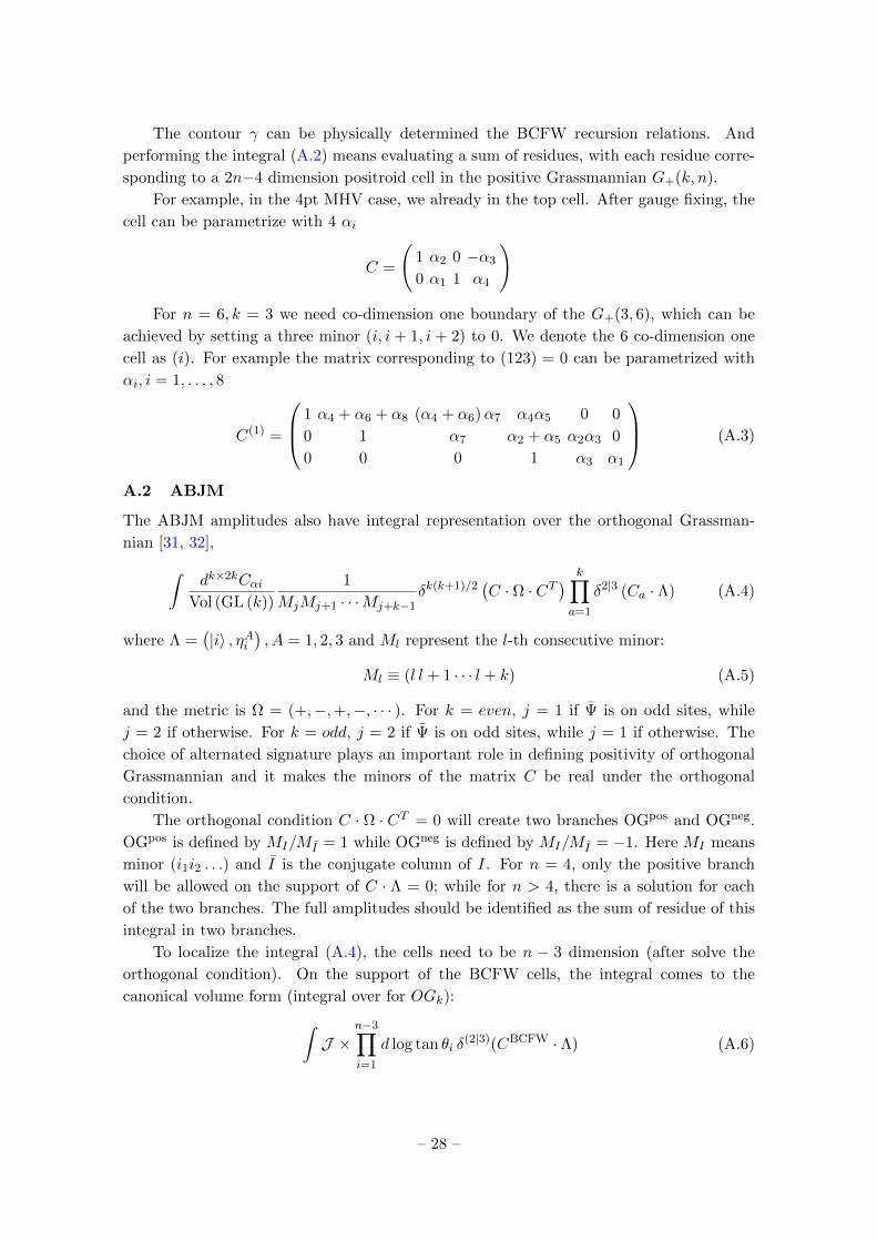
The contour γ can be physically determined the BCFW recursion relations. And

performing the integral (A.2) means evaluating a sum of residues, with each residue corre-

sponding to a 2n−4 dimension positroid cell in the positive Grassmannian G+(k, n).

For example, in the 4pt MHV case, we already in the top cell. After gauge fixing, the

cell can be parametrize with 4 αi

C =

(1 α2 0 −α3

0 α1 1 α4

)For n = 6, k = 3 we need co-dimension one boundary of the G+(3, 6), which can be

achieved by setting a three minor (i, i + 1, i + 2) to 0. We denote the 6 co-dimension one

cell as (i). For example the matrix corresponding to (123) = 0 can be parametrized with

αi, i = 1, . . . , 8

C(1) =

1 α4 + α6 + α8 (α4 + α6)α7 α4α5 0 0

0 1 α7 α2 + α5 α2α3 0

0 0 0 1 α3 α1

(A.3)

A.2 ABJM

The ABJM amplitudes also have integral representation over the orthogonal Grassman-

nian [31, 32],∫dk×2kCαi

Vol (GL (k))

1

MjMj+1 · · ·Mj+k−1δk(k+1)/2

(C · Ω · CT

) k∏a=1

δ2|3 (Ca · Λ) (A.4)

where Λ =(|i〉 , ηAi

), A = 1, 2, 3 and Ml represent the l-th consecutive minor:

Ml ≡ (l l + 1 · · · l + k) (A.5)

and the metric is Ω = (+,−,+,−, · · · ). For k = even, j = 1 if Ψ is on odd sites, while

j = 2 if otherwise. For k = odd, j = 2 if Ψ is on odd sites, while j = 1 if otherwise. The

choice of alternated signature plays an important role in defining positivity of orthogonal

Grassmannian and it makes the minors of the matrix C be real under the orthogonal

condition.

The orthogonal condition C · Ω · CT = 0 will create two branches OGpos and OGneg.

OGpos is defined by MI/MI = 1 while OGneg is defined by MI/MI = −1. Here MI means

minor (i1i2 . . .) and I is the conjugate column of I. For n = 4, only the positive branch

will be allowed on the support of C · Λ = 0; while for n > 4, there is a solution for each

of the two branches. The full amplitudes should be identified as the sum of residue of this

integral in two branches.

To localize the integral (A.4), the cells need to be n − 3 dimension (after solve the

orthogonal condition). On the support of the BCFW cells, the integral comes to the

canonical volume form (integral over for OGk):∫J ×

n−3∏i=1

d log tan θi δ(2|3)(CBCFW · Λ) (A.6)

– 28 –

For the 4-point and 6-point, there is no triangulation of the cells (while for n > 6, cells

start being triangulated). The BCFW cells for n = 4, 6 are the top cells and can be

parameterized as follow

OG4 =

(c 1 s 0

−s 0 c 1

)n=4

, OG6 =

s1+s2s31+s1s2s3

1 c1c21+s1s2s3

0 − c1c3s21+s1s2s3

0

− c1c2s31+s1s2s3

0 s2+s1s31+s1s2s3

1 c2c31+s1s2s3

0c1c3

1+s1s2s30 − c2c3s1

1+s1s2s30 s3+s1s2

1+s1s2s31

(A.7)

here the variables s and c denote sin θ and cos θ. The canonical volume form for n = 4, 6

are

Ω4 = d log tan θi, Ω6 = (1 + s1s2s3)3∏i=1

d log tan θi (A.8)

There is the non-trivial Jacobian factor J6 = 1 + s1s2s3.

The more relevant to us is to consider the reduced SUSY amplitude as we discuss in

the main text (3.26). Here, we show the explicit form of the amplitude in n = 4, 6:

A4 =〈13〉〈12〉〈23〉δ

3(P )δ(4)(Q) (A.9)

A6 = δ3 (P ) δ(4) (q)

p2135

c+25c

+41c

+63

δ(2)

∑p,q,r=2,4,6

〈pq〉 ηr +∑

p,q,r=1,3,5

〈pq〉 ηr

+

p2135

c−25c−41c−63

δ(2)

∑p,q,r=2,4,6

〈pq〉 ηr −∑

p,q,r=1,3,5

〈pq〉 ηr

(A.10)

where

c±rs = 〈r|P135 |s〉 ± 〈r − 2, r + 2〉 〈s− 2, s+ 2〉 (A.11)

B Proof of the relation 〈Y ij〉 = g〈ij〉

Here we prove that brackets in (Y, Y ) space and those in kinematic space are simply related

(with constant g defined in [20]):

〈i j〉 =∑

α,β=1,2

εαβ

(Y ⊥ · Λi

)α (Y ⊥ · Λj

)β=

∑α,β=1,2

k+2∑p,q=1

εαβ

(Y ⊥α,p · Λp,i

)(Y ⊥β,q · Λq,j

)

=

k+2∑p,q=1

(p q)Y ⊥ Λp,iΛq,j

=

k+2∑p,q=1

gεpqr1···rk (r1 · · · rk)Y Λp,iΛq,j

(B.1)

– 29 –

where (p q)Y ⊥ = εαβY⊥α,pY

⊥β,q, which can be rewritten as

g εpqr1···rk (r1 · · · rk)Y =

k∑li=1

g εpqr1···rkεl1l2···lkYl1,r1Yl2,r2 · · ·Ylk,rk

and r1, · · · , rk = 1, 2, · · · p, · · · q, · · · k+2. Then, we can use the identity,

k+2∑p,q=1

k∑li=1

gεpqr1···rkεl1l2···lkYl1,r1Yl2,r2 · · ·Ylk,rkΛp,iΛq,j

=

k+2∑p,q=1

k+2∑ri=1

gεpqr1···rkY1,r1Y2,r2 · · ·Yk,rkΛp,iΛq,j

=g 〈Y ij〉 ,

(B.2)

and similarly for [ij] = g[Y ij]. This completes the proof.

References

[1] E. Witten, “Perturbative gauge theory as a string theory in twistor space,” Commun. Math.

Phys. 252 (2004) 189–258, arXiv:hep-th/0312171 [hep-th].

[2] R. Roiban, M. Spradlin, and A. Volovich, “Tree-level s matrix of yang-mills theory,” Phys.

Rev. D 70 (Jul, 2004) 026009. https://link.aps.org/doi/10.1103/PhysRevD.70.026009.

[3] F. Cachazo and Y. Geyer, “A ’Twistor String’ Inspired Formula For Tree-Level Scattering

Amplitudes in N=8 SUGRA,” arXiv:1206.6511 [hep-th].

[4] F. Cachazo and D. Skinner, “Gravity from Rational Curves in Twistor Space,” Phys. Rev.

Lett. 110 no. 16, (2013) 161301, arXiv:1207.0741 [hep-th].

[5] F. Cachazo, L. Mason, and D. Skinner, “Gravity in Twistor Space and its Grassmannian

Formulation,” SIGMA 10 (2014) 051, arXiv:1207.4712 [hep-th].

[6] F. Cachazo, S. He, and E. Y. Yuan, “Scattering equations and Kawai-Lewellen-Tye

orthogonality,” Phys. Rev. D 90 no. 6, (2014) 065001, arXiv:1306.6575 [hep-th].

[7] F. Cachazo, S. He, and E. Y. Yuan, “Scattering of Massless Particles in Arbitrary

Dimensions,” Phys. Rev. Lett. 113 no. 17, (2014) 171601, arXiv:1307.2199 [hep-th].

[8] F. Cachazo, S. He, and E. Y. Yuan, “Scattering in Three Dimensions from Rational Maps,”

JHEP 10 (2013) 141, arXiv:1306.2962 [hep-th].

[9] F. Cachazo, S. He, and E. Y. Yuan, “Scattering of Massless Particles: Scalars, Gluons and

Gravitons,” JHEP 07 (2014) 033, arXiv:1309.0885 [hep-th].

[10] F. Cachazo, S. He, and E. Y. Yuan, “Einstein-Yang-Mills Scattering Amplitudes From

Scattering Equations,” JHEP 01 (2015) 121, arXiv:1409.8256 [hep-th].

[11] F. Cachazo, S. He, and E. Y. Yuan, “Scattering Equations and Matrices: From Einstein To

Yang-Mills, DBI and NLSM,” JHEP 07 (2015) 149, arXiv:1412.3479 [hep-th].

[12] F. Cachazo, A. Guevara, M. Heydeman, S. Mizera, J. H. Schwarz, and C. Wen, “The S

Matrix of 6D Super Yang-Mills and Maximal Supergravity from Rational Maps,”

arXiv:1805.11111 [hep-th].

– 30 –

[13] J. H. Schwarz and C. Wen, “Unified Formalism for 6D Superamplitudes Based on a

Symplectic Grassmannian,” JHEP 08 (2019) 125, arXiv:1907.03485 [hep-th].

[14] Y. Geyer and L. Mason, “Polarized Scattering Equations for 6D Superamplitudes,” Phys.

Rev. Lett. 122 no. 10, (2019) 101601, arXiv:1812.05548 [hep-th].

[15] N. Arkani-Hamed, Y. Bai, and T. Lam, “Positive Geometries and Canonical Forms,” JHEP

11 (2017) 039, arXiv:1703.04541 [hep-th].

[16] N. Arkani-Hamed, J. L. Bourjaily, F. Cachazo, A. B. Goncharov, A. Postnikov, and J. Trnka,

Grassmannian Geometry of Scattering Amplitudes. Cambridge University Press, 4, 2016.

arXiv:1212.5605 [hep-th].

[17] N. Arkani-Hamed and J. Trnka, “The Amplituhedron,” JHEP 10 (2014) 030,

arXiv:1312.2007 [hep-th].

[18] N. Arkani-Hamed and J. Trnka, “Into the Amplituhedron,” JHEP 12 (2014) 182,

arXiv:1312.7878 [hep-th].

[19] A. Hodges, “Eliminating spurious poles from gauge-theoretic amplitudes,” JHEP 05 (2013)

135, arXiv:0905.1473 [hep-th].

[20] D. Damgaard, L. Ferro, T. Lukowski, and M. Parisi, “The Momentum Amplituhedron,”

JHEP 08 (2019) 042, arXiv:1905.04216 [hep-th].

[21] S. He and C. Zhang, “Notes on Scattering Amplitudes as Differential Forms,” JHEP 10

(2018) 054, arXiv:1807.11051 [hep-th].

[22] Y.-t. Huang and S. Lee, “A new integral formula for supersymmetric scattering amplitudes

in three dimensions,” Phys. Rev. Lett. 109 (2012) 191601, arXiv:1207.4851 [hep-th].

[23] Y.-T. Huang, R. Kojima, C. Wen, and S.-Q. Zhang, “ABJM Amplituhedron,” to appear .

[24] N. Arkani-Hamed, Y. Bai, S. He, and G. Yan, “Scattering Forms and the Positive Geometry

of Kinematics, Color and the Worldsheet,” arXiv:1711.09102 [hep-th].

[25] N. Arkani-Hamed, S. He, and T. Lam, “Stringy canonical forms,” JHEP 02 (2021) 069,

arXiv:1912.08707 [hep-th].

[26] N. Arkani-Hamed, S. He, T. Lam, and H. Thomas, “Binary Geometries, Generalized

Particles and Strings, and Cluster Algebras,” arXiv:1912.11764 [hep-th].

[27] D. Damgaard, L. Ferro, T. Lukowski, and R. Moerman, “Momentum amplituhedron meets

kinematic associahedron,” JHEP 02 (2021) 041, arXiv:2010.15858 [hep-th].

[28] Y. Geyer, A. E. Lipstein, and L. J. Mason, “Ambitwistor Strings in Four Dimensions,” Phys.

Rev. Lett. 113 no. 8, (2014) 081602, arXiv:1404.6219 [hep-th].

[29] S. He, Z. Liu, and J.-B. Wu, “Scattering Equations, Twistor-string Formulas and Double-soft

Limits in Four Dimensions,” JHEP 07 (2016) 060, arXiv:1604.02834 [hep-th].

[30] F. Cachazo, “Resultants and Gravity Amplitudes,” arXiv:1301.3970 [hep-th].

[31] Y.-T. Huang and C. Wen, “ABJM amplitudes and the positive orthogonal grassmannian,”

JHEP 02 (2014) 104, arXiv:1309.3252 [hep-th].

[32] Y.-t. Huang, C. Wen, and D. Xie, “The Positive orthogonal Grassmannian and loop

amplitudes of ABJM,” J. Phys. A47 no. 47, (2014) 474008, arXiv:1402.1479 [hep-th].

[33] N. Arkani-Hamed, H. Thomas, and J. Trnka, “Unwinding the Amplituhedron in Binary,”

JHEP 01 (2018) 016, arXiv:1704.05069 [hep-th].

– 31 –

[34] L. Ferro, T. Lukowski, and R. Moerman, “From momentum amplituhedron boundaries to

amplitude singularities and back,” JHEP 07 no. 07, (2020) 201, arXiv:2003.13704

[hep-th].

[35] N. Arkani-Hamed, J. Bourjaily, F. Cachazo, and J. Trnka, “Unification of Residues and

Grassmannian Dualities,” JHEP 01 (2011) 049, arXiv:0912.4912 [hep-th].

[36] Y.-t. Huang, “Non-Chiral S-Matrix of N=4 Super Yang-Mills,” arXiv:1104.2021 [hep-th].

[37] H. Elvang, Y.-t. Huang, C. Keeler, T. Lam, T. M. Olson, S. B. Roland, and D. E. Speyer,

“Grassmannians for scattering amplitudes in 4d N = 4 SYM and 3d ABJM,” JHEP 12

(2014) 181, arXiv:1410.0621 [hep-th].

[38] T. Lukowski, M. Parisi, and L. K. Williams, “The positive tropical Grassmannian, the

hypersimplex, and the m=2 amplituhedron,” arXiv:2002.06164 [math.CO].

[39] M. Parisi, M. Sherman-Bennett, and L. Williams, “The m=2 amplituhedron and the

hypersimplex: signs, clusters, triangulations, Eulerian numbers,” arXiv:2104.08254

[math.CO].

[40] D. Damgaard, L. Ferro, T. Lukowski, and R. Moerman, “Kleiss-Kuijf Relations from

Momentum Amplituhedron Geometry,” JHEP 07 (2021) 111, arXiv:2103.13908 [hep-th].

[41] Z. Bern, J. J. M. Carrasco, and H. Johansson, “New Relations for Gauge-Theory

Amplitudes,” Phys. Rev. D 78 (2008) 085011, arXiv:0805.3993 [hep-ph].

[42] T. Bargheer, S. He, and T. McLoughlin, “New Relations for Three-Dimensional

Supersymmetric Scattering Amplitudes,” Phys. Rev. Lett. 108 (2012) 231601,

arXiv:1203.0562 [hep-th].

[43] Y.-t. Huang and H. Johansson, “Equivalent D=3 Supergravity Amplitudes from Double

Copies of Three-Algebra and Two-Algebra Gauge Theories,” Phys. Rev. Lett. 110 (2013)

171601, arXiv:1210.2255 [hep-th].

[44] N. Arkani-Hamed, F. Cachazo, C. Cheung, and J. Kaplan, “A Duality For The S Matrix,”

JHEP 03 (2010) 020, arXiv:0907.5418 [hep-th].

– 32 –