THE NATIONAL INSTITUTE MODEL - simdynamics.org manual.pdf · THE NATIONAL INSTITUTE MODEL FOR...

THE NATIONAL INSTITUTE MODEL

FOR LIFETIME INCOME

DISTRIBUTIONAL ANALYSIS, LINDA This manual provides practical guidance in the use of LINDA, a dynamic

microsimulation model that projects a reference population cross-section through time, subject to endogenous savings and labour supply decisions.

User Manual version 3.11

J. van de Ven 18 July, 2016

1 | P a g e

The National Institute Lifetime INcome Distributional Analysis model LINDA

User Manual

Table of Contents 1. Introduction .................................................................................................................................... 4

2. Model set-up on a dedicated workstation ...................................................................................... 6

System requirements .......................................................................................................................... 6

Loading the model onto a new computer .......................................................................................... 6

Extracting base data from the Wealth and Assets Survey .................................................................. 8

Creating a simulation base .................................................................................................................. 8

Using MPI integrations ........................................................................................................................ 9

Setup ............................................................................................................................................. 10

Running the model using MPI ....................................................................................................... 10

3. Using the model on a cloud service .............................................................................................. 11

Cloud computing providers and LINDA ............................................................................................. 11

Step 1: Set-up a stand-alone simulation on a local computer .......................................................... 12

Local system requirements ........................................................................................................... 12

Model set-up on the local computer ............................................................................................ 12

Step 2: Start a cloud instance ........................................................................................................... 14

Step 3: Upload the stand-alone model onto the cloud instance ...................................................... 25

Step 4: Run the model on the cloud ................................................................................................. 28

Step 5: Download results to the local computer .............................................................................. 29

Step 6: Terminate the instance ......................................................................................................... 29

Step 7: Analyse model output – creating a new simulation base ..................................................... 30

Final points of note ........................................................................................................................... 30

4. Altering Parameters ...................................................................................................................... 31

FORM 0: SIMULATION TASK ............................................................................................................. 32

FORM 1: KEY PARAMETERS ............................................................................................................... 34

FORM 2: ANALYSE EXISTING SIMULATION ....................................................................................... 37

FORM 3: FERTILITY ASSUMPTIONS ................................................................................................... 40

FORM 4: SELECTED EMPLOYMENT PARAMETERS ............................................................................ 41

FORM 5: SELECTED DISABILITY PARAMETERS .................................................................................. 42

2 | P a g e

FORM A1: INCOME TAX AND NATIONAL INSTURANCE (2010/11) ................................................... 44

FORM A2: TAX CREDITS – WORKING LIFETIME ................................................................................. 45

FORM A3: HOUSING RELATED BENEFITS .......................................................................................... 46

FORM A4: BENEFITS FOR NON-DISABLED ......................................................................................... 47

FORM A4: DISABILITY BENEFITS ........................................................................................................ 48

FORM A6: AGE THRESHOLDS ............................................................................................................ 49

FORM A7: UNIVERSAL CREDIT .......................................................................................................... 50

FORM A8: INDIRECT TAXATION ........................................................................................................ 51

FORM C1: STATE CONTRIBUTORY PENSIONS ................................................................................... 52

FORM C2: NON-PENSION WEALTH ................................................................................................... 53

FORM C3: PRIVATE PENSIONS .......................................................................................................... 54

FORM C4: VARIATION OVER PRIVATE PENSION ELIGIBILITY ............................................................ 56

FORM C5: PRIVATE PENSIONS (cont.) ............................................................................................... 57

FORM C6: ESCALATION ..................................................................................................................... 58

FORM C7: SELF-EMPLOYMENT ......................................................................................................... 59

FORM C8: EDUCATION ...................................................................................................................... 60

FORM D1: SHORT-RUN ANALYSIS ..................................................................................................... 61

FORM D4: ANALYSIS OF TAX FUNCTION ........................................................................................... 62

FORM Z: RUN MODEL ....................................................................................................................... 63

5. Running the model on a local computer....................................................................................... 64

Stacking simulation counterfactuals ................................................................................................. 64

6. Simulation Output ......................................................................................................................... 66

Benefit unit level micro-data ............................................................................................................ 66

Default summary statistics ............................................................................................................... 68

High-level summary statistics - hi_level_statistics.xls .................................................................. 68

Optional summary statistics ............................................................................................................. 70

High level analysis of population cross-sections and birth cohorts .............................................. 70

Poverty statistics ........................................................................................................................... 70

Decile-level summary statistics for population cross-sections and birth cohorts ........................ 70

7. Best Practice Methods of Use ....................................................................................................... 73

Step 1: specify policy parameters ..................................................................................................... 73

Checking differences with base simulation .................................................................................. 73

Validating the tax function ............................................................................................................ 73

Example ......................................................................................................................................... 74

3 | P a g e

Step 2: run model and generate output ........................................................................................... 81

Example ......................................................................................................................................... 81

Step 3: think about likely incentive effects ....................................................................................... 82

Example ......................................................................................................................................... 82

Step 4: analyse model output ........................................................................................................... 82

High level analysis ......................................................................................................................... 82

Detailed statistical analysis ........................................................................................................... 82

What to do when results do not conform to expectations .......................................................... 83

Example ......................................................................................................................................... 83

Step 5: package output ..................................................................................................................... 86

8. Adjusting the Program Code ......................................................................................................... 87

Programming basics .......................................................................................................................... 87

Basic Code Structure ..................................................................................................................... 87

Common programming steps ....................................................................................................... 89

Programming a new Tax and Benefits Regime ................................................................................. 92

Organisation of the Tax and Benefits Code .................................................................................. 92

Introducing user-defined tax schemes ......................................................................................... 93

Adjusting number of tax outputs .................................................................................................. 97

Appendix A: End User License ............................................................................................................... 99

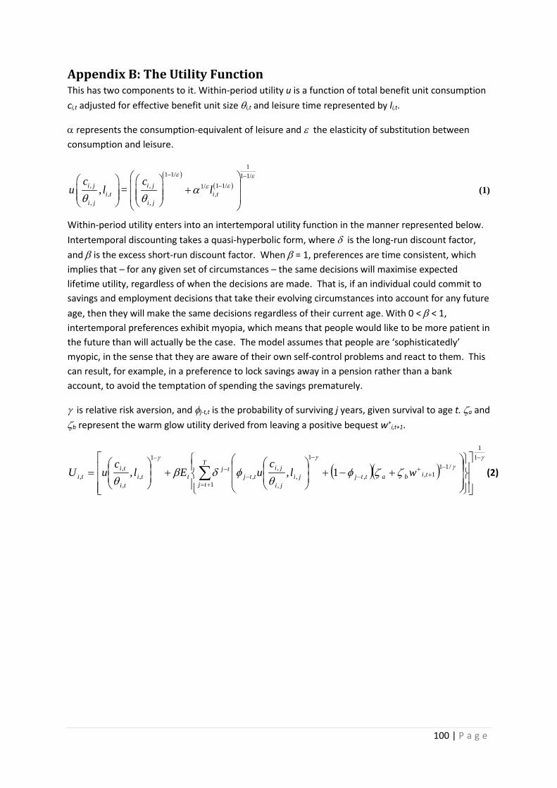
Appendix B: The Utility Function ........................................................................................................ 100

4 | P a g e

1. Introduction This manual describes use of the National Institute's Lifetime INcome Distributional Analysis model, LINDA, which is designed to explore the effects of changes to the tax and benefits structure on household circumstances through time. The model generates panel data for the evolving population cross-section, and a series of summary statistics for each considered policy environment.

LINDA is complementary to other analytical approaches that are now in use. Current large scale microsimulation models are able to provide detailed information regarding the immediate financial implications of policy change. However, such models are not well adapted to consider how savings, employment and consumption can be expected to adapt to altered financial incentives. Econometric analyses can go some way to filling in this missing detail, but not where uncertainty is likely to influence decision making. LINDA is specifically designed to explore savings and employment responses to policy change in context of important aspects of uncertainty that individuals face. The cost of this approach is that it is unable to reflect the degree of detail that is commonly taken into account by the two alternative analytical approaches that are referred to above. Thus, a thorough basis for balanced policy advice is best achieved at present by considering the same issue from alternative analytical perspectives.

LINDA is comprised of a series of Excel files that describe model parameters, and a central executable program that undertakes all of the requested analyses. Alteration of the model parameters is facilitated through an Excel “front-end”, via a series of “user forms”. One purpose of this manual is to describe how to use this Excel front-end. But before we move on to that, it is worth describing at a very high level of detail how the model works.

The model starts from cross-sectional data for the benefit units of a sample of reference adults drawn from the Wealth and Assets Survey. As such, use of the model is limited to individuals who have been granted access to the Wealth and Assets Survey microdata.1 A benefit unit is defined as one or two adults (living together as a couple) plus any dependent children living with them. The user is first directed to run a simulation that projects the circumstances for the reference population cross-section back through time, and the evolving population cross-section forward through time. This base simulation allows the model to describe the complete life-history of each adult represented in the reference cross-section. The micro-data generated by the model are saved by the model, and used as the “base” data from which subsequent policy-specific projections are made. It is possible to update the “base” data used by the model at any time, as is described later in this manual.

A simulation for a given policy environment typically involves 3 stages. 1) Specify model parameters through an Excel spread sheet. 2) Run the executable program, which automatically loads the model parameters, projects associated panel data starting from the prevailing simulation “base” (output in a standard format, csv), and calculates a set of associated summary statistics (output to Excel). 3) Analyse the model output.

Although users are unable to access the source code of the main executable program, they are able to alter in any way that they like the auxilliary files that implement taxes and benefits in the model.2

1 See the UK Data Archive, Catalogue number 6415; “Wealth and Assets Survey, Waves 1-2, 2006-2010: Special Licence Access”. 2 Source code for selected aspects of the model is available from the author upon request.

5 | P a g e

This manual also provides a brief description of how the tax and benefit code considered by the model can be altered.

LINDA is at the prevailing technological frontier. Nevertheless, it is important to recognise the model’s limitations from the very outset. This is especially important, because the style of output generated by LINDA can result in mis-conceptions concerning the accuracy of projections; for example, consumption is projected by the model for each family unit down to the last pence (and even beyond that), giving the illusion of a very high degree of accuracy. Technical and theoretical limitations, however, mean that any projection of the future that we make today should not be interpreted as either a forecast or a prediction. Rather, such projections are useful because they reveal the logical implications of alternative policy environments that could only otherwise be guessed at, given a set of explicit (albeit, unavoidably imperfect) assumptions concerning how the future will evolve.

This manual is divided into seven sections. Section 2 describes how the model should be set-up for the first time on a dedicated workstation, which includes use of the Excel front-end. Workstations tend to be expensive investments, at least for independent researchers. The model has consequently been adapted to run on cloud computing services, which permit individual simulations to be run at very little cost. Section 3 describes how to set the model up to run on a cloud computing service. Section 4 describes how to use the Excel front-end, which is designed to guide a user through adjustment of selected model parameters. Section 5 describes the output generated by the model. Section 6 provides an overview of how to use the model to conduct policy analyses. Section 7 provides some pointers for those interested in altering the tax and benefit programing code.

Beyond this manual, a wide range of resources exist to aid in the use of the model. These resources, which include access to aspects of the underlyin model code, video tutorials, and a user forum, can all be accessed at the dedicated website: www.simdynamics.org.

http://www.simdynamics.org/

6 | P a g e

2. Model set-up on a dedicated workstation

System requirements LINDA is designed to operate on desktop workstations that use Intel processors and the Microsoft Windows operating system. We recommend minimum system specifications of a 64 bit operating system, computing processor(s) with at least 6 physical cores, 32GB of RAM, and 1TB of hard disk space.3 Microsoft Excel is required to generate parameter alternatives and analyse summary statistics reported by the model. Stata is required to run a file that we have written to extract the required micro-data from the Wealth and Assets Survey, and supplementary routines we have written to aid analysis of generated microdata. Users who intend to alter the tax and benefits structure beyond simple parameter adjustments, will also require Intel Fortran Studio XE or Intel Parallel Studio XE. A computer monitor not less than 19” in diagonal dimension is also required.

Loading the model onto a new computer The model is delivered as a single install.exe file. Double click on the file, and work through a standard set of install options. The user license agreement is included in Appendix A to this document. Minor issues to note include:

• The model can be installed onto any directory of your choosing, subject to the limitation that the directory name should not include the character “.” Note that the installer will add “NIESR\SIDD” to a folder that you navigate to through the installer. You should delete this added directory extension if desired.

• The installer adds SIDD.exe to the Windows “Programs and Features” list. You can uninstall the model either through the “Programs and Features” list, or by simply deleting the model’s install directory.

o The uninstall feature supplied with the model will not delete any files or folders that the user has created within the model’s subdirectory. These should be deleted manually if desired.

• Model updates are delivered in the same fashion as the full model install. If an update is installed in the same directory as the original model, then it will over-write all pre-existing model files except those that have been generated by the user. This means that all of the simulations that you have generated via a previous version of the model will not be deleted when you up-date the model.

The installer creates four subdirectories: DOCUMENTATION, FORTRAN, MODEL, and STATA.

• The DOCUMENTATION subdirectory includes the model’s user manuals. • The FORTRAN subdirectory includes the programming code for the TAX routines that are

provided with the model. • The MODEL subdirectory includes all of the files that are required to run the model.

3 The model is delivered on the assumption that you have a 64 bit operating system. Please contact the NIESR if you require files to run on a 32 bit system. Note also that these minimum system requirements are for the base model specification, and are not sufficient for every feasible model specification. Please contact NIESR for further assistance.

7 | P a g e

• The STATA subdirectory includes a set of Stata files that we have written as an introduction to aiding analysis of the micro-data that are generated by the model.

The MODEL subdirectory contains three subdirectories in addition to a set of model files. The subdirectory ANALYSIS_FILES contains a set of Excel files that are used by the model’s in-built analysis routines, and an additional subdirectory that stores some related statistics. The subdirectory BASE_FILES contains a separate subdirectory for each "base" specification that you create with the model, in which files that are required for the respective base specification are stored (discussed in the section concerned with “FORM 0” that we return to below). The subdirectory SIMULATIONS will contain a separate subdirectory for each simulation that you run, in which are stored the panel data generated by the model, model parameters, and excel simulation output.

Please follow these steps when installing the model on a new computer:

1. Run the file setup.exe, as referred to above

USERS WITH FORTRAN PROCEED TO STEP 2 – ALL OTHERS SKIP TO THE SUBSECTION ENTITLED “Extracting base data from the Wealth and Assets Survey” ON THE NEXT PAGE

2. In the FORTRAN subdirectory, open up the TAXES subdirectory, and double-click on TAXES.sln

a. This should open the Visual Studio program environment 3. If you can see the “solution explorer” window, then select the “TAXES” box under the

“Solution ‘TAXES’” project a. If you cannot see the “solution explorer” window, then open it through the “View”

drop-down menu 4. In the “Project” drop-down menu at the top of Visual Studio, select “Properties” 5. In the “Configuration” drop-down menu select “All configurations” 6. In the “Platform” drop-down menu select “All platforms” 7. Under “Configuration Properties”, select the “General” category 8. Against the “Output Directory”, replace “C:\MyFiles\MODEL_LAB\MODEL\” with the file

location that you have saved the model into 9. Under “Configuration Properties”, select the “Debugging” category 10. Against “Command”, enter the location of the file “SIDD.exe”; eg:

“C:\MyFiles\MODEL_LAB\MODEL\SIDD.EXE” 11. Against “Working Directory”, enter the same text as under (8) 12. Press the “Apply” button, and then the “Ok” button 13. Under the “File” drop-down menu select “Save All” 14. Under the “Build” drop-down menu select “Configuration Manager” 15. Under the “Active Solution Configuration” select “release” 16. Under the “Active Solution Platform” select “x64” and press the “Close” button4 17. Under the “Build” drop-down menu select “Rebuild Solution”

4 If running a 32 bit environment then select “Win32” here.

8 | P a g e

You should then see some text like, indicating that everything has worked:

1>------ Rebuild All started: Project: TAXES, Configuration: release x64 ------ 1>Deleting intermediate files and output files for project 'TAXES', configuration 'release|x64'. 1>Compiling with Intel(R) Visual Fortran Compiler XE 15.0.4.221 [Intel(R) 64]... 1>2_global.F90 1>UK_3.F90 1>UK_4.f90 1>1_TaxTools.f90 1>UK_2.F90 1>AUS_1.f90 1>IT_1.f90 1>IE_1.F90 1>UK_1.F90 1>0_app_taxes.f90 1>Linking... 1> Creating library C:\MyFiles\MODEL_LAB\MODEL\TAXES.lib and object C:\MyFiles\MODEL_LAB\MODEL\TAXES.exp 1> 1>Build log written to "file://C:\MyFiles\MODEL_LAB\FORTRAN\TAXES\x64\release\BuildLog.htm" 1>TAXES - 0 error(s), 0 warning(s) ========== Rebuild All: 1 succeeded, 0 failed, 0 skipped ==========

Extracting base data from the Wealth and Assets Survey As noted in the introduction, the model starts with data reported by the Wealth and Assets Survey (WAS) for a population cross-section of reference adults. A Stata program (e.g. derive_WAS 2011.do) is provided in the model subdirectory “\MODEL\base_files\” to extract and format the WAS data, ready for importing into the model. Please open the file derive_WAS.do, edit the directory locations as indicated by comments at the top of the file, and run it to generate the base dataset.

Creating a simulation base As noted in the introduction, the model starts with data reported by the Wealth and Assets Survey for a population cross-section of reference adults. The model parameters have been calibrated to match the model to a wide range of summary statistics calculated from survey data sources, with the calibration structured around the year in which the reference population was observed (see van de Ven and Lucchino, 2013, for details). The model comes packaged, ready to project the circumstances of the population cross-section forward and backward through time, to build up a complete life history for each reference individual. It is recommended that this be done, and that the associated data should be defined as the “base” for subsequent simulations. This can be done by following steps 18 to 28 below.

18. Open the MODEL subdirectory, and then open “job file.xls” a. note that a “Security Warning” may appear in Excel if macros have been disabled

19. Ensure that you allow macros to work in Excel a. please ask your system administrator if you require assistance with this

20. Press ALT+F8 21. Select “SIDD” and press the RUN button 22. Press the “RUN EXISTING JOB FILE” button

a. A warning message may appear if the model identifies the potential for insufficient system memory. If system memory is a problem, then it is possible to proceed using cloud computing services, as discussed in Section 3 of this manual

9 | P a g e

The current base version of the model runs in around 5 hours – the associated simulation creates a new set of base data for analysis, using the full model specification.

23. Re-open “job file.xls” 24. Press ALT+F8 25. Select “SIDD” and press the RUN button 26. Enter “base_2011” into the text-box with the title “name of run to adopt as new base” 27. Enter “base_2011” into the text-box with the title “directory name for new base” 28. Press the “CONVERT RUN TO NEW BASE” button

Excel will then work away for a short while, after which you should receive a message confirming that the new base has been created. If you look in the BASE_FILES subdirectory, you should now see a new subdirectory with the name “base_2011”, which includes all of the files defining the base simulation specification.

To test that the model set-up has been successfully completed:

29. Re-open “job file.xls” a. This file has been changed since step (23), so that it now references the new base

model directory by default. 30. Press ALT+F8 31. Select “SIDD” and press the RUN button 32. Press the “SET UP NEW SIMULATION” button 33. Type “test” in the text-box with the title “Simulation Name” 34. Press the “ENTER” button 35. Tick the box to direct the model to calculate “statistics for equivalised income deciles” 36. Tick the box to indicate that “comparative statistics with the population base” should be

evaluated 37. Press the “ENTER AND RUN” button 38. Press the “LAUNCH MODEL” button

The model should then run through once again, in around 1.5 hours. This time, however, the simulations will project only forward through time, taking the population characteristics back in time from the base specification. When the model is complete, please open the analysis_dec.xls file that is created in the “test” simulation directory, and check that all of the statistics reported in the “differences with base” sheet are close to zero.

Using MPI integrations If the model is run on a computer with two or more physical processors5, as is currently available in workstations and a feature of HPC (High Performance Computing) clusters, then substantial reductions in computation time can be realised by taking advantage of the MPI integration that has been built into the model. It is necessary to perform a number of additional steps to set the model up for use with MPI integrations.

5 A ‘physical processor’ refers to a Central Processing Unit or CPU. Each CPU may include multiple (physical) computing ‘cores’

10 | P a g e

Setup The Intel MPI run-time libraries must be installed to take advantage of MPI integrations. These run-time libraries are freely available from the Intel website, and a copy of the associated install program is provided in the Intel subdirectory included with the model.

After the Intel MPI libraries are installed, it is necessary to register a user-name and password with the MPI libraries, which are encrypted and stored by the system to permit the creation of MPI processes. This is done by opening a Command Prompt window (type cmd in the windows search box), and typing “mpiexec -register”.

Running the model using MPI Two additional things are then required each time you want to run the model using MPI integrations. First, the prevailing model parameters need to be TRANSLATED for suppressing communications with Excel. To do this:

1. Open the MODEL subdirectory, and then open “job file.xls” 2. Ensure that you allow macros to work in Excel

a. please ask your system administrator if you require assistance with this 3. Press ALT+F8 4. Select “TRANSLATE” and press the RUN button

A series of Excel macros will then run through, ending in a message to indicate that model parameters have been successfully translated for reading in without recourse to Excel.

Secondly, open a Command Prompt window, navigate to the directory that the model is stored in (by typing cd XXX, where “XXX” is replaced by the location of the main model directory; e.g. “C:\MyFiles\MODEL_LAB\MODEL”), and type:

mpiexec -n X sidd

and hit the RETURN key. “X” here defines the number of MPI processes, and should be replaced by the desired figure. As a general rule, set X to the number of CPU’s in your system. You should then see some output like the following:

The second line of output should indicate that the number of MPI tasks is set to “X”, after which “X” lines should appear indicating the index and computer name of each MPI task.

11 | P a g e

3. Using the model on a cloud service LINDA is computationally intensive, and as such can impose a heavy demand on computing resources. The model has consequently been adapted to take advantage of modern computing technology, including the possibility of running it entirely on a cloud computing service. Running the model on a cloud service has the distinct advantage that it permits the user to rent access to specialist computing services, which they may not need on a day-to-day basis. The model is designed to take advantage of both “shared memory” systems (as present in a single personal computer, workstation, or computational “instance” discussed below), and “distributed memory” systems (as present in High-Performance Computing, or supercomputer, clusters). This section walks through the steps required to run the model on a single computation “instance” in a cloud service. How to establish and run the model on a computer cluster (comprised of multiple “instances”) is beyond the scope of this manual.

Cloud computing providers and LINDA There are currently a large number of cloud computing providers, consistent with an industry-wide view that cloud computing is likely to account for an increasing share of computational demand in the future. Each provider has its own strengths and weaknesses, which evolve at a rapid pace. This section refers to services provided by Amazon through its Elastic Compute facility (EC2), though it could just as easily have referenced Google’s Compute Engine, or Microsoft’s Azure. The user is advised to seek out the option that best suits their needs.

Cloud computing services are organised around “instances”, which can be thought of as individual (virtual) computers. Each instance is assigned an explicit set of compute resources, including “virtual central processing units”, vCPUs, memory, RAM, and physical disk space. Costs are typically charged per minute or hour, and vary with the scale of the resources that are rented.

It is possible to access instances individually, or as a group. A group of instances that has been organised to work together is sometimes referred to as a “cluster”. Individual instances are typically limited to the specifications of a prevailing high-end desktop workstation. Clusters, in contrast, offer potentially unlimited resources. While the number of vCPUs currently accommodated on an instance is limited to 40, clusters comprised of up to 156,000 vCPUs (cores) have been used. In this regard, it is useful to bear in mind that the computational time of a simulation is generally inversely proportional to the number of cores. Hence, a problem that would take a week to compute on a single vCPU, would take 4.2 hours to compute on a 40 vCPU instance, and just under 4 seconds to compute on a 156,000 vCPU cluster.

An important point to note is that LINDA is currently limited to accessing a single instance at any one time. The current description is consequently limited to discussion of how to launch and use a single instance, noting that an additional layer of complexity is associated with the establishment and use of a cluster.

Most cloud computing services that currently exist supply instances with minimal pre-installed software. There are two ways to use LINDA in context of these software limitations.

In the first alternative, a dedicated instance can be started, and the user can load all of the software required to run the model onto the instance. As all data loaded onto an instance are lost when an instance is terminated, this approach lends itself to renting an instance for the entire duration of an

12 | P a g e

analysis of interest. In this case, the model set-up would proceed in a similar fashion to that described in Section 2 for a dedicated workstation.

The second alternative involves renting an instance only for the duration of a single simulation. In this case, it is necessary to:

1) Use a local computer to set up a stand-alone model specification that is designed to minimise software pre-requisites

2) Start a cloud instance 3) Upload the stand-alone model specification onto the instance 4) Run the model specification 5) Download results to the local computer 6) Terminate the instance 7) Analyse results on the local computer

The remainder of this section walks through each of the seven steps that are listed here.

Step 1: Set-up a stand-alone simulation on a local computer

Local system requirements Setting-up a stand-alone model specification requires a computer with any operating system, a monitor not less than 19” in diagonal dimension, an internet connection (to access the cloud), and two pieces of off-the-shelf software. Microsoft Excel is needed to generate parameter alternatives and analyse summary statistics. Stata is required to run a file that we have written to extract the required micro-data from the Wealth and Assets Survey, and to use supplementary routines that we have written to aid analysis of simulated microdata. Users who intend to alter the tax and benefits structure beyond simple parameter adjustments will also require a 64-bit Microsoft Windows operating system, and Intel Fortran Studio XE or Intel Parallel Studio XE.

Model set-up on the local computer Setting-up the model on a local computer is described at length in Section 2. Please follow the directions outlined in the three subsections of Section 2 preceding the subheading “Creating a simulation base”.

In common with the procedure of setting up a model on a dedicated workstation, we recommend that analysis start by setting up a base simulation. This base simulation projects data forward and backward through time using a base parameter specification, building up a description for the complete life-course of individuals present in a reference population cross-section. The model parameters necessary to undertake this simulation come pre-packaged with the model. The remainder of this section describes how to run this base simulation on Amazon’s EC2. Please note that a similar set of steps to those described below is required to run subsequent simulations.

A stand-alone specification for the model using the pre-packaged parameters can be generated via the following steps:


a. please ask your system administrator if you require assistance with this

13 | P a g e

7. Press ALT+F8 8. Select “TRANSLATE” and press the RUN button

A series of Excel macros will then run through, ending in a message to indicate that model parameters have been successfully translated for reading in without recourse to Excel. The model is now ready for copying to an instance on the cloud.

Individuals who have access to a 64bit Windows operating system can now use the model on their local machine to generate useful statistics for determining the cloud resources that they need. This can be done by following these steps:


a. please ask your system administrator if you require assistance with this 3. Press ALT+F8 4. Select “SIDD” and press the RUN button 5. Press the “NEW SIMULATION FOR UK” button 6. Type “temp” in the text box next to “simulation name” 7. Press the “ENTER” button 8. Select the checkbox next to “generate advisory statistics…” 9. Press the “ENTER AND RUN” button 10. Press the “LAUNCH MODEL” button

You should then see output similar to the following:

The first line of output following “Running job temp” indicates that selecting a single vCPU instance will solve the utility maximisation problem in approximately 37.8 hours, and the full simulation

14 | P a g e

output in approximately 38.5 hours. Note that the time taken to evaluate the utility maximisation problem declines approximately proportionally with the number of vCPUs, while the time taken for the remainder of the simulation is broadly unaffected by the number of vCPUs. Hence, the above statistics imply that selecting a cloud instance with 10 vCPUs should run in approximately 4.5 (= 3.78 + 0.7) hours. The model output also indicates that the problem will require approximately 19GB of RAM, and 8GB of physical disk space.

Step 2: Start a cloud instance Amazon Web Services (AWS) offer a very wide variety of cloud computing services. Users should refer to the website https://aws.amazon.com/ for full details concerning how to set-up a user account, and what facilities are on offer.

Like most cloud computing options that are currently available, there are no sign-on costs for AWS, no fixed costs, and no mandatory contract periods; you only pay for what you use. The description here is limited exclusively to the steps involved in initialising and running the model on EC2 available through AWS, assuming that an account has been set up.

1) Sign in to the AWS console using your account credentials.

https://aws.amazon.com/

15 | P a g e

2) Select EC2 from the main menu

16 | P a g e

3) Select “Launch an instance” a. We recommend using a “on-demand” instance

17 | P a g e

4) Select an Amazon Machine Image (AMI) that has Microsoft Windows Server installed. a. Note: do not select a server with SQL included, as SQL is not needed by the model

and the associated AMIs are more expensive to rent

e.g. use this one

not this one

18 | P a g e

5) Select an instance type a. we typically focus on the compute optimised options, b. Ensure that there are sufficient vCPUs (A) and RAM (B) c. press Next

A B

19 | P a g e

6) Default instance details are fine for us, click next

20 | P a g e

7) Add sufficient storage for the simulation. a. The model advised that we require at least 8GB of storage space for the simulation.

The basic system supplied with the instance takes up just over 21GB and the model takes up 0.5 GB. The model will return an error code if it runs out of storage space, and require re-launching. We consequently suggest that at least 10GB of storage beyond the very minimum is requested. In our context, this is 40GB (=21 + 8 + 0.5)

21 | P a g e

8) There is no need to tag our instance – press next

22 | P a g e

9) Edit security groups, and press review and launch

23 | P a g e

10) Create a new key pair, download the key, and launch a. You start paying for the instance from the time that you press the Launch button.

24 | P a g e

11) Go to the instances monitoring page, and wait for the new instance to initialise

25 | P a g e

Step 3: Upload the stand-alone model onto the cloud instance 10) Put all of the files in the \MODEL subdirectory into a zipped folder 11) Connect to your instance once it is ready:

26 | P a g e

12) Use the key pair that was created at step 8 to obtain a password:

27 | P a g e

13) Store the password for future reference and download remote desktop file:

14) Open the remote desktop download, and connect using the password obtained in the preceding step.

15) After a moment for the initialisation, you should be able to see the desktop of your instance. 16) Copy the zip folder with the model onto your instance.

a. Note that the time this takes will depend upon the speed of your internet connection

b. Note also, that you should not copy or paste anything on your computer while the download is taking place, or it may fail

28 | P a g e

Step 4: Run the model on the cloud 17) When the download is complete, extract the model from the zip folder using Windows

explorer to a folder of your choosing on the instance 18) Double click on SIDD.exe in the \MODEL subdirectory on the instance.

The model should now run through to completion, providing a message when it is complete

29 | P a g e

Step 5: Download results to the local computer 19) Put all of the files in the “\MODEL\simulations\2011_base” subdirectory on your instance

into a zip folder, including the “anals” and “long_file” subdirectories, but omitting the “grids” subdirectory

20) Copy this zip file and paste it to your local computer 21) Extract the files and folders to a “2011_base” folder in your “\MODEL\simulations”

subdirectory.

Step 6: Terminate the instance 22) You stop paying for the instance when the instance is terminated:

30 | P a g e

Step 7: Analyse model output – creating a new simulation base 1. Re-open “job file.xls” 2. Press ALT+F8 3. Select “SIDD” and press the RUN button 4. Enter “base_2011” into the text-box with the title “name of run to adopt as new base” 5. Enter “base_2011” into the text-box with the title “directory name for new base” 6. Press the “CONVERT RUN TO NEW BASE” button

Excel will then work away for a short while, after which you should receive a message confirming that the new base has been created. If you look in the BASE_FILES subdirectory, you should now see a new subdirectory with the name “base_2011”, which includes all of the files defining the base simulation specification.

Final points of note Up-load and down-load times can be non-trivial when working with the model. It may be possible to economise these costs by storing data in the cloud with your provider.

Another point that may help to economise data up-load and down-load times concerns the information that the model requires to run a simulation. In this case, the model requires all files in the \MODEL subdirectory, including its child subdirectories, except the following:

• No subdirectories are required under the “MODEL\simulations” directory • The model only requires the files in the “MODEL\base_files\XXX” subdirectory, where XXX

refers to the name given to your prevailing simulation base (base_2011 in the above example). All other subdirectories in “MODEL\base_files\” can be omitted.

31 | P a g e

4. Altering Parameters Most of the key model parameters are stored in the spread sheet “job file.xls”. Altering this file name may prevent the main executable file SIDD.exe from locating the model parameters.6 “Job file.xls” is comprised of a number of worksheets. The parameters which drive the model are present in the worksheet input. Parameter values of the base simulation are stored in the sheet inputA. Expert users can make changes directly to the parameters described in the input worksheet, without recourse to the user front-end. Alternatively the front-end system of forms that is included with the spread sheet can be used to alter a selected set of model parameters. Differences between the data stored in the input and inputA sheets are identified by 1s in the check sheet. Any other sheets included in “job file.xls” are beyond the scope of this manual, and should not be altered by the user.

To use the front-end, users should open “job file.xls” and run the macro “SIDD”, visible in the Tools/Macros window (Alt+F8). This displays Form 0.

6 The only exception is in the case when the user would like to “stack” a series of simulations for consecutive (automated) execution. In this case, the “job file” associated with each alternative simulation should be numbered in their order or execution – e.g. “job file1.xls”, “job file2.xls”, “job file3.xls”…

32 | P a g e

FORM 0: SIMULATION TASK

Form 0 offers the user a series of alternative options for running LINDA.

Setting up a New Simulation

This function allows the user to define and run a new simulation from scratch. Pressing the “NEW SIMULATION FOR UK” button will lead to a series of alternative user forms, which are designed to guide the user through the process of altering a selected set of model parameters. The related forms are described below.

Run Existing Job File

An existing job specification (as described by the parameters on the existing input sheet) can be run by clicking the “RUN EXISTING JOB FILE” button. The name of the simulation will be auto-populated with whatever name exists in cell A2 of the current input sheet. The user may alter this name to an alpha-numeric combination of their choosing. The model will then run, and save all associated results into a subdirectory with the name given to the simulation.

Analysing the Tax Function

It is often useful to “eyeball” the influence of simulated taxes and benefits on benefit units. The model includes two analysis routines for this purpose, which can be accessed by pressing the

33 | P a g e

“ANALYSE TAX FUNCTION” button. The associated analysis routines are described under “Form D4” later in this manual.

Analyse Existing Simulation

The model permits a series of supplementary analyses to be run after a given simulation is complete. Pressing the “ANALYSE EXISTING SIMULATION” button will open a new form that allows the user to choose which additional analyses will be performed. This alternative is returned to under “Form 2” below.

Convert Run to New Base

As discussed in the introduction, the model projects a population through time assuming a series of “base” parameters. The base from which model projections are made can be re-specified to reflect any simulation that the user has previously run by listing the simulation name in the “NAME OF EXISING RUN TO ADOPT AS BASE” text box, and pressing the “CONVERT RUN TO NEW BASE” button. A name for the new base must also be entered, and all associated files will subsequently be stored under the given name in the subdirectory “base_files” of the main model directory. The model will subsequently use the specified simulation as its base for simulating a population forward through time.

Load Existing Job File

It may sometimes be useful to load in parameters from an existing job file for subsequent analysis. This can be achieved using the “LOAD EXISTING JOB FILE BUTTON”.

Undertake Short-run Analysis

The model will usually project the circumstances of a population forward through time from the base year, assuming a single policy environment. The “UNDERTAKE SHORT RUN ANALYSIS” button allows the population to be simulated forward assuming multiple policy environments. We return to describe this option further under “Form D1” below.

Adjust Number of Tax Outputs

The user can define a series of outputs relating to the tax and benefits structure that the model will save by default. We describe how to define additional transfer statistics in Section 8 of this manual. Where new outputs are desired, then the model parameters can be adjusted to accommodate these by pressing the “ADJUST NUMBER OF TAX OUTPUTS” button.

Update Fertility Probabilities

This is only necessary when the terms of fertility, as assumed in the model, are altered. If this is the case, then please contact the NIESR for further assistance.

34 | P a g e

FORM 1: KEY PARAMETERS

TIP: Explanatory notes can be found by pressing the “?” buttons.

Simulation Name.

The user must provide name for each simulated scenario. The name can be flexibly defined, but should not include any of the following characters: < > : “ / \ | ? *. The results of the simulation are stored in a sub-directory with the supplied name. We also recommend avoiding very long simulation names.

35 | P a g e

Start year of simulation

The model will project forward, starting from data described for the year defined in this form.

End year of simulation, maximum population size, and maximum year of birth of any simulated cohort

The model is designed to project the evolving population cross-section forward through time. Projecting a population cross-section forward through time involves expanding the simulated population size, to accommodate entry into the sample of immigrants and the maturation of dependent children. The model will augment the simulated population in every year that it projects forward until it encounters any one of the following three conditions: (i) it reaches the end of the simulated time horizon, (ii) it reaches the maximum population size, or (iii) it encounters maturing children born after the maximum year defined here. Thereafter, no additional individual is added to the simulated population.

Price reference year for simulated output

The simulated output includes a wide range of financial statistics, all of which are defined as real (inflation adjusted) relative to a given reference year. The reference year that the model uses to generate these statistics is defined here.

Tax function to simulate from

LINDA is currently coded to simulate the population cross-section's lifetime under four alternative assumptions concerning the prevailing tax system. The model includes the policy environments described by the 2006 and 2010 DWP Tax and Benefit Tables, the tax and benefit system in place in 2011, and the tax and benefit system that is expected to be in place following full introduction of the Universal Credit. Users should use the radio buttons in Form 1 to select the tax system that they wish to apply. Specific parameters characterising these systems are specified in later forms. It is also possible to direct the model to use an alternative tax schedule that they have written themselves. Details about how to specify an entire tax schedule are discussed in Section 8.

User-defined tax output

The model is set-up to permit the user to define specific tax and benefits statistics that the model will generate for each simulated individual. How these statistics are defined is discussed in Section 8. The number of statistics that the user has defined should be provided in the associated text box on this form.

Reduced-form decisions

The model can be directed to project a selected set of decisions using either a reduced-form or structural approaches. It is also possible to mix the approaches, in the sense that one set of decisions can be simulated using reduced forms, and another set using a structural framework.

Reduced-form and structural frameworks of decision making share a great deal in common. Both approaches are based upon the assumption that past behaviour can be used as a basis for anticipating behaviour in the future. Both approaches typically describe past behaviour as a function of a set of observable characteristics. Furthermore, the precise nature of the relationships between decisions of

36 | P a g e

interest and observable characteristics is commonly evaluated statistically drawing on survey data sources, whether a model is based on a reduced-form or structural framework. The key distinguishing feature is that a reduced-form approach to model behaviour is based only on correlations between decisions and (observable) explanatory variables, whereas a structural approach is designed to interpret (observable) correlations through the lens of a theory concerning how decisions are made.

A structural model assumed for LINDA is expressly designed so that changes in incentives feed through to behaviour in a logical fashion, guided by so-called “deep parameters”, which are assumed to be invariant to changes in either time or the policy environment. A reduced-form approach, in contrast, is ill-equipped to reflect behavioural variation to altered incentives. There are, however, (at least) two important drawbacks of the structural approach. First, the structural approach is more computationally demanding, implying longer simulation run-times, and complicating associated parameterisation. Secondly, a structural model can increase the difficulty of interpreting simulated effects of policy change, as behaviour may adapt to altered incentives in complex ways. These two drawbacks suggest that it may be preferable to adopt a reduced form analytical approach when undertaking preliminary analysis of potential policy reforms. A reduced form approach will also be preferred when interest is focussed on impact effects (omitting behavioural responses) of policy change. In contrast, a structural approach becomes essential when projections of interest need to adapt to the altered incentives associated with a policy counterfactual.

In context of the current model, it is the view of the model’s developers that behavioural rigidities make reduced form projections preferred for near-term time horizons (up to 5 years), and the importance of capturing the influence of changing incentives make structural projections preferable for medium to long-term time horizons (5 years and over).

Preference Parameters

The preference relation assumed for the model is described in Appendix B of this manual. Key parameters governing the nature of the preference relation can be altered within this sheet. Please note that the preference parameters that are supplied with the model are the product of a detailed (and complex) calibration process (see Lucchino and van de Ven, 2013, for a description of how these parameters were calibrated). It is advised that these parameters should be altered only for the purpose of exploring model sensitivity to alternative assumptions.

Number of grid slices

The model based on structural decision making can be computationally intensive, in a way that will stretch the capabilities of modern computing technology. One important limitation can be the installed memory (RAM). The model is designed to generate a warning when local memory resources are likely to be insufficient for a given analysis. In this case, memory requirements can be eased by increasing the number of grid slices defined here. Please note, however, that increasing the number of grid slices will increase the model’s use of the physical disk, resulting in (sometimes substantially) increased simulation times.

37 | P a g e

FORM 2: ANALYSE EXISTING SIMULATION

The user can request that the model run a series of alternative pre-programmed analysis routines, in addition to those that it runs for each simulation by default. All routines report statistics either to

38 | P a g e

the screen or specific excel files after a model run has completed. The Excel files are saved in a subdirectory with the name given to the simulation scenario (as defined in Form 1).

Generate long-file format

The model can be directed to save the microdata generated for the population in a format that is designed to facilitate importing into secondary statistical packages, including Stata.

Saving microdata as unformatted data

Unformatted data are written as binary code, which does not require the computer to do any translating, and is consequently fast to both read and write, and takes up less disk space. The drawback is that unformatted data requires specialist software to interpret. This option may be preferred, when selected in combination with the long-file format described above.

Report individual specific consumption

Consumption decisions are generated at the level of the benefit unit by default. It is possible, however, to direct the model to report consumption allocated to individuals. If this option is selected, then benefit unit consumption is allocated to individuals via an assumed reduced form equation, which describes each individual’s consumption share as a function of a set of assumed explanatory variables.

Calculate supplementary income moments

This routine calculates means and variances of income by age and year. The associated output is reported in a file named “income_moments.xls”.

Generate advisory statistics

The model can be directed to generate a series of advisory statistics concerning the computational burden represented by a given parameter specification. This option can be especially useful when running the model on cloud computing facilities, which permit flexible selection of computing resources (discussed in Section 3).

Calculate supplementary statistics for analysing poverty

This routine reports year specific summary statistics, describing the evolving government budget, and poverty rates based on a series of alternative metrics. The start year, end year, and poverty thresholds used to evaluate these statistics can all be altered here. The associated output is reported in the file “poverty analysis.xls”.

If poverty statistics are included for analysis, then 18 year old students can be included as part of their parental benefit units by selecting the associated option defined here.

High-level analysis of population cross-sections / birth cohorts

This routine reports a broad range of summary statistics for the specified population cross-sections and birth cohorts, including rates of employment, means and variances of income, consumption, wealth, and rates of pension scheme participation. These statistics are reported in files with names

39 | P a g e

“XXXXcs.xls” for cross-sectional statistics, and files ending “XXXXby.xls” for birth cohorts, where “XXXX” refers to the relevant year.

Calculate statistics for equivalised income deciles

The model can be directed to produce simulated averages for population deciles, specified by equivalised disposable benefit unit income. The revised OECD equivalence scale is used to adjust disposable incomes. If the model is directed to analyse data for a population cross-section, then the relevant year should be included in the form as directed. Otherwise, the birth year of the cohort of interest should be provided. The model can also be directed to report differences with the assumed base simulation. In this case, welfare comparisons between simulations can be specified either in the form of percentage changes or monetary equivalents. The second of these two is given the technical term “compensating variation”.

The “ANALYSE TAXES” button in this sheet is provided to allow a second chance (in addition to that provided on FORM 0) to explore the properties of the assumed tax and benefits system, rather than run a full simulation. We have found it useful to include this option here to facilitate the development of user defined tax and benefit schemes, as is discussed in Section 8.

40 | P a g e

FORM 3: FERTILITY ASSUMPTIONS

To ensure that the model will solve within the desired timeframe, it is currently necessary to restrict child “births” to a small set of “child birth ages” (e.g. 3). To offset this stylisation, the model allows for multiple births at each child birth age. The parameters in this form allow the number and timing of child birth ages to be defined, the number of children that can be born at each age, and the number of years that children are considered to remain dependents. It is also possible to suppress explicit consideration of children through this user form, which will allow the model to complete a simulation in appreciably less time.

41 | P a g e

FORM 4: SELECTED EMPLOYMENT PARAMETERS

Employment options

Here the user can choose between alternative specifications for the simulated labour supply decision of each adult: full-time/not employed; full-time/part-time/not employed; and an option that allows the user to define an arbitrary number of labour supply alternatives. When the third of these options is chosen, then the model assumes that the same hourly wage rate applies to all labour alternatives. If the full-time/part-time option is chosen, then hourly wage rates may vary by the labour decision.

Public and private sector employees

The model can be directed to distinguish between public and private sector employees, which can differ from one another in relation to their occupational pension arrangements, wage profiles, and likelihood of involuntary unemployment.

Minimum hourly wages

Tick this box to impose minimum hourly wage rates. Minimum hourly wage rates can be defined to vary over four age bands, and values should be set for the year from which the respective minimum applies. The model applies the NMW by assuming that any individual who’s underlying productivity implies a lower hourly wage rate at a given employment option (e.g. full-time / part-time) than the prevailing minimum wage cannot find work at the respective employment option. The temporal growth rates to assume for minimum wage rates in forward projections are also be defined here

42 | P a g e

FORM 5: SELECTED DISABILITY PARAMETERS

The model can be directed to generate disability states for the simulated population. Four disability states are included in the base model specification, and simulated adults are assumed to be able to transition to any one of the four disability states from one year to the next, subject to transition probabilities that vary by age and prevailing disability status:

1) Non-disabled: This is the default condition, in which individuals are assumed to be physically capable of work, not to require any care, and subject to ‘normal’ living costs.

2) Moderate work-limiting disability: This disability state is assumed to impede work effort, and to receive recognition through the transfer system via eligibility for ESA work related activity benefits. Affected individuals are assumed to be physically capable of work, not to require any care, and subject to ‘normal’ living costs.

3) Significant work-limiting disability: This disability state is assumed to impede work effort, and to receive recognition through the transfer system via eligibility to both ESA support and PIP benefits. Affected individuals are assumed to be capable of limited work effort, may require care up to but not exceeding the day or night but not both. Individuals with significant work-limiting disabilities are also assumed to be subject to higher living costs, reflecting the value of DLA/PIP.

4) Severe impairment: This disability state is assumed to prevent any work effort, and to receive recognition through the transfer system via ESA support and PIP benefits. Affected individuals are assumed to require care during both the day and the evening, and are subject to increased living costs.

43 | P a g e

Modelling disability states is computationally intensive. This computational burden can be reduced by limiting consideration of disability to people of older ages. Alternatively, it is also possible to direct the model to project disability states for dependent children.

If disability states are accommodated, then the model can be directed to track receipt of disability related benefits from pre-state pension age, thereby allowing DLA recipients to maintain their benefits into older age.

It is possible to direct the model to identify benefit units that include adults who care for disabled individuals. This aspect of the model is designed to reflect the incidence of Carer’s Allowance.

If disability states are not explicitly accommodated by the model, it is still possible to reflect the effects of disability related benefits in the simulation. In this case, benefits are simulated to reflect the average incidence of disability by age reported in survey data.

44 | P a g e

FORM A1: INCOME TAX AND NATIONAL INSTURANCE (2010/11)

The form reported here is for the 2010 and 2011 tax structures, and a slightly different form is presented for the 2006 tax structure. This form allows the user to specify the structure of income tax and national insurance. Consistent with contemporary tax policy in the UK, income taxes are calculated on individual specific “taxable income”, obtained by subtracting an individual’s Personal Allowance from their gross income. There are six possible tax rates and two national insurance rates. The first tax rate applies to taxable income up to the “2nd Tax Threshold”, the second tax rate to the “3rd Tax Threshold”, and so on. Similarly, “Rate 1” NICs are applied to taxable income between the “Primary Threshold” and the “Upper Earnings Limit”, and “Rate 2” applied to taxable income in excess of the Upper Earnings Limit.

Individuals under state pension age and with a taxable income in excess of a “Wdrwl Threshold” have their Personal Allowance reduced at the rate “PA Wdrwl Rate”. The adjustment of the Personal Allowance for people over state pension age is somewhat more complex. In this case, the Personal Allowance is withdrawn at “Wdrwl Rate1” on taxable income between “1: lower threshold”, and “1: upper threshold”, and is withdrawn at “Wdrwl Rate2” on taxable income in excess of “2: lower threshold”.

45 | P a g e

FORM A2: TAX CREDITS – WORKING LIFETIME

The parameters of the Working Tax Credit and the Child Tax Credit can be altered via Form A2. The 30 hour element of the WTC is considered to be awarded in respect of full-time employment of at least one adult benefit unit member. In the case of both the WTC and the CTC, the first withdrawal rate applies to gross income earned between the first and second thresholds, and the second withdrawal rate to gross income earned in excess of the second threshold until the respective benefit is exhausted.

If Universal Credit is selected for analysis in Form 1, then only those parameters that are relevant to the simplified tax structure are displayed.

46 | P a g e

FORM A3: HOUSING RELATED BENEFITS

Form A3 defines the housing costs and related benefits assumed by the model. Rental costs are based upon the number of children in a benefit unit, and Council Tax varies by benefit unit relationship status. Matching to survey data suggests that these housing costs should be based on assumptions made by the Department for Work and Pensions in producing the Tax Benefit Model Tables for local authority tenants and not private tenants (as had been assumed in the past). This seems a more sensible assumption for those toward the bottom of the distribution. The “Allowances”, “Premia”, “Earnings Disregards” and taper rates assumed for Housing Benefit and Council Tax Benefit can all be varied here.

47 | P a g e

FORM A4: BENEFITS FOR NON-DISABLED

Form A4 allows the user to set the terms for a range of benefits designed to support non-disabled people, including Income Support, Carer’s Allowance, Pension Credit, and Child Benefit. This form also permits the user to allow for a hypothetical flat-rate “citizen’s pension” to individuals above state pension age.

Universal Credit will replace Jobseeker's Allowance. However, the full form will continue to appear when Universal Credit is selected, as Universal Credit is based on some of the same parameters as Jobseeker's Allowance / Income Support.

In additional to income tests, assets tests can be applied to means tested benefits. In the pre-packaged tax and benefit schemes, assets tests are accommodated by: 1) calculating an implicit rent flowing from benefit unit assets; 2) adding the implicit rent to other benefit unit income; 3) applying the aggregate income to the relevant income test.

48 | P a g e

FORM A4: DISABILITY BENEFITS

Three benefit schemes designed to support people with disabilities are pre-programmed in the model: Employment and Support Allowance, Disability Living Allowance / Personal Independence Payment, and Attendance Allowance. The value of each of these benefits, and the minimum disability condition required for eligibility, are defined in this form.

49 | P a g e

FORM A6: AGE THRESHOLDS

Incapacity Benefit Age: This is the lowest age at which incapacity benefit is assumed to be available as a form of early retirement support. This age can be allowed to vary through time, as indicated by the auto-populated figures.

Pension Credit Qualifying Age: This is the lowest age at which the Pension Credit is assumed to be available. The model allows the qualifying age for Pension Credit to differ from State Pension Age, consistent with current legislation. The Pension Credit Qualifying Age can be allowed to vary through time, and any disparity with State Pension Age can be suppressed from an exogenously specified year.

State Pension Age: This is the age from which state pensions are taken. Any employment income after State Pension Age is not subject to NICs and all individuals are assumed to be eligible to the Pension Credit from State Pension Age under the pre-programmed tax structures.

50 | P a g e

FORM A7: UNIVERSAL CREDIT

This form allows the user to input parameters defining Universal Credit. It only appears if Universal Credit is selected in Form 1.

51 | P a g e

FORM A8: INDIRECT TAXATION

LINDA can be directed to include an allowance for indirect taxes in the simulated analysis. In this case, the model uses reduced form regression equations to disaggregate aggregate consumption (which is simulated endogenously) into the consumption categories that are subject to alternative tax rates. The model therefore accounts for income effects associated with indirect taxes (ie the reduction in aggregate purchasing power), but not price effects (ie the influence of indirect taxes on relative prices of alternative consumption subgroups). Please contact the NIESR for further details.

52 | P a g e

FORM C1: STATE CONTRIBUTORY PENSIONS

Form C1 allows two forms of State contributory pension to be included in the analysis. Contributory Pension 1 offers a flat-rate increase in the pension payable from state pension age for each year that contributions are accredited during the working lifetime, and is designed to reflect the basic State Pension. Contributory Pension 2 provides pension benefits from state pension age that can increase with earnings during the working lifetime, and is designed to reflect the State Second Pension.

53 | P a g e

FORM C2: NON-PENSION WEALTH

This form defines parameters that determine the types of non-pension assets that the simulated population has access to. The model necessarily includes a basic “liquid asset”, to allow for disparities between consumption and income in any given year. The user can also specify that the simulated population can allocate some of their liquid wealth to a risky investment asset, whether the simulated population has access to (unsecured) credit, or whether they are able to invest in an Individual Savings Account (ISA).

If ISAs are included for analysis, then parameters governing the terms of this asset class can also be amended.

54 | P a g e

FORM C3: PRIVATE PENSIONS

Form C3 allows the parameters of personal pension schemes available in the model to be set. It is necessary to ensure that the check-box “tick if any private pension available” is set to allow for private pensions in the model simulations.

If private pensions are accommodated in the simulations, then it is possible to allow for endogenous decisions regarding pension participation, allow the contribution rate to be endogenous, and to limit decisions concerning the contribution rate to be made between two discrete alternatives. It is also possible to allow for multiple private pension types in the simulation, which differ from one another over a range of details including (minimum) employee and (fixed) employer contribution rates, and management investment charges (that reduce total annual returns). Pension contributions are specified as a percentage of labour income, and only if labour income exceeds the lower threshold defined in this form.

If pension participation is made endogenous, then it is possible to simulate this decision using a reduced-form equation. If the decision is not simulated using a reduced form equation, then the utility maximisation problem can be associated with a “decision cost”, designed to account for the importance of default options as indicated by the available empirical literature. If “decision costs

55 | P a g e

over pension decisions” are included for analysis, then it is also necessary to indicate whether the default option is to opt-in to private pensions.

The form also allows you to indicate whether participating in a private pension implies “opting out” of the second state contributory pension (see Form C1).

Parameters defining the rate of return to private pensions, and whether these returns are uncertain can also be specified. If uncertain returns are considered the box should be ticked and the standard deviations of the rates of return set.

The parameters that have been included here by default are designed to approximate occupational pensions, as these stood in 2011. A single pension type is assumed to limit computation time. The 14% employer contribution rate reflects a strong (single) mode of employer contributions as reported by the Family Resources Survey, and the 8% employee contribution rate is referred to as ‘normal’ in the guidance to interviewers for the Family Resources Survey.

56 | P a g e

FORM C4: VARIATION OVER PRIVATE PENSION ELIGIBILITY

Form C4 will only appear if, in Form C3, “the number of pensions available” is set to a value between 2 and 5. In this case, benefit units are considered to be eligible to participate in only one private pension scheme in any year. Eligibility to each scheme is identified stochastically with reference to income-dependent probabilities defined in Form C4.7

The likelihood that a benefit unit is eligible to a given pension scheme in each year depends upon whether they chose to participate (contribute to) their eligible pension in the preceding year and their income. Individuals who chose not to participate in a given scheme receive a new random draw from the available pensions in the immediately succeeding year. In this case, the probability of drawing a scheme varies over three alternative income regimes. Individuals who chose to participate in a given scheme are automatically assumed to be eligible to the same scheme in the immediately succeeding year, unless they experience a job change. A job change has no influence on the benefit unit’s circumstances, other than to indicate that the pension to which they are eligible is taken as a new random draw (in the same way as it would if they chose not to participate in the preceding year).

7 The 15% probability of job change assumed here is indicative only – analysis by C. Macaulay, ONS Labour Market Trends, November 2003, pp. 514-550, reports that 74% of people working in the private sector remained with the same employer after 12 months in 2001 (83% for public sector workers). This suggests an upper bound for the job-change probability of 26%, which would be appropriate if transitions into employment were ignored.

57 | P a g e

FORM C5: PRIVATE PENSIONS (cont.)

This form sets the tax treatment of pension contributions and dispersals. Concessionary contributions refer to pension contributions that receive some tax relief, in contrast to Non-concenssionary contributions. Caps on contributions can be administed within three mutually exclusive age bands, and the tax relief given to concenssionary contributions can also be subject to limits. The bottom panel of this form also allows the terms of pension dispersals to be defined.

58 | P a g e

FORM C6: ESCALATION

Two sets of model parameters define growth adjustments in the model. Year specific escalation factors for each of the eight categories defined in this form are loaded into the model from the 'model index factors' sheet of the 'FINANCIAL PARAMETERS.xls' spreadsheet, found in the respective base directory (…\MODEL\base_files\[base name]\). The model requires escalation factors for all eight categories at annual intervals between a given start year and end year. The start and end years in the ‘model index factors’ sheet can be altered as desired.

Beyond the sample that is explicitly defined in the 'model index factors' sheet, the model projects escalation factors forward through time using the growth rates that are defined in Form C6 here.

Trend wage growth that was assumed when initially defining model parameters is also reported in this form to aid selection of related parameters.

When the form is complete the ENTER button is pressed. The RESET button restores the initial values of all of the parameters.

59 | P a g e

FORM C7: SELF-EMPLOYMENT

This form allows the user to indicate whether the self-employed should be included in the analysis. If the self-employed are included, then the user can also define whether the model should account for own-business assets, and private pension contributions.

60 | P a g e

FORM C8: EDUCATION

The model can be directed to distinguish the population by up to 5 educational categories, as indicated in the form here. Graduates are distinguished from non-graduates in relation to their wage parameters, rates of (involuntary) unemployment, marital rates, and divorce rates. Individuals holding alternative non-graduate education levels can also be allowed to differ from one another in relation to their wage parameters and rates of unemployment.

For the greater part of the simulated lifetime the qualifications of each reference adult remain time-invariant. The sole exception occurs toward the beginning of the simulated lifetime, when the model can be defined to consider the circumstances of students in tertiary education

A student at entry to the sample is considered to remain a student until their respective graduation age. Graduation ages can take one of two values, where type 1 students are considered to graduate before type 2. All individuals identified as students at entry to the simulated sample, and over the graduation age for type 1, but not type 2, are identified as type 2 students. An exogenously defined fraction of individuals identified as students and under the graduation age for type 1 students are defined as type 1 and the remainder as type 2 students. All individuals identified as students and over graduation age 2 are ignored. Achieving graduate status is uncertain and depends upon an exogenously defined failure rate. These parameters can be set in the top half of form C8.

The statistics for age of completion of education, and the proportion of type 1 students are taken from wave 1 of the Wealth and Assets survey. As the statistical evidence to support the assumed failure rate is reasonably weak, the assumed parameter should be treated as approximate only.

61 | P a g e

FORM D1: SHORT-RUN ANALYSIS

The LINDA model can be used to gain an appreciation of the medium term behavioural implications of a policy change. Specifically, it is possible to consider how a population cross-section will evolve through time if they were confronted by a series of unexpected changes to the policy environment. Up to two policy changes can be considered during any given model run.

To undertake this type of analysis the user should do the following:

1) Run each of the policy scenarios that are of interest (as described in “Setting up a New Simulation” below), choosing any run names that you prefer.

2) After completing the simulations in (1), re-open “job_file.xls”, start the SIDD macro, and press the “UNDERTAKE SHORT RUN ANALYSIS” button.

3) Enter the name of the folder in which to store the short-run output in the top text box of Form D1

4) Enter the transition year(s) in the text boxes as indicated.

5) Enter the run names defined in (1) in the remaining text boxes.

6) Press the “START ANALYSIS” button.

62 | P a g e

FORM D4: ANALYSIS OF TAX FUNCTION

Form D4 defines the terms of the tax analysis routines to run. The top half of this form specifies the tax parameters to consider for analysis. If the option to “define tax parameters” is selected, then pressing enter in this form will jump to Form A1, as described previously in this manual. Selecting “tax parameters from another job file” permits the projections implied by a previously conducted simulation to be explored, in which case the name of the respective simulation must also be defined.

The model includes three methods for analysing the effects of the tax and benefits code. The first method listed here focuses upon a user-defined benefit unit type, in context of a range of alternative measures of private income. The second method listed here considers a set of broad circumstances that are designed to capture a population cross-section. Input statistics, and analytical results for each of these two routines are communicated, respectively, through the files “tax_test1.xls” and “tax_test2.xls”, located in the assumed base directory (defined in cell E27 of the input sheet of “job file.xls”).

The third method listed here involves projecting forward the effects of taxes and benefits, taking as given the benefit unit characteristics described by the base population data. The model expects these base data to describe a previously simulated population, rather than the WAS survey data. If the current model specification simulates from the reference cross-sectional data described by the WAS, then the Excel forms will generate a warning message. If this analysis is requested, then it is also necessary to enter a name into which the projected data will be stored.

63 | P a g e

FORM Z: RUN MODEL

This final form allows the user to go back to Form C8, to run the model, to export model parameters ready for running the simulation on a cloud instance (see Section 3), or exit the Excel forms. Three options are also provided for running the model. Running the “course model” achieves a fast run-time, but at the cost of numerical accuracy. This option should be used for exploratory analyses only. At the other end of the scale, running the “fine model” implies a relatively long run-time, to obtain a high degree of numerical accuracy. An intermediate option between these two extremes is also provided, and we recommend using the “medium model” specification in general.8

The base specification has been set up to balance the competing objectives of accuracy with computation time. It is recommended that this base specification be maintained, and that the alternative model specifications be used for the purpose of sensitivity analysis only.

Finally, the user can direct the model to adjust capital and labour prices to reflect a General Equilibrium in a closed economy. This option is discussed at further length in Section 6, under the subheading “High-level summary statistics”.

8 The coarse and medium model specifications both use linear interpolation and Brent’s method for solving in one dimension or Powell’s method for solving in multiple dimensions. These two specifications differ only in the number of “grid points” that are used to approximate the state space. The fine model specification uses cubic interpolation, and then cycles between Brent’s/Powell’s method and a Simplex search routine. The fine model specification also divides the state space into appreciably more points than the coarse and medium model specifications.

64 | P a g e

5. Running the model on a local computer Having specified model parameters (see Section 3), it is time to set the model running. This can be done either through the model Excel front-end – see Form Z in Section 3 – or by launching the SIDD.exe executable program manually. This second option can be followed, by double-clicking on the associated file through File explorer as displayed below:

Stacking simulation counterfactuals It is possible to set the model up so that it will automatically work consecutively through a list of “job file” specifications.

The Excel front-end works on the assumption that a single simulation will be run, with parameters stored in the default file “job file.xls”. When the model executable file SIDD.exe first starts, however, it looks in the base model subdirectory (where SIDD.exe is saved) for a file named “job file1.xls”. If it finds a file with this name, then it will load in the parameters saved in that file and perform the associated simulation. When that simulation is complete, the model will jettison the parameters described by “job file1.xls”, and search for a file named “job file2.xls”. If it finds “job file2.xls”, then it will load in the parameters saved in that file and perform the associated simulation. The model will then continue working in a similar way, searching for a file named “job file(X+1).xls”, after completing the simulation described by file “job file(X).xls”, until no consecutively higher numbered file is found, at which time the model will stop. If the model fails to find a file named “job file1.xls”, then it will revert to the default file “job file.xls”, and will stop after the single simulation is complete.

To set-up a series of model simulations to be run in consecutive order, it is possible to work through the Excel front-end described in Section 3 for each simulation in turn, remembering to adopt a different “simulation name” for each specification in FORM 1, and press “EXIT” at FORM Z. Then save the associated excel file with the name “job fileX.xls”, setting X to 1 for the first simulation, 2 to

65 | P a g e

the second, and so on. When all of the desired files have been set-up, double-click on SIDD.exe as described above, and the model will work its way through the simulations in turn. Please remember to delete the numbered files “job fileX.xls” when the stacked simulations have completed. Failure to do this will mean that the model will perform undesired simulations when used on subsequent occasions.

66 | P a g e

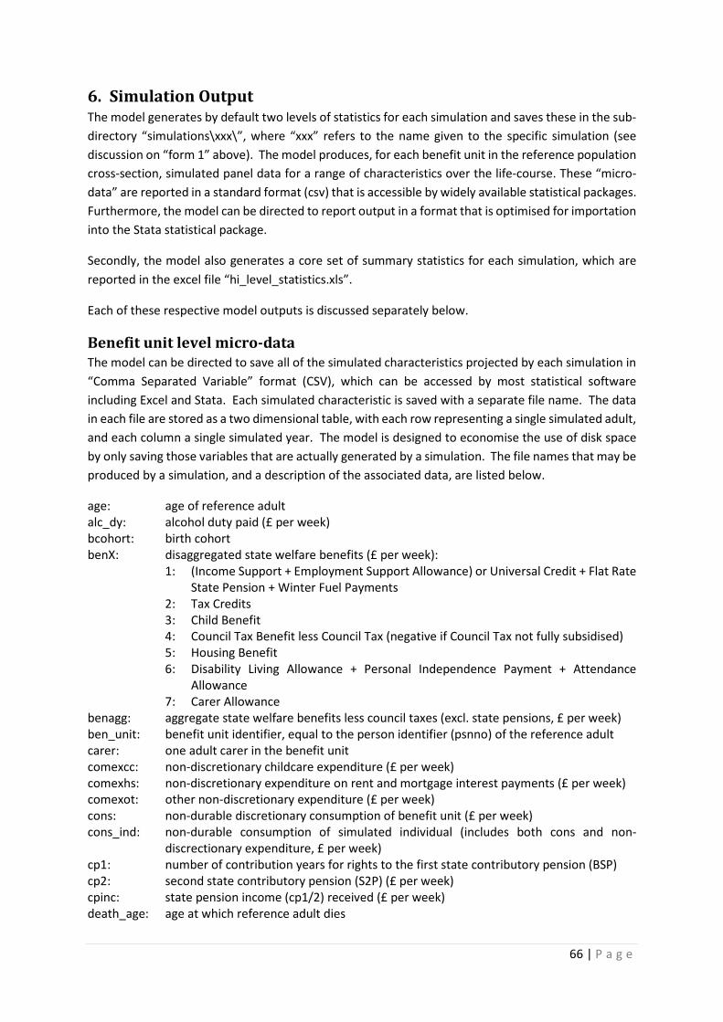
6. Simulation Output The model generates by default two levels of statistics for each simulation and saves these in the sub-directory “simulations\xxx\”, where “xxx” refers to the name given to the specific simulation (see discussion on “form 1” above). The model produces, for each benefit unit in the reference population cross-section, simulated panel data for a range of characteristics over the life-course. These “micro-data” are reported in a standard format (csv) that is accessible by widely available statistical packages. Furthermore, the model can be directed to report output in a format that is optimised for importation into the Stata statistical package.

Secondly, the model also generates a core set of summary statistics for each simulation, which are reported in the excel file “hi_level_statistics.xls”.

Each of these respective model outputs is discussed separately below.

Benefit unit level micro-data The model can be directed to save all of the simulated characteristics projected by each simulation in “Comma Separated Variable” format (CSV), which can be accessed by most statistical software including Excel and Stata. Each simulated characteristic is saved with a separate file name. The data in each file are stored as a two dimensional table, with each row representing a single simulated adult, and each column a single simulated year. The model is designed to economise the use of disk space by only saving those variables that are actually generated by a simulation. The file names that may be produced by a simulation, and a description of the associated data, are listed below.

age: age of reference adult alc_dy: alcohol duty paid (£ per week) bcohort: birth cohort benX: disaggregated state welfare benefits (£ per week):

1: (Income Support + Employment Support Allowance) or Universal Credit + Flat Rate State Pension + Winter Fuel Payments

2: Tax Credits 3: Child Benefit 4: Council Tax Benefit less Council Tax (negative if Council Tax not fully subsidised) 5: Housing Benefit 6: Disability Living Allowance + Personal Independence Payment + Attendance

Allowance 7: Carer Allowance

benagg: aggregate state welfare benefits less council taxes (excl. state pensions, £ per week) ben_unit: benefit unit identifier, equal to the person identifier (psnno) of the reference adult carer: one adult carer in the benefit unit comexcc: non-discretionary childcare expenditure (£ per week) comexhs: non-discretionary expenditure on rent and mortgage interest payments (£ per week) comexot: other non-discretionary expenditure (£ per week) cons: non-durable discretionary consumption of benefit unit (£ per week) cons_ind: non-durable consumption of simulated individual (includes both cons and non-

discrectionary expenditure, £ per week) cp1: number of contribution years for rights to the first state contributory pension (BSP) cp2: second state contributory pension (S2P) (£ per week) cpinc: state pension income (cp1/2) received (£ per week) death_age: age at which reference adult dies

67 | P a g e

donor: psnno of adult used to initialise characteristics (for maturing children and immigrants) dppart: flag = 1 if default is to participate in personal pensions / 0 to not participate education: highest education level achieved during the simulated lifetime (1 = lowest qualification,

n = highest), in order of attainment (right columns come later – interpret with reference to educndage)

educndage: ages at which education level changes emp1/2: employment status of benefit unit reference adult / spouse (0 indicates non-

employment, and n indicates full-employment, where n = the total number of possible labour states, minus 1; intermediate numbers indicate intermediate employment states).

emig_age: age emigrated out of simulated population eqs: equivalence scale ful_dy: fuel duty paid (£ per week) hlthstate: indicator for health / disability states – poorer states take higher values hsgmd: housing mortgage debt (£) hsgmr: housing mortgage interest (£ per week) hsgrret: post-tax realised capital gain on housing wealth (£ per week) hsguret: unrealised capital gain on housing wealth (£ per week) hsggw: gross wealth held in housing (£) humcap: benefit unit human capital (wage potential) (£ per week) ihr_dy: insurance, higher rate duty paid (£ per week) immig_age: age immigrated into model population immig_type: immigrant region of origin (where accommodated) inherit_age: age at which inheritance received inherit_val: value of inheritance (£) isa: wealth held in Individual Savings Accounts (ISAs, £) isa_cont: contributions to ISAs (£ per week) isr_dy: insurance, standard rate duty paid (£ per week) labinc: labour income of benefit unit (£ per week) leis: proportion of time spent in leisure na: number of adults in benefit unit (1=singles 2=couples) net: benefit unit net (disposable) income (£ per week), excluding returns to housing nic: National Insurance Contributions of benefit unit (£ per week) ninvinc: net investment income on generic “other” wealth nk: aggregate number of dependent children nk_allX: number of children, in birth age X nkd_allX: indicator that one child from birth age X is disabled obw: own business wealth (£) parttr1/2: participation tax rates of reference person / spouse peninc: private pension (PP+OP) income received (£ per week) ppc: private pension contributions (£ p.w.) PPcont: aggregate contributions to private pension (including employer contribution) (£ p.w.) PPcr: type of private pension to which benefit unit may contribute (integer = 1,…, n where n

= total number of private pension schemes considered; only reported if more than 1 scheme available).

PPpen: aggregate accrued rights to private pension, defined as an annuity stream (£ p.w.) PPpenb: aggregate accrued rights to private pension, defined as a wealth equivalent (£) prec: age at which pension income first received prett: pre-tax and benefit benefit unit income (£ per week) psnno: unique person identifier region: internal geographic region

68 | P a g e

1= North East; 2=North West; 3=Yorkshire and Humber; 4=East Midlands; 5=West Midlands; 6=East; 7=London; 8=South East; 9=South West; 10=Wales; 11=Scotland; 12=Northern Ireland; ret: whether benefit unit defined as retired for pension purposes ri: proportion of wealth invested in risky assets risky_r: return to risky assets semp: self-employment flag (=1 implies self-employed, if working) student: student status (0 = non-student, 1= type 1 student, 2=type 2 student) taxX: benefit unit tax burden paid in tax band X (£ per week) taxagg: aggregate benefit unit tax burden (£ per week) tbc_dy: tobacco duty paid (£ per week) train_decis: NOT APPLICABLE training: NOT APPLICABLE traintime: NOT APPLICABLE user_taxX: user defined output X from tax routines unempins: NOT APPLICABLE Val: measure of expected lifetime utility vat_rr: reduced rate VAT paid (£ per week) vat_sr: standard rate VAT paid (£ per week) w: liquid wealth of benefit unit (£) w2: aggregate benefit unit net worth (£) wage_offer: flag = 1 if reference adult receives wage offer, 0 if they do not wage_offer2: flag = 1 if spouse receives wage offer, 0 if they do not yrenter: year entered simulation sample – sample ordered from earliest to latest year The following relationship describes the evolution of liquid wealth in most periods:

wt+1 = wt + nett + hsgurett + inheritt – const – comexcct – comexhst + – comexott – isa_contt – sum(indirect taxes)t (1)

The exceptions are when relationship status changes, when a benefit unit first accesses private pension wealth, or when either the upper or lower bound on w is encountered. In the last of these cases, w is constrained to remain within the considered bounds.

prettt = labinct + peninct + hsgrret t – hsgmr t +ninvinc t (2)

nett = prettt + benaggt + cpinct – taxaggt – nict – ppct (3)

The variable net represents the model’s projection for disposable income before housing costs, as used in the DWP’s HBAI publication. Disposable income after housing costs can be evaluated as: net - comexhs.

Default summary statistics

High-level summary statistics - hi_level_statistics.xls The high level statistics that are reported by the model fall into two broad categories, which are each represented by a separate table. Simulated population averages for key benefit unit income, consumption, and balance sheet items are reported in one table, and statistics relating to the macro-economy are reported in the other. The population averages that are reported in the first table are

69 | P a g e

reasonably self-explanatory. The statistics relating to the macro-economy, however, warrant further comment.

Economic analyses of the type for which LINDA has been devised can typically be distinguished in relation to their treatment of factor prices. On the one hand, partial equilibrium analyses assume that factor prices are fixed; this is also commonly referred to as the small open economy assumption. On the other hand, the alternative assumption is that factor prices adjust endogenously to reflect changes in demand and supply. In the case of LINDA, the analyst can choose between these two basic frameworks, as noted in relation to Form Z. Here, directing the model to generate results for the General Equilibrium in a closed economy results in the model adjusting interest rates and wage rates to reflect changes in the supply of capital and labour that are implied by the respective simulation.

The basic idea is that, if saving increases, then this raises the supply of capital in the economy. Increasing the supply of capital in the economy, all else held fixed, should reduce the rate of return paid to capital. This is simulated by LINDA on the assumption that aggregate production, Y, combines aggregate capital, K, and labour, L, in the form of a CES function:

( )( ) εεε /111

/11/11 1 −−− −+= LaaKAY

Assuming that factor markets are perfectly competitive implies that capital and labour are paid their respective marginal products, so that the interest rate, r, and wage rate, w, are given by:

( )( )

( ) ( )( ) εε

εεε

εε

εεεδ

/11/1

/11/11/1

/11/1

/11/11/1

11

1

−−−−

−−−−

−+−=∂∂

=

−+=∂∂

=+

LaaKLaALYw

LaaKAaKKYr

where δ is the rate of depreciation of capital. The aggregate capital stock is set equal to aggregate benefit unit wealth less government debt. Similarly, aggregate labour supply is set equal to the aggregate wage bill, and these two (capital and labour) are combined to give aggregate production as described by the CES function referred to above. Investment is I = (δ + g).K, where g is the assumed growth of the economy. Government consumption, G, is then calculated to equate aggregate income to expenditure:

ICYG −−=

where C is aggregate benefit unit consumption. It should be noted that we do not consider the issue of the government budget balance because we do not cover all of the forms of taxation that are applied in practice (for example, LINDA currently omits taxation of firms).

When directed to generate results for the General Equilibrium in a closed economy, the model iteratively adjusts interest rates, r, and wage rates, w, until these are consistent with the associated aggregates generated for output, capital and labour supply. Note, however, there is no guarantee that the model will converge. The analyst is given a warning if the model has failed to find a solution after searching over 25 alternative parameter combinations, and can choose to continue with the analysis or cancel out in that case.

70 | P a g e

Optional summary statistics The model can be directed to report results from a set a pre-programmed analysis routines. These routines are designed to report data to dedicated Excel files, as described below.

Please note that, at the time of writing, a compiler error has been introduced with new versions of Windows that affects communications with Excel. Wherever this problem has been identified, we have addressed it by outputting the computed statistics in a CSV format. When the associated Excel files (described below) are first opened, they will display zeros wherever saved statistics should be. In this case, please press ALT+F8, and run the “data_update” macro. We have brought this issue to the attention of Intel’s software engineers, and hope that it will be addressed in a more satisfactory manner shortly.

High level analysis of population cross-sections and birth cohorts The model can be directed to report age specific summary statistics for selected population cross-sections and birth cohorts. Where the model generates statistics for a cross-section, then it will save results into a file named “NNN YYYYcs.xls”, where NNN is replaced by the simulation name, and YYYY by the year of the relevant cross-section. Similarly, birth year statistics are saved into a file named “NNN YYYYby.xls”. This analysis routine delivers age and relationship specific moments for labour supply, employment income, disposable income, consumption, private pension participation, and wealth, each in a separate worksheet. Statistics are reported in both tabular, and graphical form.

Poverty statistics A workbook “poverty analysis.xls” is generated by the program and is placed in the sub-directory given by the simulation name. These statistics are specifically designed to consider the trade-off between the bearing of income support programs on the government budget and the incidence of poverty. A series of alternative metrics are used to generate poverty rates:

1. Distributional measures: a. Disposable income before non-discretionary expenditure b. Disposable income after non-discretionary expenditure c. Consumption

i. Non-equivalised and equivalised (using the OECD scale) 2. Population subgroups:

a. Full population b. Children under age 5 c. Single pensioners (over state pension age) d. Couple pensioners (over state pension age)

3. Cross-section specific and over a five year time horizon.

Decile-level summary statistics for population cross-sections and birth cohorts A workbook analysis_dec.xls is generated by the programme and is placed in the sub-directory given by the simulation name. Users are likely to be interested in both the absolute values and the differences from the base, which are each reported in separate worksheets.

The decile groups reported in the spreadsheet are each comprised of one tenth of the weighted sample population that survives to a given period, where lower deciles describe the circumstances of benefit units with lower lifetime income as observed in the prevailing policy counterfactual. Lifetime

71 | P a g e

income is calculated as the present discounted value of the net (disposable) income stream, averaged over the period of survival. Survival probabilities in the model depend only on age and birth year. This means that, when considering evolving characteristics for a given birth cohort, then each benefit units will (approximately) contribute to the same lifetime income decile throughout its life-course.

The difference statistics hold all factors other than the assumed policy parameters constant between the base and counterfactual simulation populations. Hence, each benefit unit is subject to the same random draws in the two sets of simulations, and each “decile” reported in the spreadsheet is comprised of the same sample of benefit units at all points in time. This is crucially important to distinguishing the simulated responses to changes in the policy environment from other modelling considerations. A useful check that this aspect of the model is working as intended is to run a counterfactual simulation that holds all parameters fixed as the same parameters as for the simulation base. Difference statistics calculated between this test simulation and the base simulation should be very close to zero (subject to some rounding errors).

The statistics reported in the spreadsheet are defined in Table 1. As is implicit in the above discussion, the sheet shows arithmetic differences for all variables except the value function. Differences in expected lifetime utility between a given simulation and the associated simulation base are expressed either as compensating variations (£ of liquid wealth equivalents) or percentage differences, as little meaning can be given to absolute differences.

72 | P a g e

Table 1 Data in Analysis_Dec.xls and Differences_Dec.xls Variable Notes and Definitions.

number of benefit units contributing to statistic

Provides a measure of the un-weighted sample size contributing to the reported statistics – this provides an indication of the statistical reliability of the reported statistics (noting that each decile will be comprised of approximately 1/10 of the total population sample, and means based on fewer than 20 observations should be treated as approximate only).

number of adults Describes number of adults in benefit unit

consumption Consumption, including non-discretionary expenditure. (£ per week)

leisure This is the proportion of the leisure available to someone who does not work. Someone who works full-time is defined as having leisure of 0.5. The ratio of the part-time working week to the full-time working week is user-determined in Form 1 as Part-time Ratio (1) for single people and the Lab Ratio variables for couples.

proportion employed Proportion of population with any employment

gross labour income Average income from employment (£ per week)

average contribution to private pension

Average employee and employer contributions to private pensions over decile (£ per week)

propn contributing to private pension

Proportion of decile making any contributions to private pensions

private income private income = (gross labour income) + (investment income on non pension wealth) – (interest on debt) – (private pension contributions) (£ per week)

disposable income disposable income = private income - taxes + benefits (£ per week)

unsecured debt Average value of unsecured debts by population decile (£)

propn of population with unsecured debts

Proportion of decile with negative net liquid wealth (cash on hand)

net non-pension assets Average value of net non-pension assets by population decile (£). Based only on data for benefit units without unsecured debt.

pension wealth Average value of assets held in pensions (£)

total wealth total wealth = (net non-pension assets) – (unsecured debt) + (pension wealth) (£)

value function Remaining life-time welfare. Utility Units. Percentage rather than absolute differences should be considered.

upper threshold for decile

Threshold used to allocate benefit units to deciles as considered in relevant worksheet

73 | P a g e

7. Best Practice Methods of Use This section provides a brief step-by-step guide concerning how the model should be used to explore the effects of policy alternatives. The guide has been written so that it will be applicable to a wide range of alternative subjects of interest, from studies concerned solely with the distributional implications of policy, to those that focus on behavioural responses to policy counterfactuals. Each step of a stylised analytical problem is described under a separate section heading, in approximate chronological order. At the end of each step we provide a practical example of the tasks involved with reference to the policy counterfactual in which 10 percentage points are added to the highest rate of income tax in the base policy specification assumed for the model.

TIP: it is incredibly important that you allow ample time to conduct your analysis.

Step 1: specify policy parameters There are two alternative ways to alter the policy environment in the model. The first is to alter the parameters of the existing model structure. New users of the model are encouraged to select policy parameters using the Excel front-end that is supplied with the file “job file.xls”, as described in Section 3. Advanced users may find it easier to alter model parameters directly through the cells on the “input” sheet of “job file.xls”. The second alternative is to alter the tax code directly; see Section 8 for details.

Having adjusted the model parameters, it is often advisable to check that the revised structure conforms to that which is desired. A number of tools are provided with the model to facilitate such checks.

Checking differences with base simulation The “check” tab in “job file.xls” allows you to identify which parameters in the “input” sheet are different to those of the base simulation (stored in the “inputA” sheet). You can run this check after working through the front-end forms in “job file.xls” in one of two ways. If you press the “LAUNCH MODEL” button on Form Z, then you can look at the “check” tab after the fortran program has started. Alternatively, you can choose the “EXIT” button on Form Z, saving “job file.xls”, and then look at the “check” tab. In this second case, after you have confirmed that you are happy with the differences described between the prevailing model parameters (sheet “input”) and the model base (sheet “inputA”), you can launch the Fortran code manually by double-clicking on the program SIDD.exe.

Validating the tax function As noted in Section 3 (Form D4), there are two routines that are provided with the model that produce trial statistics for the simulated tax function. The terms of both test routines are defined by Excel files stored in the “MODEL\analysis_files\” subdirectory. “tax_test1.xls” allows you to generate test statistics for a range of alternative pre-tax incomes, for a given benefit unit type. “tax_test2.xls” is similar to “tax_test1.xls”, but allows you to vary both pre-tax income and benefit unit demographic characteristics.

These test routines can be run at any time after you have started running a given simulation.

1) Open the relevant excel file (“tax_test1.xls” or “tax_test2.xls”). 2) Define the alternative test cases that you would like to consider

74 | P a g e

3) Save the excel file. 4) Open “job file.xls” 5) Run the SIDD macro 6) Enter the relevant simulation name in the text box adjacent to the button “ANALYSE TAX

FUNCTION” 7) Press the “ANALYSE TAX FUNCTION” button. 8) Select the relevant analysis routine using the radial button. 9) Press the “ENTER and RUN” button.

A new simulation window will open, and will indicate when the analysis routine is complete. You can then re-open the relevant excel file (“tax_test1.xls” or “tax_test2.xls”) to check the results obtained.

Example We are interested in considering the effects of increasing the higher rate of income tax by 10 percentage points. Our example assumes that a model “base simulation” has already been run, as described in Section 2 of this manual. We alter the model parameters through the Excel front-end, as indicated in the following sequence of User Forms.

1. PRESS THE “SET UP NEW SIMULATION” BUTTON

75 | P a g e

2. Enter a reference for the “Simulation Name”, and then press the “ENTER” button.

76 | P a g e

3. We are running an analysis of a policy counterfactual. It is likely to take some time for you to work out your preferred approach for this type of task. In our experience, we have found decile level statistics of differences with the base population for a younger birth cohorts to be particularly useful in gaining a high-level picture of how a given policy alternative influences individual circumstances. Developing this type of narrative should be your first objective, as it will help you to interpret most statistics of interest. The model is directed to undertake this analysis by altering the front-end as indicated above.

WE SKIP FORM 3, WHICH DOES NOT NEED TO BE ALTERED

77 | P a g e

4. Form Aa1 lists the policy parameters that we are interested in altering. Here, we add 10% to each of the terms highlighted above. As these are the only changes to the policy environment that we are interested in, we can then press the “ENTER and RUN” button as indicated.

78 | P a g e

5. It will usually be sensible to assume the “BASE Specification”, which has been carefully selected to balance accuracy against computation time. Here we then press the “EXIT” button, as we would like to check over the parameter changes that have been implemented by the model front-end.

79 | P a g e

6. Go to the “check sheet” of “Job File.xls”. The total number of parameter differences with the model’s base simulation are reported in cell A1 of this sheet (19). Looking across row 1 of the sheet will indicate which columns include altered parameters.

80 | P a g e

7. Scrolling across row 1, we see that the first column that has been altered by the front-end is AJ. Cell AJ1 indicates that 4 parameters in this column have changed, and searching down the column indicate that values of rows 14, 106, 107, and 108 have all altered. Checking the base parameters (in sheet inputA) against the model parameters described for the current simulation (sheet input) indicates that the front-end has increased the higher rates of tax as it was directed to do (step 4 above).

CONTINUING TO CHECK ACROSS THE “check” WORKSHEET INDICATES THAT THE ONLY OTHER MODEL PARAMETERS ALTERED FROM THOSE IN THE BASE SPECIFICATION CONCERN “ANALYSIS PARAMS”, WHICH INFLUENCE THE NATURE OF THE SIMULATION STATISTICS THAT WILL BE GENERATED INTERNALLY BY THE MODEL.

81 | P a g e

Step 2: run model and generate output As noted in Section 4, two types of output can be generated by the model. The model will solve simulated panel data for each benefit unit, in the form of *.csv files (that can be opened by most statistical packages). In this case, each variable is saved in a separate file, each row represents a different benefit unit, and each column a different time period.

The model will generate a series of summary statistics for each simulation by default, which are reported in Excel files. The model can also be directed to generate a range of additional summary statistics; see Section 4 and “Form 2” in Section 3 for further details.

Example 8. Having verified the model parameters for the new simulation correspond to those that we

are interested in, we can launch the model program. • Save the file “Job File.xls” • Double click on the executable file “SIDD.exe”, to launch the model program, and

wait for the model window to indicate that it is finished.

82 | P a g e

Step 3: think about likely incentive effects An important feature of the model is that savings and labour supply decisions are endogenous. This means that these decisions react to the incentives that are embodied by the assumed policy environment. Explaining the results that are reported by the model consequently depends in part on understanding the drivers underlying the simulated behaviour. It is useful to think about what behaviour you expect to see before the model completes its analysis, as this will help you to identify where to begin looking once the simulated results are in. It is easiest to think about incentives relative to the base simulation, as the model can be asked to generate comparisons with the base simulation by default.

Example 9. We have raised the marginal tax rate of all higher rate payers by 10 percentage points. This

can be expected to have a large number of effects on the simulated population. Some of the most important are listed here in bullet point form:

• Higher tax rates imply two key effects: i. Affected benefit units will have lower lifetime income in the absence of any

behavioural responses – this consideration will motivate responses that are sometimes referred to as a “wealth” or “income” effects.

ii. Affected benefit units will be subject to higher effective marginal tax rates on labour income, and on investment income that is not tax-shielded – this consideration will motivate responses that are sometimes referred to as “price” or “substitution” effects.

• Likely wealth effects: i. Lower consumption

ii. Increased employment iii. Lower saving

• Likely substitution effects: i. Higher consumption, as effective post-tax returns to saving decrease

ii. Lower employment, as the marginal returns to labour supply have fallen iii. Lower saving in assets that are subject to taxes iv. Increased saving in assets that are tax shielded.

Step 4: analyse model output This stage of the analysis involves comparing the model output against the expectations that you formed in Stage 3 (described above). It is not uncommon to find that behaviour deviates from what you had initially expected, as the incentives embodied by policy can often be quite difficult to infer.

High level analysis The model produces a large number of high-level summary statistics by default in the file DA1.xls. It can also be directed to report a series of age specific statistics for population cross-sections and individual birth cohorts (see Section 3). Through repeated use, you are likely to settle upon some subset of these results as an appropriate place to start your analysis.

Detailed statistical analysis The model can be used to generate decile level statistics, and to produce associated comparisons with the base population. These statistics will often be sufficient to identify the key margins of

83 | P a g e

behavioural variation simulated under a given policy environment, and allow you to formulate a “story” underlying the results obtained.

What to do when results do not conform to expectations If the above statistics do not enable you to devise a compelling account of the results generated by the model, then it is often useful to focus upon the micro-data generated by for individual benefit units. Suppose, for example, that you cannot understand why labour supply falls under the policy environment of interest, relative to the base simulation. In this case, you could look for units that are simulated to reduce their labour supply substantively under the new policy environment. Bearing in mind that the model is designed so that the only differences between alternative simulations are due to the considered policy environments, this approach will hopefully provide clues as to the incentives that underlie the unanticipated behavioural responses. As a last resort, staff at the NIESR will attempt to provide technical support (subject to availability).

Example As noted under “Step 1” above, we often find it useful when interpreting responses to policy changes to begin with the difference statistics that can be reported for population deciles by the model (implemented by point 3 above). These statistics are reported in the excel file “analysis_dec.xls” that should be saved in the \simulations\NAME subdirectory, where “NAME” here refers to the name you chose to give the simulation run (see point 2 above). The difference statistics with the base simulation are reported in the “differences with base” worksheet. Details of the statistics reported in this file are described in Section 5.

It is noted in Section 5 that the difference statistics generated by the model are designed so that the only variation between a policy counterfactual and the simulation base relates to the simulated policy conditions. If you have worked through the above example, then you should find that there are zeros for all statistics relating to the number of adults, and for all statistics reported to age 35. These results are obtained because (i) the same benefit units contribute to each decile group in the counterfactual and base simulations; (ii) the same random draws are used to project circumstances through time (implying the same number of adults for each benefit unit in each simulation); and (iii) our counterfactual simulation projects forward through time from 2006 and we are focussing here on the birth cohort born in 1970, so that the counterfactual simulation only affects the considered birth cohort from age 36.

In columns to the left of the decile level statistics reported in the “differences with base” worksheet are age specific population averages for each of the variables reported in the spreadsheet. A selection of these statistics is reported in Figure 7.1 to Figure 7.4.

Figure 7.1 indicates that the policy counterfactual tends to result in higher rates of employment, relative to the base simulation. The model consequently suggests that benefit units will try to off-set some of the higher tax burden implied by a 10 percentage point increase in the higher tax rate through increased labour supply. Hence, the “wealth effects” referred to under point 9 above dominate the “substitution effects” for labour supply.

Figure 7.2 indicates that average private incomes increase under the policy counterfactual, consistent with the rise in employment referred to above. But the rise in private income is insufficient to off-set the increased tax burden fully, so that disposable income in the policy

84 | P a g e

counterfactual is lower than in the base simulation. The lower lifetime income that is implied by a depressed disposable income stream leads consumption to shift down in all periods following the considered change in policy.

Figure 7.3 displays the influence of the policy counterfactual on savings. Consistent with the depressed disposable income stream under the policy counterfactual, “total net wealth” is projected to fall on average as a result of the policy change. It is notable, however, that investment allocations also vary under the two policy contexts, with simulated benefit units saving more through pensions (that enjoy tax shielding) in context of increased marginal tax rates.

Figure 7.4 provides an indication of the dispersion of the population average effects discussed above. This figure indicates that high lifetime income people are disproportionately affected by the considered policy change, which is unsurprising given the nature of the policy change.

Note, however, that it is not uncommon to observe behavioural variation distributed quite widely by the model, even where a considered policy counterfactual is tightly targeted. This is because temporal variation of individual specific circumstances can see individual benefit units move into and out of contexts where they are affected by a targeted policy change. Furthermore, the uncertainty that characterises temporal variation of individual specific characteristics can motivate behavioural variation even amongst benefit units who are never directly affected by a considered policy reform. In the current example, it is therefore possible to identify benefit units who are never actually subject to the higher rate of tax (and are therefore not directly affected by the policy counterfactual), but who nevertheless alter their behaviour due to the possibility that they might be subject to the higher marginal rate of tax at some point in the simulated future.

Figure 7.1: Average effects of increasing the higher rate of tax from 40 to 50 percentage points in 2006 on the proportion of adults employed of population birth cohort born in 1970

-0.002

0

0.002

0.004

0.006

0.008

0.01

15 25 35 45 55 65 75 85 95

age

proportion of adults employed

85 | P a g e

Figure 7.2: Average effects of increasing the higher rate of tax from 40 to 50 percentage points in 2006 on financial flows of population birth cohort born in 1970

Figure 7.3: Average effects of increasing the higher rate of tax from 40 to 50 percentage points in 2006 on financial stocks of population birth cohort born in 1970

-15

-10

-5

0

5

10

15

15 25 35 45 55 65 75 85 95

age

consumption (£ per week) private income (£ per week)

disposable income (£ per week)

-4000

-3000

-2000

-1000

0

1000

2000

3000

15 25 35 45 55 65 75 85 95

age

net (non-pension) assets (£) pension wealth (£)

total wealth (£ net of debt)

86 | P a g e

Figure 7.4: Effects on consumption of increasing the higher rate of tax from 40 to 50 percentage points in 2006 on the birth cohort born in 1970, by lifetime income decile

Step 5: package output Having identified a behavioural “story” underlying simulated results, the packaging exercise is usually fairly straight-forward. As this exercise will vary, depending upon the subject of concern, we do not discuss it further here.

-30

-25

-20

-15

-10

-5

0

5

15 35 55 75 95

cons

umpt

ion

effe

ct (£

per

wee

k)

age

1

4

6

8

10

decile

87 | P a g e

8. Adjusting the Program Code The model is programmed in Intel Visual Fortran, and users have access to the routines that calculate taxes and benefits. The tax routines can be edited through Microsoft Visual Studio at the time of writing (the steps involved in setting-up this environment for use are provided in Section 2). In this section we describe some programming basics, before running through a practical example for simulated tax and benefits policy.

Programming basics

Basic Code Structure • The Fortran code that is provided with the model is organised into four broad structures,

which can usefully be thought of as containers. • The largest container is the “solution”, which is a set of files that comprise the basic building

blocks that Fortran uses to generate program files o The “TAXES solution” can be opened by double-clicking on the file “TAXES.sln” in the

“FORTRAN\TAXES\” subdirectory. • The second largest container is the “source file”, into which code is written.

o You can browse through the source files of a solution via the “Source Files” folder of the “Solution Explorer” (which can be seen by selecting “Solution Explorer” from the “View” menu of Visual Studio)

o To add a new source file to a solution: right click on the Source Files folder

• select “add”, “new item” • select “Fortran Free-form File (.f90)” • make up a name for the file toward the bottom • and press the “Add” button

• Each source file can contain one, or a number, of MODULEs. o A MODULE is predominantly a container to organise a number of SUBROUTINEs.

e.g. MODULE AA might contain SUBROUTINEs AA1 and AA2; and MODULE BB might contain SUBROUTINEs BB1 and BB2

a slight complication arises in relation to “global variables”, which is returned to below.

• Most MODULEs are organised as follows: o MODULE AA

This line denotes the start of the MODULE with the name AA o IMPLICIT NONE

This line is necessary to avoid easy programming errors – do a google search on it for further detail

o CONTAINS This line notes that the SUBROUTINES that follow are contained within the

MODULE o **** SUBROUTINEs then appear here **** o END MODULE AA

This line denotes the end of the module • All of the program computations are undertaken by code that is organised within a series of

SUBROUTINEs. o e.g. SUBROUTINE AA1(x, y) takes a series of inputs x, performs a number of

calculations, and then returns a series of outputs y. We would execute this subroutine by entering the following code:

call AA1(x,y)

88 | P a g e

• To use (call) SUBROUTINE XX from within SUBROUTINE YY, either: o the two SUBROUTINEs must be organised within the same MODULE, or

SUBROUTINE YY must be given access to the MODULE containing SUBROUTINE XX e.g. in the above example SUBROUTINE AA1 could call AA2 by default, but

would need to be given access to MODULE BB to call BB1 (or BB2) • Each SUBROUTINE must be organised as follows (based on the above example):

o SUBROUTINE AA1(x, y) This line denotes the start of the subroutine, and the variables that are used

as inputs and outputs – if the subroutine takes in no explicit inputs, and produces no explicit outputs, then we write “SUBROUTINE AA1()”

o USE BB This line gives SUBROUTINE AA1 access to the SUBROUTINEs contained in

MODULE BB This line is only required if you want to access SUBROUTINES (or global

variables) stored in MODULE BB o IMPLICIT NONE

This line is necessary to avoid easy programming errors – do a google search on it for further detail

o real (8) :: x, y This line of code refers to the “type definitions”, and usually covers a

number of lines. A “type definition” tells fortran the explicit nature of the data that each

variable contains. The variables that you will most commonly require will be limited to real(8)

(a number with a decimal point) and integer(4) (a whole number without any decimals) types.

• A variable cc is assigned a real type by; real(8) :: cc • A variable cc is assigned an integer type by; integer(4) :: cc • If cc is a matrix of real numbers with dimension (5,4) (5 rows and 4

columns), then it is assigned by; real(8) :: cc(5,4) You must assign types to all of the variables that are included as inputs and

outputs to a given subroutine (e.g. x and y in the example here) You must also assign types to all of the variables that you use within the

subroutine, and which are discarded after the subroutine is complete • Variables discarded after a subroutine is complete are commonly

referred to as “local variables”. o **** You then add in programming code to undertake your desired calculations

here **** o END SUBROUTINE AA1

This line denotes the end of your subroutine

The above covers just about everything you will need in relation to program structure. There is, however, one final complication. Fortran requires each variable that is used in any subroutine to be assigned a type (real / integer above). In most cases, the variables that you use will either be explicit inputs / outputs of a subroutine, or will be “local variables” that you don’t mind discarding after your desired computations within the subroutine are complete. Nevertheless, there are a number of variables that you might want to make common to a range of subroutines, without needing to repeatedly pass these variables as explicit inputs to each subroutine. Examples in relation to tax and benefits calculations include the number of adults and children in a benefit unit, the employment

89 | P a g e

status of adult benefit unit members, measures of gross income, and so on. This is achieved in the code using “global variables”.

• You will find in the set of source files included with the TAXES program, one called “2_global.F90”.

• If you open this file, then you will see that it includes a module named “global_tax”. o The MODULE global_tax includes a series of variable type definitions, and no

subroutines. o The variables defined within this module are referred to as “global variables”. This is

because it is possible to share them between alternative subroutines without the need for explicit declarations.

• The global variables defined in MODULE global_tax are assigned values within the SUBROUTINE initialise_taxinputs (see Figure 1), found in the source file “1_TaxTools.f90”

o Note that SUBROUTINE initialise_taxinputs is given access to the global variables by the “USE global_tax” declaration at line 23

• Any SUBROUTINE that subsequently requires access to the global variables needs only to include the declaration “USE global_tax” in its second line of code (as outlined above for SUBROUTINE structure)

Common programming steps It is beyond the scope of this manual to provide detailed advice concerning programming of new analysis procedures, which is best understood by obtaining hands-on experience. Here we provide a brief over-view of the steps involved in editing Fortran code, and some advice concerning use of the debugging environment.

The following steps are usually involved when editing the Fortran code:

1) Open a “program solution” (see the section on “Basic Code Structure” for a description of a “solution”).

2) Edit the program text 3) Save the revised text 4) “Re-build” the solution in a “debug configuration”

a. This essentially tells Fortran to use the new building blocks to create new program files

b. The debug configuration is designed to enable you to check that your revised program works as intended

5) Run some test analyses to make sure that the revised code works as intended 6) “Re-build” the solution in a “release configuration”

a. The release configuration is designed to omit the checks implemented in the debug configuration, and typically works much faster as a result

7) Run your desired analyses

The following will walk you through how to set-up the debugger, essentially addressing steps (1) and (4) listed above, with reference to the TAX routines provided with the model.

90 | P a g e

Opening a “Solution”

1) Double click on the file “TAXES.sln” in the subdirectory “FORTRAN\taxes\” a. This should open up the Visual Studio (VS) programming environment b. If you followed the steps set out in Section 2, this solution is now ready for editing

(please ensure that this is the case). 2) In the “solution explorer” window, expand the “source files” folder

a. If the “solution explorer” window is not open, then you can open it by selecting the “View” menu at the top of VS, and then “Solution Explorer”

b. The following source files should be listed under the “source files” folder: i. 0_app_taxes.f90

ii. 1_TaxTools.f90 iii. 2_gobal.f90 iv. AUS_1.f90 v. IE_1.f90

vi. IT_1.f90 vii. UK_1.f90

viii. UK_2.f90 ix. UK_3.f90 x. UK_4.f90

3) Double click on the file “UK_3.f90” a. This should open a text file in the main window of Visual Studio

4) Press CNTRL+HOME a. This should move the cursor to the top of the text file (if it wasn’t already).

5) Toward the top of the text window, you should see a grey bar that is split into two parts. Click on the left part (which should have “UK_params3” listed in it)

6) Select “UK_tax3” (this text file has two “modules” in it) 7) Click on the right part of the grey bar, which lists all of the subroutines in the current module 8) Select “UK_3” from the drop down menu

a. This will move the cursor to the beginning of the SUBROUTINE UK3

Re-build the Solution in a “Debug Configuration”

1. Select the appropriate compile settings a. In the “solution explorer”, highlight the purple icon “TAXES” b. Under the view menu of VS, select “Property Pages” c. From the “Property Pages” window, press the “Configuration Manager” button d. Under “Active solution configuration:”, select “debug” e. Under “Active solution platform:”, selection “x64” f. Press the “Close” button g. Press the “OK” button

• You can also do the above more easily by selecting the “Active solution configuration”, and “Active solution platform” from the drop-down windows of VS, which may be visible as toolbars in the VS environment.

2. Build the solution a. From the “Build” menu of VS, select “Clean Solution” b. From the “Build” menu of VS, select “Build Solution”

• You should see the following output:

91 | P a g e

1>------ Rebuild All started: Project: TAXES, Configuration: debug x64 ------ 1>Deleting intermediate files and output files for project 'TAXES', configuration 'debug|x64'. 1>Compiling with Intel(R) Visual Fortran Compiler XE 15.0.0.108 [Intel(R) 64]... 1>2_global.F90 1>AUS_1.f90 ... 1>IE_1.F90 1>0_app_taxes.f90 1>Compiling manifest to resources... 1>Microsoft (R) Windows (R) Resource Compiler Version 6.3.9600.17200 1>Copyright (C) Microsoft Corporation. All rights reserved. 1>Linking... 1>Creating library C:\MyFiles\MODEL_LAB\MODEL\TAXES.lib and object C:\MyFiles\MODEL_LAB\MODEL\TAXES.exp 1>Embedding manifest... 1> 1>Build log written to "file://C:\MyFiles\MODEL_LAB\FORTRAN\TAXES\x64\debug\BuildLog.htm" 1>TAXES - 0 error(s), 0 warning(s) ========== Rebuild All: 1 succeeded, 0 failed, 0 skipped ==========

c. Check that the files have built to the correct location • Look in the “\model\” subdirectory, and check that new files named

“TAXES” have been generated by the compiler We now turn to the steps involved in programming a new tax routine.

92 | P a g e

Programming a new Tax and Benefits Regime Taxes and benefits in the model can be altered, either by adjusting parameters for pre-programmed schemes (e.g. see Section 3), or by programming new transfer schemes from scratch. This section provides some guidance concerning the second of these two options. We begin by presenting a schematic for the organisation of the tax, and then provide a step-by-step guide to introducing new code into the model. We then finish up the section by describing how to alter the code so that it will generate a set of user defined outputs by default.

Organisation of the Tax and Benefits Code A stylised schematic of how the tax and benefit calculations are organised is provided in Figure 8.1. Arrows and numbers indicate approximate order of access, and associated inter-dependencies.

Figure 8.1: Stylised Schematic of the Calculation of Taxes and Benefits in LINDA

tax_vars(inputs, outputs)

initialise_taxinputs unpacks the variables transferred from LINDA in the vector “taxinput” into individual variables that are useful for analysis

UK_3(inputs, outputs) calculates all outputs for the UK

LINDA

global_tax global variables

UK_params3 global variables (UK)

initialise_taxpars unpacks the variables transferred from LINDA in the matrix “tax_par” into individual variables that are useful for analysis

CalcTax calculates income tax

IncomeSupport calculates means-tested benefits

TaxCredits calculates tax credits

HousingBenefits calculates Housing and Council Tax benefits

1 2

4 5 6

8

3

7 9

10

11

12

return to LINDA

global variable access

UniversalCredit calculates Universal Credit

13

93 | P a g e

Introducing user-defined tax schemes An important feature of the LINDA model is that users can implement new tax and benefit schemes that extend beyond simple parameter adjustments of existing schemes. Suppose, for example, that you wanted to radically alter income support payable to working aged people from the scheme in place in 2010. The following provides a step-by-step guide to introducing a new user defined scheme.

1) Start by defining a test case a. Open file “tax_test1.xls” in the subdirectory MODEL\ANALYSIS_FILES b. Adjust the individual definition to reflect the circumstances of someone affected by

the reform of interest. In our example, set: i. age (cell B1) to 25

ii. year to 2010 iii. number of adults to 2 iv. number of children to 1 v. other values to those of potential interest

c. Save the file d. Close “tax_test1.xls” e. Open “job file.xls” f. selected press ALT+F8 g. Run the SIDD macro h. Press the “NEW SIMULATION FOR THE UK” button i. Under “Simulation Name” type “test” j. Select the “2010 tax benefit model tables” option k. Under the “tax function reference year” type 2010 l. Press ENTER m. In FORM 2, press the “ANALYSE TAXES” button n. In FORM D4, select “Single individual type” o. Press the “ENTER and RUN” button

Step 1 will run a test simulation, and report the output to tax_test1.xls – save a copy of this file under the name temp.xls for reference at a later stage

2) Set the user-defined transfer system to replicate the pre-programmed transfer system for 2010

a. Add the user defined scheme to the Excel “job file” i. Open “job file.xls”

ii. Open the “tax params” worksheet iii. Copy columns 9:14, and paste these into columns 2:7 iv. Save the excel file v. With “job file.xls” selected press ALT+F8

vi. Run the SIDD macro vii. Press the “NEW SIMULATION FOR THE UK” button

viii. In FORM 1: 1. Under “Simulation Name” type “test” 2. Select the “user defined tax structure” option

94 | P a g e

3. Under the “tax function reference year” type 2010 4. Under the “reference number for user tax structure” type “3” 5. Press ENTER

ix. In FORM 2: 1. Press the “ANALYSE TAXES” button

x. In FORM D4: 1. Select “Single individual type” 2. Press the “ENTER and EXIT” button

Here we have altered “job file.xls” so that it will direct LINDA to run a simulation based on a user defined tax structure. The user defined tax structure is denoted by the reference number 3 (step 2.a.viii.4 above). We have also set up “job file.xls” to run a test of the assumed tax structure, which is important to ensuring that the revised model specification reflects that desired by the analyst. We return to this feature below.

b. Add the user defined tax structure to TAXES.sln i. Double click on the TAXES.sln file

ii. Open file “0_app_taxes.f90”, by double-clicking on the file in the Solution Explorer

iii. Copy lines 113 to 116:

elseif ( tax_par4(15).lt.2.5 ) then ! UK 2006 call UK_2(age, year, n_taxp4, tax_par4, ndim_tax, tax_par, yy1, Rpstt, …

iv. Paste these lines at 117 v. At line 117, replace 2.5 with 3.5

vi. At line 118, replace “UK 2006” with “User defined 2010” vii. At line 120, replace UK_2 with UK_3

This adds in a reference to the User Defined tax routine UK_3 into the main TAXES program, using the reference value 3 defined in step 2.a.viii.4 above.

viii. In the Solution Explorer window, right-click on the “Source Files” folder, and select “Add”, and then “New Item”

ix. Select “Fortran Free-form File” x. Under “Name”, enter “UK_3.f90”

xi. From the Solution Explorer window, double click on “UK_1.f90” xii. Press CNTRL+A (to select all)

xiii. Press CNTRL+C (to copy) xiv. From the Solution Explorer window, double click on “UK_3.f90” xv. Press CNTRL+V (to paste)

xvi. Press CNTRL+H (to do a search and replace) xvii. Search for the module name “UK_params1” and replace with “UK_params3”

1. Ensure that the search and replace is limited to the “current document” – UK_3.f90

xviii. Search for the module name “UK_tax1” and replace with “UK_tax3”

95 | P a g e

1. Ensure that the search and replace is limited to the “current document” – UK_3.f90

xix. Search for the subroutine name “UK_1” and replace with “UK_3” 1. Ensure that the search and replace is limited to the “current

document” – UK_3.f90

This sets up the new User Defined code, copying over from the code that is provided with the model for 2010.

xx. From the Solution Explorer window, double click on “0_app_taxes.f90” xxi. At line 58, add “USE UK_tax3”

This permits the subroutine UK_3 to be called from the code we added at step 2.b.vii above.

xxii. From the “File” menu, select “Save All” c. Rebuild TAXES in debug configuration

i. In the “solution explorer”, highlight the purple icon “TAXES” ii. Under the view menu of VS, select “Property Pages”

iii. From the “Property Pages” window, press the “Configuration Manager” button

iv. Under “Active solution configuration:”, select “debug” v. Under “Active solution platform:”, selection “x64”

vi. Press the “Close” button vii. Press the “OK” button

1. You can do the above more easily by selecting the “Active solution configuration”, and “Active solution platform” from the drop-down windows of VS, which may be visible as toolbars in the VS environment.

viii. From the “Build” menu of VS, select “Clean Solution” ix. From the “Build” menu of VS, select “Build Solution”

1. You should see the following output: 1>------ Build started: Project: TAXES, Configuration: debug x64 ------ 1>Compiling with Intel(R) Visual Fortran Compiler XE 15.0.0.108 [Intel(R) 64]... 1>IT_1.f90 1>0_app_taxes.f90 1>Compiling manifest to resources... 1>Microsoft (R) Windows (R) Resource Compiler Version 6.3.9600.17200 1>Copyright (C) Microsoft Corporation. All rights reserved. 1>Linking... 1>Creating library C:\MyFiles\MODEL_LAB\MODEL\TAXES.lib and object C:\MyFiles\MODEL_LAB\MODEL\TAXES.exp 1>Embedding manifest... 1> 1>Build log written to "file://C:\MyFiles\MODEL_LAB\FORTRAN\TAXES\x64\debug\BuildLog.htm" 1>TAXES - 0 error(s), 0 warning(s) ========== Build: 1 succeeded, 0 failed, 0 up-to-date, 0 skipped ==========

x. Look in the MODEL subdirectory, and check that new files, all with the name

TAXES.*** have been generated by the compiler

Step 2 will have added new code into the TAXES routines, and set the model up to call this code.

3) Run a first test case a. In the MODEL subdirectory, double-click on SIDD.exe

96 | P a g e

Steps 1 and 2 have been set up to allow you to check that the new code successfully replicates the 2010 code. Open up the temp.xls file created at the end of step 1, and compare this to the tax_test1.xls file generated following step 3.a – the data in both files should be identical, with the exception that the tax_test1.xls file should be more recent.

b. Ensure that the new code is being used i. In VS, select open file 0_app_taxes.f90

ii. Clear all break-points, by selecting the “Debug” menu from VS, and select “Delete all breakpoints”

iii. Go to line 81 iv. Press F9 – a red dot should appear in the margin as depicted here

As the comment indicates, this piece of code is designed to ensure that the breakpoint will only be encountered if the model is running a test simulation.

v. Press F5 to launch the debugger vi. A yellow arrow should eventually appear at the red dot, indicating that the

model has run to that point. vii. Press F10 to step through the code, one line at a time and check that it does,

in fact, calculate taxes via the UK_3 subroutine that we introduced in step 2 4) Alter UK_3.f90 code

a. In this stage, the tax and benefits code that we copied over from UK_1.f90 to UK_3.f90 can be altered to reflect the schemes of interest.

b. Our experience suggests that this process will involve the following stages: i. Implement new code

ii. Attempt to compile code in debug configuration as described in step 2c above

1. Correct any bugs identified by the compiler iii. Run a test simulation with all break points deleted (see step 3.b.ii above)

1. Correct any bugs identified by the debugger iv. Check implied disposable income schedules, as reported in tax_test1.xls,

trialling alternative population combinations of interest

97 | P a g e

1. Where oddities are evident in the profiles, use the debugger to walk through the associated code to determine where remaining errors lie.

v. Finalise code, and compile in “release configuration”

Adjusting number of tax outputs It is possible to alter the tax code of the model, so that it will generate additional summary statistics to those that are produced by default. This involves the following steps:

1) Define the number of additional statistics in the model parameters. a. Add the number of additional tax statistics that you would like to generate with the

model to the number currently defined in cell AO14 of sheets “input” and “inputA” in “job file.xls”.

i. E.g. if the pre-existing value in cell AO14 is 17, and you would like to add an additional three outputs, then alter this cell to 20.

ii. This step can also be conducted through FORM 1 of the Excel front-end b. Save “job file.xls”.

2) Alter the Fortran code in the solution “TAXES.sln” to generate the statistics of interest a. Note that these statistics need to be included as output variables in the subroutines

that calculate taxes and benefits. e.g. you might alter the subroutine:

call UK_1(age, year, n_taxp4, tax_par4, ndim_tax, tax_par, yy1, cc_costs, hlth_costs, hs_costs, benefit_s, tax_s(1:8))

so that it includes an additional output xx, by including xx at the end of the variable list as in:

call UK_1(age, year, n_taxp4, tax_par4, ndim_tax, tax_par, yy1, cc_costs, hlth_costs, hs_costs, benefit_s, tax_s(1:8), xx)

3) Alter the output vector to return the statistics to the model. a. The additional statistics need to be sent to the subroutine pack_taxoutputs, and

then added to the end of the output vector as directed in that subroutine. e.g. in the above example, we would alter the code as indicated here:

call pack_taxoutputs(taxoutput, n_taxoutput, yy, cc_costs, hlth_costs, hs_costs, benefit_s, tax_s, xx)

and then include xx in taxoutput, just after the line: ! user output add to the bottom here, altering the check imposed by the if statement as necessary

b. As the above comment suggests, it is also necessary to alter the check statement imposed by the if statement at the top of the pack_taxoutputs subroutine to recognise the additional output:

if ( n_taxoutput.lt.20 ) then elseif ( n_taxoutput.gt.20 ) then end if

4) The model will then include the associated statistics in the panel data generated for each simulated population, under the name user_toX, where X = 1, 2, 3, etc, for the first second and third output that has been added to the list of statistics reported by the tax function.

98 | P a g e

TIP: The analysis routines concerned with budgetary aggregates that are included with the model reference BenAgg and TaxAgg variables. If you would like the new scheme that you have programmed to feed into the budgetary statistics generated by these analysis routines, then it is necessary to include the value of any benefit as augmenting an element of the vector benefit_s (in the case of benefits) or tax_s (in the case of taxes).

99 | P a g e

Appendix A: End User License The computational engine upon which LINDA is based is referred to as the Simulator of Individual Dynamic Decisions, SIDD. LINDA is essentially a parameterisation and the policy environment that NIESR has implemented to permit SIDD to consider implications for the United Kingdom. The user license is for use of the SIDD engine. Model parameters assumed by LINDA are either high-level summary statistics that NIESR has calculated, and which are a matter of public record, or micro-data (i.e. the Wealth and Assets Survey) that must be accessed via third-party agreements not covered here.

PLEASE READ CAREFULLY BEFORE INSTALLING Licence Agreement This license agreement ("Licence") is a legal agreement between you (Licensee, or you) and the National Institute of Economic and Social Research, whose address is at 2 Dean Trench Street, Smith Square, London, SW1P 3HE, UK (Licensor, us or we) for the Simulator of Individual Dynamic Decisions Model software ("SIDD"). SIDD is a microsimulation model of tax and benefit systems, including the documentation (printed and electronic). For the avoidance of doubt, SIDD and this agreement does not include source input micro-data from surveys and administrative data sources. We licence use of SIDD to you on the terms of this Licence Agreement. We do not sell the SIDD or accompanying documentation to you. We remain the owners of SIDD at all times. 1. Licence 1.1. In consideration of the mutual promises contained herein the Licensor hereby grants a non-exclusive, non-transferable, non-sublicensable, royalty-free, licence to the Licensee to use SIDD. 1.2. The Licensee shall not without the written permission of the Licensor make available SIDD, either as an integral part of any tool or software or independently, to any third party. 1.3. There are no implied Licences granted by this Licence 2. Acknowledgement: The Licensee shall acknowledge the Licensor in any publication or materials resulting from the use of the SIDD. 3. Fees: SIDD shall be free of charge to the Licensee subject to the terms and conditions of this Licence. 4. Intellectual Property: All intellectual property rights in SIDD will remain vested in the Licensor. 5. Warranties 5.1. SIDD is provided "as is". The Licensor shall have no obligation to support or otherwise maintain SIDD. The Licensor makes no warranties, express or implied with respect to SIDD including any warranty of merchantability, fitness for a particular purpose or non-infringement of intellectual property. The Licensor does not warrant that SIDD will be bug free, operate without interruption, or meet the Licensee's specific requirements. 5.2. All other conditions, warranties or other terms which might have effect between the Parties or be implied or incorporated into this Licence or any collateral contract, whether by statute, common law or otherwise, are hereby excluded, including the implied conditions, warranties or other terms as to satisfactory quality or the use of reasonable skill and care. 6. Termination 6.1. The Licensor reserves the right to terminate with immediate effect the Licence granted hereunder for any reason by notice in writing. 6.2. Without prejudice to any other rights or remedy it may have hereunder, the Licensor may terminate this Licence immediately upon notice in writing to the Licensee in the event that the Licensee: 6.2.1. materially breaches this Licence and fails to remedy such breach (if capable of remedy) within thirty (30) working days from the date of receipt of written notice from the Licensor specifying the breach and requiring its remedy; 6.2.2. is declared insolvent by competent regulatory authority. 7. Liability: Nothing in this Licence is intended to exclude or limit the liability of either Party in respect of: (a) death or personal injury caused by its negligence; (b) fraudulent misrepresentation; (c) deliberate repudiatory breach of this Licence; or (d) any other liability which cannot be so excluded or limited under applicable law. 8. General 8.1. This Licence contains the entire understanding between the Parties in relation to the subject matter of this Licence and supersedes all other agreements, negotiations, representations and undertakings, whether written or oral of prior date between the Parties. 8.2. If any provision of this Licence is held to be void or unenforceable by applicable law, it shall be severed therefrom and the remaining provisions of the Licence shall, to the extent possible, remain valid and fully enforceable. 8.3. Nothing in this Licence shall be construed as creating a joint venture, partnership, contract of employment or relationship of principal and agent between the Parties. 8.4. No third party shall have any right to enforce any term of this Licence.

100 | P a g e

Appendix B: The Utility Function This has two components to it. Within-period utility u is a function of total benefit unit consumption ci,t adjusted for effective benefit unit size θi,t and leisure time represented by li,t.

α represents the consumption-equivalent of leisure and ε the elasticity of substitution between consumption and leisure.

( )( )

11 1/ 1 1/

, , 1 1/1/, ,

, ,

, =i j i ji t i t

i j i j

c cu l l

ε εεεα

θ θ

− −−

+ (1)

Within-period utility enters into an intertemporal utility function in the manner represented below. Intertemporal discounting takes a quasi-hyperbolic form, where δ is the long-run discount factor, and β is the excess short-run discount factor. When β = 1, preferences are time consistent, which implies that – for any given set of circumstances – the same decisions will maximise expected lifetime utility, regardless of when the decisions are made. That is, if an individual could commit to savings and employment decisions that take their evolving circumstances into account for any future age, then they will make the same decisions regardless of their current age. With 0 < β < 1, intertemporal preferences exhibit myopia, which means that people would like to be more patient in the future than will actually be the case. The model assumes that people are ‘sophisticatedly’ myopic, in the sense that they are aware of their own self-control problems and react to them. This can result, for example, in a preference to lock savings away in a pension rather than a bank account, to avoid the temptation of spending the savings prematurely.

γ is relative risk aversion, and φj-t,t is the probability of surviving j years, given survival to age t. ζa and ζb represent the warm glow utility derived from leaving a positive bequest w+

i,t+1.

( )( )γ

γγγ

ζζφθ

φδβθ

−−

++

−

−

−+=

−

−

+−+

+

= ∑

11

/111,,

1

,,

,,

1

1

,,

,, 1,, tibattjji

ji

jittj

T

tj

tjtti

ti

titi wl

cuEl

cuU (2)

Date post:	27-Apr-2019
Category:	Documents
Upload:	lethu
View:	216 times
Download:	0 times

THE NATIONAL INSTITUTE MODEL - simdynamics.org manual.pdf · THE NATIONAL INSTITUTE MODEL FOR...

Documents