1 The National Stormwater Quality Database (NSQD, version 1.1) February 16, 2004 Robert Pitt, Alex Maestre, and Renee Morquecho Dept. of Civil and Environmental Engineering University of Alabama Tuscaloosa, AL 35487 Abstract ......................................................................................................................................................................... 2 Project Description and Background ............................................................................................................................ 2 Data Collection and Analysis Efforts to Date................................................................................................................ 4 Preliminary Summary of U.S. NPDES Phase 1 Stormwater Data............................................................................. 5 Simple Data Relationships....................................................................................................................................... 14 Example Statistical Analyses of Data Comparing First Flush and Composite Sample Concentrations ..................... 23 Modeling Building using the NSQD ............................................................................................................................ 25 Factors Potentially Affecting Stormwater Pollutant Concentrations ....................................................................... 25 Power Calculations as a Function of Numbers of Data Observations ..................................................................... 27 Multivariate Analyses of Factors ............................................................................................................................. 28 Sampling Guidance for Stormwater Monitoring ......................................................................................................... 30 Numbers of Samples Needed................................................................................................................................... 30 Typical Numbers of Samples Needed for a Basic Stormwater Monitoring Program .......................................... 31 Detection Limits of Analytical Methods ................................................................................................................. 31 Sampling Methods ................................................................................................................................................... 32 Conclusions ................................................................................................................................................................. 32 Suggested Role for Continued Stormwater Monitoring .......................................................................................... 33 Acknowledgements....................................................................................................................................................... 34 References.................................................................................................................................................................... 34 This paper, or earlier versions, have been presented (or are scheduled) for the following conferences, and has been published in the associated conference proceedings: Watershed 2004. Dearborn, MI. July 2004 World Water and Environmental Resources Congress, Salt Lake City, UT. ASCE. June 2004 Water Environment Federation Technical Exposition and Conference, Los Angeles. Oct 2003 South Pacific Stormwater Conference, Auckland Regional Council, New Zealand. June 2003 National Stormwater Coordinators Meeting, US EPA, Austin, TX. April 2003 National Conference on Urban Stormwater, Chicago Botanical Gardens and US EPA, Chicago, February 2003 Conference on Stormwater and Urban Water Systems Modeling, CHI and EPA, Toronto, Ontario. February 2003
Transcript
1
The National Stormwater Quality Database (NSQD, version 1.1)
February 16, 2004
Robert Pitt, Alex Maestre, and Renee Morquecho Dept. of Civil and Environmental Engineering
University of Alabama Tuscaloosa, AL 35487
Abstract .........................................................................................................................................................................2 Project Description and Background ............................................................................................................................2 Data Collection and Analysis Efforts to Date................................................................................................................4
Preliminary Summary of U.S. NPDES Phase 1 Stormwater Data.............................................................................5 Simple Data Relationships.......................................................................................................................................14
Example Statistical Analyses of Data Comparing First Flush and Composite Sample Concentrations .....................23 Modeling Building using the NSQD ............................................................................................................................25
Factors Potentially Affecting Stormwater Pollutant Concentrations .......................................................................25 Power Calculations as a Function of Numbers of Data Observations .....................................................................27 Multivariate Analyses of Factors.............................................................................................................................28
Sampling Guidance for Stormwater Monitoring .........................................................................................................30 Numbers of Samples Needed...................................................................................................................................30
Typical Numbers of Samples Needed for a Basic Stormwater Monitoring Program ..........................................31 Detection Limits of Analytical Methods .................................................................................................................31 Sampling Methods...................................................................................................................................................32
Conclusions .................................................................................................................................................................32 Suggested Role for Continued Stormwater Monitoring ..........................................................................................33
Acknowledgements.......................................................................................................................................................34 References....................................................................................................................................................................34 This paper, or earlier versions, have been presented (or are scheduled) for the following conferences, and has been published in the associated conference proceedings: Watershed 2004. Dearborn, MI. July 2004 World Water and Environmental Resources Congress, Salt Lake City, UT. ASCE. June 2004 Water Environment Federation Technical Exposition and Conference, Los Angeles. Oct 2003 South Pacific Stormwater Conference, Auckland Regional Council, New Zealand. June 2003 National Stormwater Coordinators Meeting, US EPA, Austin, TX. April 2003 National Conference on Urban Stormwater, Chicago Botanical Gardens and US EPA, Chicago, February 2003 Conference on Stormwater and Urban Water Systems Modeling, CHI and EPA, Toronto, Ontario. February 2003
2
Abstract The University of Alabama and the Center for Watershed Protection were awarded an EPA Office of Water 104(b)3 grant in 2001 to collect and evaluate stormwater data from a representative number of NPDES (National Pollutant Discharge Elimination System) MS4 (municipal separate storm sewer system) stormwater permit holders. The initial version of this database, the National Stormwater Quality Database (NSQD, version 1.1) is currently being completed. These stormwater quality data and site descriptions are being collected and reviewed to describe the characteristics of national stormwater quality, to provide guidance for future sampling needs, and to enhance local stormwater management activities in areas having limited data. The monitoring data collected over nearly a ten-year period from more than 200 municipalities throughout the country have a great potential in characterizing the quality of stormwater runoff and comparing it against historical benchmarks. This project is creating a national database of stormwater monitoring data collected as part of the existing stormwater permit program, providing a scientific analysis of the data, and providing recommendations for improving the quality and management value of future NPDES monitoring efforts. Each data set is receiving a quality assurance/quality control review based on reasonableness of data, extreme values, relationships among parameters, sampling methods, and a review of the analytical methods. The statistical analyses are being conducted at several levels. Probability plots are used to identify range, randomness and normality. Clustering and principal component analyses are utilized to characterize significant factors affecting the data patterns. The master data set is also being evaluated to develop descriptive statistics, such as measures of central tendency and standard errors. Regional and climatic differences are being tested, including the influences of land use, and the effects of storm size and season, among other factors. The data will be used to develop a method to predict expected stormwater quality for a variety of significant factors and will be used to examine a number of preconceptions concerning the characteristics of stormwater, sampling design decisions, and some basic data analysis issues. Some of the issues that are being examined with this data include: the occurrence and magnitude of first-flushes, the effects of different sampling methods (the use of grab sampling vs. automatic samplers, for example) on stormwater quality data, trends in stormwater quality with time, the effects of infrequent wrong data in large data bases, appropriate methods to handle values that are below detection limits, the necessary sampling effort needed to characterize stormwater quality, for example. This paper describes the data collected to date and presents some preliminary data findings. When this National Stormwater Quality Database (NSQD) is completed (populated with most of the NPDES stormwater monitoring data), the continued routine collection of outfall stormwater quality data in the U.S. for basic characterization purposes may have limited use. Some communities may have obviously unusual conditions, or adequate data may not be available in their region. In these conditions, outfall monitoring may be needed. However, stormwater monitoring will continue to be needed for other purposes in many areas having, or anticipating, active stormwater management programs (especially when supplemented with other biological, physical, and hydrologic monitoring components). These new monitoring programs should be designed specifically for additional objectives, beyond basic characterization. These objectives may include receiving water assessments to understand local problems, source area monitoring to identify critical sources of stormwater pollutants, treatability tests to verify the performance of stormwater controls for local conditions, and assessment monitoring to verify the success of the local stormwater management approach (including model calibration and verification). In many cases, the resources being spent for outfall monitoring could be more effectively spent to better understand many of these other aspects of an effective stormwater management program. Project Description and Background The importance of this project is based on the scarcity of nationally summarized and accessible data from the existing U.S. EPA’s NPDES stormwater permit program. There have been some local and regional data summaries, but little has been done with nationwide data. A notable exception is the Camp, Dresser, and McGee (CDM) national stormwater database (Smullen and Cave 2002) that combined historical Nationwide Urban Runoff Program (NURP) (EPA 1983), available urban U.S. Geological survey (USGS), and selected NPDES data. Their main effort has been to describe the probability distributions of these data (and corresponding EMCs, the event mean
3
concentrations). They concluded that concentrations for different land uses were not significantly different, so all their data were pooled. Between 1978 and 1983, the EPA conducted the NURP that examined stormwater quality from separate storm sewers in different land uses (EPA 1983). This project studied 81 outfalls in 28 communities throughout the U.S. and included the monitoring of approximately 2300 storm events. The data was presented for several land use categories, although most of the information was obtained from residential lands. Since NURP, other important studies have been conducted that characterize stormwater. The USGS created a database with more than 1100 storms from 98 monitoring sites in 20 metropolitan areas. The Federal Highway Administration (FHWA) analyzed stormwater runoff from 31 highways in 11 states during the 1970s and 1980s (Cave 1995). Strecker (personal communication) is also collecting information from highway monitoring as part of a current NCHRP-funded project. The city of Austin also developed a database having more than 1200 events (Smullen 2003). Other regional databases also exist, mostly using local NPDES data. These include the Los Angeles area database, the Santa Clara and Alameda County (California) databases, the Oregon Association of Clean Water Agencies Database, and the Dallas, Texas, area stormwater database. These regional data are (or will be) included in the NSQD national database. However, the USGS or historical NURP data will not be included in the NSQD database due to lack of consistent descriptive information for the older drainage areas and because of the age of the data from those prior studies. Much of the NURP data is available in electronic form at the University of Alabama student American Water Resources Association web page at: http://www.eng.ua.edu/~awra/download.htm. The results (especially the stormwater characteristic prediction procedures) from these other databases will be compared to similar findings from the final analyses using this expanded database to indicate any important differences. Outside the U.S., there have been important efforts to characterize stormwater. In Toronto, Canada, the Toronto Area Watershed Management Strategy Study (TAWMS) was conducted during 1983 and 1984 and extensively monitored industrial stormwater, along with snowmelt in the urban area (Pitt and McLean 1986), for example. Numerous other investigations in South Africa, the South Pacific, Europe and Latin America have also been conducted over the past 30 years, but no large-scale summaries of that data have been prepared. About 3,500 international references on stormwater have been reviewed and compiled since 1996 by the Urban Wet Weather Flows literature review team for publication in Water Environment Research (Field, et al. 1997, 1998; O’Connor, et al. 1999; Fan, et al. 2000; Clark, et al. 2001, 2001, 2003). An overall compilation of these literature reviews is available at: http://www.eng.ua.edu/~rpitt/Publications/Publications.shtml The reviews include short summaries of the papers and are organized by major topics. Besides journal articles, many published conference proceedings are also represented (including the extensive conference proceedings from the 8th International Conference on Urban Storm Drainage held in Sydney, Australia, in 1999, the 9th International Conference on Urban Storm Drainage held in Portland, OR, in 2002, and the Toronto Stormwater and Urban Water Systems Modeling conference series, amongst many other specialty conferences). The NSQD is unique in that detailed descriptions of the test areas and sampling conditions are also being collected, including aerial photographs and topographic maps that are being obtained from public domain Internet sources. Land use information used is as supplied by the communities submitting the data, although aerial photographs and maps are also used to help clarify questions concerning specific development characteristics. Most of the sites have homogeneous land uses, although many are mixed. These characteristics are all fully noted in the database. Stormwater runoff data from existing NPDES permit applications and annual monitoring reports are being collected during this project. This project also includes extensive QA/QC (quality assurance/quality control) evaluations of these data; and performing statistical analyses and summaries of these data. The final information will be published on the Internet (such as on an EPA OW-OWM, Office of Water and Office of Wastewater Management, site and on the Center for Watershed Protection’s SMRC, Stormwater Manager’s Resources Center, site at: http://www.stormwatercenter.net/). Some of the information is currently located at Pitt’s teaching and research web site at: http://www.eng.ua.edu/~rpitt/Research/ms4/mainms4.shtml
4
The Phase I NPDES communities included areas with:
• A stormwater discharge from a MS4 serving a population of 250,000 or more (large system), or • A stormwater discharge from a MS4 serving a population of 100,000 or more, but less than 250,000 (medium system).
More than 200 municipalities, plus numerous additional special districts and governmental agencies were included in this program. Part 2 of the NPDES discharge permit application specified that sampling was needed and that the following items were to be included in the application:
• Proposed monitoring program for representative data collection during the term of the permit; • Quantitative data from 5 to 10 representative locations; • Estimates of the annual pollutant load and event mean concentration (EMC) of system discharges; and • Proposed schedule to provide estimates of seasonal pollutant loads and the EMC for certain detected constituents during the term of the permit.
The permit applications were due in 1992 and 1993. For Part 2 of the application, municipalities were to submit grab (for certain pollutants having severe holding time restrictions, such as bacteria) and flow-weighted sampling data from selected sites (5 to 10 outfalls) for three representative storm events at least one month apart. In addition, the municipalities must have also developed programs for future sampling activities that specified sampling locations, frequency, pollutants to be analyzed, and sampling equipment. Numerous constituents were to be analyzed, including typical conventional pollutants (TSS, TDS, COD, BOD5, oil and grease, fecal coliforms, fecal strep., pH, Cl, TKN, NO3, TP, and PO4), plus many heavy metals (including total forms of arsenic, chromium, copper, lead, mercury, and zinc, plus others), and numerous listed organic toxicants (including PAHs, pesticides, and PCBs). Many communities also analyzed samples for filtered forms of the heavy metals. This database currently includes information for about 125 different stormwater quality constituents, although the current database is mostly populated with data from 35 of the commonly analyzed pollutants (as summarized later in Table 1). Therefore, there has been a substantial amount of stormwater quality data collected during the past 10 years throughout the U.S., although most of these data are not readily available, nor have detailed statistical analyses been conducted and presented. Data Collection and Analysis Efforts to Date As of mid-summer 2003, 3,770 separate events from 66 agencies and municipalities from 17 states have been collected and the data entered into NSQD. Figure 1 shows the locations of these municipalities on a national map, along with EPA Rain Zones. Excellent national coverage is anticipated, although there will be few municipalities from the northern, west-central states of Montana, Wyoming, and North and South Dakota (where cities are generally small, and few were included in the Phase 1 NPDES program). This current database (NSQD, Version 1.1) covers areas mostly in the southern, Atlantic, central, and western parts of the US. Anticipated future project phases will help extend the national coverage. Some of the municipalities that have been contacted (and some in which data was received) have information that could not be used for various reasons. One of the most common reasons was that the samples had been collected from receiving waters (such as Washington state, Nashville, and Chattanooga). Only data from well-described stormwater outfall locations are being used for the database. These can be open channel outfalls in completely developed areas, but are more commonly conventional outfall pipes. The other major problem is that the sampling locations and/or the drainage areas were not described. Data with some missing information is being used for now, with the intention of obtaining the needed information later. However, there will likely still be some minor data gaps that will not be able to be filled. In addition, the list of constituents being monitored has varied for different locations. Most areas evaluated the common stormwater constituents, but few have included organic toxicants. The most serious gap is the frequent lack of runoff volume data, although all sites have included rain data. Finally, if all the data were collected that was requested, the current project resources will not permit their full utilization, as it requires a great deal of time to enter and review this information. About 10% of the collected data needed
5
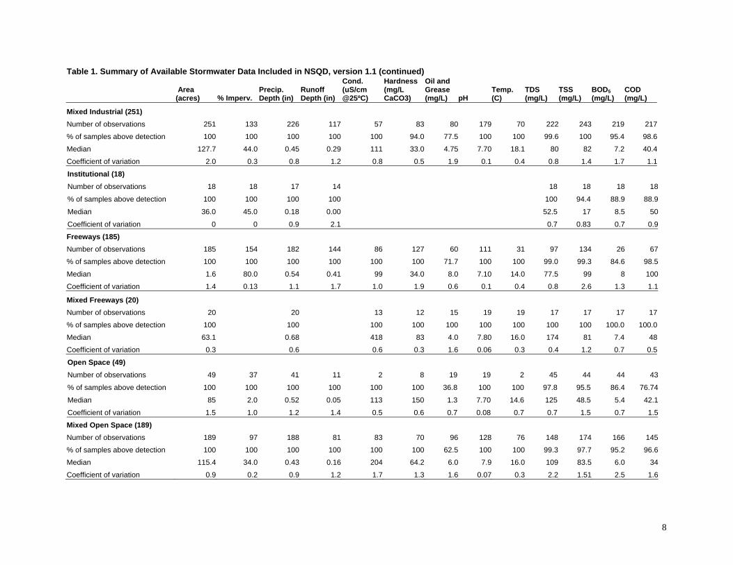
verification during the QA/QC process. If that potentially faulty data remained in the database, spurious statistical analyses would have resulted. The collection and review of the data is a necessary first step to facilitate later analyses. The assembled data was entered into NSQD, including site descriptions (state, municipality, land use components, and EPA rain zone), sampling information (date, season, rain depth, runoff depth, sampling method, sample type, etc.), and constituent measurements (concentrations, grouped in categories). In addition, more detailed site, sampling, and analysis information has been collected for most sampling sites and is also included as supplemental information. The reported land use information supplied by the communities is being used, with verification of some areas with aerial photographs and maps. In many cases, the sampled watersheds have multiple land uses and those designations are included in the database (the database lists the percentages of the drainage as residential, commercial, industrial, freeway, institutional, and open space). The final data analyses will consider these mixed sites also, especially for verification for the model development activities, although the following preliminary results are only for the homogeneous land use sites. Preliminary Summary of U.S. NPDES Phase 1 Stormwater Data Additional site information is being acquired to complete most of the missing records before the final data analyses. The following data and analysis descriptions should therefore be considered preliminary and will change with this additional data and analyses. However, this presentation only uses the most basic and robust analyses for preliminary consideration. The final report and data presentations will obviously be much more comprehensive. Table 1 is a summary of the Phase 1 data collected and entered into the database as of mid-summer 2003. The data are separated into 11 land use categories: residential, commercial, industrial, institutional, freeways, and open space, plus mixtures of these land uses. Summaries are also shown for mixed land use areas (indicating the most prominent land use), and for the total data set combined. Only data having at least 50 total detected observations and at least 10 detected observations per land use category are shown on this table. The full database includes all of the data. In most cases, many more than these minimum numbers are available. The total number of observations and the percentage of observations above the detection limits are also shown on this summary table. However, some constituents were not monitored by very many stormwater permit holders, and some constituents were mostly all in the “not detected” category, and those data are not shown. As an example, filtered heavy metal observations, and especially organic analyses, have many fewer detected values than other constituents. The total number of individual events included in the database is 3,770, with most in the residential category (1,069 events). For most common constituents, detectable values are available for almost all monitored events. The median and coefficient of variation (COV) values are only for those data having detectable concentrations. If the non-detected results were used in these calculations, extreme biases would invalidate many of the calculations. The final analyses will further examine issues associated with different detection limits, multiple laboratories, and varying analytical methods on the reported results and statistical analyses. Burton and Pitt (2002), and the many included references in that book, contains further discussions on these important issues.
6
Figure 1. Communities from which data has been obtained and entered in the NSQD, along with EPA Rain Zones. Table 2 is a summary of methylene chloride and bis(2-ethylhexyl) phthalate, the most commonly reported and detected organic constituents. There were up to several hundred events that included PAH and pesticide data. The percentage of samples that had observable concentrations of these constituents ranged from 15 to 35%, about the same detection rate as in previous stormwater investigations, such as Pitt, et al. 1995. Statistical analyses are being conducted in stages. Probability plots were used to identify range, randomness, and normality. Figure 2 is an example of log-normal probability plots for some of the constituents and for all data pooled. Probability plots shown as straight lines indicate that the concentrations can be represented by log-normal distributions. This is important as it indicates that data transformations, or the use of nonparametric statistical analyses, will be needed. Plots with obvious discontinuities imply that multiple data populations may be included. The future analyses will identify the significance of these different data categories (such as land use, region, and season).
7
Table 1. Summary of Available Stormwater Data Included in NSQD, version 1.1
Area (acres) % Imperv.
Precip. Depth (in)
Runoff Depth (in)
Cond. (uS/cm @25ºC)
Hardness (mg/L CaCO3)
Oil and Grease (mg/L) pH
Temp. (C)
TDS (mg/L)
TSS (mg/L)
BOD5 (mg/L)
COD (mg/L)
Overall Summary (3765) Number of observations 3759 2202 3186 1454 685 1082 1834 1665 861 2957 3390 3105 2751
Figure 2. Log-normal probability plots of stormwater quality data for selected constituents.
14
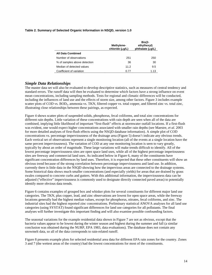
Table 2. Summary of Selected Organic Information in NSQD, version 1.0
Methylene-
chloride (µg/L)
Bis(2-ethylhexyl)
phthalate (µg/L) All Data Combined Number of observations 251 250 % of samples above detection 36 30 Median of detected values 11.2 9.5 Coefficient of variation 0.77 1.13
Simple Data Relationships The master data set will also be evaluated to develop descriptive statistics, such as measures of central tendency and standard errors. The runoff data will then be evaluated to determine which factors have a strong influence on event mean concentrations, including sampling methods. Tests for regional and climatic differences will be conducted, including the influences of land use and the effects of storm size, among other factors. Figure 3 includes example scatter plots of COD vs. BOD5, ammonia vs. TKN, filtered copper vs. total copper, and filtered zinc vs. total zinc, illustrating close relationships between these pairings, as expected. Figure 4 shows scatter plots of suspended solids, phosphorus, fecal coliforms, and total zinc concentrations for different rain depths. Little variation of these concentrations with rain depth are seen when all of the data are combined, implying little likelihood of important “first-flush” effects at stormwater outfall locations. If a first-flush was evident, one would expect higher concentrations associated with smaller rain depths (see Maestre, et al. 2003 for more detailed analyses of first-flush effects using the NSQD database information). A simple plot of COD concentrations vs. percentage imperviousness of the drainage area (Figure 5) doesn’t indicate any obvious trends. Each vertical set of observations represent a single monitoring location (all of the events at a single location have the same percent imperviousness). The variation of COD at any one monitoring location is seen to vary greatly, typically by about an order of magnitude. These large variations will make trends difficult to identify. All of the lowest percentage imperviousness sites are open space land uses, while all of the highest percentage imperiousness sites are freeway and commercial land uses. As indicated below in Figure 6, many of the constituents have significant concentration differences by land uses. Therefore, it is expected that these other constituents will show an obvious trend because of the strong correlation between percentage imperviousness and land use. In addition, currently there is little data in the NSQD showing how the impervious areas are connected to the drainage systems. Some historical data shows much smaller concentrations (and especially yields) for areas that are drained by grass swales compared to concrete curbs and gutters. With this additional information, the imperviousness data can be adjusted (“effective” imperviousness is commonly used to designate directly connected paved areas) to potentially identify more obvious data trends. Figure 6 contains examples of grouped box and whisker plots for several constituents for different major land use categories. The TKN, plus copper, lead, and zinc observations are lowest for open space areas, while the freeway locations generally had the highest median values, except for phosphorus, nitrates, fecal coliforms, and zinc. The industrial sites had the highest reported zinc concentrations. Preliminary statistical ANOVA analyses for all land use categories (using SYSTAT) found significant differences for land use categories for all pollutants. The final analyses will further investigate this important finding and will also examine possible confounding factors. The seasonal variations for the example residential data shown in Figure 7 are not as obvious, except that the bacteria values appear to be lowest during the winter season and highest during the summer and fall (a similar conclusion was obtained during the NURP, EPA 1983, data evaluations). The database does not contain any snowmelt data, so all of the data corresponds to rain-related runoff. Figure 8 presents example plots for selected residential area data for different EPA rain zones for the country. Zones 3 and 7 (the wettest areas of the country) had the lowest concentrations for most of the constituents.
15
Figure 3. Example scatter plots of stormwater data (line of equivalent concentration shown).
16
Figure 4. Example scatter plots of concentrations vs. rain depth.
17
Figure 5. Plot COD concentrations against watershed area percent imperviousness values for different land uses (CO: commercial; FW: freeway; ID: industrial; OP: open space; and RE: residential)
18
Figure 6. Example stormwater data sorted by land use (no mixed land use data included in plots).
19
Figure 6. Example stormwater data sorted by land use (no mixed land use data included in plots) (continued).
20
Figure 7. Example residential area stormwater pollutant concentrations sorted by season.
21
Figure 8. Example residential area stormwater pollutant concentrations sorted by geographical area. We are also examining trends of concentrations with time. A classical example would be for lead, which is expected to decrease over time with the increased use of unleaded gasoline. Older stormwater samples from the 1970s typically have had lead concentrations of about 100 µg/L, or higher, while most current data indicate concentrations in the range of 1 to 10 µg/L. Figure 9 shows a plot of lead concentrations for residential areas only (in rain zone 2), for the time period from 1991 to 2002. This preliminary plot shows likely decreasing lead concentrations with time. Statistically however, the trend line is not significant due to the large variation in observed concentrations (p=0.41; there is insufficient data to show that the slope term is significantly different from zero). The similar COD concentrations in Figure 9 also have an apparent downward trend with time, but again, the slope term is not significant (p=0.12).
22
Figure 9. Residential lead and COD concentrations with time (EPA Rain Zone 2 data only). As part of their MS4 phase 1 applications, Denver and Milwaukee both returned to some of their earlier sampled monitoring stations used during the local NURP projects. In the time between the early 1980s (NURP) and the early 1990s (MS4), they did not detect any significant differences, except for large decreases in lead concentrations. Figure 10 compares suspended solids, copper, lead, and zinc concentrations at the Wood Center NURP monitoring site in Milwaukee. The average site concentrations remained the same, except for lead, which decreased from about 450 down to about 110 µg/L.
Figure 10. Comparison of pollutant concentrations collected during NURP (1981) to MS4 application data (1990) at the same location (personal communication, Roger Bannerman, WI DNR). Similar comparisons were made in the Denver Metropolitan area by the Urban Drainage and Flood Control District. Table 3 compares stormwater quality for commercial and residential areas for 1980/91 (NURP) and 1992/93 (MS4 application). Although there was an apparent difference in the averages of the event concentrations between the sampling dates, they concluded that the differences were all within the normal range of stormwater quality variations, except for lead, which decreased by about a factor of four.
23
Table 3. Comparison of Commercial and Residential Stormwater Runoff Quality from 1980/81 to 1992/93 (Urban Drainage District, Flood Hazard News, Dec 1993.)
Commercial Residential Constituent 1980/81 1992/93 1980/82 1992/93 Total suspended solids (mg/L) 251 165 226 325 Total nitrogen (mg/L) 3.0 3.9 3.2 4.7 Nitrate plus nitrite (mg/L) 0.80 1.4 0.61 0.92 Total phosphorus (mg/L) 0.46 0.34 0.61 0.87 Dissolved phosphorus (mg/L) 0.15 0.15 0.22 0.24 Copper, total recoverable (µg/L) 27 81 28 31 Lead, total recoverable (µg/L) 200 59 190 53 Zinc, total recoverable (µg/L) 220 290 180 180
Example Statistical Analyses of Data Comparing First Flush and Composite Sample Concentrations As part of their NPDES stormwater permit, some communities collected grab samples during the first 30 minutes of the event to evaluate a “first flush” in contrast to the flow-weighted composite data. More than 400 paired samples representing the first flush and composite samples from eight communities (mostly located in the southeast U.S.) from NSQD were reviewed. Box and probability plots were prepared for 22 major constituents. Nonparametric statistical analyses were then used to measure the differences between the sample sets. This discussion summarizes the results of this preliminary analysis, including the effects of storm size and land use on the presence and importance of first flushes. Only concentration data were available for these analyses, so traditional accumulative mass curves could not be developed. First flush refers to an assumed elevated load of pollutants discharged in the first part of a runoff event. First flush has been observed more in small catchments than in large catchments (Thompson, et al. 1995; WEF and ASCE 1998). In large catchments (>162 ha, or >400 acres) the highest concentrations have been observed at the times of flow peak (Soeur, et al. 1994; Brown, et al. 1995). The presence of a first flush has been reported to be associated with runoff duration by the City of Austin, TX (Swietlik, et al. 1995). An observed first flush may be present for some pollutants, but not others (Ellis 1986; Adams 2000). Adams (2000) and Deletic (1998) both concluded that the presence of a first flush depends on numerous site and rainfall characteristics. It is expected that peak concentrations generally occur during periods of peak flow (and highest rain energy). On relatively small paved areas, however, it is likely that there will always be a short period of relatively high concentrations associated with washing off of the most available material near the beginning of the runoff event (Pitt 1987). This peak period of high concentrations may be overwhelmed by periods of high rain intensity that may occur later in the event. In addition, in more complex drainage areas, the routing of these short periods of peak concentrations may blend with larger flows and may not be noticeable. A first flush in a separate storm drainage system is therefore most likely to be seen if a rain occurs at relatively constant intensity over a paved area having a simple and small drainage system. A total of 417 storm events with paired first flush and composite storm samples were available from the NSQD. The majority of the events were located in North Carolina (76.2%), but some events were also from Alabama (3.1%), Kentucky (13.9%) and Kansas (6.7%). All of the data were from end-of pipe samples in separate storm drainage systems. The initial analyses were used to select the constituents and land uses that meet the requirements of the statistical comparison tests. Probability plots, box plots, concentration vs. precipitation, and standard descriptive statistics, were performed for 22 constituents for each land use, and for all land uses combined. Nonparametric statistical analyses were performed after the initial analyses. Mann Whitney and Fligner Policello tests were most commonly used. Minitab and Systat statistical programs, along with Word and Excel macros, were used for the analyses. The Mann-Whitney and Fligner-Policello non-parametric tests were selected to determine if there were statistically significant differences between the first flush and composite data sets for each land use and constituent. These tests are very useful because they require only data symmetry, not normality, to evaluate the hypothesis. The null hypothesis during the analysis was that the median concentrations of the first flush and composite data sets were the same. The alternative hypothesis was that the medians were different, with a confidence of at least 95%.
24
A complete description of these analyses is presented in Maestre, et al. (2004). Table 4 summarizes the results of the analysis. The “>” sign indicates that the median of the first flush data set is higher than for the composite storm data set. The “=” sign indicates that the there is not enough information to reject the null hypothesis. Events without enough data for the analyses are represented with an “X”. Also shown on this table are the ratios of the medians of the first flush and the composite data sets for each constituent and land use. The first flush samples were larger than for the composite samples if the ratio is great than one. Generally, a statistically significant first flush is associated with a median concentration ratio of about 1.4, or greater (the exceptions occurred when the number of samples in a specific category is small). The largest significant ratios are about 2.5, indicating that the first flush concentrations may be about 2.5 times greater than the composite concentrations. More of the larger ratios are found in the commercial and institutional land use categories, areas where larger paved areas are likely to be found. The smallest ratios are associated with the residential, industrial, and open space land uses, locations where there may be larger areas of unpaved surfaces. Results indicate that for 55% of the evaluated cases, the medians of the first flush data sets were significantly larger than for the composite sample sets. In the remaining 45% of the cases, both medians were expected to be the same, or the concentrations were possibly greater later in the events. About 70% of the constituents in the commercial land use category had first-flushes, while about 60% of the constituents in the residential, institutional and the mixed (mostly commercial and residential) land use categories had first flushes, and about 45% of the constituents in the industrial land use category had first-flushes. In contrast, no constituents were found to have first-flushes in the open space category. COD, BOD5, TDS, TKN, and Zn all had first flushes in all areas (except for the open space category). In contrast, turbidity, pH, fecal coliforms, fecal strep., total N, dissolved and ortho-P never showed a statistically significant first flush in any category. The conflict with TKN and total N implies that there may be some other factors involved in the identification of first flushes besides land use. If additional paired data become available during later project periods, it may be possible to extend these analyses to consider rain effects, drainage area, and geographical location. Table 4. Presence of Significant First Flushes (ratio of first flush to composite median concentrations)
Parameter Commercial Industrial Institutional Open Space Residential All Combined
Turbidity = (1.32) X X X = (1.24) = (1.26) pH = (1.03) = (1.00) X X = (1.01) = (1.01) COD > (2.29) > (1.43) > (2.73) = (0.67) > (1.63) > (1.71) TSS > (1.85) = (0.97) > (2.12) = (0.95) > (1.84) > (1.60) BOD5 > (1.77) > (1.58) > (1.67) = (1.07) > (1.67) > (1.67) TDS > (1.82) > (1.32) > (2.66) = (1.07) > (1.52) > (1.55) O&G > (1.54) X X X = (2.05) > (1.60) Fecal Coliform = (0.87) X X X = (0.98) = (1.21) Fecal Strep. = (1.05) X X X = (1.30) = (1.11) Ammonia > (2.11) = (1.08) > (1.66) X > (1.36) > (1.54) NO2 NO3 > (1.73) > (1.31) > (1.70) = (0.96) > (1.66) > (1.50) Total N = (1.35) = (1.79) X = (1.53) = (0.88) = (1.22) TKN > (1.71) > (1.35) X = (1.28) > (1.65) > (1.60) Total P > (1.44) = (1.42) = (1.24) = (1.05) > (1.46) > (1.45) P Dissolved = (1.23) = (1.04) = (1.05) = (0.69) > (1.24) = (1.07) Phosphate Ortho X = (1.55) X X = (0.95) = (1.30) Cd > (2.15) = (1.00) X = (1.30) > (2.00) > (1.62) Cr > (1.67) = (1.36) X = (1.70) = (1.24) > (1.47) Cu > (1.62) > (1.24) = (0.94) = (0.78) > (1.33) > (1.33) Pb > (1.65) > (1.41) > (2.28) = (0.90) > (1.48) > (1.50) Ni > (2.40) = (1.00) X X = (1.20) > (1.50) Zn > (1.92) > (1.540 > (2.48) = (1.25) > (1.58) > (1.59)
25
Modeling Building using the NSQD As indicated earlier, an important objective of the NSQD is to develop a predictive tool to enable stormwater managers to determine the likely stormwater quality for their area. In many cases, adequate data may be available in the NSQD to fit their situation. However, it is also expected that some will need to establish a local monitoring program to obtain reliable estimates of their stormwater quality. The next subsection provides some monitoring guidance for this situation, while this subsection presents an example of the model building process that we are currently using. Factors Potentially Affecting Stormwater Pollutant Concentrations The database contains information for the monitored watersheds, along with the outfall runoff quality. Each sample is labeled with the land use, season, geographical area, percent imperviousness, rain amount, and many other attributes in the database. The first phase of the NSQD project focused on the mid Atlantic and Gulf coast areas, although additional data has been collected for other locations. About 54% of the existing data in the database is from communities located in Maryland, Virginia, Pennsylvania, North Carolina, Kentucky and Tennessee. The following factors may affect the reported stormwater pollutant concentrations:
• Landuse: All of the watershed areas were separated into residential, commercial, industrial, open space and freeway land uses. Data are also available from mixed landuse areas which will be used later to verify the prediction methods.
• EPA Rain Zone: As shown in Figure 1, the country is divided in 9 rain/climatic regions representing all combinations of areas having warm summers, cold winters, large rainfalls, and little rain.
• Season: Four seasons were identified by the month when the samples were collected: Winter (December to February); Spring (March to May); Summer (June to August); and Fall (September to November).
• Percentage Imperviousness: About 2/3 of the monitoring sites currently have percentage imperviousness data.
• Rainfall: Almost all of the events have the rainfall amount associated with the monitored event. • Type of sample collection: Some of the events represent special “first-flush” and composite sample pairs
for the same event. These data were evaluated previously to identify these effects on runoff water quality. The type of sampler and sampling method has been identified for about ¼ of the sampling locations.
• Runoff amount: About 1/3 of the events have the runoff amounts associated with the monitored events. • Watershed area: All of the monitored locations have the watershed areas identified. • Date of sample collection: All of the data are associated with the date of sample collection. In addition to
the seasonal effects, this information can be used to examine any trends in concentration that may have occurred during the 10 years of sample collection represented in the NSQD.
• Type of conveyance system: About 1/3 of the sites have the conveyance system identified. • Aerial photographs and topographic maps have been obtained for almost all of the monitoring areas.
Figure 11 is a probability plot for the observed COD concentrations separated by land use. This plot is similar to the previously presented box and whisker plots for the different constituents separated by land use. These plots do show additional information that is useful for developing predictive models. As typically assumed, the COD values closely follow log-normal probability plots for much of the data range (Figure 2 illustrates log-normal probability plots for many of the constituents available in the NSQD, but grouped for all factors combined). Figure 11 shows significant differences by land uses. The open space COD concentrations are the lowest, and the freeway COD concentrations are the largest for most all of the data range. The residential, commercial, and industrial areas are very similar for the lower half of the distribution, while the residential areas are lower than the commercial and industrial areas in the upper portion of the distribution. The effects of some of the above listed factors on concentrations have been previously illustrated. The following shows how we plan to develop the predictive tool for the main watershed factors listed above. In this example, we will examine COD concentrations as a function of EPA rain zones and season, for the residential areas.
26
Figure 11. Probability plots of COD concentrations for different land uses. It is possible to identify statistically significant differences in the COD concentrations for residential land uses in different EPA zones and seasons. Table 5 shows the total number of storm events collected which has residential COD values for the different rain zones and seasons. Table 5. Number of Events with Detected COD Values in Residential Land Use Areas in the NSQD
Table 5 shows that EPA rain zone 2 has about 62% of the total number of COD observations in the database. This unbalance of sample numbers can potentially lead to confusing results if the other areas do not adequately represent the actual conditions in their areas and is a violation of the data assumptions needed for a successful ANOVA test. It is possible to see if there is a difference in the COD concentrations for the different seasons in each zone during the four seasons using a one-way analysis of variance test, as the numbers of samples in each season for each main zone are relatively even. The analysis of variance requires that the residuals are normally distributed and there is the same variance for each of the seasons. After log transforming the data, it was found that the residuals can be considered normal with a p-
27
value of 0.8 using the Kolmogorov-Smirnov Goodness of fit test. To test if the variances are the same for the four seasons, Barlett’s test was used. This test is powerful when the normality assumption of the residuals is achieved, as in this example. The results indicated that the variance can be considered the same for each season in EPA rain zone 2, with a p-value of 0.44. The results of the ANOVA found that there is a significant difference in the COD concentrations during the four seasons. The COD concentration in EPA rain zone two during winter seems to be smaller than summer and spring. The pooled standard deviation of the observations was calculated as 0.677 Power Calculations as a Function of Numbers of Data Observations Figure 12 is a set of power curves showing the difference in the mean COD concentrations for the different subgroups that can be identified for different numbers of samples. If the ANOVA test indicated a significant difference with a confidence of five percent (α=0.05), these mean differences can be detected for the noted sample sizes. Table 6 lists the sample sizes needed, for a power level of 0.8 and a confidence of 0.05, to detect the noted differences in mean concentrations. If a goal of at least a 25% difference was desired, then about 120 samples in each season would be needed. This is approximately the conditions for EPA rain zone 2 residential land uses. However, if only 10 samples are available for each season, then the “detectable” difference would be relatively large (larger than 50%).
5 10 20 25 30 40 50
0 25 50 75 100 125 150 175 200 225
0.0
0.2
0.4
0.6
0.8
1.0
Size
Pow
er
percentage difference among seasonsArea for EPA Zone 2. Samples Required to detect aPower of the ANOVA. COD Concentration in Residential
Figure 12. Power of the one way ANOVA test for COD in EPA rain zone 2. Table 6. Samples required to detect specific differences in the COD for different seasons
Percentage difference between the mean values
(%)
Samples Required
5 3844 10 908 20 202 25 122 30 80 40 40 50 22
28
Multivariate Analyses of Factors A two-way analysis can also be conducted to examine the effects of both seasons and rain zones together, and their interaction. In the following example, rain zones 3, 4, 5, 6, and 7 were evaluated for all four seasons. Rain zone 2 was excluded from this preliminary analysis because it had many more samples than the other regions and could have overly emphasized those conditions. The first step in this analysis is to check the distributions and variances of the data sets. The residuals (the differences of the observations from the mean) can be considered normal as they had a p-value higher than 15% (no significant difference from a normal distribution). Barlett’s test also indicated that the variance for the different groups can be considered the same with a p-value of 0.35. A two-way ANOVA can therefore be used to identify any differences between the seasons and EPA rain zones, plus their interaction, because the data were normally distributed and they have the same variance within each group. The 2-way ANOVA results indicated that there are no significant differences between the different seasons (p-value = 0.091), but that there is a difference between the EPA rain zones (p-value < 0.001). Figure 13 contains probability plots of the residential COD values for each season, showing no clear distinction of these concentrations for the different seasons. The ANOVA test also found no significant interaction between rain zone and season (p-value = 0.25).
Figure 13. Probability plots of residential COD concentrations for different seasons. Figure 14 shows probability plots of residential area COD concentrations for each EPA rain zone. There are likely three distinct groupings for residential COD values, based on their geographical location. Samples collected in zone 6 had the highest mean concentrations and were collected in Arizona. Samples collected in zones 2, 4 and 5 were intermediate in COD concentration and were collected in the mid Atlantic states and Texas. Samples collected in zones 3 and 7 had the lowest COD concentrations and were collected in Alabama, Georgia, and in Oregon.
29
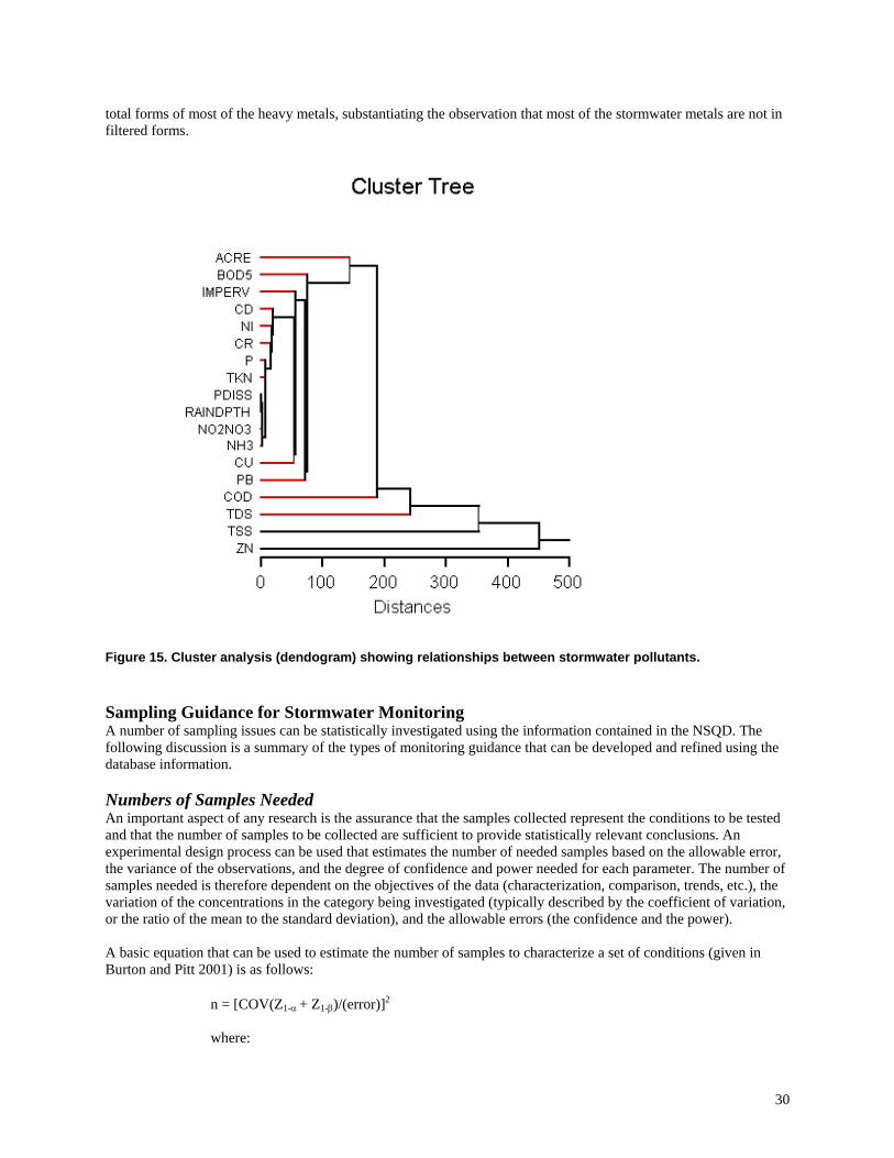
Figure 14. Probability plots of residential COD concentrations in different EPA Ran Zones. Therefore, COD residential area concentrations can be divided into the following three groups, based on EPA rain zone: Zones 3 and 7: average: 44.4 mg/L, standard deviation: 41.9 (102 observations) Zones 2, 4 and 5: average: 72.8 mg/L, standard deviation: 61.6 (628 observations) Zone 6: average: 162.1 mg/L, standard deviation: 100.0 (44 observations) Overall residential COD: average: 74.1, standard deviation: 69.2 mg/L The statistical analyses of the available NSQD COD residential area data did not identify any significant differences in any rain zones that can be explained by season. There was insufficient data in zones 1, 8, and 9 to be evaluated by season and the overall residential COD values should therefore be used for those areas until additional data is collected and evaluated. Clustering and principal component analyses (PCA) are also being used to identify expected factors influencing sample variability. Figure 15 is an example dendogram from a cluster analysis of all of the preliminary data combined. However this analysis did not include most of the site characteristics when it was conducted; only rain depth, watershed size, and percentage imperviousness were included for this analysis, in addition to the runoff concentrations. This plot indicates very close relationships between rain depth and the nutrients (total phosphorus, dissolved phosphorus, nitrite plus nitrate, ammonia, and Total Kjeldahl Nitrogen). Some of the heavy metals (cadmium, nickel, and chromium) are closely related to each other, but copper, lead and zinc are much more independent. BOD5, COD, dissolved solids, and suspended solids are poorly related to other pollutants for the pooled data. Pearson correlation analyses did show relatively strong relationships between suspended solids and the
30
total forms of most of the heavy metals, substantiating the observation that most of the stormwater metals are not in filtered forms.
Figure 15. Cluster analysis (dendogram) showing relationships between stormwater pollutants. Sampling Guidance for Stormwater Monitoring A number of sampling issues can be statistically investigated using the information contained in the NSQD. The following discussion is a summary of the types of monitoring guidance that can be developed and refined using the database information. Numbers of Samples Needed An important aspect of any research is the assurance that the samples collected represent the conditions to be tested and that the number of samples to be collected are sufficient to provide statistically relevant conclusions. An experimental design process can be used that estimates the number of needed samples based on the allowable error, the variance of the observations, and the degree of confidence and power needed for each parameter. The number of samples needed is therefore dependent on the objectives of the data (characterization, comparison, trends, etc.), the variation of the concentrations in the category being investigated (typically described by the coefficient of variation, or the ratio of the mean to the standard deviation), and the allowable errors (the confidence and the power). A basic equation that can be used to estimate the number of samples to characterize a set of conditions (given in Burton and Pitt 2001) is as follows: n = [COV(Z1-α + Z1-β)/(error)]2
where:
31
n = number of samples needed
α= false positive rate (1-α is the degree of confidence. A value of α of 0.05 is usually considered statistically significant, corresponding to a 1-α degree of confidence of 0.95, or 95%.)
β= false negative rate (1-β is the power. If used, a value of β of 0.2 is
common, but it is frequently and improperly ignored, corresponding to a β of 0.5.) Z1-α = Z score (associated with area under normal curve) corresponding to
1-α. If α is 0.05 (95% degree of confidence), then the corresponding Z1-α score is 1.645 (from standard statistical tables).
Z1-β= Z score corresponding to 1-β value. If β is 0.2 (power of 80%), then the corresponding Z1-β score is 0.85 (from standard statistical tables). However, if power is ignored and β is 0.5, then the corresponding Z1-β score is 0.
error = allowable error, as a fraction of the true value of the mean COV = coefficient of variation (sometimes noted as CV), the standard deviation
divided by the mean (Data set assumed to be normally distributed.) This equation assumes a normal distribution of the data, which would require a log transformation of most stormwater quality data. If an allowable error of about 25% is desired and the COV is estimated to be 0.4, then about 20 samples would have to be analyzed. The use of stratified random sampling can usually be used to advantage by significantly reducing the COV of the sub-population in the strata, requiring fewer samples for characterization. Typical Numbers of Samples Needed for a Basic Stormwater Monitoring Program The COV values for many constituents shown in Table 1 for the NPDES database range from unusually low values of about 0.1 (for pH) to highs between 1 and 2. There are a few COV values that are larger. One objective of a data analysis procedure is to categorize the data into separate stratifications, each having small variations in the observed concentrations. The only stratification in Table 1 is land use. However, Figure 6 shows many differences by geographical area (refer to Figure 1 for the EPA Rain Zone map). It is expected that the final data analyses for this project will identify separate stratifications of data (possibly considering the combination of land use, geographical area, and season factors) to significantly reduce the variations in each category. It is expected that COV values in the range of 0.5 to 1.0 will be common for many of these data stratifications. With a reasonable confidence of 95% (α= 0.05) and power of 80% (β= 0.20), and a commonly accepted allowable error of 25%, the number of samples needed to characterize conditions would likely range from about 25 to 50. If only 12 samples are obtained for each category (strata), the allowable errors would range from about 50% to 100%. Burton and Pitt (2001) present many additional experimental design equations and plots for other data quality objectives, including the effects of log transforming the data for more appropriate sampling effort approximations. In many cases, the actual errors in presenting data are larger than expected, due to relatively small numbers of samples. A continuing monitoring program (such as the Phase I stormwater NPDES permit monitoring effort) will result in better data as more samples are obtained with time. Detection Limits of Analytical Methods The NSQD can also be useful when selecting analytical methods. There are many important factors that must be considered when selecting an analytical method (availability, cost, detection limit, repeatability, safety and disposal problems, comparisons with historical data, etc.), but the detection limit is likely most important when ensuring the suitability of the data. In many cases, analytical methods are used that have detection limits that are actually larger than a criterion value, making accurate exceedence frequencies impossible (Burton and Pitt 2001).
32
Environmental researchers need to be concerned with many attributes of numerous analytical methods when selecting the most appropriate methods to use for analyses of their samples. The main factors that affect the selection of an analytical method include: cost, reliability (the “data quality objectives,” or DQO which includes sensitivity, selectivity, repeatability), and safety. Most of these issues are not well documented in the literature for environmental sample analyses. Aspects of analytical reliability have received the most attention in the literature, but most of the other aspects noted above have not been adequately discussed for the many analytical alternatives available. It is therefore difficult for a water quality analyst to decide which methods to select, or even if a choice exists. The selection of the appropriate analysis procedure is dependent on the use of the data and how false negatives or false positives would affect water use decisions or regulatory questions. The QA objectives for the method detection limit (MDL) and precision (RPD) for the compounds of interest have been shown to be a function of the anticipated median concentrations in the samples (Pitt, et al. 1993). The MDL objectives should generally be about 0.25, or less, of the median value for sample sets having typical concentration variations (COV values ranging from 0.5 to 1.25), based on many Monte Carlo evaluations to examine the rates of false negatives and false positives. Table 7 lists the typical median stormwater runoff constituent concentrations and the associated calculated MDL goals, for a typical stormwater monitoring project. Using analytical methods having these detection limits, at least, will result in relatively few “non-detected” values. In most cases, analytical methods are available that can easily meet these goals. However, common problems are associated with some of the heavy metals, as most modern laboratories use ICP (inductively-coupled plasma) instruments that are capable of analyzing a broad range of metals simultaneously, but may not be able to meet these detection limit goals. When dissolved forms of the heavy metals need to be analyzed, the detection limits must be much smaller. The NPDES stormwater database can be used to indicate the likely concentrations of interest for conditions similar to those that will be monitored. These expected values are a good start in determining the needed detection limits. Sampling Methods Details for all monitoring locations are desired for the database. Basic information (land use, season, geographic location, and if the sample is a first-flush or a composite sample) is available for all events in NSQD, and relatively complete site and monitoring descriptions are available for about 1/3 of the events. This data includes sampling methods (automatic samplers vs. manual samplers; manufacture and model of sampler; etc.). Investigations of how these factors may influence the monitoring results will be made, as illustrated in the initial evaluation of first-flush vs. composited samples. The effects of automatic vs. manual sampling will also be examined when sufficient information has been collected. One example of a previous investigation on stormwater sampling methods was conducted by Roa-Espinosa and Bannerman (1995). They collected samples from five industrial sites using different monitoring methods. They concluded that many time-composited subsamples combined for a single analysis can provide improved accuracy compared to fewer samples associated with flow-weighted samplers, and especially compared to samples only taken during a portion of an event. Conclusions A major goal of this project is to provide guidance to stormwater managers and regulators. Especially important will be the use of this data as an updated benchmark for comparison with locally collected data. These comparisons will enable local monitoring data to be compared to typical values that should be expected for similar situations. If the local stormwater quality is significantly worse than expected, then it may be possible to quantify a treatment goal that should be attainable. In addition, this data may be useful for preliminary calculations when using the “simple method” for predicting mass discharges for unmonitored areas. This data can also be used as guidance when designing local stormwater monitoring programs (Burton and Pitt 2002), especially when determining the needed sampling effort based on expected variations. The final data analyses will expand on these preliminary examples and will also investigate other stormwater data and sampling issues.
33
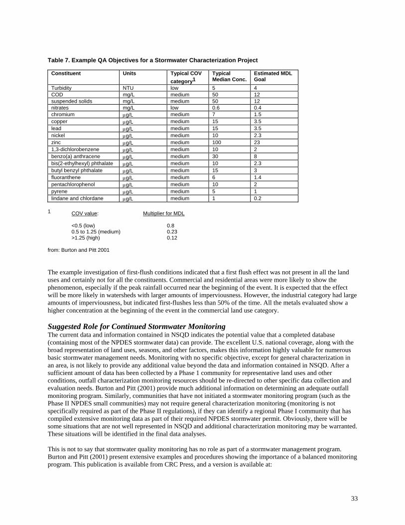
Table 7. Example QA Objectives for a Stormwater Characterization Project
Constituent Units Typical COV
category1 Typical Median Conc.
Estimated MDL Goal
Turbidity NTU low 5 4 COD mg/L medium 50 12 suspended solids mg/L medium 50 12 nitrates mg/L low 0.6 0.4 chromium µg/L medium 7 1.5 copper µg/L medium 15 3.5 lead µg/L medium 15 3.5 nickel µg/L medium 10 2.3 zinc µg/L medium 100 23 1,3-dichlorobenzene µg/L medium 10 2 benzo(a) anthracene µg/L medium 30 8 bis(2-ethylhexyl) phthalate µg/L medium 10 2.3 butyl benzyl phthalate µg/L medium 15 3 fluoranthene µg/L medium 6 1.4 pentachlorophenol µg/L medium 10 2 pyrene µg/L medium 5 1 lindane and chlordane µg/L medium 1 0.2
1 COV value: Multiplier for MDL <0.5 (low) 0.8 0.5 to 1.25 (medium) 0.23 >1.25 (high) 0.12 from: Burton and Pitt 2001 The example investigation of first-flush conditions indicated that a first flush effect was not present in all the land uses and certainly not for all the constituents. Commercial and residential areas were more likely to show the phenomenon, especially if the peak rainfall occurred near the beginning of the event. It is expected that the effect will be more likely in watersheds with larger amounts of imperviousness. However, the industrial category had large amounts of imperviousness, but indicated first-flushes less than 50% of the time. All the metals evaluated show a higher concentration at the beginning of the event in the commercial land use category. Suggested Role for Continued Stormwater Monitoring The current data and information contained in NSQD indicates the potential value that a completed database (containing most of the NPDES stormwater data) can provide. The excellent U.S. national coverage, along with the broad representation of land uses, seasons, and other factors, makes this information highly valuable for numerous basic stormwater management needs. Monitoring with no specific objective, except for general characterization in an area, is not likely to provide any additional value beyond the data and information contained in NSQD. After a sufficient amount of data has been collected by a Phase 1 community for representative land uses and other conditions, outfall characterization monitoring resources should be re-directed to other specific data collection and evaluation needs. Burton and Pitt (2001) provide much additional information on determining an adequate outfall monitoring program. Similarly, communities that have not initiated a stormwater monitoring program (such as the Phase II NPDES small communities) may not require general characterization monitoring (monitoring is not specifically required as part of the Phase II regulations), if they can identify a regional Phase I community that has compiled extensive monitoring data as part of their required NPDES stormwater permit. Obviously, there will be some situations that are not well represented in NSQD and additional characterization monitoring may be warranted. These situations will be identified in the final data analyses. This is not to say that stormwater quality monitoring has no role as part of a stormwater management program. Burton and Pitt (2001) present extensive examples and procedures showing the importance of a balanced monitoring program. This publication is available from CRC Press, and a version is available at:
34
http://civil.eng.ua.edu/~rpitt/Publications/BooksandReports/Stormwater%20Effects%20Handbook%20by%20%20Burton%20and%20Pitt%20book/MainEDFS_Book.html Stormwater quality monitoring is a crucial component of local programs. Specific objectives for these include: • Receiving water assessments to understand local problems. Receiving water monitoring is needed to identify local problems, especially when identifying beneficial use impairments. Assimilative capacity calculations (TMDLs) require knowledge of local source discharges. The NSQD data and information can be used for preliminary designs and cost estimates, but it is also important to invest a small amount of resources to accurately determine local discharge conditions before expensive controls are designed. • Source area monitoring to identify critical sources. In many cases, source area controls may be more cost-effective than regional controls. The identification of critical source areas is therefore needed as part of a comprehensive stormwater management program. Monitoring within a critical drainage area should be conducted to identify the sources of pollutants, while simultaneous outfall monitoring is needed to verify these source area measurements. • Detailed monitoring at selected outfalls, with complete monitoring of rainfall and runoff, with high-resolution data to examine time-variability characteristics of certain problem pollutants. This would be especially important at small, highly paved areas where “first-flush” conditions are most likely. This information is needed to evaluate the benefits and to quantify design approaches of critical source area controls. • Treatability tests to verify performance of stormwater controls for local conditions. In areas where stormwater controls are being installed, local measurements of performance are a good investment. Before and after monitoring, or parallel monitoring, is usually needed to measure the performance of many types of stormwater controls. The ASCE National Stormwater BMP database (http://www.bmpdatabase.org/) is a good place to start in predicting the performance of controls, but site-specific validations in an area where the controls have not been previously used should be conducted. • Assessment monitoring to verify success of stormwater management approach. Stormwater quality monitoring is a critical component of an assessment monitoring effort. Receiving water monitoring needs to focus on beneficial use impairments, and associated chemical, physical, and biological monitoring. In many cases, source area or outfall controls are being used as part of comprehensive management programs. Therefore, outfall monitoring may also be needed. Acknowledgements Many people and institutions need to be thanked for their help on this research project. Project support and assistance from Bryan Rittenhouse, the US EPA project officer for the Office of Water, is gratefully acknowledged. The many municipalities who worked with us to submit data and information were obviously crucial and the project could not be conducted without their help. Finally, the authors would like to thank a number of graduate students at the University of Alabama (especially Veera Rao Karri, Sanju Jacob, Sumandeep Shergill, Yukio Nara, and Soumya Chaturvedula) and employees of the Center for Watershed Protection (Ted Brown, Chris Swann, Karen Cappiella, and Tom Schueler) for their careful work on this project. References Auckland Regional Council. Annual Report. January-December 2001 Baseline Water Quality. Streams, Lake, and
Saline Waters. Technical Publication 190. August 2002. Bertrand-Krajewski, J. “Distribution of Pollutant Mass vs. Volume in Stormwater Discharges and the First Flush
Phenomenon”. Water Resources, Vol 32, No. 8 pp. 2341 – 2356. 1998. Burton, G.A. Jr., and R. Pitt, Stormwater Effects Handbook: A Tool Box for Watershed Managers, Scientists, and
Engineers. CRC Press, Inc., Boca Raton, FL. 911 pgs. 2002. Clark, S., R. Pitt, and S. Burian. “Urban Wet Weather Flows - 2002 Literature Review.” Water Environment
Clark, S., R. Pitt, and S. Burian. “Urban Wet Weather Flows - 2001 Literature Review.” Water Environment Research. Vol. 74, No. 5, Sept./Oct. 2002 (CD-ROM).
Clark, S., R. Rovansek, L. Wright, J. Heaney, R. Field, and R. Pitt. “Urban Wet Weather Flows - 2000 Literature Review.” Water Environment Research. Vol. 73, No. 5, Sept./Oct. 2001 (CD-ROM).
Deletic, A. “The First Flush Load of Urban Surface Runoff”. Water Resources, Vol 32, No 8, pp. 2462-2470, 1998. Fan, C-Y, R. Field, J. Heaney, R. Pitt, S. Clark, L. Wright, R. Rovansek, and S. Olivera. “Urban Wet Weather Flows
1999 Literature Review.” Water Environment Research. Vol. 72, No. 5, Sept./Oct. 2000 (CD-ROM), 199 pgs. Field, R., T. O’Connor, C-Y. Fan, R. Pitt, S. Clark, J. Ludwig, and T. Hendrix. “Urban Wet Weather Flows - 1997
Literature Review.” Water Environment Research. Vol. 70, No. 4, June 1998. Field, R., R. Pitt, Hsu, K., M. Borst, R. DeGuida, C-Y. Fan, J. Heaney, J. Perdek, and M. Stinson. “Urban Wet
Weather Flow - 1996 Literature Review.” Water Environment Research. Vol. 69, No. 4, pp. 426-444. June 1997. Fligner M. Policello, G. “Robust Rank Procedures for the Behrens-Fisher Problem”. Journal of the American
Statistical Association, Volume 76, Issue 373. pp 162-168. 1981. Maestre, A., Pitt, R. E., and R. Morquecho. “Nonparametric statistical tests comparing first flush with composite
samples from the NPDES Phase 1 municipal stormwater monitoring data.” Stormwater and Urban Water Systems Modeling. In: Models and Applications to Urban Water Systems, Vol. 12 (edited by W. James). CHI. Guelph, Ontario, forthcoming 2004.
O’Connor, R. Field, D. Fischer, R. Rovansek, R. Pitt, S. Clark, and M. Lama. “Urban Wet Weather Flows - 1998 Literature Review.” Water Environment Research. Vol. 71, No. 4, June 1999.
Pitt, R., R. Field, M. Lalor, and M. Brown. “Urban Stormwater Toxic Pollutants: Assessment, Sources and Treatability.” Water Environment Research. Vol. 67, No. 3, pp. 260-275. May/June 1995.
Pitt, R., M. Lalor, R. Field, D.D. Adrian, and D. Barbe’. A User’s Guide for the Assessment of Non-Stormwater Discharges into Separate Storm Drainage Systems. U.S. Environmental Protection Agency, Storm and Combined Sewer Program, Risk Reduction Engineering Laboratory. EPA/600/R-92/238. PB93-131472. Cincinnati, Ohio. 87 pgs. January 1993.
Pitt, R. Maestre A., Morquecho R. “Evaluation of NPDES phase I Municipal Stormwater Monitoring Data” In: National Conference on Urban Stormwater: Enhancing the Programs at the Local Level. EPA/625/R-03/003. February 2003
Roa-Espinosa A. Bannerman, R. “Monitoring BMP effectiveness at Industrial Sites”. In: Stormwater NPDES Related Monitoring Needs. Edited by Harry C. Torno. pp 467-486. 1995.
Smullen, J.T. and K.A. Cave, “National stormwater runoff pollution database.” In: Wet-Weather Flow in the Urban Watershed, edited by R. Field and D. Sullivan. Lewis Publishers. Boca Raton, pgs. 67 – 78. 2002.
U.S. Environmental Protection Agency, Dec. Results of the Nationwide Urban Runoff Program. Water Planning Division, PB 84-185552, Washington, D.C. 1983.