The NETDRAW Procedure - math.wpi. · PDF fileThe NETDRAW Procedure Chapter Table of Contents...

Chapter 5The NETDRAW Procedure

Chapter Table of Contents

OVERVIEW . . . . . . . . . . . . . . . . . . . . . . . . . . . . . . . . . . . 523

GETTING STARTED . . . . . . . . . . . . . . . . . . . . . . . . . . . . . . 525

SYNTAX . . . . . . . . . . . . . . . . . . . . . . . . . . . . . . . . . . . . . 530Functional Summary . . . . . . . . . . . . . . . . . . . . . . . . . . . . . . 530PROC NETDRAW Statement . . . . . . . . . . . . . . . . . . . . . . . . . 534ACTNET Statement . . . . . . . . . . . . . . . . . . . . . . . . . . . . . . . 535

DETAILS . . . . . . . . . . . . . . . . . . . . . . . . . . . . . . . . . . . . . 548Network Input Data Set . .. . . . . . . . . . . . . . . . . . . . . . . . . . . 548Variables in the Network Data Set . . . . . . . . . . . . . . . . . . . . . . . 550Missing Values . . . . . . . . . . . . . . . . . . . . . . . . . . . . . . . . . 551Layout of the Network . .. . . . . . . . . . . . . . . . . . . . . . . . . . . 551Format of the Display . . . . . . . . . . . . . . . . . . . . . . . . . . . . . . 553Page Format . . . . . . . . . . . . . . . . . . . . . . . . . . . . . . . . . . . 555Layout Data Set. . . . . . . . . . . . . . . . . . . . . . . . . . . . . . . . . 555Controlling the Layout . .. . . . . . . . . . . . . . . . . . . . . . . . . . . 556Time-Scaled Network Diagrams . . . . . . . . . . . . . . . . . . . . . . . . 558Zoned Network Diagrams . . . . . . . . . . . . . . . . . . . . . . . . . . . 560Organizational Charts or Tree Diagrams . . . . . . . . . . . . . . . . . . . . 561Full-screen Version . . . . . . . . . . . . . . . . . . . . . . . . . . . . . . . 562Graphics Version . . . . . . . . . . . . . . . . . . . . . . . . . . . . . . . . 565Using the Annotate Facility. . . . . . . . . . . . . . . . . . . . . . . . . . . 566Web Enabled Network Diagrams . . . . . . . . . . . . . . . . . . . . . . . . 566Macro Variable–ORNETDR . . . . . . . . . . . . . . . . . . . . . . . . . . 567Computer Resource Requirements . . . . . . . . . . . . . . . . . . . . . . . 568

EXAMPLES . . . . . . . . . . . . . . . . . . . . . . . . . . . . . . . . . . . 568Example 5.1 Line-Printer Network Diagram . . . . . . . . . . . . . . . . . . 568Example 5.2 Graphics Version of PROC NETDRAW . . . . . . . . . . . . . 573Example 5.3 Spanning Multiple Pages. . . . . . . . . . . . . . . . . . . . . 574Example 5.4 The COMPRESS and PCOMPRESS Options . . . . . . . . . . 576Example 5.5 Controlling the Display Format . .. . . . . . . . . . . . . . . . 580Example 5.6 Nonstandard Precedence Relationships . . .. . . . . . . . . . . 585Example 5.7 Controlling the Arc-Routing Algorithm . .. . . . . . . . . . . 587

522 � Chapter 5. The NETDRAW Procedure

Example 5.8 PATTERN and SHOWSTATUS Options . .. . . . . . . . . . . 589Example 5.9 Time-Scaled Network Diagram . . . . . . . . . . . . . . . . . . 592Example 5.10 Further Timescale Options . . .. . . . . . . . . . . . . . . . 595Example 5.11 Zoned Network Diagram . . . . . . . . . . . . . . . . . . . . 599Example 5.12 Schematic Diagrams . . . . . . . . . . . . . . . . . . . . . . . 603Example 5.13 Modifying Network Layout . . .. . . . . . . . . . . . . . . . 608Example 5.14 Specifying Node Positions . . . . . . . . . . . . . . . . . . . 612Example 5.15 Organizational Charts with PROC NETDRAW . . . . . . . . . 614Example 5.16 Annotate Facility with PROC NETDRAW. . . . . . . . . . . 617Example 5.17 AOA Network Using the Annotate Facility. . . . . . . . . . . 620Example 5.18 Branch and Bound Trees. . . . . . . . . . . . . . . . . . . . 626Statement and Option Cross Reference Tables . . . . . . . . . . . . . . . . . 629

REFERENCES . . . . . . . . . . . . . . . . . . . . . . . . . . . . . . . . . . 632

SAS OnlineDoc: Version 8

Chapter 5The NETDRAW Procedure

Overview

The NETDRAW procedure draws a network diagram of the activities in a project.Boxes (or nodes) are used to represent the activities, and lines (or arcs) are used toshow the precedence relationships among the activities. Though the description ofthe procedure is written using project management terminology, PROC NETDRAWcan be used to draw any network like an organizational chart or a software flow di-agram. The only information required by the procedure for drawing such a diagramis the name of each activity in the project (or node in the network) and a list ofall its immediate successor activities (or nodes connected to it by arcs). Note thatproject networks are acyclic. However, the procedure can also be used to draw cyclicnetworks by specifying explicitly the coordinates for the nodes or by requesting theprocedure to break the cycles in an arbitrary fashion.

The ACTNET statement in the NETDRAW procedure is designed to draw activitynetworks that represent a project in Activity-On-Node (AON) format. All networkinformation is contained in SAS data sets. The input data sets used by PROC NET-DRAW and the output data set produced by the procedure are as follows:

� The Network input data set contains the precedence information, namely, theactivity-successor information for all the nodes in the network. This data setcan be an Activity data set that is used as input to the CPM procedure or aSchedule data set that is produced by the CPM procedure, or it can even be aLayout data set produced by the NETDRAW procedure. The minimum amountof information that is required by PROC NETDRAW is the activity-successorinformation that can be obtained from any one of the preceding three possibletypes of data sets. The additional information in the input data set can be usedby the procedure to add detail to the nodes in the diagram, and, in the case ofthe Layout data set, the procedure can use the (–X– , –Y–) variables to lay outthe nodes and arcs of the diagram.

� The Annotate input data set contains the graphics and text that are to be anno-tated on the network diagram. This data set is used by the procedure via theAnnotate facility in SAS/GRAPH software.

� The Layout output data set produced by PROC NETDRAW contains all theinformation about the layout of the network. For each node in the network, theprocedure saves the (–X–, –Y–) coordinates; for each arc between each pair ofnodes, the procedure saves the (–X–, –Y–) coordinates of each turning pointof the arc in a separate observation. Using these values, the procedure can drawthe network diagram without recomputing node placement and arc routing.


There are two issues that arise in drawing and displaying a network diagram: the lay-out of the diagram and the format of the display. The layout of the diagram consistsof placing the nodes of the network and routing the arcs of the network in an appro-priate manner. The format of the display includes the size of the nodes, the distancebetween nodes, the color of the nodes and arcs, and the information that is placedwithin each node. There are several options available in the ACTNET statement thatenable you to control the format of the display and the layout of the diagram; theseoptions and their uses are explained in detail later in this chapter.

Following is a list of some of the key aspects of the procedure:

� The Network input data set specifies the activities (or nodes) in the network andtheir immediate successors. The amount of information displayed within eachnode can be controlled by the ID= option and by the use of default variables inthe data set.

� The procedure uses the node-successor information to determine the placementof the nodes and the layout of the arcs connecting the nodes.

� By default, PROC NETDRAW uses the topological ordering of the activitynetwork to determine the X coordinates of the nodes. In a time-based networkdiagram, the nodes can be ordered according to any numeric, SAS date, time,or datetime variable (the ALIGN= variable) in the input data set.

� The network does not have to represent a project. You can use PROC NET-DRAW to draw any network. If the network has no cycles, then the procedurebases the node placement and arc routing on the precedence relationships. Al-ternately, you can specify explicitly the node positions or use the ALIGN=variable, and allow the procedure to determine the arc routing.

� To draw networks with cycles, use the BREAKCYCLE option. Alternately,you can use the ALIGN= option or specify the node positions so that the pro-cedure needs only to determine the arc routing. See Example 5.12 later in thechapter for an illustration of a cyclic network.

� The ZONE= option enables you to divide the network into horizontal bands orzones. This is useful in grouping the activities of the project according to someappropriate classification.

� The TREE option instructs PROC NETDRAW to check if the network is indeeda tree, and, if so, to exploit the tree structure in the node layout. This feature isuseful for drawing organizational charts, hierarchical charts, and work break-down structures.

� PROC NETDRAW gives you the option of displaying the network diagramin one of three modes: line-printer, full-screen, or graphics. The defaultmode is line-printer mode. If you have SAS/GRAPH software you can pro-duce charts of high-resolution quality by specifying the GRAPHICS optionin the PROC NETDRAW statement. See the “Graphics Options” section onpage 542 for more information on producing high-resolution quality networkdiagrams. In addition to sending the output to either a plotter or printer, youcan view the network diagram at the terminal in full-screen mode by specifyingthe FULLSCREEN (FS) option in the PROC NETDRAW statement. See the


Getting Started � 525

“Full-Screen Options” section on page 541 for more information on viewingnetwork diagrams in full-screen mode.

� The full-screen version of the procedure enables you to move the nodes aroundon the screen (subject to maintaining the precedence order of the activities) andthus change the layout of the network diagram.

� The graphics version of the procedure enables you to annotate the networkdiagram using the Annotate facility in SAS/GRAPH software.

� The positions of the nodes and arcs of the layout determined by PROC NET-DRAW are saved in an output data set called the Layout data set. This data setcan be used again as input to PROC NETDRAW; using such a data set savessome processing time because the procedure does not need to determine thenode and arc placement.

� If necessary, the procedure draws the network across page boundaries. Thenumber of pages that are used depends on the number of print positions thatare available in the horizontal and vertical directions.

� In graphics mode, the COMPRESS and PCOMPRESS options enable you toproduce the network on one page. You can also control the number of pagesused to create the network diagram with the HPAGES= and VPAGES= options.

Getting Started

The first step in defining a project is to make a list of the activities in the project anddetermine the precedence constraints that need to be satisfied by these activities. It isuseful at this stage to view a graphical representation of the project network. In orderto draw the network, you specify the nodes of the network and the precedence rela-tionships among them. Consider the software development project that is describedin the "Getting Started" section of Chapter 2, “The CPM Procedure.” The networkdata are in the SAS data setSOFTWARE, displayed in Figure 5.1.

Software ProjectData Set SOFTWARE

Obs descrpt duration activity succesr1 succesr2

1 Initial Testing 20 TESTING RECODE2 Prel. Documentation 15 PRELDOC DOCEDREV QATEST3 Meet Marketing 1 MEETMKT RECODE4 Recoding 5 RECODE DOCEDREV QATEST5 QA Test Approve 10 QATEST PROD6 Doc. Edit and Revise 10 DOCEDREV PROD7 Production 1 PROD

Figure 5.1. Software Project

The following code produces the network diagram shown in Figure 5.2.

pattern1 v=e c=green;title f=swiss ’Software Project’;proc netdraw graphics data=software;



actnet / act=activitysucc=(succesr1 succesr2)pcompress separatearcsfont=swiss;

run;

Figure 5.2. Software Project

The procedure determines the placement of the nodes and the routing of the arcs onthe basis of the topological ordering of the nodes and attempts to produce a compactdiagram. You can control the placement of the nodes by specifying explicitly thenode positions. The data setSOFTNET, shown in Figure 5.3, includes the variables

–X– and–Y– , which specify the desired node coordinates. Note that the precedenceinformation is conveyed using a single SUCCESSOR variable unlike the data setSOFTWARE, which contains two SUCCESSOR variables.



Software ProjectData Set SOFTNET

Obs descrpt duration activity succesor _x_ _y_

1 Initial Testing 20 TESTING RECODE 1 12 Meet Marketing 1 MEETMKT RECODE 1 23 Prel. Documentation 15 PRELDOC DOCEDREV 1 34 Prel. Documentation 15 PRELDOC QATEST 1 35 Recoding 5 RECODE DOCEDREV 2 26 Recoding 5 RECODE QATEST 2 27 QA Test Approve 10 QATEST PROD 3 38 Doc. Edit and Revise 10 DOCEDREV PROD 3 19 Production 1 PROD 4 2

Figure 5.3. Software Project: Specify Node Positions

The following code produces a network diagram (shown in Figure 5.4) with the newnode placement.

title2 h=1.5 f=swiss ’Controlled Layout’;proc netdraw graphics data=softnet;

actnet / act=activitysucc=(succesor)pcompressfont=swiss;

run;

Figure 5.4. Software Project: Controlled Layout



Software ProjectProject Schedule

descrpt activity succesr1 succesr2 duration E_START

Initial Testing TESTING RECODE 20 01MAR92Prel. Documentation PRELDOC DOCEDREV QATEST 15 01MAR92Meet Marketing MEETMKT RECODE 1 01MAR92Recoding RECODE DOCEDREV QATEST 5 21MAR92QA Test Approve QATEST PROD 10 26MAR92Doc. Edit and Revise DOCEDREV PROD 10 26MAR92Production PROD 1 05APR92

descrpt E_FINISH L_START L_FINISH T_FLOAT F_FLOAT

Initial Testing 20MAR92 01MAR92 20MAR92 0 0Prel. Documentation 15MAR92 11MAR92 25MAR92 10 10Meet Marketing 01MAR92 20MAR92 20MAR92 19 19Recoding 25MAR92 21MAR92 25MAR92 0 0QA Test Approve 04APR92 26MAR92 04APR92 0 0Doc. Edit and Revise 04APR92 26MAR92 04APR92 0 0Production 05APR92 05APR92 05APR92 0 0

Figure 5.5. Software Project Schedule

While the project is in progress, you may want to use the network diagram to showthe current status of each activity as well as any other relevant information about eachactivity. PROC NETDRAW can also be used to produce a time-scaled network dia-gram using the schedule produced by PROC CPM. The schedule data for the softwareproject described earlier are saved in a data set,INTRO1, which is shown in Figure5.5.

To produce a time-scaled network diagram, use the TIMESCALE option in the ACT-NET statement, as shown in the following program. The MININTERVAL= and theLINEAR options are used to control the time axis on the diagram. The ID=, NO-LABEL, and NODEFID options control the amount of information displayed withineach node. The resulting diagram is shown in Figure 5.6.

title2 h=1.5 f=swiss ’Time-Scaled Diagram’;proc netdraw graphics data=intro1;

actnet / act=activity succ=(succ:)separatearcs pcompress font=swiss htext=2timescale linear frame mininterval=weekid=(activity duration) nolabel nodefid;

run;



Figure 5.6. Software Project: Time-Scaled Network Diagram

Several other options are available to control the layout of the nodes, the appearanceof the network, and the format of the time axis. For projects that have natural divi-sions, you can use the ZONE= option to divide the network into horizontal zones orbands. For networks that have an embedded tree structure, you can use the TREEoption to draw the network like a tree laid out from left to right, with the root at theleft edge of the diagram; in graphics mode, you can obtain a top-down tree with theroot at the top of the diagram. For cyclic networks you can use the BREAKCYCLEoption to allow the procedure to break cycles. All of these options are discussed indetail in the following sections.



Syntax

The following statements are used in PROC NETDRAW:

PROC NETDRAW options ;ACTNET / options ;

Functional Summary

The following tables outline the options available for the NETDRAW procedure clas-sified by function. Unless otherwise specified, all the options are specified on theACTNET statement.

Table 5.1. Color Options

Description Optioncolor of arcs CARCS=color of time axis CAXIS=fill color for critical nodes CCNODEFILL=color of critical arcs CCRITARCS=color of outline of critical nodes CCRITOUT=fill color for nodes CNODEFILL=color of outline of nodes COUTLINE=color of reference lines CREF=color of reference break lines CREFBRK=color of text CTEXT=

Table 5.2. Data Set Specifications

Description Statement OptionAnnotate data set ACTNET ANNOTATE=Annotate data set NETDRAW ANNOTATE=Activity data set NETDRAW DATA=Network output data set NETDRAW OUT=

Table 5.3. Format Control Options

Description Optionheight of node in character cells BOXHT=width of node in character cells BOXWIDTH=durationvariable DURATION=ID variables ID=suppress default ID variables NODEFIDsuppress ID variable labels NOLABELupper limit on number of pages PAGES=indicate completed or in-progress activitiesSHOWSTATUShorizontal distance between nodes XBETWEEN=vertical distance between nodes YBETWEEN=


Functional Summary � 531

Table 5.4. Full-Screen Options

Description Optionreference break line character BRKCHAR=characters for node outlines and connectionsFORMCHAR=reference character REFCHAR=

Table 5.5. Graphics Catalog Options

Description Statement Optiondescription for catalog entry ACTNET DESCRIPTION=name for catalog entry ACTNET NAME=name of graphics catalog NETDRAW GOUT=

Table 5.6. Graphics Display Options

Description Optionlength of arrowhead in character cells ARROWHEAD=center each ID variable within node CENTERIDcompress the diagram to a single pageCOMPRESStext font FONT=text height HEIGHT=horizontal margin in character cells HMARGIN=number of horizontal pages HPAGES=reference line style LREF=reference break line style LREFBRK=width of lines used for critical arcs LWCRIT=width of lines LWIDTH=width of outline for nodes LWOUTLINE=suppress filling of arrowheads NOARROWFILLsuppress page number NOPAGENUMBERsuppress vertical centering NOVCENTERnumber of nodes in horizontal directionNXNODES=number of nodes in vartical direction NYNODES=patternvariable PATTERN=proportionally compress the diagram PCOMPRESSdraw arcs with rectangular corners RECTILINEARreverse the order of the y-pages REVERSEYrotate text within node by 90 degrees ROTATETEXTseparate arcs along distinct tracks SEPARATEARCSvertical margin in character cells VMARGIN=number of vertical pages VPAGES=



Table 5.7. Layout Options

Description Optionbreak cycles in cyclic networks BREAKCYCLEuse dynamic programming algorithm to route arcs DPnumber of horizontal tracks between nodes HTRACKS=route arc along potential node positions NODETRACKdo not use dynamic programming algorithm to route arcsNONDPblock track along potential node positions NONODETRACKrestrict scope of arc layout algorithm RESTRICTSEARCHuse spanning tree layout SPANNINGTREEdraw network as a tree, if possible TREEnumber of vertical tracks between nodes VTRACKS=

Table 5.8. Line-Printer Options

Description Optionreference break line character BRKCHAR=characters for node outlines and connectionsFORMCHAR=reference character REFCHAR=

Table 5.9. Mode Options

Description Statement Optioninvoke full-screen version NETDRAW FULLSCREENinvoke graphics version NETDRAW GRAPHICSinvoke line-printer version NETDRAW LINEPRINTERsuppress display of diagramNETDRAW NODISPLAY

Table 5.10. Network Specifications

Description Optionactivity variable ACTIVITY=lag variables LAG=successorvariables SUCCESSOR=


Functional Summary � 533

Table 5.11. Timescale Options

Description Optionalign variable ALIGN=draw reference lines at every level AUTOREFframe network diagram and axis FRAMEdraw all vertical levels LINEARmaximum number of empty columns between tick marksMAXNULLCOLUMN=smallest interval per level MININTERVAL=number of levels per tick mark NLEVELSPERCOLUMN=suppress time axis on continuation pages NOREPEATAXISomit the time axis NOTIMEAXISstop procedure if align value is missing QUITMISSINGALIGNdraw zigzag reference line at breaks REFBREAKshow all breaks in time axis SHOWBREAKdraw time scaled diagram TIMESCALEuse format of variable and not default USEFORMAT

Table 5.12. Tree Options

Description Optioncenter each node with respect to subtreeCENTERSUBTREEorder of the children of each node CHILDORDER=separate sons of a node for symmetry SEPARATESONSuse spanning tree layout SPANNINGTREEdraw network as a tree, if possible TREE

Table 5.13. Web Options

Description Statement Optionweb reference variable ACTNET WEBREF=imagemap output data setNETDRAW IMAGEMAP=

Table 5.14. Zone Options

Description Optiondivide network into connected componentsAUTOZONEsuppress zone labels NOZONELABELzonevariable ZONE=label zones ZONELABELset missing pattern values using zone ZONEPATleave extra space between zones ZONESPACE



PROC NETDRAW Statement

PROC NETDRAW options ;

The following options can appear in the PROC NETDRAW statement.

ANNOTATE=SAS-data-setspecifies the input data set that contains the appropriate annotate variables for the pur-pose of adding text and graphics to the network diagram. The data set specified mustbe an Annotate data set. See the “Using the Annotate Facility” section on page 566for further details about this option.

DATA=SAS-data-setnames the SAS data set to be used by PROC NETDRAW for producing a networkdiagram. If DATA= is omitted, the most recently created SAS data set is used. Thisdata set, also referred to as theNetwork data set, contains the network information(ACTIVITY and SUCCESSOR variables) and any ID variables that are to be dis-played within the nodes. For details about this data set, see the “Network Input DataSet” section on page 548.

FULLSCREENFS

indicates that the network be drawn in full-screen mode. This enables you to viewthe network diagram produced by NETDRAW in different scales; you can also movenodes around the diagram to modify the layout.

GOUT=graphics-catalogspecifies the name of the graphics catalog used to save the output produced by PROCNETDRAW for later replay. This option is valid only if the GRAPHICS option isspecified.

GRAPHICSindicates that the network diagram produced be of high-resolution quality. If youspecify the GRAPHICS option, but you do not have SAS/GRAPH software licensedat your site, the procedure stops and issues an error message. GRAPHICS is thedefault mode.

IMAGEMAP=SASdatasetnames the SAS data set that receives a description of the areas of a graph and a linkfor each area. This information is for the construction of HTML imagemaps. You usea SAS DATA step to process the output file and generate your own HTML files. Thegraph areas correspond to the link information comes from the WEB= variable in theNetwork data set. This gives you complete control over the appearance and structureof your HTML pages.

LINEPRINTERproduces a network diagram of line-printer quality.


ACTNET Statement � 535

NODISPLAYrequests the procedure not to display any output. The procedure still produces theLayout data set containing the details about the network layout. This option is usefulto determine node placement and arc routing for a network that can be used at a latertime to display the diagram.

OUT=SAS-data-setspecifies a name for the output data set produced by PROC NETDRAW. This dataset, also referred to as the Layout data set, contains the node and arc placement infor-mation determined by PROC NETDRAW to draw the network. This data set containsall the information that was specified in the Network data set to define the project;in addition, it contains variables that specify the coordinates for the nodes and arcsof the network diagram. For details about the Layout data set, see the “Layout DataSet” section on page 555.

If the OUT= option is omitted, the procedure creates a data set and names it accordingto the DATAn convention.

ACTNET Statement

ACTNET/ options ;

The ACTNET statement draws the network diagram. You can specify several optionsin this statement to control the appearance of the network. All these options aredescribed in the current section under appropriate headings: first, all options that arevalid for all modes of the procedure are listed, followed by the options classifiedaccording to the mode (full-screen, graphics, or line-printer) of invocation of theprocedure.

General OptionsACTIVITY=variable

specifies the variable in the Network data set that names the nodes in the network. Ifthe data set contains a variable called–FROM–, this specification is ignored; other-wise, this option is required.

ALIGN=variablespecifies the variable in the Network data set containing the time values to be usedfor positioning each activity. This options triggers the TIMESCALE option that addsa time axis at the top of the network and aligns the nodes of the network accordingto the values of the ALIGN= variable. The minimum and maximum values of thisvariable are used to determine the time axis. The format of this variable is used to de-termine the default value of the MININTERVAL= option, which, in turn, determinesthe format of the time axis.

AUTOREFdraws reference lines at every tick mark. This option is valid only for time-scalednetwork diagrams.



AUTOZONEallows automatic zoning (or dividing) of the network into connected components.This option is equivalent to defining an automatic zone variable that associates atree number for each node. The tree number refers to a number assigned (by theprocedure) to each distinct tree of a spanning tree of the network.

BREAKCYCLEbreaks cycles by reversing the back arcs of the network. The back arcs are determinedby constructing an underlying spanning tree of the network. Once cycles are broken,the nodes of the network are laid out using a topological ordering of the new networkformed from the original network by ignoring the back arcs. The back arcs are drawnafter determining the network layout. Note that only the back arcs go from right toleft.

BOXHT=boxhtspecifies the height of the box (in character cell positions) used for denoting a node. Ifthis option is not specified, the height of the box equals the number of lines requiredfor displaying all of the ID variable values for any of the nodes. See the ROTATE-TEXT option (under “Graphics Options”) for an exception.

BOXWIDTH=boxwdthspecifies the width of the box (in character cell positions) used for denoting a node.If this option is not specified, the width of the box equals the maximum number ofcolumns required for displaying all of the ID variable values for any of the nodes.See the ROTATETEXT option (under “Graphics Options”) for an exception.

CENTERSUBTREEpositions each node at the center of the subtree that originates from that node insteadof placing it at the midpoint of its children (which is the default behavior). Note thatthe nodes are placed at integral positions along an imaginary grid, so the positioningmay not be exactly at the center. This option is valid only in conjunction with theTREE option.

CHILDORDER=orderorders the children of each node when the network is laid out using either the TREEor the SPANNINGTREE option. The valid values for this option are TOPDOWN andBOTTOMUP for default orientation, and LEFTRGHT and RGHTLEFT for rotatednetworks (drawn with the RTEXT option). The default is TOPDOWN.

DPcauses PROC NETDRAW to use a dynamic programming (DP) algorithm to routethe arcs. This DP algorithm is memory and CPU-intensive and is not necessary formost applications.

DURATION=variablespecifies a variable that contains the duration of each activity in the network. Thisvalue is used only for displaying the durations of each activity within the node.

FRAMEencloses the drawing area with a border. This option is valid only for time-scaled orzoned network diagrams.



HTRACKS= integercontrols the number of arcs that are drawn horizontally through the space betweentwo adjacent nodes. This option enables you to control the arc-routing algorithm.The default value is based on the maximum number of successors of any node.

ID=(variables)specifies the variables in the Network data set that are displayed within eachnode. In addition to the ID variables, the procedure displays the ACTIVITY vari-able, the DURATION variable (if the DURATION= option was specified), andany of the following variables in the Network data set: E–START, E–FINISH,L–START, L–FINISH, S–START, S–FINISH, A–START, A–FINISH, T–FLOAT,and F–FLOAT. See Chapter 2, “The CPM Procedure,” for a description of these vari-ables. If you specify the NODEFID option, only the variables listed in the ID= optionare displayed.

LAG=variableLAG= (variables)

specifies the variables in the Network data set that identify the lag types of the prece-dence relationships between an activity and its successors. Each SUCCESSOR vari-able is matched with the corresponding LAG variable; that is, for a given observation,the ith LAG variable defines the relationship between the activities specified by theACTIVITY variable and theith SUCCESSOR variable. The LAG variables must becharacter type, and their values are expected to be specified as one of FS, SS, SF, orFF, which denote ’Finish-to-Start’, ’Start-to-Start’, ’Start-to-Finish’, and ’Finish-to-Finish’, respectively. You can also use thekeyword–duration–calendarspecificationused by the CPM procedure, although PROC NETDRAW uses only thekeywordin-formation and ignores the lagduration and the lagcalendar. If no LAG variablesexist or if an unrecognized value is specified for a LAG variable, PROC NETDRAWinterprets the lag as a ’Finish-to-Start’ type.

This option enables the procedure to identify the different types of nonstandard prece-dence constraints (Start-to-Start, Start-to-Finish, and Finish-to-Finish) on graphicsquality network diagrams by drawing the arcs from and to the appropriate edges ofthe nodes.

LINEARplots one column per unitmininterval for every mininterval between the minimumand maximum values of the ALIGN= variable. By default, only those columns thatcontain at least one activity are displayed. This option is valid only for time-scalednetwork diagrams.



MAXNULLCOLUMN= maxncolMAXEMPTY=maxncolMAXZCOL=maxncolMAXNCOL=maxncol

specifies the maximum number of empty columns between two consecutivenonempty columns. The default value for this option is 0. Note that specifyingthe LINEAR option is equivalent to specifying the MAXNULLCOLUMN= optionto be infinity. This option is valid only for time-scaled network diagrams.

MININTERVAL=minintervalspecifies the smallest interval to be used per column of the network diagram. Thus, ifMININTERVAL=DAY, each column is used to represent a day, and all activities thatstart on the same day are placed in the same column. The valid values forminintervalare SECOND, MINUTE, HOUR, DAY, WEEK, MONTH, QTR, and YEAR. Thedefault value ofmininterval is determined by the format of the ALIGN= variable.The tick labels are formatted on the basis ofmininterval ; for example, ifminintervalis DAY, the dates are marked using the DATE7. format, and ifmininterval is HOUR,the labels are formatted as TIME5. and so on. This option is valid only for time-scaled network diagrams.

NLEVELSPERCOLUMN= npercolNPERCOL=npercol

contracts the time axis by specifying that activities that differ in ALIGN= value byless thannpercol units of MININTERVAL can be plotted in the same column. Thedefault value ofnpercol is 1. This option is valid only for time-scaled network dia-grams.

NODEFIDindicates that the procedure need not check for any of the default ID variables in theNetwork data set; if this option is in effect, only the variables specified in the ID=option are displayed within each node.

NODETRACKspecifies that the arcs can be routed along potential node positions if there is a clearhorizontal track to the left of the successor (or–TO–) node. This is the default option.To prevent the use of potential node positions, use the NONODETRACK option.

NOLABELsuppresses the labels. By default, the procedure uses the first three letters of thevariable name to label all the variables that are displayed within each node of thenetwork. The only exception is the variable that is identified by the ACTIVITY=option.

NONDPuses a simple heuristic to connect the nodes. The default mode of routing is NONDP,unless the HTRACKS= or VTRACKS= option (or both) are specified and set to anumber that is less than the maximum number of successors. The NONDP option isfaster than the DP option.



NONODETRACKblocks the horizontal track along potential node positions. This option may lead tomore turns in some of the arcs. The default is NODETRACK.

NOREPEATAXISdisplays the time axis only on the top of the chart and not on every page. This optionis useful if the different pages are to be glued together to form a complete diagram.This option is valid only for time-scaled network diagrams.

NOTIMEAXISsuppresses the display of the time axis and its labels. Note that the nodes are stillplaced according to the timescale, but no axis is drawn. This option is valid only fortime-scaled network diagrams.

NOZONELABELNOZONEDESCR

omits the zone labeling and the dividing lines. The network is still divided into zonesbased on the ZONE variable, but there is no demarcation or labeling correspondingto the zones.

PAGES=npagesspecifies the maximum number of pages to be used for the network diagram in graph-ics and line-printer modes. The default value is 100.

QUITMISSINGALIGNstops processing if the ALIGN= variable has any missing values. By default, theprocedure tries to fill in missing values using the topological order of the network.This option is valid only for time-scaled network diagrams.

REFBREAKshows breaks in the time axis by drawing a zigzag line down the diagram just beforethe tick mark at the break. This option is valid only for time-scaled network diagrams.

RESTRICTSEARCHRSEARCH

restricts the scope of the arc layout algorithm by restricting the area of search forthe arc layout when the DP option is in effect; this is useful in reducing the compu-tational complexity of the dynamic programming algorithm. By default, using theDP algorithm to route the arcs, the y-coordinates of the arcs can range through theentire height of the network. The RSEARCH option limits the y-coordinates to theminimum and the maximum of the y-coordinates of the node and its immediate suc-cessors.

SEPARATESONSseparates the children (immediate successors) of a given node by adding an extraspace in the center whenever it is needed to enable the node to be positioned at in-tegral (–X–,–Y–) coordinates. For example, if a node has two children, placing theparent node at the midpoint between the two children requires the Y coordinate to benoninteger, which is not allowed in the Layout data set. By default, the procedurepositions the node at the same Y level as one of its children. The SEPARATESONSoption separates the two children by adding a dummy child in between, thus enabling



the parent node to be centered with respect to its children. This option is valid onlyin conjunction with the TREE option.

SHOWBREAKshows breaks in the time axis by drawing a jagged break in the time axis line justbefore the tick mark corresponding to the break. This option is valid only for time-scaled network diagrams.

SHOWSTATUSuses the variable STATUS (if it exists) in the Network data set to determine if an activ-ity is in-progress or completed. Note that the STATUS variable exists in the Scheduledata set produced by PROC CPM when used with an ACTUAL statement. If thereis no STATUS variable or if the value is missing, the procedure uses the A–FINISHand A–START values to determine the status of the activity. If the network is drawnin line-printer or full-screen mode, activities in progress are outlined with the letterP and completed activities are outlined with the letter F; in high-resolution graphicsmode, in-progress activities are marked with a diagonal line across the node from thebottom left to the top right corner, while completed activities are marked with twodiagonal lines.

SPANNINGTREEuses a spanning tree to place the nodes in the network. This method typically re-sults in a wider layout than the default. However, for networks that have totally dis-joint pieces, this option separates the network into connected components (or disjointtrees). This option is not valid for timescaled or zoned network diagrams, becausethe node placement dictated by the spanning tree may not be consistent with the zoneor the tickmark corresponding to the node.

SUCCESSOR=(variables)specifies the variables in the Network data set that name all the immediate successorsof the node specified by the ACTIVITY variable. This specification is ignored if thedata set contains a variable named–TO–. At least one SUCCESSOR variable mustbe specified if the data set does not contain a variable called–TO–.

TIMESCALEindicates that the network is to be drawn using a time axis for placing the nodes.This option can be used to align the network according to default variables. If theTIMESCALE option is specified without the ALIGN= option, the procedure looksfor default variables in the following order: E–START, L–START, S–START, andA–START. The first of these variables that is found is used as the ALIGN= variable.

TREETREELAYOUT

requests the procedure to draw the network as a tree if the network is indeed a tree(that is, all the nodes have at most one immediate predecessor). The option is ignoredif the network does not have a tree structure.



USEFORMATindicates that the explicit format of the ALIGN= variable is to be used instead ofthe default format based on the MININTERVAL= option. Thus, for example, if theALIGN variable contains SAS date values, by default, the procedure uses the DATE7.format for the time axis labels irrespective of the format of the ALIGN= variable.The USEFORMAT option specifies that the variable’s format should be used for thelabels instead of the default format. This option is valid only for time-scaled networkdiagrams.

VTRACKS= integercontrols the number of arcs that are drawn vertically through the space between twoadjacent nodes. A default value is based on the maximum number of successors ofany node.

XBETWEEN=integerHBETWEEN=integer

specifies the horizontal distance (in character cell positions ) between two adjacentnodes. The value for this option must be at least 3; the default value is 5.

YBETWEEN=integerVBETWEEN=integer

specifies the vertical distance (in character cell positions ) between two adjacentnodes. The value for this option must be at least 3; the default value is 5.

ZONE=variablenames the variable in the Network data set used to separate the network diagram intozones.

ZONELABELZONEDESCR

labels the different zones and draws dividing lines between two consecutive zones.This is the default behavior; to omit the labels and the dividing lines, use the NO-ZONELABEL option.

ZONESPACEZONELEVADD

draws the network with an extra row between two consecutive zones.

Full-Screen OptionsBRKCHAR= brkchar

specifies the character used for drawing the zigzag break lines down the chart at breakpoints of the time axis. The default value is>. This option is valid only for time-scaled network diagrams.

CARCS=colorspecifies the color of the connecting lines (or arcs) between the nodes. The defaultvalue of this option is CYAN.

CAXIS=colorspecifies the color of the time axis. The default value is WHITE. This option is validonly for time-scaled network diagrams.



CCRITARCS=colorspecifies the color of arcs connecting critical activities. The procedure uses the valuesof the E–FINISH and L–FINISH variables (if they are present) in the Network dataset to determine the critical activities. The default value is the value of the CARCS=option.

CREF=colorspecifies the color of the reference lines. The default value is WHITE. This option isvalid only for time-scaled network diagrams.

CREFBRK=colorspecifies the color of the lines drawn to denote breaks in the time axis. The defaultvalue is WHITE. This option is valid only for time-scaled network diagrams.

FORMCHAR [ index list ]=‘string’specifies the characters used for node outlines and arcs. See the “Line-PrinterOptions” section on page 547 for a description of this option.

PATTERN=variablespecifies an integer-valued variable in the Network data set that identifies the colornumber for each node of the network. If the data set contains a variable called

–PATTERN, this specification is ignored. All the colors available for the full-screendevice are used in order corresponding to the number specified in the PATTERN vari-able; if the value of the PATTERN variable is more than the number of colors avail-able for the device, the colors are repeated starting once again with the first color. If aPATTERN variable is not specified, the procedure uses the first color for noncriticalactivities, the second color for critical activities, and the third color for supercriticalactivities.

REFCHAR=refcharspecifies the reference character used for drawing reference lines. The default valueis "|". This option is valid only for time-scaled network diagrams.

ZONEPATindicates that if a PATTERN variable is not specified or is missing and if a ZONE=variable is present, then the node colors are based on the value of the ZONE= variable.

Graphics OptionsANNOTATE=SAS-data-set

specifies the input data set that contains the appropriate annotate variables for the pur-pose of adding text and graphics to the network diagram. The data set specified mustbe an Annotate data set. See the “Using the Annotate Facility” section on page 566for further details about this option.

ARROWHEAD= integerspecifies the length of the arrowhead in character cell positions. You can specifyARROWHEAD = 0 to suppress arrowheads altogether. The default value is 1.

CARCS=colorspecifies the color to use for drawing the connecting lines between the nodes. IfCARCS= is not specified, the procedure uses the fourth color in the COLORS= listof the GOPTIONS statement.



CAXIS=colorspecifies the color of the time axis. If CAXIS= is not specified, the procedure usesthe text color. This option is valid only for time-scaled network diagrams.

CCNODEFILL=colorspecifies the fill color for all critical nodes of the network diagram. If you specify thisoption, the procedure uses a solid fill pattern (with the color specified in this option)for all critical nodes, ignoring any fill pattern specified in the PATTERN statements;the PATTERN statements are used only to obtain the color of the outline for thesenodes unless you specify the CCRITOUT= option. The default value for this optionis the value of the CNODEFILL= option, if it is specified; otherwise, the procedureuses the PATTERN statements to determine the fill pattern and color.

CCRITARCS=colorspecifies the color of arcs connecting critical activities. The procedure uses the valuesof the E–FINISH and L–FINISH variables (if they are present) in the Network dataset to determine the critical activities. The default value of this option is the value ofthe CARCS= option.

CCRITOUT=colorspecifies the outline color for critical nodes. The default value for this option is thevalue of the COUTLINE= option, if it is specified; otherwise, it is the same as thepattern color for the node.

CENTERIDcenters the ID values placed within each node. By default, character valued ID vari-ables are left justified and numeric ID variables are right justified within each node.This option centers the ID values within each node.

CNODEFILL=colorspecifies the fill color for all nodes of the network diagram. If you specify this option,the procedure uses a solid fill pattern with the specified color, ignoring any fill patternspecified in the PATTERN statements; the PATTERN statements are used only toobtain the color of the outline for the nodes, unless you specify the COUTLINE=option.

COMPRESSdraws the network on one physical page. By default, the procedure draws the networkacross multiple pages if necessary, using a default scale that allows one character cellposition for each letter within the nodes. Sometimes, to get a broad picture of thenetwork and all its connections, you may want to view the entire network on onescreen. If the COMPRESS option is specified, PROC NETDRAW determines thehorizontal and vertical transformations needed so that the network is compressed tofit on one screen.

COUTLINE=colorspecifies an outline color for all nodes. By default, the procedure sets the outlinecolor for each node to be the same as the fill pattern for the node. This option isuseful when used in conjunction with a solid fill using a light color. Note that if anempty fill pattern is specified, then the COUTLINE= option will cause all nodes toappear the same.



CREF=colorspecifies the color of the reference lines. If the CREF= option is not specified, theprocedure uses the text color. This option is valid only for time-scaled network dia-grams.

CREFBRK=colorspecifies the color of the zigzag break lines. If the CREFBRK= option is not specified,the procedure uses the text color. This option is valid only for time-scaled networkdiagrams.

CTEXT=colorCT=color

specifies the color of all text on the network diagram including variable names orlabels, values of ID variables, and so on. If CTEXT= is omitted, PROC NETDRAWuses the value specified by the global graphics option CTEXT; if there is no suchspecification, then the procedure uses the first color in the COLORS= list of theGOPTIONS statement.

DESCRIPTION=‘string’DES=‘string’

specifies a descriptive string, up to 40 characters in length, that appears in the descrip-tion field of the master menu in PROC GREPLAY. If the DESCRIPTION= option isomitted, the description field contains a description assigned by PROC NETDRAW.

FILLPAGEScauses the diagram on each page to be magnified (if necessary) to fill up the page.

FONT=fontspecifies the font of the text. If there is no FONT= specification, PROC NETDRAWuses the font specified by the global graphics option FTEXT= ; if there is no suchspecification, then the procedure uses hardware characters.

HEIGHT=hHTEXT=h

specifies that the height for all text in PROC NETDRAW (excluding the titles andfootnotes) beh times the value of the global HTEXT= option, which is the defaulttext height specified in the GOPTIONS statement of SAS/GRAPH. The value ofhmust be a positive real number; the default value is 1.0.

HMARGIN=integerspecifies the width of a horizontal margin (in number of character cell positions) forthe network in graphics mode. The default width is 1.

HPAGES=hNXPAGES=h

specifies that the network diagram is to be produced usingh horizontal pages. How-ever, it may not be possible to useh horizontal pages due to intrinsic constraints onthe output.

For example, PROC NETDRAW requires that every horizontal page should containat least one x-level. Thus, the number of horizontal pages can never exceed thenumber of vertical levels in the network. The exact number of horizontal pages used



by the network diagram is given in the–ORNETDR macro variable. See the “MacroVariable–ORNETDR” section on page 567 for further details.

The appearance of the diagram with respect to the HPAGES= option is also influencedby the presence of other related procedure options. The HPAGES= option performsthe task of determining the number of vertical pages in the absence of the VPAGES=option. If the COMPRESS or PCOMPRESS option is specified in this scenario, thechart uses one vertical page (unless the HPAGES= and VPAGES= options are spec-ified). If neither the COMPRESS nor PCOMPRESS option is specified, the numberof vertical pages is computed in order to display as much of the chart as possible in aproportional manner.

LREF=linestylespecifies the linestyle (1-46) of the reference lines. The default linestyle is 1, a solidline. See Figure 4.5 in Chapter 4, “The GANTT Procedure,” for examples of the var-ious line styles available. This option is valid only for time-scaled network diagrams.

LREFBRK= linestylespecifies the linestyle (1-46) of the zigzag break lines. The default linestyle is 1, asolid line. See Figure 4.5 in Chapter 4, “The GANTT Procedure,” for examples ofthe various line styles available. This option is valid only for time-scaled networkdiagrams.

LWCRIT=integerspecifies the line width for critical arcs and the node outlines for critical activities. Ifthe LWCRIT= option is not specified, the procedure uses the value specified for theLWIDTH= option.

LWIDTH=integerspecifies the line width of the arcs and node outlines. The default line width is 1.

LWOUTLINE= integerspecifies the line width of the node outlines. The default line width for the nodeoutline is equal to LWIDTH for noncritical nodes and LWCRIT for critical nodes.

NAME=‘string’specifies a string of up to eight characters that appears in the name field of the catalogentry for the graph. The default name is NETDRAW. If either the name specified orthe default name duplicates an existing name in the catalog, then the procedure addsa number to the duplicate name to create a unique name, for example, NETDRAW2.

NOARROWFILLdraws arrowheads that are not filled. By default, the procedure uses filled arrowheads.

NOPAGENUMBERNONUMBER

suppresses the page numbers that are displayed in the top right corner of each pageof a multipage network diagram. Note that the pages are ordered from left to right,bottom to top (unless the REVERSEY option is specified).



NOVCENTERdraws the network diagram just below the titles without centering in the vertical di-rection.

NXNODES=nxspecifies the number of nodes that should be displayed horizontally across each pageof the network diagram. This option determines the value of the HPAGES= option;this computed value of HPAGES overrides the specified value for the HPAGES=options.

NYNODES=nyspecifies the number of nodes that should be displayed vertically across each page ofthe network diagram. This option determines the value of the VPAGES= option; thiscomputed value of VPAGES overrides the specified value for the VPAGES= options.

PATTERN=variablespecifies an integer-valued variable in the Network data set that identifies the pat-tern for filling each node of the network. If the data set contains a variable called

–PATTERN, this specification is ignored. The patterns are assumed to have beenspecified using PATTERN statements. If a PATTERN variable is not specified, theprocedure uses the first PATTERN statement for noncritical activities, the secondPATTERN statement for critical activities, and the third PATTERN statement for su-percritical activities.

PCOMPRESSdraws the network diagram on one physical page. As with the COMPRESS option,the procedure determines the horizontal and vertical transformation needed so that thenetwork is compressed to fit on one screen. However, in this case, the transformationsare such that the network diagram is proportionally compressed. See Example 5.4 foran illustration of this option.

If the HPAGES= and VPAGES= options are used to control the number of pages, eachpage of the network diagram is drawn while maintaining the original aspect ratio.

RECTILINEARdraws arcs with rectangular corners. By default the procedure uses rounded turningpoints and rounded arc merges in graphics mode.

REVERSEYreverses the order in which the y-pages are drawn. By default, the pages are orderedfrom bottom to top in the graphics mode. This option orders them from top to bottom.

ROTATETEXTRTEXT

rotates the text within the nodes by 90 degrees. This option is useful when usedin conjunction with the graphics option, ROTATE, to change the orientation of thenetwork to be from top to bottom instead of from left to right. For example, youcan use this option to draw an organizational chart that is traditionally drawn fromtop to bottom with the head of the organization at the top of the chart. Note thatthe titles and footnotes also need to be drawn with an angle specification: A=90.If the ROTATETEXT option is specified, then the definitions of the BOXHT= and



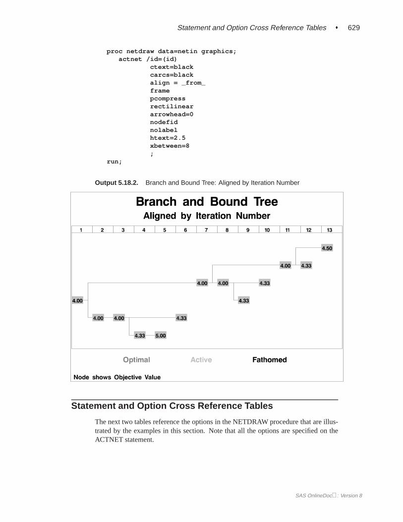
BOXWIDTH= options are reversed and so are the definitions of the XBETWEEN=and YBETWEEN= options. See Example 5.18 for an illustration of this option.

SEPARATEARCSseparates the arcs to follow distinct tracks. By default, the procedure draws all seg-ments of the arcs along a central track between the nodes, which may cause severalarcs to be drawn on top of one another. If the SEPARATEARCS option is speci-fied, the procedure may increase the values of the XBETWEEN= and YBETWEEN=options to accomodate the required number of lines between the nodes.

VMARGIN=integerspecifies the width of a vertical margin (in number of character cell positions) for thenetwork. The default width is 1.

VPAGES=vNYPAGES=v

specifies that the network diagram is to be produced usingv vertical pages. This,however, may not be possible due to intrinsic constraints on the output. For example,PROC NETDRAW requires that every vertical page should contain at least one y-level. Thus, the number of vertical pages can never exceed the number of horizontallevels in the network. The exact number of vertical pages used by the procedure isprovided in the–ORNETDR macro variable. See the “Macro Variable–ORNETDR”section on page 567 for further details.

The appearance of the diagram with respect to the VPAGES= option is also influ-enced by the presence of other related procedure options. The VPAGES= option per-forms the task of determining the number of horizontal pages in the absence of theHPAGES= option (or the NXNODES= option). If the COMPRESS or PCOMPRESSoption is specified (without the HPAGES= or NXNODES= options), the chart usesone horizontal page. If neither the COMPRESS nor PCOMPRESS option is speci-fied, the number of horizontal pages is computed in order to display as much of thechart as possible in a proportional manner.

WEB=variableHTML=variable

specifies the character variable in the Network data set which identifies a HTMLpage for each activity. The procedure generates an HTML image map using thisinformation for each node in the network diagram.

ZONEPATindicates that if a PATTERN= variable is not specified or is missing and if a ZONE=variable is present, then the node patterns are based on the value of the ZONE=variable.

Line-Printer OptionsBRKCHAR= brkchar

specifies the character used for drawing the zigzag break lines down the chart at breakpoints of the time axis. The default value is>. This option is valid only for time-scaled network diagrams.



FORMCHAR [ index list ]=‘string’specifies the characters used for node outlines and arcs. The value is a string 20characters long. The first 11 characters define the 2 bar characters, vertical and hor-izontal, and the 9 corner characters: upper-left, upper-middle, upper-right, middle-left, middle-middle (cross), middle-right, lower-left, lower-middle, and lower-right.These characters are used to outline each node and connect the arcs. The nineteenthcharacter denotes a right arrow. The default value of the FORMCHAR= option is|----|+|---+=|-/\<>* . Any character or hexadecimal string can be substi-tuted to customize the appearance of the diagram. Use an index list to specify whichdefault form character each supplied character replaces, or replace the entire defaultstring by specifying the full character replacement string without an index list. Forexample, change the four corners of each node and all turning points of the arcs toasterisks by specifying

FORMCHAR(3 5 7 9 11)= ’*****’

Specifying

formchar=’ ’ (11 blanks)

produces a network diagram with no outlines for the nodes (as well as no arcs).For further details about the FORMCHAR= option see Chapter 3, “The DTREEProcedure,” and Chapter 4, “The GANTT Procedure.”

REFCHAR=refcharspecifies the reference character used for drawing reference lines. The default valueis "|". This option is valid only for time-scaled network diagrams.

Details

Network Input Data Set

The Network input data set contains the precedence information, namely, theactivity-successor information for all the nodes in the network. The minimum amountof information that is required by PROC NETDRAW is the activity-successor infor-mation for the network. Additional information in the input data set can be used bythe procedure to add detail to the nodes in the diagram, or control the layout of thenetwork diagram.

There are three types of data sets that are typically used as the Network data set inputto PROC NETDRAW. Which type of data set you use depends on the stage of theproject:

� The Activity data set that is input to PROC CPM is the first type. In the initialstages of project definition, it may be useful to get a graphical representationof the project showing all the activity precedence constraints.

� The Schedule data set produced by PROC CPM (as the OUT= data set) is thesecond type. When a project is in progress, you may want to obtain a network


Network Input Data Set � 549

diagram showing all the relevant start and finish dates for the activities in theproject, in addition to the precedence constraints. You may also want to drawa time based network diagram, with the activities arranged according to thestart or finish times corresponding to any of the different schedules producedby PROC CPM.

� The Layout data set produced by PROC NETDRAW (as the OUT= data set) isthe third type. Often, you may want to draw network diagrams of the projectevery week showing updated information (as the project progresses); if thenetwork logic has not changed, it is not necessary to determine the placementof the nodes and the routing of the arcs every time. You can use the Layoutdata set produced by PROC NETDRAW that contains the node and arc posi-tions, update the start and finish times of the activities or merge in additionalinformation about each activity, and use the modified data set as the Networkdata set input to PROC NETDRAW. The new network diagram will have thesame layout as the earlier diagram but will contain updated information aboutthe schedule. Such a data set may also be useful if you want to modify thelayout of the network by changing the positions of some of the nodes. Seethe “Controlling the Layout” section on page 556 for details on how the lay-out information is used by PROC NETDRAW. If the Layout data set is used,it contains the variables–FROM– and –TO–; hence, it is not necessary tospecify the ACTIVITY= and SUCCESSOR= options. See Example 5.13 andExample 5.14 for illustrations of the use of the Layout data set.

The minimum information required by PROC NETDRAW from the Network dataset is the variable identifying each node in the network and the variable (or variables)identifying the immediate successors of each node. In addition, the procedure can useother optional variables in the data set to enhance the network diagram. The proce-dure uses the variables specified in the ID= option to label each node. The procedurealso looks for default variable names in the Network data set that are also addedto the list of ID variables; the default variable names are E–START, E–FINISH,L–START, L–FINISH, S–START, S–FINISH, A–START, A–FINISH, T–FLOAT,and F–FLOAT. The format used for determining the location of these variables withineach node is described in the “Format of the Display” section on page 553. See the“Variables in the Network Data Set” section on page 550 for a table of all the variablesin the Network data set and their interpretations by PROC NETDRAW.

If the Network data set contains the variables–X– and–Y– identifying the X and Ycoordinates of each node and each turning point of each arc in the network, then thisinformation is used by the procedure to draw the network. Otherwise, the precedencerelationships among the activities are used to determine the layout of the network.It is possible to specify only the node positions and let the procedure determine therouting of all the arcs. However, partial information cannot be augmented by theprocedure.

Note: If arc information is provided, the procedure assumes that it is complete andcorrect and uses it exactly as specified.



Variables in the Network Data Set

The NETDRAW procedure expects all the network information to be contained inthe Network input data set named by the DATA= option. The network information iscontained in the ACTIVITY and SUCCESSOR variables. In addition, the procedureuses default variable names in the Network data set for specific purposes. For exam-ple, the (–X–,–Y–) variables, if they are present in the Network data set, representthe coordinates of the nodes, the–SEQ– variable indexes the turning points of eacharc of the network, and so on.

In addition to the network precedence information, the Network data set may alsocontain other variables that can be used to change the default layout of the network.For example, the nodes of the network can be aligned in the horizontal directionusing the ALIGN= specification, or they can be divided into horizontal bands (orzones) using a ZONE variable.

Table 5.15 lists all of the variables associated with the Network data set and theirinterpretations by the NETDRAW procedure. Note that all the variables are identifiedto the procedure in the ACTNET statement. Some of the variables use default namesthat are recognized by the procedure to denote specific information, as explainedpreviously. The table indicates if the variable is default or needs to be identified inthe ACTNET statement.


Layout of the Network � 551

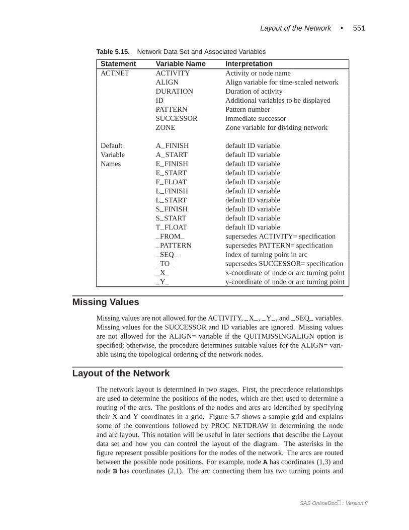
Table 5.15. Network Data Set and Associated Variables

Statement Variable Name InterpretationACTNET ACTIVITY Activity or node name

ALIGN Align variable for time-scaled networkDURATION Duration of activityID Additional variables to be displayedPATTERN Pattern numberSUCCESSOR Immediate successorZONE Zone variable for dividing network

Default A–FINISH default ID variableVariable A–START default ID variableNames E–FINISH default ID variable

E–START default ID variableF–FLOAT default ID variableL–FINISH default ID variableL–START default ID variableS–FINISH default ID variableS–START default ID variableT–FLOAT default ID variable

–FROM– supersedes ACTIVITY= specification

–PATTERN supersedes PATTERN= specification

–SEQ– index of turning point in arc

–TO– supersedes SUCCESSOR= specification

–X– x-coordinate of node or arc turning point

–Y– y-coordinate of node or arc turning point

Missing Values

Missing values are not allowed for the ACTIVITY,–X–, –Y–, and–SEQ– variables.Missing values for the SUCCESSOR and ID variables are ignored. Missing valuesare not allowed for the ALIGN= variable if the QUITMISSINGALIGN option isspecified; otherwise, the procedure determines suitable values for the ALIGN= vari-able using the topological ordering of the network nodes.

Layout of the Network

The network layout is determined in two stages. First, the precedence relationshipsare used to determine the positions of the nodes, which are then used to determine arouting of the arcs. The positions of the nodes and arcs are identified by specifyingtheir X and Y coordinates in a grid. Figure 5.7 shows a sample grid and explainssome of the conventions followed by PROC NETDRAW in determining the nodeand arc layout. This notation will be useful in later sections that describe the Layoutdata set and how you can control the layout of the diagram. The asterisks in thefigure represent possible positions for the nodes of the network. The arcs are routedbetween the possible node positions. For example, nodeA has coordinates (1,3) andnodeB has coordinates (2,1). The arc connecting them has two turning points and



is completely determined by the two pairs of coordinates (1.5, 3) and (1.5, 1) ; here,X=1.5 implies that the position is midway between the X coordinates 1 and 2.

Figure 5.7. Sample Grid and Coordinates for Node and Arc Layout

PROC NETDRAW sets X=1 for all nodes with no predecessors; the X coordinates forthe other nodes are determined so that each node is placed to the immediate right ofall its predecessors; in other words, no node will appear to the left of any of its prede-cessors or to the right of any of its successors in the network diagram. The nodes areplaced in topological order: a node is placed only after all its predecessors have beenplaced. Thus, the node-placement algorithm requires that there should be no cycles inthe network. The Y coordinates of the nodes are determined by the procedure usingseveral heuristics designed to produce a reasonable compact diagram of the network.To draw a network that has cycles, use the BREAKCYCLE option, or you can spec-ify the node coordinates or an ALIGN= variable to circumvent the requirement of atopological ordering of the nodes (see the second part of Example 5.12.

Note that the X and Y coordinates fix only a relative positioning of the nodes andarcs. The actual distance between two nodes, the width and height of each node, andso on can be controlled by specifying desired values for the options that control theformat of the display, namely, BOXHT=, BOXWIDTH=, and so on. See the “Formatof the Display” section on page 553 for details on these options.

By default, the procedure routes the arcs using a simple heuristic that uses, at most,four turning points: the arc leaves the predecessor node from its right edge, turns up ordown according to whether the successor is above or below the current node position,then tracks horizontally across to the verticalcorridor just before the successor node,


Format of the Display � 553

and then tracks in a vertical direction to meet the successor node. For example, seethe tracking of the arc connecting nodesCandD in Figure 5.7.

For networks that include some nonstandard precedence constraints, the arcs may bedrawn from and to the appropriate edges of the nodes, depending on the type of theconstraint.

The default routing of the arcs may lead to an unbalanced diagram with too manyarcs in one section and too few in another. The DP option in the ACTNET statementcauses the procedure to use a dynamic programming algorithm to route the arcs. Thisalgorithm tries to route the arcs between the nodes so that not too many arcs passthrough any interval between two nodes. The procedure sets the maximum numberof arcs that are allowed to be routed along anycorridor to be equal to the maximumnumber of successors for any node. The HTRACKS= and VTRACKS= options en-able you to set these maximum values: HTRACKS specifies the maximum number ofarcs that are allowed to pass horizontally through any point while VTRACKS speci-fies the same for arcs in the vertical direction. See Example 5.7 for an illustration ofthe HTRACKS= option.

The layout of the network for time-scaled and zoned network diagrams is discussed inthe “Time-Scaled Network Diagrams” section on page 558 and the “Zoned NetworkDiagrams” section on page 560, respectively. The “Organizational Charts or TreeDiagrams” section on page 561 describes the layout of the diagram when the TREEoption is specified.

Format of the Display

As explained in the previous section, the layout of the network is determined by theprocedure in terms of X and Y coordinates on a grid as shown in Figure 5.7. Thedistance between nodes and the width and height of each node is determined by thevalues of the format control options: XBETWEEN=, YBETWEEN=, BOXHT=, andBOXWIDTH= . Note that, if the ROTATETEXT option is specified (in graphicsmode), then the definitions of the BOXHT= and BOXWIDTH= options are reversedand so are the definitions of the XBETWEEN= and YBETWEEN= options.

The amount of information that is displayed within each node is determined by thevariables specified via the ID= option, the number of default variables found in theNetwork data set, and whether the NOLABEL and NODEFID options are speci-fied. The values of the variables specified via the ID= option are placed within eachnode on separate lines. If the NOLABEL option is in effect, only the values of thevariables are written; otherwise, each value is preceded by the name of the ID vari-able truncated to three characters. Recall from the “Syntax” section on page 530that, in addition to the variables specified using the ID= option, the procedure alsodisplays additional variables. These variables are displayed below the variables ex-plicitly specified via the ID= option, in pre-determined relative positions within eachnode (see Figure 5.8.)



ID1...IDnActivity variable DurationvariableE–START E–FINISHL–START L–FINISHS–START S–FINISHA–START A–FINISHT–FLOAT F–FLOAT

Figure 5.8. Display Format for the Variables within Each Node

Note: If a node is identified as a successor (via a SUCCESSOR variable) and is neveridentified via the ACTIVITY variable, the ID values for this node are never definedin any observation; hence, this node will have missing values for all the ID variables.

If the SHOWSTATUS option is specified and the Network data set contains progressinformation (in either the STATUS variable or the A–START and A–FINISH vari-ables), the procedure appropriately marks each node referring to activities that arecompleted or in progress. See Example 5.8 for an example illustrating the SHOW-STATUS option.

The features just described pertain to all three modes of the procedure. In addition,there are options to control the format of the display that are specific to the mode ofinvocation of the procedure. For graphics quality network diagrams, you can choosethe color and pattern used for each node separately by specifying a different patternnumber for the PATTERN= variable, identified in the ACTNET statement (for de-tails, see the “Graphics Version” section on page 565). For line-printer or full-screennetwork diagrams, the FORMCHAR= option enables you to specify special boxingcharacters that enhance the display; for full-screen network diagrams, you can alsochoose the color of the nodes using the PATTERN= option.

By default, all arcs are drawn along the center track between two consecutive nodes.The SEPARATEARCS option, which is available in the graphics version, separatesarcs in the same corridor by drawing them along separate tracks, thus preventing themfrom being drawn on top of each other.

If the network fits on one page, it is centered on the page; in the graphics mode, youcan use the NOVCENTER option to prevent centering in the vertical direction so thatthe network is drawn immediately below the title. If the network cannot fit on onepage, it is split onto different pages appropriately. See the “Page Format” section onpage 555 for a description of how the pages are split.


Layout Data Set � 555

Page Format

7 8 9

4 5 6

1 2 3

Figure 5.9. Page Layout

As explained in the “Format of the Display” section on page 553, if the network fitson one page, it is centered on the page (unless the NOVCENTER option is speci-fied); otherwise, it is split onto different pages appropriately, and each page is drawnstarting at the bottom left corner. If the network is drawn on multiple pages, the pro-cedure numbers each page of the diagram on the top right corner of the page. Thepages are numbered starting with the bottom left corner of the entire picture. Thus, ifthe network diagram is broken into three horizontal and three vertical levels and youwant to paste all the pieces together to form one picture, they should be arranged asshown in Figure 5.9.

The number of pages of graphical output produced by the NETDRAW proceduredepends on several options such as the NXNODES=, NYNODES=, HPAGES=,VPAGES=, COMPRESS, PCOMPRESS, HTEXT=, and the ID= options. The valueof the HTEXT= option and the number of variables specified in the ID= options deter-mines the size of each node in the network diagram, which in turn affects the numberof horizontal and vertical pages needed to draw the entire network. The number ofpages is also affected by the global specification of the HPOS=, VPOS=, HSIZE=,and VSIZE= graphics options.

The COMPRESS and PCOMPRESS options force the entire network diagram to bedrawn on a single page. You can explicitly control the number of horizontal andvertical pages using the HPAGES= and VPAGES= options. The NXNODES= andNYNODES= options enable you to specify the number of nodes in the horizontaland vertical directions, respectively, on each page of the network diagram.

For examples of these options and how they affect the network diagram output, seeExample 5.5.

Layout Data Set

The Layout data set produced by PROC NETDRAW contains all the informationneeded to redraw the network diagram for the given network data. In other words,the Layout data set contains the precedence information, the ID variables that are used



in the current invocation of the procedure, and variables that contain the coordinateinformation for all the nodes and arcs in the network.

The precedence information used by the procedure is defined by two new variablesnamed–FROM– and –TO– , which replicate the ACTIVITY and SUCCESSORvariables from the Network data set. Note that the Layout data set has only one–TO–variable even if the Network data set has multiple SUCCESSOR variables; if a givenobservation in the Network data set defines multiple successors for a given activity,the Layout data set defines a new observation for each of the successors. In fact, foreach (node, successor) pair, a sequence of observations, defining the turning pointsof the arc, is saved in the Layout data set; the number of observations correspondingto each pair is equal to one plus the number of turns in the arc connecting the node toits successor. Suppose that a node ‘C’ has two successors, ‘D’ and ‘E’, and the arcsconnecting ‘C’ and ‘D’ and ‘C’ and ‘E’ are routed as per Figure 5.7. Then, Figure5.10 illustrates the format of the observations corresponding to the two (–FROM– ,

–TO–) pairs of nodes, (‘C’, ‘D’) and (‘C’, ‘E’).

–FROM– –TO– –X– –Y– –SEQ– –PATTERN ID variables

C D 3 1 0 1C D 3.5 1 1 .C D 3.5 2.5 2 .C D 5.5 2.5 3 .C D 5.5 3 4 .C E 3 1 0 1

. .

. .

. .

Figure 5.10. Sample Observations in the Layout Data Set

For every (node, successor) pair, the first observation (–SEQ– = ‘0’) gives the coor-dinates of the predecessor node; the succeeding observations contain the coordinatesof the turning points of the arc connecting the predecessor node to the successor.The data set also contains a variable called–PATTERN, which contains the patternnumber that is used for coloring the node identified by the–FROM– variable. Thisvariable is missing for observations with–SEQ– > 0.

Controlling the Layout

As explained in the “Layout of the Network” section on page 551 section, the pro-cedure uses the precedence constraints between the activities to draw a reasonablediagram of the network. A very desirable feature in any procedure of this nature isthe ability to change the default layout. PROC NETDRAW provides two ways ofmodifying the network diagram:

� via the full-screen interface


Time-Scaled Network Diagrams � 557

� via the Network data set

The full-screen method is useful for manipulating the layout of small networks, es-pecially networks that fit on a handful of screens. You can use the full-screen modeto examine the default layout of the network and move the nodes to desired locationsusing the MOVE command from the command line or by using the appropriate func-tion key. When a node is moved, the procedure reroutes all the arcs that connect toor from the node; other arcs are unchanged. For details about the MOVE command,see the “Full-screen Version” section on page 562.

You can use the Network data set to modify or specify completely the layout of thenetwork. This method is useful if you want to draw the network using informationabout the network layout that has been saved from an earlier invocation of the proce-dure. Sometimes you may want to specify only the positions of the node and let theprocedure determine the routing of the arcs. The procedure looks for three defaultvariables in the data set:–X– , –Y– , and–SEQ– . The–X– and–Y– variables areassumed to denote the X and Y coordinates of the nodes and all the turning points ofthe arcs connecting the nodes. The variable–SEQ– is assumed to denote the orderof the turning points. This interpretation is consistent with the values assigned to the

–X– , –Y– , and–SEQ– variables in the Layout data set produced by PROC NET-DRAW. If there is no variable called–SEQ– in the data set, the procedure assumesthat only the node positions are specified and uses the specified coordinates to placethe nodes and determines the routing of the arcs corresponding to these positions.If there is a variable called–SEQ– , the procedure requires that the turning pointsfor each arc be specified in the proper order, with the variable–SEQ– containingnumbers sequentially starting with 1 and continuing onward. The procedure thendraws the arcs exactly as specified, without checking for consistency or interpolatingor extrapolating turning points that may be missing.

The ALIGN= variable provides another means of controlling the node layout (see the“Time-Scaled Network Diagrams” section on page 558). This variable can be used tospecify the X coordinates for the different nodes of the network; the procedure thendetermines the Y coordinates. Note that time-scaled network diagrams (without anALIGN= specification) are equivalent to network diagrams drawn with the ALIGN=variable being set to the E–START variable.

You can also control the placement of the nodes using the ZONE= option (see the“Zoned Network Diagrams” section on page 560). The procedure uses the valuesof the ZONE variable to divide the network into horizontal zones. Thus, you cancontrol the horizontal placement of the nodes via the ALIGN= option and the verticalplacement of the nodes via the ZONE= option.

For networks that have a tree structure, the TREE option draws the network as atree, thus providing another layout option (see the “Organizational Charts or TreeDiagrams” section on page 561). The procedure draws the tree from left to right,with the root at the left edge of the diagram. Thus, the children of each node aredrawn to the right of the node. In the graphics mode of invocation, you can use theROTATETEXT option in conjunction with the global graphics option ROTATE toobtain a top-down tree diagram.



Time-Scaled Network Diagrams

By default, PROC NETDRAW uses the topological ordering of the activity networkto determine the X coordinates of the nodes. As a project progresses, you may wantto display the activities arranged according to their time of occurrence. Using theTIMESCALE option, you can draw the network with a time axis at the top andthe nodes aligned according to their early start times, by default. You can use theALIGN= option to specify any of the other start or finish times in the Network dataset. In fact, PROC NETDRAW enables you to align the nodes according to any nu-meric variable in the data set.

If the TIMESCALE option is specified without any ALIGN= specification, the pro-cedure chooses one of the following variables as the ALIGN= variable: E–START,L–START, S–START, or A–START, in that order. The first of these variables that isfound is used to align the nodes. The minimum and maximum values of the ALIGN=variable are used to determine the time axis. The format of this variable is used todetermine the default value for the MININTERVAL= option. The value of the MIN-INTERVAL= option (or the default value) is used to determine the format of the timeaxis. You can override the format based onmininterval by specifying the desired for-mat for the ALIGN= variable (using the FORMAT statement to indicate a standardSAS format or a special user-defined format) and the USEFORMAT option in theACTNET statement. Table 5.16 lists the valid values ofmininterval corresponding tothe type of the ALIGN= variable and the default format corresponding to each valueof mininterval. For each value in the first column, the first value ofmininterval listedis the default value of the MININTERVAL= option corresponding to that type of theALIGN= variable.

Several options are available in PROC NETDRAW to control the spacing of the nodesand the scaling of a time-scaled network diagram:

� The MININTERVAL= option enables you to scale the network diagram: onetick mark is associated with one unit ofmininterval. Thus, if mininterval isDAY, each column is used to represent one day and all activities that start onthe same day are placed in the same column. By default, the procedure omitsany column (tick mark) that does not contain any node.

� The LINEAR option enables you to print a tick mark corresponding to everyday (or the unit ofmininterval). Note that, for a project that has few activitiesspread over a large period of time, the LINEAR option can lead to a networkdiagram that is very wide.

� The MAXNULLCOLUMN= option specifies the maximum number of emptycolumns that is allowed between two consecutive nonempty columns. TheLINEAR option is equivalent to specifyingmaxncol = infinity, while the defaulttime-scaled network diagram is drawn withmaxncol = 0.

� The NLEVELSPERCOLUMN= option enables you to contract the networkdiagram by combining a few columns. For example, ifmininterval is DAY andnlevelspercol is 7, each column contains activities that start within seven daysof each other; note that the same effect can be achieved by settingminintervalto be WEEK.


Time-Scaled Network Diagrams � 559

Table 5.16. MININTERVAL Values and Axis Format

ALIGN Variable Type MININTERVAL Axis Label Formatnumber numeric formatSAS time HOUR HHMM5.

MINUTE HHMM5.SECOND TIME8.

SAS date DAY DATE7.WEEKDAY DATE7.WEEK DATE7.MONTH MONYY5.QTR MONYY5.YEAR MONYY5.

SAS datetime DTDAY DATE7.WORKDAY DATE7.DTWRKDAY DATE7.DTSECOND DATETIME16.DTMINUTE DATETIME16.DTHOUR DATETIME13.

DTWEEK DATE7.DTMONTH MONYY5.DTQTR MONYY5.DTYEAR MONYY5.

The node-placement algorithm described in the “Layout of the Network” section onpage 551 is modified slightly for time-scaled network diagrams. The X coordinate ofeach node is determined by the value of the ALIGN= variable. The scaling optionsjust described are used to determine the tick mark corresponding to the node. The Ycoordinate is determined as before. Once the node placement is completed, the arcrouting algorithm is the same as described earlier.

Note: Since the node placement for time-scaled networks is determined by theALIGN= variable, it is possible that some of the arcs between the nodes may have tobe routed from right to left instead of from left to right; in other words, there may besome backward arcs. Note also that, if the ALIGN= variable is used to determine theX coordinates of the nodes, the procedure can also draw networks that contain cycles(see the second part of Example 5.12).

Several other options are available to control the appearance of time-scaled networkdiagrams: AUTOREF, BRKCHAR=, CAXIS=, CREF=, CREFBRK=, FRAME,LREF=, LREFBRK=, NOREPEATAXIS, NOTIMEAXIS, REFBREAK, RE-FCHAR=, and SHOWBREAK. These options are described in the “Syntax” sectionon page 530.



Zoned Network Diagrams

Most projects have at least one natural classification of the different activities in theproject: department, type of work involved, location of the activity, and so on. TheZONE= option enables you to divide the network diagram into horizontal bands orzones corresponding to this classification. The procedure uses the following rules toplace the nodes in a zoned network diagram:

� The values of the ZONE variable are used to define as many zones as there aredistinct values of this variable.

� Each node of the network is drawn within its corresponding zone.

� The number of rows within each zone is determined by the maximum numberof nodes in any given column that correspond to that zone.

� The values of the ZONE variable do not need to be sorted in any particularorder, nor do they need to be grouped by distinct values.

� The zones are ordered according to the order of appearance of the differentvalues of the ZONE variable in the Network data set. This enables you tochoose any order for the zone values.

� For arcs that connect two nodes within the same zone, the arc lies entirelywithin the zone; in other words, all the turning points of the arc have Y co-ordinates that are between the minimum and maximum Y coordinates for thezone.

� Each zone is labeled by the value of the ZONE variable unless the NO-ZONELABEL option is specified.

� Each zone is separated from the next by a horizontal line drawn across thewidth of the network unless the NOZONELABEL option is specified.

� In the graphics and full-screen modes of invocation of the procedure, you canuse the ZONEPAT option to color the nodes in each zone differently usingdifferent pattern statements. In the graphics mode, the first zone uses the firstPATTERN statement, the second zone uses the second PATTERN statement,and so on; in full-screen mode, the colors available for the device are repeatedin cyclic order. Note that the values of the PATTERN= variable (or the default

–PATTERN variable, if it exists in the Network data set) override the nodepatterns dictated by the ZONEPAT option.


Full-screen Version � 561

Organizational Charts or Tree Diagrams

The NETDRAW procedure automatically draws any acyclic network. They do nothave to be representations of a project. You can also use the procedure to draw ageneral directed graph that has cycles, if node location is specified or if the BREAK-CYCLE option is specified. The procedure attempts to draw the network in a compactfashion, which may not always produce the expected result. Trees form one such classof directed graphs that have an inherent natural layout that may not be produced bythe default layout of PROC NETDRAW. The TREE option in the ACTNET statementexploits the tree structure of the network by laying the nodes out in the form of a tree.

A directed graph is said to be a tree if it has a root and there is a unique directed pathfrom the root to every node in the tree. An equivalent characterization of a tree isthat the root node has no predecessors and every other node has exactly one prede-cessor (Even 1979). Typical examples of trees that arise in project management areorganizational charts or work breakdown structures. If the TREE option is specified,the NETDRAW procedure checks if the network has a tree structure and draws thenetwork with the root at the left edge of the diagram and the children of each nodeappearing to the right of the node. In other words, the tree is drawn from left to right.

The NETDRAW procedure enables you to specify multiple trees in the same Networkdata set; each tree is drawn separately in the same diagram with all the roots appearingat the left edge of the diagram. Thus, you can use the TREE option as long as everynode in the network hasat mostone predecessor. It you specify the TREE option andsome node has multiple predecessors, the TREE option is ignored and the procedureuses the default node-layout algorithm.

There are several features that control the appearance of the tree:

� The children of each node are placed in the order of occurrence in the Net-work data set. The (–X–,–Y–) coordinates of each node are required to beintegers. The procedure attempts to place each node at the center of all itschildren, subject to the requirement that the coordinates must be integers. Thisrequirement may cause some of the nodes to be positioned slightly off-center.See Example 5.15.

� The SEPARATESONS option separates the children of a node, if necessary, toenable the parent node to be exactly centered with respect to its children. Seethe second part of Example 5.15.

� The CENTERSUBTREE option can be used to center each node with respect tothe entire subtree originating from the node instead of centering it with respectto its children.

� In graphics mode, you can change the orientation of the network to be fromtop to bottom instead of from left to right. To do so, use the ROTATETEXToption in the ACTNET statement to rotate the text within the nodes and theROTATE global graphics option to rotate the entire diagram by 90 degrees.See Example 5.18 for an illustration of this feature.



Full-screen Version

You can invoke PROC NETDRAW in full-screen mode by specifying FS (orFULLSCREEN) in the PROC NETDRAW statement. The statement specificationsare the same as for the line-printer mode. The full-screen mode offers you a con-venient way to browse the network diagram of the project and change the layout ofthe network by moving the nodes of the network to desired locations. However, youcannot move a node to any position that violates the precedence constraints that mustbe satisfied by the node. In other words, you cannot move a node to the left of anyof its predecessors or to the right of any of its successors. For time-scaled networkdiagrams, you cannot move a node out of the column corresponding to the value ofthe ALIGN= variable. For zoned network diagrams you cannot move a node out ofits zone.

The format control options are treated in the same way as for the line-printer version,with some minor changes. It is assumed that the main purpose of invoking the proce-dure is to gain a general picture of the layout of the entire network and to modify itto some extent. In an effort to display as much of the network as possible, the initialdisplay on the screen is drawn with only one row and three columns for each node.In other words, the BOXHT=, BOXWIDTH=, XBETWEEN=, and YBETWEEN=options are ignored by the procedure in drawing the initial display. However, the full-screen commands supported by PROC NETDRAW enable you to change the scale ofthe diagram. You can display as much or as little information within each node by in-voking the SCALE ROW or the SCALE COL command or both. The SCALE MAXcommand causes the procedure to display the diagram using the values specified inthe ACTNET statement or the dimensions that would be required to display all the IDinformation, whichever is larger. The SCALE RESET command returns the scalingto the initial values used for display.

The nodes of the network are color coded on the basis of the PATTERN variable. Ifthere is no PATTERN variable, then the nodes are color coded depending on whetherthe activities are normal, critical, or supercritical. The nodes are drawn in reversevideo. By default, the nodes are drawn without an outline; however, there is anOUTLINE command that lets you toggle back and forth between an outlined or non-outlined node. Using an outline for the node is useful if you want to obtain a printoutof the screen display using SPRINT; it helps mark the boundary of each node clearly.

CommandsTable 5.17 lists the commands that can be invoked from the command line in thefull-screen version of PROC NETDRAW. These commands are explained in greaterdetail in this section.


Full-screen Version � 563

Table 5.17. Full-Screen Commands and Their Purposes

Controlling Changing NetworkScrolling Display Layout ExitingBACKWARD OUTLINE CLEAR GENDFORWARD SCALE MOVE ENDLEFT CANCELRIGHTTOPBOTTOMVSCROLLHSCROLL

BACKWARDscrolls towards the top of the network by the VSCROLL amount. BACKWARDMAX scrolls to the top of the network. You can specify the vertical scroll amount forthe current command as BACKWARD PAGE| HALF| n.

BOTTOMscrolls to the bottom of the network.

CANCELends the current invocation of the procedure.

CLEARclears any outstanding move commands.

GENDends the current invocation of the procedure after drawing the network in graphicsmode with the compress option.

ENDends the current invocation of the procedure.

FORWARDscrolls toward the bottom of the network by the VSCROLL amount. FORWARDMAX scrolls to the bottom of the network. You can also specify the vertical scrollamount for the current command as FORWARD PAGE| HALF| n.

HELPdisplays a help screen listing all the full-screen commands specific to PROC NET-DRAW.

HOMEmoves the cursor to the command line.

HSCROLLsets the amount that information scrolls horizontally when you execute the LEFT orRIGHT command. The format is HSCROLL PAGE| HALF| n. The specificationis assumed to be in number of horizontal levels. HSCROLL PAGE sets the scrollamount to be the number of horizontal levels that fit on one screen; HSCROLL HALFis half that amount; HSCROLLn sets the horizontal scroll amount ton levels.



KEYSdisplays current function key settings for the NETDRAW procedure.

LEFTscrolls toward the left boundary of the network by the HSCROLL amount. LEFTMAX scrolls to the left boundary. You can specify the horizontal scroll amount forthe current command as LEFT PAGE| HALF| n.

MOVEspecifies a node to be moved or a place to move a node to. You can specify these inany order. Thus, you can first position the cursor on the node that you want to move,issue the MOVE command, and then position the cursor at a target position and issuethe MOVE command again. If the target position is valid, the node is moved. You canalso first specify the target position and then indicate the node that is to be moved.

Note: For a standard network, a node cannot be moved to any position that violatesthe topological ordering of the nodes in the network. For time-scaled network dia-grams, you cannot move a node to a level corresponding to a different tick mark. Forzoned network diagrams, you cannot move a node out of its zone.

OUTLINEcauses an outline to be drawn around each node in the network. This is useful if youwant to print a copy of the screen by using the SPRINT command. The OUTLINEcommand works like an on/off switch: you can turn it off by entering the commandagain.

RIGHTscrolls toward the right boundary of the network by the HSCROLL amount. RIGHTMAX scrolls to the right boundary. You can also specify the horizontal scroll amountfor the current command as RIGHT PAGE| HALF| n.

SCALEcontrols the scaling of the nodes and the space between nodes. The format ofthis command is SCALE MAX| MIN | RESET| ROW MAX| COL MAX | ROWMIN | COL MIN| ROW n | COL n| +n| �n. The numbern denotes the number ofcharacter positions. SCALE MIN displays as many nodes on the screen as can fit.SCALE MAX allows as many rows and columns per node as is required to displayall the information that pertains to it. SCALE ROW MAX displays the maximumnumber of rows per node. SCALE COL MAX displays the maximum number ofcolumns per node. SCALE ROWn sets the number of rows per node ton. SCALEROW+n increases the number of rows per node byn. SCALE COLn sets the num-ber of columns per node ton. SCALE COL+n increases the number of columns pernode byn. SCALE RESET sets the values to be the same as for the initial display.Note that none of these values can be greater than the dimensions of the screen.

TOPscrolls to the top of the network.

VSCROLLsets the amount by which information scrolls vertically when you execute the BACK-WARD or FORWARD command. The format is VSCROLL PAGE| HALF| n. The


Graphics Version � 565

specification is assumed to be in number of vertical levels. VSCROLL PAGE sets thescroll amount to be the number of vertical levels that fit on one screen; VSCROLLHALF is half that amount; VSCROLLn sets the vertical scroll amount ton levels.

Full-Screen Global CommandsMost of the global commands used in SAS/FSP software are also valid with PROCNETDRAW. Some of the commands used for printing screens are described in the“Global Commands” section of Chapter 4, “The GANTT Procedure.”

Graphics Version

Several options are available in the ACTNET statement to enhance the appearanceof the network diagram in graphics mode. These are described in the “GraphicsOptions” section on page 542. The format control options BOXWIDTH=, BOXHT=,XBETWEEN=, and YBETWEEN= are also valid in this mode and can be used tocontrol the width and height of each node and the distance between the nodes. Theseparameters are specified in terms of number of character cell positions. The numberof positions available on one page depends on the graphics device that is used; thus,if a plotter is used with large paper, more of the network will be drawn on a singlepage. Further, you can control the number of character cell positions on a page bychanging the values of the global graphics options (HPOS= and VPOS=).

You can also control the number of nodes on a given page by specifying the NXN-ODES= and NYNODES= options. The HPAGES= and VPAGES= options controlthe number of pages in the horizontal and vertical directions. Thus, you have a widedegree of control over the amount of information displayed on each page of the net-work diagram.

Another option that is available in graphics mode to control the appearance of yournetwork diagrams is the specification of a PATTERN variable in the ACTNET state-ment. If the variable is named–PATTERN, you do not need to use the PATTERN=option; the procedure looks for such a variable by default. You can use this variableto specify the PATTERN definition that is to be used for filling each node of the net-work. Note that if the value of the–PATTERN variable isj for a particular node,PROC NETDRAW uses the specifications in thejth generatedPATTERNdefinition,not the specifications in the PATTERNj statement.

The patterns that can be used with PROC NETDRAW are any of the patterns that canbe used for drawing bars (not ones that are used for drawing maps). However, for thetext to be visible, you may want to restrict the patterns used to be empty and changeonly the color of the pattern. You can also use solid fills with a light color and specifythe COUTLINE= and CCRITOUT= options to mark noncritical and critical nodeswith different colors for the outline.

SeeSAS/GRAPH Software: Referencefor details about creating, canceling, review-ing, and altering PATTERN definitions. For a brief description of the PATTERNstatement and for a list of available patterns, see Chapter 4, “The GANTT Procedure.”

If a PATTERN variable is not specified, the procedure uses the values of theE–FINISH and L–FINISH variables (if these variables exist in the Network dataset) to determine if activities in the project are normal, critical, or supercritical. The



procedure then uses the firstgeneratedPATTERN definition to fill the nodes cor-responding to noncritical activities, the secondgeneratedPATTERN definition fornodes corresponding to critical activities, and the thirdgeneratedPATTERNdefini-tion for nodes corresponding to supercritical activities.

For zoned network diagrams, if there is no PATTERN variable, the ZONEPAT optionenables you to color the nodes based on the values of the ZONE= variable.

Using the Annotate Facility

The Annotate facility enables you to enhance graphics output produced by PROCNETDRAW. To use this facility you must create an Annotate data set, which con-tains a set of graphics commands that can be superimposed on the network diagram.This data set has a specific format and must contain key variables as described inSAS/GRAPH Software: Reference, First Edition. That chapter lists the variables thatare required in this data set and explains the coordinate systems used by the Annotatefacility. The present section explains the use of data coordinates specifically withreference to the NETDRAW procedure.

When annotating a graph produced by any of the graphics procedures, it is helpfulto use data coordinates that refer to the data values corresponding to the graph thatis being annotated. For example, if you want to label a particular node of a networkdiagram with additional text, you can position the text accurately if you use data co-ordinates instead of screen coordinates. With respect to PROC NETDRAW, the An-notate facility uses the–X– and–Y– values in the Layout data set as the basis for thedata coordinate system. To use this feature, you can invoke PROC NETDRAW (withthe NODISPLAY option, if necessary) for the given network to produce the Layoutdata set that contains the–X– and–Y– coordinates for each node of the network.This data set can then be used to create the required Annotate data set containing thegraphics commands positioning the primitives appropriately on the diagram using thedata coordinates. See Example 5.16 and Example 5.17 for illustrations of this feature.

Note: The data coordinate system enables you to annotate the graph even if it spansmultiple pages. However, each annotation must be entirely contained within a givenpage. For example, you cannot annotate a line on the network diagram that runs fromone page of the diagram to another.

Web Enabled Network Diagrams

The WEB= variable enables you to define a HTML reference for each activity.This HTML reference is associated with the node corresponding to the activity.The WEB= variable is a character variable and the values need to be of the form"HREF=htmlpage".

In addition you can also store the coordinate and link information defined via theWEB= option in a SAS data set by specifying the IMAGEMAP= option in the PROCNETDRAW statement. By processing this SAS data set using a DATA step, you cangenerate customized HTML pages for your network diagram.


Computer Resource Requirements � 567

Macro Variable –ORNETDR

The NETDRAW procedure defines a macro variable named–ORNETDR. This vari-able contains a character string that indicates the status of the procedure. It is set atprocedure termination. The form of the–ORNETDR character string is STATUS=REASON= , where STATUS= is either SUCCESSFUL or ERROR–EXIT and REA-SON= (if PROC NETDRAW terminated unsuccessfully) can be one of the following:

CYCLE

BADDATA –ERROR

MEMORY–ERROR

IO–ERROR

SEMANTIC–ERROR

SYNTAX–ERROR

NETDRAW–BUG

UNKNOWN–ERROR

This information can be used when PROC NETDRAW is one step in a larger pro-gram that needs to determine whether the procedure terminated successfully or not.Because–ORNETDR is a standard SAS macro variable, it can be used in the waysthat all macro variables can be used.

In addition to the "STATUS= REASON= " string indicating the status of the pro-cedure, the macro variable–ORNETDR also provides some information about thenetwork diagram produced by the current invocation of PROC NETDRAW.

The information given in–ORNETDR is described below along with the keywordidentifying it. It should be noted that these values refer to those actually used inproducing the network diagram and are not necessarily the same as those specified inthe invocation of the procedure.

� HPAGES= The number of horizontal pages

� VPAGES= The number of vertical pages

� SEGNAME= The name of the first network diagram segment in graphics mode

Note: Some of the information may be redundant or predictable in certain displaymodes. For example, the value of the SEGNAME= option is empty in line-printerand full-screen modes. The values of the HPAGES= and VPAGES= options are equalto 1 in full-screen mode.



Computer Resource Requirements

There is no inherent limit on the size of the network that can be drawn with the NET-DRAW procedure. Naturally, there needs to be a sufficient amount of core memoryavailable in order to invoke and initialize the SAS system. Furthermore, the amountof memory required depends on the mode of invocation of the procedure. As far aspossible, the procedure attempts to store all the data in core memory. However, if theproblem is too large to fit in core memory, the procedure resorts to the use of utilitydata sets and swaps between core memory and utility data sets as necessary.

The storage requirement for the data area required by the procedure is proportionalto the number of nodes and arcs in the network. The memory required is further in-creased by the use of the DP option in the ACTNET statement. Recall that this optionrequests the use of a dynamic programming algorithm to route the arcs between thenodes, and such algorithms tend to grow exponentially with the size of the problembeing solved.

Examples

This section contains 18 examples that illustrate several features of the NETDRAWprocedure. Most of the examples use the data from the Widget Manufacturing Projectdescribed in Chapter 2, “The CPM Procedure.” Two tables, Table 5.18 and Table 5.19,at the end of this section list all the examples in this chapter and the options andstatements in the NETDRAW procedure that are illustrated by each example.

Example 5.1. Line-Printer Network Diagram

This example uses the data setWIDGET that was used in Example 2.2 in Chap-ter 2, “The CPM Procedure,” to illustrate the Activity-on-Node representation of theproject. The following program invokes PROC NETDRAW twice. First, the Activitydata setWIDGET is used as input to the procedure. The activity and successor in-formation is identified via the ACTIVITY= and SUCCESSOR= options in the ACT-NET statement. The LINEPRINTER option is specified, producing the line-printernetwork diagram shown in Output 5.1.1.

/* Activity-on-Node representation of the project */data widget;

input task $ 1-12 days succ1 $ 19-30succ2 $ 33-44succ3 $ 47-58;

datalines;Approve Plan 5 Drawings Anal. Market Write SpecsDrawings 10 PrototypeAnal. Market 5 Mkt. Strat.Write Specs 5 PrototypePrototype 15 Materials FacilityMkt. Strat. 10 Test Market MarketingMaterials 10 Init. Prod.Facility 10 Init. Prod.Init. Prod. 10 Test Market Marketing Evaluate


Example 5.1. Line-Printer Network Diagram � 569

Evaluate 10 ChangesTest Market 15 ChangesChanges 5 ProductionProduction 0Marketing 0;

title ’Widget Manufacture’;options ps=32 ls=78;proc netdraw data=widget lineprinter;

actnet / activity=task successor=(succ1 succ2 succ3);run;

Output 5.1.1. Line-Printer Network Diagram

Widget Manufacture

-------------- ---------------->|Drawings |--- -->|Materials |---| -------------- | | -------------- || | | || | | || | |------------------+--| | | || | | |

-------------- | -------------- | -------------- | -------------- ||Approve Plan|--+->|Write Specs |---->|Prototype |--+->|Facility |---->-------------- | -------------- -------------- | --------------

| || || || || || -------------- -------------- |-->|Anal. Market|---->|Mkt. Strat. |------------------------

-------------- --------------



Widget Manufacture

---------------->|Test Market |---| -------------- || || |

----------------| || || |

-------------- | -------------- | -------------- --------------|Init. Prod. |--+->|Evaluate |---->|Changes |---->|Production |-------------- | -------------- -------------- --------------

|||||| --------------

------------------>|Marketing |--------------

Next, PROC CPM is invoked to schedule the project, and the resulting Scheduledata set is used as input to the NETDRAW procedure. In addition to the ACTIV-ITY= and SUCCESSOR= options, the DURATION= option is used in the ACTNETstatement. The DURATION= option adds the values of the DURATION variablewithin each node of the network. The procedure also displays the values of theE–START, E–FINISH, L–START, L–FINISH, T–FLOAT, andF–FLOAT vari-ables within each node. The network is displayed in Output 5.1.2.

proc cpm data=widget out=scheddate=’2dec91’d;

activity task;successor succ1 succ2 succ3;duration days;run;

options ps=45 ls=90;title2 ’Schedule Information’;proc netdraw data=sched lineprinter;

actnet / activity=tasksuccessor=(succ1 succ2 succ3)duration = days;

run;


Example 5.1. Line-Printer Network Diagram � 571

Output 5.1.2. Project Schedule

Widget ManufactureSchedule Information

-------------------------|Drawings Dur:10|

-->|ES:07DEC91 EF:16DEC91|--- -->| |LS:07DEC91 LF:16DEC91| | || |TF: 0 FF: 0 | | || ------------------------- | || | || | || | |--| | || | |

------------------------- | ------------------------- | ------------------------- ||Approve Plan Dur: 5| | |Write Specs Dur: 5| | |Prototype Dur:15| ||ES:02DEC91 EF:06DEC91|--+->|ES:07DEC91 EF:11DEC91|---->|ES:17DEC91 EF:31DEC91|--+->|LS:02DEC91 LF:06DEC91| | |LS:12DEC91 LF:16DEC91| |LS:17DEC91 LF:31DEC91| ||TF: 0 FF: 0 | | |TF: 5 FF: 5 | |TF: 0 FF: 0 | |------------------------- | ------------------------- ------------------------- |

| || || || || || ------------------------- ------------------------- || |Anal. Market Dur: 5| |Mkt. Strat. Dur:10| |-->|ES:07DEC91 EF:11DEC91|---->|ES:12DEC91 EF:21DEC91|-----

|LS:06JAN92 LF:10JAN92| |LS:11JAN92 LF:20JAN92||TF:30 FF: 0 | |TF:30 FF:30 |------------------------- -------------------------




------------------------- -------------------------|Materials Dur:10| |Test Market Dur:15||ES:01JAN92 EF:10JAN92|--- -->|ES:21JAN92 EF:04FEB92|---|LS:01JAN92 LF:10JAN92| | | |LS:21JAN92 LF:04FEB92| ||TF: 0 FF: 0 | | | |TF: 0 FF: 0 | |------------------------- | | ------------------------- |

| | || | |

---------------------------+-----------------------------| || | || | |

------------------------- | ------------------------- | ------------------------- ||Facility Dur:10| | |Init. Prod. Dur:10| | |Evaluate Dur:10| ||ES:01JAN92 EF:10JAN92|---->|ES:11JAN92 EF:20JAN92|--+->|ES:21JAN92 EF:30JAN92|---->|LS:01JAN92 LF:10JAN92| |LS:11JAN92 LF:20JAN92| | |LS:26JAN92 LF:04FEB92||TF: 0 FF: 0 | |TF: 0 FF: 0 | | |TF: 5 FF: 5 |------------------------- ------------------------- | -------------------------

|||||| -------------------------| |Marketing Dur: 0|

----------------------------------------------------------->|ES:21JAN92 EF:21JAN92||LS:10FEB92 LF:10FEB92||TF:20 FF:20 |-------------------------


------------------------- -------------------------|Changes Dur: 5| |Production Dur: 0||ES:05FEB92 EF:09FEB92|---->|ES:10FEB92 EF:10FEB92||LS:05FEB92 LF:09FEB92| |LS:10FEB92 LF:10FEB92||TF: 0 FF: 0 | |TF: 0 FF: 0 |------------------------- -------------------------


Example 5.2. Graphics Version of PROC NETDRAW � 573

Example 5.2. Graphics Version of PROC NETDRAW

The same network used in Example 5.1 is drawn here with the GRAPHICS option(which is also the default mode of output for the NETDRAW procedure.) In thisexample, the network is drawn before scheduling the project with PROC CPM. Theglobal options HPOS= and VPOS= are set to 100 and 70, respectively. These optionscontrol the number of character cell positions on the screen. The network is displayedin Output 5.2.1. Note that all the nodes are the same color as specified by the PAT-TERN statement, the color of the arcs is blue as specified by the CARCS= option,the width of all lines is 3 as specified by the LWIDTH= option, and the font used forthe text is SWISS as specified by the FONT= option.

goptions hpos=100 vpos=70 border;pattern1 c=green v=e;title h=3 j=l f=swiss ’ Project: Widget Manufacture’;proc netdraw data=widget graphics;

actnet / act=tasksucc=(succ1 succ2 succ3)carcs=bluefont=swiss;

run;

Output 5.2.1. Project Network



Example 5.3. Spanning Multiple Pages

In this example, the Schedule data set produced by PROC CPM is displayed in agraphics network. As in the second part of Example 5.1, the procedure displays theduration as well as the early and late start and finish times and the total float and freefloat of each activity in the node corresponding to that activity. The network cannotfit on one page and is drawn across three pages, as shown in Output 5.3.1.

This example also illustrates several options for controlling the appearance of thenetwork diagram. The pattern statements set a background fill color for all the nodesof the network (PATTERN1 and PATTERN2). The COUTLINE= and CCRITOUT=options set the outline colors for noncritical and critical activities, respectively. Re-call that the procedure uses the values of theE–FINISH andL–FINISH variables todetermine if an activity is critical. The CARCS= and CCRITARCS= options colorthe regular arcs blue and the critical arcs (arcs connecting critical activities) red, re-spectively. The CTEXT= options sets the color of the text to blue, while the FONT=option uses the Swiss font for all text. Finally, the LWIDTH= option sets the defaultwidth for all the lines in the network, and the LWCRIT= option further highlights thecritical arcs by drawing them with thicker lines.

In this invocation of PROC NETDRAW, the SEPARATEARCS option is used so thatthe two parallel arcs leading into the activity ‘Test Market’ (one from ‘Mkt.Strat.’ andthe other from ‘Init. Prod.’) are drawn along separate tracks instead of along a singletrack as in Example 5.2.

goptions hpos=80 vpos=50 border;pattern1 c=ltgray v=s;pattern2 c=ltgray v=s;

title c=blue j=l f=swiss h=1.5’ Project: Widget Manufacture’;

title2 c=blue f=swiss j=l h=1.5 ’ Schedule Information’;footnote c=blue f=swiss j=r ’Spanning Multiple Pages ’;proc netdraw data=sched graphics;

actnet / act=tasksucc=(succ1 succ2 succ3)dur = dayscoutline=blueccritout=redcarcs=blueccritarcs=redctext=bluelwidth=1lwcrit=2separatearcsfont=swiss;

run;


Example 5.3. Spanning Multiple Pages � 575

Output 5.3.1. Project Schedule



Example 5.4. The COMPRESS and PCOMPRESS Options

In Example 5.2, the number of character cell positions were specified so that the en-tire network fit on one page; in Example 5.3, the network spanned several pages. Toforce the network diagram to fit on one page automatically, you can use the COM-PRESS or PCOMPRESS options. Both options use window transformations to fitthe network on one page: the COMPRESS option treats the horizontal and verticaltransformations independently of each other so that one direction may not be as com-pressed as the other; the PCOMPRESS option uses a proportional transformation sothat each direction is compressed as much as the other. The following two invocationsof PROC NETDRAW illustrate the differences in the diagrams produced.

In both network diagrams, PATTERN statements are used to color the nodes red orgreen, depending on whether the activities they represent are critical or not. The firstPATTERN statement is for nodes corresponding to noncritical activities, and the sec-ond statement is for critical activities. The second invocation of PROC NETDRAWalso uses the NOVCENTER option in the ACTNET statement to turn off centering inthe vertical direction, so that the network is drawn immediately below the titles.

goptions hpos=100 vpos=65 border;

title j=l f=swiss h=3 ’ Project: Widget Manufacture’;title2 j=l f=swiss h=2 ’ Schedule Information’;footnote f=swiss j=r h=1.5 ’COMPRESS Option ’;proc netdraw data=sched graphics;

actnet / act=task


Example 5.4. The COMPRESS and PCOMPRESS Options � 577

succ=(succ1 succ2 succ3)dur = dayscarcs=blue ccritarcs=redfont=swissseparatearcscompress;

run;

footnote f=swiss j=r h=1.5 ’PCOMPRESS Option ’;proc netdraw data=sched graphics;

actnet / act=tasksucc=(succ1 succ2 succ3)dur = dayscarcs=blue ccritarcs=redfont=swissseparatearcspcompressnovcenter;

run;



Output 5.4.1. Project Network: COMPRESS Option


Example 5.4. The COMPRESS and PCOMPRESS Options � 579

Output 5.4.2. Project Network: PCOMPRESS Option



Example 5.5. Controlling the Display Format

In addition to the COMPRESS and PCOMPRESS options and the HPOS= andVPOS= global options, you can control the amount of information displayed on asingle page by

� turning off the default ID variable selection (using the NODEFID option) andusing the ID= option to select only a few variables of interest in the Networkdata set

� setting the dimensions of each node using the BOXWIDTH= and the BOXHT=options

� specifying the horizontal and vertical distances between nodes using the XBE-TWEEN= and YBETWEEN= options, respectively

This example uses the data from Example 4.1 in Chapter 4, “The GANTT Procedure,”and some of the options just mentioned to produce the network diagram shown inOutput 5.5.1. The ID= and NODEFID options are used to display only the activ-ity name and duration values within each node. The NOLABEL option suppressesthe display of the variable names within each node. Some of the activity names aretruncated by the BOXWIDTH= option. Even with the restrictions imposed, the net-work is too large to fit on one page and spans two pages. Note that on devices withhigher resolution, you can increase the values of HPOS and VPOS (still maintainingreadability) to enable more of the network to be drawn on one page.

data ex ;format activity $20. success1 $20. success2 $20.

success3 $20. success4 $20.;input activity dur success1-success4;

datalines;form 4 pour . . .pour 2 core . . .core 14 strip spray_fireproof insulate_walls .strip 2 plumbing curtain_wall risers doorsstrip 2 electrical_walls balance_elevator . .curtain_wall 5 glaze_sash . . .glaze_sash 5 spray_fireproof insulate_walls . .spray_fireproof 5 ceil_ducts_fixture . . .ceil_ducts_fixture 5 test . . .plumbing 10 test . . .test 3 insulate_mechanical . . .insulate_mechanical 3 lath . . .insulate_walls 5 lath . . .risers 10 ceil_ducts_fixture . . .doors 1 port_masonry . . .port_masonry 2 lath finish_masonry . .electrical_walls 16 lath . . .balance_elevator 3 finish_masonry . . .finish_masonry 3 plaster marble_work . .lath 3 plaster marble_work . .


Example 5.5. Controlling the Display Format � 581

plaster 5 floor_finish tiling acoustic_tiles .marble_work 3 acoustic_tiles . . .acoustic_tiles 5 paint finish_mechanical . .tiling 3 paint finish_mechanical . .floor_finish 5 paint finish_mechanical . .paint 5 finish_paint . . .finish_mechanical 5 finish_paint . . .finish_paint 2 caulking_cleanup . . .caulking_cleanup 4 finished . . .finished 0 . . . .;

proc cpm finishbefore date=’1jan92’d out=sched;activity activity;duration dur;successors success1-success4;

run;proc sort; by e_start;run;

goptions hpos=130 vpos=75 border;

title f=swiss j=l h=3 ’ Site: Multi-Story Building’j=r ’ Date: January 1, 1992’;

footnote f=swiss j=r h=2 ’Controlling Display Format ’;proc netdraw data=sched graphics;

actnet / act = activitysucc = (success1-success4)font=triplexid = ( activity dur )nolabel nodefaultidboxwidth = 6ybetween = 6separatearcs;

run;



Output 5.5.1. Controlling the Display Format


Example 5.5. Controlling the Display Format � 583

You can also control the format of the display by specifying the number of pages intowhich the network diagram should be split. You can do this by

� using the HPAGES= and VPAGES= options which specify the number of pagesin the horizontal and vertical directions, respectively

� setting the number of nodes in the horizontal and vertical directions using theNXNODES= and NYNODES= options, respectively

The following statements invoke PROC NETDRAW with some additional page con-trol options. The HTEXT= option is also used to control the height of the text usedin the diagram.

footnote f=swiss j=r ’Controlling Number of Pages’;proc netdraw data=sched graphics;

actnet / act = activitysucc = (success1-success4)font=triplexid = ( activity dur )nolabel nodefaultidboxwidth = 6ybetween = 6separatearcshtext=2nopagenumberhpages=3 vpages=1;

run;



Output 5.5.2. Controlling the Display Format


Example 5.6. Nonstandard Precedence Relationships � 585

Example 5.6. Nonstandard Precedence Relationships

This example illustrates the use of the LAG= option to indicate nonstandard prece-dence relationships between activities. Consider the widget manufacturing projectdescribed in the earlier examples. Some of the precedence constraints between theactivities may be nonstandard or have a nonzero lag value. For example, the activity‘Init. Prod.’ may not be able to start until 2 days after the completion of the activity‘Facility’. The Network data set is displayed in Output 5.6.1. The variablelagdurindicates the type of relationship between the activities specified in the variablestaskandsucc.

The following statements invoke PROC NETDRAW with the LAG= option. Theresulting network diagram is shown in Output 5.6.2.

title ’Widget Manufacture’;title2 h=1.5 ’Nonstandard Precedence Constraints’;proc netdraw graphics data=widglag;

actnet / act=tasksucc=succlag=lagdurpcompresshtext=3 boxht=3 arrowhead=2xbetween=7 ybetween=9centeridseparatearcs;

run;



Output 5.6.1. Network with Nonstandard Precedence Constraints

Widget ManufactureNetwork Data Set

Obs task days succ lagdur

1 Approve Plan 5 Drawings2 Approve Plan 5 Anal. Market3 Approve Plan 5 Write Specs4 Drawings 10 Prototype5 Anal. Market 5 Mkt. Strat.6 Write Specs 5 Prototype7 Prototype 15 Materials ss_98 Prototype 15 Facility ss_99 Mkt. Strat. 10 Test Market

10 Mkt. Strat. 10 Marketing11 Materials 10 Init. Prod.12 Facility 10 Init. Prod. fs_213 Init. Prod. 10 Test Market14 Init. Prod. 10 Marketing15 Init. Prod. 10 Evaluate16 Evaluate 10 Changes ss_617 Test Market 15 Changes ff_318 Changes 5 Production19 Production 020 Marketing 0

Output 5.6.2. Network Diagram with Nonstandard Prcedence Constraints


Example 5.7. Controlling the Arc-Routing Algorithm � 587

Example 5.7. Controlling the Arc-Routing Algorithm

This example illustrates the use of the DP and HTRACKS= options to control therouting of the arcs connecting the nodes. The project is a simple construction projectwith the following data. A Schedule data set produced by PROC CPM is input toPROC NETDRAW. The first invocation of the procedure illustrates the default layoutof the network. As explained in the “Layout of the Network” section on page 551, theNETDRAW procedure uses a simple heuristic to route the arcs between the nodes.In the resulting diagram displayed in Output 5.7.1, note that the specification ofBOXHT=3 limits the number of rows within each node so that the float values arenot displayed.

data exmp1;input task $ 1-16

durationsuccesr1 $ 21-33succesr2 $ 35-46succesr3 $ 48-57;

datalines;Drill Well 4 Pump HousePump House 3 Install PipePower Line 3 Install PipeExcavate 5 Install Pipe Install Pump FoundationDeliver Material 2 Assemble TankAssemble Tank 4 Erect TowerFoundation 4 Erect TowerInstall Pump 6Install Pipe 2Erect Tower 6;

proc cpm data=exmp1 date=’1jan92’d out=sched;activity task;duration duration;successor succesr1 succesr2 succesr3;run;

title j=l h=2 ’ Site: Old Well Road’;title2 j=l h=2 ’ Date: January 1, 1992’;footnote j=r ’Default Layout ’;proc netdraw data=sched graphics;

actnet / act = taskdur = durationsucc = (succesr1-succesr3)boxht = 3 xbetween = 10separatearcshtext=2pcompress;

run;



Output 5.7.1. Arc Routing: Default Layout

Next, a different routing of the arcs is obtained by specifying the DP and theHTRACKS= options. As a result of these options, the NETDRAW procedure uses adynamic programming algorithm to route the arcs, limiting the number of horizontaltracks used to 1. The resulting network diagram is shown in Output 5.7.2. Noticethat at most one arc is drawn in each horizontal track. Recall that, by default, theprocedure uses a dynamic programming algorithm for arc routing if the number oftracks is restricted to be less than the maximum number of successors. Thus, for thisexample, the default routing option will be DP, even if it is not explicitly specified(because HTRACKS = 1 and the maximum number of successors is 3).

footnote j=r h=1 ’Controlled Layout ’;proc netdraw data=sched graphics;

actnet / act = taskdur = durationsucc = (succesr1-succesr3)boxht = 3 xbetween = 10separatearcshtracks=1htext=2pcompressdp;

run;


Example 5.8. PATTERN and SHOWSTATUS Options � 589

Output 5.7.2. Arc Routing: Controlled Layout

Example 5.8. PATTERN and SHOWSTATUS Options

As a project progresses, in addition to the criticality of the activities, you may alsowant to display the status of the activity: whether it is in progress, has been com-pleted, or is still to be scheduled. The SHOWSTATUS option in the ACTNET state-ment displays this additional information. In the current example, the same progressdata as shown in Example 2.13 in Chapter 2, “The CPM Procedure,” are used to illus-trate the SHOWSTATUS option. The following program shows the necessary code.First, PROC CPM schedules the project with the SHOWFLOAT option; this allowsactivities that are already in progress or completed also to show non zero float. Fol-lowing this, a DATA step sets the variablestyle to ‘3’ for activities that are completedor in progress; the remaining activities have missing values for this variable.

PROC NETDRAW is then invoked with the SHOWSTATUS option, which draws twodiagonal lines across nodes referring to completed activities and one diagonal linefor in-progress activities. The PATTERN= option in the ACTNET statement iden-tifies the variablestyle containing the pattern information. Thus, the third patternstatement is used for in-progress or completed activities; the other activities (whichhave missing values for the variablestyle) use the second or the first pattern state-ment according to whether or not they are critical. However, since the first two PAT-TERN statements have EMPTY fill patterns specified, the nodes representing activi-ties that have not yet started are in fact colored on the basis of the COUTLINE= andCCRITOUT= options. The resulting network diagram is shown in Output 5.8.1.



data holidays;format holiday holifin date7.;input holiday date8. holifin date8. holidur;datalines;

25dec91 27dec91 401jan92 . .;

* actual schedule at timenow = 20dec91;data actual;

input task $ 1-12 sdate date9. fdate date9. pctc rdur;format sdate date9. fdate date9.;datalines;

Approve Plan 02dec91 06dec91 . .Drawings 07dec91 17dec91 . .Anal. Market 06dec91 . 100 .Write Specs 08dec91 13dec91 . .Prototype . . . .Mkt. Strat. 11dec91 . . 3Materials . . . .Facility . . . .Init. Prod. . . . .Evaluate . . . .Test Market . . . .Changes . . . .Production . . . .Marketing . . . .;* merge the predicted information with network data;data widgact;

merge actual widget;run;

* estimate schedule based on actual data;proc cpm data=widgact holidata=holidays

out=widgupd date=’2dec91’d;activity task;succ succ1 succ2 succ3;duration days;holiday holiday / holifin=(holifin);actual / as=sdate af=fdate timenow=’20dec91’d

remdur=rdur pctcomp=pctc showfloat;run;

/* Set patterns for activities that have started */data netin;

set widgupd;if a_start ^= . then style = 3;run;

goptions hpos=120 vpos=70 border;pattern1 c=green v=e;pattern2 c=red v=e;pattern3 c=ltgray v=s;


Example 5.9. Time-Scaled Network Diagram � 591

title j=l f=swissb h=3 ’ Project: Widget Manufacture’;title2 j=l f=swissb h=3 ’ Date: December 20, 1991’;footnote1 j=l f=swissb h=1.5 ’ Activity’;footnote2 j=l f=swissb h=1.5 ’ Start’;footnote3 j=l f=swissb h=1.5 ’ Finish’

j=r f=swissb h=1.5 ’PATTERN and SHOWSTATUS Options ’;proc netdraw data=netin graphics;

actnet / act=tasksucc=(succ1 succ2 succ3)ybetween = 10separatearcspcompressfont=swissid=(task e_start e_finish)nodefid nolabelcarcs=cyanccritarcs=redcoutline = greenccritout = redshowstatuspattern = stylehtext=2;

run;

Output 5.8.1. PATTERN and SHOWSTATUS Options



Example 5.9. Time-Scaled Network Diagram

This example illustrates the use of the TIMESCALE and ALIGN= options to drawtime-scaled network diagrams. The Schedule data setWIDGUPD, produced byPROC CPM in the last example, is used. First, PROC NETDRAW is invoked withthe TIMESCALE option without any ALIGN= specification. By default, the pro-cedure aligns the nodes to coincide with the early start times of the activities. Thenetwork spans two pages(HPAGES=2 VPAGES=1), as shown in Output 5.9.1. TheHMARGIN= and VMARGIN= options add extra space around the margins.

title j=l f=swiss h=2 ’ Project: Widget Manufacture’;title2 j=l f=swiss h=1.5 ’ Date: December 20, 1991’;footnote j=l f=swiss ’ Task Name / Early Finish Within Node’

j=r f=swiss ’Time Scaled: Default Alignment ’;proc netdraw data=widgupd graphics;

actnet / act=tasksucc=(succ1 succ2 succ3)ybetween = 8separatearcsnovcenterfont=swissid=(task e_finish)nodefidnolabelshowstatuscarcs=blueccritarcs=redvmargin=5hmargin=5timescalehtext=2 pcompresshpages=2 vpages=1nopagenumber;

run;


Example 5.9. Time-Scaled Network Diagram � 593

Output 5.9.1. TIMESCALE Option: Default Alignment



Next, PROC NETDRAW is invoked with several of the timescale options:

� The ALIGN= option requests that the activities be placed according to theL–START times.

� The FRAME option produces a border around the network diagram.

� The AUTOREF option draws reference lines at every tick mark.

� The LREF= and CREF= options specify the line style and color for the refer-ence lines.

� The SHOWBREAK option requests that breaks in the time axis be indicatedby breaks before the corresponding tick marks.

footnote j=l f=swiss h=1.5 ’ Task Name / Late Finish Within Node’j=r f=swiss ’Time Scaled: Align = Late Start ’;

proc netdraw data=widgupd graphics;actnet / act=task

succ=(succ1 succ2 succ3)ybetween = 10separatearcspcompressnovcenterfont=swissid=(task l_finish)nodefidnolabelboxwidth=5showstatuscarcs=cyanccritarcs=redvmargin=10align=l_startframeautoreflref=33cref=cyanshowbreakhtext=2;

run;


Example 5.10. Further Timescale Options � 595

Output 5.9.2. Timescale Option: ALIGN= L–START

Example 5.10. Further Timescale Options

In this example, the construction project described in Example 5.7 is used to illustratesome more timescale options. First, the REFBREAK option indicates breaks in thetime axis by drawing a zigzag line down the diagram before each tick mark corre-sponding to a break. The CREFBRK= and LREFBRK= options control the color andline style for these lines. The network diagram is shown in Output 5.10.1.

title f=swiss j=l h=1.5 ’ Site: Old Well Road’;title2 f=swiss j=l h=1.5 ’ Date: January 1, 1992’;footnote f=swiss j=r ’Time Scale Options: Reference Breaks ’;proc netdraw data=sched graphics;

actnet / act = task font=swissdur = durationsucc = (succesr1-succesr3)dp compress separatearcshtext=2timescale refbreak lrefbrk = 33carcs = cyan crefbrk = blue;

run;



Output 5.10.1. Time-Scaled Network: Reference Breaks


Example 5.10. Further Timescale Options � 597

Next, PROC NETDRAW is invoked with the LINEAR option so that there is no breakin the time axis. The BOXWIDTH= option limits the size of each node. The diagramis drawn in Output 5.10.2.

footnote f=swiss j=r ’Time Scale Options: Linear Diagram ’;proc netdraw data=sched graphics;

actnet / act = task font=swissdur = durationsucc = (succesr1-succesr3)dppcompressnovcentervmargin = 10separatearcshtext=2carcs=cyanid=(task)nodefidnolabelboxwidth=7timescalelinearframe;

run;



Output 5.10.2. Time-Scaled Network: LINEAR Option


Example 5.11. Zoned Network Diagram � 599

Example 5.11. Zoned Network Diagram

This example illustrates zoned network diagrams. The Widget Manufacturing projectis used to illustrate some aspects of this feature. The data setDETAILS contains avariablephase, which identifies the phase of each activity in the project. This dataset is merged with the Activity data set from Example 5.1,WIDGET, to produce thedata set NETWORK that is input to PROC NETDRAW. The ZONE= option dividesthe network diagram into horizontal zones based on the project phase. The ZONEPAToption causes the activities in each zone to be drawn using a different pattern. Theresulting network diagram is shown in Output 5.11.1.

data details;input task $ 1-12 phase $ 14-26 descrpt $ 28-57;

datalines;Approve Plan Planning Develop ConceptDrawings Engineering Prepare DrawingsAnal. Market Marketing Analyze Potential MarketsWrite Specs Engineering Write SpecificationsPrototype Engineering Build PrototypeMkt. Strat. Marketing Develop Marketing ConceptMaterials Manufacturing Procure Raw MaterialsFacility Manufacturing Prepare Manufacturing FacilityInit. Prod. Manufacturing Initial Production RunEvaluate Testing Evaluate Product In-HouseTest Market Testing Test Product in Sample MarketChanges Engineering Engineering ChangesProduction Manufacturing Begin Full Scale ProductionMarketing Marketing Begin Full Scale Marketing;data network;

merge widget details;run;

pattern1 v=e c=green;pattern2 v=e c=red;pattern3 v=e c=magenta;pattern4 v=e c=blue;pattern5 v=e c=cyan;

title j=l f=swiss h=1.5 ’ Project: Widget Manufacture’;title2 j=l f=swiss h=1.5 ’ Date: December 2, 1991’;footnote j=r f=swiss ’Zoned Network Diagram ’;proc netdraw data=network graphics;

actnet / act=tasksucc=(succ1 succ2 succ3)font = swissseparatearcszone=phase zonepatpcompress htext=2;

label phase = ’Department’;run;



Output 5.11.1. Zoned Network Diagram


Example 5.11. Zoned Network Diagram � 601

Next, the project is scheduled with PROC CPM, and PROC NETDRAW is invokedwith the ZONE= and TIMESCALE options. The nodes are placed in different zonesas dictated by the ZONE variable,phase, and are aligned along the time axis asdictated by the default ALIGN variable,E–START. The MININTERVAL= optionproduces one tick mark per week for the duration of the project. The LREF= optionidentifies the linestyle of the reference lines and the dividing lines between zones.The nodes are colored red or green according to whether or not the correspondingactivities are critical (PATTERN statements 1 and 2 from the previous invocation ofPROC NETDRAW are still valid).

proc cpm data=network interval=weekdayout=sched date=’2dec91’d;

activity task;succ succ1 succ2 succ3;duration days;id phase;run;

footnote j=r f=swiss ’Zone and Timescale ’;proc netdraw data=sched graphics;

actnet / act=task succ=(succ1 succ2 succ3)pcompressfont = swisscarcs = blue ccritarcs = redcref = cyancaxis = magentalref = 33id = (task)nodefidnolabelboxwidth = 8htext=2separatearcstimescalemininterval=weekautoreflinearzone=phasezonespace;

label phase = ’Department’;run;



Output 5.11.2. Zoned Network Diagram with Time Axis


Example 5.12. Schematic Diagrams � 603

Example 5.12. Schematic Diagrams

You can use PROC NETDRAW to determine node placement and arc routing for anynetwork depicting a set of nodes connected by arcs. If you want the procedure todetermine the node placement, the network must be acyclic. This example illustratesthe use of PROC NETDRAW to draw two networks that represent different schematicflows. The first network does not contain any cycles, while the second one has onecycle; to draw the second network, you need to use the BREAKCYCLE option.

First, a schematic representation of the data flow going in and out of the three pro-cedures (CPM, GANTT, and NETDRAW) is drawn using PROC NETDRAW. (SeeChapter 1, “Introduction to Project Management,” for a detailed discussion of such adata flow.) The PATTERN= option is used to specify the variable in the data set thatidentifies the color that is to be used for each node. Nodes representing SAS/OR pro-cedures are colored red, the ones representing output data sets are colored green, andall other nodes (representing the use of other parts of the SAS System) are coloredcyan. Three ID variables are used to specify the text that is to be placed within eachnode. The flow diagram is shown in Output 5.12.1.

data dataflow;input a $ b $ id1 $ 5-22 id2 $ 24-37 id3 $ 39-57 style;datalines;

A B Data Definition: PROC FSEDIT, SAS/AF, etc. 2B C Data Manipulation: Sort, Merge, Concatenate, etc. 2B D Data Manipulation: Sort, Merge, Concatenate, etc. 2D C PROC NETDRAW 1C E PROC CPM PROC PM 1C F PROC CPM PROC PM 1E H Resource Usage Data 3F G Schedule Data 3G I Data Manipulation: Sort, Merge, Subset, etc. 2G J Data Manipulation: Sort, Merge, Subset, etc. 2H K Data Manipulation: Sort, Merge, Subset, etc. 2I . Other Reporting PROC’s: PRINT, CALENDAR, etc. 2J . PROC GANTT PROC NETDRAW 1K . Reporting PROC’s: PLOT, CHART, GPLOT, GCHART, etc. 2;

goptions hpos=110 vpos=70;pattern1 v=s c=red;pattern2 v=s c=blue;pattern3 v=s c=green;



title f=swiss h=3 ’A Typical Project Management System’;title2 f=swiss h=2.5 ’Schematic Representation of Data Flow’;proc netdraw data=dataflow graphics;

actnet / act=a succ=b id = (id1-id3)nodefaultid font=swissnolabelpattern=stylecarcs=blackcoutline=blackctext=whitehmargin = 2ybetween = 15rectilinearnoarrowfillpcompresshtext=2;

run;



Output 5.12.1. Schematic Representation of Data Flow



Next, a typical sequence of procedures followed at the scheduling of a nuclear powerplant outage is shown using the NETDRAW procedure. Such a schematic diagram isillustrated in Chapter 1, “Introduction to Project Management.” In Figure 1.6, thereis a cycle that is not normally allowed in a Network data set that is input to PROCNETDRAW. However, you can draw such networks by specifying the BREAKCY-CLE option. (Note that you can also draw cyclic networks by specifying explicitlythe node coordinates or an ALIGN= variable that fixes the X coordinates for eachnode.)

In this example, the data setOUTAGE contains the network representation. Thevariablestyle is used to color nodes appropriately. The resulting diagram is shownin Output 5.12.2.

data outage;input a $ b $ id1 $20. id2 $20. style;

datalines;A B Project Definition 1B C CPM Schedule 2C D Gantt Chart Network 3D E Start Power Outage 4E F Project Update 1F G Schedule Update 2G E Gantt Chart Network 3;

goptions hpos=110 vpos=70;pattern1 v=s c=green;pattern2 v=s c=blue;pattern3 v=s c=blue;pattern4 v=s c=red;

title f=swiss h=3 ’Scheduling an Outage’;title2 f=swiss h=2.5 ’Project Cycle’;proc netdraw data=outage graphics;

actnet / act=a succ=b id = (id1 id2)breakcyclenodefaultidfont=swisscenteridvmargin = 5 hmargin = 0nolabelnovcenterpattern=stylecarcs=black coutline=black ctext=whiteybetween = 15 xbetween=3noarrowfillpcompresshtext=2;

run;



Output 5.12.2. Scheduling a Power Outage



Example 5.13. Modifying Network Layout

This example uses the SURVEY project described in Chapter 1, “Introduction toProject Management,” to illustrate how you can modify the default layout of thenetwork. The data setSURVEY contains the project information. PROC NET-DRAW is invoked with the GRAPHICS option. The network diagram is shown inOutput 5.13.1.

data survey;input id $ 1-20

activity $ 22-29durationsucc1 $ 34-41succ2 $ 43-50succ3 $ 52-58phase $ 60-68;

datalines;Plan Survey plan sur 4 hire per design q PlanHire Personnel hire per 5 trn per PrepareDesign Questionnaire design q 3 trn per select h print q PlanTrain Personnel trn per 3 cond sur PrepareSelect Households select h 3 cond sur PreparePrint Questionnaire print q 4 cond sur PrepareConduct Survey cond sur 10 analyze ImplementAnalyze Results analyze 6 Implement;

pattern1 v=s c=green;title f=swiss j=l ’ Project: Market Survey’;title2 f=swiss j=l h=1.5 ’ Changing Node Positions’;footnote f=swiss j=r ’Default Layout ’;proc netdraw data=survey graphics out=network;

actnet / act=activitysucc=(succ1-succ3)id=(id)nodefidnolabelcarcs = bluectext = whitecoutline=redfont=swisscenteridboxht = 3htext=2pcompressseparatearcsybetween=8;

run;

title2 ’NETWORK Output Data Set’;proc print data=network;

run;


Example 5.13. Modifying Network Layout � 609

Output 5.13.1. Default Network Layout of SURVEY Project

The Layout data set produced by PROC NETDRAW (displayed in Output 5.13.2)contains the X and Y coordinates for all the nodes in the network and for all theturning points of the arcs connecting them.

Suppose that you want to interchange the positions of the nodes corresponding tothe two activities, ‘Select Housholds’ and ‘Train Personnel’. As explained in the“Controlling the Layout” section on page 556, you can invoke the procedure inFULLSCREEN mode and use the MOVE command to move the nodes to desiredlocations. In this example, the data setNETWORK produced by PROC NETDRAWis used to change the X and Y coordinates of the nodes. A new data set calledNODEPOS is created fromNETWORK by retaining only the observations contain-ing node positions (recall that for such observations,–SEQ– = ‘0’) and by droppingthe –SEQ– variable. Further, the–Y– coordinates for the two activities ‘SelectHouseholds’ and ‘Train Personnel’ are interchanged. The new data set, displayed inOutput 5.13.3, is then input to PROC NETDRAW.



Output 5.13.2. Layout Data Set

Project: Market SurveyNETWORK Output Data Set

Obs _FROM_ _TO_ _X_ _Y_ _SEQ_ _PATTERN id

1 plan sur hire per 1.0 2 0 1 Plan Survey2 plan sur hire per 1.5 2 1 . Plan Survey3 plan sur hire per 1.5 3 2 . Plan Survey4 plan sur design q 1.0 2 0 1 Plan Survey5 hire per trn per 2.0 3 0 1 Hire Personnel6 hire per trn per 2.5 3 1 . Hire Personnel7 hire per trn per 2.5 1 2 . Hire Personnel8 design q trn per 2.0 2 0 1 Design Questionnaire9 design q trn per 2.5 2 1 . Design Questionnaire

10 design q trn per 2.5 1 2 . Design Questionnaire11 design q select h 2.0 2 0 1 Design Questionnaire12 design q select h 2.5 2 1 . Design Questionnaire13 design q select h 2.5 3 2 . Design Questionnaire14 design q print q 2.0 2 0 1 Design Questionnaire15 trn per cond sur 3.0 1 0 1 Train Personnel16 trn per cond sur 3.5 1 1 . Train Personnel17 trn per cond sur 3.5 2 2 . Train Personnel18 select h cond sur 3.0 3 0 1 Select Households19 select h cond sur 3.5 3 1 . Select Households20 select h cond sur 3.5 2 2 . Select Households21 print q cond sur 3.0 2 0 1 Print Questionnaire22 cond sur analyze 4.0 2 0 1 Conduct Survey23 analyze 5.0 2 0 1 Analyze Results

data nodepos;set network;if _seq_ = 0;drop _seq_;if _from_ = ’select h’ then _y_=1;if _from_ = ’trn per’ then _y_=3;run;

title2 ’Modified Node Positions’;proc print data=nodepos;

run;

Output 5.13.3. Modified Layout Data Set

Project: Market SurveyModified Node Positions

Obs _FROM_ _TO_ _X_ _Y_ _PATTERN id

1 plan sur hire per 1 2 1 Plan Survey2 plan sur design q 1 2 1 Plan Survey3 hire per trn per 2 3 1 Hire Personnel4 design q trn per 2 2 1 Design Questionnaire5 design q select h 2 2 1 Design Questionnaire6 design q print q 2 2 1 Design Questionnaire7 trn per cond sur 3 3 1 Train Personnel8 select h cond sur 3 1 1 Select Households9 print q cond sur 3 2 1 Print Questionnaire

10 cond sur analyze 4 2 1 Conduct Survey11 analyze 5 2 1 Analyze Results

Note that the data setNODEPOS contains variables named–FROM– and–TO– ,which specify the (activity, successor) information; hence, the call to PROC NET-


Example 5.14. Specifying Node Positions � 611

DRAW does not contain the ACTIVITY= and SUCCESSOR= specifications. Thepresence of the variables–X– and–Y– indicates to PROC NETDRAW that the dataset contains the X and Y coordinates for all the nodes. Because there is no variablenamed–SEQ– in this data set, PROC NETDRAW assumes that only the node co-ordinates are given and uses these node positions to determine how the arcs are to berouted. The resulting network diagram is shown in Output 5.13.4.

title2 f=swiss j=l h=1.5 ’ Changing Node Positions’;footnote f=swiss j=r ’Modified Network Layout ’;proc netdraw data=nodepos graphics;

actnet / id=(id)nodefidnolabelcarcs = bluectext = whitecoutline = redfont = swisscenteridboxht = 3htext=2pcompressseparatearcsybetween=8;

run;

Output 5.13.4. Modified Network Layout of SURVEY Project



Example 5.14. Specifying Node Positions

This example uses a typical problem in network flow optimization to illustrate howyou can use PROC NETDRAW to draw a network by specifying completely all thenode positions. Consider a simple two-period production inventory problem withone manufacturing plant (PLANT), two warehouses (DEPOT1 and DEPOT2), andone customer (CUST). In each period, the customer can receive goods directly fromthe plant or from the two warehouses. The goods produced at the plant can be usedto satisfy directly some or all of the customer’s demands or can be shipped to thewarehouse. Some of the goods can also be carried over to the next period as inven-tory at the plant. The problem is to determine the minimum cost of satisfying thecustomer’s demands; in particular, how much of the customer’s demands in each pe-riod is to be satisfied from the inventory at the two warehouses or from the plant,and also how much of the production is to be carried over as inventory at the plant?This problem can be solved using PROC NETFLOW; the details are not discussedhere. Let PLANT–i represent the production at the plant in periodi , DEPOT1–irepresent the inventory at DEPOT1 in periodi , DEPOT2–i represent the inventoryat DEPOT2 in periodi , and CUST–i represent the customer’s demand in periodi(i =1, 2). These variables can be thought of as nodes in a network with the followingdata representing the COST and CAPACITY of the arcs connecting them:

FROM TO COST CAPACITY

PLANT_1 CUST_1 10 75PLANT_1 DEPOT1_1 7 75PLANT_1 DEPOT2_1 8 75DEPOT1_1 CUST_1 3 20DEPOT2_1 CUST_1 2 10PLANT_1 PLANT_2 2 100DEPOT1_1 DEPOT1_2 1 100DEPOT2_1 DEPOT2_2 1 100PLANT_2 CUST_2 10 75PLANT_2 DEPOT1_2 7 75PLANT_2 DEPOT2_2 8 75DEPOT1_2 CUST_2 3 20DEPOT2_2 CUST_2 2 10CUST_1 . . .CUST_2 . . .

Suppose that you want to use PROC NETDRAW to draw the network correspondingto the above network flow problem and suppose also that you require the nodes to beplaced in specific positions. The following program saves the network informationalong with the required node coordinates in the Network data setARCS and invokesPROC NETDRAW to draw the network diagram shown in Output 5.14.1. The Net-work data set also contains a variable named–pattern, which specifies that patternstatement 1 be used for nodes relating to period 1 and pattern statement 2 be used forthose relating to period 2.


Example 5.15. Specifying Node Positions � 613

data arcs;input from $ to $ _x_ _y_ _pattern

datalines;PLANT_1 CUST_1 1 5 1PLANT_1 DEPOT1_1 1 5 1PLANT_1 DEPOT2_1 1 5 1DEPOT1_1 CUST_1 2 6 1DEPOT2_1 CUST_1 2 4 1PLANT_1 PLANT_2 1 5 1DEPOT1_1 DEPOT1_2 2 6 1DEPOT2_1 DEPOT2_2 2 4 1PLANT_2 CUST_2 4 2 2PLANT_2 DEPOT1_2 4 2 2PLANT_2 DEPOT2_2 4 2 2DEPOT1_2 CUST_2 5 3 2DEPOT2_2 CUST_2 5 1 2CUST_1 . 3 5 1CUST_2 . 6 2 2;

pattern1 v=s c=green;pattern2 v=s c=red;

title f=swiss c=blue ’Distribution Network’;proc netdraw data=arcs graphics out=netout;

actnet / act=fromsucc=toseparatearcsfont=swissybetween = 4centeridctext = whitecarcs = bluehtext=2pcompress;

run;

Note: This network diagram can also be drawn by using suitably defined ZONE andALIGN variables.



Output 5.14.1. Distribution Network

Example 5.15. Organizational Charts with PROC NETDRAW

This example illustrates using the TREE option to draw organizational charts. TheNetwork data set,DOCUMENT, describes how the procedures are distributed be-tween the two volumes of the new SAS/OR documentation. The structure can bevisualized easily in a tree diagram. The data setDOCUMENT contains the parent-child relationship for each node of the diagram. For each node, a detailed descriptionis contained in the variable ID. In addition, the variable–pattern specifies the patternto be used for each node. PROC NETDRAW is invoked with the TREE option, whichillustrates the organization of the documentation in the form of a tree diagram drawnfrom left to right. The CENTERID option centers text within each node. Arrowheadsare not necessary for this diagram and are suppressed by specifying AROWHEAD =0. Output 5.15.1 shows the resulting diagram.

data document;input parent $ child $ id $ 20-43 _pattern;datalines;

OR MP Operations Research 1OR PM Operations Research 1PM NETDRAW Project Management 2PM GANTT Project Management 2PM DTREE Project Management 2PM CPM Project Management 2MP TRANS Mathematical Programming 3


Example 5.15. Organizational Charts with PROC NETDRAW � 615

MP NETFLOW Mathematical Programming 3MP LP Mathematical Programming 3MP ASSIGN Mathematical Programming 3CPM . CPM Procedure 2DTREE . DTREE Procedure 2GANTT . GANTT Procedure 2NETDRAW . NETDRAW Procedure 2ASSIGN . ASSIGN Procedure 3LP . LP Procedure 3NETFLOW . NETFLOW Procedure 3TRANS . TRANS Procedure 3;data document;

input parent $ child $ id $ 20-43 _pattern;datalines;

OR MPBOOK Operations Research 1OR PMBOOK Operations Research 1PMBOOK CPM Project Management 2PMBOOK DTREE Project Management 2PMBOOK GANTT Project Management 2PMBOOK NETDRAW Project Management 2PMBOOK PM Project Management 2PMBOOK PROJMAN Project Management 2MPBOOK ASSIGN Mathematical Programming 3MPBOOK LP Mathematical Programming 3MPBOOK NETFLOW Mathematical Programming 3MPBOOK NLP Mathematical Programming 3MPBOOK TRANS Mathematical Programming 3CPM . CPM Procedure 2DTREE . DTREE Procedure 2GANTT . GANTT Procedure 2NETDRAW . NETDRAW Procedure 2PM . PM Procedure 2PROJMAN . PROJMAN Application 2ASSIGN . ASSIGN Procedure 3LP . LP Procedure 3NETFLOW . NETFLOW Procedure 3NLP . NLP Procedure 3TRANS . TRANS Procedure 3;

goptions ftext=swiss;pattern1 v=s c=blue;pattern2 v=s c=red;pattern3 v=s c=green;

title j=l h=1.5 ’ Operations Research Documentation’;title2 j=l h=1 ’ Procedures in Each Volume’;footnote j=r h=.75 ’Default Tree Layout ’;proc netdraw graphics data=document;

actnet / act=parentsucc=childid=(id)



nodefidnolabelpcompresscenteridtreearrowhead=0xbetween=15ybetween=3rectilinearcarcs=blackctext=whitehtext=2.5;

run;

Output 5.15.1. Organization of Documentation: Default TREE Layout

The procedure draws the tree compactly with the successors of each node beingplaced to the immediate right of the node, ordered from top to bottom in the or-der of occurrence in the Network data set. The next invocation of PROC NETDRAWillustrates the effect of the SEPARATESONS and CENTERSUBTREE options on thelayout of the tree (see Output 5.15.2).

footnote j=r h=.75 ’Centered Tree Layout ’;proc netdraw graphics data=document;

actnet / act=parentsucc=childid=(id)


Example 5.16. Annotate Facility with PROC NETDRAW � 617

nodefidnolabelpcompressnovcentercenteridtreearrowhead=0separatesonscentersubtreexbetween=15ybetween=3rectilinearcarcs=blackctext=whitehtext=3;

run;

Output 5.15.2. Organization of Documentation: Controlled TREE Layout

Example 5.16. Annotate Facility with PROC NETDRAW

This example demonstrates the use of PROC NETDRAW for a nonstandard applica-tion. The procedure is used to draw a time table for a class of students. The daysof the week are treated as different zones, and the times within a day are treated asdifferent values of an alignment variable. The following DATA step defines a totalof twenty activities, ‘m1’, . . . ,‘f5’ , which in fact refer to the five different periodsfor the five different days of the week. The variableclass contains the name of the



subject taught in the corresponding period and day. Note that the periods are taughtduring the hours 1, 2, 3, 5, and 6; the fourth hour is set aside for lunch. The time axisis labelled with the format CLASSTIM, which is defined using PROC FORMAT. TheUSEFORMAT option in the ACTNET statement instructs PROC NETDRAW to usethe explicit format specified for the time variable rather than the default format.

This example also illustrates the use of the Annotate facility with PROC NETDRAW.The data setANNO labels the fourth period ‘LUNCH’. The positions for the text arespecified using data coordinates that refer to the (–X– , –Y–) grid used by PROCNETDRAW. Thus, for exampleX = ‘4’ identifies the X coordinate for the annotatedtext to be the fourth period, and the Y coordinates are set appropriately. The resultingtime table is shown in Output 5.16.1.

/* Define format for the ALIGN= variable */proc format;

value classtim 1 = ’ 9:00 - 10:00’2 = ’10:00 - 11:00’3 = ’11:00 - 12:00’4 = ’12:00 - 1:00 ’5 = ’ 1:00 - 2:00 ’6 = ’ 2:00 - 3:00 ’;

run;data schedule;

input day $ 1-10 class $ 12-24 time daytime $ msucc $;format time classtim.;label day = "Day \ Time";datalines;

Monday Mathematics 1 m1 .Monday Language 2 m2 .Monday Soc. Studies 3 m3 .Monday Art 5 m4 .Monday Science 6 m5 .Tuesday Language 1 t1 .Tuesday Mathematics 2 t2 .Tuesday Science 3 t3 .Tuesday Music 5 t4 .Tuesday Soc. Studies 6 t5 .Wednesday Mathematics 1 w1 .Wednesday Language 2 w2 .Wednesday Soc. Studies 3 w3 .Wednesday Phys. Ed. 5 w4 .Wednesday Science 6 w5 .Thursday Language 1 th1 .Thursday Mathematics 2 th2 .Thursday Science 3 th3 .Thursday Phys. Ed. 5 th4 .Thursday Soc. Studies 6 th5 .Friday Mathematics 1 f1 .Friday Language 2 f2 .Friday Soc. Studies 3 f3 .Friday Library 5 f4 .Friday Science 6 f5 .;


Example 5.16. Annotate Facility with PROC NETDRAW � 619

data anno;/* Set up required variable lengths, etc. */length function color style $8;length xsys ysys hsys $1;length when position $1;

xsys = ’2’;ysys = ’2’;hsys = ’4’;when = ’a’;

function = ’label ’;x = 4;size = 2;position = ’5’;y=5; text=’L’; output;y=4; text=’U’; output;y=3; text=’N’; output;y=2; text=’C’; output;y=1; text=’H’; output;run;

pattern1 v=s c=magenta;title ’Class Schedule: 1998-1999’;footnote j=l ’ Teacher: Mr. A. Smith Hall’

j=r ’Room: 107 ’;proc netdraw graphics data=schedule anno=anno;

actnet / act=daytimesucc=msuccid=(class)nodefid nolabelzone=dayalign=timeuseformatlinearpcompresscoutline=blackhmargin = 2 vmargin = 2htext=2;

run;



Output 5.16.1. Use of the Annotate Facility

Example 5.17. AOA Network Using the Annotate Facility

This example illustrates the use of the Annotate Facility to draw an Activity-on-Arcnetwork. First, PROC NETDRAW is invoked with explicit node positions for thevertices of the network. The ALIGN= and ZONE= options are used to provide hor-izontal and vertical axes as a frame of reference. The resulting diagram is shown inOutput 5.17.1.

data widgaoa;input task $ 1-12 days tail head _x_ _y_;datalines;

Approve Pla n 5 1 2 1 2Drawings 1 0 2 3 4 2Anal. Marke t 5 2 4 4 2Write Specs 5 2 3 4 2Prototype 1 5 3 5 7 1Mkt. Strat. 10 4 6 10 3Materials 10 5 7 10 1Facility 10 5 7 10 1Init. Prod. 10 7 8 13 1Evaluate 10 8 9 16 1Test Market 15 6 9 18 2Changes 5 9 10 20 1Production 0 10 11 23 1Marketing 0 6 12 19 2


Example 5.17. AOA Network Using the Annotate Facility � 621

Dummy 0 8 6 16 1. . 11 . 26 1. . 12 . 22 3

pattern1 v=e c=red;title j=l ’ Project: Widget Manufacture’;title2 j=l ’ Network in Activity-on-Arc Format’;footnote j=r ’Initial Layout ’;proc netdraw graphics data=widgaoa out=netout;

actnet / act=tailsucc=headid=(tail)align=_x_zone=_y_ybetween = 10nodefidnolabelpcompresshtext=2;

label _y_=’ Y \ X ’;run;



Output 5.17.1. Activity-on-Arc Format



In Output 5.17.1, the arc leading from vertex ‘4’ to vertex ‘6’ has two turning points:(10.5, 3) and (10.5, 2) (refer to the axes). Suppose that you want the arc to be routeddifferently, to provide a more symmetric diagram. The next DATA step creates a dataset,NETIN, which changes the X coordinates of the turning points to 16.5 insteadof 10.5. Further, two Annotate data sets are created: the first one labels the nodesoutside the boxes, either to the top or to the bottom, and the second one sets labelsfor the arcs. PROC NETDRAW is then invoked with the combined Annotate data setto produce the diagram shown in Output 5.17.2.

data netin;set netout;if _from_=4 and _to_=6 and _seq_>0 then _x_=16.5;run;

data anno1;set netout;if _seq_=0;/* Set up required variable lengths, etc. */length function color style $8;length xsys ysys hsys $1;length when position $1;length text $12;xsys = ’2’;ysys = ’2’;hsys = ’4’;when = ’a’;/* label the nodes using node numbers */function = ’label ’;size = 2;position = ’5’;text = left(put(tail, f2.));x=_x_;if _y_ = 1 then y=_y_-.3;else y=_y_+.5;run;

data anno2;/* Set up required variable lengths, etc. */length function color style $8;length xsys ysys hsys $1;length when position $1;length text $12;xsys = ’2’;ysys = ’2’;hsys = ’4’;when = ’a’;/* label the arcs using Activity names */function = ’label ’;size = 2;position = ’5’;x=2.5; y=1.8; text=’Approve Plan’; output;x=5.5; y=.8; text=’Drawings’; output;x=5.7; y=1.4; text=’Write Specs’; output;



x=7; y=3.4; text=’Anal.Market’; output;x=8.5; y=.8; text=’Prototype’; output;x=11.5; y=1.4; text=’Facility’; output;x=11.5; y=.8; text=’Materials’; output;x=14.5; y=.9; text=’Init. Prod’; output;x=13.5; y=3.4; text=’Mkt. Strat.’; output;x=18; y=.8; text=’Evaluate’; output;x=21.5; y=.8; text=’Changes’; output;x=24.5; y=.8; text=’Production’; output;x=20; y=3.4; text=’Marketing’; output;position=6;x=16.6; y=1.5; text=’Dummy’; output;x=18.6; y=1.5; text=’Test Market’; output;;

data anno;set anno1 anno2;run;

footnote j=r ’Annotated and Modified Layout ’;pattern1 v=s c=red;

proc netdraw graphics data=netin anno=anno;actnet / nodefid

nolabelboxwidth=1pcompressnovcentervmargin=20xbetween=10;

run;



Output 5.17.2. Activity-on-Arc Format: Annotated Diagram



Example 5.18. Branch and Bound Trees

This example illustrates a nonstandard use of PROC NETDRAW. The TREE optionin PROC NETDRAW is used to draw a branch and bound tree such as one that youobtain in the solution of an integer programming problem. See Chapter 7, “The LPProcedure,” in theSAS/OR User’s Guide, Mathematical Programmingfor a detaileddiscussion of branch and bound trees. The data used in this example were obtainedfrom one particular invocation of PROC LP.

The data setNET (created in the following DATA step) contains information per-taining to the branch and bound tree. Each observation of this data set represents aparticular iteration of the integer program, which can be drawn as a node in the tree.The variablenode names the problem. The variableobject gives the objective valuefor that problem. The variableproblem identifies theparentproblem correspondingto each node; for example, since the second and the seventh observations haveprob-lem equal to ‘-1’ and ‘1’, respectively, it indicates that the second and the seventhproblems are derived from the first iteration. Finally, the variable–pattern specifiesthe pattern of the nodes based on the status of the problem represented by the node.

data net;input node problem cond $10. object;if cond="ACTIVE" then _pattern=1;else if cond="SUBOPTIMAL" then _pattern=2;else _pattern=3;

datalines;1 0 ACTIVE 42 -1 ACTIVE 43 2 ACTIVE 44 -3 ACTIVE 4.33333335 4 SUBOPTIMAL 56 3 FATHOMED 4.33333337 1 ACTIVE 48 -7 ACTIVE 49 -8 FATHOMED 4.3333333

10 8 FATHOMED 4.333333311 7 ACTIVE 412 -11 FATHOMED 4.333333313 11 FATHOMED 4.5;

The next DATA step (which creates the data setLOGIC) uses this child-parent in-formation to format the precedence relationships as expected by PROC NETDRAW.Next, the two data sets are merged together to create the Network input data set (BB-TREE) for PROC NETDRAW. TheID variable in the data setBBTREE is formattedto contain both the iteration number and the objective value.

Finally, PROC NETDRAW is invoked with the TREE and the ROTATETEXT op-tions to produce a branch and bound tree shown in Output 5.18.1. Note that theglobal graphics options have been set to produce a rotated graph, and the titles andfootnotes have the specificationA=90 to produce titles and footnotes with the correctorientation for the rotated text of the graph.


Example 5.18. Branch and Bound Trees � 627

/* set precedence relationshipsusing child-parent information */

data logic;keep node succ;set net(firstobs=2);succ=node;node=abs(problem);

run;proc sort data=logic; by node;run;/* combine the logic data and the node data *//* set ID values */data bbtree;

length id $ 9;merge logic net; by node;if node < 10 then id=put(node,1.)||put(object,f8.2);else id=put(node,2.)||put(object,f7.2);

run;/* set the orientation of the chart */goptions vsize=5.75 in hsize=4.0 in

border rotate;goptions ftext=swissb;pattern1 v=s c=green;pattern2 v=s c=red;pattern3 v=s c=blue;

title a=90 h=1 j=c ’Branch and Bound Tree’;title2 a=90 ’ ’;footnote1 a=90 h=.8 j=c c=red ’Optimal ’

c=green ’ Active ’c=blue ’ Fathomed ’;

footnote2 a=90 ’ ’;footnote3 a=90 h=.6 j=l

’ Node shows Iteration Number and Objective Value ’;proc netdraw data=bbtree graphics out=bbout;

actnet /activity=nodesuccessor=succid=(id)nodefidnolabelctext=whitecoutline=blackcarcs=blackxbetween=15ybetween=3font=swisspcompressrectilineartreerotatetextarrowhead=0htext=2;

run;



Output 5.18.1. Branch and Bound Tree

In the next invocation, PROC NETDRAW uses a modified layout of the nodes toproduce a diagram where the nodes are aligned according to the iteration number.The following program uses the Layout data set produced in the previous invocationof PROC NETDRAW. The same Y coordinates are used; but the X coordinates arechanged to equal the iteration number. Further, the ALIGN= specification producesa time axis that labels each level of the diagram with the iteration number. Each nodeis labeled with the objective value. The resulting diagram is shown in Output 5.18.2.

data netin;set bbout;if _seq_ = 0; drop _seq_ ;_x_ = _from_;id = substr(id, 3);run;

goptions rotate=landscape;title ’Branch and Bound Tree’;title2 h=1.5 ’Aligned by Iteration Number’;footnote1 h=1.2 j=c c=red ’Optimal ’

c=green ’ Active ’c=blue ’ Fathomed ’;

footnote2 ’ ’;footnote3 j=l ’ Node shows Objective Value ’;pattern1 v=e c=green;pattern2 v=e c=red;pattern3 v=e c=blue;


Statement and Option Cross Reference Tables � 629

proc netdraw data=netin graphics;actnet /id=(id)

ctext=blackcarcs=blackalign = _from_framepcompressrectilineararrowhead=0nodefidnolabelhtext=2.5xbetween=8;

run;

Output 5.18.2. Branch and Bound Tree: Aligned by Iteration Number

Statement and Option Cross Reference Tables

The next two tables reference the options in the NETDRAW procedure that are illus-trated by the examples in this section. Note that all the options are specified on theACTNET statement.



Table 5.18. Options Specified in Examples 5.1 - 5.9

Option 1 2 3 4 5 6 7 8 9ACTIVITY= X X X X X X X X XALIGN= XARROWHEAD= XAUTOREF XBOXHT= X XBOXWIDTH= X XCARCS= X X X X XCCRITARCS= X X X XCCRITOUT= X XCENTERID XCOMPRESS XCOUTLINE= X XCREF= XCTEXT= XDATA= X X X X X X X X XDP XDURATION= X X X XFONT= X X X X X XFRAME XGRAPHICS X X X X X X X XHMARGIN= XHPAGES= X XHTEXT= X X X X XHTRACKS= XID= X X XLAG= XLINEPRINTER XLREF= XLWCRIT= XLWIDTH= XNODEFAULTID X X XNOLABEL X X XNOPAGENUMBER X XNOVCENTER X XPATTERN= XPCOMPRESS X X X X XSEPARATEARCS X X X X X X XSHOWBREAK XSHOWSTATUS X XSUCCESSOR= X X X X X X X X XTIMESCALE XVMARGIN= XVPAGES= X XXBETWEEN= X XYBETWEEN= X X X X


Statement and Option Cross Reference Tables � 631

Table 5.19. Options Specified in Examples 5.10 - 5.18

Option 10 11 12 13 14 15 16 17 18ACTIVITY= X X X X X X X X XALIGN= X X XANNOTATE= X XARROWHEAD= X XAUTOREF XBOXHT= XBOXWIDTH= X X XBREAKCYCLE XCARCS= X X X X X X XCAXIS= XCCRITARCS= XCENTERID X X X XCENTERSUBTREE XCOMPRESS XCOUTLINE= X X X XCREF= XCREFBRK= XCTEXT= X X X X XDATA= X X X X X X X X XDP XDURATION= XFONT= X X X X X XFRAME X XGRAPHICS X X X X X X X X XHMARGIN= X XHTEXT= X X X X X X X X XID= X X X X X X X XLINEAR X X XLREF= XLREFBRK= XMININTERVAL= XNOARROWFILL XNODEFID X X X X X X X XNOLABEL X X X X X X X XNOVCENTER X X X XOUT= X XPATTERN= XPCOMPRESS X X X X X X X X XRECTILINEAR X X XREFBREAK XROTATETEXT XSEPARATEARCS X X X XSEPARATESONS XSUCCESSOR= X X X X X X X X XTIMESCALE X X



Table 5.19. (continued)

Option 10 11 12 13 14 15 16 17 18TREE X XUSEFORMAT XVMARGIN= X X X XXBETWEEN= X X X XYBETWEEN= X X X X X XZONE= X X XZONEPAT XZONESPACE X

References

Even, S. (1979),Graph Algorithms, Maryland: Computer Science Press, Inc.


The correct bibliographic citation for this manual is as follows: SAS Institute Inc., SAS/OR User’s Guide: Project Management, Version 8, Cary, NC: SAS Institute Inc., 1999. 806pp.

SAS/OR User’s Guide: Project Management, Version 8Copyright © 1999 by SAS Institute Inc., Cary, NC, USA.ISBN 1–58025–492–6All rights reserved. Printed in the United States of America. No part of this publicationmay be reproduced, stored in a retrieval system, or transmitted, in any form or by anymeans, electronic, mechanical, photocopying, or otherwise, without the prior writtenpermission of the publisher, SAS Institute Inc.U.S. Government Restricted Rights Notice. Use, duplication, or disclosure of thesoftware by the government is subject to restrictions as set forth in FAR 52.227–19Commercial Computer Software-Restricted Rights (June 1987).SAS Institute Inc., SAS Campus Drive, Cary, North Carolina 27513.1st printing, October 1999SAS® and all other SAS Institute Inc. product or service names are registered trademarksor trademarks of SAS Institute Inc. in the USA and other countries.® indicates USAregistration.Other brand and product names are registered trademarks or trademarks of theirrespective companies.The Institute is a private company devoted to the support and further development of itssoftware and related services.

Date post:	22-Mar-2018
Category:	Documents
Upload:	lamkhue
View:	220 times
Download:	2 times

The NETDRAW Procedure - math.wpi. · PDF fileThe NETDRAW Procedure Chapter Table of Contents...

Documents