The New Keynesian Economics and the Output-Inflation · PDF fileThe New Keynesian Economics...

LAURENCE BALL New York University

N. GREGORY MANKIW Harvard University

DAVID ROMER Princeton University

The New Keynesian

Economics and the Output-

Inflation Trade-off

IN THE EARLY 1980s, the Keynesian view of business cycles was in trouble. The problem was not new empirical evidence against Keynesian theories, but weakness in the theories themselves.' According to the Keynesian view, fluctuations in output arise largely from fluctuations in nominal aggregate demand. These changes in demand have real effects because nominal wages and prices are rigid. But in Keynesian models of the 1970s, the crucial nominal rigidities were assumed rather than

We thank Toshiki Jinushi, David Johnson, and David Weil for research assistance; Ray Fair, Paul Wachtel, and members of the Brookings Panel for helpful discussions; and the National Science Foundation for financial support.

1. Keynesian models of wage and price adjustment based on Phillips curves provided poor fits to the data of the early-to-mid- 1970s. But subsequent modifications of the models, such as the addition of supply shocks, have led to fairly good performances. See the discussions irn Olivier J. Blanchard, "Why Does Money Affect Output? A Survey," Working Paper 2285 (National Bureau of Economic Research, June 1987); and Robert J. Gordon, "Postwar Developments in Business Cycle Theory: An Unabashedly New- Keynesian Perspective," Keynote Lecture, 18th CIRET Conference, Zurich, September 1987.

2 Brookings Papers on Economic Activity, 1:1988

explained-assumed directly, as in disequilibrium models, or introduced through theoretically arbitrary assumptions about labor contracts.2 Indeed, it was clearly in the interests of agents to eliminate the rigidities they were assumed to create. If wages, for example, were set above the market-clearing level, firms could increase profits by reducing wages. Microeconomics teaches us to reject models in which, as Robert Lucas puts it, "there are $500 bills on the sidewalk." Thus the 1970s and early 1980s saw many economists turn away from Keynesian theories and toward new classical models with flexible wages and prices.

But Keynesian economics has made much progress in the past few years. Recent research has produced models in which optimizing agents choose to create nominal rigidities. This accomplishment derives largely from a central insight: nominal rigidities, and hence the real effects of nominal demand shocks, can be large even if the frictions preventing full nominal flexibility are slight. Seemingly minor aspects of the economy, such as costs of price adjustment and the asynchronized timing of price changes by different firms, can explain large nonneutralities.

Theoretical demonstrations that Keynesian models can be reconciled with microeconomics do not constitute proof that Keynesian theories are correct. Indeed, a weakness of recent models of nominal rigidities is that they do not appear to have novel empirical implications. As Lawrence Summers argues: While words like menu costs and overlapping contracts are often heard, little if any empirical work has demonstrated connection between the extent of these phenomena and the pattern of cyclical fluctuations. It is difficult to think of any anomalies that Keynesian research in the "nominal rigidities" tradition has resolved, or of any new phenomena that it has rendered comprehensible.3

The purpose of this paper is to provide evidence supporting new Keynesian theories. We point out a simple prediction of Keynesian

2. For disequilibrium models, see Robert J. Barro and Herschel I. Grossman, "A General Disequilibrium Model of Income and Employment," Anmerican Economic Review, vol. 61 (March 1971), pp. 82-93; and E. Malinvaud, The Theoty of Uneniplovment Reconsidered (Basil Blackwell, 1977). For contract models, see Stanley Fischer, "Long- Term Contracts, Rational Expectations and the Optimal Money Supply Rule," Journal of Political Economy, vol. 85 (February 1977), pp. 191-205; and Jo Anna Gray, "On Indexation and Contract Length," Journal of Political Economy, vol. 86 (February 1978), pp. 1-18.

3. Lawrence H. Summers, "Should Keynesian Economics Dispense with the Phillips Curve?" in Rod Cross, ed., Unemployment, Hysteresis, and the Natural Rate Hypothesis (Basil Blackwell, 1988), p. 12.

Laurence Ball, N. Gregoty Mankiw, and David Romeer 3

models that contradicts other leading macroeconomic theories and show that it holds in actual economies. In doing so, we point out a "new phenomenon" that Keynesian theories "render comprehensible."

The prediction that we test concerns the effects of steady inflation. In Keynesian models, nominal shocks have real effects because nominal prices change infrequently. An increase in the average rate of inflation causes firms to adjust prices more frequently to keep up with the rising price level. In turn, more frequent price changes imply that prices adjust more quickly to nominal shocks, and thus that the shocks have smallel real effects. We test this prediction by examining the relation between average inflation and the size of the real effects of nominal shocks both across countries and over time. We measure the effects of nominal shocks by the slope of the short-run Phillips curve.

Other prominent macroeconomic theories do not predict that average inflation affects the slope of the Phillips curve. In particular, ourempirical work provides a sharp test between the Keynesian explanation for the Phillips curve and the leading new classical alternative, the Lucas imperfect information model.4 Indeed, one goal of this paper is to redo Lucas's famous analysis and dramatically reinterpret his results. Lucas and later authors show that countries with highly variable aggregate demand have steep Phillips curves. That is, nominal shocks in these countries have little effect on output. Lucas interprets this finding as evidence that highly variable demand reduces the perceived relative price changes resulting from nominal shocks. We provide a Keynesian interpretation of Lucas's result: more variable demand, like high average inflation, leads to more frequent price adjustment. We then test the differing implications of the two theories for the effects of average inflation. Our results are consistent with the Keynesian explanation for the Phillips curve and inconsistent with the classical explanation.

In addition to providing evidence about macroeconomic theories, our finding that average inflation affects the short-run output-inflation trade- off is important for policy. For example, it is likely that the trade-off facing policymakers in the United States has changed as a consequence of disinflation in the 1980s. Our estimates imply that a reduction in

4. Robert E. Lucas, Jr., "Expectations and the Neutrality of Money," Jolurnal of Economic Theory, vol. 4 (April 1972), pp. 103-24; Lucas, "Some International Evidence on Output-Inflation Tradeoffs," American Economic Review, vol. 63 (June 1973), pp. 326-34.


average inflation from 10 percent to 5 percent substantially alters the short-run impact of aggregate demand.

The body of the paper consists of three major sections. The first discusses the new research that provides microeconomic foundations for Keynesian theories. The second presents a model of price adjustment. It demonstrates the connection between average inflation and the slope of the Phillips curve and contrasts this result with the predictions of other theories. The third section provides both cross-country and time series evidence that supports the predictions of the model.

New Keynesian Theories

According to Keynesian economics, fluctuations in employment and output arise largely from fluctuations in nominal aggregate demand. The reason that nominal shocks matter is that nominal wages and prices are not fully flexible. These views are the basis for conventional accounts of macroeconomic events. For example, the consensus explanation for the 1982 recession is slow growth in nominal demand resulting from tight monetary policy. The research program described here is modest in the sense that it seeks to strengthen the foundations of this conventional thinking, not to provide a new theory of fluctuations. In particular, its goal is to answer the theoretical question of how nominal rigidities arise from optimizing behavior, since the absence of an answer in the 1970s was largely responsible for the decline of Keynesian economics.

In the following discussion we first describe the central point of the recent literature: large nominal rigidities are possible even if the frictions preventing full nominal flexibility are small. We next describe some phenomena that greatly strengthen the basic argument, including rigidities in real wages and prices and asynchronized timing of price changes. We then discuss two innovations in recent models that are largely responsible for their success: the introduction of imperfect competition and an emphasis on price as well as wage rigidity. Finally, we argue that the ideas in recent work are indispensable for a plausible Keynesian account of fluctuations.5

5. Some of the ideas of this literature are discussed informally by earlier Keynesian authors. To cite just two examples, see the discussion of asynchronized timing of price changes in Robert J. Gordon, "Output Fluctuations and Gradual Price Adjustment,"

Laurence Ball, N. Gregory Mankiw, and David Romner 5

SMALL NOMINAL FRICTIONS AND LARGE NOMINAL RIGIDITlES

The recent literature on nominal rigidities enters an argument that Keynesians appeared to be losing. Members of the new classical school that developed in the 1970s challenged Keynesians to explain the rigidities in Keynesian models. In response, Keynesians sometimes cited costs of adjusting prices. But as the classicals pointed out, these costs, while surely present, appear small. Indeed, the frequently men- tioned "menu costs"-the costs of printing new menus and catalogs, of replacing price tags, and so on-sound trivial. Thus the impediments to nominal flexibility in actual economies appear too small to provide a foundation for Keynesian models.

A common but mistaken response is that there are many obvious sources of large wage and price rigidities: implicit contracts, customer markets, efficiency wages, insider-outsider relationships, and so on. The problem is that these phenomena imply rigidities in real wages and prices, while the Keynesian theory depends on rigidities in nominal wages and prices. Real rigidities are no impediment to complete flexibility of nominal prices, because full adjustment to a nominal shock does not require any change in real prices. The absence of models of nominal rigidity reflects the microeconomic proposition that agents do not care about nominal magnitudes. The only apparent departures from this proposition in actual economies are the small costs of nominal adjustment.

Thus recent work begins with the premise that it is inexpensive to reduce nominal rigidity and asks how substantial rigidity nonetheless arises. The central answer of the literature is presented by Mankiw, Akerlof and Yellen, Blanchard and Kiyotaki, and Ball and Romer.6

Journal of Economic Literature, vol. 19 (June 1981), pp. 493-530, and the discussion of externalities from nominal rigidity in Charles L. -Schultze, "Microeconomic Efficiency and Nominal Wage Stickiness," American Economic Review, vol. 75 (March 1985), pp. 1-1 5.

6. N. Gregory Mankiw, "Small Menu Costs and Large Business Cycles: A Macroec- onomic Model of Monopoly," Quarterly Journal of Economics, vol. 100 (May 1985), pp. 529-37; George A. Akerlof and Janet L. Yellen, "A Near-Rational Model of the Business Cycle, with Wage and Price Inertia," Quarterly Journal of Economics, vol. 100 (1985, Supplement), pp. 823-38; Olivier Jean Blanchard and Nobuhiro Kiyotaki, "Monopolistic Competition and the Effects of Aggregate Demand," American Economic Review, vol. 77 (September 1987), pp. 647-66; Laurence Ball and David Romer, "Are Prices Too Sticky?" Working Paper 2171 (NBER, February 1987).


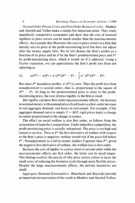
Second-Order Private Costs and First-Order Business Cycles. Mankiw and Akerlof and Yellen make a simple but important point. They study imperfectly competitive economies and show that the cost of nominal rigidities to price setters can be much smaller than the macroeconomic effects. An example that illustrates the cost to price setters is a firm that initially sets its price at the profit-maximizing level but does not adjust after the money supply falls. We let -r(-) denote the firm's profits as a function of its price and let P be the firm's predetermined price and P* its profit-maximizing price, which it would set if it adjusted. Using a Taylor expansion, we can approximate the firm's profit loss from not adjusting as

(1) IT(P*) - i,(P) U'(p*)(p* - P) - 1i T" (P*)(P* - P)2. 2

But since P* maximizes profits, -a'(P*) is zero. Thus the profit loss from nonadjustment is second order-that is, proportional to the square of (P* - P). As long as the predetermined price is close to the profit- maximizing price, the cost of price rigidity to the firm is small.

But rigidity can have first-order macroeconomic effects. An increase in nominal money with nominal prices fixed leads to a first-order increase in real aggregate demand, and hence in real output. For example, if the aggregate demand curve is simply Y = MIP, rigid prices imply a change in output proportional to the change in money.

The effect on social welfare is also first order, as follows from the assumption of imperfect competition. Under imperfect competition, the profit-maximizing price is socially suboptimal. The price is too high and output is too low. Thus at P* the first derivative of welfare with respect to the firm's price is negative: welfare would rise if the piice fell below P*. Nonadjustment to a fall in money implies P greater than P*; given the negative first derivative of welfare, the welfare loss is first order.

Because the cost of rigidity to a price setter is second order while the macroeconomic effects are first order, the latter can be much larger. This finding resolves the puzzle of why price setters refuse to incur the small costs of reducing the business cycle through more flexible prices. Despite the large macroeconomic effects, the private incentives are small.

Aggregate Demand Externalities. Blanchard and Kiyotaki provide an important interpretation of the result in Mankiw and Akerlof-Yellen:

Laurence Ball, N. Gregoty Mankiw, and David Romer 7

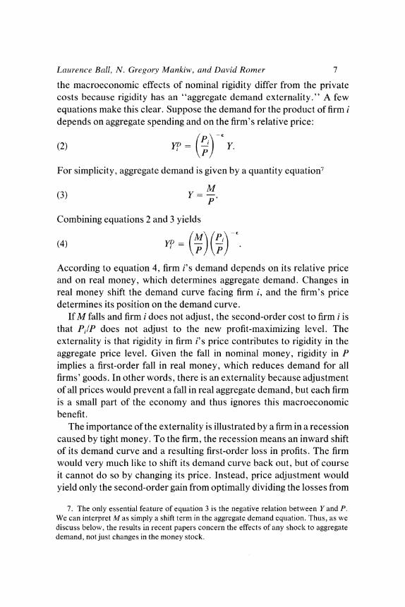
the macroeconomic effects of nominal rigidity differ from the private costs because rigidity has an "aggregate demand externality." A few equations make this clear. Suppose the demand for the product of firm i depends on aggregate spending and on the firm's relative price:

(2) Y= (p) Y

For simplicity, aggregate demand is given by a quantity equation7

(3) y M P

Combining equations 2 and 3 yields

(4) Y (p)(p E

According to equation 4, firm i's demand depends on its relative price and on real money, which determines aggregate demand. Changes in real money shift the demand curve facing firm i, and the firm's price determines its position on the demand curve.

If M falls and firm i does not adjust, the second-order cost to firm i is that PilP does not adjust to the new profit-maximizing level. The externality is that rigidity in firm i's price contributes to rigidity in the aggregate price level. Given the fall in nominal money, rigidity in P implies a first-order fall in real money, which reduces demand for all firms' goods. In other words, there is an externality because adjustment of all prices would prevent a fall in real aggregate demand, but each firm is a small part of the economy and thus ignores this macroeconomic benefit.

The importance of the externality is illustrated by a firm in a recession caused by tight money. To the firm, the recession means an inward shift of its demand curve and a resulting first-order loss in profits. The firm would very much like to shift its demand curve back out, but of course it cannot do so by changing its price. Instead, price adjustment would yield only the second-order gain from optimally dividing the losses from

7. The only essential feature of equation 3 is the negative relation between Y and P. We can interpret M as simply a shift term in the aggregate demand equation. Thus, as we discuss below, the results in recent papers concern the effects of any shock to aggregate demand, not just changes in the money stock.

8 Br-ookinigs Papers on Economnic Activity, 1:1988

the recession between reduced sales and a lower price. The recession would end and everyone would be much better off if all firms adjusted. But each firm believes that it cannot end the recession and therefore may fail to adjust even if the costs of adjustment are much smaller than the costs of the recession.

This argument resembles standard microeconomic analyses of externalities. Consider the classic example of pollution. Pollution would be greatly reduced, and social welfare greatly improved, if each person incurred the small cost of walking to the trash can at the end of the block. But each individual ignores this when he throws his wrapper on the street because he is only one of many polluters. Because of externalities, economists do not find highly inefficient levels of pollution puzzling even though the costs of reducing pollution are small. For similar reasons, highly inefficient nominal rigidities are not a mystery even though menu costs are small.

Externalities from Fluctuations in Demand. Keynesians believe not only that shocks to nominal aggregate demand cause large fluctuations in output and welfare, but also that these fluctuations are inefficient, and thus that stabilization of demand is desirable. The models surveyed so far do not provide a foundation for this view. As explained above, nonadjustment of prices to a fall in demand leads to large reductions in output and welfare. But nonadjustment to a rise in demand leads to higher output and, because output is initially too low under imperfect competition, to higher welfare. Thus the implications of fluctuations for average welfare, and hence the desirability of reducing fluctuations, are unclear. Indeed, Ball and Romer show that the first-order welfare effects of fluctuations average to zero, which means that the first order-second order distinction is irrelevant to this issue.8

Nonetheless, Ball and Romer show, by comparing the average social and private costs of nominal rigidity, that small nominal frictions are sufficient for large reductions in average welfare. The private cost is fluctuations of a firm's relative price around the profit-maximizing level. The social cost is the private cost plus the cost of fluctuations in real aggregate demand. Greater flexibility would stabilize real demand, but each firm ignores its effect on the variance of demand, just as it ignores its effect on the level of demand after a given shock. Although both the

8. Ball and Romer, "Are Prices Too Sticky?"

Laiurence Ball, N. Gregory Mankiw, and David Romner- 9

average social and average private costs are second order, Ball and Romer show that the former may be much larger: fluctuations in aggregate demand can be much more costly than fluctuations in relative prices. As a result, small frictions can prevent firms from adopting greater flexibility even if business cycles are highly inefficient.

STILL LARGER RIGIDITIES

The papers discussed so far establish that nominal rigidities can be far larger than the frictions that cause them. But as we now describe, the simple models in these papers cannot fully explain nonneutralities of the size and persistence observed in actual economies. Therefore, we turn to more complicated models that incorporate realistic phenomena that magnify nominal rigidities. These phenomena include rigidities in real wages and prices and asynchronized timing of price changes by different firms.

Real Rigidities. As we argue above, real rigidities alone are no impediment to full nominal flexibility. But Ball and Romer show that a high degree of real rigidity, defined as small responses of real wages and real prices to changes in real demand, greatly increases the nonneutralities arising from small nominal frictions.9

This finding is important because, although models with nominal frictions but no real rigidities can in principle produce large nominal rigidities, they do so only for implausible parameter values. Most important, large rigidities arise only if labor supply is highly elastic, while labor supply elasticities in actual economies appear small. The role of labor supply is illustrated by a hypothetical economy with imperfect competition and menu costs in the goods market but a Walrasian labor market. If menu costs led to nominal price rigidity, then nominal shocks would cause large shifts in labor demand. But if labor supply were inelastic, these shifts in labor demand would cause large changes in the real wage and thereby create large incentives for price setters to adjust their prices. As a result, nominal rigidity would not be an equilibrium.

While for plausible parameter values nominal frictions alone produce little nominal rigidity, Ball and Romer show that considerable rigidity

9. Laurence Ball and David Romer, "Real Rigidities and the Non-Neutrality of Money," Working Paper 2476 (NBER, December 1987).

10 Brookings Paper-s on Economic Activity, 1:1988

can arise if the frictions are combined with real rigidities arising from efficiency wages, customer markets, and the like. For example, substantial nominal rigidity can arise from a combination of real rigidity in the labor market and imperfect competition and menu costs in the goods market. If firms pay efficiency wages, for instance, then real wages may be set above the market-clearing level, so that workers are off their labor supply curves. In this situation a fall in labor demand can greatly reduce employment without a large fall in the real wage even if labor supply is inelastic.

The importance of real rigidities for explaining nominal rigidities is not settled, because there is no consensus about the sources and magnitudes of real rigidities in actual economies. In particular, phenomena like efficiency wages and customer markets increase nominal rigidity to the extent that they reduce desired responses of real wages and real prices to demand shifts, but economists are still unsure of the sizes of these effects. Further research on real rigidities will lead to a better understanding of nominal rigidities.

Staggered Price Setting. Even when real rigidities are added, the models surveyed so far cannot fully explain the size and persistence of the real effects of nominal shocks. In these models, the effects of shocks are eliminated when nominal prices adjust. In actual economies, reces- sions following severe demand contractions can last for several years, and while individual prices are fixed for substantial periods, these periods are generally shorter than several years. Thus models with sticky prices must explain why the effects of shocks persist after all prices are changed.

An explanation is provided by the literature on staggered price setting, which shows that if firms change prices at different times, the adjustment of the aggregate price level to shocks can take much longer than the time between adjustments of each individual price. 10 The "price level inertia" caused by staggering implies that nominal shocks can have large and long-lasting real effects even if individual prices change frequently.

10. John B. Taylor, "Staggered Wage Setting in a Macro Model," American Economic Review, vol. 69 (May 1979, Papers andProceedings, 1978), pp. 108-13; Taylor, "Aggregate Dynamics and Staggered Contracts," Journal of Political Economy, vol. 88 (February 1980), pp. 1-23; Olivier J. Blanchard, "Price Asynchronization and Price Level Inertia," in Rudiger Dornbusch and Mario Henrique Simonsen, eds., Inflation, Debt, andIndexation (MIT Press, 1983), pp. 3-24; Olivier J. Blanchard, "The Wage Price Spiral," Quarterly Journal of Economics, vol. 101 (August 1986), pp. 543-65.

Lauirence Ball, N. Gregory Mankiw, and David Romer 11

A simple example makes clear the importance of the timing of price changes. Suppose first that every firm adjusts its price on the first of each month, so that price setting is synchronized. If the money supply falls on June 10, output is reduced from June 10 to July 1, because nominal prices are fixed during this period. But on July 1 all prices adjust in proportion to the fall in money, and the recession ends.

Now suppose that half of all firms set prices on the first of each month and half on the fifteenth. If the money supply falls on June 10, then on June 15 half the firms have an opportunity to adjust their prices. But in this case they may choose to make little adjustment. Because half of all nominal prices remain fixed, adjustment of the other prices implies changes in relative prices, which firms may not want. (In contrast, if all prices change simultaneously, full nominal adjustment does not affect relative prices.) If the June 15 price setters make little adjustment, then the other firms make little adjustment when their turn comes on July 1, because they do not desire relative price changes either. And so on. The price level declines slowly as the result of small decreases every first and fifteenth, and the real effects of the fall in money die out slowly. In short, price adjustment is slow because neither group of firms is willing to be the first to make large cuts. 11

As Blanchard emphasizes, if staggering occurs among firms at different points in a chain of production, its effects are strengthened.12 A

11. A natural question is why firms change prices at different times if this exacerbates aggregate fluctuations. One obvious answer is that different firms receive shocks at different times and face different costs of price adjustment. Laurence Ball and David Romer, "The Equilibrium and Optimal Timing of Price Changes," Working Paper 2412 (NBER, October 1987), show that, because of externalities from staggering, idiosyncratic shocks can lead to staggering even if synchronized price setting is Pareto superior. But idiosyncratic shocks cannot explain all staggering. For example, some firms with two-year labor contracts set wages in even years and some set them in odd years, and this does not correspond to deterministic two-year cycles in the arrival of shocks. Another explanation for staggering is that it arises from firms' efforts to gain information. This source of staggering is discussed in Arthur M. Okun, Prices and Quantities: A Macroeconomic Analysis (Brookings, 1981), and formalized in Laurence Ball and Stephen G. Cecchetti, "Imperfect Information and Staggered Price Setting," Working Paper 2201 (NBER, April 1987). For example, a firm wants to set wages in line with the wages of other firms. If all wages are set simultaneously, each firm is unsure of what wage to set because it does not know what others will do. This gives each firm an incentive to set its wage shortly after the others. The desire of each firm to "bat last," as Okun puts it, can lead in equilibrium to a uniform distribution of signing dates.

12. Blanchard, "Price Asynchronization."

12 Brookings Paipers on Economic Activity, 1:1988

firm's profit-maximizing price is tied to both the prices of its inputs and the prices of goods for which its product is an input (the latter influence demand for the firm's product). Thus a firm does not want to adjust its price to a shock if these other prices do not adjust at the same time. This reluctance to make asynchronized adjustments causes price level inertia. Blanchard shows that the degree of inertia increases the longer the chain of production: it takes a long time for the gradual adjustment of prices to make its way through a complicated system.

The literature on staggered price setting complements that on nominal rigidities arising from menu costs. The degree of rigidity in the aggregate price level depends on both the frequency and the timing of individual price changes. Menu costs cause prices to adjust infrequently. For a given frequency of individual adjustment, staggering slows the adjustment of the price level. Large aggregate rigidities can thus be explained by a combination of staggering and nominal frictions: the former mag- nifies the rigidities arising from the latter.

Asymmetric Effects ofDemand Shocks. We conclude this part of our discussion by mentioning a little-explored possibility for strengthening Keynesian models. The models surveyed imply symmetric responses of the economy to rises and falls in nominal aggregate demand. For example, in menu cost models the range of shocks to which prices do not adjust is symmetric around zero, and so is the range of possible changes in output. But traditional Keynesian models often imply asymmetric effects of demand shifts. In undergraduate texts, for example, the aggregate supply curve is often drawn so that decreases in demand lead to large output losses while the effects of increases are mostly dissipated through higher prices. Such asymmetries are intuitively appealing, and they greatly strengthen the Keynesian view that demand stabilization is desirable: stabilization raises the average levels of output and employment as well as reducing the variances. It is unclear whether plausible modifications of new Keynesian models can produce asymmetries. Asymmetric effects of shocks could arise from asymmetric price rigidity-prices that are sticky downward but not upward-but this is another appealing notion that is difficult to formalize. 3

13. Timur Kuran shows that asymmetries in firms' profit functions, which many menu cost models ignore, can lead to asymmetric price rigidity. But the asymmetries appear small. See Timur Kuran, "Asymmetric Price Rigidity and Inflationary Bias," American Economic Reviewv, vol. 73 (June 1983), pp. 373-82; Kuran, "Price Adjustment Costs,

Laiurence Ball, N. Gregory Mankiw, and David Roiner 13

THE NEW ASSUMPTIONS IN NEW KEYNESIAN MODELS

Aside from the specific arguments outlined above, recent research establishes the general point that nominal rigidities can result from optimizing choices of agents in well-specified models. This contrasts with the ad hoc imposition of rigidities in many of the Keynesian models of the 1970s. Recent progress is largely a result of two innovations in modeling: the introduction of imperfect competition and greater emphasis on price rather than wage rigidities.

Imperfect Competition. Microeconomists have long recognized that sticky prices and perfect competition are incompatible. 14 In a competitive market, a firm does not set its price, but accepts the price quoted by the Walrasian auctioneer. Only under imperfect competition, when firms set prices, does it make sense to ask whether a firm adjusts its price to a shock. Nonetheless, Keynesian models of the 1970s, most clearly disequilibrium models, imposed nominal rigidities on otherwise Walras- ian economies. The result was embarrassments in the form of unappealing results or the need for additional arbitrary assumptions. Many recent models simply generalize earlier models by allowing the firms' demand curves to slope down. This single modification sweeps away many of the problems with older models. Specifically, the new models with imperfect competition offer six advantages:

-Private costs of rigidity are second order. Under perfect competition, the gains from nominal adjustment are large. For example, if nominal demand rises and prices do not adjust, there is excess demand. In this situation, an individual firm can raise its price significantly and still sell as much output as before, which implies a large increase in profits. In contrast, under imperfect competition a higher price always implies lower sales. Starting from the profit-maximizing price-qllantity combination, the gains from trading off price and sales after a shc-k are second order.

Anticipated Inflation, and Output," Quarterly Journal of Economics, vol. 101 (May 1986), pp. 407-18.

14. See, for example, Kenneth J. Arrow, "Toward a Theory of Price Adjustment," in Moses Abramovitz and others, eds., The Allocation of Economic Resources: Essays in Honor of Bernard Francis Haley (Stanford University Press, 1959), pp. 41-5 1.

14 Br-ookings Paper-s on Economic Activity, 1:1988

-Output is demand determined. When price rigidity is imposed on a Walrasian market, so that the market does not clear, it is natural to assume that quantity equals the smaller of supply and demand, so that output falls below the Walrasian level when price is either above or below the Walrasian level. But Keynesians believe that when prices are rigid, increases in demand, which mean prices below Walrasian levels, raise output, just as decreases in demand reduce output. This result is built into many Keynesian models through the unappealing assumption that output is demand determined even if demand exceeds supply. For example, in the Gray-Fischer contract model, firms hire as much labor as they want, regardless of the preferences of workers.15 In contrast, under imperfect competition, demand determination arises naturally. Firms set prices and then meet demand. Crucially, if demand rises, firms are happy to sell more even if they do not adjust their prices, because under imperfect competition price initially exceeds marginal cost. Thus changes in demand always cause changes in output in the same direction.

-Booms raise welfare. Under perfect competition, the equilibrium level of output in the absence of shocks is efficient. Thus increases in output resulting from positive shocks, as well as decreases resulting from negative shocks, reduce welfare. In the Gray-Fischer model, for example, half the welfare loss from the business cycle occurs when workers are required to work more than they want. In actual economies, unusually high output and employment mean that the economy is doing well.16 And this is the case in models of imperfect competition. Since imperfect competition pushes the no-shock level of output below the social optimum, welfare rises when output rises above this level.

-Wage rigidity causes unemployment through low aggregate demand. In 1970s models with sticky nominal wages, unemployment occurs when prices fall short of the level expected when wages were set, so that real wages rise and firms move up their labor demand curves. In actual economies, however, firms often appear to reduce employment because demand for their output is low, not because real wages are high. This fact is not necessarily a problem for Keynesian theories if the goods market is imperfectly competitive. In this case, a firm's labor demand

15. Fischer, "Long-Term Contracts," and Gray, "On Indexation." 16. Of course economists worry that low unemployment may be inflationary. But

sticky-price models with perfect competition imply that low unemployment is undesirable per se.

Laiur-ence Ball, N. Gregoty Mankiw, and David Romer 15

depends on real aggregate demand as well as the real wage, because changes in aggregate demand shift the firm's product demand (see equation 2).

-Real wages need not be countercyclical. Imperfect competition can remedy an embarrassing empirical failure of traditional models based on sticky nominal wages-the cyclical behavior of real wages. We can tautologically write P = pWIMPL, where P is the price level, W is the wage, MPL is the marginal product of labor, and p is the markup of price over marginal cost. If the markup is constant and marginal prodtuct of labor is diminishing, as many 1970s models assumed, then the real wage, WIP = MPLI,u, must be countercyclical. In actual economies, however, real wages appear acyclical or abit procyclical. This fact can be explained if the marginal product of labor is constant, as suggested by Hall, or if the markup is countercyclical. as suggested by Rotemberg and Saloner and by Bils. 7 Thus there need not be a link between changes in employment and changes in real wages.

-Nominal rigidities have aggregate demand externalities. As we have explained, since real aggregate demand affects the demand curves facing individual firms, nominal rigidities have externalities. Rigidity in one firm's price contributes to rigidity in the price level, which causes fluctuations in real aggregate demand and thus harms all firms. These externalities are crucial to the finding that small frictions can have large macroeconomic effects. The externalities depend on imperfect competition, for under perfect competition, aggregate demand is irrelevant to individual firms because they can sell all they want at the going price.

ProduictMarketRigidities. Keynes and most Keynesians emphasize rigidities in nominal wages. But recent work focuses largely on rigidities in product prices. The change offers two advantages.

-Goods are sold in spot markets. Although there is clearly much nominal wage rigidity in actual economies-in U.S. labor contracts, for example, wages are set up to three years in advance-the allocative effects of this rigidity are unclear. The implicit contracts literature shows that it may be efficient for contract signers to make employment

17. Robert E. Hall, "Market Structure and Macroeconomic Fluctuations," BPEA, 2: 1986, pp. 285-322; Julio J. Rotemberg and Garth Saloner, "A Supergame-Theoretic Model of Price Wars during Booms," American Econiomic Review, vol. 76 (June 1986), pp. 390-407; Mark Bils, "Cyclical Pricing of Durable Luxuries," Working Paper 83 (University of Rochester Center for Economic Research, May 1987).


independent of wages. That is, given long-term relationships with their workers, firms may choose the efficient amount of employment rather than moving along their labor demand curves when real wages change. 18 In many product markets, on the other hand, buyers clearly operate on their demand curves. For example, the local shoe store has no agreement, explicit or implict, from its customers to buy the efficient number of shoes regardless of the prices. Instead, rigidity in the store's prices affects its sales of shoes.

-Real wages need not be countercyclical. As we argue above, acyclical real wages are possible even if nominal rigidities occur only in wages. But it is easiest to explain acyclical or procyclical real wages if prices as well as wages are sticky. In this case, the effect of a shock on real wages depends on the relative sizes of the adjustments of prices and wages.

Despite the advantages of studying rigidities in goods markets, we are ambivalent about the deemphasis of labor markets, because the apparent rigidities in nominal wages may have important allocative effects. Further research on the relative importance of wage and price rigidities is needed.

DISCUSSION

We conclude this section by discussing several issues concerning the importance of recent theories and their plausibility.

The Importance of Nominal Rigidities. Nominal rigidities are essential for explaining important features of business cycles. As we have emphasized, real effects of nominal disturbances, such as changes in the money stock, depend on some nominal imperfection. The only prominent alternative to nominal rigidities is imperfect information about the aggregate price level, an explanation that many economists find implausible. It is possible, of course, to maintain that money is neutral in the short run-that Paul Volcker, for example, had nothing to do with the 1982 recession-but this also appears unrealistic to many economists.

18. Early expositions ofthis ideaappearin Martin Neil Baily, "Wages and Employment under Uncertain Demand," Review of Economic Studies, vol. 41 (January 1974), pp. 37- 50; Costas Azariadis, "Implicit Contracts and Underemployment Equilibria," Journal of Political Economy, vol. 83 (December 1975), pp. 1183-1202; and Robert E. Hall, "The Rigidity of Wages and the Persistence of Unemployment," BPEA, 2:1975, pp. 301-35.

Lautrence Ball, N. Gregoty Mankiw, and David Rower 17

Thus it is difficult to explain the relation of output to nominal variables without nominal rigidities.

Nominal rigidities are also important for explaining the effects of real shocks to aggregate demand, resulting, for example, from changes in government spending or in the expectations of investors. The point is clear if we interpret M in the aggregate demand equation, Y = MIP, as simply a shift term, in which case real disturbances that shift demand affect output through the same channels as changes in money.

Not all explanations for the output effects of real demand shocks depend on nominal imperfections. Robert Barro's model of government purchases, for one, does not. 19 But such explanations invoke implausibly large labor supply elasticities. Thus nominal rigidities, while not the only explanation for the effects of real demand, are perhaps the most appealing.

In the models we have surveyed, slow adjustment of prices implies that shocks cause temporary deviations of output and employment from their "natural rates. " Recently, however, models of hysteresis, in which shocks have permanent effects, have become popular. For example, Blanchard and Summers argue that the natural rate of unemployment in European countries changes when actual unemployment changes, so that there is no unique level to which unemployment returns.20 If these theories are correct, then nominal rigidities cannot fully explain unemployment, because nominal prices eventually adjust to shocks; some additional explanation, such as the insider-outsider model in Blanchard and Summers, is needed for the persistence of unemployment. But nominal rigidities may be crucial for explaining the initial impulses in unemployment. For example, after rising during the late 1970s, unemployment in Britain has remained high, suggesting hysteresis. But the best explanation for the original increase is arguably a conventional one: slow adjustment of wages and prices to shocks like tight monetary policy and increases in import prices.

The Importance of Externalities from Rigidity. Externalities from nominai rigidity, the central element of menu cost models, are essential

19. Robert J. Barro, "Output Effects of Government Purchases," Journal of Political Economy, vol. 89 (December 1981), pp. 1086-1121.

20. Olivier J. Blanchard and Lawrence Summers, "Hysteresis and the European Unemployment Problem," in Stanley Fischer, ed., NBER Macroeconomics Annual, 1986 (MIT Press, 1986), pp. 15-78.


for a plausible theory of rigidities. If rigidities exist, one of the following statements must be true: rigidities do not impose large costs on the economy; rigidities have large costs to the firms and workers who create them, but these are exceeded by the costs of reducing rigidities; or rigidities have small private costs, and so small frictions are sufficient to create them, but externalities from rigidity impose large costs on the economy. The problem with the first statement is the difficulty of explaining apparently costly events, such as rises in unemployment following monetary contractions, without nominal rigidities. The second seems implausible: it would not be costly for magazine publishers to print new prices every year rather than every four years, as they typically do.2" Thus the third statement is the best hope for explaining rigidities.

What Are Menu Costs? Models of nominal rigidity depend on some cost of full flexibility, albeit a small one. The term menu cost may be misleading because the physical costs of printing menus and catalogs may not be the most important barriers to flexibility. Perhaps more important is the lost convenience of fixing prices in nominal terms-the cost of learning to think in real terms and of computing the nominal price changes corresponding to desired real price changes. More generally, we can view infrequent revision of nominal prices as a rule of thumb that is more convenient than continuous revision. Thus, rather than referring to menus, we can state the central argument of recent papers as follows. Firms take the convenient shortcut of infrequently reviewing and changing prices. The resulting profit loss is small, so firms have little incentive to eliminate the shortcut, but externalities make the macroeconomic effects large.

At a somewhat deeper level, we can interpret the convenience of fixing nominal rather than real prices as that of using the medium of exchange, dollars, as a unit of account.22 Alternatively, following Akerlof and Yellen, we can view simple rules of thumb as arising from "near-

21. Stephen G. Cecchetti, "The Frequency of Price Adjustment: A Study of the Newsstand Prices of Magazines," Journal of Econometrics, vol. 31 (August 1986), pp. 255-74. The cost of reducing nominal wage rigidity may be significant if rigidity is reduced through shorter labor contracts, which require more frequent negotiations between unions and management. But wage rigidity can also be reduced through greater indexation or by having the nominal wage change more often over the life of a contract, neither of which appears to have large costs.

22. Bennett T. McCallum, "On 'Real' and 'Sticky-Price' Theories of the Business Cycle," Journal of Money, Credit, and Banking, vol. 18 (November 1986), pp. 397-414.

Lalurence Ball, N. Gregory Mankiw, and David Romer 19

rationality," a small departure from full optimization.23 In any case, the precise source of frictions is not important. The effects of nominal shocks are the same whether rigidity arises from printing costs, near-rationality, or something else.

Inflation, the Frequency of Adjustment, and the Phillips Curve

Recent research shows that nominal rigidity is possible in principle- that one can construct a model with firm microeconomic foundations in which rational agents choose substantial rigidity. But the validity of Keynesian theories is not thereby established. For these theories to be convincing, they must have empirical implications that contradict other macroeconomic theories, and these predictions must be confirmed by evidence. This section derives implications of recent Keynesian models, and the next section tests them. As explained in the introduction, the main prediction is that the real effects of nominal shocks are smaller when average inflation is higher. Higher average inflation erodes the frictions that cause nonneutralities, for example by causing more frequent wage and price adjustments.

This section studies a specific model of the class described in the previous section. In the model, a cost of price adjustment leads firms to change prices at intervals rather than continuously. In addition to providing a basis for the empirical tests of the next major section, the model is of theoretical interest. Previous models of nominal rigidity are highly stylized; for example, most menu cost models are static. Our model is dynamic and has the appealing feature that the price level adjusts slowly over time to a nominal shock. The speed of adjustment, which is treated as exogenous in older Keynesian models, is endogenous. It depends on the frequency of price adjustment by individual firms, which in turn is derived from profit-maximization.24

We first present the model and show that high average inflation reduces the output effects of nominal shocks. We also show that highly variable aggregate demand reduces these effects. We then investigate

23. Akerlof and Yellen, "A Near-Rational Model." 24. The speed of adjustment is also endogenous in Laurence Ball, "Externalities from

Contract Length," Amesrican Economic Review, vol. 77 (September 1987), pp. 615-29.


the model's quantitative implications by calculating the real effects of shocks for a range of plausible parameter values. The results suggest that the effects of average inflation and demand variability are large. Next we argue that the implications of our model are robust: they carry over to broad classes of other Keynesian models.

Finally, we compare the predictions of Keynesian theories with those of models in the new classical or equilibrium tradition, focusing on Lucas's model of imperfect information. Like our model, Lucas's predicts that the size of the real effects of shocks depends negatively on the variance of aggregate demand. Since this prediction is common to Keynesian and new classical theories, testing it empirically, as Lucas and others have done, is not useful for distinguishing between the two theories. Crucially, Lucas's model differs from ours by predicting that the effects of shocks do not depend on average inflation. This difference leads to the tests of the models in the next section.

THE MODEL AND QUALITATIVE RESULTS

Our model of price adjustment is similar in spirit to those of John Taylor and Olivier Blanchard.25 The model is set in continuous time. The economy contains imperfectly competitive firms that change prices at discrete intervals rather than continuously, because adjustments are costly. Price setting is staggered, with an equal proportion of firms changing prices at every instant. The crucial departure from Taylor and Blanchard is that the length of time between price changes, and hence the rate at which the price level adjusts to shocks, is endogenous. Thus we can study the determinants of the speed of adjustment.

Consider the behavior of a representative firm, firm i. Rather than derive a profit function from specific cost and demand functions, we simply assume that firm i's profits depend on three variables: aggregate spending in the economy, y; firm i's relative price, pi - p; and a firm- specific shock, Oi (all variables are in logs). The aggregate price level p is defined simply as the average of prices across firms. Aggregate spending y affects firm i's profits by shifting the demand curve that it faces. When aggregate spending rises, the firm sells more at a given

25. Taylor, "Staggered Wage Setting" and "Aggregate Dynamics and Staggered Contracts"; and Blanchard, "Price Asynchronization" and "Wage Price Spiral."

Lauirence Ball, N. Gregory Mankiw, and David Romer 21

relative price. The term pi - p affects the firm's profits by determining the position on the demand curve at which it operates. And Oi is an idiosyncratic shock to either demand or costs (the presence of Oi is not needed for our main qualitative results, but it strongly affects the quantitative results of the next section).

We assume that the elasticity of firm i's profit-maximizing real price, Pi - p, with respect to y is a positive constant, v. Without loss of generality, we assume that the elasticity of pi - p with respect to Oi is one, and that Oi has zero mean. Thus we can write the profit-maximizing real price as

(5) Pi (t) - p(t) = v[y(t) - y(t)] + Oi(t), v > 0,

where y is the natural rate of output-the level at which, if Oi equals its mean, the firm desires a relative price of one. (Relative prices equal to one is the condition for a symmetric equilibrium of the economy when prices are flexible.)26

If price adjustment were costless, firm i would set pi = pi at every instant. We assume, however, that an adjustment cost leads firms to change prices only at intervals of length X, which for simplicity is constant over time (later in this section we discuss the implications of allowing X to vary). Specifically, each price change has a fixed cost F, so adjustment costs per period are FIX.

As noted above, an equal proportion of firms sets prices at every instant.27 If firm i sets a price at t, it chooses the price and A to maximize its expected profits, averaged over the life of the price (from t to t + X). Maximizing profits is equivalent to minimizing profit losses from two sources: adjustment costs and deviations of price from the profit-

26. As an example of foundations for equation 5, suppose that firm i's demand equation is Yi = y - E(Pi - p) (demand depends on aggregate spending and the firm's relative price), and that its log costs are yyi + (1 - e + Ey)Oi. This implies equation 5 with v = (y - 1)/ (1 - e + Ey) and - = [1/(y - 1)] ln [(e - 1)/Ey] (the coefficient on Oi in the cost function is chosen to satisfy the normalization that the coefficient on Oi in equation 5 is one). For deeper microfoundations, see Ball and Romer, "Equilibrium and Optimal Timing of Price Changes," where a price-setting rule like equation 5 is derived from utility and production functions.

27. We assume that price setting is staggered so that inflation is smooth. If all firms changed prices at the same times, the aggregate price level would remain constant between adjustments and thenjump discretely. We do not model the sources of staggering explicitly; for explanations of staggering, see the references in note 11.


maximizing level. We approximate the latter by 1 K (pi - p*)2, where K is the negative of the second derivative of profits with respect to pi - pi. Thus firm i's loss per unit of time is

(6) F + !!K Et [pi (t + s) PJ2 ds x + =

Minimization of equation 6 implies a simple rule for choosing pi:

(7) Pi = , Et p (t + s)ds.

That is, a firm sets its price to the average of its expected profit- maximizing prices for the period when the price is in effect. We describe the more complicated determination of X below.

To study the effects of nominal shocks, we must introduce a stochastic nominal variable. We assume that the log of nominal aggregate demand, x =y + p, is exogenous and follows the continuous-time analogue of a random walk with drift:

(8) x(t) = gt + o>XW(t),

where W(t) is a Wiener process. The first term in the expression for x(t) captures trend growth of g per unit time; the second captures random walk innovations with variance (o2 per unit time. Our analysis below focuses on the effects of the parameters g and a-x on the economy. A monetarist interpretation of equation 8 is that x(t) = m(t) + V-the velocity of money is constant, and aggregate demand is driven by random walk movements in the money stock. A more general interpretation is that a variety of exogenous variables-fiscal policy, the expectations of investors, and so on-drive x(t).

We make two final assumptions. First, the natural rate of output grows smoothly at rate p,:

(9) y-(t)= =, t.

Along with the process for x(t), this implies that average inflation is g - p,. Second, the firm-specific disturbances, the Oi's, are uncorrelated across firms and follow continuous-time random walks whose innovations have mean zero and variance ao per unit time.28

28. More precisely, we assume that Oi follows a stationary process and consider the limit as this process approaches a random walk. (If Oi is a random walk, its mean is undefined, which contradicts our earlier assumption that its mean is zero.)


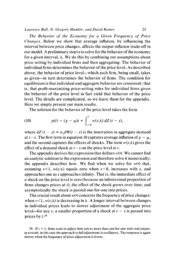
The Behavior of the Economy for a Given Frequency of Price Changes. Below we show that average inflation, by influencing the interval between price changes, affects the output-inflation trade-off in our model. A preliminary step is to solve for the behavior of the economy for a given interval, X. We do this by combining our assumptions about price setting by individual firms and then aggregating. The behavior of individual firms determines the behavior of the price level. As described above, the behavior of price level-which each firm, being small, takes as given-in turn determines the behavior of firms. The condition for equilibrium is that individual and aggregate behavior are consistent; that is, that profit-maximizing price-setting rules for individual firms given the behavior of the price level in fact yield that behavior of the price level. The details are complicated, so we leave them for the appendix. Here we simply present our main results.

The solution for the behavior of the price level takes the form

(10) p(t) = (g - )t + f w(s;X) dZ (t -s),

where dZ (t - s) - >dW(t - s) is the innovation in aggregate demand at t - s. The first term in equation 10 captures average inflation of g - PI , and the second captures the effects of shocks. The term w(s;X) gives the effect of a demand shock at t - s on the price level at t.

The appendix derives the expression that defines w(.). We cannot find an analytic solution to the expression and therefore solve it numerically; the appendix describes how. We find when we solve for w(.) that, assuming v<1, w(s;X) equals zero when s=O, increases with s, and approaches one as s approaches infinity. That is, the immediate effect of a shock on the price level is zero (because an infinitesimal proportion of firms changes prices at t); the effect of the shock grows over time; and asymptotically the shock is passed one-for-one into prices.

The crucial result about w(.) concerns the frequency of price changes: when v< 1, w(s;X) is decreasing in X. A longer interval between changes in individual prices leads to slower adjustment of the aggregate price level-for any s, a smaller proportion of a shock at t - s is passed into prices by t.29

29. If v > 1, firms want to adjust their prices more than one-for-one with real output; as a result, in this case the approach to full adjustment is oscillatory. The response is again slower when the frequency of price adjustment is lower.


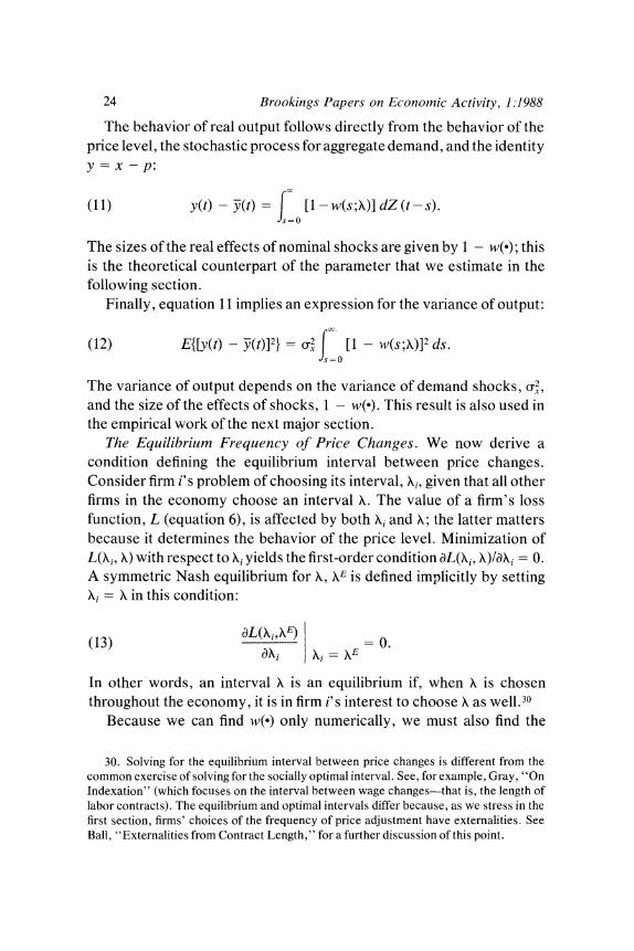
The behavior of real output follows directly from the behavior of the price level, the stochastic process for aggregate demand, and the identity y = x -p:

( 1 1 ) y((t) - = f [1 - w(s;X)] dZ (t - s). = =o

The sizes of the real effects of nominal shocks are given by 1 - w(.); this is the theoretical counterpart of the parameter that we estimate in the following section.

Finally, equation 11 implies an expression for the variance of output:

(12) E{[y(t) -y ] f [1 - w(s;X)]2ds. s=0

The variance of output depends on the variance of demand shocks, 02,

and the size of the effects of shocks, 1 - w(.). This result is also used in the empirical work of the next major section.

The Equilibrium Frequency of Price Changes. We now derive a condition defining the equilibrium interval between price changes. Consider firm i's problem of choosing its interval, Xi, given that all other firms in the economy choose an interval X. The value of a firm's loss function, L (equation 6), is affected by both Xi and X; the latter matters because it determines the behavior of the price level. Minimization of L(Xi, X) with respect to Xi yields the first-order condition aL(Xi, X)/axi = 0. A symmetric Nash equilibrium for X, XE is defined implicitly by setting Xi = X in this condition:

(13) ) | 0.

In other words, an interval X is an equilibrium if, when X is chosen throughout the economy, it is in firm i's interest to choose X as well.30

Because we can find w(.) only numerically, we must also find the

30. Solving for the equilibrium interval between price changes is different from the common exercise of solving for the socially optimal interval. See, for example, Gray, "On Indexation" (which focuses on the interval between wage changes-that is, the length of labor contracts). The equilibrium and optimal intervals differ because, as we stress in the first section, firms' choices of the frequency of price adjustment have externalities. See Ball, "Externalities from Contract Length," for a further discussion of this point.


equilibrium X numerically, as described in the appendix. We find that X is decreasing in i, o-x, and ao., where iT- g - p, is the average inflation rate. Thus the interval between price changes decreases the higher average inflation. High inflation causes a firm's profit-maximizing nominal price to change rapidly, which raises the benefits from frequent adjustment. The interval X also decreases the greater the variances of aggregate and firm-specific shocks. When either variance is large, a firm's future profit-maximizing price is highly uncertain, so the firm does not wish to fix its price for long.

These results, along with the results about the effects of X, imply that the Phillips curve is steeper when iT, o-a, or ar is larger. Higher average inflation reduces the interval between price changes, which in turn raises w(.), the proportion of a shock that is passed into prices. A larger variance of aggregate or firm-specific shocks also reduces X and thus raises w(.). These results imply that increases in iT, a-,, or ar lead to decreases in 1 - w(.), the real effects of shocks. These predictions lead to the empirical tests of the next section.

QUANTITATIVE RESULTS

We now ask whether the effects of inflation and demand variability identified above are quantitatively important. We do so by computing the interval between price changes and the real effects of shocks for a range of plausible parameter values.

Choice of Parameters. Since our focus is the effects of average inflation, g - [t, and the standard deviation of demand, a.., we experiment with wide ranges of values of these parameters (g and p affect the results only through their difference). This leaves three other parameters for which we need baseline values: F/K, the ratio of the cost of changing prices to the negative of the second derivative of the profit function (F and K enter only through their ratio); ur, the standard deviation of firm- specific shocks; and v, the elasticity of a firm's profit-maximizing real price with respect to aggregate output.

We choose baseline parameters by experimenting with values of F/K, uo, and v to find a combination that implies plausible sizes for the real effects of shocks. We then ask whether these parameter values are realistic. Finally, we investigate robustness by calculating the effects of changing each parameter from its baseline value.


It is difficult to measure F and K directly, so we take an indirect approach. In a model of steady inflation and no shocks (ur = ur = 0), F/K determines the frequency of price changes. With F/K = 0.00015, firms change prices every five quarters under steady 3 percent inflation and every two quarters under steady 12 percent inflation. Microeconomic evidence suggests that actual intervals between price changes typically average two years or more. Thus our baseline value of F/K is conserva- tive. We certainly do not assume menu costs that are too large to be consistent with price setting in actual economies.31

To pick a value for uo, we use the fact that uzr equals the standard deviation of movements in profit-maximizing prices, the p*'s, across firms. This leads us to use data on relative price variability to gauge plausible values of ur. Vining and Elwertowski report a 4-5 percent standard deviation of annual relative price movements across highly disaggregate (8-digit) components of the U.S. consumer price index; this is consistent with our assumption of uO = 3 percent.32

Finally, there is little quantitative evidence concerning the size of v, the elasticity of profit-maximizing relative prices with respect to aggregate output. However, our choice of a small elasticity, 0. 1, is consistent with the common view that relative prices vary little in response to aggregate fluctuations. Our baseline parameters are therefore F/K 0.00015, uo = 3 percent, and v = 0.1.

Results. Table 1 shows the effects of average inflation, g - VL, and the variability of demand, u, when F/K, u., and v equal their baseline values. For wide ranges of g - pL and u, the table shows two figures.

31. For microeconomic evidence on price behavior, see Cecchetti, "The Frequency of Price Adjustment"; Anil K. Kashyap, "Sticky Prices: New Evidence from Retail Catalogs" (MIT, November 1987); and W. A. H. Godley and C. Gillion, "Pricing Behavior in Manufacturing Industry," National Institute Economic Review, no. 33 (August 1965),

pp. 43-47. 32. Daniel R. Vining, Jr., and Thomas C. Elwertowski, "The Relationship between

Relative Prices and the General Price Level," American Economic Review, vol. 66 (September 1976), pp. 699-708. As a measure of r0, Vining and Elwertowski's figure has both an upward and a downward bias. The upward bias occurs because staggered price adjustment causes actual prices, the pi's, to vary across firms even when profit-maximizing prices, the p!'s, do not. As a result, the standard deviation of pi, which Vining and Elwertowski measure, is greater than the standard deviation of pi*, which equals r0. The negative bias in that variation across components of the CPI, even if these are highly disaggregated, is less than variation across individual prices. It is difficult to tell the relative magnitudes of these biases.

Lauzlrence Ball, N. Gregory Mankiw, and David Romner 27

Table 1. Effect of a Nominal Shock on Real Output and the Equilibrium Interval between Price Changes a

Average inflation

rate, Demand variability, Co (percent) g-[ x

(percent) 0 1 3 5 10 20

0 0.560 0.540 0.495 0.424 0.250 0.078 (31) (30) (28) (25) (17) (10)

2 0.519 0.519 0.470 0.405 0.250 0.078 (29) (29) (27) (24) (17) (10)

5 0.424 0.424 0.405 0.366 0.224 0.078 (25) (25) (24) (22) (16) (10)

10 0.322 0.322 0.299 0.299 0.199 0.078 (20) (20) (19) (19) (15) (10)

20 0.174 0.174 0.174 0.174 0.124 0.057 (14) (14) (14) (14) (12) (9)

50 0.057 0.057 0.057 0.057 0.039 0.023 (9) (9) (9) (9) (8) (7)

100 0.012 0.012 0.012 0.012 0.012 0.012 (6) (6) (6) (6) (6) (6)

250 0.001 0.001 0.001 0.001 0.001 0.001 (4) (4) (4) (4) (4) (4)

Source: Authors' calculations. See text description. a. The table shows the effects of changing values of g - p. and u. when FIK, uo, and v equal their baseline values.

F/K is the ratio of the cost of changing prices to minus the second derivative of the profit function; uro is the standard devialion of firm-specific shocks; and v is the elasticity of a firms profit-maximizing real price with respect to aggregate output. Baseline values: F/K = 0.00015; u0 = 3 percent; and v = 0.1. For each entry in the table, the first number is the percentage effect of a I percent nominal shock on real output after six months; the number in parentheses is the equilibrium interval between pnrce changes, X, in weeks.

The first is the percentage effect of a 1 percent change in demand on real output six months later. A value of zero would mean that prices adjust fully to the shock; a value of one would mean that prices do not adjust at all. We refer to this figure as simply the real effect of a shock. The figure in parentheses is the equilibrium interval between price changes, X, in weeks. As we explain above, inflation and demand variability influence the real effects of shocks through their effects on X.

Table 1 shows that realistic increases in average inflation have quantitatively important effects. With rO = 3 percent, roughly the standard deviation of nominal GNP growth for the postwar United States, the interval between price changes is 28 weeks if g - 1. = 0, but falls to 19 weeks if g - 1. = 10 percent and 6 weeks if g - 1. =- 100 percent. As a result, the real effect of a shock is 0.50 for g - 1. = 0, 0.30 for g - 1. = 10 percent, and 0.01 for g - 1. = 100 percent.

28 Brookings Papers oni Economic Activity, 1:1988

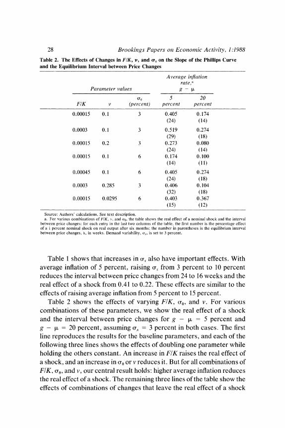
Table 2. The Effects of Changes in FIK, v, and c0 on the Slope of the Phillips Curve and the Equilibrium Interval between Price Changes

Aver-age ijiflation rate, a

Parameter val/tes g -

CFO 5 20 F/K v (percent) percent percent

0.00015 0.1 3 0.405 0.174 (24) (14)

0.0003 0.1 3 0.519 0.274 (29) (18)

0.00015 0.2 3 0.273 0.080 (24) (14)

0.00015 0.1 6 0.174 0.100 (14) (11)

0.00045 0.1 6 0.405 0.274 (24) (18)

0.0003 0.285 3 0.406 0.104 (32) (18)

0.00015 0.0295 6 0.403 0.367 (15) (12)

Source: Authors' calculations. See text description. a. For various combinations of F/K, v', and (ro, the table shows the real effect of a nominal shock and the interval

between price changes: for each entry in the last two columns of the table, the first number is the percentage effect of a i percent nominal sliock on real output after six months: the number in parentheses is the equilibrium interval between price changes, X, in weeks. Demand variability, arx, is set to 3 percent.

Table 1 shows that increases in (r, also have inmportant effects. With average inflation of 5 percent, raising ou, from 3 percent to 10 percent reduces the interval between price changes from 24 to 16 weeks and the real effect of a shock from 0.41 to 0.22. These effects are similar to the effects of raising average inflation from 5 percent to 15 percent.

Table 2 shows the effects of varying F/K, u., and v. For various combinations of these parameters, we show the real effect of a shock and the interval between price changes for g - 11 = 5 percent and g - 11 = 20 percent, assuming ou. = 3 percent in both cases. The first line reproduces the results for the baseline parameters, and each of the following three lines shows the effects of doubling one parameter while holding the others constant. An increase in FIK raises the real effect of a shock, and an increase in uo or v reduces it. But for all combinations of F/K, u0, and v, our central result holds: higher average inflation reduces the real effect of a shock. The remaining three lines of the table show the effects of combinations of changes that leave the real effect of a shock


unchanged for g - 11 = 5 percent. These lines show how the parameters affect the strength of the link between average inflation and the real effect of a shock.

ROBUSTNESS

Traditional Keynesian models, such as textbook models of price adjustment or the staggered contracts models of Fischer and Taylor, do not share the key predictions of our model.33 These older theories treat the degree of nominal rigidity (for example, the length of labor contracts or the adjustment speed of the price level) as fixed parameters; thus they rule out the channel through which average inflation affects the output- inflation trade-off. On the other hand, our central results appear to be robust implications of Keynesian theories in which the degree of rigidity is endogenous. The intuition for the effects of inflation on the frequency of price adjustment, and of this frequency on the size of nonneutralities, is not tied to the specific assumptions of our model.

One assumption of our model that requires attention is that the interval between price changes is constant over time. This assumption is ad hoc: given our other assumptions, firms could increase profits by varying the interval based on the realizations of shocks. In addition, the assumption is unrealistic, because firms in actual economies do not always change prices at fixed intervals.

We now consider the alternative assumption that firms can freely vary the timing of price changes. This assumption of complete flexibility is also far from realistic. Most wages are adjusted at constant intervals of a year. There appears to be greater flexibility in the timing of price changes, but the limited evidence suggests that it is not complete. Mail order companies change prices at fixed times during the year, even though they issue catalogs much more frequently than they change prices, and thus could vary the dates of adjustments without issuing extra catalogs. In addition, a broad range of industries appears to have a preferred time of the year, often January, for price changes.34

It is not yet possible to solve a model like ours with flexible timing,

33. For a textbook model, see Rudiger Dornbusch and Stanley Fischer, Macroeco- nomics, 4th ed. (McGraw-Hill, 1987).

34. For evidence on mail order catalogs, see Kashyap, "Sticky Prices." For evidence on industries' preferred months for price changes, see Julio J. Rotemberg and Garth Saloner, "A 'January Effect' in the Pricing of Goods" (MIT, 1988).

30 Br-ookings Paper s on Economfic Activity, 1 :1988

but suggestive results are available for simpler models. In particular, a literature beginning with Sheshinski and Weiss presents partial-equilibrium models in which a firm chooses to follow an "Ss" rule for adjusting its price: whenever inflation pushes its real price outside some bounds, it adjusts its nominal price to return the real price to a target level. These models reproduce a crucial implication of our model: higher average inflation leads to more frequent price changes. High inflation causes a firm's real price to change rapidly, so, for given Ss bounds, the price hits the bounds more often. High inflation also causes the firm to widen its bounds, which reduces the frequency of price changes, but does not fully offset the first effect.35

For our main argument to hold, the more frequent changes in individual prices that result from higher inflation must lead in turn to faster adjustment of the aggregate price level. Intuition clearly suggests a link between the frequency of individual adjustment and the speed of aggregate adjustment, but the difficulty of studying general equilibrium with flexible timing precludes a definitive proof. Indeed, in one prominent special case, the link does not exist. Andrew Caplin and Daniel Spulber show that if we assumne that firms follow Ss rules with constant bounds, and if aggregate demand is nondecreasing, then the aggregate price level adjusts immediately to nominal shocks-nominal shocks are neutral. Because aggregate adjustment is always instantaneous, its speed is obviously independent of the frequency of individual price changes.36

Current research suggests that the Caplin-Spulber result does not hold under realistic conditions. There exist examples in which firms do not follow Ss rules with constant bounds, and so a shock to the money supply is not neutral, either if there is some persistence to inflation or if firms' optimal nominal prices sometimes fall. And when nonneutralities exist, it appears plausible that their size depends on the frequency of individual price adjustment. Thus, overall, models of price adjustment with flexible timing appear consistent with the predictions of our model.37

35. The link between inflation and the frequency of adjustment is established for the case of constant inflation in Eytan Sheshinski and Yoram Weiss, "Inflation and Costs of Price Adjustment," Review of Economic Studies, vol. 44 (June 1977), pp. 287-303. An extension to the case of stochastic inflation is presented by Andrew S. Caplin and Eytan Sheshinski, "Optimality of (s, S) Pricing Policies" (Princeton University, 1987).

36. Andrew S. Caplin and Daniel F. Spulber, "Menu Costs and the Neutrality of Money," Quarterly Journal of Economics, vol. 102 (November 1987), pp. 703-25.

37. For the implications of persistent inflation, see Daniel Tsiddon, "On the Stubborn- ness of Sticky Prices" (Columbia University, July 1987). For the implications of falling

Lauirence Ball, N. Gregory Mankiw, and David Romner 31

Another robustness issue concerns the nature of the friction that prevents nominal flexibility. In our model, the friction is a fixed cost of price adjustment. An alternative view is that the technological costs of making prices highly flexible are negligible but that for some reason, such as convenience, the desire to avoid computation costs, or habit, price setters nonetheless follow rules that focus on nominal prices.38 Without a theory that predicts the particular rules of thumb that price setters follow, theories of this type do not make precise predictions concerning the relationship between average inflation and the degree of price flexibility. But it appears that under reasonable interpretations these theories imply that higher inflation increases nominal flexibility. As average inflation rises, so does the cost of following a rule-of-thumb pricing policy stated in nominal terms, as does the evidence that keeping a fixed nominal price is not equivalent to keeping a fixed real price. Although price setters may continue to follow rules of thumb, they will increasingly think in terms of real rather than nominal magnitudes. Nominal price flexibility will thus increase.

THE PREDICTIONS OF NEW CLASSICAL THEORIES

The prediction of Keynesian models that average inflation affects the output-inflation trade-off is important because it is inconsistent with alternative macroeconomic models in the new classical tradition. We now review the predictions of new classical models, focusing on Lucas's imperfect information theory. Like Keynesian models of nominal rigidity, Lucas's model is designed to explain the effects of nominal shocks on output-that is, to generate a short-run Phillips curve. But Lucas's model has different implications about what determines the size of the effects.

In Lucas's model, agents wish to change their output in response to changes in their relative prices, but not in response to changes in the aggregate price level. When an agent observes a change in his price, however, he cannot tell whether it results from a relative or an aggregate

optimal prices, see Blanchard, "Why Does Money Affect Output?" and Tsiddon, "The (Mis)behavior of the Aggregate Price Level" (Columbia University, 1987). These authors establish results for the special case in which a firm's optimal price moves one-for-one with aggregate demand and is independent of the price level (v = I in our notation).

38. See Akerlof and Yellen, "A Near-Rational Model."


movement. He acts upon his best guess, which is that part of the change comes from each source. Since agents interpret any price change as partly relative, changes that in fact result from a nominal shock have effects on output.

In Lucas's model, the size of the effects of nominal shocks depends on the relative magnitudes of nominal and idiosyncratic real shocks. In particular, if nominal shocks are large, agents attribute most of the movements in their prices to nominal shocks, and respond little. Thus a large variance of nominal aggregate demand leads to a steep Phillips curve. Lucas presents cross-country evidence supporting this prediction in his famous 1973 paper. We show, however, that Keynesian models make the same prediction, although the reason-a large variance of aggregate demand causes more frequent price changes-is very different. Because both Keynesian and new classical theories explain Lucas's results, his test does not help to distinguish between them.

The effect of average inflation on the output-inflation trade-off does distinguish Keynesian and new classical models. Theories of nominal rigidities predict that high inflation makes the Phillips curve steeper. In Lucas's imperfect information model, average inflation is irrelevant to the output-inflation trade-off, because only the variances of random variables, not the means, affect the uncertainty that agents face. This difference between the theories is the basis for our empirical work. (A simple correlation between average inflation and the slope of the Phillips curve is consistent with Lucas's model, because average inflation is correlated with the variance of demand, which affects the slope. Tne issue is whether there is a relation between average inflation and the slope after we control for the variance of demand.)

Another difference between the predictions of Keynesian and new classical theories concerns the effects of idiosyncratic shocks. According to Lucas, a large variance of relative price shocks increases the real effects of nominal shocks, because it raises the proportion of these shocks that agents misperceive as real. Our model predicts that a large variance of idiosyncratic shocks, like a large variance of aggregate shocks, leads to more frequent price changes and thus reduces the effects of nominal shocks. If one could construct a measure of the variance of firm-specific shocks, which we do not attempt in this paper, then estimating the relation between this variable and the slope of the Phillips curve would be another test between the two competing theories.

The leading new classical alternative to Lucas' s imperfect information

Lauiirence Ball, N. Gregotvy Mankiw, and David Rorner 33

model is real business-cycle theory.39 This theory attributes all fluctuations in output to real disturbances and assumes that nominal disturbances are simply passed into prices. Because nominal shocks have no causal role in output fluctuations, it is difficult for the theory to explain the observed positive correlations of real and nominal variables, much less the effect of average inflation on the strength of these correlations. King and Plosser have devised a real business-cycle model in which output moves with nominal money through r everse causality: the banking system creates inside money in anticipation of output movements. But as Mankiw points out, the model predicts that the aggregate price level falls when output rises.40 Thus real business-cycle models do not appear to provide an alternative explanation of the results that we report below.

International Evidence

We examine here how the trade-off between output and inflation varies across countries. Our goal is to test the theoretical results discussed in the previous section. In particular, we wish to examine whether in countries with high rates of inflation, changes in aggregate demand have relatively small effects on output and instead are reflected quickly in prices.

Our analysis is divided into two parts. First we describe the data and present the basic results. We estimate the output-inflation trade-off for 43 industrialized countries and examine the relationship between the trade-off and average inflation and demand variability. Then we consider econometric issues raised by our procedure and examine variations on our basic test.

DATA AND BASIC RESULTS

The data we examine, originally from International Financial Statis- tics of the International Monetary Fund, are from the IMF databank of

39. For a recent real business-cycle model, see Edward C. Prescott, "Theory Ahead of Business Cycle Measurement," Federal Reserve Bank of Minneapolis Quarterly Review, vol. 10 (Fall 1986), pp. 9-22.

40. Robert G. King and Charles I. Plosser, "Money, Credit, and Prices in a Real Business Cycle, " American Economic Rev iew, vol. 74 (June 1984), pp. 363-80; N. Gregory Mankiw, "Real Business Cycles: A Neo-Keynesian Perspective," Jolurnal of Economic Perspectives, forthcoming.


Data Resources, Inc. All the data are annual. Depending on the country, output is real GNP or real GDP, whichever is available. We denote the log of output as y and the log of the corresponding nominal quantity as x. The log of the price level is then p = x - y.

We wanted the most extensive possible sample of large, industrialized, free market economies. We used the following five criteria for choosing the sample of countries: the population had to be at least one million; at least 10 percent of output had to be in manufacturing; not more than 30 percent of output could be in agriculture; data had to be available at least back to 1963; the economy had to be largely unplanned. Information on the first three criteria was taken from the IMF's Yearbook of National Account Statistics and the International Financial Statistics Yearbooks; data for the year 1965 were used for these criteria. The fifth criterion is obviously open to interpretation. It led us to exclude such countries as Czechoslovakia, East Germany, and Yugoslavia.

The countries are listed in table 3, together with the period of time for which data are available. We present here some sample statistics for each country: the mean and standard deviation for real growth, inflation, and the growth in nominal demand. We see from this table that there is substantial variation in the macroeconomic experiences of these countries. For example, Panama had the lowest average inflation rate, less than 3 percent a year, while Argentina and Brazil each had average inflation exceeding 40 percent a year.

Estimating the Output-Inflation Trade-off. We express the short-run output-inflation trade-off by estimating the following equation:

(14) Yt = constant + TX lXt + X Yt -I + y Time.

The log of real GNP is regressed on its own lag, a time trend, and the change in nominal GNP. This sort of equation has been used widely, both by new classical macroeconomists such as Robert Lucas and by Keynesian macroeconomists such as Charles Schultze.41 Equation 14 is the empirical counterpart of equation 12 of our theoretical model. It differs from equation 12 by the use of discrete rather than continuous time and by summarizing the effects of past demand movements through

41. Lucas, "Some International Evidence"; Charles L. Schultze, "Cross-Country and Cross-Temporal Differences in Inflation Responsiveness," American Economic Review, vol. 74 (May 1984, Papers and Proceedings, 1983), pp. 160-65.

Laurence Ball, N. Gregory Mankiw, and David Romeer 35

Table 3. Descriptive Statistics on Inflation and Output, Various Countries, Selected Periods, 1948-86

Real growth Inflationz Nomninial growth

Sample Standard Stanidard Stanidard Country per iod Mean deviation Mean deviation Meani deviation

Argentina 1963-81 0.0262 0.04253 0.5439 0.42064 0.5702 0.40685 Australia 1949-85 0.0416 0.02446 0.0677 0.05043 0.1094 0.04880 Austria 1950-86 0.0396 0.02615 0.0526 0.04745 0.0923 0.04329 Belgium 1950-85 0.0329 0.02238 0.0424 0.03028 0.0754 0.03343 Bolivia 1958-83 0.0376 0.03839 0.2012 0.29272 0.2388 0.26608 Brazil 1963-84 0.0633 0.05500 0.4237 0.25825 0.4871 0.23597 Canada 1948-85 0.0436 0.02605 0.0480 0.03296 0.0917 0.03696 Colombia 1950-85 0.0465 0.01881 0.1371 0.06849 0.1836 0.06394 Costa Rica 1960-86 0.0459 0.03809 0.1241 0.13105 0.1701 0.10563 Denmark 1950-85 0.0318 0.02451 0.0634 0.02869 0.0953 0.02812 Dominican Republic 1950-86 0.0493 0.05084 0.0534 0.07553 0.1028 0.09106 Ecuador 1950-85 0.0569 0.04195 0.0877 0.10082 0.1447 0.09687 El Salvador 1951-86 0.0328 0.04140 0.0507 0.08044 0.0837 0.07675 Finland 1950-85 0.0429 0.03339 0.0749 0.05648 0.1178 0.06088 France 1950-85 0.0415 0.01987 0.0675 0.03798 0.1091 0.03118 Germany 1950-86 0.0455 0.03548 0.0374 0.02125 0.0830 0.03705 Greece 1948-86 0.0549 0.03872 0.0915 0.06568 0.1465 0.05949 Guatemala 1950-83 0.0425 0.02802 0.0374 0.05120 0.0799 0.05812 Iceland 1948-85 0.0353 0.05647 0.1977 0.14758 0.2331 0.13415 Iran 1959-85 0.0575 0.08270 0.0937 0.12213 0.1514 0.13114 Ireland 1948-85 0.0319 0.02375 0.0741 0.05432 0.1061 0.06096 Israel 1953-82 0.0745 0.04307 0.2119 0.24465 0.2865 0.22193 Italy 1950-85 0.0433 0.02775 0.0796 0.05715 0.1229 0.04683 Jamaica 1960-85 0.0153 0.04616 0.1113 0.08769 0.1267 0.06723 Japan 1952-85 0.0716 0.03642 0.0472 0.03772 0.1189 0.04482 Mexico 1948-85 0.0577 0.03069 0.1392 0.15016 0.1969 0.13479 Netherlands 1950-85 0.0388 0.02918 0.0493 0.03399 0.0882 0.03779 Nicaragua 1960-83 0.0377 0.08672 0.0806 0.09377 0.1184 0.09897 Norway 1950-86 0.0416 0.01618 0.0564 0.05166 0.0982 0.04576 Panama 1950-86 0.0537 0.03315 0.0299 0.03548 0.0837 0.04613 Peru 1960-84 0.0354 0.04342 0.2554 0.22662 0.2909 0.20236 Philippines 1948-86 0.0484 0.03216 0.0720 0.08221 0.1205 0.06948 Portugal 1953-82 0.0510 0.02771 0.0739 0.07211 0.1250 0.06844 Singapore 1960-84 0.0861 0.04680 0.0356 0.04768 0.1218 0.05245 South Africa 1948-86 0.0383 0.02279 0.0718 0.05457 0.1102 0.05012 Spain 1954-84 0.0455 0.03085 0.0992 0.04698 0.1448 0.04393 Sweden 1950-86 0.0301 0.01795 0.0635 0.03776 0.0937 0.03169 Switzerland 1948-86 0.0286 0.03415 0.0387 0.02672 0.0674 0.03217 Tunisia 1960-83 0.0621 0.04424 0.0596 0.05795 0.1217 0.05419 United Kingdom 1948-86 0.0243 0.01890 0.0664 0.04984 0.0909 0.04202 United States 1948-86 0.0315 0.02676 0.0415 0.02529 0.0731 0.03252 Venezuela 1950-85 0.0459 0.03757 0.0526 0.08237 0.0985 0.07665 Zaire 1950-84 0.0334 0.04248 0.2002 0.22374 0.2338 0.21167 Across-country values

Mean 0.0441 0.03591 0.1048 0.09303 0.1489 0.08881 Standard deviation 0.0138 0.0147 0.0999 0.0843 0.1003 0.0776

Source: Authors' calculations with data from International Monetary Fund, Itnternational Financial Statistics. The data were obtained from the IMF data bank of Data Resources, Inc. All data are annual. Depending on the country, output is real GNP or real GDP, whichever is available. Growth rates are computed as differences in logarithms with the log of real output as y and the log of nominal output as x: the log of the price level is p = x - y. For information on the selection of countries in the sample, see the text description.

36 Brookings Papers oni Economic Activity, 1:1988

Table 4. Estimates of the Output-Inflation Trade-off, Various Countries, Selected Periods, 1948-86a

Fiull samtiple Data thlrt-ough 1972 Data qfter 1972

Tralde-off Tratde-ojf Tr-ade-off para- para- para-

Samtple meter, Stanidar-d mneter, Staidar-d mneter, Statndar-d Counitity period X etrror Xr ' rot Xr error

Argentina 1963-81 -0.0047 0.0335 -0.1179 0.1140 0.0021 0.0322 Auistralia 1949-85 0.1383 0.0862 0.3029 0.0858 0.3196 0.1937 Austria 1950-86 - 0.0196 0.1069 - 0.0830 0.1219 0.6823 0.2058 Belgium 1950-85 0.4967 0.1035 0.3897 0.1036 0.2081 0.2950 Bolivia 1958-83 -0.0525 0.0424 0.1418 0.1567 -0.0621 0.0276

Brazil 1963-84 -0.0951 0.1037 -0.1999 0.2111 0.0770 0.1478 Canada 1948-85 0.4731 0.0899 0.5052 0.1151 0.4619 0.2333 Colombia 1950-85 0.0550 0.0879 -0.0233 0.0919 0.2089 0.2151 Costa Rica 1960-86 --0.2302 0.0911 0.4041 0.1937 -0.2912 0.0722 Denmark 1950-85 0.8486 0.1385 0.6762 0.1491 1.0091 0.5805

Dominican Republic 1950-86 0.3993 0.0750 0.5689 0.0591 -0.1173 0.0733 Ecuador 1950-85 0.1976 0.1148 0.4903 0.2042 - 0.2062 0.1226 El Salvador 1951-86 0.3432 0.0822 0.4368 0.1162 0.3230 0.1127 Finland 1950-85 0.2417 0.0823 0.2242 0.1000 0.5835 0.1139 France 1950-85 -0.0648 0.0899 0.1046 0.0765 0.3858 0.3129

Germany 1950-86 0.6137 0.1005 0.6182 0.1369 1.0761 0.1333 Greece 1948-86 0.2577 0.0974 0.4528 0.0644 0.4583 0.2869 Guatemala 1950-83 0.3966 0.0772 0.3705 0.1036 0.5021 0.1377 Iceland 1948-85 0.0154 0.1173 0.3892 0.1978 -0.2487 0.2236 Iran 1959-85 0.3785 0.1097 0.1081 0.0834 0.5018 0.2084

Ireland 1948-85 0.2731 0.0710 0.3767 0.1074 0.1306 0.1733 Isi-ael 1953-82 0.0015 0.0847 0.4082 0.0928 0.0901 0.0372 Italy 1950-85 0.2035 0.1007 0.5279 0.1363 0.5470 0.1276 Jamaica 1960-85 0.1399 0.1591 -0.0977 0.3055 0.2389 0.1169 Japan 1952-85 0.5065 0.1524 0.4812 0.1363 0.4119 0.2441

Mexico 1948-85 -0.1095 0.0530 0.3139 0.0491 -0.4304 0.0997 Netherlands 1950-85 0.4546 0.1244 0.3245 0.1802 0.5214 0.3035 Nicaragua 1960-83 0.5834 0.1551 0.8431 0.1833 0.6332 0.4505 Norway 1950-86 -0.0448 0.0625 -0.0875 0.0719 0.0402 0.1748 Panama 1950-86 0.5969 0.0858 0.5775 0.0900 0.6592 0.0811

Peru 1960-84 -0.0713 0.1171 0.1116 0.1696 0.0419 0.2337 Philippines 1948-86 0.0424 0.0762 0.2202 0.1069 -0.2266 0.0721 Portugal 1953-82 0.1769 0.1692 0.3533 0.2599 0.3291 0.2994 Singapore 1960-84 0.6022 0.1369 1.0316 0.3661 0.3166 0.0477 South Africa 1948-86 0.2017 0.0763 0.2615 0.0914 0.3203 0.1317

Spain 1954-84 0.3507 0.1255 0.5020 0.0945 0.3289 0.0699 Sweden 1950-86 0.0067 0.0971 0.1648 0.1015 0.4184 0.1732 Switzerland 1948-86 0.8264 0.1137 0.7475 0.1254 0.7940 0.1693 Tunisia 1960-83 0.5251 0.1703 0.7856 0.2896 0.1342 0.1536 United Kingdom 1948-86 -0.0199 0.0958 0.0793 0.1293 -0.0766 0.2197

United States 1948-86 0.6714 0.0771 0.7229 0.0598 0.8486 0.1915 Venezuela 1950-85 0.1146 0.0623 0.3252 0.1239 -0.0240 0.0784 Zaire 1950-84 0.0160 0.0414 -0.0188 0.0419 -0.0502 0.0984

Across-country values Mean 0.2419 0.0985 0.3422 0.1348 0.2761 0.1739 Standard deviation 0.2719 0.0326 0.2796 0.0695 0.3463 0.1089

Source: Authors' estimates using equation 14. The data uised in the estimation are from IMF, ltiternatiotnal Finiatncial Statistics.

a. The dependent variable is the log of real output. y,. The output-inflation trade-off parameter, T, is the coefficient of the chanige in nominal demand, expressed as differences in logarithms.

Lauri-ence Ball, N. Gregory Mankiw, and David Romer 37

the term in lagged real output. We discuss this specification of the output- inflation trade-off further in the second part of this section.

The coefficient of the change in nominal demand, 7, is the parameter of central interest. It tells us how much of a shock to nominal GNP shows up in output in the first year. If T = 1, then all of the change in nominal GNP shows up in real GNP; if T = 0, then all the change in nominal GNP shows up in prices.

Table 4 presents the estimated value of 7 for the 43 countries, together with the estimated standard errors. For each country, the entire available time series is used in the estimation. Table 4 also presents the estimated value of T for two subsamples. We use 1972-73 as the cutoff between the two subsamples. The early 1970s are often considered a time of major structural change; certainly many empirical macroeconomic relationships broke down. We therefore wanted to see whether the trade-off parameter T changed and, if so, whether the changes could be explained.

Table 4 shows substantial variation in the output-inflation trade-off across countries. The mean value of T for our 43 countries is 0.242 and the standard deviation is 0.272. The trade-off parameter for the United States is 0.671, which is 1.6 standard deviations above the mean. Hence, relative to the typical country in our sample, the United States exhibits large effects of aggregate demand on output.

Table 4 shows that the trade-off parameter sometimes changes substantially from the period through 1972 to the period after 1972. For the United States, there is little change in the estimate. But in 63 percent of the countries, one can reject the hypothesis of no change in 7 at the 5 percent level. Across countries, the correlation between 7 estimated with the earlier data and the 7 estimated with the later data is 0.36. It appears that there can be substantial change in the output-inflation trade- off over time.

The Determinants of the Trade-off: Cr-oss-Section Results. We now wish to see whether the cross-country variation in the estimated trade- off 7 can be explained. Our theoretical model suggests that 7 should be low in countries where the variability of aggregate demand is high and in countries where the average level of inflation is high. Our primary attention is on these two hypotheses.

Figures 1 and 2 present scatterplots of the trade-off parameter T

against the mean level of inflation 7r, the log of the mean level of inflation, and the standard deviation of the change in aggregate demand 0rx. Both pictures display the negative relation predicted by theory.

Figure 1. The Output-Inflation Trade-off and Mean Inflation

Trade-off parameter

0.9

0.8 -

0.7 -

0.6 - 0

0.5 - ac

0.4 - 0

0.3 -

0.2 -

0.1 0 0 0

-0.1 0

-0.2

-0.3 - 0 0.2 0.4 0.6

Mean inflation

0.9 0

0.8 -

0.7-

0.6- 0 i

0.5 - 0

0.4 0 0 0

0 0 0.3 0

0.2 0 0 0

0.1 0

O - OnElu 0

-0.1 0 0 0 0 0 0

-0.2 -

-0.3 - I

-1.6 -1.4 -1.2 -1 -0.8 -0.6 -0.4 -0.2

Log of mean inflation Source: The output-inflation trade-off parameter, r, is from table 4. Mean inflatiorn is from table 3.

Laurence Ball, N. Gregory Mankiw, and David Romer 39

Figure 2. The Output-Inflation Trade-off and the Variability of Demand

Trade-off parameter

0.9

0.8 -

0.7 -

0.6 - EI p

0.5 -

0.4 - o o o

0.3 -

0.2 - 1 [lb

0.2 0 o 03

-0.1I

-0.1 0

-0.2 0

-0.3 - l l l l l l 0 0.1 0.2 0.3 0.4

Standard deviation of nominal GNP growth Source: Output-inflation trade-off parameter, T, is from table 4. Standard deviation of nominal GNP growth is

from table 3.

Figure 1 also suggests that the relation between the trade-off parameter and mean inflation is nonlinear. This result should not be surprising. As the rate of inflation grows larger, the trade-off parameter should decline. But we do not expect T to decline below zero. The relation between ir and T should be convex. An increase in inflation from 5 percent to 10 percent should have a larger effect on 7 than an increase from 10 percent to 15 percent. When we turn to formal estimation, therefore, a linear specification is likely to be inadequate.

Because our sample includes a few countries with extremely high inflation rates, it is difficult to gauge the relationship between the estimated trade-off and mean inflation among low- and moderate-inflation countries from the top portion of figure 1. The bottom portion therefore presents a scatterplot of 7 against the log of mean inflation. That portion shows that the inverse relation between 7 and ir holds at both low and high inflation rates.

40 Brookinigs Papers on Economic Activity, 1:1988

Figure 3. Mean Inflation and the Variability of Demand

Mean inflation

0.6 -

0

0.5 -

0.4-

0.3-

0

0.2 - o o

0 0 0

0 - I I I I

0 0.1 0.2 0.3 0.4

Standard deviation of nominal GNP gr-owth

Source: Table 3.

Figure 3, a scatterplot of mean inflation and the standard deviation of nominal GNP growth, shows a strong positive relation. This figure thus reestablishes the well-known fact that countries with high levels of inflation tend to have unstable aggregate demand. The correlation between these two variables is 0.92. We will see below, however, that multiple regression is able to identify separate effects of these two variables on the output-inflation trade-off.

Table 5 presents cross-sectional regressions of the estimated values of the trade-off parameter T on the mean of inflation rr and the standard deviation of aggregate demand growth ax. To account for the nonline- arity, the squares of these variables are also included in some regressions.42 The last column is the most general specification; it includes both variables and allows both to enter nonlinearly. As expected, the second-order term in mean inflation is statistically significant.43

42. Including an interaction term does not affect the results. 43. Our measures of the short-run output-inflation trade-offs for the countries in our

Laurence Ball, N. Gregory Mankiw, anid David Romtie, 41

Table 5. Determinants of the Output-Inflation Trade-off, Full Sample Perioda

Equation Indepetidestit v,ariable 5.1 5.2 5.3 5.4 5.5 5.6

Constant 0.384 0.388 0.389 0.600 0.516 0.589 (0.053) (0.057) (0.057) (0.079) (0.089) (0.086)

Mean inflation - 1.347 . . . - 1.119 - 4.835 . . . - 5.729 (0.368) (0.919) (1.074) (1.973)

Square of mean inflation . . .. . .. 7.118 . . . 8.406

(2.088) (3.849) Standard deviation

of nominal GNP growth . . 1.639 - 0.322 . . . -4.242 1.241

(0.482) (1.183) (1.512) (2.467) Square of standard

deviation of nominal GNP growth . . . . . . . .. . . . 7.455 - 2.380

(4.118) (7.062)

Summlsatay statistic R' 0.228 0.2 01 0.210 0.388 0.243 0.359 Standard error 0.241 0.245 0.244 0.215 0.239 0.219

Source: Authors' calculations. a. The dependent variable is the output-inflation trade-off parameter, T (estimated in table 4). Numbers in

parentheses are standard errors.

The estimates in table 5 suggest that mean inflation is a statistically significant determinant of the inflation-output trade-off, but that demand variability is not. The hypothesis that inflation and inflation squared do not enter regression 5.6 is rejected at the 5 percent level. The hypothesis that the standard deviation of aggregate demand and its square do not enter is not rejected even at the 20 percent level. An examination of the substantive implications of regression 5.6 also shows that only mean inflation is important. For example, an increase in mean inflation from 5 percent to 10 percent, as might be plausible for the United States, would reduce the trade-off by 0.22. An increase in ax from 5 percent to 10 percent increases the trade-off by 0.04. Hence, only the effects of inflation on the trade-off are substantively important.

sample are estimates. Because X is the dependent variable in our cross-section regressions, this measurement error does not cause bias. But because the measurement errors are of different sizes, they cause heteroskedasticity in the cross-section regression. Using the estimated variances of the errors (from the standard errors of the estimated trade-offs), we can correct for the heteroskedasticity and therefore obtain more efficient estimates. Our estimates imply, however, that less than a quarter of the average variance of the residuals in the cross-section regression is due to the errors in estimating the l's. As a result, accounting for the heteroskedasticity has virtually no effect on the results.


Table 6. Determinants of the Output-Inflation Trade-off, through 1972a

Indepenident Equation

variable 6.1 6.2 6.3 6.4 6.5 6.6

Constant 0.501 0.518 0.519 0.595 0.539 0.575 (0.053) (0.075) (0.069) (0.085) (0.165) (0.175)

Mean inflation -3.051 . . . - 2.783 -6.081 . . . - 5.803 (0.730) (0.979) (2.287) (2.417)

Square of mean inflation ... ... ... 12.145 ... 11.939


of nominal GNP growth . .. - 3.589 -0.654 . . . -4.295 0.583


deviation of nominal GNP growth ... ... ... ... 3.845 -6.605

(26.066) (24.440)

Ssnrnary statistic R2 0.281 0.140 0.267 0.298 0.119 0.266 Standard error 0.239 0.262 0.242 0.237 0.266 0.242

Source: Authors' calculations. a. The equations are specified exactly as in table 5, but are estimated with data only through 1972. Numbers in

parentheses are standard errors.

Note that the estimated effect of aggregate demand variability on the trade-off is positive, not negative as predicted by theory. This result is not obtained when mean inflation and its square are left out of the regression. Yet when all the variables are included, the variability coefficients, although small and statistically insignificant, have the wrong sign. This result is puzzling, and we have no definite explanation (but see the discussion below).

Tables 6 and 7 present the same regressions for the data ending in 1972 and the data beginning in 1973. In both subsamples we find similar results. In high-inflation countries, aggregate demand has a smaller effect on output.

To make clear the implications of our regression results, table 8 presents the predicted values of T for various inflation rates. We present results for each of our samples, in each case using the most general specification (regressions 5.6, 6.6, and 7.6) and assuming ax = 3 percent. The results show that the effects of average inflation are large. At a zero rate of inflation, fluctuations in aggregate demand are in the first year reflected two-thirds in output and one-third in prices. At a 5 percent rate of inflation, the first-year impact on output is between one-third and one-


Table 7. Determinants of the Output-Inflation Trade-off, after 1972a

Independeit Equation v,ariable 7.1 7.2 7.3 7.4 7.5 7.6

Constant 0.458 0.431 0.459 0.683 0.629 0.731 (0.071) (0.069) (0.072) (0.099) (0.103) (0.107)

Mean inflation -1.025 . . . -0.888 - 3.307 . . . -2.571 (0.296) (0.629) (0.809) (1.162)

Square of mean inflation ... ... ... 3.144 ... 2.043


of nominal GNP growth . . 1.852 -0.308 . . . -6.564 - 2.808


deviation of nominal GNP growth ... ... ... ... 14.375 8.827

(5.700) (7.192)

Summnaty statistic R2 0.207 0.169 0.189 0.336 0.265 0.328 Standard error 0.312 0.319 0.316 0.286 0.300 0.287

Source: Authors' calculations. a. The equations are specified exactly as in table 5, but are estimated using data after 1972. Numbers in parentheses

are standard errors.

half. At a 20 percent rate of inflation, the estimated first-year impact on output is small and sometimes negative.

The Determinants of the Trade-off: Time Series Cross-Section Results. Table 9 presents cross-country regressions of the change in the trade-off from the first to the second subsample on the change in the mean level of inflation and the change in variability. These regressions test Keynesian and new classical theories by examining the differences across countries, not in the level of the output-inflation trade-off, but in the change in the trade-off over time. These regressions have the advantage of correcting for any fixed country effects. For example, the extent of wage and price rigidity and thus the output-inflation trade-off may depend on various country-specific institutions, such as the laws governing labor negotiations. If such institutions do not change substantially from our first to our second subsample, then they will not introduce a bias in these regressions, even if they do introduce a bias in the regressions in levels.44

44. For these fixed country effects to bias the regressions in levels, the fixed effects must for some reason be correlated with the average level of inflation.

44 Brookings Papers on Economnic Activity, 1:1988

Table 8. Predicted Output-Inflation Trade-off at Various Inflation Ratesa

Mean Regr-ession inflation (per-cent) 5.6 6.6 7.6

0 0.62 0.59 0.65 5 0.36 0.33 0.53

10 0.14 0.13 0.42 15 - 0.05 - 0.02 0.32 20 -0.19 -0.10 0.22

Source: Authors' calculations based on regression equations 5.6, 6.6, and 7.6 from tables 5, 6, and 7. a. These figures assuLme the standard deviation of nominial GNP growth, u,r, is 3 percent.

The results in table 9 are qualitatively the same as those for the level regressions above, but the estimated effects are somewhat smaller. For example, regression 5.6 implies that an increase in inflation from 5 percent to 10 percent reduces the trade-off by 0.22. In contrast, regression 9.6 implies that such an increase in inflation reduces the trade-off by only 0.12. This finding may be due to the possibility of bias in the regression in levels discussed above.

There are two other reasons why the regression for the change in the trade-off might produce smaller effects of mean inflation, one statistical and one economic. The statistical reason is that the change in the sample mean inflation might be a very noisy estimator of the change in the true mean inflation. Such sampling error would tend to bias downward the coefficients. This downward bias is probably smaller in the levels regression, because the "signal-to-noise" ratio is greater. The noise is less because the sampling error for the level of inflation is less than it is for the change in inflation; the signal is greater because the variation in the level of mean inflation across countries is plausibly larger than the variation in the change in mean inflation across countries. Hence, measurement error in mean inflation due to sampling error is probably a more important problem for the regressions in table 9 than for those in tables 5, 6, and 7.

The economic reason is that the frequency with which prices are adjusted might not change immediately with changes in the mean level of inflation. For example, a company that issues a catalog once a year might not switch to issuing a catalog twice a year unless it were certain that the change in mean inflation were permanent. Hence, changes in mean inflation observed between our two subsamples might have been


Table 9. Explaining the Change in the Output-Inflation Trade-offa

Independent Equation v,ariable 9.1 9.2 9.3 9.4 9.5 9.6

Constant 0.009 -0.037 0.009 0.172 -0.012 0.154 (0.078) (0.062) (0.085) (0.091) (0.059) (0.104)

Change in mean inflation - 0.595 . . . -0.603 -3.174 . . . -2.619

(0.442) (0.773) (0.968) (1.458) Change in the

square of mean inflation ... ... ... 3.094 ... 1.895

(1.054) (1.608) Change in the

standard deviation of nominal GNP growth . . . -0.852 0.016 . . . - 5.820 - 2.384

(0.787) (1.366) (2.095) (3.046) Change in the square

of standard deviation of nominal GNP growth ... ... ... ... 14.392 9.094

(5.678) (8.589)

Summary statistic R2 0.019 0.004 -0.005 0.173 0.121 0.158 Standard error 0.359 0.362 0.364 0.329 0.340 0.333

Source: Authors' calculations. a. The dependent variable is rTlte - Tearl where rTlte is the estimate of r using data after 1972 and

Teayl) is the

estimate of X using data through 1972. Numbers in parentheses are standard errors.

perceived as partly transitory and may have evoked smaller changes in price-setting behavior.

ECONOMETRIC ISSUES AND ROBUSTNESS

Having estimated the output-inflation trade-offs for different countries using standard specifications, we next discuss econometric issues raised by those specifications and examine a series of variations on our basic test. Our central finding, that the effect of nominal demand movements on real output falls as average inflation rises, is robust.

Supply Shocks. In both the theoretical model of equations 5-13 and the preceding empirical work, we assume that all aggregate shocks are demand shocks. In actual economies, of course, output movements result from supply as well as demand shocks. The residual of equation 14 reflects these supply shocks. We now investigate the effects of supply shocks on our results.

46 Brookings Papers on Econiomic Activity, 1:1988

The presence of supply shocks can in principle cause several distinct problems. As we explain below, our estimates of the trade-off parameter 7 are biased if changes in nominal GNP are correlated with supply shocks, as can occur either if aggregate demand is not unit elastic or if supply and demand shocks are correlated. Most important, supply shocks can bias our estimates of the key relationship between T and average inflation. This is the case if average inflation is correlated with bias in the estimated T's.

Before considering these separate problems, we perform a simple check of their overall importance by examining whether the results change when we restrict our attention to the period through 1972, when supply shocks are generally thought to have been less significant. Comparison of tables 5 and 6 shows that ending the sample in 1972 has essentially no effect on the results. Focusing on the period after 1972, on the other hand, leads to weaker results, suggesting that if supply shocks have any effect on our results, it is to obscure the phenomenon for which we are testing.

We now turn to the specific problems caused by supply shocks, beginning with bias in the estimates of T. This parameter gives the output effects of demand shocks, as measured by Ax. Supply shocks can be viewed as variables left out of the output equation, and so they cause bias if they are correlated with Ax. Supply shocks directly affect Ax as long as the aggregate demand curve is not unit elastic; only with unit elastic demand do the movements in p and y caused by supply shocks have exactly offsetting effects on X.45 In addition, even if demand is unit elastic, so ASx reflects only demand shocks, movements in demand and supply may be correlated. This is the case, for example, if monetary policy accommodates supply shocks.46

The importance of these problems is questionable. Available evidence suggests that an elasticity of aggregate demand of roughly one is realistic.47 And the endogeneity of monetary policy can reduce bias:

45. See Marcelle Arak, "Some International Evidence on Output-Inflation Tradeoffs: Comment," American Economic Reiew, vol. 67 (September 1977), pp. 728-30.

46. This discussion suggests that instrumental variables estimation is unlikely to be useful here. Appropriate instruments are variables that affect nominal GNP growth and are uncorrelated with supply shocks. If monetary and fiscal policies respond to supply shocks, measures of the stance of these policies are not valid instruments. Both for this reason and because of data limitations, we do not pursue use of instrumental variables.

47. For example, the values that Mankiw and Summers suggest for the relevant parameters of the IS and LM curves imply an elasticity of the aggregate demand curve of

Laiurence Baill, N. Gregory A'Iankiw, and David Rom(?eer 47

policymakers may respond to supply shocks in a way that eliminates the effects on nominal GNP. In any case, we empirically investigate the importance of biases in TX in two ways. First, note that if aggregate demand has elasticity of a #/ 1, a supply shock affects x = p + y but leaves ap + y unchanged. The same is true if policyrnakers target ap + y rather than p + y. If supply shocks leave ap + y unaffected, the effect of aggregate demand movements can be estimated by regressing Yt on z\(apt + yt) rather than Ax'.48 The estimated coefficients can then be regressed on average inflation and the standard deviation of changes in ap + y. Thus a check for bias caused by supply shocks is to posit a range of values of a and examine whether the results are robust to the choice of a. We consider four values for a ranging from 0.5 to 2. For a = 0.5 the second-stage regression (with quadratic terms included) yields:

Ta=0.5 = 0.812 - 6.397fr + 10.935fr2 + 8.630cro.5p?y - 58.140crO.5p+y, (0.110) (1.628) (3.671) (4.704) (30.706)

2 = 0.421;standarderror = 0.231,

where Ta O=S denotes the coefficient on z\(apt + y,) with a = 0.5 from the first-stage regression (standard errors are in parentheses). For a = 2,

Ta=2 =0.211 - 2.632fir + 3.569*2 + 0.1672fp+y + 0.116cr2p+y, (0.038) (0.995) (1.851) (0.585) (0.792)

Ri = 0.333;standarderror = 0.100.

The results are similar to those for our baseline case: the coefficients on the average inflation variables are of the predicted sign, quantitatively large, and statistically significant; the coefficients on the variability measures are small, wrong-signed, and insignificant. (Because the units of gap +y and Ta depend on a, the magnitudes of the coefficients from different regressions are not directly comparable.) The results for a = 0.67 and a = 1.5 are also similar.

A second approach to reducing bias in the estimates of T is to include measures of supply shocks in our equation for the output-inflation trade- off-that is, to add the left-out variable. We focus on oil price changes, which are the most easily identifiable and perhaps the largest supply shocks during our sample period. We do this by including a dummy

slightly less than one. N. Gregory Mankiw and Lawrence H. Summers, "Money Demand and the Effects of Fiscal Policies," Journal of Money, Credit and Banking, vol. 18 (November 1986), pp. 415-29.

48. As in our main regressions, we also include a constant, a trend, and y, 1.


variable in our estimation of the output-inflation trade-off (equation 14) that is equal to + 1 in the years of major oil price increases (1974, 1979, and 1980) and - I in the one year of a major price decrease (1986). (The natural alternative of entering a separate dummy for each of these years is equivalent to simply discarding these years from the sample, and would thus be similar to the previous strategy of stopping the sample in 1972.) Including the dummy has little effect on the results: the correlation of the T's estimated with and without the dummies is 0.98, and the regressions of the estimated T's on average inflation and the variability of demand growth are little changed; in fact, the magnitude and signifi- cance of the effect of average inflation are slightly larger.

So far we have addressed the problem of supply shocks by attempting to reduce the possible bias in the estimates of T. We now turn to the implications of any remaining bias for our estimates of the cross-country relation between T and average inflation. Bias in these estimates arises from biases in v only if the latter are correlated with average inflation. This correlation could occur if the variance of supply shocks or the degree to which they are accommodated, which affects the bias in T', is correlated with average inflation.49 But there is no strong reason to expect this. For example, suppose that one country expands aggregate demand in response to unfavorable supply shocks and contracts in response to favorable shocks (so that shocks fall mainly on prices), while another country does the reverse. The estimates of T are biased in different directions for the two countries, but the bias is not correlated with average inflation because neither country is pursuing a systemati- cally more expansionary policy . On the other hand, if one country always pursues more expansionary policies, stimulating demand after both favorable and unfavorable shocks, then the countries have different average inflation, but v is not biased because nominal growth and supply shocks are uncorrelated.

Although we do not think it likely that bias in T caused by supply shocks is correlated with average inflation, we check for such a problem. The effects of supply shocks on the cross-country regression can be reduced by controlling for differences in the size of these shocks. We

49. Indeed, a correlation between the variance of supply shocks and average inflation causes bias even if i is unbiased: the size of supply shocks is a left-out variable in the equation for T because a large var-iance of supply (like a large variance of demand) reduces the frequency of price adjustment.

Laurenice Ball, N. Gregory Mankiw, and David Rorner 49

experiment with two types of measures of the size of supply shocks. The first are country characteristics. Specifically, we use the degree of industrialization, measured by manufacturing output as a fraction of total output in 1965, and the degree of openness, measured by the ratio of imports to output in 1965.50 Both variables probably affect a country's susceptibility to supply shocks. (Both could also affect the output- inflation trade-off in ways unrelated to supply shocks.) When these variables are included in regression 5.6, however, their coefficients are small and highly insignificant; more important, the coefficients on the remaining variables are virtually unchanged.

The second type of variable that we add to the cross-section regression is a crude measure of the magnitude of supply shocks. Since the residual of equation 14 reflects supply shocks, we use the variance of the residual, E-2, as a measure of the variance of supply shocks. We measure the

variance of demand shocks by the variance of nominal GNP growth, o,; thus E /zr9 is a crude proxy for the relative magnitudes of supply and demand shocks. Adding this ratio to our cross-section regression yields

T= 0.163 - 5.421s-r + 7.833-fr2 + 3.451c, - 5.317-2 + 1.339(oFE c), (0.143) (1.731) (3.377) (2.251) (6.245) (0.379)

R2 = 0.508; standard error = 0.192.

The coefficient on Er/ r is positive and significant. This could occur if supply shocks fall mainly on output rather than prices, thereby causing a positive bias in T, with the size of the bias increasing in the relative size of supply shocks. In any case, the coefficients on the variables of central interest, fr and X2, are essentially unchanged. The effect of demand variability remains wrong-signed and insignificant but is now somewhat larger than before.

In sum, a wide variety of tests fails to provide any evidence that supply shocks have an important effect on our results.

Specification of the Cross-Countiy Regression. Another issue concerning our specification, which is related to the possibility of supply shocks discussed above, is how to measure aggregate variability. Since the only aggregate shocks in our theoretical model are demand shocks, the model implies that the variance of nominal GNP growth is the

50. We are unable to obtain data on manufacturing output for Switzerland and Iceland; we therefore exclude these countries from the regression.


appropriate measure. But if the model were extended to include aggregate supply shocks, the variance of inflation might be a better measure. The frequency of price changes, and hence T, would depend on the variances of both shocks. And while o2 might capture only the variance of demand shocks (for example, if demand is unit elastic), ur would reflect both variances.

Replacing rx with ur, in our cross-country regression leads to

T = 0.616 - 3.221fr + 4.072*2 - 2.235o7r + 5.513c7r, (0.085) (2.254) (4.098) (2.572) (6.708)

R2= 0.367; standard error = 0.218.

Inflation and inflation squared are now not statistically significant. The point estimates, however, continue to suggest that average inflation has a large effect on the output-inflation trade-off; for example, an increase in fr from 5 percent to 10 percent reduces T by 0.13. In addition, the estimated effects of variability, although highly imprecise, are now in the direction predicted by our model and are quantitatively reasonable; they imply that an increase in ur, from 5 percent to 10 percent reduces 7

by 0.07. It may be that the puzzling results in our basic specification concerning the effects of variability result from an inappropriate variability measure.

It might appear that a natural extension of this consideration of alternative variability measures is to include both r. and ur, in the cross- country regression. But this specification is unlikely to provide useful information: it is likely to produce small coefficients on average inflation regardless of whether average inflation truly affects 7. To see why, suppose that the correct model is

(15) y

where E is a supply shock that is uncorrelated with Ax. Then, since IT = AX - Ay, o - (1-7 )2 ?+ and so

o2 y2 (16) (I - T)2 = 7 -e

Expression 16 is an identity and thus holds regardless of how 7 is determined. Regressing 7 on rx and ur, would fail to produce a perfect fit only because of cross-country variation in re and because the functional form of equation 16 is not linear. Adding average inflation to an equation

Laurence Ball, N. Gregoty Mankiw, and Da' id Romer 51

that is almost an identity does not yield a valid test of the importance of this variable. For a given variance of supply shocks, the variance of inflation is determined completely by the variance of demand shocks (r,2) and the proportion of each shock that is reflected in inflation (1 - T). Thus regressing any one Of T, o2, and U2 on the other two should provide an excellent fit and leave little room for other explanatory variables. Again, this is true regardless of whether our theory of the determinants of T is correct.

We conclude that if there were a theory that suggested that T was a function of both ux and .r., the type of test that we employ would be unable to discriminate between such a model and our model. We know of no such theory, however.5"

Specification of the Output-Inflation Trade-off. In the first part of this section, following Lucas and others, we estimated the short-run output-inflation trade-off by regressing real output on the change in nominal GNP and other variables. Our model, however, predicts that real output in the current period will depend on the innovation in nominal GNP in the current period and on lagged innovations (see equation 12). Thus the theory suggests a specification of form

(17) yt = T(x - Et 1 xt) + Eloi (xt_-i t(i+ 1) x,_,) + p3'Zt,

where E, denotes an expectation at time t, x is nominal demand, and Z is a vector of other variables that affect output.

The equation that we use to estimate T, equation 14, differs from equation 17 by omitting past innovations and by employing the change in nominal GNP rather than the current innovation. Because x, Et - I xt reflects information learned in period t and is thus uncorrelated with

51. Our discussants consider the simple model that inflation and output growth are governed by independent processes and are therefore uncorrelated. This model is quite implausible. Simple real business cycle theories, for example, suggest that real output and nominal demand are determined independently, which implies that real growth and inflation are negatively correlated. More important, the discussants' model does not suggest a specification in which u, and uX are entered separately. Instead it pi-edicts that the estimated T should equal 1 - 2/CU,. WhenT is regressed on this ratio, average inflation, and average inflation squared, the coefficients on the average inflation variables have the signs predicted by our theory and are significant at the 1 percent level. When the discussants, appealing to their simple model, regress T on rr, u,, and u, and their squares (which, as we explain above, is not the specification implied by the model), they find, as we expect, a positive effect of ax, a negative effect of u,, and a small effect of 7r.

52 Brookings Papers on Econoomic Activity, 1:1988

all variables known at time t - 1, the omission of past innovations does not bias the estimate of T. The use of Axt in place of the current innovation also poses no difficulties. A natural way to estimate equation 17 would be to employ a two-stage procedure, first regressing x, on a set of variables known at time t - 1 and then using the fitted values from this regression as an estimate ofEt-1 x in equation 17.52 Estimating equation 14, however, is numerically identical to first regressing Ax, on the other right-hand-side variables and then using the residuals from this regression rather than Ax, in equation 14. Thus equation 14 can be thought of as a simple one-step way of implementing the two-stage procedure, with the right-hand-side variables for the first regression the same as the control variables in the second stage.

While our regression is in principle equivalent to a two-stage procedure, one could argue that our specification in equation 14 includes too few control variables to capture expected movements in demand. Specifically, in countries where expected inflation varies considerably over time, a large part of the variation in Ax will be predictable (on the basis of lagged Ax, for example), but cannot be predicted using only the other right-hand-side variables of equation 14. We have also estimated more elaborate versions of equation 14 in which output depends on two lags of output, current and two lagged values of nominal GNP, and a time trend. This specification appears to be rich enough for the residuals from regressing nominal GNP on the other right-hand-side variables to largely represent innovations; for example, the residuals do not exhibit serial correlation. For approximately half of the countries, one can reject the restrictions imposed by equation 14 in favor of the more general equation. Yet the estimate of the coefficient on nominal GNP, which is our main interest, is not substantially affected by these restrictions. For the United States, for example, one can reject the restrictions in favor of the more general equation at the 1 percent level; yet the estimate of T

changes only from 0.642 to 0.656. Across the 43 countries, the correlation between the T estimated from equation 14 and the 7 estimated from the more general equation is 0.88. Moreover, using the 's from the more elaborate equation for the cross-section regression has only minor effects on the results. We thus conclude that the simpler equation is sufficient for our purposes.

52. See Robert J. Barro, "Unanticipated Money, Output, and the Price Level in the United States," Journal of Political Econmy, vol. 86 (August 1978), pp. 549-80.

Laursence Ball, N. Gregory Mankiw, and David Rome,- 53

The parsimony of our equation also has an important statistical advantage. When we divide the time series in half and estimate the inflation-output trade-off for data both through and after 1972, we are sometimes left with very short time series: less than a dozen years. The simpler equation, even if rejected by the data for the overall sample, may be preferred because it conserves on the scarce degrees offreedom.53

The Sample. To examine the effects of restricting the sample of countries, we limit the sample in two ways. First, to check whether our results depend crucially on a few extreme observations, we examine the effects of excluding countries with extreme average inflation and extreme variability of demand growth. Specifically, we drop from the sample the six countries with average inflation rates and standard deviations of nominal GNP growth greater than 20 percent (Argentina, Bolivia, Brazil, Israel, Peru, and Zaire). Second, because there may be systematic differences between the major industrialized countries and the remaining countries in our sample that influence both the output-inflation trade-off and average inflation or nominal demand variability, we consider the effects of restricting the sample to OECD countries.54 One of these countries, Iceland, has both average inflation and standard deviation of nominal GNP growth that are nearly double those of any of the other OECD countries; we therefore consider the results both with and without Iceland. Of course, restrictions on the sample have the disadvantage of discarding some of the variation in the right-hand-side variables, which could make the relationships for which we are testing more difficult to detect.

53. If the theory were extended to allow demand to follow a process other than a random walk, it appears that it would imply that information about future changes in demand would also affect current output. Indeed, for most of the countries in our sample, changes in nominal GNP are positively serially correlated rather than white noise; moreover, the degree of serial correlation is positively correlated with average inflation. Thus a conceivable alternative explanation of our finding of an inverse link between the estimated T's and average inflation is that nominal GNP changes are more persistent in high-inflation countries and that they therefore lead to larger short-run price responses even though the frequency of price adjustment is constant across countries. We find this explanation implausible: a rough calculation using a discrete-time staggering model with persistent demand changes suggests that the magnitude of this effect is much too small, and testing this explanation directly by adding to the cross-section regression an estimate of the extent to which the current change in nominal GNP helps to predict future changes given information previously available leaves the results essentially unchanged.

54. There are 21 OECD countries in our sample: Australia, Austria, Belgium, Canada, Denmark, Finland, France, Germany, Greece, Iceland, Ireland, Italy, Japan, Netherlands, Norway, Portugal, Spain, Sweden, Switzerland, United Kingdom, and United States.


When we estimate the cross-country regression with the six countries with high inflation and high demand variability excluded, we find:

T = 1.042 - 10.563fr + 28.998-r2 - 5.933o> + 40.634ux2, (0.253) (4.485) (21.968) (7.032) (45.214)

R2 = 0.306; standard er-ror = 0.225.

The results are similar to those for the full sample of countries: average inflation has a large and statistically significant effect on the output- inflation trade-off (inflation and inflation squared are jointly significant at the 1 percent level), while variability has a small and insignificant impact on the trade-off.

As before, we also regress the change in the trade-off between the period ending in 1972 and the period beginning in 1973 on the changes in average inflation and aggregate demand variability. This yields

AT = 0.189 - 3.089AfTr - 0.514ATr2 - 12.163Aox + 80.887Aix2, (0.126) (2.554) (5.522) (5.113) (32.505)

R2 = 0.324; standard error = 0.315.

The change in average inflation has an important effect on the change in the trade-off; the null hypothesis that the coefficients on A-tr and A-t2 are zero is rejected at the 5 percent level. The estimated relationship is essentially linear. Changes in variability also have an important effect on the trade-off. As ix rises, increases in zrx first lower and then raise T.

Table 10 presents the results for OECD countries. We estimate the cross-country equation for our entire sample of years and for the two subsamples. In all cases, the inflation coefficients have the predicted signs and are large. As expected, however, they are estimated much less precisely than for the larger sample of countries. Consequently, the results are often not statistically significant. For the entire sample of years, the inflation coefficients are jointly significant only when Iceland is excluded (column 4). This regression implies that an increase in inflation from 4.5 percent to 7.9 percent, which is from one standard deviation below the mean to one standard deviation above the mean, reduces the trade-off parameter T by 0.32.

Finally, we estimate the determinants of the change in the trade-off for OECD countries. The results are little affected by the inclusion of quadratic terms or by whether Iceland is included in the sample. We therefore focus on the linear specification with Iceland included. We find:


Table 10. Determinants of the Output-Inflation Trade-off for OECD Countriesa

Equationi

Iceland included Icelanid excluded

Trade-off Trade-off Independent Trade-off, through Tr ade-off Trade-off, through Trade-off

vatiable full sample 1972 after 1972 full sample 1972 after 1972

Constant 1.073 0.840 1.124 4.369 1.470 2.215 (0.413) (0.673) (0.532) (1.082) (0.955) (0.832)

Mean inflation -21.831 -19.665 - 6.450 - 68.672 - 47.146 -17.881 (17.608) (14.220) (4.941) (20.279) (32.716) (8.361)

Square of mean inflation 118.022 144.447 20.284 477.128 460.137 76.422

(126.624) (101.199) (21.167) (150.937) (353.076) (39.482) Standard deviation

of nominal GNP growth 9.020 7.343 1.485 -77.961 4.061 -37.254

(30.008) (28.282) (40.461) (36.209) (28.613) (45.024) Square of standard

deviation of nominal GNP growth -140.708 -117.567 -258.212 804.893 -79.342 326.317

(298.452) (320.871) (575.272) (379.404) (324.757) (651.012)

Summarv statistic R' 0.147 - 0.036 0.453 0.457 0.008 0.395 Standard error 0.264 0.243 0.246 0.210 0.244 0.235

Source: Authors' calculations. See text description. a. The dependent variable is the output-inflation trade-off parameter, T, estimated in table 4. Numbers in parentheses

are standard errors.

AT= 0.192 - 2.580A/r - 7.428Aa, (0.068) (0.792) (2.779)

R = 0.583; standard error = 0. 189.

Both coefficients have the expected sign and are large and statistically significant, and the fit is excellent.

Output Variability. If higher average inflation reduces the real effects of nominal disturbances, it also reduces the variability of output. In our theoretical model, equation 12 shows that the variance of y falls when 1 - w(.) falls. Thus another test of Keynesian theory is to examine the link between average inflation and output variability. As before, new classical theories, because they attribute fluctuations to unanticipated nominal disturbances and to real shocks, predict no role for average inflation.

In estimating the relation between output variability and average inflation, it is of course necessary to control for the variance of nominal GNP growth. Both Keynesian theories and Lucas's imperfect informa-


tion theory predict that an increase in the size of nominal shocks will increase the variance of output (in both Lucas's theory and our model, the direct effect of increased shocks is only partially offset by a smaller responsiveness of output to shocks). Because the variance of nominal GNP growth is highly correlated with average inflation, omitting this variable could cause severe bias.

Table 11 reports the results.55 Output variability is measured by the standard deviation of real GNP growth uY. The first two columns show that the variability of output growth is positively correlated with both mean inflation and demand variability. Regression 11.3 shows the effects of including both variables on the right-hand side. The estimated effect of fr is negative and that of r, positive. As before, there are reasons to expect nonlinearities: the negative impact of mean inflation should diminish as mean inflation rises, and the positive impact of variability should also fall as variability rises. The final column of table 11 reports the results with quadratic terms included. All four variables have the signs predicted by Keynesian theory, and all of the t-statistics exceed 3. The implied effects are large: an increase in mean inflation from 5 percent to 10 percent reduces the standard deviation of output growth, oy, by 1.2 percentage points, while an increase in the standard deviation of nominal growth from 5 percent to 10 percent increases u1, by 2.1 percentage points. This finding of a strong inverse link between mean inflation and output variability confirms the predictions of Keynesian theories and contradicts those of new classical theories.56

Reexamining Previous Evidence. Numerous studies have examined Lucas's proposition that the variability of aggregate demand affects the output-inflation trade-off. Here we reexamine several such studies and show that the evidence provided by other authors largely supports our claim that average inflation is an important determinant of the trade-off.

55. The links between output variability, average inflation, and demand variability are also examined in Lawrence H. Summers and Sushil B. Wadhwani, "Some International Evidence on Labour Cost Flexibility and Output Variability," Working Paper 981 (Centre for Labour Economics, June 1987).

56. The results for the two subperiods and for the change between the two subperiods point in the same direction as the results for the full sample but are less clear-cut. Both for the period through 1972 and for the change between the two subperiods the point estimates imply large negative effects of inflation on output variability. The estimates are highly imprecise, however; the null hypothesis of no effect cannot be rejected in either case. For the post- 1972 period the point estimates imply that the effect of average inflation on output variability is not monotonic: it is negative at low inflation rates but becomes positive near the sample mean.

Laulrence Ball, N. Gregory Mankiw, and David Romer 57

Table 11. Determinants of Output Variabilitya

Itndependent Equation vatiable 11.1 11.2 11.3 11.4 11.5 11.6

Constant 0.0315 0.0290 0.0290 0.0270 0.0174 0.0202 (0.0032) (0.0032) (0.003 1) (0.0053) (0.0047) (0.0044)

Mean inflation 0.0418 . . . -0.0817 0.1150 . . . -0.3254 (0.0220) (0.0507) (0.0719) (0. 1009)

Square of mean inflation ... . ... . . -0.1494 ... 0.6294

(0.1398) (0. 1967) Standard deviation

of nominal GNP growth . . . 0.0777 0.1740 .. . 0.3143 0.6581


deviation of nominal GNP growth ... ... ... ... -0.6779 - 1.572

(0.2140) (0.361)

Suimmnaty statistic R2 0.058 0.148 0.180 0.062 0.302 0.429 Standard error 0.0144 0.0137 0.0135 0.0144 0.0124 0.0112

Source: Authors' calculations. See text descnrption. a. Dependent variable is output variability, measured by the standard deviation of real GNP growth, (ry. Numbers

in parentheses are standard errors.

Lucas originally examined 18 countries with data from 1952 to 1967.57 Our cross-country regression using the trade-offs estimated by Lucas and his sample statistics yields:

T = 0.929 - 6.0341T + 19.641fr2 - 8.397acr + 32.369c2,, (0.304) (5.698) (24.967) (9.435) (43.212)

R2 = 0.446;standarderror = 0.185.

Alberro redid Lucas's study with a sample of 49 countries.58 The cross- country regression estimated with Alberro's figures is:

v = 0.752 - 6.620Tr + 14.763Tr2 + 0.158ux - 5.230ux2, (0.089) (2.021) (7.150) (1.875) (4.325)

R' = 0.418; standard error = 0.242.

Both Lucas's and Alberro's estimates provide strong support for our hypothesis that high rates of inflation reduce the real impact of nominal demand. The estimated effects of average inflation are large. An increase in average inflation from 5 percent to 10 percent implies a fall in T of 0.15

57. Lucas, "Some International Evidence." 58. Jose Alberro, "The Lucas Hypothesis and the Phillips Curve: Further International

Evidence," Journal of Monetaty Economics, vol. 7 (March 1981), pp. 239-50.


when Lucas's figures are used and of 0.22 when Alberro's figures are used. These results are quite similar to those we obtained in table 8, even though the periods of time and samples of countries are substantially different. Hence, the results of Lucas and Alberro provide support for new Keynesian rather than new classical theories of the business cycle.

We have also examined the evidence of Kormendi and Meguire on the output effects of unanticipated money.59 A cross-country regression of their estimate of the impact of unanticipated changes in the money supply, which they call X, on their estimate of the variance of unanticipated money and on the average rate of inflation yields:

X = 0.906 - 3.508'Tr + 19.422fT2 - 15.908U,m + 94.093 UM,

(0.230) (5.390) (33.844) (6.055) (47.834)

R2= 0.303; standard error = 0.140.

(Since Kormendi and Meguire do not provide the average rate of inflation, we obtain it from our sample. We restrict the regression to the 26 countries for which we can match their sample period exactly.)

In contrast to the results of Lucas and Alberro, the estimates of Kormendi and Meguire do not provide support for our hypothesis. Inflation has little effect on X. while the variance of unanticipated money appears an important determinant. There are a variety of ways to reconcile this finding with the previous results.

One possibility is that money is measured with error and that the extent of measurement error varies across countries. Greater measurement error in the money supply would tend to reduce the estimate of X while increasing the variability of unanticipated money. Measurement error would also make it more difficult to isolate the effect of inflation on the trade-off.

A second possibility is that money may be a bad measure of aggregate demand. If different countries follow different policies regarding the extent to which they offset exogenous demand shocks, such as changes in monetary velocity, then X will again be a noisy measure.

An examination of the estimated X suggests it is not a good measure of the real impact of aggregate demand. In particular, the correlation between the estimates of X provided by Kormendi and Meguire and the

59. Roger C. Kormendi and Philip G. Meguire, "Cross-Regime Evidence of Macro- economic Rationality," Journal of Political Economy, vol. 92 (October 1984), pp. 875- 908.

Lalurence Ball, N. Gregory Mankiw, and David Romer 59

estimates of T we obtain for the same 26 countries over the same time samples is only 0.38. Moreover, the United States appears a very unusual country. The estimated X for the United States is 0.96, the largest in the sample. The second biggest X is 0.38 for Belgium. Since it seems implausible that the United States is such an extreme outlier, we conclude that X is probably not a good measure of the output-inflation trade-off.

A third possibility is that high average inflation, by increasing price flexibility, reduces the effects of aggregate demand on output but increases the effect of money on aggregate demand. In this case, the influence of average inflation on the net effect of money on output is ambiguous. DeLong and Summers present a model in which price flexibility increases the effect of monetary shocks on demand by increasing the variability of expected inflation.60 Future research might use cross-country data to untangle the effects of price flexibility on the money-demand and demand-output links.

Conclusion

We have examined the short-run trade-off between output and inflation using international data. A robust finding is that this trade-off is affected by the average rate of inflation. In countries with low inflation, the short-run Phillips curve is relatively flat-fluctuations in nominal aggregate demand have large effects on output. In countries with high inflation, the Phillips curve is steep-fluctuations in demand are reflected quickly in the price level. The same finding emerges when we examine the change in the trade-off over time. Countries that experience an increase in average inflation also typically experience an increased responsiveness of prices to aggregate demand.

Our finding has three important implications. First, it provides evidence against new classical theories of the output-inflation trade-off. In his classic study, Lucas found that international differences in the trade- off were related to differences in the variability of aggregate demand and interpreted his finding as evidence for the imperfect information theory of the business cycle. This theory, however, predicts that the trade-off

60. J. Bradford De Long and Lawrence H. Summers, "Is Increased Price Flexibility Stabilizing?" American Economic Review, vol. 76 (December 1986), pp. 1031-44.


should not be related to average inflation. It is therefore inconsistent with our empirical results.

Second, our finding supports new Keynesian theories of the business cycle that derive nominal rigidities from optimizing behavior. Our theoretical model of price adjustment shows that macroeconomic effects of the sort we observe can result from empirically plausible microeconomic parameters. In particular, average inflation can strongly influence the output-inflation trade-off through its effects on the frequency of price changes.

Third, our finding implies that the trade-off faced by macroeconomic policymakers depends on the average rate of inflation and that it changes when the average rate of inflation changes. This effect is substantial even for moderate rates of inflation. Our estimates using the entire sample imply that the real impact of aggregate demand is twice as great at 5 percent inflation as at 10 percent inflation. Perhaps the short-run Phillips curve Alan Greenspan is facing today is not the same one that Paul Volcker faced a decade ago.

APPENDIX

THIS APPENDIX describes how we solve our model of nominal rigidity.

The Behavior of p(t) for a Given X

The first step is to derive the behavior of the aggregate price level for a given interval between price changes, X. Substituting the formula for a firm's profit-maximizing price, equation 5, into the price-setting rule, equation 7, yields

(A.1) pi E,{p(t + s) + v[y(t + s) -y(t + s)]}ds + Oi(t).

Let Q(t) be the average of all prices that are set at t. Equation A. 1 implies 1 X

(A.2) Q(t) = J Et {p(t + s) + v[v(t + s) -5- (t + s)]} ds,


where the Oi's average to zero because they are uncorrelated across firms. Using the facts that y(t) = x(t) - p(t), Etx(t + s) = x(t) + gs (because x follows a random walk with drift), and y(t) = pit, we can rewrite equation A.2 as

Q(t) =(1- v) E,p(t + s)ds (A. 3) A s=0

+ vx(t) + ' 2 VI(t +2

The aggregate price level, p(t), is the average of prices in effect at t. Given our assumption of staggered price setting, this means that p(t) is the average of prices set from t - X to X:

(A.4) p(t) Q(t - s)ds.

Substituting equation A.4 into equation A.3 yields

(A.5) Q(t) = (1 - v) A Et - Q(t + s - r) dr ds

+ vx(t) + v 2 v, ( +

1 [2

-(1- v) IL (A-s)Q(t - s)ds X2 L

+ f(XA-s)EtQ (t+s) ds

+ vx(t) + v VV(t +

According to equation A.4, prices set at t depend on prices set between t - X and t, which are still in effect, and on expectations of prices set between t and t + X, the period when prices set at t are in effect.

Equation A.4 gives an expression for Q in terms of its own past and expected future values. Our goal is to solve for Q as a function of the underlying demand disturbances. To do this we use the method of undetermined coefficients. That is, we posit a solution of form

(A.6) Q(t) = A + Bt + fq(s;X)dZ(t-s),


and then solve for A, B, and q(*). The term q(s;X) is the fraction of a nominal shock at t - s that is passed into newly set prices at t. Substituting equation A.6 into equation A.5 and simplifying, we obtain

(A.7) A + Bt + f q(s;X)dZ(t-s)

- (1-v)A + (I-v)Bt Mini(s,X)

+ (1-v)21 (X- r)q(s-r;X) dr

+ j (X-r)q(s+r;X)dr dZ(t-s) + vgt r=0

+ t5 dZ(t - ) + vgA

For equation A.7 to hold, the constant terms, the coefficients on t, and the coefficients on dZ(t - s) on the two sides of the equation must be equal. Setting them equal leads to

(A.8) A=(g-V) ; 2~

B= g-F;

q(s;X) = v + (1 - v) [2 (X - r)q(s - r;X) dr-

+ (X - r)q(s + r;X) dr

The last equation in equation A.8 defines q(.;X) implicitly. We cannot find a closed-form solution for q(.;X).61 Finding q(*) numerically, however, is straightforward. We do this by making an initial guess of q(.;X), substituting this guess of the function into the right-hand side of equation A.7 (approximating the integrals numerically), thereby obtaining a new q(.;X), and then iterating this procedure until q(.;X) converges.62

61. Because q(s;x) equals a constant plus a weighted sum of values of q(e;X) with sum of weights less than one, a solution to equation A.7 exists and is unique.

62. The specifics of the algorithm are as follows. Since we know that q(e;X) converges to one as s approaches infinity, we assume that q(e;k) = 1 for s > T, T = 9 (time is measured

Laurence Ball, N. Grego,y Mankiw, and David Rome, 63

All that remains to describe the behavior of the economy for a given X is to translate the results concerning the behavior of newly set prices into a description of the behavior of the price level. Substituting equation A.6 and the solutions for A and B into equation A.4 leads to

(A.9) p(t) = (g - )t + w(s;x) dZ(t - s) = =o

t ni n(s A)

w(s;) = f q(s -r;X) dr. = =o

The first line in equation A.9 is the formula for the aggregate price level in the text (equation 10). We compute w(.) using the second line.63

As described in the text, the solution forp(t) leads directly to a solution f*or the real effects of nominal shocks.

lThe Equilibrium K

We now describe how we solve for the equilibrium interval between price changes, XE. Recall that XE is the solution to equation 13,

aL(Xi,XE) = 0, AA;j A, = AE

where L(Xi,X) gives firm i's loss as a function of its interval between price changes and the common interval of other firms. Using the formula for the loss function, equation 6, and assuming without loss of generality thatpi is set at time zero, we can write L(Xi,X) as

in years). We then consider q(s;A) for s = 0, h, 2h, ... . T - 2h, T - h, where h = 1/52; thus we divide time into periods of a week. We begin by setting all of these q(sj;X)'s to one. New values are found by substituting this initial guess into the right-hand side of equation A.7. An integral from r = 0 to r = nh is approximated by averaging the values of the integral for r = h, 2h . ... (n - 1)h and then multiplying by nh. (As described below, we consider only values of A that are integral multiples of h.) The new q(si;A)'s are then substituted back into equation A.7, and another set of values is computed. We continue this process until the mean of the absolute changes in the q(s,;X)'s from one iteration to the next is less than 6, 6 = 0.00002. In all cases the algorithm appeared to converge to the solution without difficulty.

63. We approximate the integral using the procedure described in note 62.


(A.10) L(xi,x) F+ A-K E[pi*(s)-pi]2ds. Xi Xi 2j

Differentiating equation A. 10 with respect to Xi and evaluating at Xi =, we find

_ _ _ ~~ ~~F 11 I (A.11) aL(X~~~~,X) - KfEL.~~p ~I(S) -pJ]2dS ax( X = x X2 X2 2

? A2-KE[pI(X) - pJ]2.

(The Envelope Theorem allows us to eliminate the term

--K- E [p (s) - p]2 dsj} <- from ( Xi 2 (3pi 0 Ia,

because the firm chooses pi optimally given Xi, the effect of the marginal change in pi when Xi changes on the objective function is zero.)

Evaluating equation A. 11 requires that we find E [pi*(s) - p1J2 for 0 ? s < X. Equations A. 1 and A.2 imply that the deviation of pi from Q(O), the average of prices set at the same time as pi, is Oi(O). Thus, using the solution for Q(t) (equations A.6 and A.8), we obtain

X r0 (A.12) Pi= (g-i)-? +I q(r;X)dZ(-r) + Oi(O). 2 =0

Substituting the solution for p(t), equation A.9, the process for x(t), equation 8, and the identity y = x - p into the formula forpi*, equation 5, we obtain

CO

(A.13) pi(s) = (g-L)s + f [v+(1-v)w(r;X)]dZ(s-r) + Oi(s). r=0

Finally, equations A. 12 and A. 13 lead to

(A. 14) E [pi(s) - p]2 = (g_) (S - X)2 + SC2u 2 S

+ Crxu [v + (1 - v)w(r;X)]2 dr ? f =O

+ [v + (1v)w(r;A) -q(r -S;X)]2 dr >

Lauri-ence Ball, N. Grego,y Mankiw, and David Roiner 65

where we have used the fact that changes in Z and in Oi are uncorrelated both over time and with each other.

We can now solve numerically for the equilibrium value of X. We begin by guessing a value of X. After finding q(.;X) and w(*;X) as described above, we evaluate equation A. 14 numerically for s between 0 and X. We then use these results to evaluate the derivative in equation A. 11. If the derivative is negative, so the representative firm can reduce its loss by increasing its interval between price changes, we raise our guess of X; if the derivative is positive, we reduce X. We continue until the derivative converges to zero.64

64. We find E[p*(s) - p]2 for s = 0, h, 21i .... - zh, X, where, as before, h = 1/52. Since we assume q(r;A) 1 for r 2 T, and thus I(r;A) - for r 2 T + X, we truncate the second integral in equation A. 14 at r = T+ X. Otherwise the integrals in equation A. 14 and equation A. 1 are approximated as described above. We stop when we find an n such that equation A.ll is negative for X = nh and positive for X = (n + 1)h; we then set X at whichever value yielded the smaller absolute value of equation A. 11. All of the functions involved appeared to be well-behaved and convergence occurred without difficulty.

Date post:	12-Mar-2018
Category:	Documents
Upload:	ngonhu
View:	220 times
Download:	3 times

The New Keynesian Economics and the Output-Inflation · PDF fileThe New Keynesian Economics...

Documents