The New Phillips Curve in Canada - Bank of Canada€¦ · To obtain a Phillips curve relationship...

ontice,ighraltion

atesties,elsiverk,

llipsionrealthis

sts.jectthatnt in-formn-pli-rals aher

Introduction

The short-run dynamics of inflation and the cyclical interaction of inflatiwith real aggregates are important issues both in theory and in pracespecially for central banks in their conduct of monetary policy. Recent hlevels of economic activity coupled with low inflation, observed in sevecountries, cast doubt on the traditional Phillips curve as a model of infladynamics.

A recent class of dynamic stochastic general-equilibrium model integrKeynesian features, such as imperfect competition and nominal rigidiresulting in a new view of the nature of inflation dynamics. These modare grounded in an optimizing framework where imperfectly competitfirms are constrained by costly price adjustments. Within this framewothe process of inflation is described by the so-called New Keynesian Phicurve (NKPC), which has two distinguishing features. First, the inflatprocess has a forward-looking component and second, it is related tomarginal costs. These features are a consequence of the fact that inframework firms set prices in anticipation of future demand and factor coCompared with traditional reduced-form Phillips curves, which are subto the Lucas critique, the NKPC is a structural model with parametersare unlikely to vary as the policy regime changes. This aspect is importaa country such as Canada, because parameter instability in reducedmodels is a likely possibility since the adoption of an explicit inflatiotargeting regime. Furthermore, the NKPC specification has dramatic imcations for the conduct of monetary policy in that a fully credible centbank can bring about disinflation at no recessionary cost if inflation ipurely forward-looking phenomenon. A crucial issue is therefore whetthe NKPC is empirically relevant.

The New Phillips Curve in Canada

Alain Guay, Richard Luger, and Zhenhua Zhu

59

60 Guay, Luger, and Zhu

ez-ates

PC,ard-inals areicalriance

ada.ap-

Thetheasedptsthe

oach

t thes ofcor-withthe

asedlar,

e theIn

adianon of

el ofe-his

redits

The recent work of Galí and Gertler (1999) and Galí, Gertler, and LópSalido (2001a) provide evidence supporting the NKPC for the United Stand the euro area. These authors estimate hybrid versions of the NKwhere lags of inflation are also incorporated, and conclude that the forwlooking component is more important and, furthermore, that real margcosts are statistically significant. In these studies, parameter estimateobtained by the Generalized Method of Moments (GMM) and statistsignificance is assessed based on Newey-West estimates of the covamatrix.

In this paper, we examine the empirical relevance of the NKPC for CanWe address several important econometric issues with the standardproaches typically used for estimation and inference in NKPC models.main issues are related to the potential bias of GMM estimates inpresence of many instruments and the low power of specification tests bon overidentifying restrictions. The approach adopted in this paper attemto mitigate these econometric problems. Furthermore, we investigaterobustness of our estimation results based on this improved apprrelative to the choice of instruments.

The rest of the paper is organized as follows. In section 1, we presentheoretical framework that yields the NKPC, outline alternative measuremarginal cost, and show how open-economy considerations can be inporated. In section 2, we describe the econometric issues associatedstandard GMM estimation, discuss particular issues with estimation ofclosed-form version of the NKPC, and present our estimation strategy bon the bias-corrected continuous updating estimator (CUE). In particuusing the same data set as Galí and Gertler (1999), we demonstratsensitivity of standard GMM estimates to the choice of instruments.section 3, we describe various measures of the labour share with Candata and then, in section 4, we present the estimation results. A discussithe main findings follows in section 5, and the final section concludes.

1 New Phillips Curves

The NKPC, as advocated by Galí and Gertler (1999), is based on a modprice-setting by monopolistically competitive firms. Adopting a pricsetting rule as in Calvo (1983) simplifies the aggregation problem. Tprice-adjustment rule is in the spirit of Taylor’s (1980) model of staggecontracts. Following Calvo, each firm, in any given period, may adjustprice with a fixed probability and, with probability , its price will be1 θ– θ

The New Phillips Curve in Canada 61

ro-lyby

ofner

ive

ehe

es,nd

ge

h ofbe

,

bes’

agebeonly

etary

kept unchanged or proportional to trend inflation, .1 These adjustmentprobabilities are independent of the firm’s price history, such that the pportion of firms that may adjust their price in each period is randomselected. The average time over which a price is fixed is then given

.

A firm that sets its price at the beginning of periodt maximizes its stockmarket value by solving the following problem:

,(1)

where is the probability that it may adjust its price at the beginninga given period, is the subjective discount rate of the representative owof the firm, is the marginal utility of consumption of the representatowner in period , and is the firm’s output in period .

is the firm’s nominal total cost as a function of output. Thfirm faces a constant elasticity of demand for its output equal to . Tsolution of this maximization problem leads to optimal price-setting rulwhich relate a firm’s optimal price to its real marginal cost of production ato its expected future optimal price.

For a firm that adjusts its price at timet, the optimal reset price is given by:

, (2)

where is the firm’s nominal marginal cost (as a percentadeviation of the steady state) for a optimal price fixed at timet. Thisexpression relates the optimal price to the stream of the future patdiscounted nominal marginal cost of the individual firm. It can alsoshown that the aggregate price, , depends on the optimal reset price,and the lagged price level through:

. (3)

By combining equations (2) and (3), a Phillips curve relationship canderived relating current inflation to expected future inflation and to firmreal marginal costs. To obtain a Phillips curve relationship of the averreal marginal costs of a firm, the firm’s real marginal cost has toaggregated. Unfortunately, the aggregation problem has been solved

1. This adjustment is necessary if there is trend inflation in order to preserve monneutrality in the aggregate.

Ω

1 1 θ–( )⁄

maxPt

∗ s( )Et θβ( )i λt i+ Pt

∗ s( )ΩiYt i+ s( ) TC Yt i+ s( )( )–[ ]

i 0=

∞

∑

1 θ–β

λt i+t i+ Yt i+ s( ) t i+

TC Yt i+ s( )( )µ

pt∗ 1 βθ–( )Et βθ( ) j

mct j t,+j 0=

∞

∑=

mct j t,+

pt pt∗

pt 1–

pt 1 θ–( ) pt∗ θ pt 1–+=


ingownrossand

toer of001)not

ch-unitce iff netcally

realcost

ewtherealon

the

is

under very restrictive assumptions. Yun (1996) and Goodfriend and K(1997) assumed that individual firms can instantaneously adjust theircapital stocks, so that the marginal productivity of capital is the same acall firms, and all firms have the same marginal cost. DanthineDonaldson (2002) have criticized this approach, since it amountsassuming that the costs of adjusting physical capital stocks are an ordmagnitude smaller than the costs of adjusting prices. Sbordone (2showed that under the assumption that firms’ relative capital stocks dovary with their relative prices, and (with a Cobb-Douglas production tenology) firms’ average marginal costs can be approximated by averagelabour costs. This assumption seems as unsatisfactory as Yun’s, sinthere is aggregate capital accumulation, then firms have identical rates oinvestment. The approaches of both Yun and Sbordone are theoretiunappealing and may be at odds with the data.

Ambler, Kurmann, and Guay (2002) show how to relate the averagemarginal cost of firms that adjust their price to the average real marginalof firms without specific assumptions.

This New Phillips curve has the same functional form as previous NPhillips curves in the literature, but its parameters depend differently onunderlying structural parameters. In particular, the effects of averagemarginal costs and future expected inflation on current inflation dependboth the elasticity of real marginal cost with respect to output and ondemand elasticities of firms.

By a first-order expansion:

,

where is the real marginal cost of the firm at when its pricefixed at t, and is the firm’s output at for a price fixed att. Wecan rewrite this as:

, (4)

where is the elasticity of marginal cost with respect to output, andrepresents the demand elasticities of firms.

The New Phillips curve is then given by:

. (5)

mct j+ mct j t,+

mct j t,+∂yt j t,+∂

----------------------yt j t,+∂

pt∗∂

----------------- pt j+ pt∗–( )+≈

mct j t,+ t j+yt j t,+ t j+

mct j t,+ mct j+ ηµ pt∗ pt j+–( )–≈

η µ

πt1 θ–( ) 1 θβ–( )

θ θηµ–-------------------------------------mct βEtπt 1++=


ondis

ane-s inreal

withealing

glasthe

ateds

t ofin

u-

The derivations in Yun (1996) and Goodfriend and King (1997) correspto the case where the elasticity of marginal cost with respect to outputequal to zero. Indeed, the hypothesis that individual firms can instantously adjust their own capital stocks implies that firms act as price-takerthe input market. Combined with a constant return to scale technology,marginal cost is then independent of output.

Under the assumption that the relative capital stock does not varychanges in the relative price or relative output, the individual firm’s rmarginal cost is related to the aggregate real marginal cost by the followexpression:

,

which can be rewritten as

,

where is the capital share in the constant return to scale Cobb-Douproduction. With the general formulation (4), this assumption impliesfollowing relationship:

,

which was also shown to hold by Ambler, Kurmann, and Guay (2002).

Finally, under certain conditions, average marginal costs are in turn relto output, thereby linking the New Phillips curve with the traditional Phillipcurve (which has the output gap as a key explanatory variable).

Galí and Gertler (1999) extend the basic Calvo model to allow a subsefirms to use a backward-looking rule of thumb to capture the inertiainflation. The hybrid version of the Phillips curve for the general formlation developed by Ambler, Kurmann, and Guay (2002) is given by:

,

where

,

η( )

mct t, mctα

1 α–( )-----------------µ pt

∗ pt–( )+=

mct t, mctα

1 α–( )----------------- θ

1 θ–( )----------------µπt+=

α

α1 α–( )

----------------- η=

πt λ 11 ηµ–( )

--------------------- mct γ f Etπt 1+ γbπ t 1–+ +=

λ 1 ω–( ) 1 θ–( ) 1 θβ–( )θ

-------------------------------------------------------- φ 1–

=


ofate) isn ofsily

iricalst isertler

,on

1a),glastion

theom

,

,

,

and where is the proportion of firms that use a backward-looking rulethumb. The corresponding hybrid New Phillips curve for the aggregassumption considered by Yun (1996) and Goodfriend and King (1997derived in Galí and Gertler (1999) and the one based on the assumptioSbordone (2001) in Galí, Gertler, and López-Salido (2001). One can earetrieve these specific forms from the general form given above.

1.1 Measures of marginal cost

Alternative measures of the marginal cost have been considered in empinvestigations of the NKPC. The simplest measure of real marginal cobased on the assumption of Cobb-Douglas technology (see Galí and G1999). Suppose the following Cobb-Douglas production function:

,

where is the capital stock, is labour-augmenting technology, andrepresents hours worked. Real marginal cost is then given bywhere is the labour-income share. In log-linear deviatifrom the steady state, we have:

.

Rotemberg and Woodford (1999), Galí, Gertler, and López-Salido (200Gagnon and Khan (2001), and Sbordone (2001) consider a Cobb-Doutechnology with overhead labour cost. In this case, the production funchas the following form:

,

where the term is the hours that need to be worked irrespective oflevel of production. Expressed in log-linear deviations, we have frSbordone (2001) that

,

where

γ f βθφ 1–=

γb ωφ 1–=

φ θ ω 1 θ 1 β–( )–[ ]+=

ω

Yt Ktα

AtHt( ) 1 α–( )=

Kt At HtSt 1 α–( )⁄

St WtHt PtYt⁄=

mct st w=t

ht pt– yt–+=

Yt Ktα

At Ht H–( )( ) 1 α–( )=

H

mct st bht+=


re ofours

cify

be

tput.theon-

the

theions,

d with

this

and is the number of hours worked at the steady state. The measumarginal cost is in this case augmented by a term that depends on hworked.

Finally, we can consider adjustment costs of labour. To this end, we spethe following functional form for the adjustment cost of labour:2

,

where is the coefficient controlling the adjustment labour cost. It canshown that real marginal cost in log-linear deviations is then given by:

, (6)

where is the steady-state value of the hours worked share in ouThis specification of the real marginal cost implies more dynamics byintermediary of the expectation of hours worked than the previously csidered specifications.

1.2 Open-economy considerations

Following Galí and Monacelli (2002), in the case of an open economy,real marginal cost can be expressed in log-linear deviations as:

,

where corresponds to the consumer price index.3 The variable isdefined by the following expression:

,

where is the import price index (in log deviation), and measuresdegree to which the economy is open. By combining these two expressthe real marginal cost can be rewritten as:

2. Ambler, Guay, and Phaneuf (1999) present estimates of the parameter associatethe adjustment cost of labour in a dynamic stochastic general-equilibrium model.3. See also Ambler, Kurmann, and Guay (2002) for an alternative derivation ofexpression for the real marginal cost.

b H H⁄1 H H⁄–----------------------=

H

φ2--- Ht Ht 1––( )2

φ

mct st φHH

1 α–( )Y---------------------

Ht βφHH

1 α–( )Y---------------------

Et Ht 1+∆–∆+=

H Y⁄

mct st pt pt–( )+=

pt pt

pt 1 Θ–( ) pt Θ pmt+=

pmt Θ


s of

n be

on

set

l byof

usedard

that:anf the

byap as

, (7)

where corresponds to the terms of trade.

By the law of one price, the real exchange rate is proportional to the termtrade (Galí and Monacelli 2002). Therefore,

,

where is the real exchange rate. The real marginal cost can theexpressed as a function of the real exchange rate, as follows:

. (8)

The estimation of the NKPC in the open-economy case will be basedspecifications (7) and (8).

2 Estimation Issues

2.1 Standard GMM approach

The hybrid model in reduced form can be written as:

, (9)

where is an expectational error term orthogonal to the informationin periodt, i.e.,

, (10)

where is a vector of instruments datedt and earlier. The orthogonalitycondition in equation (10) then forms the basis for estimating the modethe GMM. Galí and Gertler (1999) use this technique with four lags eachinflation, the labour income share, the output gap,4 the long-short interestrate spread, wage inflation, and commodity price inflation. Finally, theya 12-lag Newey-West estimate of the covariance matrix to obtain stanerrors for the model parameters. Based on these choices, they conclude(i) the model is statistically significant; and (ii) is statistically larger th

. They interpret these results as support for the NKPC in the case oUnited States. Given the relatively large number of moment conditions,5 the

4. Typically, the output gap is obtained by application of the Hodrick-Prescott filter orfitting a quadratic trend to the entire sample. Using such measures of the output ginstruments is invalid since they violate the basic GMM orthogonality condition.5. In fact, 24 moment conditions to estimate three reduced-form parameters.

mct st Θ pmt pt–( )+=

pmt pt–( )

qt 1 Θ–( ) pmt pt–( )=

qt

mct stΘ

1 Θ–-------------qt+=

πt γ f πt 1+ γbπt 1– λmct εt 1++ + +=

εt 1+

E πt γ f– πt 1+

γb– πt 1– λmct–( )Zt[ ] 0=

Zt

γ fγb


wellentTo

nt.

et ofrlo

ctionf the

aM

)r is

sameent

theand

estimates reported by Galí and Gertler are potentially biased, since it isknown that the estimation bias increases with the number of momconditions in the standard GMM approach (Newey and Smith 2001).illustrate this effect, consider the following Monte Carlo experimeSuppose the data are generated by the ARMA process:

,

where , and . Consistent estimates ofare obtained by GMM. The moment conditions are based on

,

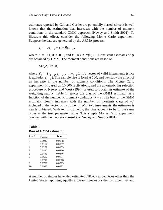
where is a vector of valid instruments (sincit excludes ). The sample size is fixed at 100, and we study the effecan increase in the number of moment conditions. The Monte Caexperiment is based on 10,000 replications, and the automatic lag seleprocedure of Newey and West (1994) is used to obtain an estimate oweighting matrix. Table 1 reports the bias of the GMM estimator asfunction of the number of moment conditions, . The bias of the GMestimator clearly increases with the number of moments (lags ofincluded in the vector of instruments. With two instruments, the estimatonearly unbiased. With ten instruments, the bias appears to be of theorder as the true parameter value. This simple Monte Carlo experimconcurs with the theoretical results of Newey and Smith (2001).

A number of studies have also estimated NKPCs in countries other thanUnited States, applying equally arbitrary choices for the instrument set

Table 1Bias of GMM estimator

k – 2 bias

2 0.0942 –0.00583 0.1157 0.01574 0.1209 0.01095 0.1410 0.04106 0.1446 0.04467 0.1607 0.06078 0.1716 0.07169 0.1799 0.079910 0.1932 0.0932

yt ρyt 1– εt θεt 1–+ +=

ρ 0.1 θ, 0.5= = εt i.i.d. N 0 1,( )∼ ρ

E εtZt( ) 0=

Zt yt 2– yt 3– . . . yt k–, , ,( )′=yt 1–

k 2–yt

ρGMM


ors.andand

dardhe

ntal

etingnt, itr thece oferent.ostsingthehen

hters iscon-

ed byex-

who

ationts areare in

the number of lags used in the construction of Newey-West standard err6

See, for example, Batini, Jackson, and Nickell (2002); Galí, Gertler,López-Salido (2001a); Gagnon and Khan (2001); and BalakrishnanLópez-Salido (2002).

To appreciate the relative importance of these choices within a stanGMM context, let and consider the reduced form under tconstraint :

, (11)

where . For a fixed value of, the parameter can be consistently estimated by instrume

variables, using lagged values of real marginal cost datedt and earlier.

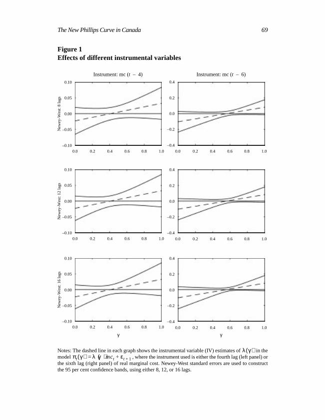
Using the same data set7 as Galí and Gertler (1999), Figure 1 shows theffects of different instruments and those of various lags in construcNewey-West estimates of the standard deviation. For a given instrumeappears that there is little effect whether 8, 12, or 16 lags are used foNewey-West standard errors. On the other hand, it is clear that the choiinstrument is crucial, especially at the upper end of the interval [0,1], whthe forward-looking component in the New Phillips curve is more importaWhen the sixth lag of marginal cost is used as the instrument, marginal ctend to appear marginally significant for some values of the forward-lookcomponent parameter near 0.7, while it is clearly insignificant whenfourth lag is used as the instrument. Note also the increased precision wthe fourth lag is used as the instrument as reflected by the relatively tigconfidence bands. The difference in the width of the confidence bandexpected, since the more recent lags are more strongly correlated withtemporaneous marginal cost and hence are better instruments.

Overall, these results cast doubt on the robustness of the results reportGalí and Gertler (1999) and on the significance of marginal costs inplaining U.S. inflation.

6. A few notable exceptions are Jondeau and Le Bihan (2001) and Lindé (2001)consider full information maximum likelihood approaches.7. The data are quarterly for the United States over the period 1960Q1–1997Q4. Inflis the annualized change in the logarithm of the GDP deflator, and real marginal cosmeasured as deviations from the sample mean of the logarithm of labour income shthe non-farm business sector.

γ γ f=γ f γb+ 1=

πt γ( ) λ γ( )mct εt 1++=

πt γ( ) πt πt 1–– γ πt 1+ πt 1––( )–=γ 0 1,[ ]∈ λ γ( )


Figure 1Effects of different instrumental variables

Notes: The dashed line in each graph shows the instrumental variable (IV) estimates of in themodel , where the instrument used is either the fourth lag (left panel) orthe sixth lag (right panel) of real marginal cost. Newey-West standard errors are used to constructthe 95 per cent confidence bands, using either 8, 12, or 16 lags.

λ γ( )πt γ( ) λ γ( )mct εt 1++=

0.4

0.2

0.0

–0.2

–0.4

0.0 0.2 0.4 0.6 0.8 1.0

0.10

0.05

0.00

–0.05

–0.10

Instrument: mc (t – 6)

New

ey-W

est:

8 la

gs

Instrument: mc (t – 4)

0.0 0.2 0.4 0.6 0.8 1.0

0.10

0.05

0.00

–0.05

–0.10

New

ey-W

est:

12 la

gs

0.0 0.2 0.4 0.6 0.8 1.0

0.10

0.05

0.00

–0.05

–0.10

New

ey-W

est:

16 la

gs

0.0 0.2 0.4 0.6 0.8 1.0

γ

0.4

0.2

0.0

–0.2

–0.4

0.0 0.2 0.4 0.6 0.8 1.0

0.4

0.2

0.0

–0.2

–0.4

0.0 0.2 0.4 0.6 0.8 1.0

γ


thenal

the

theGalí,sed

e thevalueinalrtler,atinges,ncateizethe

cted,case

der

2.2 Closed-form estimation à la Rudd-Whelan

As shown in Galí and Gertler (1999), the hybrid Phillips curve hasfollowing closed form, conditional on the expected path of real margicost:

, (12)

where and are, respectively, the stable and unstable roots ofhybrid Phillips curve given by:

, . (13)

An alternative to the standard GMM approach is to directly estimateclosed-form representation, as done in Rudd and Whelan (2001) andGertler, and López-Salido (2001a). Under rational expectations, the cloform defines the following orthogonality conditions:

, (14)

where is a vector of instrumental variables.

With this approach, it is necessary to use a truncated sum to approximatinfinite discounted sum of real marginal costs. Based on an assumedfor the discount factor , Rudd and Whelan use 12 leads of real margcost to construct the discounted stream of real marginal costs. Galí, Geand López-Salido, on the other hand, use 16 leads and differ by estimthe discount factor instead of fixing its value arbitrarily. In both cashowever, there is loss of degrees of freedom because of the need to truthe sum, which can be important given the relatively small sample s(typically about 30 years of quarterly data). Furthermore, given the waymeasure of the discounted stream of future marginal cost is construthere is a generated regressor problem. To see this, consider the limitingof pure forward-looking behaviour. In that case, the closed form, unrational expectations, becomes

, (15)

πt δ1πt 1–λ

δ2γ f----------- δ2

k–Et mct k+[ ]

k 0=

∞

∑+=

δ1 δ2

δ1

1 1 4γbγ f––

2γ f-------------------------------------= δ2

1 1 4γbγ f–+

2γ f-------------------------------------=

Et πt δ1πt 1––λ

δ2γ f----------- δ2mct k+

k 0=

∞

∑–

Zt 0=

Zt

β

πt λ βkmct k+ ut 1++

k 0=

∞

∑=


rror

inis

f theesenttedents

1986;alí,pt is

llynfi-s aomchyn).ppearualsed onhefor

icaled byduref the

-of-the

r ofiation

as

where the new error term, , is related to the original expectational eterm, , by

, (16)

and from which the generated regressor problem is apparent. Sinceequation (16) is serially correlated (into to the indefinite future), itessential that the efficiency of the GMM estimator and the consistency oassociated standard errors be evaluated. Clearly, this problem is also prin the hybrid Phillips curve. Estimation in the presence of generaregressors leads, in general, to inefficient estimates that require adjustmto obtain consistent estimates of their standard errors (see Pagan 1984,Murphy and Topel 1985; and McAleer and McKenzie 1991a, b). GGertler, and López-Salido (2001b) recognize this problem, but no attemmade to evaluate it.

Another problem associated with the closed form is that it involves locaalmost unidentified (LAU) parameters such that use of Wald-type codence intervals is invalid. The problem here is that the ratio hadiscontinuity at every point of the parameter space where . FrDufour (1997), it is then known that one can find a value of this ratio suthat the distribution of the Wald statistic will deviate arbitrarily from an“approximating distribution” (such as the standard normal distributioThis suggests that Wald-type inference on structural parameters that ain NKPC models in ratio form is, in general, an issue for any of the usestimation approaches. Other techniques, such as confidence sets bathe inversion of likelihood ratio tests, would yield valid inference on tLAU structural parameters. Note that Wald-type inference remains validthe “non-LAU” reduced-form parameters.

2.3 Estimation strategy

Our estimation strategy differs in three important ways from other empirstudies of the NKPC. First, we use bias-corrected estimators as proposNewey and Smith (2001). Second, an automatic lag-selection proceproposed by Newey and West (1994) is adopted to compute estimates ovariance-covariance matrix of the moment conditions.

As shown by several studies, the small sample properties of methodmoments estimators depends crucially on the number of lags used incomputation of this variance-covariance matrix. Moreover, our estimatothe variance-covariance matrix uses the sample moments in mean devin order to increase the power of the overidentifying restrictions test

ut 1+εt 1+

ut 1+ εt 1+ γ f πt 1+ λ βkmct k+

k 1=

∞

∑–+=

ut 1+

λ δ2γ f( )⁄γ f 0=


rlyfoundacksearn thenal

stepronas

the

ase of

ul-

ionalthe

tlerrid

tiontheent

ples,ith

suggested by Hall (2000). A more powerful specification test is cleadesirable, since it addresses the issues raised by Dotsey (2002) whothat the conventional specification test used in Galí and Gertler (1999) lpower. Third, an alternative estimator is used for the non-linspecification. This estimator has the advantage that it does not depend onormalization of the moment conditions, in contrast to the conventioGMM estimator.

We begin by presenting an alternative estimator to the conventional two-GMM estimator: the CUE, introduced by Hansen, Heaton, and Ya(1996). We then present bias-corrected linear IV, GMM, and CUE,proposed by Newey and Smith (2001).

The optimal two-step GMM estimator of Hansen (1982) based onmoment condition

is defined as

,

where is a first-step estimator usually obtained with the identity matrixweighting matrix, and where is a consistent estimator of the inversthe variance-covariance matrix of the moments conditions.

The CUE is analogous to GMM, except that the objective function is simtaneously minimized over and . This estimator is given by

.

This estimator has important advantages compared with the conventtwo-step estimator. First, unlike GMM, the estimator does not depend onnormalization of the moment conditions. As shown by Galí and Ger(1999), the results obtained for the New Phillips curve and the hybversion depend on the normalization adopted for the GMM estimaprocedure. Second, Newey and Smith (2001) have shown thatasymptotic bias of CUE does not increase with the number of momconditions. Hansen, Heaton, and Yaron (1996) show that in small samthe CUE has smaller bias for IV estimators of asset-pricing models wseveral overidentifying restrictions compared with that of GMM.

E g zt β0,( )[ ] 0=

β minβ B∈

1T---arg= g zt β,( )'Ω β( ) 1– 1

T--- g zt β,( )

t 1=

T

∑t 1=

T

∑

βΩ 1–

β Ω β( )

β minβ B∈

1T---arg= g zt β,( )'Ω β( ) 1– 1

T--- g zt β,( )

t 1=

T

∑t 1=

T

∑


, the001)sed

asticnd

isom

ods,

hisusing

en-.,

ure toirst,

there of

asless

f theateder tohatn bexes

Several approaches exist to correct for biases, including the jackknifebootstrap, subsampling, and analytical methods. Newey and Smith (2proposed an analytical bias correction for GMM and CUE estimators baon asymptotic bias formulas. Those formulas are derived from a stochexpansion to study higher than order properties of GMM aGeneralized Empirical Likelihood estimators. The bias-corrected CUEused for estimation of the non-linear specification. The bias formulas frNewey and Smith (2001) are adapted to a dynamic context.8 This analyticalbias correction is much simpler computationally than resampling methespecially in non-linear models.

3 Measuring the Labour Share with Canadian Data

The labour share is given by:

labour share , (17)

where is nominal labour income and is nominal output. From tbasic definition, several measures of labour share can be constructedavailable Canadian data.

A natural measure of the labour share is simply the ratio of total compsation of employees in the economy divided by the national income, i.e

lshare = wages and salaries/total GDP.

There are, however, some conceptual issues with the appropriate measuse in order to be consistent with the model’s theoretical framework. Fthe measure should be net of indirect taxes, since these accrue togovernment and do not constitute compensation to employees. A measulabour share adjusted for the effects of taxes is then constructedequation (17), but now the denominator is total GDP less indirect taxessubsidies on factors of production and on products.

Next, an adjustment should be made to account for the remuneration oself-employed. Given available data, the income of non-farm unincorporbusinesses can be added to the numerator of equation (17) in ordaccount for that part of the remuneration of the self-employed tconstitutes a return to labour rather than to capital. These two effects caaccounted for jointly, yielding a measure of labour share adjusted for taand self-employment.

8. Detailed derivations of the formulas are presented in Guay and Luger (2002).

1 T⁄

WNPY---------=

WN PY


usingnts,actorn be, andvel

then bepplybe

This

P

n inple

m its

bourss-t the

the

gs oftion(topted

y thewithco-ion isalsothe

s andelf-the

are

The first three measures of labour share just described are constructedincome-based GDP from the National Income and Expenditure Accouwhich is measured at market prices. Alternatively, measures based on fcosts can be considered in determining the labour share. These caconstructed by using the wages and salaries disaggregated by industrythe GDP at factor cost also at the industry level. By using industry-ledata, sectors where the theory does not apply can be excluded frommeasures of the labour share. For example, the public sector caexcluded, since the concepts of labour and capital shares arguably aonly to the market sector of the economy. The farm sector can alsoexcluded because of the very large subsidies that farmers receive.preferred measure is then constructed as

lsharenfb = (all industries, wages and salaries – farm wages andsalaries – public wages and salaries)/(all industries GD– farm GDP – public GDP).

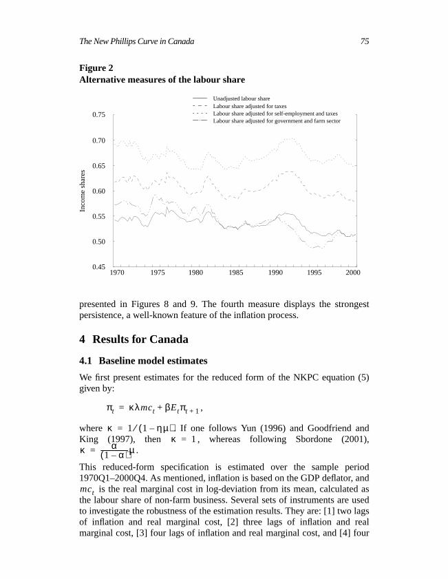
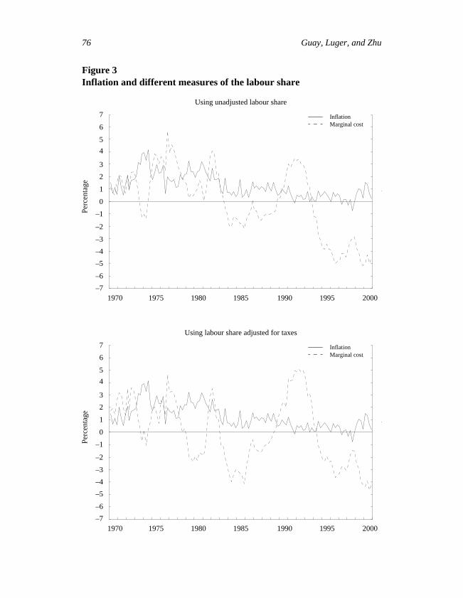
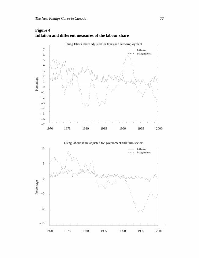
The levels of the different measures of the labour share are showFigure 2, where they seem to move in a similar fashion over the samperiod. Figures 3 and 4 show each measure in percentage deviation fromean, together with the inflation series (based on the GDP deflator).

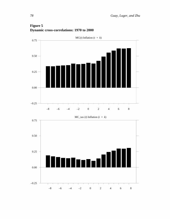
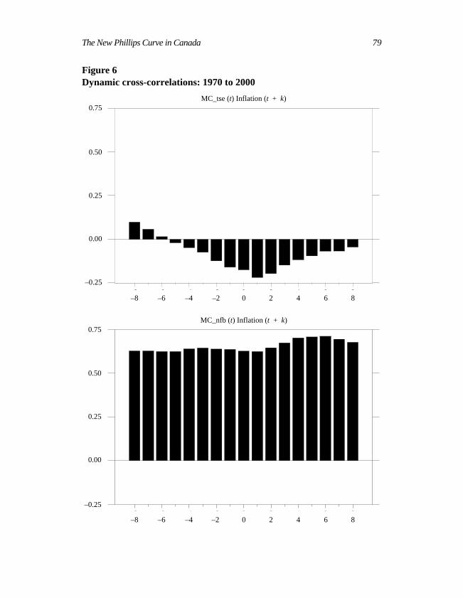
It becomes clear from these figures that the various measures of the lashare have very different relationships to inflation. Dynamic crocorrelations are presented in Figures 5 and 6, where it is obvious thafourth measure described above is potentially the most promising asexplanatory variable for Canadian inflation.

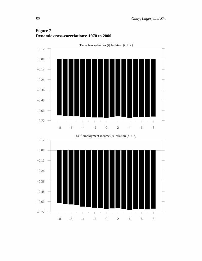
Note how the third measure co-moves negatively with most leads and lainflation. Figure 7 shows the dynamic cross-correlations between inflaand taxes less subsidies on factors of production and on productspanel), and between inflation and income of non-farm unincorporabusinesses (bottom panel).

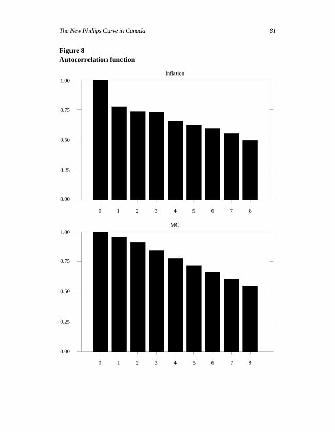
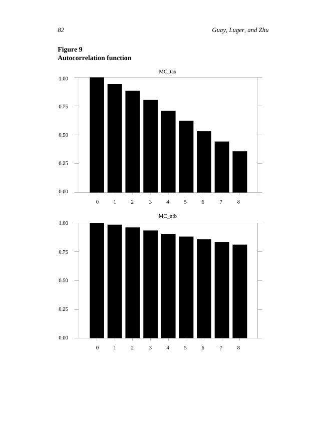
The strong negative co-movements seen in these figures explain whthird measure adjusted for taxes and self-employment is inconsistentthe new Phillips curve. One possible explanation for the negativemovement between taxes (less subsidies) and leads and lags of inflatthat the period of high oil prices in the 1970s and early 1980s wasaccompanied by high subsidies on imported oil. On the other hand,negative co-movements between income of the self-employed and leadlags of inflation might simply be due to the substantial upward trend in semployment vis-à-vis the downward movements in inflation. Finally,autocorrelation functions of the different measures of the labour share


gest

(5)

d),

riodandasusedlagsalur

Figure 2Alternative measures of the labour share

1970 1975 1980 1985 1990 1995 20000.45

0.50

0.55

0.60

0.65

0.70

0.75

0.45

0.50

0.55

0.60

0.65

0.70

0.75

unadjusted labour sharelabour share adjusted for taxeslabour share adjusted for self−employment and taxeslabour share adjusted for government and farm sector

Inco

me

Sha

res

Unadjusted labour shareLabour share adjusted for taxesLabour share adjusted for self-employment and taxesLabour share adjusted for government and farm sector

0.75

0.70

0.65

0.60

0.55

0.50

0.45

Inco

me

shar

es

1970 1975 1980 1985 1990 1995 2000

presented in Figures 8 and 9. The fourth measure displays the stronpersistence, a well-known feature of the inflation process.

4 Results for Canada

4.1 Baseline model estimates

We first present estimates for the reduced form of the NKPC equationgiven by:

,

where . If one follows Yun (1996) and Goodfriend anKing (1997), then , whereas following Sbordone (2001

.

This reduced-form specification is estimated over the sample pe1970Q1–2000Q4. As mentioned, inflation is based on the GDP deflator,

is the real marginal cost in log-deviation from its mean, calculatedthe labour share of non-farm business. Several sets of instruments areto investigate the robustness of the estimation results. They are: [1] twoof inflation and real marginal cost, [2] three lags of inflation and remarginal cost, [3] four lags of inflation and real marginal cost, and [4] fo

πt κλmct βEtπt 1++=

κ 1 1 ηµ–( )⁄=κ 1=

κ α1 α–( )-----------------µ=

mct


Figure 3Inflation and different measures of the labour share

1970 1975 1980 1985 1990 1995 2000−7

−6

−5

−4

−3

−2

−1

0

1

2

3

4

5

6

7

−7

−6

−5

−4

−3

−2

−1

0

1

2

3

4

5

6

7

InflationMarginal Cost

Using Unadjusted Labour Share

1970 1975 1980 1985 1990 1995 2000−7

−6

−5

−4

−3

−2

−1

0

1

2

3

4

5

6

7

−7

−6

−5

−4

−3

−2

−1

0

1

2

3

4

5

6

7


Using Labour Share Adjusted for Taxes

7

6

5

4

3

2

1

0

–1

–2

–3

–4

–5

–6

–7

Per

cent

age

1970 1975 1980 1985 1990 1995 2000

Using unadjusted labour share

InflationMarginal cost

7

6

5

4

3

2

1

0

–1

–2

–3

–4

–5

–6

–7

Per

cent

age

1970 1975 1980 1985 1990 1995 2000

Using labour share adjusted for taxes



Figure 4Inflation and different measures of the labour share

1970 1975 1980 1985 1990 1995 2000−7

−6

−5

−4

−3

−2

−1

0

1

2

3

4

5

6

7

−7

−6

−5

−4

−3

−2

−1

0

1

2

3

4

5

6

7


g j p yP

er c

en

t

1970 1975 1980 1985 1990 1995 2000−15

−10

−5

0

5

10

−15

−10

−5

0

5

10


Using Labour Share Adjusted for Government and Farm Sectors

Pe

r ce

nt

7

6

5

4

3

2

1

0

–1

–2

–3

–4

–5

–6

–71970 1975 1980 1985 1990 1995 2000

Using labour share adjusted for taxes and self-employment


10

5

0

–5

–10

–15

1970 1975 1980 1985 1990 1995 2000

Using labour share adjusted for government and farm sectors


Per

cent

age

Per

cent

age


Figure 5Dynamic cross-correlations: 1970 to 2000

MC(t) Inflation(t+k)

-8 -6 -4 -2 0 2 4 6 8-0.25

0.00

0.25

0.50

0.75

MC_tax(t) Inflation(t+k)

-8 -6 -4 -2 0 2 4 6 8-0.25

0.00

0.25

0.50

0.75

0.75

0.50

0.25

0.00

–0.25

MC(t) Inflation (t + k)

86420–2–4–6–8

0.75

0.50

0.25

0.00

–0.25

MC_tax (t) Inflation (t + k)

86420–2–4–6–8



MC_tse(t) Inflation(t+k)

-8 -6 -4 -2 0 2 4 6 8-0.25

0.00

0.25

0.50

0.75

MC_nfb(t) Inflation(t+k)

-8 -6 -4 -2 0 2 4 6 8-0.25

0.00

0.25

0.50

0.75

0.75

0.50

0.25

0.00

–0.25

MC_tse (t) Inflation (t + k)

86420–2–4–6–8

0.75

0.50

0.25

0.00

–0.25

MC_nfb (t) Inflation (t + k)

86420–2–4–6–8



Taxes less Subsidies(t) Inflation(t+k)

-8 -6 -4 -2 0 2 4 6 8-0.72

-0.60

-0.48

-0.36

-0.24

-0.12

0.00

0.12

Self-employment Income(t) Inflation(t+k)

-8 -6 -4 -2 0 2 4 6 8-0.72

-0.60

-0.48

-0.36

-0.24

-0.12

0.00

0.12

0.12

–0.12

–0.24

–0.48

–0.72

Taxes less subsidies (t) Inflation (t + k)

86420–2–4–6–8

0.00

–0.36

–0.60

Self-employment income (t) Inflation (t + k)

86420–2–4–6–8

0.12

–0.12

–0.24

–0.48

–0.72

0.00

–0.36

–0.60


Figure 8Autocorrelation function

Inflation

0 1 2 3 4 5 6 7 80.00

0.25

0.50

0.75

1.00

MC

0 1 2 3 4 5 6 7 80.00

0.25

0.50

0.75

1.00

1.00

0.75

0.50

0.25

0.00

Inflation

876543210

1.00

0.75

0.50

0.25

0.00

MC

876543210


Figure 9Autocorrelation function

MC_tax

0 1 2 3 4 5 6 7 80.00

0.25

0.50

0.75

1.00

MC_nfb

0 1 2 3 4 5 6 7 80.00

0.25

0.50

0.75

1.00

1.00

0.75

0.50

0.25

0.00

MC_tax

876543210

1.00

0.75

0.50

0.25

0.00

876543210

MC_nfb


atedure-

thed asdardunit

hesisby athesualtputp istput.lityreal

IVined

istentn tod bytionportsan

t isform, itsthat

t onhreeeatertedal

ande of

lags of inflation, real marginal cost, and nominal wages. Instruments dand earlier are used to mitigate possible correlations with the meas

ment error of real marginal cost.

We depart from earlier studies by excluding output-gap measures frominstrument sets. Two measures of output gap are usually retaineinstruments. One is based on quadratically detrended output. With stanunit-root tests (such as the Augmented Dickey-Fuller), the presence of aroot in Canadian output cannot be rejected. Under the maintained hypotof a unit root, quadratically detrended output is then also characterizedunit root. Unfortunately, the asymptotic properties of IV estimators inpresence of non-stationary instruments are not known. As a result, uinference procedures are likely to be invalid. The other measure of ougap usually used is based on the Hodrick-Prescott filter. The output gathen a combination of lags, leads, and contemporaneous values of ouSuch measures of the output gap violate the basic GMM orthogonaconditions and are likely to be correlated with the measurement error ofmarginal cost.

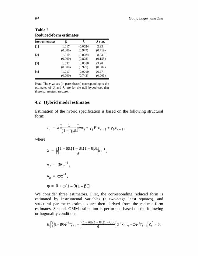
The GMM estimator for this linear specification corresponds to theestimator (two-stage least squares), which we correct for bias, as explaabove. We also use a heteroscedasticity and autocorrelation-consmatrix estimator for the sample moments in deviations from the meaincrease the power of the overidentifying restrictions test, as suggesteHall (2000) and Bonnal and Renault (2001). The automatic lags selecprocedure proposed by Newey and West (1994) is adopted. Table 2 rethe results for . This value is proposed by Gagnon and Kh(2001) for Canada following the assumptions in Sbordone (2001). Iimportant to understand that the inference results based on the reduceddo not depend on . While the scaling of the parameter depends onstatistical significance does not, since the value of is a fixed constantcancels out from thet-statistic.

The results are not encouraging for the NKPC. The slope coefficienmarginal cost is never significant whatever the set of instruments. For tcases, the coefficient has the wrong sign, and the discount factor is grthan one in all cases. Finally, the overidentifying restrictions are rejecwith the instrument sets, which include four lags of inflation and remarginal cost. It appears that the New Phillips curve is misspecified,richer dynamics would seem necessary to capture the persistencCanadian inflation.

t 1–

κ 0.13=

κ λ κκ


ral

isand

forming

4.2 Hybrid model estimates

Estimation of the hybrid specification is based on the following structuform:

,

where

,

,

,

.

We consider three estimators. First, the corresponding reduced formestimated by instrumental variables (a two-stage least squares),structural parameter estimates are then derived from the reduced-estimates. Second, GMM estimation is performed based on the followorthogonality conditions:

.

Table 2Reduced-form estimates

Instrument set J-stat.

[1] 1.017(0.000)

–0.0024(0.947)

2.83(0.419)

[2] 1.010(0.000)

–0.0084(0.803)

8.03(0.155)

[3] 1.037(0.000)

0.0010(0.977)

23.20(0.002)

[4] 1.011(0.000)

–0.0010(0.742)

26.97(0.005)

Note: Thep-values (in parentheses) corresponding to theestimates of and are for the null hypotheses thatthese parameters are zero.

β λ

β λ

πt λ 11 ηµ–( )

--------------------- mct γ f Etπt 1+ γbπt 1–+ +=

λ 1 ω–( ) 1 θ–( ) 1 θβ–( )θ

-------------------------------------------------------- φ 1–

=

γ f βθφ 1–=

γb ωφ 1–=

φ θ ω 1 θ 1 β–( )–[ ]+=

Et πt βθφ 1– πt 1+–1 ω–( ) 1 θ–( ) 1 θβ–( )

θ--------------------------------------------------------

φ 1– κmct– ωφ 1– πt 1–– Zt 0=


nsther

ion.of

turalthe.

ard-nt.is

eci-of

he. Thees.e

t thetesandin

ith

yees

byded.

t the

hours

Note that GMM estimation results from the same orthogonality conditiodepend on the chosen normalization (Galí and Gertler 1999). On the ohand, the CUE, by construction, is invariant to the choice of normalizatFollowing Newey and Smith (2001), analytical bias-corrected versionsthese three estimators can be computed.

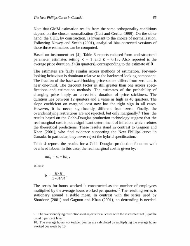
Based on instrument set [4], Table 3 reports reduced-form and strucparameter estimates setting and . Also reported isaverage price duration,D (in quarters), corresponding to the estimate of

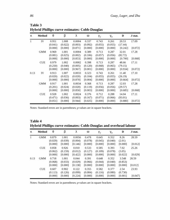
The estimates are fairly similar across methods of estimation. Forwlooking behaviour is dominant relative to the backward-looking componeThe fraction of the backward-looking price-setters differs from zero andnear one-third. The discount factor is still greater than one across spfications and estimation methods. The estimates of the probabilitychanging price imply an unrealistic duration of price stickiness. Tduration lies between 12 quarters and a value as high as 48 quartersslope coefficient on marginal cost now has the right sign in all casHowever, it is never significantly different from zero. Finally, thoveridentifying restrictions are not rejected, but only marginally.9 Thus, theresults based on the Cobb-Douglas production technology suggest thareal marginal cost is not a significant determinant of inflation, which refuthe theoretical predictions. These results stand in contrast to GagnonKhan (2001), who find evidence supporting the New Phillips curveCanada. In particular, they never reject the hybrid specification.

Table 4 reports the results for a Cobb-Douglas production function woverhead labour. In this case, the real marginal cost is given by:

,

where

.

The series for hours worked is constructed as the number of emplomultiplied by the average hours worked per quarter.10 The resulting series isstationary around a stable mean. In contrast with the series usedSbordone (2001) and Gagnon and Khan (2001), no detrending is nee

9. The overidentifying restrictions test rejects for all cases with the instrument set [3] ausual 5 per cent level.10. The average hours worked per quarter are calculated by multiplying the averageworked per week by 13.

κ 1= κ 0.13=θ

mct st bht+=

bH H⁄

1 H H⁄–----------------------=


Table 3Hybrid Phillips curve estimates: Cobb-Douglas

Method D J-stat.

1 IV 0.951(0.041)[0.000]

1.008(0.022)[0.000]

0.0004(0.003)[0.871]

0.337(0.092)[0.000]

0.743(0.055)[0.000]

0.261(0.055)[0.000]

20.53(17.44)[0.242]

17.09

[0.072]

GMM 0.969(0.081)[0.000]

1.001(0.025)[0.000]

0.0004(0.002)[0.853]

0.389(0.106)[0.000]

0.713(0.057)[0.000]

0.287(0.056)[0.000]

32.01(82.72)[0.700]

17.28

[0.068]

CUE 0.979(0.250)[0.000]

1.002(0.040)[0.000]

0.0002(0.005)[0.967]

0.398(0.120)[0.001]

0.713(0.068)[0.000]

0.287(0.065)[0.000]

48.66(79.15)[0.934]

17.11

[0.072]

0.13 IV 0.913(0.020)[0.000]

1.007(0.022)[0.000]

0.0033(0.020)[0.870]

0.323(0.104)[0.004]

0.743(0.055)[0.000]

0.261(0.055)[0.000]

11.40(26.19)[0.664]

17.10

[0.072]

GMM 0.917(0.201)[0.000]

1.001(0.024)[0.000]

0.0034(0.020)[0.850]

0.368(0.119)[0.003]

0.713(0.056)[0.000]

0.287(0.056)[0.000]

12.03(29.57)[0.685]

17.28

[0.068]

CUE 0.928(0.471)[0.051]

1.002(0.036)[0.000]

0.0024(0.003)[0.944]

0.376(0.167)[0.025]

0.712(0.071)[0.000]

0.288(0.066)[0.000]

14.04(93.01)[0.880]

17.11

[0.072]

Notes: Standard errors are in parentheses;p-values are in square brackets.

Table 4Hybrid Phillips curve estimates: Cobb-Douglas and overhead labour

Method D J-stat.

1 GMM 0.879(0.029)[0.000]

1.001(0.039)[0.000]

0.0056(0.004)[0.146]

0.478(0.078)[0.000]

0.645(0.045)[0.000]

0.352(0.040)[0.000]

8.26(2.01)[0.000]

28.59

[0.012]

CUE 0.858(0.062)[0.000]

0.926(0.159)[0.000]

0.010(0.012)[0.422]

0.533(0.127)[0.000]

0.585(0.109)[0.000]

0.393(0.078)[0.000]

7.02(3.05)[0.022]

25.26

[0.029]

0.13 GMM 0.718(0.068)[0.000]

1.001(0.033)[0.000]

0.044(0.029)[0.138]

0.391(0.066)[0.000]

0.648(0.044)[0.000]

0.352(0.040)[0.000]

3.548(0.853)[0.000]

28.59

[0.012]

CUE 0.607(0.113)[0.000]

0.902(0.126)[0.000]

0.122(0.099)[0.224]

0.355(0.084)[0.000]

0.582(0.116)[0.000]

0.377(0.080)[0.000]

2.54(0.730)[0.001]

23.93

[0.047]


κ θ β λ ω γ f γb

κ θ β λ ω γ f γb


four

eandw

ible,asebutfornt,

t ofe andodeltionrtednot

tion

ostare

thethe

verhe

be int it isands off thes of

ifica-ativeying

Finally, the instrument set corresponds to the fourth one augmented bylags of hours worked.

We first tried to estimate the parameterb. Unfortunately, the estimates wernever significant. Instead, we report the results obtained with GMMCUE for a value ofb, calibrated as in other empirical studies of the NePhillips curve. Following Rotemberg and Woodford (1999),b is calibratedto 0.4. The estimates of price-stickiness duration are now more plausespecially for . The discount factor is now less than one in the cof estimation by CUE. The forward-looking component still dominates,now the fraction of backward-looking price-setters is more important

. Here again, the slope coefficient on marginal is never significaand the specification is rejected in all cases.

We also tried to estimate the specification including the adjustment coslabour based on equation (6). Labour is measured as explained abovthe instrument set is the same as for estimation of the previous mspecification. The parameter was never significant across estimamethods. We then calibrated this parameter following the estimates repoby Ambler, Guay, and Phaneuf (1999). The estimation results weresignificantly different from the ones based on a Cobb-Douglas producfunction without adjustment cost.

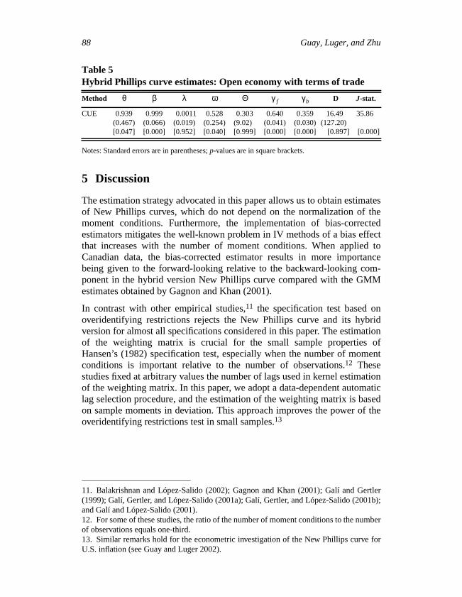
4.3 Open economy

We proceed to estimate the hybrid specification with real marginal caugmented by the terms of trade as in equation (7). The terms of tradecalculated as the logarithm of the import price minus the logarithm ofdomestic GDP deflator. Instrument set [4] augmented with four lags ofterms of trade is used.

In this case as well, the relative coefficient to the terms of trade is nesignificant. Table 5 reports estimates obtained with CUE for . Tparameter of openness, , has a point estimate, which seems toaccordance with the degree of openness of the Canadian economy, bunot statistically significant. The other results are similar to previous onesagain the specification is decisively rejected. The addition of the termtrade in the instrument set results in an important increase in the value ooveridentifying restrictions test statistic. This suggests that the termtrade could be an important explanatory variable for Canadian inflation.

The results are similar when we replace the terms of trade in the spection of real marginal cost by the real exchange rate. The parameter relto the real exchange rate is estimated imprecisely, and the overidentifrestrictions test clearly rejects the model in all cases.

κ 0.13=

κ 1=

φ

κ 0.13=Θ


atesthetedect

toancem-M

nridtionofent

tionaticsed

f the

rtler1b);

mber

for

Table 5Hybrid Phillips curve estimates: Open economy with terms of trade

Method D J-stat.

CUE 0.939(0.467)[0.047]

0.999(0.066)[0.000]

0.0011(0.019)[0.952]

0.528(0.254)[0.040]

0.303(9.02)[0.999]

0.640(0.041)[0.000]

0.359(0.030)[0.000]

16.49(127.20)

[0.897]

35.86

[0.000]


θ β λ ω Θ γ f γb

5 Discussion

The estimation strategy advocated in this paper allows us to obtain estimof New Phillips curves, which do not depend on the normalization ofmoment conditions. Furthermore, the implementation of bias-correcestimators mitigates the well-known problem in IV methods of a bias effthat increases with the number of moment conditions. When appliedCanadian data, the bias-corrected estimator results in more importbeing given to the forward-looking relative to the backward-looking coponent in the hybrid version New Phillips curve compared with the GMestimates obtained by Gagnon and Khan (2001).

In contrast with other empirical studies,11 the specification test based ooveridentifying restrictions rejects the New Phillips curve and its hybversion for almost all specifications considered in this paper. The estimaof the weighting matrix is crucial for the small sample propertiesHansen’s (1982) specification test, especially when the number of momconditions is important relative to the number of observations.12 Thesestudies fixed at arbitrary values the number of lags used in kernel estimaof the weighting matrix. In this paper, we adopt a data-dependent automlag selection procedure, and the estimation of the weighting matrix is baon sample moments in deviation. This approach improves the power ooveridentifying restrictions test in small samples.13

11. Balakrishnan and López-Salido (2002); Gagnon and Khan (2001); Galí and Ge(1999); Galí, Gertler, and López-Salido (2001a); Galí, Gertler, and López-Salido (200and Galí and López-Salido (2001).12. For some of these studies, the ratio of the number of moment conditions to the nuof observations equals one-third.13. Similar remarks hold for the econometric investigation of the New Phillips curveU.S. inflation (see Guay and Luger 2002).


estsd toates,rvedlipsstep

llipsnewturalbesed

isthat

pe of

lipsof the

Conclusions

The rejection of alternative specifications of the New Phillips curve suggthat a richer dynamic structure in the explanatory variables will be needecapture the dynamics of Canadian inflation. In the case of the United StKurmann (2002) also finds considerable uncertainty between the obsepersistent movements in inflation and what is predicted by a New Philcurve model. His results and those of this paper represent an importantback from the conclusions of previous authors who argue that New Phicurve models are a good representation of inflation dynamics. Theseresults suggest that, at the theoretical level, richer versions of the strucmodel from which the New Phillips curve is derived would need todeveloped. Mankiw and Reis (2002) proposed a “sticky-information”-baPhillips curve that can generate inflation dynamics similar to whatobserved in the data. However, assessing the empirical relevance ofmodel raises several other econometric issues that go beyond the scothis paper.14

14. Khan and Zhu (2002) report estimates of the “sticky-information”-based Philcurve. However, their inference method suffers from a generated regressor problemtype mentioned above.


allylessSIM

ts)

at006

of

AppendixData Description

When applicable, the final series is in quarterly frequency, seasonadjusted, at annual rates, and in millions (of dollars or persons), unotherwise indicated. The series codes are from Statistics Canada’s CANdatabase.

1. Total GDP deflator: constructed from the following series.

• Nominal GDP = V498086

• Constant dollar GDP = V1992259

• Chained dollar GDP = V1992067

2. Labour income share

• lshare = wages and salaries/total GDP = V498076/V498074

• lsharetax = wages and salaries/(total GDP – indirect taxes lesssubsidies on factors of production and on products)

= V498076/(V498074 – V1992216 – V1997473)

• lsharetse = (wages and salaries + income of non-farmunincorporated business)/(total GDP – indirect taxesless subsidies on factors of production and on produc

= (V498076 + V498081)/(V498074 – V1992216– V1997473)

• lsharenfb = (all industries wages and salaries – farm wages andsalaries – public wages and salaries)/(all industriesGDP – farm GDP – public GDP)

Note: lsharenfb is constructed from CANSIM Table 379–0006 (GDPfactor cost), 382–0001 (old table for wages and salaries), and 382–0(new table for wages and salaries).

3. Import prices: constructed from the following series.

• Nominal imports = V498106

• Constant dollar imports = V1992253

• Chained dollar imports = V1992063

4. Hours worked

• Average hours worked per week, all industries = LSA2050 (BankCanada series code)


5. Employment

• Total employment, 15 years old and above = D767608 andV2062811

• Private sector employment = total employment – V2066969

6. Population

• Population, 15 years old and above = D767284 and V2091030

7. Nominal exchange rates

• Canadian dollar/U.S. dollar closing rate = B3414 (monthlyfrequency, a quarter is the average of three months)


rrsité

w

n:

g

o

ric

w

.the

References

Ambler, S., A. Guay, and L. Phaneuf. 1999. “Wage Contracts and LaboAdjustment Costs as Endogenous Propagation Mechanisms.” Univedu Québec à Montréal. Manuscript.

Ambler, S., A. Kurmann, and A. Guay. 2002, “On Aggregation and the NePhillips Curve.” Université du Québec à Montréal. Manuscript.

Balakrishnan, R. and J.D. López-Salido. 2002. “Understanding UK Inflatiothe Role of Openness.” Bank of England Working Paper No. 164.

Batini, N., B. Jackson, and S. Nickell. 2002. “Inflation Dynamics and theLabour Share in the UK.” Bank of England External MPC UnitDiscussion Paper No. 2.

Bonnal, H. and E. Renault. 2001. “Minimal Chi-Square Estimation withConditional Moment Restrictions.” Manuscript.

Calvo, G. 1983. “Staggered Prices in a Utility-Maximizing Framework.”Journal of Monetary Economics 12 (3): 383–98.

Danthine, J.-P. and J.B. Donaldson. 2002. “A Note on NNS Models:Introducing Physical Capital; Avoiding Rationing.”Economics Letters77 (3): 433–37.

Dotsey, M. 2002. “Pitfalls in Interpreting Tests of Backward-Looking Pricinin New Keynesian Models.” Federal Reserve Bank of RichmondEconomic Quarterly 88 (1): 37–50.

Dufour, J.-M. 1997. “Some Impossibility Theorems in Econometrics withApplications to Structural and Dynamic Models.”Econometrica65 (6): 1365–87.

Gagnon, E. and H. Khan. 2001. “New Phillips Curve with AlternativeMarginal Cost Measures for Canada, the United States, and the EurArea.” Bank of Canada Working Paper No. 2001–25.

Galí, J. and M. Gertler. 1999. “Inflation Dynamics: A Structural EconometAnalysis.”Journal of Monetary Economics 44 (2): 195–222.

Galí, J., M. Gertler, and J.D. López-Salido. 2001a. “European InflationDynamics.”European Economic Review 45 (7): 1237–70.

———. 2001b. “Notes on Estimating the Closed Form of the Hybrid NePhillips Curve.” New York University. Manuscript.

Galí, J. and J.D. López-Salido. 2001. “A New Phillips Curve for Spain.”Manuscript.

Galí, J. and T. Monacelli. 2002. “Monetary Policy and Exchange RateVolatility in a Small Open Economy.” NBER Working Paper No. 8905

Goodfriend, M. and R. King. 1997. “The New Neoclassical Synthesis andRole of Monetary Policy.”NBER Macroeconomics Annual. Cambridge,Mass.: MIT Press.


f

of

psde

of

ng

h

s:pt.rs

t

ep

nd

ce

th

s.”

es

Guay A. and R. Luger. 2002. “The U.S. New Keynesian Phillips Curve:An Econometric Investigation.” Manuscript.

Hall, A.R. 2000. “Covariance Matrix Estimation and the Power of theOveridentifying Restrictions Test.”Econometrica 68 (6): 1517–28.

Hansen, L.P. 1982. “Large Sample Properties of Generalized Method oMoments Estimators.”Econometrica 50 (4): 1029–54.

Hansen, L.P., J. Heaton, and A. Yaron. 1996. “Finite-Sample PropertiesSome Alternative GMM Estimators.”Journal of Business and EconomicStatistics 14 (3): 262–80.

Jondeau, E. and H. Le Bihan. 2001. “Testing for a Forward-Looking PhilliCurve: Additional Evidence from European and U.S. Data.” Banque France Working Paper No. 86.

Khan, H. and Z. Zhu. 2002. “Estimates of the Sticky-Information PhillipsCurve for the United States, Canada, and the United Kingdom.” BankCanada Working Paper No. 2002–19.

Kurmann, A. 2002. “Quantifying the Uncertainty about a Forward-LookiNew Keynesian Pricing Model.” University of Virginia. Manuscript.

Lindé, J. 2001. “Estimating New-Keynesian Phillips Curves on Data witMeasurement Errors: A Full Information Maximum LikelihoodApproach.” Sveriges Riksbank Working Paper No. 129.

Mankiw, G.N. and R. Reis. 2001. “Sticky Information Versus Sticky PriceA Proposal to Replace the New Keynesian Phillips Curve.” Manuscri

McAleer, M. and C.R. McKenzie. 1991a. “When Are Two Step EstimatoEfficient?”Econometric Reviews 10 (2): 235–52.

———. 1991b. “Keynesian and New Classical Models of UnemploymenRevisited.”Economic Journal 101 (406): 359–81.

Murphy, K.M. and R.H. Topel. 1985. “Estimation and Inference in Two-StEconometric Models.”Journal of Business and Economics Statistics3 (4): 370–79.

Newey, W.K. and R.J. Smith. 2001. “Higher Order Properties of GMM aGeneralized Empirical Likelihood Estimators.” Manuscript.

Newey, W.K. and K.D. West. 1994. “Automatic Lag Selection in CovarianMatrix Estimation.”Review of Economic Studies 61 (4): 631–53.

Pagan, A. 1984. “Econometric Issues in the Analysis of Regressions wiGenerated Regressors.”International Economic Review 25 (1): 221–47.

———. 1986. “Two Stage and Related Estimators and Their ApplicationReview of Economic Studies 53 (4): 517–38.

Rotemberg, J.J. and M. Woodford. 1999. “The Cyclical Behavior of Pricand Costs.” InHandbook of Macroeconomics, Vol. 1B, edited byJ.B. Taylor and M. Woodford. North-Holland: Elsevier Science E.V.


ps
Rudd, J. and K. Whelan. 2001. “New Tests of the New-Keynesian PhilliCurve.” Federal Reserve Board Discussion Series No. 2001–30.
Sbordone, A. 2001. “Prices and Unit Labor Costs: A New Test of PriceStickiness.”Journal of Monetary Economics 49 (2): 265–92.

Taylor, J.B. 1980. “Aggregate Dynamics and Staggered Contracts.”Journalof Political Economy 88 (1): 1–23.

Yun, T. 1996. “Nominal Price Rigidity, Money Supply Endogeneity, andBusiness Cycles.”Journal of Monetary Economics 37 (2–3): 345–70.

Date post:	16-Jul-2018
Category:	Documents
Upload:	volien
View:	214 times
Download:	0 times

The New Phillips Curve in Canada - Bank of Canada€¦ · To obtain a Phillips curve relationship...

Documents