J.-M. Lemoine (1), S. Bourgogne (2), R.

Biancale (3), F. Reinquin (1)

1) CNES/GRGS, Toulouse, France

2) Géode & Cie, Toulouse, France /

Stellar Space Studies , Toulouse, France

3) GFZ, Oberpfaffenhofen, Germany

The new time-variable gravity field model for POD of altimetric satellites based on GRACE+SLR RL04 from CNES/GRGS

Introduction

Precise orbit determination is a key element in the overall accuracy of the altimetric measurements.

Since 2002, thanks to the GRACE (and GOCE) missions, we have now a very good knowledge of the Earth gravity field and its time evolution.

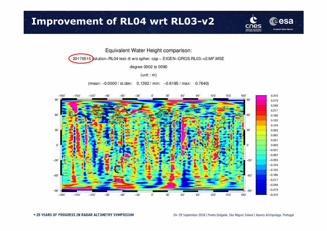
Based on 14 years of GRACE data (2002.5-2016.5), 3 years of GOCE data and 33 years of SLR data (1985-2018), the EIGEN-GRGS.RL04.MEAN-FIELD is the gravity model that is proposed for the GDR-F standards.

It contains a time-variable gravity (TVG) part until degree and order 90, and a static part coming from the model GOCE-DIR5 up to degree and order 300.

The TVG part is modeled for each year between August 2002 and June 2016 as an annual bias + slope + annual and semi-annual periodic components.

For the low degrees of the gravity field, the TVG part prior to August 2002will either :

Be modeled, for degree 2 only, by SLR data from January 1985 to July 2002

Or be modeled in a more ambitious way thanks to a “mascon” approach (see John Moyard’s presentation, following talk).

GRACE (L-1B “Version2” data)

● K-Band Range-Rate data (σapriori = .1 μm/s)

● GPS data (1-day arcs, σcode = 80 cm, σphase = 20 mm / 30s resolution)

● ACC and SCA data (KBR CoP coordinates solved once / day)

Data processing in the RL04 reprocessing(June – December 2017)

Physical parameters present in the normal equations

● Gravity spherical harmonic coefficients complete to degree

and order 90 (truncated to 30 for LAGEOS and 40 for GPS data)

● Ocean tides s. h. coefficients for 14 tidal waves with maximum

degree/order ≤ 30 (not used yet)

SLR

● Lageos1/2 data (10-day arcs, σapriori = 6 mm)

● Starlette/Stella data (5-day arcs, σapriori = 10 mm)

Gravity

Ocean tide

Atmosphere 3-D ECMWF ERA-interim pressure grids / 3 hrs

Ocean mass model TUGO (Legos) / 3 hrs

Atmospheric tides

3rd body Sun, Moon, 6 planets (DE405)

Solid Earth tides IERS Conventions 2010

Pole tides IERS Conventions 2010

Non gravitational Accelerometer data (+biases and scale factors)

SLR stations

GPS

HydrologyTaken into account by the a priori gravity field

Glacial Isostatic Adjustment

Dynamical models

Geometrical models

Other models

Models used:

EIGEN-GRGS.RL03-v2.MEAN-FIELD

FES2014 (Legos)

→ Not necessary because of the 3 hrs dealiasing time sampling

ITRF2014 coordinates

IGS Repro-2 orbits & clocks

From GRACE monthly solutions to mean gravity models

Using directly GRACE/GRACE-FO monthly solutions is not appropriate for POD

because of:

Data gaps in the GRACE time series (e.g. after 2011 and between GRACE and

GRACE-FO)

The problem of extrapolation before 2002 and after 2016

Mean models are now generated from time series

Fitting each series of monthly spherical harmonic coefficients by a set of 6

parameters :

Yearly bias and slope : piecewise linear function except in case of …

Jumps caused by big earthquakes (so far : Sumatra/2005.0,

Concepcion/2010.2 and Tohoku/2011.2)

Annual and semi-annual sine/cosine functions (with continuity

constraints at hinge epochs)

It means 750 000 coefficients for a 90x90 spherical harmonic model

RL04 mean model

Example for one spherical harmonic coefficient:

GRACE monthly

time series

Mean model with

bias, drift per year,

annual and semi-

annual periodic

terms per year

Large Earthquake

events

Mean model: from RL03-v2 to RL04

The new mean field updates the previous one over 2 years: mid-2014 to mid-2016.

Example for the C(2,0) spherical harmonic coefficient:

Small changes due to the

transition from RL03-v2 to

RL04

Important changes due to

the addition of 2 more

years

----- RL03-v2----- RL04

Update of the mean model from -v2 to -v3 Extrapolation vs. real data after 2 years: difference between mean-field –v2 and mean

field –v3 at mid-2016

Improvement of RL04 wrt RL03-v2

Noise assessment can be made in areas with no or very little mass variations: Sahara and Gobi deserts, East Antarctica, South and Equatorial Pacific

RL03/RL04 evaluation

Sahara desert: 2.2 Mkm2

South Pacific 6.7 Mkm2

East Antarctica: 3.6 Mkm2

Gobi desert: 1.6 Mkm2

Equatorial Pacific: 31.6 Mkm2

Noise assessment over the Sahara

The Sahara desert shows very little hydrological variations. We have delimited a

rectangular zone of 2.2 Mkm2 where almost no gravity variation is suspected

(except a small depletion of 1.3 mm/yr in South Libya).

It is hence well dedicated to control the quality of gravity field variation models.

The surface is first divided in 2 deg.*2 deg. blocs ( degree/order 90), then

averaged in blocs of larger size up to 20 deg.*20 deg. Drift and annual/semi-

annual variations are fitted a priori.

Different time-varying gravity models with various DDK filters (Kusche et al.) are

compared spectrally in this way from 100 km to 2200 km.

RL03

RL04

DDK6 TUG

DDK6 TUGOver 2006-2007

DDK5 TUG

DDK7 TUG

DDK6 CSR

Over 2003-2016

DDK6 CSR

RL04 time series

RL04 mean field

Noise assessment over “deserts”

Equatorial Pacific ocean

Gobi desert

East Antarctica

Sahara desert

Signal assessment by comparison to altimetry

RL04 time series RL04 mean field

ITSG16 / DDK5

(Caspian Sea)

Altimeter time series from Hydroweb (https://sso.theia-land.fr)

Signal assessment by comparison to altimetry(Caspian Sea)

CORRELATION SCALE FACTOR

RL0

4 t

ime

se

rie

s

RL0

4 m

ea

n f

ield

RL0

4 t

ime

se

rie

s

RL0

4 m

ea

n f

ield

Signal assessment by comparison to altimetry

15 / 13

(Black Sea)

CORRELATION SCALE FACTOR

Altimeter time

series from

Copernicus

(http://marine.cop

ernicus.eu).

Need for consistency

MEAN POLE MODEL and GRAVITY FIELD

• When using the C(2,1)/S(2,1) values of a gravity field model, one must adopt the

same mean pole convention as the one used for the computation of the model.

• CNES/GRGS is using the mean pole of the IERS2010 conventions. If the

conventions change for a linear mean pole, then the C(2,1)/S(2,1) coefficients of

the mean gravity model will have to be adapted to this new convention.

DEALIASING MODELS and GRAVITY FIELD

• The same goes for the dealiasing models : CNES uses 3-hour ERA-Interim &

TUGO models the same models should be used for POD

The new mean gravity field model based on CNES/GRGS RL04 is available for the

GRACE period (2002 – 2016)

Validation tests (noise and signal w.r.t. altimetry) show a good performance of this

RL04 mean field

Extrapolated periodic terms (before August 2002 and after May 2016) are based on

global fits of monthly coefficients over 14 years of GRACE data

It still needs to be completed before and after the GRACE period by additional data

coming from SLR data (and DORIS data ?) in order to follow the long-term evolution

of the lower degrees

Possibly an accurate modeling of only the degree 2 through SLR and DORIS data is

sufficient to achieve good POD performances

When doing POD one must ensure that the models used are not only “good” but

also consistent !!!

Conclusions and perspectives