1 The Norwegian Government Pension Fund’s potential for capturing illiquidity premiums Frank de Jong and Joost Driessen 1 Tilburg University February 2013 1 This report is written for the Norwegian Ministry of Finance. Both authors are affiliated with the Department of Finance, Tilburg University. Contact address: Warandelaan 2, PO Box 90153, 5000 LE Tilburg, Netherlands. Fax: +31 466 2875. Phone and email: Frank de Jong: +31 466 8040, [email protected]; Joost Driessen: +31 466 2324, [email protected]
Transcript
1
The Norwegian Government Pension Fund’s potential for
capturing illiquidity premiums
Frank de Jong and Joost Driessen1
Tilburg University
February 2013
1 This report is written for the Norwegian Ministry of Finance. Both authors are affiliated with the
Department of Finance, Tilburg University. Contact address: Warandelaan 2, PO Box 90153, 5000 LE
Tilburg, Netherlands. Fax: +31 466 2875. Phone and email: Frank de Jong: +31 466 8040,
The Norwegian ministry of finance has asked us to investigate the possibilities for the Government
Pension Fund Global (GPFG) to profit from liquidity premiums in illiquid investments. Can a large
investor with a long horizon, limited short term liquidity needs and high risk bearing capacity, such
as the GPFG, profit from these liquidity premiums? The ministry has asked a number of specific
questions.
The first set of questions is about the theoretical motivation for liquidity premiums. Under what
circumstances and for which types assets can one expect the presence of a liquidity premium? What
are the sources of illiquidity and do they matter for the magnitude of liquidity premiums?
The second set of questions concern the empirical evidence. In which asset classes is there a liquidity
premium? How large are these premiums? What are the potential obstacles to profit from these?
Historically, liquidity premiums in some markets seem to be high, but what is the recent evidence?
What is the impact of the dramatic changes in financial market structure (the move to fully
electronic trading, high frequency trading and increased competition between exchanges) over the
last decade?
A third set of questions are more specifically about the measures of liquidity. Theoretically, what
measure of liquidity should one use? And practically, does one need intraday transaction data to
estimate liquidity or are approximate measures based on daily data sufficient?
The final set of questions concerns the rebalancing towards the strategic investment portfolio. How
does illiquidity affect the timing and size of rebalancing trades? What is the trade-off between costs
of rebalancing trades and the costs of a suboptimal asset allocation? In this report, we focus on long-
term investment and rebalancing strategies. We do not investigate how investors can profit from
illiquidity by acting as a liquidity provider using intraday high-frequency trading.
In this report, we provide an extensive overview of the recent academic literature concerning these
questions. We do not strive for completeness of the review, although we think we cover the most
important work. Instead, we focus on the most recent and the most relevant work for answering the
questions of the ministry. Section 1 gives a summary of the main findings and our recommendations.
4
The remaining sections give an underpinning of these findings. Section 2 reviews the theoretical
motivation and predictions for liquidity premiums. Section 3 discusses the most appropriate
measures of liquidity and the time-variation in liquidity. Sections 4 through 7 then review the
empirical evidence for the existence and magnitude of liquidity premiums in equities, corporate
bonds, treasury bonds and alternative investments such as real estate and private equity.
5
1 Summary and recommendations
The main advantage of investing in illiquid assets is the possible presence of a liquidity premium. In
this summary, we first describe the theoretical arguments for the presence of liquidity premiums
and the implications for investors. Then we turn to the empirical evidence on the existence of
liquidity premiums in different asset classes. We end with a number of recommendations.
The term ‘liquidity premium’ in fact covers a variety of effects. First, asset prices can include a
compensation for the costs of trading the asset (the liquidity level premium). Second, there may be
compensation for the correlation of asset returns with market-wide liquidity shocks (the liquidity risk
premium). The results of theoretical models show that in equilibrium, asset prices should always
include a compensation for the expected costs of trading and systematic liquidity risk. If investors
are homogeneous in their trading frequency (investment horizon), the optimal investment in the
presence of these liquidity effects is simply the value-weighted market portfolio. In this case net
returns, after transaction costs and adjusted for liquidity risk, will just be equal to the required risk-
adjusted return and no abnormal return is earned by any investor. Additional liquidity effects may
arise if investors differ in their trading frequency. In this case market segmentation may result: only
investors with long investment horizons invest in illiquid assets. When investors face borrowing
constraints, there are liquidity premiums in excess of the expected trading cost to be earned for long
horizon investors: if the fund’s trading frequency is below the breakeven frequency implicit in the
liquidity premium on the asset, it can earn an excess return. Similarly, long-term investors will
overweight assets with high liquidity risk to increase the benefits of the liquidity risk premium. This
market segmentation of liquid versus illiquid assets may also lead to a segmentation premium: since
illiquid assets are held by fewer investors, there is less risk sharing leading to higher expected
returns. The magnitude of this premium depends among other things on the correlation of the
illiquid assets with the liquid asset returns. If this correlation is strong, the liquid assets can be used
to hedge the illiquid investments and the abnormal returns will be low. So, from a theoretical
perspective the most interesting illiquid asset markets are the ones with strong market
segmentation, high liquidity risk and a low exposure to the liquid asset returns.
A drawback of investing in illiquid assets is the risk that the asset values drop dramatically in periods
when liquidity decreases. In such a case the investor’s portfolio may become very unbalanced,
because liquid assets have to be sold to finance the spending requirements. A prime example of
6
such problems is given by the US university endowment funds. At the onset of the 2008-2009
financial crisis, many of these funds had a large fraction of their wealth invested in (sometimes very)
illiquid assets such as hedge funds and venture capital. This led to a large imbalance in their
portfolios as the remaining relatively small positions in liquid assets had to be utilized to finance the
spending. A related problem is posed if an investor faces margin requirements on derivative
positions and insufficient liquid assets are available to finance the margin calls. For the GPFG, the
impact of such funding risks appears to be very limited. The spending rate is modest (4% of the fund
value) and for the next few years, there are cash inflows from oil and gas revenues into the fund.
Moreover, at present only a very small fraction of the fund is invested in illiquid assets and the
majority of investments are in very liquid assets like large cap stocks, large issue corporate bonds
and treasury bonds. All these markets remained relatively liquid even in the recent crisis: although
transaction costs increased, the markets did not dry up. Increasing the holdings of illiquid asset by a
few percent of total wealth will not cause any funding or cash flow problems. So, the main question
is whether and where there are liquidity premiums to be harvested. We now turn to the empirical
evidence concerning the existence and magnitude of liquidity premiums in several asset classes.
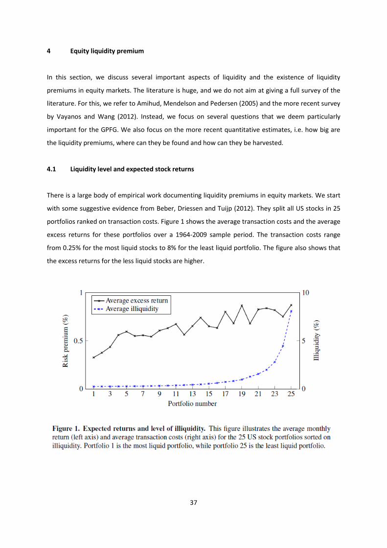
Traditionally, there has been fairly strong evidence that there are liquidity premiums in equity
markets; many studies document both liquidity level and liquidity risk premiums. In older studies,
these premiums tend to be large, with estimates around 6% per year. However, more recent studies
show that the liquidity level premium and other effects like size and value have substantially
diminished over the last decades. For NYSE stocks the liquidity premiums even seems to have
completely vanished; for NASDAQ stocks there is only a liquidity risk premium. The evidence for
other markets, like the UK, points in the same direction but more research on international markets
is needed. These liquidity premiums are mainly present in small cap stocks and in the least liquid half
of the market (which actually mostly coincide as illiquidity and size are strongly correlated). So, it is
not easy to profit from these premiums with large amounts of money.
In corporate bond markets there seem to be stronger effects of liquidity. A series of recent papers
document the existence of liquidity level premiums. Although their research methods differ, the
conclusions of all empirical works are quite similar. There are liquidity premiums in corporate bonds
with low credit ratings, and conditional on the credit rating in the least actively traded bonds. These
premiums are fairly large, up to 1% per year. In periods of market stress, such as the recent financial
crisis, the liquidity premiums are even higher. The transaction costs on corporate bonds are also
7
dramatically higher during the crisis. This highlights that the liquidity premium may come with large
temporary price fluctuations. However, the GPFG is in a unique position to weather these stress
periods, since there are no immediate spending needs and the investment horizon is longer than
that of the average market participant (who may be an insurance company subject to regulatory
constraints).
In the market for treasury and government agency bonds there are small liquidity premiums for off-
the-run bonds, which tend to be cheaper than the more liquid on-the-run bonds. The additional
returns from investing in off-the-run bonds are very small though (a few basis points), and it may be
better to buy treasury bonds at auction, where yields are typically somewhat higher than in the
immediately following secondary market trading. More striking in the fixed income market is the
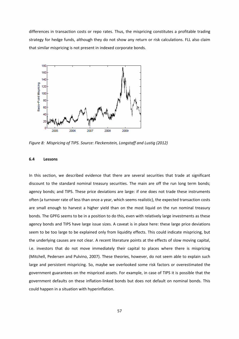
apparent mispricing of agency bonds and inflation indexed bonds (TIPS). Bonds of several
government guaranteed agencies in the US, Germany and France trade at large spreads above the
treasury bonds. Yield spreads range from 20 basis points in calm times to 70 basis points in the crisis.
These spreads are strongly correlated with measures of transaction costs, but seem to be too large
to be explained only from the higher costs of trading these bonds relative to treasury bonds. There
seem to be mispricing with as yet unknown explanation. These could form opportunities for the
GPFG because the issue sizes of these bonds are fairly large and the markets are fairly liquid.
We also investigate the presence of liquidity premiums in alternative investment classes. For hedge
funds, there is some evidence on the existence of a liquidity risk premium. This premium can be
quite substantial, several percentage points per year, but obviously investments in hedge funds carry
many other sources of risk, and profiting from a liquidity risk premium should not be the main
reason to invest in hedge funds. The evidence for listed real estate (REITs) is similar to the evidence
for equities with similar market capitalizations: there are modest liquidity and liquidity risk
premiums. No work is available yet for very recent data though, so it remains an open question how
large these premiums are nowadays. Other alternative assets such as direct real estate, private
equity and infrastructure investments are not listed and have no well-functioning secondary market.
This makes trading very costly and investors are forced to commit their investments for many years.
One would expect that only investors with long investment horizons are present in this market.
From a theoretical point of view, one would therefore not expect large liquidity premiums in the
market for private equity and other non-listed assets that are strongly correlated with liquid asset
markets. For private equity, there is no empirical evidence for a compensation for the expected
8
illiquidity of the investments, but there is some evidence for a liquidity risk premium similar to that
in hedge funds.
Finally, we discuss the results on time variation in liquidity and the relation to asset prices. There is
substantial time-variation in liquidity and transaction costs rise dramatically in times of financial
market stress. Asset prices fall in such periods, as liquidity and prices are contemporaneously
correlated. Recent papers have found that most of the liquidity premiums can be earned in down
markets; this seems to be the case in several asset classes such as equities, corporate bonds and
REITs. This evidence brings the about the question whether investors are able to profit from liquidity
and price fluctuations using dynamic trading strategies, in particular by buying additional illiquid
assets in stress times. Unfortunately, there is little systematic evidence yet that returns can be
predicted from past liquidity and for the profitability of such liquidity timing strategies. When
considering dynamic strategies with illiquid assets, the fund also has to consider that illiquid assets
may show large price drops in subsequent periods of market stress. Consistency in the asset
allocation policy is therefore required to profit from such a timing strategy.
Having seen this evidence, what do we recommend the Norwegian ministry of finance? Should the
mandate for the GPFG explicitly allow or impose investments in illiquid assets? Our
recommendations are the following:
1. There is limited scope for earning liquidity premiums in equity markets. Investing in illiquid
stocks seems appropriate as a part of a value weighted passive strategy, but the recent
evidence does not suggest that illiquid stocks generate significant outperformance. Notice
that there is also no reason to exclude illiquid stocks from the investment portfolio. There is
more evidence for the presence of a liquidity risk premium: stocks with large exposure to
market-wide liquidity fluctuations have higher expected returns than stocks with low
exposure. Estimates of the magnitude of the liquidity risk premium, however, differ quite a
bit across studies and sample periods.
2. In corporate bonds, there may be more scope for earning a liquidity premium, but here the
fund is hampered by its large size. Liquidity premiums are largest in speculative grade bonds
and in illiquid bonds. Both tend to have a decent issue size but high transaction costs. An
active trading strategy is therefore not recommended, but overweighting such speculative
grade and illiquid bonds in the overall corporate bond portfolio appears to be profitable.
9
3. In the class of treasury and government guaranteed bonds, agency bonds and TIPS seem to
deliver liquidity premiums, sometimes quite substantial. A caveat is that these premiums
seem to be too high to be only explained from liquidity and there may be unexplained risks.
4. There is not much strong evidence for the presence of liquidity premiums in alternative
asset classes. In hedge funds and perhaps private equity there seem to be liquidity risk
premiums. These premiums, however, have to be weighed against the sometimes very high
costs of investing in these asset classes and other sources of risk that these asset classes
entail. For non-listed securities there is no reliable evidence on liquidity premiums and we
cannot give a recommendation.
5. Liquidity considerations should also play a role for the rebalancing of positions, both at the
strategic and tactical level. Our literature study shows that positions in less liquid assets
should be rebalanced less often, and the rebalancing should typically be "partial" to limit the
costs of trading. Even low transaction cost levels can imply very low rebalancing frequencies,
and for large investors rebalancing trades should be relatively smaller when there is price
impact of trading large quantities. It is, however, difficult to make precise quantitative
recommendations when the investment portfolio has many correlated assets.
6. On the issue of dynamic strategies that exploit temporary price effects of liquidity, we find
that there is not enough evidence about the profitability and the risks of such strategies to
give a positive recommendation to implement these.
10
[This page is intentionally left blank]
11
2 Theory on liquidity and asset pricing
In this section we give an overview of the theoretical literature on asset pricing and liquidity. We
start in a setting where investors only trade twice, thus buying assets at a given date and selling
these assets one period or several periods later without trading at intermediate dates. In such a
setting it is possible to derive closed-form asset pricing expressions in a setting with multiple assets,
even when allowing for heterogeneity in the horizon of the investors. In this setting it is also
straightforward to incorporate liquidity risk. In these models illiquidity is modeled through the
transaction costs when buying or selling assets.
In the second part of this section we discuss models that allow for more complicated trading
strategies, such as rebalancing at intermediate dates or dynamic strategies to exploit time variation
in risk and return. Here most studies typically focus on a case with a single, representative investor
and a single risky asset.
Ideally, these theoretical models would both have dynamic and multi-period trading strategies,
multiple assets, and heterogeneous investors, but such models are hard to solve. The models
discussed in the first part of this section are thus mostly useful to understand the cross-sectional
pricing of liquidity. The models in the second part are informative on how liquidity affects dynamic
trading behavior.
2.1 Pricing liquidity effects without dynamic trading
2.1.1 Risk-neutral investors
We start in a setting without risk or, equivalently, with risk-neutral investors. Consider N assets
which have percentage transaction costs equal to ci, i=1,...,N. These are the costs of selling the
assets, which may incorporate direct trading costs and costs due to the bid-ask spread.
First consider the case where all investors have the same trading frequency or investment horizon.
Amihud and Mendelson (1986) consider an investor who may liquidate her portfolio in given period
with probability , so that the expected horizon is 1/ (see also the survey of Amihud, Mendelson,
12
and Pedersen (2005)). Beber, Driessen and Tuijp (2012) consider investors with a fixed horizon h.2 In
these cases, the gross expected return (gross of transaction costs) equals
( ) ( )
The return net of the (expected) trading costs then equals the risk free interest rate , which is the
risk-adjusted required rate of return for all assets since all agents are assumed to be risk neutral.
This model thus implies that expected gross returns increase linearly with transaction costs. The
term /h could be referred to as a liquidity premium, but it is important to note that this is purely a
compensation for costs and not an excess return. Of course, an atomistic investor who does not
affect market prices could generate an excess return if she has a longer horizon than the
representative investor, but for a large investor this is not a realistic assumption. Therefore we now
turn to a setting where investors have different trading frequencies or horizons.
Consider J different risk-neutral investors with decreasing trading frequencies μ1,…, μJ, and hence
increasing horizons h1=1/μ1,…, hJ=1/μJ. To derive the equilibrium returns, it is crucial whether the
investor with the longest horizon faces borrowing constraints or not. If this investor has no
borrowing constraints, then the equilibrium is simply that the investor with the longest horizon buys
all assets because she has the lowest expected transaction costs. Then the equilibrium expected
returns are
( )
Again the gross returns only reflect a compensation for trading costs and no excess return.
A more interesting equilibrium obtains when all investors have strict borrowing constraints. This is
the case studied by Amihud and Mendelson (1986). They show that in this case liquidity clienteles
are obtained: short-term investors exclusively hold liquid assets (with low transaction costs) while
only the long-term investors hold illiquid assets with high transaction costs. This model has two key
implications. First, it implies a concave relationship between expected gross asset returns and
2 Both Amihud and Mendelson (1986) and Beber, Driessen and Tuijp (2012) use an overlapping generations setting.
13
transaction costs. Second, the expected returns on illiquid assets, net of expected transaction costs,
exceed the net return on liquid assets (which are equal to the risk-free rate given the risk-neutrality
of investors). In other words, illiquid assets deliver a genuine liquidity premium for long-term
investors. The intuition for this result is that to persuade the long-term investors to buy the illiquid
assets, these assets must yield a return net of costs that is at least as large as the net return on liquid
assets.
These implications are best illustrated with a numerical example. Consider two assets with
transaction costs of 1% and 5%, respectively, and two investors with horizons of 1 year and 10 years.
The risk-free rate is 2%. In equilibrium, the more liquid asset is held by the short-term investors.
Since investors are risk-neutral, the return net of costs should equal the risk-free rate. The annual
gross expected return thus equals 2% plus 1% x 1 (the trading frequency), 3% in total.
The less liquid asset is held by the long-term investors in equilibrium. To make sure these investors
indeed prefer to hold illiquid assets, the return (net of costs) on this illiquid asset should be at least
the return on the liquid asset. For holding the liquid asset, the long-term investors would earn 3%
minus the trading costs (1% times the trading frequency, which equals 1/10), giving a return of 2.9%.
Hence, long-term investors would earn an excess return of 0.9%. The illiquid asset needs to generate
(at least) such an excess return. This implies that the gross expected return on the illiquid assets is
the sum of 2% (risk-free rate), 5% x 1/10 (trading costs) and 0.9% (liquidity premium), 3.4% in total.
This example shows that the illiquid assets provide a net excess return (liquidity premium) of 0.9%.
The size of this excess return depends on three variables. First, it depends negatively on the horizon
of the short-term investors. Second, it depends positively on the horizon of the long-term investors,
and third, it depends positively on the transaction costs of the liquid asset. Note that the transaction
costs on the illiquid asset itself do not directly influence this excess return.
2.1.2 Risk-averse investors and liquidity risk
In this subsection we turn to a setting with market risk and liquidity risk, combined with risk-averse
investors. Liquidity risk is modeled by allowing the transaction costs ci to change stochastically over
time. A substantial empirical literature has established that liquidity is time-varying and, importantly,
14
the liquidity of stocks tend to co-move suggesting that liquidity might be a market-wide risk factor
(see Chordia, Roll and Subrahmanyam, 2000).
The seminal asset pricing model with liquidity risk is by Acharya and Pedersen (2005).3 This model
can be viewed as extension of the CAPM with stochastic percentage transaction costs. As opposed to
the Amihud-Mendelson (1986) model, AP assume that all investors have a one-period horizon. Their
model implies the following expression for the expected return on asset i
( ) ( ) ( ) ( ) ( ) ( )}
Where is the market-wide return and the transaction costs on the market portfolio. The first
term, ( ), represents a pure compensation for expected transaction costs as in equation (1),
where in this case the horizon h is equal to one. The second term reflects the usual CAPM beta, i.e.
the covariance between the asset’s return and the market return. The final three terms represent
liquidity risk premiums. They provide compensation for covariance of the asset return with the
market-wide transaction costs, the covariance of the assets' transaction costs with the market
return and the covariance between asset costs and market-wide costs. Empirically, the return-cost
and cost-return covariances are typically negative, while the cost-cost covariance is usually positive,
so that all liquidity risk terms contribute positively to the expected return. The coefficient is
proportional to the investors’ risk aversion, which determines the equilibrium price of market and
liquidity risk.
Notice that this model has the strong assumption that investors sell all their assets at the end of the
investment period. A more realistic assumption is that investors have a horizon of multiple periods
h. The equilibrium pricing model then is (by approximation)4
( ) ( )
( ) ̃ ( ) ( ) ( ) ( )}
This is a generalization of the Amihud and Mendelson model in equation (1), augmented with
market and liquidity risk premiums. In this model, all investors hold the same optimal portfolio, the
3 An early paper about asset pricing with liquidity risk is Jacoby, Fowler and Gottesman (2000).
4 This model is a special case of the Beber, Driessen and Tuijp (2012) framework.
15
market portfolio. Similar to the discussion in section 2.1.1 an atomistic investor with a long horizon
could exploit the liquidity risk premiums by overweighting assets with high liquidity risk premiums.5
However, the presence of large long-term investor will change equilibrium expected returns.
Therefore we now turn to the model of Beber, Driessen and Tuijp (BDT, 2012) who extend the AP
model to a setting with investors that are heterogenous in their investment horizon.
In BDT there are mean-variance investors who differ in their investment horizon h, and who do not
rebalance their position at intermediate dates (as in Amihud-Mendelson (1986)). Transaction costs
are stochastic and i.i.d.6 They derive an equilibrium in which there is "partial segmentation". Long-
horizon investors invest in both illiquid assets and liquid assets (for diversification since they are risk
averse), while short-horizon investors only hold liquid assets because the transaction costs on the
illiquid assets are too high given their horizon. Hence optimal portfolios are not equal to the market
portfolio and depend on the horizon.
In contrast to Amihud-Mendelson (1986) there are no borrowing constraints in this model. Hence,
the model does not generate excess returns on illiquid assets for this reason. Instead, the model
generates various other liquidity (risk) premiums. To illustrate their results, we discuss here a
version of the model with two investors with horizon h1 and h2 respectively, and two assets, a liquid
asset with low transaction costs
and an illiquid asset with high transaction costs
. For the
liquid asset the equilibrium expected return is very similar to the AP liquidity CAPM, and
(approximately) equal to
[
]
[
]
(
)
Notice that the coefficient on expected costs is between 1/ h1 (with h1=1 in the AP model) and 1/ h2.
Because this asset is held by both investors, the expected liquidity premium reflects the holding
period of the "average investor". For the illiquid asset, first consider the case where the two assets
have zero correlation. In this case the expected return is (approximately) equal to
5 This argument assumes that transaction costs are mean-reverting, so that liquidity risk is relatively smaller for
long horizons. 6 The model assumes that trading can always take place at some level of transaction costs. However, the
model implies that assets with very high transaction costs (for example, private equity) are held by only long-term investors who buy and hold this asset for many periods without rebalancing. The model thus applies to unlisted assets as well, and does not require an arbitrage strategy that frequently trades the illiquid asset.
16
[
]
[
]
(
)
(
) (
)
The first term is the usual compensation for expected costs (and hence does not generate an excess
return net of costs). The second term is the standard compensation for market and liquidity risk (as
in AP). The third term is new and represents a segmentation risk premium. Because the illiquid asset
is only held by long-term investors there is imperfect risk sharing for this asset which increases the
expected return. The coefficient of the segmentation risk premium is strictly positive and higher
when there are less long-term investors or when these long-term investors are more risk averse.
This segmentation risk premium thus presents a direct excess return of long-term investors relative
to short-term investors.7
Then we turn to the case where the liquid and illiquid assets are correlated. Denote by
(
) (
)
the coefficients of regressing the illiquid asset returns on the returns of the liquid asset. Notice that
for many illiquid asset categories that one can consider in practice (such as illiquid stocks, corporate
bonds, and private equity) these exposures to the liquid stock market are fairly large. The
equilibrium expected return on the illiquid asset then equals
( ) [
]
[
]
[
]
7 It is insightful to see what happens when an investor with an “ultra-long horizon” enters a market with short-
horizon and long-horizon investors. Depending on the parameters, there are two possible scenarios: If the presence of ultra-long-horizon investors does not change the segmentation of assets, the segmentation premium is the same for the long-horizon and ultra-long-horizon investors, but the ultra-long-horizon investor will benefit more from this as she will optimally tilt her portfolio more towards illiquid assets. Alternatively, the market for illiquid assets may become segmented into two "sub-segments" where the ultra-long-horizon investor exclusively holds the most illiquid assets. In this case the segmentation premium is highest for these most illiquid assets.
17
(
)
(
) (
)
(
) (
)
This equation shows that two additional terms emerge. First, the expected liquidity effect for illiquid
assets is higher when there is positive correlation between liquid and illiquid assets. If liquid and
illiquid assets are highly correlated, their liquidity premiums are also connected. Second, the
segmentation premium is smaller when there is positive correlation between liquid and illiquid
assets, because the illiquid asset returns can be partially replicated by investing in liquid assets.
There are two interactions between the liquidity and segmentation premiums. First, if the
correlation between liquid and illiquid assets increases, the expected liquidity effect for the illiquid
assets increases and the segmentation effect decreases. Second, as investors are more risk averse
the liquidity risk premium and the segmentation premium both increase.
The BDT model has other implications that are not directly visible in the approximations described
above. Most importantly, in the BDT model the liquidity risk premiums become smaller as the
horizon of the long-term investors increases. The longer their horizon, the less they care about
liquidity risk and hence the smaller its risk premium in equilibrium.
2.1.3 Summary and key implications
In sum, expected returns are influenced by illiquidity in three ways.
1. The first component is the expected liquidity premium. In all models, this includes at least a
compensation for expected transaction costs. In the Amihud and Mendelson (1986) model,
the expected liquidity premium exceeds the compensation for transaction costs. This excess
liquidity premium is the result of heterogenous investors that are subject to borrowing
constraints. This excess liquidity premium thus depends on the tightness of borrowing
constraints, but also on the horizon of short-term investors (-) and long-term investors (+),
and the transaction costs on liquid assets (+). In the Beber, Driessen and Tuijp (2012) model,
18
there is a spillover effect: the expected liquidity of liquid assets affects the liquidity premium
of illiquid assets if liquid and illiquid assets are correlated.
2. The second component is a compensation for liquidity risk, which usually depends on three
liquidity covariances, see equation (3). As with all risk premiums, the size of these premiums
depends on the risk aversion of investors. Also, liquidity risk premiums are smaller when
(some) investors have longer horizons.
3. Third, illiquidity may lead to segmentation effects. If illiquid assets are only held by a subset
of the investors (investors with long horizons) then there is imperfect risk sharing for these
assets which increases expected returns. These segmentation effects are larger when the
illiquid assets have low correlation with liquid assets.
In addition to the above insights, these models can be used to provide guidance on in which markets
liquidity premiums can be expected. This is particularly useful when there are no good data
available, which is the case for several alternative investments (for example, infrastructure
investments). Two specific cases are useful here. First, consider very illiquid investments of which
the returns are uncorrelated with liquid asset returns (such as stocks and bonds). In this case,
equation (3) predicts a small expected liquidity premium but a large segmentation risk premium. A
long-term investor will then hold these illiquid assets and earn an excess return. Alternatively,
consider very illiquid investments of which the returns are strongly correlated with liquid asset
returns. If the transaction costs on these liquid assets are negligible, then the liquidity premium on
the illiquid assets is small (only a compensation for the trading costs of long-term investors) and the
segmentation risk premium will also be negligible. An asset category that may fit in this example is
private equity, because, as Phalippou (2011) discusses, private equity returns are quite strongly
correlated with the returns on liquid stocks. Empirically, there is indeed no evidence for a liquidity
level premium in private equity.8
2.2 Endogenous trade frequency
A maintained assumption in the theory of the previous section is that the trading frequency is
exogenous: although different across investors, their trading frequencies are not influenced by the
asset’s transaction costs and also not by the price of the asset. But one might suspect that investors
8 Franzoni, Novak and Phalippou (2011) do find evidence for a liquidity risk premium in private equity returns.
19
will endogenously trade less when transaction costs are high. In this section, we review a few key
contributions in this area.9
Constantinides (1986) considers a model like the consumption-saving model of Merton (1969) and
extends it with proportional transaction costs. In the Merton model, the investor optimally holds a
fixed portfolio weight in the risky asset. To maintain this fixed weight, the investor has to trade
continuously. With trading costs, this strategy is not feasible, as all wealth will be eaten up quickly by
the continuous trading. Instead, the investor reacts to these trading costs by rebalancing his
portfolio only infrequently. The results of Constantinides' model are quite neat:
The investor has a no-trading range. Only when the ratio of dollar wealth invested in the
risky asset and the value of the riskless asset holdings is outside this range does the investor
buy and sell the stock to get the ratio back within the range. The width of this range is
increasing in the transaction costs.
The average allocation to risky assets is decreasing in the transaction costs, as is optimal
consumption, but the effect on consumption is small.
The amount of wealth needed to compensate the investor for transaction costs is small.
Since the investor endogenously trades much less than in the Merton case, the
compensation needed for a 1% transaction cost is only an extra 0.2% annual return on the
risky asset for realistic parameters.
Liu (2004) performs comparative statics on the expected trading frequency. Not surprisingly, the
trading frequency is decreasing in the transaction costs. For realistic trading costs, the investor
trades very infrequently, around once a year. Liu does not calculate the turnover rate (the fraction
traded per year) of the stocks explicitly, but it will be much lower than the turnover rates we
observe in reality.10
An important limitation of Constantinides' and Liu's models is that there is no predictability or time
variation in investment opportunities. This is a serious limitation, as intertemporal hedge demands
would induce more frequent trading and probably a bigger role for transaction costs. Jang, Koo, Liu
and Loewenstein (2007) extend the analysis of Constantinides with intertemporal hedging demands.
They show that the presence of transaction costs can have first-order effects on the equilibrium
9 A more in-depth discussion of some of these papers can be found in de Jong and de Roon (2011).
10 Turnover rates in developed stock markets are around 100% nowadays.
20
price. The reason is that due to the hedging demands, the trading frequencies are not affected as
much by transaction costs. The expected trading costs over the investment period can now be much
larger than in the case without hedging demands. This would result in much larger illiquidity
discounts in the asset prices.
Garleanu and Pedersen (2012) present an asset allocation model with transaction costs that has
explicit analytical solutions. They model the transaction costs as in the Kyle (1985) model, i.e., as
price impact of trading, which is proportional to the trade size; hence total transaction costs are
quadratic in trade size. The optimal investment portfolio in their model consists of a weighted
average of (i) the mean-variance optimal portfolio and (ii) the portfolio in the previous period. The
weight on the optimal portfolio is bigger the more liquid the market is, and the adjustment is smaller
in illiquid markets. This result is quite nice because it is the only one (to the best of our knowledge)
that uses price impact as a measure for illiquidity. This seems to be a natural choice, as institutional
investors are fully aware of the impact that their large trades may have on prices. This structure also
neatly avoids the no-trade range results of the older literature.
2.2.1 Dynamic rebalancing
The models discussed above have specific implications for the optimal rebalancing strategies of
investors. Most of the literature focuses on the case of one risky asset. We can distinguish three
different assumptions on the transaction costs: (i) fixed costs per trade, (ii) transaction costs
proportional to the amount traded, and (iii) quadratic transaction costs (consistent with linear price
impact of trading). These cost structures generate different implications for the timing of
rebalancing and the amount traded when rebalancing takes place.
In terms of timing, both fixed and proportional transaction costs imply no-trading ranges (see Liu
(2004)). Only when the asset position falls outside this range, the investor trades. As discussed
above, the width of this range depends positively on the size of the costs. Liu shows that small cost
levels can already generate substantial no-trading ranges. For example, given standard assumptions
on risk preferences and asset returns, with $5 fixed costs and 1% proportional costs the no-trading
range equals $93500 to $152600. This implies a trading frequency of less than one year. The reason
for this result is that, from a risk-return perspective, holding a slightly suboptimal asset position is
not very costly.
21
The amount traded given fixed versus proportional costs differs however. With fixed costs only, the
investor rebalances to exactly the target portfolio weight. With proportional transaction costs the
investor only brings the asset position back to the boundaries of the range: if the asset position falls
below (above) the lower (upper) bound, the investor trades only the amount that brings the position
back to the lower (upper) bound.
With linear price impact (quadratic transaction costs) the implications are again different. As shown
by Garleanu and Pedersen (2012), the investor trades every period in this case, but only small
amounts: the investor rebalances towards the "target portfolio weight", but does not fully reach this
target portfolio. The amount of trading in each period depends on the distance between the current
position and target position and the level of the price impact, amongst others.
The literature on rebalancing with multiple assets is scarce (Liu (2004), Lynch and Tan (2010)), and
numerical results are only available when the number of assets is very limited. Liu (2004) shows that,
if the asset returns are independent from each other, the results for the single-asset case still hold
and trading rules are independent across securities. If asset returns are correlated, the trading rules
do interact. For example, if asset returns are positively correlated the no-trading range of a given
asset depends on the position in the other asset. If the position in this other asset is above the target
position, the no-trading range of the first asset shifts downwards.
With quadratic transaction costs Garleanu and Pedersen (2012) do obtain closed-form expressions
for the rebalancing rules with many assets, by making some specific assumptions on the asset return
processes, utility function and price impact structure. They show that the speed of adjustment
towards the target portfolio weights is decreasing in the price impact parameter and increasing in
risk aversion. The effect of risk aversion can be understood intuitively because larger risk aversion
makes deviating from the target portfolio more costly. Leland (2000) notices that the aversion to
deviations from the target can be larger than the risk aversion of the investor’s utility function. This
can be the case, for example, if the investor has tight restrictions on the tracking error relative to a
target portfolio, which is typically given by the strategic asset allocation. The effect of the wealth of
the investor is not immediately clear from the paper. In appendix A we present a stylized version of
the Garleanu and Pedersen (2012) model. From that analysis, it follows that a large investor will
22
adjust slower to the target portfolio than a small investor with the same relative risk aversion, simply
because the price impact of her trades is bigger.
In sum, this literature shows that positions in less liquid assets should be rebalanced less often, and
the rebalancing should typically be "partial" to limit the costs of trading. Even low transaction cost
levels can imply very low rebalancing frequencies. It is, however, difficult to make precise
quantitative recommendations when the investment portfolio has many correlated assets.
2.3 Lock-up periods and temporary illiquidity
In the case of lock-up periods, the illiquidity is caused by the inability to trade for a pre-specified
period of time. This happens, for example, after initial public offerings (IPOs), when the former
owners of the company are forbidden to trade their stake in an initial period after the IPO (often, six
months to one year). In the case of pensions and insurance, it is typically impossible or very difficult
to trade the pension or insurance contract before the retirement date (and often thereafter as well).
Also, investment vehicles such as private equity investments and hedge funds have lock-up and
notification periods, making it difficult to withdraw money from such investments.
The valuation of illiquid assets in such a setting has received much attention in the literature. There
are several theoretical contributions in this area, including Grossman and Laroque (1990), Longstaff
(2001) and Kahl, Liu and Longstaff (2003). These papers work from an equivalent utility approach,
which is sometimes also called an indifference approach. They compare an investor who has access
to a fully liquid asset to another investor, with the same preferences, who has a position in the
illiquid asset. The models specify the optimal consumption-investment strategies of the two
investors. The expected utility of the two investors is then compared. This approach can be used to
determine how much of the liquid asset the investor should be endowed with in order to obtain the
same expected utility as the investor with the illiquid asset. This value is then the value of the illiquid
asset.
The model of Kahl, Liu and Longstaff (2003) is a good and simple example of this approach. There are
three assets in the economy: a risk-free (cash) investment, a stock index fund and a stock in the
investor's firm. The investor can trade freely in the risk-free asset and the stock index fund, but his
holdings in the firm are restricted until time R. After R, the stock can be traded freely. Obviously, the
23
value of the restricted stock depends on the parameters of the model. Especially important are the
length of the lock-up period; the asset's volatility (the higher the volatility, the higher the illiquidity
discount); the correlation with the market (the higher the correlation, the lower the discount as the
market can be used as a hedge against the illiquid asset's return fluctuations); and the fraction of
initial wealth locked up in the illiquid asset (the higher this fraction, the higher the illiquidity
discount). For example, a two-year lock-up for an asset with 30% volatility and no correlation with
the market has a 10% discount for an investor with low risk aversion and half of his wealth locked up
in the firm's stock. For a five-year lock-up period, the discount rises to 28%. De Jong, Driessen and
Van Hemert (2007) use a similar approach to study the investments of a homeowner.
Longstaff (2001) models the impact of illiquidity on optimal investment by introducing a bound α on
the (absolute) fraction of shares that can be traded per unit of time. The strictest bound (α=0, so no
trading at all) corresponds to a buy-and-hold strategy. As wealth has to remain positive at all times,
the finite trading possibilities endogenously impose borrowing and short-sales constraints. This
restriction is not very costly if the Merton weight w (i.e. the optimal portfolio weight of the risky
asset in the absence of trading restrictions) is below one, but for cases with w>1 this restriction
leads to a significant decline in the certainty equivalent of expected utility. This can be translated to
a lower price that the investor is willing to pay for the asset (an illiquidity discount). For example,
when w=2, the discount is around 2.5%, and for w=5 the discount is around 15%. Obviously, such
high portfolio weights are unrealistic for a large and diversified investor such as the GPFG.
De Roon, Guo and Ter Horst (2009) show that lock-ups substantially reduce the utility of hedge fund
investments. Stocks and bonds can be traded every month, but the amount invested in hedge funds
is fixed at the beginning of the investment period and cannot be changed during the remainder of
the investment period. De Roon et al. then compare the expected utility of final wealth between this
setting and a setting in which there are no restrictions on trading hedge funds, i.e., the portfolio
weight in hedge funds can be adjusted every month. The paper finds that the lock-up period of three
months costs the investor around 4% in certainty equivalent return per year.11 Investing in multiple
funds with different starting dates (so called 'laddering') may mitigate the effects of illiquidity for the
11
This wealth effect seems very high. It is caused by the large allocation to hedge funds that the investor chooses in their model: without lockups, the portfolio weight on hedge funds would be 62%. Of course, this weight is much larger than most investors would choose, and with lower weights on the hedge funds the welfare losses will be a lot smaller.
24
portfolio as a whole, thereby reducing the utility loss. In an empirical study, Aragon (2007) shows
that hedge funds with lockups have a value that is 4-7% lower than hedge funds without lockups.
All these studies assume that the illiquid asset becomes liquid at some point and remains liquid ever
after. Ang, Papanikolaou and Westerfield (2011) notice that the effect of a liquidity crisis is different:
assets that were previously liquid suddenly become illiquid. They present a model with two assets.
One which is liquid and can always be traded and one which is illiquid and can be traded only at
random points in time, with average waiting period until the next trading period λ. The major
restriction in the model is that only the liquid asset can be used to pay for consumption and can be
used as collateral for leverage in the portfolio. The illiquidity of the second asset has two effects. The
first effect is that the investor will allocate less of his wealth to the illiquid asset (relative to the
model with two perfectly liquid assets). The second effect is that the investor will also allocate less
to the risky assets and invest more in the risk free asset; this is because the illiquidity of the second
asset makes the investor effectively more risk averse. This is the background risk effect of Grossman
and Laroque (1990). The paper does some calibration of the welfare losses of the possibility of a
financial crisis. The investor is willing to pay 2% of his wealth to avoid a crisis that happens once
every ten years, which lasts two years and in which an otherwise liquid asset becomes illiquid with
trade possibility only once a year (λ=1). This is actually a small welfare effect: it is equivalent to a 10
basis points higher expected return on all assets (assuming a duration of 20 years).
We now discuss some practical implications of these studies for the GPFG. It seems that the welfare
effects of lock-up periods and occasional liquidity crises are small, unless the investor is (i) heavily
invested in illiquid assets and (ii) these illiquid assets have little correlation with the liquid assets’
returns. But these aspects seem to be of modest relevance for the GPFG, which invests only a small
fraction of its wealth in (very) illiquid assets, and does not have a need to sell these assets in crisis
periods. Moreover, illiquid assets such as small cap stocks, corporate bonds, real estate and private
equity tend to have a high correlation with liquid stocks (see e.g. Driessen, Lin and Phalippou, 2012).
Therefore, the welfare losses (in terms of dynamically optimal asset and consumption allocation) for
the GPFG of modestly increasing the illiquid asset holdings appear to be very small.
25
3 Liquidity: measurement and time trends
In this section we discuss the background for the reasons of existence of illiquidity and the most
appropriate way to measure liquidity. We also give some descriptive measures of liquidity and its
variation over time.
3.1 Theoretical background
In order to address the question which liquidity matters, we need to discuss the possible sources of
illiquidity. Economic theory offers a number of explanations. The main theories can be classified in
three groups: order-processing costs, inventory and search costs, and asymmetric information.
Order-processing costs
Order-processing costs refer to the costs that financial intermediaries such as market makers,
dealers and exchanges make in processing orders. These could be costs like the back office,
exchange, broker and clearing fees and the like. With modern technology and increasing
competition between exchanges, these costs are likely to be low for heavily traded products such as
stocks, treasury bonds and large-issue corporate bonds. However, for structured products and in
smaller markets such as the municipal bond market and real estate markets, these costs may be
relatively high. For investors, order-processing costs also include any fees and taxes that are levied
by the exchanges or the government.
Inventory and search costs
Consider a typical financial market that is centered around a relatively small number of dealers.
Many financial markets have this structure, for example, the bond and foreign exchange market, the
options and futures markets and the market for block trades in equities. These dealers typically
trade on their own account and provide an important service to investors: the opportunity to trade
immediately without the investors having to search for a counterparty to their trade. The dealers are
thus liquidity providers. The cost of providing this immediacy is twofold. First, the dealers have to
invest time and effort to find a counterparty. Second, the dealers often are the counterparty to the
trade, until the lot is traded along to another investor, and in the meantime the dealer becomes the
owner of the securities. These have price risk, and dealers are most likely quite risk averse, as they
need to pledge their own capital as buffers against these risks. To compensate for the search cost
26
and the inventory risk, the dealers charge a fee to the investors. Although this can be an explicit fee
or commission, it is more usual for the dealer to charge different prices for buying the asset (a
relatively low bid price) and selling the asset (a relatively high ask price). The difference between the
bid and ask prices (called the bid-ask spread) is an implicit cost for the investors, as they buy at a
high price and sell at a low price. Conversely, the bid-ask spread is a profit for the dealers. In
competitive markets, the bid-ask spreads will be driven down to the level where the spread
compensates exactly for the search costs and the inventory risk of the dealers. In non-dealer
markets such as the modern electronic markets, the issuers of limit orders take the role of liquidity
providers. They face the same type of risks as the dealers, in the sense that their limit orders have
the risk of non-execution and do not immediately lead to a transaction, so there are waiting costs.
These lead to very similar effects as the inventory and search costs. The specific market mechanism
is therefore less important than the underlying economic mechanisms to explain transaction costs.
Asymmetric information
In many markets, the initiators of transactions know more about the quality of the goods than the
potential counterparties do. A classic example is Akerlof's (1970) market for 'lemons', where the
sellers of used cars are much more aware of the quality of the car than potential buyers are. To
protect themselves from buying a 'lemon' (i.e. a low quality car), the buyers bid lower prices than in
a situation with symmetric information. In financial markets, the situation is not very different. Some
traders may be better informed than others. However, these informed traders may be on both sides
of the market (i.e. they may be buyers or sellers). The presence of such informed traders leads to a
wedge between buying and selling prices. In the famous model of Kyle (1985), the prices are linear in
the size of the order
( ) λx
where x is the size of the order (x>0 indicates a buy, and x<0 a sell). The coefficient λ is the price
impact of a trade, and indicates how much the transaction price is affected by the order. A high
'lambda' indicates a large price impact and an illiquid market in which small orders can move prices
substantially. Interestingly, this price impact is permanent and not reversed in later trades. Kyle's
lambda is an often-used measure of transaction costs in the empirical literature.
27
For the question of earning liquidity premiums on equities, the source of illiquidity does not matter,
only the effect on the expected returns is important. However, for the trading strategies the source
of illiquidity may be important: adverse selection and inventory costs lead to price impact and
quadratic transaction costs. According to Garleanu and Pedersen (2012), the best trading strategy
then is slow but continuous adjustment to the optimal portfolio. On the other hand, if illiquidity is
mainly caused by rents of the intermediaries, the transaction costs will be proportional in nature and
the literature suggests (sometimes wide) no trade ranges and infrequent rebalancing. Given the size
of the GPFG, the price impact of trades in illiquid markets appears to be the main concern.
3.2 Measures of liquidity
Based on the theoretical background, there are basically three types of liquidity measures:12
1. Measures of price reversal (‘gamma’ measures in the language of Vayanos and Wang, 2012).
These measure the round-trip cost of buying and then immediately selling a stock.
2. Measures of price impact of a transaction (‘lambda’ measures in Vayanos and Wang’s terms,
named after the price impact measure developed by Kyle (1985)). These measure how much
a trade moves the price of an asset; this measure of liquidity is particularly important for
institutional investors since they usually trade large orders which may move the price of an
asset.
3. Measures related to the trading activity. Such measures do not directly measure trading
costs, but may be a proxy for the effort it takes to find a counterparty for a transaction
(search costs).
Examples of ‘gamma’ measures
Bid-ask spread: quoted spread, effective spread and realized spread. Estimating these
requires high-frequency transaction data, which are not always available for all markets or
for a long time span (although increasingly so). Calculating these measures is also quite time-
consuming. Therefore many other measures based on daily data have been developed
Roll’s (1984) measure of price reversal, based on the covariance between subsequent (daily)
returns. The idea is that with high bid-ask spreads, transaction prices bounce up and down
between bid and ask price, which leads to a negative serial correlation in measured (trade-
12
We omit the technical details of the calculation of these measures. We refer to Chapter 6 of de Jong and Rindi (2009) for a detailed exposition about liquidity measures and how to estimate these.
28
to-trade) returns. Roll bases his measure on the square root of the negative of the estimated
covariance of daily returns with the previous day return. Hasbrouck (2009) refines this
measure and develops a Bayesian estimation method to ensure that it can also be calculated
if the covariance is positive.
Pastor and Stambaugh (2003) define a measure of price reversal after large transactions.
This is based on a similar idea, but works out slightly differently as the coefficient in a
regression of the return on an asset on volume of trading in the asset the previous day,
signed with the direction of previous day’s return (positive or negative).
Examples of ‘lambda’ measures
The most accurate measure of price impact is the permanent-variable component of the bid-
ask spread, estimated from the Glosten and Harris (1998) model (described in Appendix B).
This measure has been popularized by Sadka (2006). He makes available on his website a
monthly measure of market-wide price impact, which can be used as a liquidity factor in
performance analysis. Like the effective and realized spread measure for gamma, Sadka’s
measure for lambda requires intraday data.
A measure based on daily data is the ILLIQ measure proposed by Amihud (2002), sometimes
simply referred to as the Amihud measure. ILLIQ is the average over some period (typically,
one or three months) of the daily absolute price changes divided by daily trading volume.
Thus, ILLIQ measures how much prices move as the result of trading volume. This measure is
easily calculated and very popular in recent empirical studies in finance.13
Examples of trading activity measures:
Trading volume or turnover (trading volume divided by market capitalization);
Lesmond, Ogden and Trzcinka (1999) propose to use the fraction of days with zero trading
volume in a given period as measure of liquidity;14
The PIN measure of Easley and O’Hara also falls in this category. This measure is based on
the daily imbalance of buy and sell orders, which in their model proxies for the presence of
an informed trader in the market (hence the name, Probability of INformed trading)
13
Sometimes, this measure is scaled by an index of total market capitalization to take out the strong downward time trend in trading volume (see for example Acharya and Pedersen, 2005). 14
Lesmond et al. interpret this measure as the implicit cost of not moving the price of the asset.
29
The question of course is which of these empirical measures are good (if any) and which one is the
best? Vayanos and Wang (2012) present a very general model of market liquidity. In that model
illiquidity can arrive from a variety of sources, such as participation costs, explicit transaction costs,
asymmetric information, imperfect competition, funding constraints and search costs. Vayanos and
Wang show that most of these underlying sources affect the price impact of trading (lambda), but
only some sources affect the price reversal (gamma). Price impact therefore seems to be the most
appropriate liquidity measure. Interestingly, in his study of liquidity risk Sadka (2006) finds that the
permanent-variable component of the bid-ask spread (the lambda) is the priced liquidity factor, and
the transitory component of the bid-ask spread (the gamma) is not priced.
Hasbrouck (2009) and Goyenko, Holden and Trzcinka (2009) run a battery of comparisons of
different liquidity measures. These studies assume that the effective spread and price impact
measures based on intraday data are the most accurate liquidity measures. These are used as
benchmarks and the liquidity measures based on daily data are seen as proxies. Both papers report
cross-sectional correlations between the benchmarks and various proxies. Hasbrouck (2009) reports
that the Amihud measure correlates strongly with the effective spread and so does his own version
of the Roll measure (see Table 1).
Rank correlation
cTAQ cGibbs Proportion of zero returns
Pastor-Stambaugh
Amihud’s ILLIQ
cTAQ 1 0.872 0.770 0.735 0.937
cGibbs 1 0.620 0.577 0.778
PropZero 1 0.363 0.598
PS 1 0.704
ILLIQ 1
Table 1: Spearman rank correlations between various measures of illiquidity. cTAQ is the effective spread estimated from intraday data on trades and quotes; cGibbs is the transaction costs estimate from daily return data using Roll’s model and Hasbrouck’s (2009) Bayesian Gibbs sampling method. Source: Table III in Hasbrouck (2009). Goyenko et al. prefer a number of less-known liquidity measures; they claim that the ‘effective tick’
of Holden (2009) and the ‘proportion of zero returns’ of Lesmond, Ogden and Trzcinka (1999) are
good measures of liquidity. So far, these measures have not been used much in empirical work,
although the proportion of zero returns is popular in research about international markets, which
we discuss in section 4.4. The effective tick measure seems obsolete, now that most exchanges
implemented decimalization or otherwise substantially reduced the minimum price variation. Out of
30
the more conventional measures, Goyenko et al. find Roll’s estimator and Hasbrouck’s version of it
to correlate quite strongly with the effective spread; the Amihud measure correlates the best with
the price impact measure. The ‘proportion of zero returns’ measure is also positively correlated with
the benchmarks, but the Pastor-Stambaugh measure is not significantly correlated with the
benchmark liquidity measures. These findings are based on cross-sectional correlations, but in the
time series dimension the findings are pretty similar, see Table 2. Note that these studies all use
data from the US equity market.
Time-series correlation
cTAQ cGibbs Proportion of zero returns
Pastor-Stambaugh
Amihud’s ILLIQ
cTAQ 1 0.635 0.750 -0.182 0.664
Table 2: Time-series correlations between various measures of illiquidity. Source: Table 2 in Goyenko, Holden and Trzcinka (2009).
Dick-Nielsen, Feldhutter and Lando (2012) perform a comparison of various liquidity measures for
corporate bonds. They find that the Amihud measure and their own implicit round trip cost (ICT)
measure do fairly well, but the Roll measure and trading volume are not so good. The main criterion
for this judgement is the behavior of the measures in the 2008-2009 financial crisis: the Amihud and
IRC measures spike up, whereas Roll and trade volume do not change much during the crisis.
There are not many studies comparing the performance of various liquidity measures in terms of
asset pricing. Duarte and Young (2009) estimate a model of stock pricing with liquidity as a
characteristic, using PIN and Amihud as liquidity measures. He finds that Amihud explains the cross-
section of expected returns better than PIN. In studies of liquidity risk, the most popular measures
are the Pastor-Stambaugh and Sadka measures, for which traded factor portfolios are available on
WRDS. Some papers, including Acharya and Pedersen (2005) and Bongaerts, de Jong and Driessen
(2011) use an equally weighted average of the Amihud price impact measure. Whether different
measures produce different outcomes is not clear. Goyenko et al (2009) report fairly high time series
correlations between the equally weighted averages of various liquidity measures (effective spread,
Roll, and Amihud). Again, the Pastor and Stambaugh measure is an exception and it is only weakly
correlated with the other measures. Sadka (2010) in his study of hedge funds uses several of these
measures and concludes (from his Table 8) that they give pretty similar results (the strongest results
are produced by the Sadka (2006) permanent-variable price impact measure).
31
Korajczyk and Sadka (2008) compare the ability of various liquidity measures to find liquidity
premiums, including both liquidity risk and liquidity as a characteristic in the model. Their measures
of liquidity include the Amihud measure, turnover, quoted and effective spread and the four spread
components of the Glosten-Harris model (permanent/transitory and fixed/variable). As for the
pricing of liquidity risk, they find that the first principal component of these series is the best
measure of market liquidity. This measure consistently produces a liquidity risk premium in the cross
section of stock portfolios sorted on exposure to this factor. The measure-specific liquidity
component does not carry a risk premium for any of the measures. Liquidity as a characteristic is
only priced for the Amihud and turnover measures, not for the others.
All in all, we can conclude from these studies that the measures of illiquidity based on daily data, in
particular Amihud’s ILLIQ measure and Hasbrouck’s version of Roll’s measure, are suitable for the
purposes of estimating liquidity premiums and liquidity risk exposures.
Finally, we note the following. The standard implementation of the Amihud (2002) measure is to
divide daily absolute returns by daily volume (measured in dollars or other currency units). Goyenko,
Holden and Trzcinka (2009) suggest applying the division by volume also to other liquidity measures,
such as the effective spread or Roll’s estimator. This procedure is used by Ben-Rephael et al. (2012)
who use two versions of Roll’s estimator in their study: the ‘raw’ measure and the one divided by
trading volume. However, the division by dollar volume makes the Amihud illiquidity measure (or
any other measure scaled by dollar volume) by construction lower for large firms and higher for
small firms. Brennan, Huh and Subrahmanyam (2012) have argued that this feature makes such
liquidity measures accidentally pick up size effects. Instead, they suggest calculating Amihud’s
measure as the ratio of absolute return to turnover, where turnover equals trading volume divided
by the market capitalization of the stock.15 Florackis, Gregoriou and Kostakis (2011) argue that also
from a theoretical point of view this alternative definition seems justified, because in the standard
liquidity asset pricing model, see equation (1), the parameter µ is the asset’s turnover (trading
frequency) and the illiquidity variable ci thus should measure the transaction costs per unit of
turnover.
15
Notice that this is different from scaling the Amihud measure by total market trading volume.
32
3.3 Time variation in liquidity
It may be illuminating to see what level of transaction cost one observes in practice. Ben-Rephael,
Kadan and Wohl (2012) provide recent estimates for US equities, based on data from 2010. The
estimated cost of a transaction is around 20 basis points for NYSE stocks and around 40 basis points
for NASDAQ stocks. These numbers are equally weighted averages across all stocks and therefore
reflect the costs of trading an ‘average’ stock in these markets. Degryse, de Jong and Van Kervel
(2013) report effective half-spreads of 12.5 basis points for a sample of Euronext Amsterdam stocks
over the period 2006-2009. These stocks have an average market capitalization about twice that of
the average stock at the NYSE.
For the GPFG, these cost estimates may be viewed as a lower bound because the fund typically
trades large quantities. Large trades also have some price impact, which can erode profits from
strategies that are aimed at buying undervalued (or selling overvalued) assets, since the very trading
can move the prices up (down) and spoil the opportunity. Bikker, Spierdijk and Van der Sluis (2007)
have estimated the implementation shortfall of trades of a very large Dutch pension fund, using
proprietary data from 2002. They find transaction costs of 20 basis points for buys and 30 basis
points for sales. These numbers are similar to the estimates for the most liquid securities in the
market, which is not surprising as this pension fund trades mostly in large cap, liquid securities.
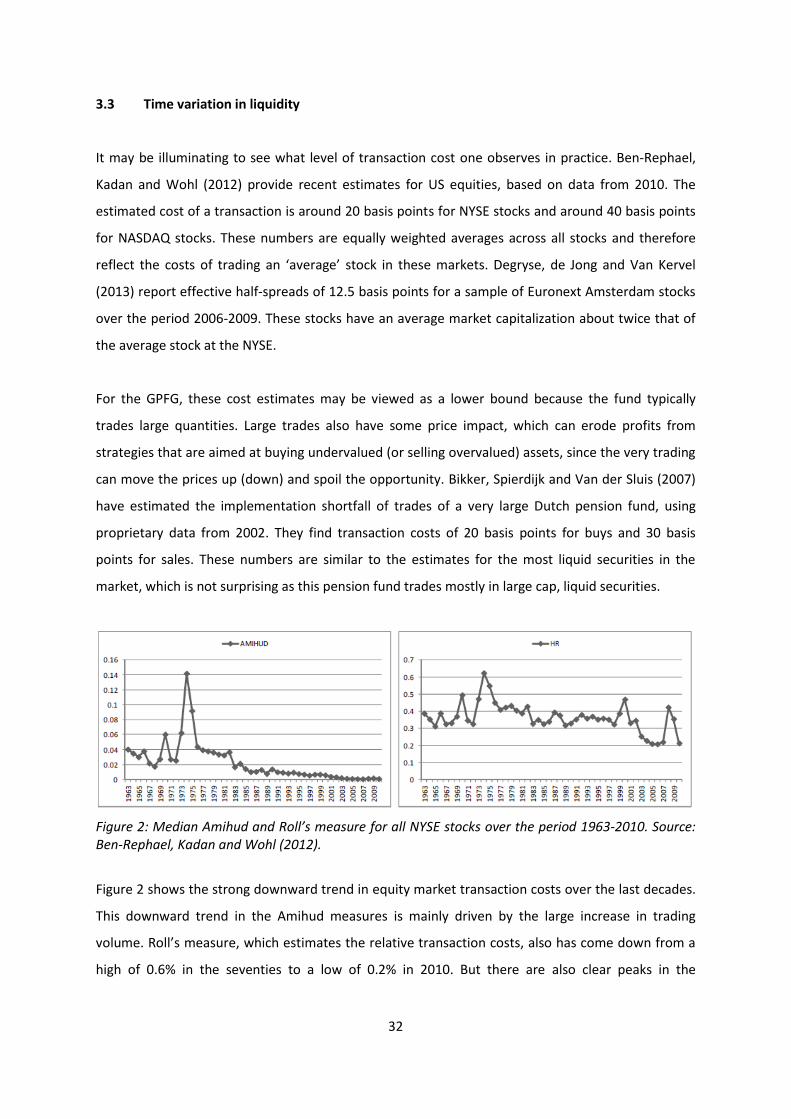
Figure 2: Median Amihud and Roll’s measure for all NYSE stocks over the period 1963-2010. Source: Ben-Rephael, Kadan and Wohl (2012).
Figure 2 shows the strong downward trend in equity market transaction costs over the last decades.
This downward trend in the Amihud measures is mainly driven by the large increase in trading
volume. Roll’s measure, which estimates the relative transaction costs, also has come down from a
high of 0.6% in the seventies to a low of 0.2% in 2010. But there are also clear peaks in the
33
transaction costs, coinciding with periods of market stress around the 1998 LTCM crisis and the
2008-2009 financial crisis.
Like the liquidity in stock markets, corporate bond liquidity fluctuates strongly over time. Figure 3
illustrates this: before 2007, average trading costs on corporate bonds were around 0.5%. In the
crisis, the costs shot up to 3%.
Figure 3 Transaction cost on corporate bonds. Source: Bongaerts, de Jong and Driessen (2011)
Chordia, Roll and Subrahmanyam (2000), Hasbrouck and Seppi (2001) and Huberman and Halka
(2001) show that the fluctuations in liquidity have a strong common component, i.e. the fluctuations
in liquidity tend to be positively correlated across stocks. Lee, Karolyi and Van Dijk (2012) provide
more evidence for commonality in liquidity for a large number of developed and emerging stock
markets. If shocks to liquidity are common, liquidity could be a priced risk factor. We shall discuss
evidence on that later in section 4. In this subsection, we discuss the patterns and possible causes of
time variation in liquidity in more detail.
The main driver of time variation in liquidity is the volatility of the asset returns. This can be
explained from several theories. Traditional models of inventory management by risk-averse dealers
(see for example Ho and Stoll, 1981) predict a strong relation between transaction costs and
volatility. The bid ask spread is compensation for dealers inventory risk, and is proportional to
0.00%
0.50%
1.00%
1.50%
2.00%
2.50%
3.00%
3.50%
Pe
rce
nta
ge
tran
sact
ion
co
sts
Corporate bond market liquidity: Roll/Hasbrouck measure
34
variance. More recent work looks at the relation between funding liquidity (i.e., the availability of
capital) and market liquidity. Trading in markets requires capital, and the cost of capital is higher
when volatility is higher. Brunnermeier and Pedersen (2009) model this through a value at risk
constraint, which becomes tighter when volatility increases. This restriction increases the cost of
trading and hence reduces liquidity. This can actually reinforce the funding constraints, leading to
downward liquidity and price spirals. Aragon and Strahan (2012) show an interesting example of the
relation between market liquidity and funding liquidity. After the Lehman bankruptcy, hedge funds
that used Lehman as their prime broker faced an unexpected funding liquidity shock. That caused
fire sales, which reduced the market liquidity of the assets sold.
Nagel (2012) studies the returns on a simple short-term price reversal strategy: buy stocks that
decreased in price yesterday, and sell stocks that increased in price. If the portfolio weights in such a
strategy are proportional to yesterday’s return, the profits from this strategy are equal to minus the
cross-sectional average first order serial covariance in daily stock returns. Notice that this is exactly
the ‘gamma’ liquidity measure as defined by Vayanos and Wang (2012) and is the basis of Roll’s
estimator, which is just the square root of this gamma measure. In that sense, the reversal can be
interpreted as a measure of average transaction costs in the market and as the reward to providing
liquidity. Nagel shows that there is a very strong correlation between the price reversal measure and
the VIX index. This is of course perfectly in line with inventory theories where risk-averse market
makers require a compensation for liquidity provision proportional to the volatility of the assets.
Although Nagel does not provide evidence on liquidity premiums, one can expect the liquidity
premium to be larger in times where the cost of providing liquidity is higher.
Naes, Skjeltorp and Odegaard (2011) relate the time variation in liquidity to business cycle
fluctuations. They show that investors’ portfolio composition changes when liquidity falls and their
adjustments point at a flight to quality effect. These findings give some insight into the causes of
commonality in liquidity.
Following this evidence on time variation in liquidity, Ang (2013) suggests that dynamic investment
strategies can pick up liquidity premiums. This argument relies on liquidity effects in prices being
temporary and reverting within a reasonable amount of time. The events in the 2008/9 crisis give
some indication for the presence of temporary liquidity effects. Lou and Sadka (2011) document that
realized equity returns in the crisis depend strongly on the liquidity risk exposure. This is not
35
surprising, as the liquidity factor itself showed large movements in the crisis. It is however not
obvious that such temporary liquidity effects are also present in other periods. Moreover, there is
not much systematic evidence on whether liquidity fluctuations lead to predictable effects in asset
prices. Amihud (2002) shows that stock returns are positively related to the liquidity of that stock in
the previous year or month. But as current liquidity is strongly related to past liquidity, this may
simply pick up the liquidity level premium (this is in fact Amihud’s interpretation of this result).
Bekaert, Harvey and Lundblad (2007) offer some evidence for the predictability of stock market
returns using lagged market liquidity. Using a VAR model with monthly data for a sample of
emerging markets, they show that next month’s value weighted market return is negatively related
current market liquidity. For the U.S. market, however, this effect is not significant. Also, there may
be other reasons why there are temporary price effects and predictability, such as the well-known
momentum effects and book-to-market effects or long horizon price reversals. The former works
over a horizon of 6-12 months, the latter over a horizon of 3-5 years. Any systematic liquidity timing
strategy should take such effects into account and we are not aware of good research about this.
Therefore, even though this is an interesting and potentially promising strategy for long-term
investors, we find it too early to give recommendations about this idea.
3.4 The influence of changes in market structure
One very clear pattern over the last decades is the strong decrease in trading costs. As discussed
before, many developments in markets have contributed to this, such as moving to electronic
trading, decimalization, increased transparency and competition between exchanges. In the last
years, the most important developments in markets are the rise of High Frequency Trading and the
fragmentation of trading over multiple trading venues. Several studies have looked at the impact of
these developments on market quality.
Hasbrouck and Saar (2012) study the impact of high frequency trading on traditional measures of
market quality such as bid-ask spreads, depth and short term volatility. They study both normal
times and times of increased economic uncertainty, when there may be more stress in the market.
The latter is important, because high-frequency traders often act as (voluntary) market makers, who
are likely to improve the market in calm times but may leave the market in stressful times.
Nevertheless, Hasbrouck and Saar find that low-latency trading is associated with improved market
quality, both in calm and in stressful times.
36
Degryse, de Jong and van Kervel (2013) investigate the impact of increased competition between
financial markets. They look at the European markets, where competition substantially increased
after the Markets in Financial Instruments Directive (MiFID) came into effect in November 2007.
Degryse et al. use a variety of spread and depth measures as indicators of market quality. They find
that increased competition between open limit-order book (OLOB) based trading platforms, i.e. the
traditional exchanges and Multilateral Trading Facilities (MTF) like Chi-X and BATS, improves overall
liquidity. A caveat here is that to profit from this improved overall liquidity, traders need to have
access to all trading platforms, which requires costly technology such as smart order routers (SORT).
Thus, the improvements in liquidity are most relevant for professional and institutional traders. For
retail traders, who typically only access the traditional exchange, the picture is less clear and
liquidity for that group may even have decreased.
A final development we discuss here is the increase in dark trading. This is trading on for example
dark pools but also trades internalized by banks or brokers and OTC trading. In contrast to the visible
trading on exchanges and MTF’s, such dark trading has very limited transparency and its impact on
market quality is under debate. O’Hara and Ye (2011) and Buti, Rindi and Werner (2011) find that
dark trading does not harm liquidity, or even improves it, whereas Degryse, de Jong and van Kervel
(2013) find negative effects of dark trading on liquidity.
Despite all these changes in markets, the traditional measures of transaction costs like effective
spreads, depth etc. still seem to be very useful for judging market quality. Quoted spreads and depth
at the best quotes are less useful though, because the high frequency traders place many orders
that tend to be very small; the best price may therefore be available only for very small quantities.
So, for institutional investors who place large orders, measures like effective spreads (which are
based on actual transactions), depth beyond the best quotes, and price impact are the most relevant
measures. One has to be careful though aggregating the available liquidity over several markets,
because high frequency traders can easily withdraw or adjust limit orders and a trade on one market
may lead to a reduction of liquidity on other markets (see Van Kervel, 2012, for a discussion).
37
4 Equity liquidity premium
In this section, we discuss several important aspects of liquidity and the existence of liquidity
premiums in equity markets. The literature is huge, and we do not aim at giving a full survey of the
literature. For this, we refer to Amihud, Mendelson and Pedersen (2005) and the more recent survey
by Vayanos and Wang (2012). Instead, we focus on several questions that we deem particularly
important for the GPFG. We also focus on the more recent quantitative estimates, i.e. how big are
the liquidity premiums, where can they be found and how can they be harvested.
4.1 Liquidity level and expected stock returns
There is a large body of empirical work documenting liquidity premiums in equity markets. We start
with some suggestive evidence from Beber, Driessen and Tuijp (2012). They split all US stocks in 25
portfolios ranked on transaction costs. Figure 1 shows the average transaction costs and the average
excess returns for these portfolios over a 1964-2009 sample period. The transaction costs range
from 0.25% for the most liquid stocks to 8% for the least liquid portfolio. The figure also shows that
the excess returns for the less liquid stocks are higher.
38
Based on such data, several papers provide formal estimates of the liquidity premium. Amihud and
Mendelson (1986) find that a 1% increase in the bid-ask spread increases expected returns by 2.4%
per year. Brennan and Subrahmanyam (1996) find that the lowest liquidity quintile stocks have an
average return (corrected for other risk exposures) that is 6.6% per year higher than the highest
liquidity quintile stocks. Amihud (2002) and Acharya and Pedersen (2005) also document significant
liquidity premiums in US equities. The latter paper finds a premium of 4.5% per year on the most
illiquid assets compared to the most liquid assets.16 Brennan, Huh and Subrahmanyam (2012) split
the Amihud measure in two half measures, for days with positive and negative returns. They find
that only the down-day Amihud measure is priced in the cross-section. They do not look at sample
splits for more recent years, though. Brennan, Huh and Subrahmanyam (2013) find very similar
results when they split the PIN measure between up and down return days.
More recent evidence for liquidity premiums comes from Ibbotson, Chen, Kim and Wu (2012). They
use turnover as a measure of liquidity. They construct a portfolio that consists of long positions in
stock from the lowest turnover quartile, and short positions in stocks with the highest turnover. This
long-short portfolio has an excess return of 5.34% per annum, and an outperformance relative to
the Carhart four-factor benchmark of 31 basis points per month, which translates to 3.73% per
annum. Ibbotson et al. also show that these differences in performance between high and low
liquidity stocks are there when one conditions on the size, value or momentum of the stocks. Using
double sorts on these variables and liquidity, they show that in almost each size etc. quartile, the
low liquidity stocks outperform the high liquidity stocks. An interesting result in that paper is that
these high-low liquidity strategies do not lead to a very high turnover. With annual rebalancing, 75%
percent of the stocks remain in the same liquidity quartile. This is similar to the turnover rate of size
and value strategies. The costs of implementing a high-low liquidity strategy are therefore likely to
be modest, although Ibbotson et al. do not present any calculations of the implementation costs.
16
A note on the research methodology: Typical studies in this area create portfolios of equities sorted according to some measure of liquidity, and then compare the average historical returns for the portfolios with the most liquid assets and the least liquid assets. Of course, these portfolios could be different in other respects than only liquidity and corrections for such differences have to be made. For example, illiquid assets tend to have smaller market capitalization that highly liquid assets and it is well known that small forms outperform large firms (the so-called size effect). Hence, to get a clean measure of the liquidity premium, one needs to control for differences in the other aspects of the portfolio. This can basically done in two ways: by applying double sorts to create portfolios (for example, first sort on size and the split every size portfolio according to liquidity) or by controlling explicitly for the different size etc. characteristics in the measurement of outperformance. This is typically done either by including size as a characteristic in the regressions or by including the Fama-French SMB factor in the benchmark model. Corrections for other characteristics (value, momentum, idiosyncratic volatility etc.) can be done in a similar way.
39
A natural question that arises at this point is the feasibility for a large investment fund like the GPFG
of strategies buying the least liquid stocks. In the study of Beber, Driessen and Tuijp (2012), the two
lowest liquidity portfolios (out of 25) of stocks listed on NYSE-AMEX, account for only 0.5% of total
market capitalization, with an average firm size of 250 million dollars and one-way transaction costs
above four percent.17 According to World bank data, the market capitalization of all US equities at
the end of 2011 was 15,000 billion dollars, so these least liquid portfolios have a market cap of at
most 75 billion dollars.18 This of course makes it difficult to put significant amounts of money in a
strategy to buy illiquid stocks.
Although many papers have documented the existence of a liquidity premium in US stocks, this view
is challenged by Ben-Rephael, Kadan and Wohl (2012). They study the evolution of liquidity
premiums in US equities over time. First, they establish (as many papers have shown) that liquidity
has improved dramatically in the last decades, and especially since the 1990’s when many exchanges
implemented reforms that reduced transaction costs substantially (see section 3.4). But the real
question is whether the liquidity premium (i.e. the expected return difference between high liquidity
stocks and low liquidity stocks) has changed. Ben-Rephael et al. show that this is indeed the case.
For stocks listed on the NYSE, the liquidity premium for an average liquid stock was 16 basis points
per month in the period 1964-1974, but in the period 1997-2008 this liquidity premium has
completely disappeared. For NASDAQ stocks, the liquidity premium was 11 basis points per month in
1986-1996, in the following decade it declined to 6 basis points. Another way to show the result is by
the ‘alpha’ of a long-short strategy where stocks in the least liquid decile are bought and in the most
liquid decile are sold. This strategy on NYSE stocks had an alpha of 61 basis points per month in
1964-1974, and an alpha very close to zero in 1997-2008. The similar strategy on NASDAQ had an
alpha of 98 basis points per month in 1986-1996 and 21 basis points per month in 1997-2008.
Hence, the reward to holding illiquid US stocks has decreased substantially over time. The addition
of recent data (up to 2011) does not change their results on the liquidity level effects: in recent
years, there seems to be no liquidity premium. They do find liquidity effects in penny stocks (stocks
priced below 2 dollars), but these stocks make up for only 0.2% of market capitalization.
17
We thank Patrick Tuijp for this calculation. The sample excludes stocks with prices below 5 dollars, so many very small cap stocks are not included in this breakdown. Notice also that the equities listed on NYSE-AMEX are typically larger than those listed on NASDAQ, and probably also bigger than firms listed in non-US markets, so these numbers on market cap refer to the least liquid segment of the most liquid market. 18 The total market cap data are found on http://data.worldbank.org/indicator/CM.MKT.LCAP.CD.
40
Ben-Rephael, Kadan and Wohl (2012) offer two explanations for the decline of the liquidity level
premium: (1) the increased use of ETF’s and (2) the increase in arbitrage activity with strategies
exploiting liquidity premiums. Further support for the latter explanation is given by Chordia,
Subrahmanyam and Tong (2012), who document that many of the well knows anomalies in equity
markets (size, value and momentum) have decreased in magnitude over the last years. If there are
any of such effects in the more recent years, they tend to be concentrated in the less liquid stocks,
i.e., the half of the sample with ILLIQ above the median. Although the paper does not directly focus
on liquidity premiums, they also find that effects of liquidity (ILLIQ) are concentrated in the less
liquid half of the stocks. Interestingly, the coefficient of ILLIQ in the cross-sectional regressions does
not seem to change much over time (the liquidity premium might well have decreased since ILLIQ
has fallen substantially, but they do not report any numbers). In the most liquid half of the stocks
there appears to be no liquidity premium. For the GPFG, these results are very relevant because the
stocks with illiquidity below the median are typically small and make up for only 10% of total market
capitalization.
4.2 Liquidity risk premiums
The studies discussed so far look at the effect of the level of a stock’s liquidity on its expected return.
Apart from the liquidity level effect, liquidity can also be a risk factor. The most common way to
measure liquidity risk is by the covariance of an asset’s return with a measure of surprise changes in
market-wide liquidity. This is indeed one of the three liquidity risk factors identified by Acharya and
Pedersen (2005) and also the factor that follows from multi-factor asset pricing models such as the
one of Pastor and Stambaugh (2003). Typically, the return-market liquidity covariance is scaled by
the volatility of the liquidity shocks, and then can be interpreted as the coefficient of a regression of
the asset return on the liquidity shocks. This coefficient is commonly referred to as the liquidity beta.
Several papers perform empirical studies on the size of the liquidity risk premium. Pastor and
Stambaugh (2003) find a large liquidity premium for US stocks, of 7.5% per year. Acharya and
Pedersen (2005) include both liquidity level and liquidity risk in their model, and find a more modest
liquidity risk premium of 1.1% per year. Sadka (2006) investigates several measures of liquidity risk,
and finds that the most relevant liquidity measure is the price impact of trades (which he estimates
from intraday data).
41
There is some indication that liquidity risk and the liquidity risk premium are time varying. Watanabe
and Watanabe (2008) study the evolution of the liquidity risk premium over time. They identify two
regimes, one in which stocks have relatively small liquidity exposure, and one where stock have
relatively high liquidity exposure. The second regime is rare (only 10% of the time) and is also short-
lived (a few days). Nevertheless, almost the whole liquidity risk premium in stocks is realized in this
second regime. Unfortunately, the regimes in this study cannot be clearly linked to observable
economic factors. The transition probabilities are a function trading volume and can therefore to
some extent be predicted, but it is not shown whether this implies a profitable dynamic trading
strategy. We suspect that such a strategy will have high turnover and hence high transaction costs,
given the short lived nature of the regimes.
Lou and Sadka (2011) analyze the returns on stocks with different levels of liquidity over the 2008-
2009 financial crisis. They do not find much return difference between portfolios with high or low
(pre-crisis) liquidity level. This is consistent with the findings of Ben-Raphael et al., although the
sample period is very short (only 15 months). But Lou and Sadka point out that differences in
liquidity risk exposure matter. In the financial crisis of 2008-2009, the returns to equities are best
explained by their (pre-crisis) liquidity beta, i.e. their exposure to common liquidity shocks. Stocks
with high liquidity exposure performed significantly worse during the crisis period that stocks with
smaller liquidity exposure. As mentioned above, there is not much difference in return over the crisis
period between stock with low and high (pre-crisis) liquidity level. Therefore, it is important to
control for both liquidity level and for liquidity risk exposure in assessing the outperformance of
certain securities or trading strategies.
Ben-Rephael, Kadan and Wohl (2012) also look at liquidity risk using data up to 2011. They construct
high-low portfolio’s based on the quintile of the stock’s liquidity beta. Then they report the four-
factor alpha of this high-low strategy. For NYSE stocks, there is no significant alpha, but for NASDAQ
stocks the high liquidity beta stocks outperform the low liquidity beta stocks by 4.2% per year.
4.3 Mutual funds, hedge funds and pension funds
Most of the work discussed so far looks at liquidity effects in the cross section of stocks. The results
were based on selecting stocks with low liquidity, or high liquidity beta, and comparing their returns
to stocks with high liquidity, or low liquidity beta. Many investors do not buy individual assets but
42
rather invest through intermediaries like mutual funds, hedge funds, and pension funds. It is
interesting to see if the returns (or outperformance) of these funds can be related to the liquidity of
the assets in their portfolio, or even to the liquidity exposure of the mutual fund return itself.
Obvious as this question seems, answering it is not trivial as the holdings of such funds are observed
only infrequently (for mutual funds) or not at all (as is typical for hedge funds and pension funds).
Idzorek, Xiong and Ibbotson (2012) use Morningstar data on mutual fund asset holdings to sort
mutual funds in quintiles according to the average liquidity of their asset holdings. They use two
liquidity measures, the turnover measure proposed by Ibbotson et al. (2012) and the Amihud
measure. They then create a liquidity strategy by buying the 20% mutual funds with the lowest
liquidity and selling the 20% mutual funds with the highest liquidity, with monthly rebalancing. This
strategy delivers an alpha (based on the Fama-French three-factor model) of 3.66% per year for the
turnover liquidity measure and 1.21% per year for the Amihud measure (although the latter is not
statistically significant). This liquidity premium is in line with the findings on individual stocks.
Sadka (2010) analyzes the returns of hedge funds. As the asset holdings of hedge funds are
unknown, a selection based on the funds’ asset holdings is not possible. But the liquidity risk can be
measured by the covariance of the hedge fund’s returns with a liquidity factor (the so-called liquidity
beta). Every month all hedge funds are sorted in deciles based on the liquidity beta estimated over
the previous two years, and then analyzes the returns on the equally weighted liquidity decile
portfolios. The results show that funds in the highest liquidity beta decile outperform the funds in
the lowest liquidity beta decile by around 6% per annum.19 Interestingly, this liquidity risk premium
seems unrelated to several liquidity characteristics of the hedge funds themselves, such as lockup
periods and redemption notice periods. Dong, Feng and Sadka (2012) perform a similar analysis for
mutual funds and find very similar results: the funds which load most on the liquidity risk factor
outperform the funds which load least on the liquidity factor, again by around 6% per year. Cao,
Chen, Liang and Lo (2012) find that some hedge funds are good market timers, who increase the
market exposure of their portfolio in times of high liquidity. Their results show that the top 10%
market timers outperform the bottom 10% by 4-5.5% annually on a risk adjusted basis.20
19
This outperformance is measured as the alpha from a regression on the seven Fung-Hsieh factors, which include the Fama-French market, size and value factor, the Carhart momentum factor and a number of additional factors capturing option-like features of hedge fund returns. 20
However, this market timing strategy is different from a dynamic strategy of selecting illiquid stocks, and as such does not say much about the timing or pricing of liquidity.
43
Goyenko (2012) studies the exposure of equity and corporate bond mutual funds to shocks in
treasury liquidity, which he sees as a proxy for funding liquidity risk. A long-short portfolio of the
deciles with the highest (lowest) exposure to this risk factor has an annual alpha of 6% for equities
and 2.5% for bonds. The alpha is relative to the Carhart four factor model which does not include an
equity liquidity risk factor. It could therefore well be that the treasury liquidity exposure picks up an
equity liquidity risk exposure; the magnitude of the liquidity risk premium is very similar to the
findings of Dong, Feng and Sadka (2012).
Andonov, Bauer and Cremers (2012) analyze a sample of North American and European pension
funds using the CEM data. They show that large pension funds perform worse if they have a lot of
illiquid asset holdings. These holdings are not measured directly, but by the exposure of the fund’s
returns to the Pastor and Stambaugh traded liquidity factor. They conclude from this that these
funds would be better of if they invested in passive mandates without frequent rebalancing. The
results are based on only one interaction term in one regression, and the robustness of this result
has yet to be shown.
4.4 International evidence on equity liquidity premiums
Most of the empirical evidence on the existence and magnitude of liquidity premiums is based on
data from the US. There is not much literature on the existence and magnitude of liquidity premiums
in other countries. This lack of evidence is very unfortunate, since the GPFG is a truly global investor
and has most of its investments in non-US markets, both developed and emerging markets. One of
the reasons for the scarcity of international evidence may be the lack of good quality data on
liquidity, although for example the Amihud measure can be calculated readily for most countries: it
needs only daily data on prices and trading volume, which are widely available in services like
Thompson Datastream.
Bekaert, Harvey and Lundblad (2007) use a sample of 18 emerging markets to estimate a model of
liquidity and asset pricing. The model is similar to Acharya and Pedersen (2005) but also takes the
integration of the countries’ financial market in the world financial market into account. In the
empirical work, they use the proportion of zero returns in a given month (a value weighted average
over all stocks in a country) as the measure of liquidity of the market in a country. Bekaert et al. find
44
a liquidity premium of 24 basis points per month for fully segmented markets, and a negative 31
basis points premium for fully integrated markets. This latter result is puzzling, but Bekaert et al.
note that it is difficult to obtain accurate estimates because the data sample is very short (only 10
years).
Lee (2011) uses the model of Acharya and Pedersen (2005) to estimate the pricing of liquidity and
liquidity risks in a panel of developed and emerging equity markets. His findings can be summarized
as follows. Liquidity level, measured by the proportion of zero returns, is never priced. Liquidity risk
is priced, both when measured as the exposure to local (i.e. country-specific) liquidity shocks and
global liquidity shocks. Somewhat surprisingly, the main drivers of the pricing of liquidity are the
covariance of the stock’s transaction costs with market wide costs and the covariance of costs with
market returns (beta2 and beta4 in the AP model). The sum of the estimated liquidity risk premiums
is 1.53% per year. Goyenko and Sarkissian (2012) study the pricing of liquidity risk for a panel of 43
countries, roughly equally split between countries with developed and countries with emerging
equity markets. Goyenko and Sarkissian use the liquidity of the US off the run treasury bills as the
global liquidity factor. They find that the countries’ equity returns have negative exposure to
illiquidity shocks, and moreover these shocks are priced. The estimated liquidity risk premium is
between 1% and 1.6% per year. This result is robust against the inclusion of local idiosyncratic risk
and local stock liquidity exposure as additional risk factors. Also in this paper the local stock liquidity
is measured by the proportion of zero returns.21
Florackis, Gregoriou and Kostakis (2011) estimate liquidity premiums in the UK equity market. Using
the standard methodology of sorting portfolios on the volume-based Amihud measure, they find
significant alpha’s for the lowest liquidity portfolios in older data (before 2000), but no out-
performance for more recent data (from 2000 to 2009). However, using the turnover-based Amihud
measure, they still find a significant liquidity premium in the market for UK stocks after 2000,
although their evidence is somewhat puzzling: the descriptive statistics show a negative relation
between alpha’s and illiquidity, but the regressions report a positive relation.
All in all, the international evidence on liquidity premiums in equity markets is relatively scarce and
the papers we found do not give very strong results. More research is clearly needed.
21
We thank Lieven Baele for providing these references.
45
5 Liquidity premiums in corporate bonds
Some of the most convincing evidence about liquidity premiums comes from the corporate bond
market. Corporate bonds are a good ground to find such evidence because the expected return on
bonds is easily measured by the credit spread, corrected for expected default losses. This provides a
forward looking and fairly precise measure of risk premiums, in contrast to averaging realized
returns, which is the usual procedure in asset pricing tests on equity markets. In addition, there is a
great variation in the liquidity of corporate bonds, with some bonds trading every day and others
only very infrequently.22
This section summarizes the recent academic literature on liquidity premiums in corporate bonds.
We divide the section in three parts. We first start with studies looking at liquidity as a bond
characteristic; in the language of the theoretical chapter, these studies focus on the effect of
expected liquidity. The second sub-section focuses on the liquidity risk of corporate bonds. The final
section discusses studies that combine liquidity and liquidity risk.
5.1 Corporate bond returns and liquidity level
The first stream in the corporate bond and liquidity literature uses liquidity as a bond characteristic.
These papers analyze, typically in a panel setting, the relation between the credit spread on a
corporate bond and its liquidity. This stream includes Houweling, Mentink and Vorst (2005), Covitz
and Downing (2006), Nashikkar and Subrahmanyam (2006), Chen, Lesmond and Wei (2007), Bao,
Pan and Wang (2011), and Friewald, Jankowitsch and Subrahmanyam (2012a), and Dick-Nielsen,
Feldhutter and Lando (2012). In a panel model, a dataset consisting of many bonds (the cross-
section dimension) is followed over several periods (usually months, the time-series dimension). The
yield spreads for these bonds for these periods are then related in a regression model to various
measures or proxies of the bond’s liquidity in that period, and control variables for credit risk (and
sometimes time dummies to capture common time variation in credit spreads).
22
Edwards, Harris and Piwowar (2007) report that the median corporate bond trades only once a day. The trades are fairly large though, with an average of 200.000 dollars per trade, resulting in a turnover rate of about 100% per annum. The median bid-ask spread (roundtrip cost) for such a trade is 48 basis points (these results are based on data from January 2003 to January 2005). The costs are smaller for investment grade bonds and higher for speculative grade bonds. The costs are also a declining function of the trade size, probably because large institutional investors can negotiate better prices with the bond dealers.
46
Houweling et al (2005) do not have a direct measure of the bond liquidity, but perform a panel data
regressions of yield spreads on liquidity proxies (maturity, issue size, turnover, coupon rate etc.). All
effects are in the right direction, i.e. less liquid bonds have higher spreads. Chen, Lesmond and Wei
(2007) use the number of zero trades as liquidity measure, but Dick-Nielsen et al. (2012) show that
this is a poor proxy for liquidity.
Bao, Pan and Wang (2011) and Friewald, Jankowitsch and Subramanyam (2012a) regress corporate
bond yield spreads on various liquidity measures and control variables for other determinants of
bond spreads (in particular, credit quality). Friewald et al. use the Amihud measure, Roll’s measure
and a measure of price dispersion as liquidity measures. They show that bonds with less liquidity
have higher yield spreads, and that yield spreads increase when liquidity deteriorates. These effects
are most pronounced for speculative grade bonds. It is not easy to calculate a liquidity premium
from their estimates, though. Bao, Pan and Wang (2011) use Roll’s measure (gamma) for estimating
the bid-ask spread, and find that a one standard deviation increase in gamma implies an increase of
the yield spread with 65 basis points.23
We now discuss the study by Dick-Nielsen, Feldhutter and Lando (2012) in more detail. They use the
TRACE sample from 2005Q1-2007Q1 (pre-crisis period) and 2007Q2-2009Q2 (crisis period). Their
paper contains a number of interesting results. First, they show that the Amihud measure of price
impact and the Imputed Roundtrip Cost (an estimate of the bid-ask spread calculated from the price
difference between two adjacent trades of similar size) are good measures of liquidity, whereas the
Roll measure and the fraction of days without trading are poor measures (this is shown in a variety
of ways, for example by showing that neither the Roll measure nor the number of zero days
increases in the 2007-2008 financial crisis). From the Amihud and IRC measure and the standard
deviation of these measures they create their favorite liquidity measure called lambda (effectively, a
weighted average of those four variables). They then regress a panel of quarterly corporate bond
yield spreads (relative to swap rates, which they consider as the best measure of the risk-free rate)
on the liquidity measure and several control variables for credit risk.
Dick-Nielsen, Feldhutter and Lando (2012) define the liquidity component of the yield spread as the
difference between the yield on the bond at the 5% liquidity percentile and the 50% liquidity
23
This is the product of their estimated coefficient of gamma (0.17) and the cross-sectional standard deviation of gamma (3.84), both reported on page 930 of the paper.
47
percentile, conditional on the bonds having the same credit rating (AAA, AA, A, BBB or speculative)
and conditional on being in the same maturity bucket (0-2 year, 2-5 year and 5-30 year). Hence, their
liquidity component measures the difference in yield between a bond with average liquidity and a
very liquid bond. The main results of Dick-Nielsen et al. (2012) can be summarized as follows:
Before the crisis, the liquidity effect in investment grade bonds is very small (1-4 basis
points). The liquidity effect in speculative bonds is 58 basis points.
After the crisis, the liquidity effect in investment grade bonds is much larger (ranging from
40 to 90 basis points) with the exception of the AAA bond, for which the liquidity effect
remains small (4 basis points). The liquidity effect in speculative bonds is close to 200 basis
points. Notice that all these numbers are relative effects within a particular bond class and
measure the difference between the average bond and the most liquid bond in that class; it
does not measure an absolute liquidity premium, and therefore it cannot be used to
compare the liquidity effect between the different bond categories.
For all credit ratings, the liquidity effect is larger for the longer maturities. This is a surprising
result, because typical microstructure search models predict lower liquidity effects on the
yield spread for longer maturities; this is also what is found for treasury bonds.
The liquidity effect peaks around the Lehman bankruptcy: for investment grade bonds, the
premium is up to 1 percent (the yield spreads go to 4 percent) and for speculative grade the
liquidity premium goes to 10 percent (the yield spreads go to a striking 30 percent).
A potential criticism on this work is that the panel regressions have the yield spread as dependent
variable and do not contain a variable that proxies for time variation in expected default losses.
Hence, the liquidity variables could pick up time variation in credit risk, even within a rating
category. This actually addresses a more general point that there could be an interaction between
credit quality and liquidity. The finding of higher liquidity premiums in crisis periods could be due to
ineffective controls for credit risk.
5.2 Corporate bond returns and liquidity risk
In addition to the effect of the bond’s liquidity on its yield spread, liquidity can also be a priced risk
factor. The literature has taken a variety of approaches to this issue. Dick-Nielsen, Feldhutter and
Lando (2012) focus on liquidity levels to explain credit spread levels, but do find some effect of
liquidity betas on credit spread levels as well. They use the covariance between the bond liquidity
48
and the bond market liquidity, ( ) in the notation of equation (2), as the liquidity beta. They
do not find very pronounced results from this liquidity risk variable. Other studies focus on the
covariance between the bond returns and market-wide measures of corporate bond liquidity,
( ) in the notation of equation (2). Using this measure of liquidity exposure, Chacko (2005),
Downing, Underwood and Xing (2005) and Lin, Wang and Wu (2011) find significant liquidity risk
premiums for corporate bonds.
Several papers look at the relation between corporate bond returns and the liquidity of equity and
treasury markets. This may sound strange at first, but illiquidity may be a phenomenon that is
pervasive across all financial markets, and therefore liquidity in the equity and treasury bond
markets may affect corporate bond prices. Moreover, from a practical point of view, data on the
liquidity of equities and treasury bonds is more easily available than data on the liquidity of
corporate bonds. De Jong and Driessen (2012) and Acharya, Amihud and Bharath (2010) find that
corporate bond returns are related to equity market liquidity and treasury bond market liquidity.
These studies show that speculative grade (junk) bonds have much larger exposures to these
liquidity risk factors than investment grade bonds, and the second study also shows that the
difference is larger in ‘crisis’ periods. This shows that junk bonds are most sensitive to liquidity risk
and even more so in stressful times. De Jong and Driessen (2012) calculate the size of the liquidity
risk premium, using corporate bond index level data from 1993 to 2002. For investment grade
bonds, the premium is small (around 15 basis points) for the most liquid bonds and somewhat
higher (50 basis points) for the least liquid bonds. The liquidity risk premium for speculative grade
bonds is much higher, around 150 basis points. Notice that the model of de Jong and Driessen does
not contain a corporate bond market liquidity risk factor nor the level of liquidity, and the estimated
liquidity risk premium may well pick up the effects of these omitted variables. This, however, does
not invalidate the finding that the least liquid bonds have much higher expected returns than the
most liquid bonds, and that these differences cannot be explained by exposure to the stock market
return only. These findings would allow a long horizon investor to profit from investing in illiquid
corporate bonds.
5.3 Combining liquidity level and liquidity risk
The paper by Bongaerts, de Jong and Driessen (2011) differs from the previous papers in two ways.
First, instead of analyzing credit spreads in a panel setting, they estimate a formal asset pricing
49
model, directly relating expected returns to risk factors and liquidity measures.24 The advantage of
an asset pricing model is that it puts structure on the model specification and allows for a direct
interpretation of the coefficients in terms of risk exposures and risk premiums. This allows us to
calculate the full magnitude of liquidity and liquidity risk premiums within and across rating
categories (unlike other papers which can only compare the premium on liquid versus illiquid bonds
within a rating class). Second, Bongaerts at al. include both liquidity level (a bond characteristic) and
liquidity risk exposures in the asset pricing model. Given that liquidity level and liquidity risk
exposure are correlated, omitting one of the two may affect the results and it is important to include
both to get correct estimates of the expected liquidity premium and the liquidity risk premium(s).
Bongaerts at al. first sort corporate bonds according to credit rating (letter categories, from AAA, AA
to B and CCC). Subsequently, each rating portfolio is split according to a liquidity proxy (issue size,
turnover, and bond age) to create variation in liquidity, given the same credit quality. The liquidity of
the corporate bonds is measured using the Bayesian estimation method of Roll’s model developed
by Hasbrouck (2009). The results of their empirical analysis can be summarized as follows:
The expected liquidity premium is large and significant. Investment grade bonds earn a
liquidity premium of around 100 basis points (this is an average over the 2005-2008 sample
period, see the next point for time variation). Speculative grade bonds have higher liquidity
premiums, around 150-200 basis points. The differences between the low and high liquidity
portfolios (conditional on credit quality) are fairly small though, less than 50 basis points.
This is illustrated in Figure 4 which shows a breakup of the excess returns on corporate
bonds in the liquidity premium and risk premiums.
The liquidity premium is strongly time varying, mainly because the liquidity itself is strongly
time varying (the premium per unit liquidity is actually quite stable, even in the 2008 crisis).
Figure 5 illustrates this for the ‘average’ corporate bond portfolio: the estimates bid-ask
spreads go up from 80 basis points in 2005/6 to close to 300 in September 2008. The implied
liquidity premium goes from 100 basis points to 250 basis points.
For the liquidity risk premiums, the evidence is mixed. The covariance with the corporate
bond market liquidity is not priced, but there is a significant effect of the equity market
24
The expected returns are constructed as the yield spread minus the expected losses due to defaults. This procedure addresses the issue of careful credit risk correction by employing a bond and week specific measure of expected losses, based on Moody’s expected default frequencies (EDF). The difference between yield spread and expected losses due to defaults then is a forward-looking measure of the expected return on investing in that bond.
50
liquidity exposure. Interestingly, this effect is larger for the more liquid corporate bonds,
indicating that these are relatively more sensitive to liquidity fluctuations in the equity
market.25
The main caveat with these results is that the KMV measure is used for the correction for credit risk,
and the results depend on the quality of this measure being a correct estimate of expected default
losses.
Figure 4: Decomposition of expected returns on corporate bonds in risk premiums and liquidity premiums. Source: Bongaerts, de Jong and Driessen (2011)
25 This result contradicts the findings of Acharya, Amihud and Bharath (2010), but notice that that paper does not include the liquidity level. Liquidity risk may therefore pick up effects of liquidity level in their estimates.
51
Figure 5: Time-varying liquidity and risk premiums for corporate bonds. The solid line shows the premium on liquidity level, the dashed line the sum of the market risk premium and the liquidity risk premiums. All premiums are in percent per year. Source: own calculations based on Bongaerts, de Jong and Driessen (2011).
5.4 Summary
The main finding of Bongaerts, de Jong and Driessen (2011) and other papers is that in addition to
the market return risk premium and the equity liquidity risk premium, the liquidity level is the most
important determinant of corporate bond risk premiums. The corporate bond liquidity risk has a
very small premium. The liquidity level premium is highest in the sub-investment grade bonds (rated
below BBB). For the GPFG this is a feasible investment opportunity, as this market segment is fairly
large. The market capitalization of sub-investment grade corporate bonds in the US is around 400
billion dollars, compared to 1,900 billion dollars for investment grade corporate bonds.26 Edwards,
Harris and Piwowar (2007) report that about 20% of US corporate bonds are sub-investment grade
and these account for about 30% of the traded value in the market.
26
These are figures as of the fourth quarter of 2008, based on bonds for which at least one trade is reported in TRACE in that quarter. We thank Dion Bongaerts for these calculations.
52
6 Treasury and government-backed bond liquidity
A basic premise in finance is the absence of riskless arbitrage opportunities: two assets that
generate the same cash flow should have the same price. In the market for treasury bonds, and
bonds guaranteed by the government, some apparent deviations from this law of one price have
been observed. In some cases, these deviations can be related to market frictions and the
transaction cost on these bonds, but in other cases that relation is less clear. In this section, we
discuss the most prominent findings of this literature and draw some lessons for the GPFG.
6.1 On-off-the-run spread on government bonds
Amihud and Mendelson (AM, 1991) investigate the difference in yield spreads between treasury bills
and treasury notes with a remaining maturity shorter than six months. In that case, the notes do not
pay coupons anymore and the cash flow is identical to that of a treasury bill that expires on the
same day. AM find that despite the identical cash flows, there are significant differences in yields
between the bills and the notes. Notes have yields that are up to 60 basis points higher. AM also
note that the transaction costs (bid-ask spreads) on the notes are higher. These are in the sample
under study around 1/32 per 100 dollar, whereas the bid-ask spreads for the bills are 1/128 per 100
in their sample period. AM calculate whether this leads to arbitrage opportunities. When ignoring
the cost of shorting the bills there indeed is an arbitrage, but that disappears if one takes a cost of
shorting of 0.5% per year into account.
There is a large literature that compares the yield difference between recently issued on-the-run
bonds and older (so-called off-the-run) bonds issues. Krishnamurty (2002) compares the yields on
the 30 year on-the-run bond with the yield on the 30 year off-the-run bond. Given that the
difference in time to maturity is very small (one or three months, compared to the 30 year time to
maturity), the yield differences between these series should be negligible. However, in practice the
differences are significantly positive and can only be explained by differences in liquidity.
Interestingly, the on-off-the-run yield spread follows a see-saw pattern that peaks right after an
auction and the spread converges to zero towards the next auction.
Fleming (2003) calculates the on-off-the-run yield difference for US treasury bills (three month, six
month and one year maturity) and notes (two, five and ten year maturity). He finds that the on-off-
53
the-run spread is negative for bills, probably because the off-the-run bills have a shorter maturity
than the on-the-run bills (there are monthly auction cycles), and the term structure in his sample
period (December 1996 to March 2000) was upward sloping. For treasury notes, the off-the-run
yields are higher than the on-the-run yields, with a difference ranging from 1.5 basis points for the
two year note to 5.6 basis points for the ten year note.
Pasquariello and Vega (2007) relate these yield differences to differences in bid-ask spreads. They
find small differences in bid-ask spreads between the on-the-run and the off-the-run issues (for
example, for the 10 year note, the bid-ask spread of the on the run issue is 2.4 basis points, for the
off the run issue it is 5.4 basis points in terms of the bond price). The on-off the run yield difference
is quite large, 2.7 basis points which translates roughly to 20 basis points on the price, much larger
than the difference in bid-ask spreads. Pasquariello and Vega (2007) also find that the bid-ask spread
difference and the yield spread difference are not very strongly correlated over time and often seem
to ‘decouple’. This questions the interpretation of the on-off-the-run spread as a liquidity measure.
Are investors able to profit from differences in yields between on-the-run and off-the-run bonds?
The simplest way to do this seems to buy the cheaper off-the-run bonds and hold these in the
portfolio for a long time so as to minimize transaction costs. However, an alternative is to buy bonds
directly when they are issued in the auction. Fleming and Rosenberg (2008) and Lou, Yan and Zhang
(2012) show that yields in the auction are typically a few basis points higher than in the immediately
following secondary market trading.
Another way in which liquid securities may be useful to their owner is that they can be lent out to
other investors who want to engage in short selling. This practice is called securities lending. This is
very similar to repurchase agreements (repo’s) in the bond market, where a bond is sold with the
agreement to buy it back the next day.27 In such transactions, the lender receives collateral for the
transaction, typically in the form of cash on which he can earn the risk-free interest rate (say, the
federal funds rate). In return for the collateral, the borrower receives a rebate from the lender. In
the bond market, this rebate is expressed as an interest rate which is called the repo rate. The repo
rate is typically somewhat lower than the risk-free rate. The difference between the risk free rate
and the repo rate gives a profit for the securities lender and forms a cost for arbitrageurs who want
to profit from shorting the security.
27
This mechanism is explained in more detail in Duffie (1996).
54
Kaplan, Moskowitz and Sensoy (2012) have data on the equity lending transactions of a large money
manager. They report revenues of equity lending of 12 basis points per year before the financial
crisis, but much lower revenues (only one or two basis points) after 2009. They also show in an
experiment that these revenues are not sensitive to the amount of shares made available by this
(large) money manager for lending, so the market impact seems to be small. Now of course the
Norwegian GPFG is very large indeed, and its actions may have an impact on lending fees.
Amihud and Mendelson (1991) and Krishnamurty (2002) show that the difference in repo rates
between on-the-run and off-the-run bonds effectively eliminates the arbitrage profits of buying the
(cheap) off-the-run bond and shorting the (expensive) on-the-run bond. Duffie, Garleanu and
Pedersen (2002) show using a dynamic search model that when securities are available for lending,
their price may be initially be elevated and subsequently decline. This pattern is consistent with the
finding of Krishnamurty (2002) for 30-year bonds that the on-the-run spread is highest just after an
auction and then converges to zero towards the next auction.
In the context of choosing between liquid and illiquid securities, the repo rates or the profits from
securities lending are relevant as they form an additional source of revenue for the investor. The
more liquid the security, the better collateral it is for repo transactions or securities lending. Ceteris
paribus this would make the profits of lending higher for more liquid securities. On the other hand,
there is also more supply of liquid assets available for securities lending which pushed down the
profits. In the bond market, the most liquid securities typically have the lowest repo rates, and thus
are the most profitable in repo transactions. However, we are unaware of any academic research
comparing the revenues of securities lending between liquid and illiquid assets.
6.2 Government agency bonds
Several studies compare the yield difference between treasury bonds and bonds issued by
government agencies that carry a full treasury guarantee. Given that the credit risk on these bonds is
identical, any yield difference could be attributed to liquidity.
Longstaff (2004) shows that bonds issued by Refcorp, which are fully guaranteed by the treasury an
receive exactly the same tax treatment a Treasury bonds, trade at a discount relative to treasury
55
bonds with exactly the same maturity and coupon. The yield difference is between 9 and 16 basis
points depending on the maturity of the bond: the longest maturities 20 and 30 years have slightly
higher yield spreads than the other maturities. There are fluctuations of the yield difference over
time, though, which can be linked to a number of macro-economic variables such as consumer
confidence.
In the European market, several studies document yield differences between German treasury
bonds and bonds issued by KfW (the Kreditanstalt fur Wiederaufbau, a German government agency),
which are explicitly guaranteed by the German treasury. The KfW bond issues are smaller than the
treasury issues, but still quite large. According to Schwarz (2010), KfW is the fifth largest bond issuer
in the Euro zone with a total issue volume of 200 billion euro, whereas the total government debt of
Germany is around 2000 billion euro. Schwartz reports that over her sample period (2007 and 2008),
the yield difference between KfW and treasury bonds on average is around 20 basis points.
However, in the financial crisis of 2008 the difference widened substantially to 60 basis points.
Ejsing, Grothe and Grothe (2012) study a longer sample (2007-2011) of the KfW-treasury spread and
also look at a similar spread for France (CADES-treasury spread). These spreads are small (10 basis
points) in early 2007, widen rapidly towards the end of 2008, fall in late 2009 and 2010, but increase
again when the Euro crisis hits. Figure 6 illustrates this pattern.
Figure 6: Yield difference between government agency bonds and treasury bonds. Source: Ejsig, Grothe and Grothe (2012)
56
Schuster and Uhrig-Homburg (2012) connect the KfW-Bund spread to the difference in bid-ask
spread of these securities. Figure 7 shows that these two differences are strongly correlated; the
paper reports the time series correlation is close to 0.90.28 Notice that the yield and bid-ask spread
differences in the graph (ranging from 10 to 70 basis points) are much higher than found for the U.S.
on-off-the-run differences, which were in the order of 3 basis points (Pasquariello and Vega, 2007). If
the yield spread is purely a compensation for the expected cost of trading, the bonds should be
traded once year to justify this yield spread. That seems quite much in a market where bonds are
held mainly by long-term investors, but maybe the marginal investors in these bonds trade more
often and determine the liquidity premiums.
Figure 7: Yield spread and bid-ask spread difference between KfW and German treasury bonds. Source: Schuster and Uhrig-Homburg (2012)
Fleckenstein, Longstaff and Lustig (FLL, 2012) document large price differences between nominal
treasury bonds and inflation-protected TIPS, both issued by the US treasury. They consider a strategy
where a synthetic nominal bond is created from a TIPS and an inflation swap. They find that the
synthetic nominal bond is much cheaper than the actual nominal bond. The yield difference is
between 30 and 60 basis points (on average over the period 2004-2009) for the long maturity bonds,
and also fluctuates substantially over time. Interestingly, the time series pattern of the mispricing
looks very much like the KfW-BUND spread. Figure 8 shows the weighted average mispricing of the
synthetic nominal bond. This increases from around 20 basis points in 2005 to more than 160 basis
points at the end of 2008. FLL claim that such large price differences cannot be explained by
28
This result is in contrast to Pasquariello and Vega (2007), who did not find a clear correlation between the yield difference and the bid-ask spread difference for on- and off-the-run U.S. treasury notes.
57
differences in transaction costs or repo rates. Thus, the mispricing constitutes a profitable trading
strategy for hedge funds, although they do not show any return or risk calculations. FLL also claim
that similar mispricing is not present in indexed corporate bonds.
Figure 8: Mispricing of TIPS. Source: Fleckenstein, Longstaff and Lustig (2012)
6.4 Lessons
In this section, we described evidence that there are several securities that trade at significant
discount to the standard nominal treasury securities. The main are off the run long term bonds;
agency bonds; and TIPS. These price deviations are large: if one does not trade these instruments
often (a turnover rate of less than once a year, which seems realistic), the expected transaction costs
are small enough to harvest a higher yield than on the most liquid on the run nominal treasury
bonds. The GPFG seems to be in a position to do this, even with relatively large investments as these
agency bonds and TIPS have large issue sizes. A caveat is in place here: these large price deviations
seem to be too large to be explained only from liquidity effects. This could indicate mispricing, but
the underlying causes are not clear. A recent literature points at the effects of slow moving capital,
i.e. investors that do not move immediately their capital to places where there is mispricing
(Mitchell, Pedersen and Pulvino, 2007). These theories, however, do not seem able to explain such
large and persistent mispricing. So, maybe we overlooked some risk factors or overestimated the
government guarantees on the mispriced assets. For example, in case of TIPS it is possible that the
government defaults on these inflation-linked bonds but does not default on nominal bonds. This
could happen in a situation with hyperinflation.
58
7 Alternative investments
In this section, we discuss the (scarce) literature about liquidity premiums in alternative investments
such as real estate, private equity and infrastructure (hedge funds have already been discussed in
section 4). The reason for the relative absence of literature in this area is quite simply the lack of
data. Whereas price and volume data on equities and more recently also bonds are easily available,
the markets in non-listed assets are opaque and trading volume is often small. Most research
therefore has been done on securitized versions of such assets, the most prominent example being
real estate.
7.1 Real estate
Real estate investments can be done directly or via funds, such as real estate investment trusts
(REITs).These REITS are typically listed on the stock exchange and can be traded just like any other
stock. Direct on unlisted real estate investments are obviously less liquid than the typically liquidly
traded REITs.
Whether there is a liquidity premium in direct real estate is not obvious. On the one hand,
transaction costs in real estate are high, but on the other hand trading frequency is low and most
investors in direct real estate have a (very) long investment horizon. From the theory discussed in
section 2, we expect liquidity premiums in real estate to be modest, but the exact magnitude
remains an empirical question.
Unfortunately, there is little work on liquidity premiums in unlisted real estate. Qian and Liu (2012)
look at the price of offices in a panel of regional markets in the US. They consider two measures of
illiquidity: Amihud’s measure of price impact and a measure of search costs, defined as the ratio of
Amihud’s measure for small and large properties (the assumption being that search costs for small
properties are higher than for large properties). Using hedonic regressions that control for the
quality of the property, they establish an association between higher illiquidity and lower prices. For
example from 2007 to 2009, the price impact measure increased from 0.46 to 0.94 (their Table 2),
which implies a -5.5% return on the property prices due to deterioration of liquidity. 29 The paper
29
This is calculated as follows: (0.46-0.94)*0.115 = -0.0055 where 0.115 is the coefficient on the price impact variable in regression (2) of Table 7
59
also reports a positive effect of illiquidity on expected returns, although the effect is fairly small: a
10% increase in the price impact measure is associated with a 25 basis points higher return over the
next quarter. Almost all of this effect comes from down markets: after a downturn in the market, a
10% increase in the price impact measure is associated with a 100 basis points higher return over
the next quarter.
There is a larger literature comparing the performance of direct and indirect real estate investments.
Clearly, liquidity may be one variable explaining any performance differences, but other factors also
play a role, such as differences in manager skills, and differences in focus (sectors, regions). The
evidence is mixed here. Benveniste, Capozza and Seguin (2001) find that REITs increase the value of
the underlying illiquid assets by 12% to 22%. This they see as the premium for the liquidity of the
REIT. This liquidity premium should be traded off against the fixed costs of setting up a REIT. In
contrast, Ang, Nabar and Wald (2012) find comparable performance of direct and indirect real estate
investments, and document that their returns comove in the long run. Andonov, Eichholtz and Kok
(2012) analyze the costs of real estate investments for a sample of pension funds. Large pension
funds, investing large amounts in real estate, obtain the highest after-cost returns from direct real
estate investments and internal management. Small pension funds, for whom setting up internal
management is too costly, are best off with investing in REITs. Investing through external managers
or funds-of-funds is more costly and sub-optimal both for small and large pension funds.
Subrahmanyam (2007) and Brounen, Eichholtz and Ling (2009) provide estimates of the liquidity of
REITs. The liquidity of REITs is very similar to the liquidity of market-capitalization matched non-REIT
stocks. REITs are fairly large with an average market capitalization of 3 billion dollars per fund, and
there are several hundred funds available in the world. Brounen et al. run a cross-sectional
comparison of REIT liquidity and find that REIT liquidity is positively related to market capitalization
and negatively related to the fraction of retail investors holding the REIT stock. Both papers also find
that liquidity of REITs has increased over time. This is in line with the general increase of liquidity
over the last couple of decades. There also seems to be some predictability in REIT liquidity and
returns. Using daily data, Subrahmanyam shows that non-REIT liquidity has positive forecasting
power for REIT liquidity. Non-REIT order flow also appears to forecast REIT return. The direction of
this effect is consistent with a substitution effect where investors sell non-REIT stocks and invest in
REITs. These effects are not overwhelmingly significant, though.
60
7.2 Private equity
A major class of alternative investments is private equity. This class contains both buyout funds and
venture capital, with quite different investment strategies. A common feature though is that the
investment capital is committed for at least 10 years to the fund, with no or very limited possibilities
to take the money out prematurely. The secondary market for private equity investments is small
and discounts tend to be large (see Kleymenova, Talmor and Vasvari, 2012). So, one could expect
only investors with long investment horizons and high tolerance to liquidity risk to invest in private
equity. From a theoretical point of view, one could expect the illiquidity premium in private equity to
be small. Phalippou (2011) argues that private equity investments do not outperform the market if
properly corrected for the exposure to the equity market.30 He takes this as indirect evidence of the
absence a liquidity premium in private equity, because if there were a liquidity premium, it would
show up as a positive alpha in the performance regressions.
Franzoni, Nowak and Phalippou (2011) study the compensation for liquidity risk in the market for
private equity funds. They show that these funds have exposure to liquidity shocks in the market for
listed equities: private equity funds pay out less when equity markets have become less liquid. Using
the Pastor-Stambaugh liquidity factor, they estimate the compensation for liquidity risk in private
equity returns to be 3% per year. After controlling for liquidity risk, and the Fama-French market,
value and size factor, there is no outperformance (alpha) of private equity investments any more.
The 3% per year liquidity premium implies a 10% liquidity discount on the value of private equity.
7.3 Other assets
Unfortunately, we could not find any work on liquidity premiums in other assets like infrastructure
investments. Friewald, Jankowitsch and Subrahmanyam (2012b) look at the liquidity of structured
products, such as mortgage or asset backed securities, but they do not look at the relation between
liquidity and prices or returns.
30 Other recent work (Harris, Jenkinson and Kaplan (2012) and Robinson and Sensoy (2011)) does find some evidence for outperformance of private equity.
61
Appendix A
In this appendix we provide a simplified derivation of the model of Garleanu and Pedersen (2012).
They consider the optimal portfolio choice for a risk-averse investor who faces quadratic transaction
costs. Let denote the portfolio weight, the wealth of the investor, µ the expected excess return
of the risky assets, the covariance matrix of the excess returns, the coefficient of relative risk
aversion and the price impact coefficient matrix. The certainty equivalent utility objective of
the investor is then given by
(
)
where is the change in portfolio weights. The first part reflects the certainty
equivalent of expected utility, the second term the transaction costs of rebalancing the portfolio.31
This objective function leads to the optimal portfolio adjustment rule
( )
where is the optimal Markowitz portfolio weight . This optimal trading rule specifies that
the investor adjusts his portfolio weight partially towards the optimal weights. The speed of
adjustment depends positively on the risk aversion and negatively on the price impact of the trades.
For a large fund with high wealth, the price impact is large and it will trade slower than a small fund
with lower wealth and smaller price impact. The optimal trading rule can also be written as
( )
with the absolute risk aversion of the investor. A large fund has low absolute risk aversion
and therefore will trade slower towards the target asset allocation than a small fund.
31
This is an approximation assuming the wealth level W does not change.
62
Appendix B
The Glosten and Harris (1988) model calculates transaction costs from a regression of price changes
on trade direction and signed order flow,
,
where is the trade direction indicator (+1 for a buy, -1 for a sell) and is the signed order size
(positive for buys, negative for sells). The coefficient measures the constant part of the price
reversal (similar to Roll’s estimator), measures the variable part (proportional to the trade size)
of price reversal, measures the constant part of the permanent price impact of a trade and
measures the variable part of the permanent price impact, similar to Kyle’s lambda.
63
References Acharya, Viral, Yakov Amihud and Sreedhar Bharath (2012) Liquidity Risk of Corporate Bond Returns: A Conditional Approach, forthcoming Journal of Financial Economics Acharya, V., and L. Pedersen (2005), Asset pricing with liquidity risk, Journal of Financial Economics 77, 375--410. Akerlof, G.A. (1970), The Market for 'Lemons': Quality Uncertainty and the Market Mechanism, Quarterly Journal of Economics 84, 8488-500. Amihud, Y. (2002), Illiquidity and stock returns: cross-section and time-series effects, Journal of Financial Markets 5, 31-56. Amihud, Y. and H. Mendelson (1986), Asset pricing and the bid-ask spread, Journal of Financial Economics 17, 223-249. Amihud, Y., H. Mendelson en L. Pedersen (2005), Liquidity and asset prices, Foundations and Trends in Finance, Vol. 1, No. 4. Amihud, Yakov, and Haim Mendelson (1991), Liquidity, maturity, and the yields on U.S. Treasury securities. Journal of Finance 46, 1411-1425. Andonov, Aleksandar, Bauer, Rob and Cremers, Martijn (2012), Can Large Pension Funds Beat the Market? Asset Allocation, Market Timing, Security Selection and the Limits of Liquidity, working paper, http://ssrn.com/abstract=1885536. Ang, Andrew, Papanikolaou, Dimitris and Westerfield, Mark M. (2011), Portfolio Choice with Illiquid Assets, working paper, http://ssrn.com/abstract=1697784. Ang, Andrew, Neil Nabar, and Samual Wald (2012), Searching for a Common Factor in Public and Private Real Estate Returns, working paper, http://ssrn.com/abstract=2158703 Aragon, G. (2007), Share restrictions and asset pricing: Evidence from the hedge fund industry, Journal of Financial Economics 83, 33-58. Aragon, G., en P. Strahan (2012) Hedge funds as liquidity providers: Evidence from the Lehman bankruptcy, Journal of Financial Economics 103, 570-587. Bao, Jack, Jun Pan, and Jiang Wang, 2011, The illiquidity of corporate bonds, Journal of Finance 66, 911—946. Benveniste, Laurence, Dennis Capozza and Paul Seguin (2001), The value of liquidity, Real Estate Economics 29, 633-660. Bekaert, Geert, Campbell Harvey and Christian Lundblad (2007), Liquidity and expected returns: Lessons from emerging markets, Review of Financial Studies 20, 1783-1831. Beber, Alessandro, Joost Driessen, and Patrick Tuijp (2012), Pricing Liquidity Risk with Heterogeneous Investment Horizons, working paper.
Ben-Rephael, A., O. Kadan, en A. Wohl (2012), The Diminishing Liquidity Premium, working paper Tel Aviv University. Bikker, J., L. Spierdijk, en P.J. van der Sluis (2007), Market impact costs of institutional equity trades, Journal of International Money and Finance 26, 974-1000. Bongaerts, Dion, Frank de Jong and Joost Driessen (2011), An asset pricing approach to liquidity effects in corporate bond markets, working paper, available at http://ssrn.com/abstract=1762564 Brennan, M., en A. Subrahmanyam, (1996), Market Microstructure and Asset Pricing: On the Compensation for Illiquidity in Stock Returns, Journal of Financial Economics 41, 441-464. Brennan, Michael J., Huh, Sahn-Wook and Subrahmanyam, Avanidhar (2012), An Analysis of the Amihud Illiquidity Premium, working paper available at http://ssrn.com/abstract=1859632 Brennan, Michael J., Huh, Sahn-Wook and Subrahmanyam, Avanidhar (2013), The Pricing of Good and Bad Private Information, working paper. Brounen, Dirk, Piet Eichholtz and David Ling (2009), The liquidity of property shares: An international comparison, Real Estate Economics 37, 413-445. Brunnermeier, Markus, and Lasse H. Pedersen (2009), Market liquidity and funding liquidity, Review of Financial Studies 22, 2201-2238. Buti, Sabrina, Rindi, Barbara and Werner, Ingrid M. (2011), Diving into Dark Pools, working paper, http://ssrn.com/abstract=1630499. Cao, Charles, Chen, Yong, Liang, Bing and Lo, Andrew W. (2012), Can Hedge Funds Time Market Liquidity? Journal of Financial Economics, forthcoming. Chacko, George (2005) Liquidity risk in the corporate bond markets, working paper, Harvard Business School. Chen, Long, David Lesmond and Jason Wei (2007) Corporate yield spreads and bond liquidity, Journal of Finance 62, 119-149. Chordia, T., R. Roll and A. Subrahmanyam (2000), Commonality in Liquidity, Journal of Financial Economics 56, 3-28. Chordia, Tarun, Subrahmanyam, Avanidhar and Tong, Qing (2012), Trends in the Cross-Section of Expected Stock Returns, working paper, http://ssrn.com/abstract=2029057 Constantinides, G.M. (1986), Capital Market Equilibrium with Transaction Costs, Journal of Political Economy 94, 842-862. Covitz, Dan and Chris Downing (2007), Liquidity or credit risk? The determinants of very short-term corporate yield spreads, Journal of Finance 62, 2303--2328.
Degryse, Hans, de Jong, Frank and Van Kervel, Vincent (2013), The Impact of Dark Trading and Visible Fragmentation on Market Quality, TILEC Discussion Paper No. 2011-026, http://ssrn.com/abstract=1815025 de Jong, F., J. Driessen and O. van Hemert (2007), Hedging House Price Risk: Portfolio Choice with Housing Futures, working paper, University of Amsterdam. de Jong, F., and F. de Roon (2011), Illiquidity: implications for investors and pension funds, Netspar panel paper 23. de Jong, Frank, and Barbara Rindi (2009), The Microstructure of Financial Markets, Cambridge University Press. de Jong, Frank, and Joost Driessen (2012), Liquidity Risk Premiums in Corporate Bond Markets, Quarterly Journal of Finance, June, Vol. 02, No. 02 De Roon, F.A., J. Guo. and J. ter Horst (2009), Being Locked Up Hurts, working paper, http://ssrn.com/abstract=1362000. Dick-Nielsen, Jens, Peter Feldhutter and David Lando (2012), Corporate Bond Liquidity Before and After the Onset of the Subprime Crisis, Journal of Financial Economics, 103, 471-492. Dong, Xi, Feng, Shu and Sadka, Ronnie (2012), Does liquidity beta predict mutual-fund alpha? http://ssrn.com/abstract=1785561. Downing, Chris, Shane Underwood, and Yuhang Xing (2005), Is liquidity risk priced in the corporate bond market?, Working paper, New York University. Driessen, Joost, T.C. Lin and Ludovic Phalippou (2012) A new method to estimate risk and return of non-traded assets from cash flows: The case of private equity funds, Journal of Financial and Quantitative Analysis, forthcoming. Duarte, Jefferson and Lance Young (2009), Why is PIN priced? Journal of Financial Economics 91, 119-138. Duffie, Darell (1996), Special Repo Rates, Journal of Finance 51, 493-526. Duffie, Darrell, Nicolae Garleanu, and Lasse Heje Pedersen (2002), Securities lending, shorting and pricing, Journal of Financial Economics 66, 307-339. Edwards, A., L. Harris and M. Piwowar (2007), Corporate Bond Market Transaction Costs and Transparency, Journal of Finance 62, 1421-51 Ejsing, Jacob, Magdalena Grothe and Oliver Grothe (2012), Liquidity and credit risk premiums in government bond yields, ECB working paper 1440. Fleckenstein, Matthias, Francis Longstaff, and Hanno Lustig (2012), The TIPS-Treasury Bond Puzzle, working paper, UCLA.
Fleming, Michael (2003), Measuring Treasury market liquidity, FRBNY Economic Policy Review, September, 83-108. Fleming and Rosenberg (2008), How do treasury dealers manage their positions? Federal Reserve Bank of New York Staff Report no. 299. Florackis, Chris, Andos Gregoriou and Alexandros Kostakis (2011), Trading frequency and asset prices on the London Stock Exchange: Evidence from a new price impact ratio, Journal of Banking and Finance 35, 3335-3350. Fong, Kingsley Y. L., Holden, Craig W. and Trzcinka, Charles (2011), What Are the Best Liquidity Proxies for Global Research?, working paper, http://ssrn.com/abstract=1558447. Franzoni, F., E. Nowak, and L. Phalippou, 2011, Private Equity Performance and Liquidity Risk, Journal of Finance, forthcoming. Friewald, Nils, Jankowitsch, Rainer, Subrahmanyam, Marti (2012a), Illiquidity or Credit Deterioration: A Study of Liquidity in the US Corporate Bond Market During Financial Crises, Journal of Financial Economics 105, 18-36. Friewald, Nils, Jankowitsch, Rainer, Subrahmanyam, Marti (2012b), Liquidity, transparency and disclosure in the securitized product market, working paper NYU. Garleanu, Nicolae , and Lasse Heje Pedersen (2012), Dynamic Trading with Predictable Returns and Transaction Costs, Journal of Finance, forthcoming. Glosten L., and E. Harris (1988), Estimating the Components of the Bid/Ask Spread, Journal of Financial Economics 21, 123-142. Goyenko, Ruslan (2012), Treasury Liquidity, Funding Liquidity and Mutual Fund Performance, working paper, http://ssrn.com/abstract=2023187. Goyenko, Ruslan, Craig Holden and Charles Trzcinka (2009), Do liquidity measures measure liquidity?, Journal of Financial Economics 92, 153-181. Goyenko, Ruslan and Sarkissian, Sergei (2012), Treasury Bond Illiquidity and Global Equity Returns, Journal of Financial and Quantitative Analysis, forthcoming. Grossman, S., and G. Laroque (1990), Asset Pricing and Portfolio Choice in the Presence of Illiquid Durable Consumption Goods, Econometrica 58, 25-51. Hameed, A., Kang, W. and S. Visnawathan (2010), Stock Market Declines and Liquidity, Journal of Finance 65, 257-293. Harris, Robert S., Tim Jenkinson, and Steven N. Kaplan (2012), Private Equity Performance: What Do We Know?, working paper, http://ssrn.com/abstract=1932316. Hasbrouck, J. (2009), Trading costs and returns for U.S. equities: Estimating effective costs from daily data, Journal of Finance 64, 1445-1477.
Hasbrouck, J., and D. Seppi (2001), Common Factors in Prices, Order Flows, and Liquidity, Journal of Financial Economics 59, 383-411. Hasbrouck, Joel and Saar, Gideon (2012), Low-Latency Trading, working paper,
http://ssrn.com/abstract=1695460. Ho, T., and H. Stoll (1981), Optimal dealer pricing under transactions and return uncertainty, Journal of Financial Economics 9, 47-73. Holden, C. (2009). New low-frequency liquidity measures, working Paper, Indiana University. Houweling, Patrick, Albert Mentink, and Ton Vorst (2005), Comparing possible proxies of corporate bond liquidity, Journal of Banking and Finance 29, 1331-1358. Huberman, Gur, and Dominika Halka (2001), Systematic Liquidity, Journal of Financial Research 24, 161-178. Ibbotson, Roger G., Chen, Zhiwu, Kim, Daniel Y.-J. and Hu, Wendy Yunchun (2012), Liquidity as an Investment Style, working paper, http://ssrn.com/abstract=1817889. Idzorek, Thomas, James Xiong and Roger Ibbotson (2012), Liquidity Style of Mutual Funds, working paper, http://ssrn.com/abstract=1789906. Jacoby, Gady , David J Fowler, Aron A Gottesman (2000), The capital asset pricing model and the liquidity effect: A theoretical approach, Journal of Financial Markets 3, 69-81. Jang, B., H. Koo, H. Liu and M. Loewenstein (2007), Liquidity Premia and Transaction Costs, Journal of Finance 62, 2329-2366. Kahl, M., J. Liu and F.A. Longstaff (2003), Paper Millionaires: How Valuable is Stock to a Stockholder Who is Restricted from Selling It?, Journal of Financial Economics 67, 385-410. Korajczyk, Robert A., and Ronnie Sadka (2008), Pricing the commonality across alternative measures of liquidity, Journal of Financial Economics 87, 45-72. Kaplan, Steven, Tobias Moskowitz and Berk Sensoy (2012), The effects of stock lending on securities prices: An experiment, forthcoming Journal of Finance. Kleymenova, A., E. Talmor, and F. Vasvari (2012) Liquidity in the Secondaries Private Equity Market, working paper. Krishnamurty, Arvind (2002), The bond/old-bond spread, Journal of Financial Economics 66, 463-506. Kyle, A. (1985), Continuous Auctions and Insider Trading, Econometrica 53, 1315-1335. Lee, Kuan-Hui (2011), The world price of liquidity risk, Journal of Financial Economics 99, 136-161. Lee, Kuan-Hui, Andrew Karolyi and Mathijs van Dijk (2012), Understanding commonality in liquidity around the world, Journal of Financial Economics 105, 82-112.
Leland, Hayne (2000), Optimal portfolio implementation with transaction costs and capital gains taxes, working paper UC Berkeley. Lesmond, D., Ogden, J., Trzcinka, C. (1999), A new estimate of transaction costs, Review of Financial Studies 12, 1113–1141. Lou, Dong, Hongjun Yan and Jinfan Zhang (2012), Anticipated and repeated shocks in liquid markets, working paper available on SSRN. Lin, Hai, Junbo Wang, and Chunchi Wu (2011), Liquidity risk and the cross-section of expected corporate bond returns, Journal of Financial Economics 99, 628-650. Liu, H. (2004), Optimal Consumption and Investment with Transaction Costs and Multiple Risky Assets, Journal of Finance 59, 289-338. Longstaff, F. (2001), Optimal Portfolio Choice and the Valuation of Illiquid Securities, Review of Financial Studies 14, 407-431. Longstaff, Francis (2004), The flight-to-liquidity premium in U.S. Treasury bond prices, Journal of Business 77(3), 511-526. Lou, Xiaoxia, and Ronnie Sadka (2011), Liquidity Level or Liquidity Risk? Evidence from the Financial Crisis, Financial Analysts Journal, 67(3), 51-62. Lynch, Anthony, and Sinan Tan (2009), Multiple risky assets, transaction costs and return predictability: allocation rules & implications for U.S. investors, forthcoming Journal of Financial and Quantitative Analysis. Merton, R. (1969), Lifetime Portfolio Selection under Uncertainty: The Continuous-Time Case, Review of Economics and Statistics 51, 247-257. Mitchell, Mark, Lasse Heje Pedersen and Todd Pulvino (2007), Slow Moving Capital, American Economic Review, P&P, 97, 215-220. Naes, Randi, Johannes Skjeltorp and Bernt Arne Odegaard (2011), Stock market liquidity and the business cycle, Journal of Finance 66, 139-176. Nagel, Stefan (2012), Evaporating liquidity, CEPR working paper 8775. Nashikkar, Amrut, and Marti Subrahmanyam (2006), The determinants of liquidity in the corporate bond markets: An application of latent liquidity, working paper, New York University. O'Hara, M., and M. Ye (2011), Is Market Fragmentation Harming Market Quality? Journal of Financial Economics 100(3), 459-474. Pasquariello, Paolo, and Clara Vega (2007), Strategic Order Flow in the On-the-Run and Off-the-Run Bond Markets, Ross School of Business Working Paper 1054, published as Pasquariello, Paolo, and Clara Vega (2009), The on-the-Run Liquidity Phenomenon, Journal of Financial Economics 92, 1-24.
69
Pastor, L., en Stambaugh, R. (2003), Liquidity risk and expected stock returns, Journal of Political Economy 111, 642-685. Phalippou, Ludovic (2011), An Evaluation of the Potential for GPFG to Achieve above Average Returns from Investments in Private Equity and Recommendations Regarding Benchmarking, http://ssrn.com/abstract=1807569. Qian, Wenlan and Liu, Peng (2012), Does (and What) Illiquidity Matter for Real Estate Prices? Measure and Evidence, working paper, http://ssrn.com/abstract=1988837. Robinson, David T. and Berk A. Sensoy (2011), Cyclicality, Performance Measurement, and Cash Flow Liquidity in Private Equity, working paper, http://ssrn.com/abstract=1731603. Roll R. (1984), A Simple Implicit Measure of the Bid-Ask Spread in an Efficient Market, Journal of Finance 39, 1127-1139. Sadka, R. (2006), Momentum and Post-Earnings-Announcement Drift Anomalies: The Role of Liquidity Risk, Journal of Financial Economics 80, 309-349. Sadka, R. (2010) Liquidity risk and the cross-section of hedge-fund returns, Journal of Financial Economics 98, 54-71. Schuster, Philipp, and Marliese Uhrig-Homburg (2012), The term structure of bond market liquidity conditional on the economic environment: An analysis of government guaranteed bonds, working paper Karlsruhe Institute of Technology. Schwartz, Krista (2010), Mind the Gap: Disentangling Credit and Liquidity in Risk Spreads, working paper Wharton school. Subrahmanyam, Avanidhar (2007), Liquidity, return and order-flow linkages between REITs and the stock market, Real Estate Economics 37, 383-408. Van Kervel, Vincent (2012), Liquidity: What You See is What You Get?, working paper, http://ssrn.com/abstract=2021988. Vayanos, Dimitri, and Jiang Wang (2012), Market Liquidity-Theory and Empirical Evidence, forthcoming in the Handbook of Economics and Finance. Watanabe, A., and M. Watanabe (2008), Time-varying liquidity risk and the cross-section of stock returns, Review of Financial Studies 21, 2449-2486.