THE NRS NATIONAL LOAD RESEARCH PROJECT: 1997

THE NRS NATIONAL LOAD RESEARCH PROJECT: 1997

1997/10/7

M Dekenah

Marcus Dekenah Consulting cc (012) 6671347 25 Maluti Ave Doringkloof

0157

TABLE OF CONTENTS 1. INTRODUCTION ............................................................................................................................................. 1

2. AIM OF RESEARCH PROJECT .................................................................................................................... 1

3. RESEARCH PROCESS .................................................................................................................................... 2

3.1 SUMMARY OF METHOD ....................................................................................................................................... 2 3.2 RESEARCH TASKS ............................................................................................................................................... 2

4. RESULTS ........................................................................................................................................................... 3

4.1 NATURE & VOLUME OF DATA ............................................................................................................................. 3 4.2 SUMMARY OF 1997 LOAD DATA PER TOWNSHIP ................................................................................................. 4 4.3 SUMMARY OF 1997 SOCIOMETRIC DATA PER TOWNSHIP ..................................................................................... 6 4.4 AIR TEMPERATURES ............................................................................................................................................ 9

5. DISCUSSION OF RESULTS ......................................................................................................................... 10

5.1 ALPHA/BETA VALUES FOR 1997 DATA SET ....................................................................................................... 10 5.2 TRENDS IN DATA SET 1994-1997 ...................................................................................................................... 10 5.3 EFFECTS OF CURRENT-LIMITING ON ADMD (DIE BOS) ...................................................................................... 14

6. SPECIFIC PROBLEMS REQUIRING CORRECTION ............................................................................ 15

6.1 MANAGEMENT OF LOGGERS BY DCO’S ............................................................................................................ 15 6.2 FAULTS ON TRI DATA-LOGGERS ....................................................................................................................... 16 6.3 DATA QUALITY & DATA ANALYSIS ................................................................................................................... 16 6.4 PROJECT SCOPE ................................................................................................................................................. 16

7. REPORTING AND DISSEMINATION OF RESULTS .............................................................................. 17

7.1 REPORTING ....................................................................................................................................................... 17 7.2 DISSEMINATION OF DATA ................................................................................................................................. 17 7.3 PUBLICATIONS PRESENTED/ IN PROGRESS ......................................................................................................... 17 7.4 TRAINING WORKSHOP ....................................................................................................................................... 17

8. COST/BENEFIT ANALYSIS ......................................................................................................................... 18

9. RECOMMENDATIONS ................................................................................................................................ 19

9.1 IMPROVE DATA VERIFICATION ......................................................................................................................... 19 9.2 MODIFY LOGGER DOWNLOADING SOFTWARE ................................................................................................... 19 9.3 IMPLEMENT POSTAL WARNING FOR MARKET RESEARCH WORK IN “RICH” AREAS ............................................. 19 9.4 APPLY DCO TRAINING COURSE ........................................................................................................................ 19 9.5 REVIEW PROJECT CYCLE ................................................................................................................................... 19 9.6 REVIEW PROJECT PORTFOLIO ............................................................................................................................ 19 9.7 REVIEW SAMPLING TECHNIQUE ........................................................................................................................ 20 9.8 SUPPORT PROCESSES TO BENEFICIATE DATA .................................................................................................... 20

10. ACKNOWLEDGMENTS ............................................................................................................................. 21

APPENDICES

A: Summary township data B: NRS LR project “Load data collection guide” rev. 2.

TABLE OF ILLUSTRATIONS

GRAPH 1: ADMD VS. INCOME ................................................................................................................................. 12 GRAPH 2: COEFFICIENT OF VARIATION VS. INCOME ............................................................................................... 13 TABLE 1: SUMMARY OF DATA COLLECTED IN 1997 .................................................................................................. 3 TABLE 2: SUMMARY OF LOGGING INFORMATION : 1997 ........................................................................................... 4 TABLE 3: RESULTS OF NRS LR PROJECT : 1997 ....................................................................................................... 5 TABLE 4: AIR TEMPERATURE DATA: -ALL SITES WINTER 1997. ................................................................................ 9 TABLE 5: ALPHA & BETA VALUES FOR NRS LR PROJECT: 1997 ............................................................................ 10 TABLE 6: TOTAL BODY OF DATA 1994-1997 .......................................................................................................... 11 TABLE 7: GROWTH IN REGISTERED PEAK ................................................................................................................ 13 TABLE 8: YEAR-ON YEAR ASSESSMENT OF INCOME (SAME SAMPLE) ...................................................................... 14

Executive Summary i

1. INTRODUCTION This report describes the results of a project initiated to collect electrical-load

and socio-demographic data from domestic consumers in townships. Some preliminary analysis of data has been carried out and is presented.

Data from the database has been provided to academic researchers. Extracts from the database have been provided to NRS 034 working group and to ESKOM DT.

The results of this project are important to electrification planners, since they

indicate appropriate levels of supply, and support initiatives towards design levels in the region of 0.6-0.9 kVA. Results will continue to impact upon policy formulation in electrification, particularly in terms of design-level and quality of supply.

Data were collected from 7 distinct projects in 1997, which now form part of a

“library” of 13 case-studies collected in a similar manner over the period 1994-1997.

The project was placed under considerable stress this year, because no

funding was available to carry out project management until mid-March 1997. Consequently data-collecting partners (municipalities, universities & Eskom) struggled to establish their projects smoothly by winter 1997. Data quality at most sites was affected in some way.

2. AIM The primary aim of this project is gather data so that electrification parameters

may be supplied to NRS034 working group for inclusion in guidelines on reticulation design.

Secondary aims are to facilitate follow-on research by academic institutions,

and also to disseminate results of this project. These aims were achieved.

Executive Summary ii

3. PROCESS The research method involved a number of tasks, some direct and others

overhead-related.

3.1 Summary of method A typical township collection project involves the following:

• Data loggers belonging to the DCO or to the NRS LR project are installed in a township

• Data is downloaded monthly by the DCO and forwarded to the project manager for analysis and reporting

• A data logger should operate continuously in one position for a period of two years

• Socio-demographic data should be collected from each household logged, in the winter of each year and forwarded to the project manager for analysis & reporting

In total, seven such projects were controlled during 1997.

3.2 Research tasks The research process involved the following tasks during this project year:

• Data collection activities concerning DCO’s and loggers • Market research work • Collation of data • Data analysis work by the author • Identification & correction of problems • Reporting & dissemination of results by the project team via several different media, including internet.

4. RESULTS The following aspects of load data are presented in the main document:

• Nature & volume of data • Full report of 1997 peak load data, including Alpha/Beta values and temperatures • Summary of 1997 Sociometric data • Trends noted in 1994-1997 data set • Comments have been included on the following:

a) Year-on-year demand growth b) Temperature sensitivity c) Quality of market research data d) Case-study experiencing current-limiting (Die Bos) A summary of all 1997 data collected is presented on a per-township basis in

appendix A.

Executive Summary iii

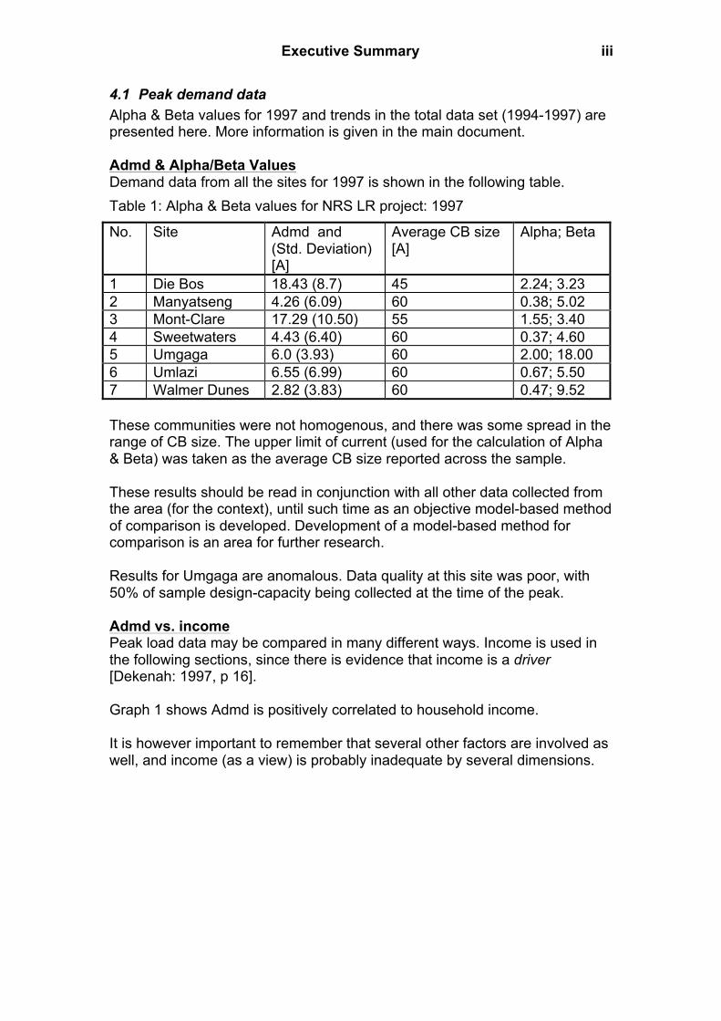
4.1 Peak demand data Alpha & Beta values for 1997 and trends in the total data set (1994-1997) are

presented here. More information is given in the main document. Admd & Alpha/Beta Values Demand data from all the sites for 1997 is shown in the following table. Table 1: Alpha & Beta values for NRS LR project: 1997

No. Site Admd and (Std. Deviation) [A]

Average CB size [A]

Alpha; Beta

1 Die Bos 18.43 (8.7) 45 2.24; 3.23 2 Manyatseng 4.26 (6.09) 60 0.38; 5.02 3 Mont-Clare 17.29 (10.50) 55 1.55; 3.40 4 Sweetwaters 4.43 (6.40) 60 0.37; 4.60 5 Umgaga 6.0 (3.93) 60 2.00; 18.00 6 Umlazi 6.55 (6.99) 60 0.67; 5.50 7 Walmer Dunes 2.82 (3.83) 60 0.47; 9.52 These communities were not homogenous, and there was some spread in the

range of CB size. The upper limit of current (used for the calculation of Alpha & Beta) was taken as the average CB size reported across the sample.

These results should be read in conjunction with all other data collected from

the area (for the context), until such time as an objective model-based method of comparison is developed. Development of a model-based method for comparison is an area for further research.

Results for Umgaga are anomalous. Data quality at this site was poor, with

50% of sample design-capacity being collected at the time of the peak. Admd vs. income Peak load data may be compared in many different ways. Income is used in

the following sections, since there is evidence that income is a driver [Dekenah: 1997, p 16].

Graph 1 shows Admd is positively correlated to household income. It is however important to remember that several other factors are involved as

well, and income (as a view) is probably inadequate by several dimensions.

Executive Summary iv

0

2

4

6

8

10

12

14

16

18

20

0 1000 2000 3000 4000 5000 6000

Average income [R/Household/Month]

Adm

d [A

]

Graph 1: Admd vs. Income (1994-1997) Coefficient of variation vs. income Coefficient of variation is an essential component to calculation of Alpha and

Beta parameters used in estimation of design-voltage-drop. A definition of coefficient of variation is included in the main body of the document.

Coefficient of variation is plotted against mean monthly household income in Graph 2.

0.00

0.20

0.40

0.60

0.80

1.00

1.20

1.40

1.60

1.80

0 1000 2000 3000 4000 5000 6000


Coef

ficie

nt o

f Var

iatio

n [A

/A]

Graph 2: Coefficient of variation vs. Average household income (1994-1997) There appears to be a negative correlation between coefficient of variation

and mean household income. Poorer communities have higher coefficients of variance. This implies that special precautions must be taken when designing for poor communities, particularly where a small quantity of consumers is involved.

Executive Summary v

4.2 Socio-demographic data A socio-demographic questionnaire was implemented as a standard, at 90%

of houses being monitored, throughout all of the projects. Enough socio-demographic data has been collected to develop a description

of these consumers for reference purposes (in order to fix the context under which load readings are compared) as well as for model-building purposes.

An detailed pro-forma analysis of this information is included in the

appendices, with a synopsis.

5. SPECIFIC PROBLEMS REQUIRING CORRECTION Several problems were identified during this project which require correction.

5.1 Management of loggers by DCO’s Management of data loggers and data collection by DCO’s was sometimes

poor and this led to loss of data. Most faults were soluble by training. There is a great need for intuitive downloading software.

5.2 Faults on TRI loggers Two new faults were identified on TRI data loggers. Data loggers at Manyatseng, Umlazi and Umgaga are affected. Software diagnostic techniques have been developed which deal with these

problems.

5.3 Data quality & data analysis The data collection projects were compressed this year, due to funding

problems. In most projects, data collection was established shortly before winter 1997. Thus follow-on energy-related studies from data collected in 1997 are

probably not viable using this data. This is a great loss.

5.4 Project scope It was originally envisaged in late 1996 that it may be possible to carry out

bulk-monitoring at the project sites (i.e. sending-end voltage and load). This proved to be impossible under the following constraints:

• Project funding • Support required from DCO’s • Development of methodology & training • Development of database infrastructure and analysis techniques • Advanced documentation required from site

Such extensions to the project would require a lead-time of about 6 months to implement and should be budgeted.

Executive Summary vi

6. REPORTING & DISSEMINATION OF RESULTS There are many stake-holders in this project. Several types of reporting have

been carried out or are planned:

Reports • Progress reports to NRS 034 WG • Progress reports to Eskom TRI • Feedback to DCO’s

Publications & Training

• A programme of publications is in place and two papers have been presented in 1997.

• DCO-Training workshop is planned for late November 1997 Dissemination of data

• Extracts of data have been disseminated to ESKOM DT and to NRS 034 WG

• Extracts of data are published on ESKOM NRS-Project WWW internet site.

7. COST/BENEFIT ANALYSIS Cost The cost of maintaining this project is in the region of R 423,000/annum

(approximately R60,500/project/annum). This includes:

• Capital to establish at least one new site each year. • Project management • Project consultants • Software development • Market research surveys

Benefit The results of this project continue to support design-guidelines in the region

of 0.6-0.9 kVA for poor communities. Other benefits may be expected:

• Calibration of demand-prediction tools • Decision-support for QOS standards development • Increased LR cost-effectiveness • Decision-support for circuit-breaker based load-limiting • Outputs from academic collaboration

Executive Summary vii

8. ESKOM PERSPECTIVE Eskom electrifies consumers in a process which requires an investment and is

constrained by several factors such as legislation (covering safety and QOS) and availability of funding.

The investment is recovered by revenue from sale of electricity. In this process it is important to be able to manage:

• The meeting of QOS obligations • Cost-effects of QOS constraints on capital investment • Consumer-supplier relationships • The Marketing-sales relationship

The NRS LR project provides information which will impact in most of these areas at a rather fundamental level.

Executive Summary viii

9. RECOMMENDATIONS Recommendations are drawn from discussion of results and specific problems

sections.

9.1 Improve data verification More work on data-verification is still required to isolate errors in source data if

at all possible, and ensure that analysis of data is more robust and less labour intensive.

This work should be completed before the next cycle of data analysis. This is an area which must be addressed early in the next phase of the project

by the project manager and the software developer.

9.2 Modify logger downloading software Quality of software for logger downloading must be upgraded as a matter of

urgency. An intuitive interface is required to avoid the potential spoilage of data.

The work should be completed in time to affect the next phase of the LR

project.

9.3 Implement postal-warning for market research work in “rich” areas Postal warnings should be distributed by the DCO’s about 2 weeks prior to

M.R. surveys in affluent areas. This should significantly increase the yield of sociometric data from these

areas to the 90 %-of-logged level.

9.4 Apply DCO training course Intensive training of data-collectors (and their managers) is required. A workshop planned for 26 November 1997 will go some way towards solving

this problem. Collectors and managers from DCO’s must be urged to attend.

9.5 Review project cycle The current project schedule caused predictable difficulties with this phase of

the project. Most activities were highly compressed. This led to a reduction in the quality of data collected.

There is a great need to extend the planning horizon on this project, since

municipalities are not necessarily able to react according to the needs of TRI’s project-management cycle.

Most DCO’s need planning information each year in November in order to

react suitably for the following winter peak. This is an eight-month lead-time.

Executive Summary ix

9.6 Review project portfolio Three projects will be free by the end of 1997, and data-logging equipment

will be available for movement to other NRS LR project sites. These sites must be nominated and decided by December 1997, so that

movement can take place on a rational basis for 1998. ESKOM TRI have indicated a need to extend the project to encompass bulk

feeder monitoring & sending-end voltage monitoring. Under these circumstances the project portfolio should be carefully chosen to

remain relevant to both ESKOM and the DCO’s, (who both invested in this project), whilst satisfying the needs of NRS 034, and collating data of sufficient quality to warrant academic involvement.

9.7 Review sampling technique The sample design-criteria for measurement precision of the Admd is too

large. It “swamps” temperature-sensitivity and load-growth indices, and plainly

results in rather loose measurement of certain sociodemographic factors which are important for demand prediction.

Sampling strategy must be reviewed before the 1998 phase of this project. An “uncertainty budget” approach must be applied and managed. The work must be undertaken by the statistics consultant and reviewed by the

project team.

9.8 Support processes to beneficiate data We now have a significant body of standardised data. This author is of the conviction that the benefits of this body of data are not yet

realised. Stimulation of follow-on academic research is required to address them.

1

1. INTRODUCTION This report describes the results of a project initiated to collect electrical-load and socio-demographic data from domestic consumers in townships. Some preliminary analysis of data has been carried out and is presented. Data from the database has been provided to academic researchers. Extracts from the database have been provided to NRS 034 working group and to ESKOM DT. The results of this project are important to electrification planners, since they indicate appropriate levels of supply, and support initiatives towards design levels in the region of 0.6-0.9 kVA. Results will continue to impact upon policy formulation in electrification, particularly in terms of design-level and quality of supply. Data were collected from 7 distinct projects in 1997, which now form part of a “library” of 13 case-studies collected in a similar manner over the period 1994-1997. The project was placed under considerable stress this year, because no funding was available to carry out project management until mid-March 1997. Consequently data-collecting partners (municipalities, universities & Eskom) struggled to establish their projects smoothly by winter 1997. Data quality at most sites was affected in some way.

2. AIM OF RESEARCH PROJECT The primary aim of this project is to gather data so that electrification parameters may be supplied to NRS034 working group for inclusion in guidelines on reticulation design. Secondary aims are to facilitate follow-on research by academic institutions, and also to disseminate results of this project. This aim was achieved in 1997.

2

3. RESEARCH PROCESS The research method involved a number of tasks, some direct and others overhead-related.

3.1 Summary of method A typical township collection project involves the following: • Data loggers belonging to the DCO or to the NRS LR project are installed in a township • Data is downloaded monthly by the DCO and forwarded to the project manager for analysis and

reporting • A data logger should operate continuously in position for a period of two years • Sociometric data are collected from each household logged, in the winter of each year and

forwarded to the project manager for analysis & reporting In total, seven such projects were controlled during 1997.

3.2 Research tasks The research process involved the following tasks during this project year: A: Data collection activities: DCO’s & Loggers • Manage load research projects in progress at data-collecting organisations • Purchase & distribute data-logger equipment to Data Collecting Organisations (DCO’s) • Revise project documentation (manual, questionnaire etc.), based upon learning. B: Market research • Manage market-research. C: Data collation • Store data onto database • Specify, subcontract & test modifications to NRS LR database software • Review data quality. • Facilitate parallel research-studies by academia. D: Data analysis • Contract statistical analysis of data collected in 1997. E: Identification & correction of problems F: Reporting & dissemination of results • Report progress & results to ESKOM TRI & NRS • Report to TRI, DCO’s, and NRS 034 Working Group (WG) • Lead Load data collection workshop in preparation for the 1998 project • Report on and publicise the NRS LR project initiative

3

4. RESULTS Useful data have been collected from all 7 sites during 1997. A data quality problem was experienced at Umgaga in Durban, where winter was recorded from only 30 consumers, about half the design value. A summary of all data for each township is included in the appendices. All analysis contained in the following sections was carried out by the author.

4.1 Nature & volume of data Several types of data were collected onto the data-base for each case study: • A township-level questionnaire • A sociodemographic questionnaire at each household • Load data at each household • Hourly air-temperature data for the area. A summary of data collected in 1997 is given in the table below. Table 1: Summary of data collected in 1997 Data type Volume of data

collected Comment

Load-data 26 M readings

Date & time stamped current and voltage. Each project is organised as a group of database tables, with one table per data-logger. About 651 MB of load data was collected to September 1997. Present size of all load data is 1689 MB.

Air temperature data

53 k readings

Hourly air temperature collected from adjacent weather office, and stored as text files. Air-temp data has been collected for all project sites since 1994. Present size of all air-temp data is 1.8 MB.

Sociometric questionnaires

456 questionnaires (91% recovery)

All sociometric forms collected and entered onto database. Present size of all sociometric tables is 1.2 MB.

4

4.2 Summary of 1997 load data per township Summarised load-data are presented in the following tables which cover logging information, and data about the coincident peaks. Logging information A summary of logging information is shown in table 2. Table 2: Summary of logging information : 1997 NO. PROJECT NAME D.C.O. NO. OF

LOGGERS NO. LOGGER CHANNELS

PROJECT START

1 Die Bos Strand, W. Cape

Helderberg/Gibb 10 61 Jul 1997

2 Manyatseng Ladybrand, F.S.

ESKOM: Bloemfontein

19 72 Nov 1997*

3 Mont Clare Johannesburg, G.T.

Johannesburg GMTC

17 79 Nov 1996*

4 Sweetwaters Pietermaritzberg, Natal

Pietermaritzberg electricity

19 72 May 1997*

5 Umgaga Durban, Natal

Durban Corp. 16 66 Apr 1997

6 Umlazi Durban, Natal

Durban Corp. 13 72 Mar 1997*

7 Walmer dunes Port Elizabeth, E. Cape

Port Elizabeth Electricity

12 80 May 1997

* = projects which continued from 1996. Four projects were a continuation from 1996. Three projects were newly established in 1997. More information regarding project duration, magnitude of data collected, quality measures and specific site information is provided in appendix A. Peak data The five highest peaks for each township were registered, along with their date and time. This data is shown in table 3. Other information is also given : • Total scalar current for all of the logger channels (I tot) • Number of active channels counted at this time (N) • Average current per channel at the time of this peak (I ave) • Standard deviation of the currents at the time of this peak (Std dev)

5

Table 3: Results of NRS LR Project : 1997

PROJECT PEAK DATA 1 Die Bos

Strand, W. Cape Peak no. Date Itot [A] N I ave[A] Std Dev [A]

1 13/8/97 19:15 1124 61 18.43 8.70 2 7/8/97 19:40 1040 61 17.05 10.30 3 19/8/97 19:40 976.2 61 16.00 10.27 4 6/8/97 19:10 919.1 54 17.02 12.70 5 21/8/97 19:30 912.3 61 14.96 10.32

2 Manyatseng Ladybrand, F.S.

Peak no. Date Itot [A] N I ave[A] Std Dev [A]

1 15/7/97 19:40 285.2 67 4.26 6.09 2 16/7/97 19:00 273.3 67 4.08 5.08 3 2/6/97 20:20 265.5 68 3.90 5.68 4 10/6/97 19:25 265.4 68 3.90 5.12 5 16/6/97 18:25 258.1 72 3.58 4.41

3 Mont Clare Johannesburg, G.T.


1 30/6/97 20:00 1366 79 17.29 10.50 2 9/7/97 18:55 1328 75 17.71 10.35 3 1/7/97 18:40 1283 79 16.24 11.77 4 2/7/97 19:30 1234 79 15.62 11.22 5 7/7/97 18:15 1227 75 16.36 11.85

4 Sweetwaters Pietermaritzberg, Natal


1 2/6/97 18:00 301 68 4.43 No reading 2 19/6/97 17:50 296.8 68 4.36 5.13 3 8/7/97 19:10 291.4 68 4.29 6.40 4 13/6/97 17:40 287.2 68 4.22 6.39 5 20/6/97 16:20 282.5 68 4.15 2.92

6

Project (Contd.) PEAK DATA (Contd.) 5 Umgaga

Durban, Natal Peak no. Date Itot [A] N I ave[A] Std Dev [A]

1 21/8/97 18:50 174 29 6.00 3.93 2 16/8/97 18:25 165.1 29 5.69 4.42 3 11/8/97 18:10 156.7 29 5.40 4.53 4 13/5/97 19:15 155.5 33 4.71 4.97 5 15/8/97 18:50 153.5 29 5.29 5.07

6 Umlazi Durban, Natal


1 23/5/97 17:40 393.1 60 6.55 6.99 2 29/5/97 18:40 387.9 60 6.47 6.27 3 2/6/97 17:45 360.7 60 6.01 6.09 4 8/6/97 17:55 357.9 60 5.97 5.06 5 28/6/97 18:20 354.3 60 5.91 5.14

7 Walmer dunes Port Elizabeth, E. Cape


1 29/6/97 19:40 200.2 71 2.82 3.83 2 25/7/97 19:30 200 71 2.82 3.74 3 18/7/97 19:05 198.7 71 2.80 4.91 4 2/6/97 19:25 198.6 71 2.80 3.44 5 13/6/97 18:55 193.3 71 2.72 4.25

The most appropriate method for depiction of representative peaks is an area requiring further study. All load data results should be read in conjunction with all other data collected from the area (for the context) until such time as an objective model-based method of comparison is developed. Development of a model-based method for comparison between different community types is an area for further research.

4.3 Summary of 1997 sociometric data per township This section presents a short breakdown of the full socio-demographic pro-forma analysis presented in the Appendices. The aim of these synopses is to supply enough information to allow a township to be assessed in terms of these criteria, preferably without having to survey the dwelling internally. For this purpose, ownership of television sets(i.e. for aerials) is quoted.

4.3.1 Site synopsis: Die Bos, Strand, Cape Town This is a very wealthy suburb.

7

Very few households reported earning less than R4000/hh/month, in a well serviced area with tarred roads. The site is close to a major centre. There is 100 % ownership of most appliances, except for hotplates, which are not owned at all. Built area of the houses is in the region of 180 m2 . Consumers are not happy with their supply and 60% of households report one or more problems. Current limiting of 30A is applied to most of the customers, but can be lifted under new tariffs.

4.3.2 Site synopsis: Manyatseng, Ladybrand This site has high electrification, and tarred main roads (secondary lanes between houses are gravel) This site is more than 100km from a city. Water is supplied mostly to taps in the yard, and only 14% have water piped into the house. Inhabitants are poor(R1071.00/household/month), and earn about the national average per house1. Ownership of water geysers is very low, and just over half own a television set. Three quarters of the inhabitants own their dwellings, and built area of the houses is of the order of 50m2. There is a wide variety of building materials in use. About half of the roofs are either asbestos or tin, and walls are chiefly brick or concrete-block, (30-40%) followed by tin (17%). Use of alternative fuels is high , and this appears to be part of the lifestyle. This site can get very cold in winter.

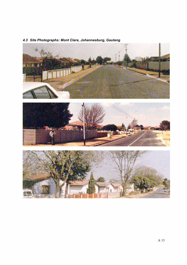
4.3.3 Site synopsis: Mont-Clare/Claremont, Johanneburg This site features high % electrification, in a well-serviced environment with piped water, water-borne sewerage & tarred roads. The site is close to a major centre. Inhabitants are relatively wealthy (income of R3221/month/house, which is more than 3 times the national average ) and generally own their houses. All houses electrified have hot-water geysers, and 95% own a television. Built area of the houses generally cover 90m2. These houses have mostly brick walls and corrugated iron roofs. Very little alternative fuels are used.

8

4.3.4 Site synopsis: Sweetwaters, Pietermaritzberg The site is within 8 km of a major centre. Inhabitants are as wealthy as the national average, and own their own buildings. About half of the population own a television set, and there are no geysers. Built-area of the houses is in the region of 50m2 . Most houses have tin roofs. Most walls are of mud (77%) or concrete block (10%). Over half the respondents use paraffin.

4.3.5 Site Synopsis: Umgaga, Durban About half of the stands are electrified. This site features high-density living on a steep slope. Plots are small with few formal boundaries. Internal roads are ummade. The site is 35 km from a city centre. Inhabitants earn about R1200/hh/month, the national average income. Ownership of dwellings is high. Water is obtained from nearby communal taps. About half of the households have a TV set. Most dwellings have tin roofs and clay/mud walls. The climate is moderate, and portion of the sample uses any alternate fuel source (paraffin at 36%) Consumers are happy with their supply.

4.3.6 Site Synopsis: Umlazi, Durban This site features high electrification (90%), in an area with 100% tarred roads. The site is 20km away from a city center. Inhabitants earn twice the national average and are thus relatively wealthy. Ownership of buildings is high. Most houses have piped water, but geyser ownership is low at 10%. 80% of houses have a TV. Built area of the houses is about 50m2, and most houses have asbestos roofs(90%) and brick walls (90%). The climate is moderate, and only small portion of the sample uses any alternate fuel source (paraffin at 25%) Consumers are unhappy with their supply.

4.3.7 Site Synopsis: Walmer location, Port Elizabeth This site features 50% electrification, in an area where only arterial roads are tarred.

9

The area is 7 km from a city centre. Inhabitants are 20 % poorer than the national average. Water is obtained from a tap in the yard, and most houses are completely built from corrugated iron. About 50% of households have a TV. The climate is moderate here, and alternative fuels are not used much. 40% report using paraffin. Consumers are happy with their QOS.

4.4 Air temperatures The following table gives a break-down of temperature information for the sites: Table 4: Air temperature data: -All sites winter 1997. No. Site Climatic region Average daily temperature in

July2 (and average of daily minima)

1 Die Bos, Strand, Cape Town

Mediterranean 12.6§C (7.2§C)

2 Manyatseng, Ladybrand, Free State

Temperate sub-tropical 6.7§C (-2.4§C)

3 Mont Clare, Johannesburg, Gauteng

Temperate sub-tropical 9.7§C (4.2§C)

4 Sweetwaters, Pietermaritsberg, Natal

Humid sub-tropical 12.9§C (6.4§C)

5&6 Umlazi & Umgaga, Durban, Natal

Humid sub-tropical 16.5§C (11.7§C)

7 Walmer Dunes, Port Elizabeth, E. Cape

Temperate sub-tropical (Coast)

13.4§C (8.2§C)

The average daily temperature over July month is quoted because: • Other studies have displayed a domestic sensitivity to demand (at the peak) of about 2 % per §C

[Dekenah: 1997, p6] 3. • The information is easily available4.

10

5. DISCUSSION OF RESULTS All analysis contained in the following sections was carried out by the author.

5.1 Alpha/Beta values for 1997 data set Table 5: Alpha & Beta values for NRS LR project: 1997 No. Site Admd (Std Deviation)

[A] Average CB size [A]

Alpha; Beta

1 Die Bos 18.43 (8.7) 45 2.24; 3.23 2 Manyatseng 4.26 (6.09) 60 0.38; 5.02 3 Mont-Clare 17.29 (10.50) 55 1.55; 3.40 4 Sweetwaters 4.43 (6.40) 60 0.37; 4.60 5 Umgaga 6.0 (3.93) 60 2.00; 18.00 6 Umlazi 6.55 (6.99) 60 0.67; 5.50 7 Walmer Dunes 2.82 (3.83) 60 0.47; 9.52 These communities were not homogenous, and there was some spread in the range of CB size. The upper limit of current used for the calculation of Alpha & Beta was taken as the average CB size reported across the sample. The actual value of CB which should be used for this calculation (i.e. mean, median etc.) is an area for further research. Results for Umgaga are anomalous. Data quality at this site was poor, with 50% of sample design-capacity being collected at the time of the peak (see table 3).

5.2 Trends in data set 1994-1997 Several trends have become apparent over the four consecutive years of this project. Data is drawn from the current period of study, and from the most recent DMEA report on this project [Dekenah: 1997] which presents data from all of the previous periods.

11

This total body of information is shown in the table below: Table 6: Total body of data 1994-1997 Serial Township

Name Year

Time electrified [Yr.]

CB size [A]

Income [R/hh/Month]

Mean daily air-temp [July][øC]

Admd [A]

C.V. [A/A]

1 Cloetesville ‘95 10 60 3100 11.2 14.5 0.49 2 Die Bos ‘97 >10 44 6000 13 18.4 0.47 3 Kwazakhele ‘96 3 80 1000 12.5 4.1 1.24 4 Manyatseng ‘96 3 900 6.7 3.8 1.1 5 Manyatseng ‘97 6 60 1080 6.2 4.26 1.43 7 Mont Clare ‘96 5 3200 8.4 16.8 0.64 6 Mont Clare ‘97 6 55 3600 9.7 17.29 0.61 8 Sweetwaters ‘96 1 700 11.2 4.1 1.73 9 Sweetwaters ‘97 6 60 1200 13 4.43 1.16 10 Umgaga ‘97 4 60 1200 16.5 6 0.66 11 Umlazi ‘96 6 2500 15.4 3.2 0.91 12 Umlazi ‘97 7 60 1900 16.5 6.55 1.07 13 Walmer ‘97 3 60 900 13 2.82 1.36 The table shows 13 data collection projects, arranged alphabetically. Projects 4 & 5, 6 & 7, 8 & 9, and 11 & 12 are drawn from consecutive years at the same site. All projects from the current year of study are shown shaded. “Time since electrified” shows some anomalies for projects running in consecutive years, in Sweetwaters and Manyatseng. This is an area for further research. This peak load data may be compared in many different ways. Income is used in the following sections, since there is evidence that income is a driver [Dekenah: 1997, p 16]. It is however important to remember several other factors are also involved, and income(as a view) is probably inadequate by several dimensions.

12

5.2.1 Admd vs. Income

0

2

4

6

8

10

12

14

16

18

20

0 1000 2000 3000 4000 5000 6000


Adm

d [A

]

Graph 1: Admd vs. Income The trend of Admd vs. Income is positive and appears to saturate. Round data points indicate reported time-since electrified values of 4 years and less. Unfortunately these are probably too closely clustered to draw any useful inferences. Triangular data-markers indicate an average stated time-since-electrified of 5 years and above. The point on the extreme right of the graph is Die Bos, which appears to have saturated. The exact value of income is not known for this site. However we do know that it is at least R4000, the lower bound stated by the respondents. The saturation displayed here may also be a result of demand -limiting by customer circuit-breakers. A more intensive study of load data collected from such restricted consumers is an area for further research.

5.2.2 Coefficient-of-variation vs. Income Coefficient of variation is an essential component to calculation of Alpha and Beta parameters used in estimation of design-voltage-drop. Coefficient of variation is the ratio of the standard deviation to the mean, at the time of peak load as shown in equation 1.

Equation 1 This is the inverse of slenderness ratio S 5. The following graph shows the trend of coefficient of variation against income. Circular data points on the graph indicate a reported time-since-electrified of 4 years and less. Square data-markers indicate an average stated time-since-electrified of 5 years and above.

13

0.00

0.20

0.40

0.60

0.80

1.00

1.20

1.40

1.60

1.80

0 1000 2000 3000 4000 5000 6000


Coef

ficie

nt o

f Var

iatio

n [A

/A]

Graph 2: Coefficient of variation vs. Income There appears to be a negative correlation between covariance and mean household income. Poorer communities have higher coefficients of variance. This means special precautions must be taken when designing for this area, particularly where small numbers of consumers are concerned. This relationship is beginning to be better-defined for urban dwellers. The effects of “ruralisation” have not yet been established and are an area for further study.

5.2.3 Load growth Growth in registered peaks for the four townships which have been monitored over a two-year period are shown below: Table 7: Growth in registered peak Township Period Growth [p.u.] Manyatseng 96/7 1.12 Mont Clare 96/7 1.03 Sweetwaters 96/7 1.08 Umlazi 96/7 2.05 The figure for Umlazi is misleading and casts doubts on the handling of data over the 1996 period, where this data were pre-processed by the DCO. Based upon the information supplied in the coefficient of variation profile however, the error was probably systematic. The sample design for these areas was guided by a need to determine the peak load with a sample error within ñ1 A at 90 % confidence. This criteria has the potential to obscure assessment of load growth over two consecutive years, since an error of 1 A may constitute a 20 % movement in either the numerator or denominator of a per-unit calculation. Such uncertainties would be resolved by a larger sample size.

14

5.2.4 Comment on temperature sensitivity Inspection of table 6 shows no obvious signs of sensitivity (to average daily temperature) amongst consecutive years. This is not suprising for the following reasons: • The peak event is an extreme and has an associated error • Temperature sensitivity is likely to be smaller than this error Extraction of air temperature sensitivity from the current database is an area for further research. Hourly air temperature data has been collected for the entire period, for all projects.

5.2.5 Comment on quality of market research work All market research was carried out “blind” (the contractor did not know what results to expect). Market research has assessed the mean income level, year-on-year as shown by the table below: Table 8: Year-on year assessment of income (same sample) Township 1996/1997 Income pu growth Manyatseng 905 to 1071 1.18 Mont-Clare 3221 to 3607 1.12 Sweetwaters 731 to 1204 1.64 Umlazi 2480 to 1869 0.753** The Sweetwaters and Umlazi entries appear to be flawed. Umlazi, (**) becomes part of the trend line on the Admd/Income graph in 1997 (the sample size for Umlazi approximately doubled in 1997, to 60 consumers). Sampling would account for a significant portion of this error. In general, the standard deviation of incomes is almost equal to the mean income at the R 1000/hh/month level. Thus a 90% confidence interval is ñ R 200/hh/month, roughly 20% of the range. Such uncertainties would be resolved by adoption of a larger sample size.

5.3 Effects of current-limiting on Admd (Die Bos) The load at Die Bos appears to have been depressed, despite high wealth-levels and long time-with electricity. This may be due to the effect of circuit breaker limiting applied. The median CB size in this area is 35A, with the mean at 45 Amp. However, the distribution of currents at the time of peak is in the region of 18 A, approximately half way between the constraints of zero and the CB limit. Results from this site are an extremely important indicator of effects of load-limiting on wealthy consumers. At this level, a significant portion of the population experience the limiting. Analysis of the sociodemographic survey shows that 50 % of this sample noted that “the CB tripped” and that “electricity goes off often”. This is an area for further research, since the client has started to define “acceptable” QOS based upon his perceptions.

15

6. SPECIFIC PROBLEMS REQUIRING CORRECTION

6.1 Management of loggers by DCO’s Several aspects of project, logger and data management by DCO’s need to be addressed.

6.1.1 Corruption of data by DCO’s It has been noted that in some cases, data handling by DCO’s is poor and users have corrupted source load data. Typically this happens when the user applies his own spreadsheet package to view the data, and then saves it in the proprietary format, a process that confounds efforts to automate file-handling, interpretation and analysis. There are a huge amount of possible formats available, and the proprietary Dataview package was specifically developed and distributed to get around this problem. Instruction is required here.

6.1.2 Memory clearing during data-logger download Logger data memory is not always cleared after a logger download. Downloading data is a very repetitive process which requires one to work systematically, often with distractions. This problem would be solved by better downloading software, which must be developed. The TRI data loggers are the current project standard, and so any application would be designed around this.

6.1.3 Time-synchronisation of data-loggers There is a facility to correct the logger’s real time clock at each downloading, having corrected the time-clock on the download-computer. Error may arise from not synchronising the logger clock to the computer, or supplying a wrong time to the computer. Incorrectly synchronised data loggers generally lead to loss of some data. Very often it is only possible to confirm time-synchronisation by inspection of general power-failure events. This problem could be partially solved by better downloading software, and training.

6.1.4 Review of collected data by DCO DCO’s do not appear to have reviewed their own data after each download. This is an important part of the feedback process, and special software (DATAVIEW) was developed to enable this. Training is indicated.

6.1.5 Repair of data loggers In some cases, obviously faulty data loggers have not been repaired, leading to a steady decline in collection efficiency. It is currently the responsibility of the DCO’s to maintain their logging capability. This entails arrangements, repair and payments. This appears to have happened at the Umgaga site.

16

6.2 Faults on TRI data-loggers Two new faults were noted on TRI data loggers during 1997.

6.2.1 Data repetition/skipping Data-loggers at Manyatseng are not downloading properly. In any file, two typical types of error are encountered simultaneously. -during downloading, the loggers download a particular day several times -other days are missed. The problem has been noted in older loggers, with 64 kB memory capacities only, and is being taken up with the suppliers. Manyatseng is currently the only site working with 64 kB data loggers. This problem is very difficult to isolate using a spreadsheet, but leads to “key violations” when inserting the data into a database, which only accepts a particular data reading (i.e. at that time & date) once. Analysis procedures using less stringent criteria will most probably supply incorrect analysis results due to this fault. In addition, data will never be time-synchronised.

6.2.2 Channel failure : high indicated current It has been noted on several occasions that channel 4 of a TRI logger will fail to a constant load in the region of 100A. This hardware fault severely distorts any attempts at analysis which are not “aware” of the problem. The problem may be identified by a plot of standard deviation vs. time which is large and fairly constant.

6.3 Data quality & data analysis The compressed nature of the project meant that many DCO’s were essentially establishing their projects during winter 1997, at which stage projects happened to be sufficient. The usefulness of data collected in this manner is limited to demand-only studies. Energy-related studies have to be adjusted to account for sparsity of data. This introduces a significant analysis overhead for any follow-on research work and should be avoided.

6.4 Project scope It was originally envisaged in late 1996 that it may be possible to facilitate bulk-monitoring at all the project sites. This proved to be impossible under the following constraints: • Project funding • Support required from DCO’s • Development of methodology & training • Development of database infrastructure and analysis techniques • Advanced documentation of site Such extensions to the project would require a lead-time of at least 6 months to implement and should be budgeted.

17

7. REPORTING AND DISSEMINATION OF RESULTS Several types of reporting have taken place during this project.

7.1 Reporting Technical and progress reports have been submitted to the following: • NRS working group at each meeting through the year. • Project leader, ESKOM TRI, through the year. This report is the final reporting output from this project in 1997.

7.2 Dissemination of data Raw load data : Raw load data has been distributed to the following organisations on CD ROM: • 2 M.Sc. Eng. projects, University of Stellenbosch • 2 M.Sc. Eng. projects, University of Cape Town Work is presently focused on assessment of design risk, estimation of transmission losses and related areas. Design-information: • Extracts of data have been disseminated to ESKOM DT and to NRS 034 working group. • Case-studies of LR work have been posted on the ESKOM Internet web-site for public access6.

7.3 Publications presented/ in progress An active publication programme is in place. Two papers are in preparation, and a large number are envisaged for exposure in 1998. Papers presented: 1. Dekenah M, Herman R, Gaunt C T, “Results from the NRS load research project: Implications

for management of domestic QOS”, Applitech, 1997. 2. Dekenah M, Herman R, Gaunt, C T “Application of load data for design and metering of electrical

distribution networks”, ETAM , October 1997. Papers in preparation: 1. Series of 8 short articles for insertion into ELEKTRON, under leadership of Dr. R Herman. 2. Dekenah M and Gaunt CT “ Parameters for electrification”, for presentation at DUEE, Cape town,

1998. 3. Dekenah M, Herman R and Gaunt C T “Collection of load data from domestic consumers”, for

presentation at DUEE, Cape town , 1998. 4. Lawrence V and Dekenah M “Demand and restricted domestic consumers” for submission to

SAIEE transactions. There are several other publications are in progress in related areas by the academic partners.

7.4 Training workshop A training workshop has been arranged for 26th November. It will be led by the author, and will strive to reduce training weaknesses experienced over the past year of the NRS LR programme.

18

8. COST/BENEFIT ANALYSIS Cost The cost of maintaining this project is in the region of R 423,000/annum (approximately R60,500/project/annum). This includes: • Capital required to establish at least one new site each year. • Project management. • Project consultants. • Software development. • Market research surveys. Benefit The results of this project continue to support design-guidelines in the region of 0.6-0.9 kVA for poor communities. This amounts to a substantial return on investment. Other benefits may be expected: • Closed-loop calibration of demand-prediction tools. • Decision-support for QOS standards development. • Leading-edge outputs from academic collaboration. • Increased LR cost-effectiveness.

19

9. RECOMMENDATIONS Recommendations are drawn from discussion of results and specific problems sections.

9.1 Improve Data verification More work on data-verification is still required to isolate errors in source data if at all possible, and ensure that analysis of data is more robust and less labour intensive. This work should be completed before the next cycle of data analysis. This is an area which must be addressed early in the next phase of the project by the project manager and the software developer.

9.2 Modify logger downloading software Quality of software for logger downloading must be upgraded as a matter of urgency. An intuitive interface is required to avoid the potential spoilage of data. The work should be completed in time to affect the next phase of the LR project.

9.3 Implement postal warning for market research work in “rich” areas Postal warnings should be distributed by the DCO’s about 2 weeks prior to M.R. surveys in affluent areas. This should significantly increase the yield of sociometric data from these areas to the 90 %-of-logged level.

9.4 Apply DCO training course Serious training of data-collectors (and their managers) is required. A workshop planned for 26 November 1997 will go some way towards solving this problem. Collectors and managers from DCO’s must be urged to attend.

9.5 Review project cycle The current project schedule caused predictable difficulties with this phase of the project. Most activities were highly compressed. This led to a reduction in the quality of data collected. There is a great need to extend the planning horizon on this project, since municipalities are not necessarily able to react according to the needs of TRI’s project-management cycle. Most DCO’s need planning information each year in November in order to react suitably for the following winter peak. This is an eight-month lead-time.

9.6 Review project portfolio Three projects will be free by the end of 1997, and data-logging equipment will be available for movement to other NRS LR project sites. These sites must be nominated and decided by December 1997, so that movement can take place on a rational basis for 1998.

20

ESKOM TRI have indicated a need to extend the project to encompass bulk-monitoring and sending-end voltage monitoring. Under these circumstances the project portfolio should be carefully chosen to remain relevant to both ESKOM and the DCO’s, (who have both invested in this project), whilst satisfying the needs of NRS 034, and collating data of sufficient quality to warrant academic involvement.

9.7 Review sampling technique The sample design-criteria for measurement precision of the Admd is too large. It “swamps” temperature-sensitivity and load-growth indices, and plainly results in rather loose measurement of certain sociodemographic factors which are important for demand prediction. Sampling strategy must be reviewed before the 1998 phase of this project. An “uncertainty budget” approach must be applied and uncertainty managed. The work must be undertaken by the statistics-consultant and reviewed by the project team.

9.8 Support processes to beneficiate data We now have a significant body of standardised data. This author is of the conviction that the benefits of this body of data are not yet realised. Stimulation of follow-on academic research is required to address them.

21

10. ACKNOWLEDGMENTS The assistance and cooperation of the following organisations is gratefully acknowledged. ESKOM TRI NRS 034 working group Durban Corporation ESKOM : Bloemfontein distributor Pietermaritzberg Electricity Johannesburg GMTC Helderberg GMTC Port Elizabeth Electricity University of Stellenbosch Consumer Link Africa TLC Software Gibb Africa REFERENCES: 1 All Media & Product Survey, (AMPS) 1995. 2 Data source: Climate enquiries, SA Weather bureau, Pretoria. 3 Dekenah, M. “The NRS National Load Research Project: 1994-1996”, Project EL 9404, Dept Min. & Energy Affairs, March 1997. 4 Macmillan New Secondary schools atlas for SA, Macmillan, 1996, p23. 5 Gaunt, C.T. “Implications of planning and design decisions in electricity distribution”, 12th AMEU Technical meeting, Potchefstroom, 1988. 6 NRS LR Project World-Wide Web address: www.eskom.co.za/graphics/esi/eskom/nrs/nrslrp.htm

APPENDIX A

Summary township data

Appendix A: Contents 1. INTRODUCTION ............................................................................................................................................. 1

1.1 SITE SYNOPSIS .................................................................................................................................................... 1 1.2 SITE PHOTOGRAPH .............................................................................................................................................. 1 1.3 LOAD DATA ........................................................................................................................................................ 1 1.4 SOCIO-DEMOGRAPHIC SUMMARY ....................................................................................................................... 1

2. DIE BOS, STRAND, CAPE .............................................................................................................................. 2

2.1 SITE SYNOPSIS: DIE BOS ..................................................................................................................................... 2 2.2 LOAD DATA: DIE BOS ......................................................................................................................................... 2 2.3 SITE PHOTOGRAPHS: DIE BOS, STRAND, CAPE TOWN ........................................................................................ 3 2.4 SOCIO-DEMOGRAPHIC SUMMARY : DIE BOS ....................................................................................................... 4

3. MANYATSENG, LADYBRAND, FREE STATE .......................................................................................... 7

3.1 SITE SYNOPSIS: MANYATSENG ........................................................................................................................... 7 3.2 LOAD DATA: MANYATSENG ............................................................................................................................... 7 3.3 SITE PHOTOGRAPHS: MANYATSENG, LADYBRAND, FREE STATE ........................................................................ 8 3.4 SOCIO-DEMOGRAPHIC SUMMARY: MANYATSENG .............................................................................................. 9

4. MONT CLARE, JOHANNESBURG, GAUTENG ...................................................................................... 12

4.1 SITE SYNOPSIS: MONT CLARE ........................................................................................................................... 12 4.2 LOAD DATA: MONT CLARE ............................................................................................................................... 12 4.3 SITE PHOTOGRAPHS: MONT CLARE, JOHANNESBURG, GAUTENG ..................................................................... 13 4.4 SOCIO-DEMOGRAPHIC SUMMARY: MONT CLARE ............................................................................................. 14

5. SWEETWATERS, PIETERMARITZBERG, NATAL ............................................................................... 17

5.1 SITE SYNOPSIS: SWEETWATERS ........................................................................................................................ 17 5.2 LOAD DATA: SWEETWATERS ............................................................................................................................ 17 5.3 SITE PHOTOGRAPHS: SWEETWATERS, PIETERMARITZBERG, NATAL ................................................................. 18 5.4 SOCIO-DEMOGRAPHIC SUMMARY: SWEETWATERS ........................................................................................... 19

6. UMGAGA, DURBAN, NATAL ...................................................................................................................... 22

6.1 SITE SYNOPSIS: UMGAGA .................................................................................................................................. 22 6.2 LOAD DATA: UMGAGA ...................................................................................................................................... 22 6.3 SITE PHOTOGRAPHS, UMGAGA, DURBAN, NATAL ............................................................................................ 23 6.4 SOCIO-DEMOGRAPHIC SUMMARY: UMGAGA .................................................................................................... 24

7. UMLAZI, DURBAN, NATAL ........................................................................................................................ 27

7.1 SITE SYNOPSIS: UMLAZI.................................................................................................................................... 27 7.2 LOAD DATA: UMLAZI ........................................................................................................................................ 27 7.3 SITE PHOTOGRAPHS : UMLAZI, DURBAN, NATAL ............................................................................................. 28 7.4 SOCIO-DEMOGRAPHIC SUMMARY: UMLAZI ...................................................................................................... 29

8. WALMER DUNES, PORT ELIZABETH, EASTERN CAPE ................................................................... 32

8.1 SITE SYNOPSIS: WALMER DUNES ..................................................................................................................... 32 8.2 LOAD DATA: WALMER DUNES .......................................................................................................................... 32 8.3 SITE PHOTOGRAPHS: WALMER DUNES, PORT ELIZABETH, E. CAPE ................................................................. 33 8.4 SOCIODEMOGRAPHIC SUMMARY: WALMER DUNES .......................................................................................... 34

A 1

1. INTRODUCTION The following information is presented in a summary for each township. • Site synopsis • Site photographs • Load data • Socio-demographic summary The information is described in the sections that follow.

1.1 Site synopsis This section presents a short breakdown of the full socio-demographic study presented later. The aim of these synopses is to supply enough information to allow the reader to place the information which follows in the correct context. Enough information is provided to allow the reader to usefully compare the site data to areas of his/her experience without having to survey the households internally. For this reason information on dwelling construction and TV ownership (i.e. for aerials) is quoted.

1.2 Site photograph A collage of site-photographs is presented per project which details typical building construction, electricity distribution methods, levels of infrastructure, servicing and method of data logging.

1.3 Load data Summarised load-data are presented as one table per township, covering the following aspects: Logging information This includes most information required to get an idea of the amount of data collected and its quality. It should be noted that data-collection efficiency is measured by what portion of data out of the maximum available, was collected. This is an overall measure of quality, but does not reflect upon the quality of the results at the time that the peak was monitored. In most cases this was reasonable, as can be seen by the number of active channels (N). Peak data The five highest peaks for each township are registered, along with their date and time. The following information on the peaks is presented: • Total scalar current for all of the logger channels (I tot) • Number of active channels counted at this time (N) • Average current per channel at the time of this peak (I ave) • Standard deviation of the currents at the time of this peak (Std dev)

1.4 Socio-demographic summary The socio-demographic summary is a pro-forma analysis of all socio-demographic data covered by market research from the houses which were monitored over this period.

A 2

2. Die Bos, Strand, Cape

2.1 Site synopsis: Die Bos This is a very wealthy suburb. Very few households reported earning less than R4000/hh/month, in a well serviced area with tarred roads. The site is close to a major centre. There is 100 % ownership of most appliances, except for hotplates, which are not owned at all. Built area of the houses is in the region of 180 m2 . Consumers are not happy with their supply and 60% of households report one or more problems. Current limiting of 30A is applied here.

2.2 Load data: Die Bos Table 1:Logging information: Die Bos Item Data Start: 2/7/97 Finish: 21/9/97 Channels: 61 Data points: 1546,034 Logging efficiency: 0.95 Size of database (MB): 42.79 Table 2: Peak load data: Die Bos Peak no. Date Itot [A] N I ave[A] Std Dev [A]

1 13/8/97 19:15 1124 61 18.43 8.70 2 7/8/97 19:40 1040 61 17.05 10.30 3 19/8/97 19:40 976.2 61 16.00 10.27 4 6/8/97 19:10 919.1 54 17.02 12.70 5 21/8/97 19:30 912.3 61 14.96 10.32

A 3

2.3 Site Photographs: Die Bos, Strand, Cape Town

A 4

2.4 Socio-demographic summary : Die Bos 1 TOWNSHIP DETAILS: Township Number 36 Stands percentage 100% Number of homes 450 Average rainfall 770mm Minimum temperature 0 C Tarred roads All Distance to nearest city 4km 2 DATABASE DETAILS:

Loggers uploaded 10 Total readings taken 1546034 Size 42.79 MB 3 GROUP STATISTICS: 3.1 Per Household criteria Mean Median Std. dev Min Max Household size [people] 3.739 4 4.852 1 7 Monthly income [R] 3698 4001** 680.9 0 4100 Highest education rating 12.02 12 0.1458 12 13 ** Denotes lower bound of expected income. 3.1.1 General Ownership of dwelling 86.96% Small business presence 4.35% 3.1.2 Appliance ownership Stove with oven (3 plate) 2.17% Stove with oven (4 plate) 97.83% Hotplate 0% Heater 15.22% Kettle 100% Iron 100% Geyser 100% Washing machine 100% Television 100% Lights 100% Fridge/fridge-freezer 100% Freestanding deep freeze 93.48%

A 5

3.2 Dwelling description: 3.2.1 Size of housing: Mean Median Std. dev Min Max Rooms 8.5 9 1.847 5 12 Floor area [m^2] 189 190 51.41 100 350

3.2.2 Roof materials: IBR/Corrugated Iron/Zinc 0% Thatch/Grass 0% Wood/Masonite/Board 0% Brick 2.17% Blocks 0% Plaster 2.17% Concrete 0% Tiles 93.48% Plastic 0% Asbestos 2.17% Daub/Mud/Clay 0% Outstanding roof materials 0% 3.2.3 Wall materials: IBR/Corrugated Iron/Zinc 0% Thatch/Grass 0% Wood/Masonite/Board 0% Brick 89.13% Blocks 0% Plaster 6.52% Concrete 0% Tiles 4.35% Plastic 0% Asbestos 0% Daub/Mud/Clay 0% Outstanding Wall materials 0% 3.2.4 Water service: Piped water in the house 100% Tap in yard 0% Communal tap 0% Water sources outstanding 0%

A 6

4 ALTERNATIVE FUEL SOURCES: 4.1 Local price of alternative fuels: Electricity R0.27 /kWh Coal R Paraffin R Gas R Wood R 4.2 Reported use of alternative fuels: Coal 0% Paraffin 0% Gas 0% Wood 0% Charcoal 0% 5 ELECTRICITY SUPPLY: 5.1 Supply capacity: Mean Median Std. dev Min Max Main switch size [A] 44.78 35 12.72 35 70 Years electrified ** -- - - - **Wealthy suburb. Electrified min 10 yrs. 5.2 Quality of supply - complaints: Power failure 58.70% Lights get dim at night 50% Main switch trips 58.70%

A 7

3. Manyatseng, Ladybrand, Free state

3.1 Site synopsis: Manyatseng This site has high electrification, and tarred main roads (secondary lanes between houses are gravel) This site is more than 100km from a city. Water is supplied mostly to taps in the yard, and only 14% have water piped into the house. Inhabitants are poor, and earn about the national average per house (R1071.00/household/month). Ownership of water geysers is very low, and just over half own a television set. Three quarters of the inhabitants own their dwellings, and built area of the houses is of the order of 50m2. There is a wide variety of building materials in use. About half of the roofs are either asbestos or tin, and walls are chiefly brick or concrete-block, (30-40%) followed by tin (17%). Use of alternative fuels is high , and this appears to be part of the lifestyle. This site can get very cold in winter.

3.2 Load data: Manyatseng Table 3: Logging information: Manyatseng Item Data Start: 19/11/96 Finish: 3/9/97 Channels: 81 Data points: 2434,710 Logging efficiency: 0.36 Size of database (MB): 123.49 Table 4: Peak load data : Manyatseng Peak no. Date Itot [A] N I ave[A] Std Dev [A]

1 15/7/97 19:40 285.2 67 4.26 6.09 2 16/7/97 19:00 273.3 67 4.08 5.08 3 2/6/97 20:20 265.5 68 3.90 5.68 4 10/6/97 19:25 265.4 68 3.90 5.12 5 16/6/97 18:25 258.1 72 3.58 4.41

A 8

3.3 Site photographs: Manyatseng, Ladybrand, Free state

A 9

3.4 Socio-demographic summary: Manyatseng 1 TOWNSHIP DETAILS: Township Number 42 Stands percentage 100% Number of homes 4000 Average rainfall 400mm Minimum temperature -9 C Tarred roads Main only Distance to nearest city 138km 2 DATABASE DETAILS:

Loggers uploaded 19 Total readings taken 2,434,710 Size 124 MB 3 GROUP STATISTICS: 3.1 Per Household criteria Mean Median Std. dev Min Max Household size [people] 3.933 4 4.956 1 11 Monthly income [R] 1071 860 838 100 5000 Highest education rating 10.65 12 2.299 0 13 3.1.1 General Ownership of dwelling 100% Small business presence 10.67% 3.1.2 Appliance ownership Stove with oven (3 plate) 2.67% Stove with oven (4 plate) 16% Hotplate 24% Heater 37.33% Kettle 56% Iron 61.33% Geyser 1.33% Washing machine 5.33% Television 60% Lights 98.67% Fridge/fridge-freezer 53.33% Freestanding deep freeze 5.33%

A 10

3.2 Dwelling description: 3.2.1 Size of housing: Mean Median Std. dev Min Max Rooms 3.707 3 1.707 1 8 Floor area [m^2] 75.12 63 47.2 24 276

3.2.2 Roof materials: IBR/Corrugated Iron/Zinc 92% Thatch/Grass 0% Wood/Masonite/Board 0% Brick 0% Blocks 0% Plaster 0% Concrete 0% Tiles 0% Plastic 0% Asbestos 8% Daub/Mud/Clay 0% Outstanding roof materials 0% 3.2.3 Wall materials: IBR/Corrugated Iron/Zinc 1.33% Thatch/Grass 0% Wood/Masonite/Board 0% Brick 82.67% Blocks 16% Plaster 0% Concrete 0% Tiles 0% Plastic 0% Asbestos 0% Daub/Mud/Clay 0% Outstanding Wall materials 0% 3.2.4 Water service: Piped water in the house 20% Tap in yard 80% Communal tap 0% Water sources outstanding 0%

A 11

4 ALTERNATIVE FUEL SOURCES: 4.1 Local price of alternative fuels: Electricity R0.24 /kWh Coal R 0.32 Paraffin R 1.50 Gas R 3.61 Wood R 0 4.2 Reported use of alternative fuels: Coal 56% Paraffin 34.67% Gas 14.67% Wood 2.67% Charcoal 0% 5 ELECTRICITY SUPPLY: 5.1 Supply capacity: Mean Median Std. dev Min Max Main switch size [A] 59.2 60 6.928 60 60 Years electrified 5.747 4 2.819 1 10 5.2 Quality of supply - complaints: Power failure 30.67% Lights get dim at night 2.67% Main switch trips 12%

A 12

4. Mont Clare, Johannesburg, Gauteng

4.1 Site synopsis: Mont Clare This site features high % electrification, in a well-serviced environment with piped water, water-borne sewerage & tarred roads. The site is close to a major centre. Inhabitants are relatively wealthy (income of R3221/month/house, which is more than 3 times the national average ) and generally own their houses. All houses electrified have hot-water geysers, and 95% own a television. Built area of the houses generally cover 90m2. These houses have mostly brick walls and corrugated iron roofs. Very little alternative fuels are used.

4.2 Load data: Mont Clare Table 5: Logging information: Mont Clare Item Data Start: 13/11/96 Finish: 20/8/97 Channels: 79 Data points: 4599,104 Logging efficiency: 0.66 Size of database (MB): 188.6 Table 6: Peak load data: Mont Clare Peak no. Date Itot [A] N I ave[A] Std Dev [A]

1 30/6/97 20:00 1366 79 17.29 10.50 2 9/7/97 18:55 1328 75 17.71 10.35 3 1/7/97 18:40 1283 79 16.24 11.77 4 2/7/97 19:30 1234 79 15.62 11.22 5 7/7/97 18:15 1227 75 16.36 11.85

A 13

4.3 Site Photographs: Mont Clare, Johannesburg, Gauteng

A 14

4.4 Socio-demographic summary: Mont Clare 1 TOWNSHIP DETAILS: Township Number 40 Stands percentage 100% Number of homes 1298 Average rainfall 802mm Minimum temperature -4 C Tarred roads All Distance to nearest city 5km 2 DATABASE DETAILS:

Loggers uploaded 17 Total readings taken 4,599,104 Size 189 MB 3 GROUP STATISTICS: 3.1 Per Household criteria Mean Median Std. dev Min Max Household size [people] 4.301 4 5.938 1 11 Monthly income [R] 3607 3500 2580 0 11000 Highest education rating 10.88 10 1.072 8 13 3.1.1 General Ownership of dwelling 87.67% Small business presence 10.96% 3.1.2 Appliance ownership Stove with oven (3 plate) 28.77% Stove with oven (4 plate) 71.23% Hotplate 4.11% Heater 36.99% Kettle 100% Iron 98.63% Geyser 100% Washing machine 86.30% Television 94.52% Lights 100% Fridge/fridge-freezer 91.78% Freestanding deep freeze 27.40%

A 15


3.2.2 Roof materials: IBR/Corrugated Iron/Zinc 75.34% Thatch/Grass 0% Wood/Masonite/Board 0% Brick 0% Blocks 0% Plaster 0% Concrete 0% Tiles 24.66% Plastic 0% Asbestos 0% Daub/Mud/Clay 0% Outstanding roof materials 0% 3.2.3 Wall materials: IBR/Corrugated Iron/Zinc 0% Thatch/Grass 0% Wood/Masonite/Board 0% Brick 56.16% Blocks 1.37% Plaster 42.47% Concrete 0% Tiles 0% Plastic 0% Asbestos 0% Daub/Mud/Clay 0% Outstanding Wall materials 0% 3.2.4 Water service: Piped water in the house 100% Tap in yard 0% Communal tap 0% Water sources outstanding 0%

A 16

4 ALTERNATIVE FUEL SOURCES: 4.1 Local price of alternative fuels: Electricity R0.218 /kWh Coal R Paraffin R Gas R Wood R 4.2 Reported use of alternative fuels: Coal 0% Paraffin 4.11% Gas 13.70% Wood 0% Charcoal 0% 5 ELECTRICITY SUPPLY: 5.1 Supply capacity: Mean Median Std. dev Min Max Main switch size [A] 54.45 60 24.81 25 80 Years electrified 6.014 - 12.12 2 34 5.2 Quality of supply - complaints: Power failure 21.92% Lights get dim at night 16.44% Main switch trips 12.33%

A 17

5. Sweetwaters, Pietermaritzberg, Natal

5.1 Site synopsis: Sweetwaters The site is within 8 km of a major centre. Inhabitants are as wealthy as the national average, and own their own buildings. About half of the population own a television set, and there are no geysers. Built-area of the houses is in the region of 50m2 . Most houses have tin roofs. Most walls are of mud (77%) or concrete block (10%). Over half the respondents use paraffin.

5.2 Load data: Sweetwaters Table 7: Logging information: Sweetwaters Item Data Start: 10/5/97 Finish: 10/9/97 Channels: 72 Data points: 2176,207 Logging efficiency: 0.48 Size of database (MB): 138.5 Table 8: Peak load data: Sweetwaters Peak no. Date Itot [A] N I ave[A] Std Dev [A]

1 2/6/97 18:00 301 68 4.43 No reading 2 19/6/97 17:50 296.8 68 4.36 5.13 3 8/7/97 19:10 291.4 68 4.29 6.40 4 13/6/97 17:40 287.2 68 4.22 6.39 5 20/6/97 16:20 282.5 68 4.15 2.92

A 18

5.3 Site Photographs: Sweetwaters, Pietermaritzberg, Natal

A 19

5.4 Socio-demographic summary: Sweetwaters 1 TOWNSHIP DETAILS: Township Number 37 Stands percentage 92% Number of homes 3196 Average rainfall 750mm Minimum temperature 0 C Tarred roads No Distance to nearest city 10km 2 DATABASE DETAILS:

Loggers uploaded 19 Total readings taken 2176207 Size 139 MB 3 GROUP STATISTICS: 3.1 Per Household criteria Mean Median Std. dev Min Max Household size [people] 5.423 5 8.212 1 14 Monthly income [R] 1204 1000 788.6 100 3500 Highest education rating 10.54 12 2.248 0 13 3.1.1 General Ownership of dwelling 100% Small business presence 4.23% 3.1.2 Appliance ownership Stove with oven (3 plate) 4.23% Stove with oven (4 plate) 15.49% Hotplate 38.03% Heater 16.90% Kettle 49.30% Iron 67.61% Geyser 1.41% Washing machine 1.41% Television 49.30% Lights 100% Fridge/fridge-freezer 52.11% Freestanding deep freeze 11.27%

A 20


3.2.2 Roof materials: IBR/Corrugated Iron/Zinc 94.37% Thatch/Grass 0% Wood/Masonite/Board 0% Brick 0% Blocks 0% Plaster 0% Concrete 0% Tiles 5.63% Plastic 0% Asbestos 0% Daub/Mud/Clay 0% Outstanding roof materials 0% 3.2.3 Wall materials: IBR/Corrugated Iron/Zinc 0% Thatch/Grass 0% Wood/Masonite/Board 0% Brick 7.04% Blocks 15.49% Plaster 0% Concrete 0% Tiles 0% Plastic 0% Asbestos 0% Daub/Mud/Clay 77.46% Outstanding Wall materials 0% 3.2.4 Water service: Piped water in the house 4.23% Tap in yard 46.48% Communal tap 47.89% Water sources outstanding 1.41%

A 21

4 ALTERNATIVE FUEL SOURCES: 4.1 Local price of alternative fuels: Electricity R0.2788 /kWh Coal R 2 Paraffin R 1.50 Gas R 2.80 Wood R 0 4.2 Reported use of alternative fuels: Coal 14.08% Paraffin 42.25% Gas 8.45% Wood 12.68% Charcoal 0% 5 ELECTRICITY SUPPLY: 5.1 Supply capacity: Mean Median Std. dev Min Max Main switch size [A] 59.15 60 7.121 60 60 Years electrified 6.211 3 7.902 1 40 5.2 Quality of supply - complaints: Power failure 15.49% Lights get dim at night 0% Main switch trips 2.82%

A 22

6. Umgaga, Durban, Natal

6.1 Site synopsis: Umgaga About half of the stands are electrified. This site features high-density living on a steep slope. Plots are small with few formal boundaries. Internal roads are unmade. The site is 35 km from a city centre. Inhabitants earn about the national average income. Ownership of dwellings is high. Water is obtained from nearby communal taps. About half of the households have a TV set. Most dwellings have tin roofs and clay/mud walls. The climate is moderate, and a small portion of the sample uses any alternate fuel source (paraffin at 36%) Consumers are happy with their supply.

6.2 Load data: Umgaga Table 9: Logging information: Umgaga Item Data Start: 23/4/97 Finish: 27/8/97 Channels: 66 Data points: 1034,164 Logging efficiency: 0.5 Size of database (MB): 40.6 Table 10: Peak load data: Umgaga Peak no. Date Itot [A] N I ave[A] Std Dev [A]

1 21/8/97 18:50 174 29 6.00 3.93 2 16/8/97 18:25 165.1 29 5.69 4.42 3 11/8/97 18:10 156.7 29 5.40 4.53 4 13/5/97 19:15 155.5 33 4.71 4.97 5 15/8/97 18:50 153.5 29 5.29 5.07

A 23

6.3 Site Photographs, Umgaga, Durban, Natal

A 24

6.4 Socio-demographic summary: Umgaga 1 TOWNSHIP DETAILS: Township Number 38 Stands percentage 55% Number of homes 2000 Average rainfall 1016mm Minimum temperature 11 C Tarred roads No Distance to nearest city 35km 2 DATABASE DETAILS:

Loggers uploaded 16 Total readings taken 1034164 Size 40.6 MB 3 GROUP STATISTICS: 3.1 Per Household criteria Mean Median Std. dev Min Max Household size [people] 5.164 5 7.644 1 15 Monthly income [R] 1238 1000 1351 200 10000 Highest education rating 10.53 12 2.659 0 13 3.1.1 General Ownership of dwelling 98.18% Small business presence 7.27% 3.1.2 Appliance ownership Stove with oven (3 plate) 3.64% Stove with oven (4 plate) 5.46% Hotplate 81.82% Heater 7.27% Kettle 43.64% Iron 67.27% Geyser 0% Washing machine 0% Television 54.55% Lights 100% Fridge/fridge-freezer 54.55% Freestanding deep freeze 3.64%

A 25


3.2.2 Roof materials: IBR/Corrugated Iron/Zinc 87.27% Thatch/Grass 0% Wood/Masonite/Board 0% Brick 0% Blocks 0% Plaster 0% Concrete 0% Tiles 0% Plastic 0% Asbestos 12.73% Daub/Mud/Clay 0% Outstanding roof materials 0% 3.2.3 Wall materials: IBR/Corrugated Iron/Zinc 0% Thatch/Grass 0% Wood/Masonite/Board 0% Brick 1.82% Blocks 16.36% Plaster 0% Concrete 0% Tiles 0% Plastic 0% Asbestos 0% Daub/Mud/Clay 81.82% Outstanding Wall materials 0% 3.2.4 Water service: Piped water in the house 1.82% Tap in yard 9.09% Communal tap 89.09% Water sources outstanding 0%

A 26

4 ALTERNATIVE FUEL SOURCES: 4.1 Local price of alternative fuels: Electricity R0.29 /kWh Coal R Paraffin R 2.50 Gas R 2.14 Wood R 2.12 4.2 Reported use of alternative fuels: Coal 0% Paraffin 36.36% Gas 0% Wood 0% Charcoal 0% 5 ELECTRICITY SUPPLY: 5.1 Supply capacity: Mean Median Std. dev Min Max Main switch size [A] 60 60 0 60 60 Years electrified 4.218 2 4.297 0 20 5.2 Quality of supply - complaints: Power failure 0% Lights get dim at night 0% Main switch trips 1.82%

A 27

7. Umlazi, Durban, Natal

7.1 Site synopsis: Umlazi This site features high electrification (90%), in an area with 100% tarred roads. The site is 20km away from a city center. Inhabitants earn twice the national average and are thus relatively wealthy. Ownership of buildings is high. Most houses have piped water, but geyser ownership is low at 10%. 80% of houses have a TV. Built area of the houses is about 50m2, and most houses have asbestos roofs(90%) and brick walls (90%). The climate is moderate, and only small portion of the sample uses any alternate fuel source (paraffin at 25%) Consumers are unhappy with their supply.

7.2 Load data: Umlazi Table 11: Logging information: Umlazi Item Data Start: 25/3/97 Finish: 26/8/97 Channels: 72 Data points: 1,745,141 Logging efficiency: about 0.5 Size of database (MB): 49.03 Table 12: Peak load information: Umlazi Peak no. Date Itot [A] N I ave[A] Std Dev [A]

1 23/5/97 17:40 393.1 60 6.55 6.99 2 29/5/97 18:40 387.9 60 6.47 6.27 3 2/6/97 17:45 360.7 60 6.01 6.09 4 8/6/97 17:55 357.9 60 5.97 5.06 5 28/6/97 18:20 354.3 60 5.91 5.14

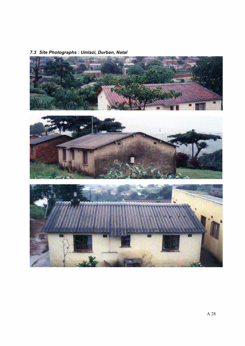
A 28

7.3 Site Photographs : Umlazi, Durban, Natal

A 29

7.4 Socio-demographic summary: Umlazi 1 TOWNSHIP DETAILS: Township Number 39 Stands percentage 95% Number of homes 780 Average rainfall 1016mm Minimum temperature 11 C Tarred roads All Distance to nearest city 35km 2 DATABASE DETAILS:

Loggers uploaded 13 Total readings taken 1745141 Size 49 MB 3 GROUP STATISTICS: 3.1 Per Household criteria Mean Median Std. dev Min Max Household size [people] 5.857 5 9.216 1 15 Monthly income [R] 1869 1400 1621 200 8000 Highest education rating 11.56 12 1.621 6 13 3.1.1 General Ownership of dwelling 100% Small business presence 3.18% 3.1.2 Appliance ownership Stove with oven (3 plate) 7.94% Stove with oven (4 plate) 50.79% Hotplate 39.68% Heater 30.16% Kettle 61.90% Iron 82.54% Geyser 9.52% Washing machine 3.18% Television 77.78% Lights 96.83% Fridge/fridge-freezer 79.37% Freestanding deep freeze 25.40%

A 30


3.2.2 Roof materials: IBR/Corrugated Iron/Zinc 42.86% Thatch/Grass 0% Wood/Masonite/Board 0% Brick 1.59% Blocks 0% Plaster 0% Concrete 0% Tiles 4.76% Plastic 0% Asbestos 50.79% Daub/Mud/Clay 0% Outstanding roof materials 0% 3.2.3 Wall materials: IBR/Corrugated Iron/Zinc 0% Thatch/Grass 0% Wood/Masonite/Board 0% Brick 96.83% Blocks 1.59% Plaster 0% Concrete 0% Tiles 0% Plastic 0% Asbestos 1.59% Daub/Mud/Clay 0% Outstanding Wall materials 0% 3.2.4 Water service: Piped water in the house 57.14% Tap in yard 42.86% Communal tap 0% Water sources outstanding 0%

A 31

4 ALTERNATIVE FUEL SOURCES: 4.1 Local price of alternative fuels: Electricity R0.2933 /kWh Coal R Paraffin R 2.50 Gas R 2.14 Wood R 2.12 4.2 Reported use of alternative fuels: Coal 0% Paraffin 26.98% Gas 1.59% Wood 0% Charcoal 0% 5 ELECTRICITY SUPPLY: 5.1 Supply capacity: Mean Median Std. dev Min Max Main switch size [A] 58.1 60 10.69 60 60 Years electrified 7.127 7 4.77 1 16 5.2 Quality of supply - complaints: Power failure 19.05% Lights get dim at night 1.59% Main switch trips 11.11%

A 32

8. Walmer Dunes, Port Elizabeth, Eastern Cape

8.1 Site synopsis: Walmer Dunes This site features 50% electrification, in an area where only arterial roads are tarred. The area is 7km from a city centre. Inhabitants are 20 % poorer than the national average. Water is obtained from a tap in the yard, and most houses are completely built from corrugated iron. About 50% of households have a TV. The climate is moderate here, and alternative fuels are not used much. 40% report using paraffin. Consumers are happy with their QOS.

8.2 Load data: Walmer Dunes Table 13: Logging information: Walmer dunes Item Data Start: 13/5/97 Finish: 4/9/97 Channels: 80 Data points: 2,308,758 Logging efficiency: 0.89 Size of database (MB): 68.71 Table 14: Peak load data: Walmer dunes Peak no. Date Itot [A] N I ave[A] Std Dev [A]

1 29/6/97 19:40 200.2 71 2.82 3.83 2 25/7/97 19:30 200 71 2.82 3.74 3 18/7/97 19:05 198.7 71 2.80 4.91 4 2/6/97 19:25 198.6 71 2.80 3.44 5 13/6/97 18:55 193.3 71 2.72 4.25

A 33

8.3 Site Photographs: Walmer Dunes, Port Elizabeth, E. Cape

A 34

8.4 Sociodemographic summary: Walmer Dunes 1 TOWNSHIP DETAILS: Township Number 41 Stands percentage 50% Number of homes 6000 Average rainfall 611mm Minimum temperature 0 C Tarred roads Main only Distance to nearest city 7km 2 DATABASE DETAILS:

Loggers uploaded 12 Total readings taken 2308758 Size 69 MB 3 GROUP STATISTICS: 3.1 Per Household criteria Mean Median Std. dev Min Max Household size [people] 3.712 4 4.517 1 10 Monthly income [R] 854.2 700 969.6 200 8000 Highest education rating 9.781 10 2.235 3 13 3.1.1 General Ownership of dwelling 100% Small business presence 0% 3.1.2 Appliance ownership Stove with oven (3 plate) 6.85% Stove with oven (4 plate) 10.96% Hotplate 47.95% Heater 12.33% Kettle 64.38% Iron 76.71% Geyser 0% Washing machine 2.74% Television 64.38% Lights 100% Fridge/fridge-freezer 30.14% Freestanding deep freeze 4.11%

A 35


3.2.2 Roof materials: IBR/Corrugated Iron/Zinc 98.63% Thatch/Grass 0% Wood/Masonite/Board 0% Brick 0% Blocks 0% Plaster 0% Concrete 0% Tiles 0% Plastic 0% Asbestos 1.37% Daub/Mud/Clay 0% Outstanding roof materials 0% 3.2.3 Wall materials: IBR/Corrugated Iron/Zinc 84.93% Thatch/Grass 0% Wood/Masonite/Board 6.85% Brick 1.37% Blocks 5.48% Plaster 0% Concrete 1.37% Tiles 0% Plastic 0% Asbestos 0% Daub/Mud/Clay 0% Outstanding Wall materials 0% 3.2.4 Water service: Piped water in the house 0% Tap in yard 100% Communal tap 0% Water sources outstanding 0%

A 36

4 ALTERNATIVE FUEL SOURCES: 4.1 Local price of alternative fuels: Electricity R0.2225 /kWh Coal R 0.72 Paraffin R 2.60 Gas R 6.60 Wood R 0 4.2 Reported use of alternative fuels: Coal 0% Paraffin 38.36% Gas 4.11% Wood 0% Charcoal 0% 5 ELECTRICITY SUPPLY: 5.1 Supply capacity: Mean Median Std. dev Min Max Main switch size [A] 60 60 0 60 60 Years electrified 3.055 3 0.5708 1 4 5.2 Quality of supply - complaints: Power failure 0% Lights get dim at night 0% Main switch trips 2.74%

APPENDIX B:

NRS Load data collection guide

THE NRS LR PROJECT:

LOAD DATA COLLECTION

GUIDE

By Dr R Herman (University of Stellenbosch)

M Dekenah (Marcus Dekenah Consulting cc) October 1997 (2nd Revision)

Appendix B: Contents `1. INTRODUCTION

2. WHO WILL COORDINATE THE PROJECTS?

3. WHY LOAD DATA IS COLLECTED

3.1 LOAD DATA FOR ELECTRICAL RETICULATION DESIGN 3.2 LOAD DATA FOR FORMULATING TARIFFS 3.3 LOAD DATA FOR DEMAND SIDE MANAGEMENT

4. WHERE SHOULD THE INFORMATION BE COLLECTED?

4.1 COMMUNITY STABILITY 4.2 EXTENT OF ELECTRIFICATION 4.3 LEVEL OF CONSUMPTION 4.4 COMMUNITY CO-OPERATION

5. GETTING STARTED

5.1 METHOD OF LOGGING: SAMPLE SELECTION 5.2 SIZE OF PROJECT: NUMBER OF CONSUMERS MONITORED 5.3 HOW TO SELECT THE LOGGING SITES 5.4 BUDGETING CONSIDERATIONS

5.4.1 Funding 5.4.2 Project timing 5.4.3 Selection & Training of staff

5.5 INSTALLATION OF HARDWARE, DOCUMENTATION & INITIALISATION 5.5.1 Installation

5.5.1.1 Installation of a logger up a pole 5.5.1.2 Installation of logger inside street furniture

5.5.2 General installation tips 5.5.2.1 Connection of current “channels” 5.5.2.2 Plug-orientation 5.5.2.3 Further installation tips

5.5.3 Documentation of the site 5.5.4 Initialisation of loggers

5.5.4.1 Initialisation values 5.5.4.2 Data transfer cables 5.5.4.3 What to do if a logger refuses to communicate

5.5.5 First download of data

6. COLLECTION, QUALITY CONTROL & PROCESSING OF DATA

6.1 ALLOCATION OF FILE NAMES TO DATA 6.2 QUALITY CONTROL OF DATA 6.3 TRANSMISSION OF DATA TO PROJECT MANAGER

6.3.1 Transmission by post 6.3.2 Transmission of data by E-mail

7. COLLECTING SOCIO-DEMOGRAPHIC INFORMATION FROM CONSUMERS

7.1 PREPARATION PHASE 7.1.1 Community contacts 7.1.2 Selection & Training

7.1.2.1 Selection 7.1.2.2 Training of interviewers

7.2 EXECUTION OF SURVEYS 7.3 EVALUATION OF RESULTS & BACK-CHECKING 7.4 SECURITY OF PERSONNEL

8. FEEDBACK

9. NRS LOAD RESEARCH PROJECT: CONTACT LIST

10. TERMINOLOGY

10.1 LOAD DATA. 10.2 DATA LOGGERS. 10.3 LOAD SAMPLES. 10.4 COINCIDENT LOGGING. 10.5 SAMPLE SIZE. 10.6 SAMPLING INTERVAL. 10.7 AVERAGING INTERVAL. 10.8 HOST COMPUTER. 10.9 DOWN-LOADING DATA.

11. ADDENDUM A: LOGGER DOCUMENTATION SHEET

12. ADDENDUM B: LOGGER INITIALISATION PROCEDURE

13. ADDENDUM C: LOGGER DOWNLOAD PROCEDURE

1 INTRODUCTION The NRS LR project is a co-ordinated effort amongst Municipalities, Universities, and ESKOM to get collect data about low-income domestic consumers in order to design electricity supply networks for them which are both reliable and cost effective. Two types of data are collected:

1. Load data, from multi-channel electronic data-loggers attached to the consumers house-connection

2. Socio-demographic data, about the consumers living in those houses. This data is collated and analysed together with climate data, by the project manager, who then feeds the data back to the NRS, and the various projects. This allows the latest design data to be made available to organisations busy with electrification. This brief guide is intended to give some assistance to all those participating in the NRS 034 National Load Research Programme - let's call it LR for short. In this guide you will find information on ● Why, where, and how load data must be collected ● How the data is to be collated, quality controlled and processed

● How the information will be made available to those taking part in the programme. A list of contacts is included at the end of this document. If you have any queries, please do not hesitate to contact either the project manager, or one of the project specialists.

2 WHO WILL COORDINATE THE PROJECTS? It is important for the LR project to be coordinated for maximum benefit. If all the load data are collected in the same way, it will make it easier to compare classes. This requires some standardisation in both the hardware and software of the data loggers. The demographic parameters of each load class must also be collected in a unified manner. A dependable data-base must be constantly maintained at a central point. For this reason, a project manager is coordinating this project. See the “who to call” section at the end of this document for important contact information.

3 WHY LOAD DATA IS COLLECTED Some of you may not be convinced such an exercise is necessary. Here are a few reasons why the collection of residential electrical load data is important to the electricity supply industry. 3.1 LOAD DATA FOR ELECTRICAL RETICULATION DESIGN You are probably aware of the national drive to provide electricity to the large portion of our population who do not have this facility. The basic need here is to drive costs down, whilst still meeting the needs of the consumer. These systems can only be economically designed if adequate knowledge of the anticipated loads is known. In the past consumer load parameters have been a matter of guess-work. If we want exacting designs we need good load data on which to base our load estimates. There are three particular areas in reticulation design that require statistical description of the electrical loads. They are: ● Calculation of voltage drops in feeders ● Thermal sizing of feeders and transformers

● Calculation of transmission losses Voltage drop algorithms have been researched (by the NRS 034 Voltage Drop Task Force) and methods have been identified that use statistical models of the load currents. These methods are superior to the existing deterministic (i.e. non-statistical) methods. However, these statistical methods can only be used if the statistics of the design load parameters are known. And the statistics, in turn, rely on the collection of load data from a variety of representative areas. Research is continuing to find ways of using these load statistics for thermal sizing of conductors (particularly ABC's). A project is also underway to apply the knowledge of annual load shapes to the calculation of feeder losses. 3.2 LOAD DATA FOR FORMULATING TARIFFS Tariffs are also receiving more attention in recent times. Time-of-use tariffs are either being applied in some areas or are under consideration. Suppliers of electricity must know what the load patterns look like when designing tariffs. These data can be supplied from an extensive LR project. 3.3 LOAD DATA FOR DEMAND SIDE MANAGEMENT Although still in its infancy, demand side management, (DSM), i.e. the influence of load behaviour through external means, is becoming important. Strategies are being formulated by which load patterns can be manipulated to the advantage of the supplier and, ultimately, the consumer. On-going load surveys will give much-needed input into the solution of the related DSM problems.

4 WHERE SHOULD THE INFORMATION BE COLLECTED? The greatest need at the moment is for load information about the lower income groups. The focus right now is on low-income, informal and rural consumers, who have an average

consumption of less than 250 kWh/month, and who have been electrified for about two years or more. These load classes should therefore receive priority. The project may later be expanded to include all the consumer classes. An emerging “middle class” of consumer is perceived to become important in the future. There are a few issues which require consideration when targeting a community for a load survey. They are mentioned briefly below. The community should be stable, moderately electrified and be co-operative to the project. 4.1 COMMUNITY STABILITY By this we mean the way the community has responded to the supply of electricity. One should establish whether consumers have a record of paying for their supply. Confirmation of this may be obtained from the utility supplying the electrical power. The other question which requires an answer is whether there are illegal connections and the extent of the problem. There are several reasons for extracting this information. A community that has a bad record of payment could view the monitoring of loads in its area with some hostility. There would then be the danger of equipment damage. Demographic data collected from this type of community would also be unreliable because of suspicion from the consumers. 4.2 EXTENT OF ELECTRIFICATION The target community should have a high degree of electrification. There should not be many gaps in connectivity. First-time consumers require a period of adjustment to the use of electrical power. Individual load patterns would be expected to be somewhat erratic for the first two years. So, even if the community is identified as "newly electrified", it should have been operative for at least 24 months before a load survey is done. 4.3 LEVEL OF CONSUMPTION Since we are initially looking for load models for the lower income groups, the target community should have an average consumption of less than 250 kWh per metered point. This can be established by taking the reading on a check meter and dividing by the number of connected households. Alternatively, if there is no check meter, monthly billing data can be used for this purpose. 4.4 COMMUNITY CO-OPERATION This is a very important facet of the load survey. Local leadership (civics and/or local authorities, or any other area leadership) should be approached before commencing with load data acquisition. The purpose of the load survey should be explained to these bodies.

5 GETTING STARTED The process of starting on of these projects is the following: ● Identify a community, method of logging and number of data-loggers required ● Obtain funding

● Secure equipment ● Secure manpower ● Install the hardware, initialise it and document the site

● Down-load data regularly (i.e. monthly) Refer to the previous section for section of the community. 5.1 METHOD OF LOGGING: SAMPLE SELECTION Having decided on the community to be monitored, attention must be given to the selection of sites for installation of the data loggers. 5.2 SIZE OF PROJECT: NUMBER OF CONSUMERS MONITORED Try to monitor a minimum of 70 , but preferably 100 consumers (Error in sampling gets better as the number of samples increase. This number has been chosen for statistical significance). The number of data loggers required to conduct a statistically significant load survey will depend on the number of channels on the logger. It will also depend on whether it is possible to employ all the channels at each site. If, for instance, only 4 consumers can be monitored from each pole-mounted installation in a given community, then 25 loggers will be required for a sample size of 100. 5.3 HOW TO SELECT THE LOGGING SITES It is recommended that a random systematic method be used. This is explained below:

1. List all the dwelling stand numbers from the township plans. 2. Divide the number of stands by the number of available loggers (call the resulting

number Sl, say.) 3. Select a random starting point, say at stand Sp. 4. Add multiples of Sl to Sp to give the stand numbers at which to site the loggers.

5. Check (4) to ensure that all or most of the data channels can be used at the point under consideration.. If necessary move to one pole forward or backward.

The above process is repeated until all the loggers have been sited. Meticulous attention must now be given to identifying each monitored dwelling with its logger and channel. See the section on project documentation.. At this stage you will have a good idea of how many loggers will be required to run the project. Add 10% as a reserve, in case of problems or theft, and secure the funding.

5.4 BUDGETING CONSIDERATIONS It is necessary to have the right equipment and manpower for a sustainable load research project. 5.4.1 FUNDING Nothing happens without money. A preliminary budget for a project would look like the following: ITEM COST(R)

Data loggers for 80+ consumers (depends on connection efficiency)

32 000 - 47 000

Lap-top computer & software '486 or better, with car-charger.

5 000 - 10 000

TOTAL CAPITAL COST (once per project)

37 000 - 57 000

Include maintenance budget (per year, downloading at 1-2 days per month, excluding any analysis)

96 - 192 hours

Since embarking on this project will inevitably lead to lower capital costs, (over-design may be in the order of 500%), as well as provide better knowledge of the consumer, his quality of supply, and his perception of the above, the cost is justifiable. Type of logger Loggers should be able to record voltage and current traces and store these values in memory, for downloading to a personal lap-top computer. Please check with the project manager to see if your type of logger can be accommodated. Data loggers which can average over 5 minute intervals have been selected. Our current supplier of preference is ESKOM (TRI 5001). We have found this locally developed product to be suitable and affordable. The price of these data loggers is in the region of R 2 350 per unit (500 KB RAM), including software, cable, and manual. (See contacts at end of document)

5.4.2 PROJECT TIMING Experience has shown that the fastest time possible to get one of these projects under-way is about 3 months: ● Delivery time on data-loggers is about 6 weeks ● Staff must to be seconded and trained ● Loggers have to be installed ● The project must be documented ● Start-up problems have to be solved ● A system for quality control of data must be established ● Management-control systems must be established

The amount of time necessary to accomplish this must not be under-estimated ! 5.4.3 SELECTION & TRAINING OF STAFF A particular type of person is needed to run this type of project. This person must be : ● Computer literate ● Meticulous (system oriented & organised) ● Motivated & interested. The selection of the right type of person is important because a huge mass of data are generated by this type of project, and a little disorganisation can very quickly lead to chaos. Staff who are directly involved in the project attend the workshop which is held in November each year, where training is given. The cost of the workshop is nominal. Please contact the project manager for details.

5.5 INSTALLATION OF HARDWARE, DOCUMENTATION & INITIALISATION Metering hardware must be installed and initialised correctly, which normally involves the following steps: ● Install the meters ● Document connection (see Addendum A) ● Initialise the logger (see Addendum B)

● Carry out first download one week later (see Addendum C) There are sometimes “starting pains” associated with a logging programme. The following steps must be followed quickly to avoid typical start-up problems. 5.5.1 INSTALLATION There are several types of logger. Please read the instruction manual to see what it can tolerate environmentally. As a general rule, avoid any arrangements that allow the logger to be exposed to moisture, heat, insects, vandalism & theft.

There are only two options for mounting of loggers: ● Inside street furniture

● Up a pole While the installation of loggers is not permanent, it should be good enough to last safely for a period of 2 years.

5.5.1.1 Installation of a logger up a pole The logger must be housed inside a waterproof box out of reach, a reasonable height above the ground. There are a number of things to watch out for: ● Ensure the pole-box is large enough to accommodate the logger safely, and that the

action of closing the cover of the box does not interfere with the power & instrumentation leads.

● The box is normally out of reach. This makes downloading difficult unless a long data

cable is made up, strapped permanently onto the pole, and terminated at head-height in a small pratley box, strapped to the pole. This arrangement means the person doing downloading need not carry a ladder to access the data logger.

● The box must be weather-proofed. Pole-enclosures for the loggers need not be expensive. Opaque 5 litre plastic milk bottles, (inverted and strapped to the pole) have proved very successful.

5.5.1.2 Installation of logger inside street furniture Usually, underground low voltage distribution systems are distributed from a pavement-mounted distribution kiosk. These are generally fitted out with consumer circuit-breakers and kWh meters. There are a number of things to watch out for: ● The data logger should be placed in a position where it will not be affected by dampness

from the ground. ● Insects can be a problem here so make use of insecticide spray where necessary. ● Mount the logger firmly (using cable ties). Kiosks are regularly accessed by other

personnel, so a free logger resting on a flat surface is easily dislodged or tampered. ● Door-seals on street-furniture are not water-proof, particularly in areas which experience

wind & rain at the same time. Loggers need to be mounted in a position where they are out of spray. Water-logged data loggers are a potential earth-leakage hazard.

5.5.2 GENERAL INSTALLATION TIPS

5.5.2.1 Connection of current “channels” Fill all instrumentation channels linearly (i.e. from 1 upwards) to the maximum number of consumers available at that metering point. Do not leave any gaps. This will use up data logger memory more efficiently.

5.5.2.2 Plug-orientation Be aware that plug orientation is important for some loggers (i.e. which plug in which socket). Labels on the instruments are generally clear with respect to connector details and indicate which is the voltage input. Make sure that connections are done correctly, otherwise it could lead to internal hardware damage!

5.5.2.3 Further installation tips ● Remember that the CT’s used may be of the “wedding ring” type and connection of

the CT will require the conductor to be disconnected from the supply and fed through the centre of the CT. This will require the skill and qualification of a licensed wireman as an electric shock can occur while disconnecting the supply wire.

● Make sure that connections are made properly and that screw-terminals are tight. ● When conductor insulation material is stripped away for connection purposes, make

sure that the screw terminal makes contact with the conductor. ● If the logger is housed in a box with a lid, be careful not to dislodge the plugs &

wiring when closing the lid after a download. Similarly, do not allow a logger to hang by its instrument leads.

5.5.3 DOCUMENTATION OF THE SITE During the installation of the loggers, it is imperative that the sheet in Addendum A is completed METICULOUSLY, for each logger, and kept in a safe place: These tables are essential for record-keeping, and will be referred to repeatedly during the project. Check them to ensure they are right the first time! Forward a copy of these documents to the project manager immediately after installation. 5.5.4 INITIALISATION OF LOGGERS Read the data logger manual, and practice with the software before going on-site. A lap-top computer, data-cable and communication software are required. Loggers must be initialised: ● The first time installed at a pole/kiosk. ● If moved/swapped to another pole/kiosk

● After return from repairs.

5.5.4.1 Initialisation values Set the logger up, (once installed), to the following settings: ● Reading averaging time = 300 seconds (5 minutes) ● Clock on the logger synchronised to the PC clock (which has the correct time). ● Logger identity code (ID) set to a unique two-digit number (see data-handling later) . ● Logger set up to monitor the number of channels which are connected. Write the logger ID onto the outside of the logger. This will help with the downloading procedure.

5.5.4.2 Data transfer cables Data-cables are not standard things. A lap-link-cable may not work. If extension cables are made, ensure they are pin-copies of the original. Read the manual.

5.5.4.3 What to do if a logger refuses to communicate If the logger is either dead, or has a communications problem then: ● Check the data-cable (try another logger). ● Check the communications port on the computer. ● Check the fuse inside the logger (if any). ● Read the manual.

Send it back to the supplier immediately for repair if none of the above work! 5.5.5 FIRST DOWNLOAD OF DATA Within 10 days of first installation, all loggers should be downloaded. The downloading software, is not intuitive, use the downloading procedure of Addendum C

at the end of this document to avoid problems. It is recommended that a copy is taken into the field and followed exactly. Practice with the software and a logger before going into the field.

The data should be checked for the following problems: -Data logger clock & time set correctly -Internal logger ID-code set correctly -Correct number of data channels enabled -Data being logged -Confirm the logger is reading the correct currents and voltages! Thereafter, data loggers should be downloaded monthly.

6 COLLECTION, QUALITY CONTROL & PROCESSING OF DATA The downloading process normally involves going to each logger, with a lap-top computer, connecting a communications cable to it, and getting it to pass the stored data to the PC. During this process, the operator must furnish a file-name, manage a large amount of files, and carry out quality control of the data to see each logger is operating OK. 6.1 ALLOCATION OF FILE NAMES TO DATA Since a large amount of data is being centralised on the NRS LR database, a system must be used to ensure that: ● No two townships can supply different files with the same name ● File origin & age is easily recognised by the filename

● Large quantities of files are manageable Use this system for naming of files when downloading: “Lxx_mmdd.zzz” Where: L = letter standing for the nearest major city. (W=Witbank, J= Johannesburg etc.) xx = unique logger ID code (marked on outside of logger). _ = underscore (or placeholder if more than 100 loggers). mm = month of the year(ie June = 06). dd = day of the month(ie 17th =17). zzz= file extension automatically given to file by software. Note that the file-naming convention only allows 8 characters for the “name” part. Example: Downloading logger 03 near Johannesburg on 17th June will give J03_0617. This system has been chosen because it allows files to list logically in a Windows file-manager/explorer. It also has only eight characters, so that management by windows 3.x software is still possible. If some files get “mixed” refer to the Logger ID in data-file header. Since this value is automatically assigned by logger, from the initial set-up. 6.2 QUALITY CONTROL OF DATA Although the data files collected from the data loggers may be in *.xls format, they are not exactly MS EXCEL. The format of the original files will be corrupted if they are re-saved under MS EXCEL. Avoid tampering with the original data files at all costs! Special software has been developed to look at the data-files from the data loggers. This software has been developed specifically to help with quality control of data, and will very quickly allow faulty loggers, power failures etc. to be pin-pointed. Request your free copy of “Dataview” from the project manager. The software is also useful for QOS & consumption surveys.

Use Dataview to scan each file which is downloaded and to look for any abnormalities. As each file is scanned , draw its start and finish dates onto a chart, for each logger ID. This will reveal the following problems immediately: ● A logger not down-loaded (it easily happens) . ● Logger memory not cleared after a download. ● Internal date/time clock of the logger has not been set correctly ● Logger ID missing or has been duplicated.

● Logger malfunctioning (i.e. no data). 6.3 TRANSMISSION OF DATA TO PROJECT MANAGER The collected data must be sent to the project manager as soon as it has been retrieved from the field. Electronic mail is preferred, however the postal service is also acceptable. “Zip” all of the files from a single download onto a “stiffy” disk/s. Keep a copy, and send one to the project manager via post or E-mail. 6.3.1 TRANSMISSION BY POST Please ensure that stiffies are wrapped in “bubble” plastic. Post does not always arrive. Please check this with the project manager. Please note on the data : ● Where it is from ● When it was downloaded

6.3.2 TRANSMISSION OF DATA BY E-MAIL There are several E-mail packages available, and they are not fully compatible and can react differently when transferring large amounts of data. The secret is to find the right recipe and write it down for later reference. Do not change the recipe. Here are some general hints: ● “Attach” data-files in preference to “enclosing” them.

● If operating Group-wise or MS-mail, expect a problem related to file-size. Files sometimes have to be zipped into a number of smaller chunks.

7 COLLECTING SOCIO-DEMOGRAPHIC INFORMATION FROM CONSUMERS Socio-demographic data about the logged consumers is essential for the LR project. It is being used to relate such parameters as the type of house construction, the climate, family size etc. of the township to the measured electrical loading. The individual consumers who are being logged must supply this information. A special questionnaire has been prepared for this purpose. Please check with the project manager to see that you have the latest version of the questionnaires. This section covers advice on how to handle the surveys: ● What preparations must be undertaken. ● How to execute surveys. ● Evaluation and checking of the results.

It is strongly recommended that a professional market-research contractor is used to carry out the surveys. This will save a considerable amount of (start-up and running) time and increase the quality of results. The personnel are generally well-trained, and only need to be briefed. Please check with the project manager to see whether this work will be carried out by a Market Researcher appointed with NRS LR funding. 7.1 PREPARATION PHASE During this phase the whole “exercise” must be lined up. Community contact must be made and interviewers must be selected and trained. 7.1.1 COMMUNITY CONTACTS If there are community channels, use them to ensure that the survey is supported. Try not to ask for permission to carry out the survey. This may take a long time to obtain. 7.1.2 SELECTION & TRAINING Preparation is crucial to quality of results.

7.1.2.1 Selection The surveyors should be picked specifically to fit in to the local environment. They should be of the same colour and language group as the sample population. Surveyors should be literate, meticulous, and outgoing. Choose enough surveyors to work through the community in a day, because foreknowledge in the community can distort results. About fifteen surveyors should be acceptable.

7.1.2.2 Training of interviewers Plan a training session amongst the surveyors for a couple of days before. Interviewers must be briefed extremely well so that they know exactly why the interviews need to be done and what each question means. This will enable them to explain the questions if necessary. Role-playing is an effective method of training, since it gives each surveyor a chance to practice and to be on the receiving end. Surveyors who cannot role-play successfully should not be used on the community. Completeness of information is important for this questionnaire, and surveyor's should be briefed as to what actions to take in case of refusals, don’t-knows and no-one-homes. 7.2 EXECUTION OF SURVEYS During the execution , the supervisor should equip each surveyor with his call list, giving sites to survey. He should manage the process to be finished within a day. 7.3 EVALUATION OF RESULTS & BACK-CHECKING Have all forms checked visually by one or two people. There are certain places in the “people” side of the form where the reported number of people in each question-table should be the same. See that they are. 7.4 SECURITY OF PERSONNEL In poorer areas, it is not uncommon for interviewers to be assaulted or robbed. Take a first-aid kit. Staff should be wary of highjackings.

8 FEEDBACK A feedback session will be arranged ( probably in November) each year. At this session the various participants will be able to share their experiences. A report will be issued soon after this. This should be available early in the next year.

9 NRS LOAD RESEARCH PROJECT: CONTACT LIST WHO TO CONTACT FOR HELP OR INFORMATION During the course of the data collection programme you may want to ask questions. In order to satisfy this need we have set up a contact list. Please do not hesitate to contact the project manager if you have any problems.

Role Contact person Telephone Fax E-mail Project administration, File handling,

Data-base work,

Latest analysis

Mr. Marcus Dekenah

25 Maluti Ave

Doringkloof 0157

012-667-1347 083 3061771

012-667-1347 [email protected]

Project consultant

(General)

Mr C T Gaunt 021-4699100 021 245571 [email protected]

Project consultant (Statistics)

Prof JS Maritz 021-9380357 021 9380310 [email protected]

Project consultant

(Research)

Dr R Herman 021-808-4323 021-808-4981 [email protected]

Source: ESKOM data loggers

Mr Pierre Doman 011-629-5005 011-629-5366 --

Load researcher:

Walmer dunes project

Mr J Westraadt 041-3924139 041343789 --

Load researcher:

Sweetwaters project

Mr D Baker 0331-456211 0331-428802 [email protected]

Load researcher:

Mont-Clare project

Mr D Greyling 011-4907471 0114907590 [email protected]

Load researcher:

Umgaga & Umlazi

Mr V Nagessar 031-3001185 031 3001010 [email protected]

10 TERMINOLOGY It will be an advantage if common terminology is used when referring to various aspects of load data collection. Here are a few definitions:- 10.1 LOAD DATA. This refers to the collected electrical load currents drawn by residential consumers, recorded at regular intervals. 10.2 DATA LOGGERS. These are stand alone devices which can be programmed to sample load currents at regular intervals. 10.3 LOAD SAMPLES. These are the individual load currents stored by the data loggers. 10.4 COINCIDENT LOGGING. All the loggers within a group survey should be synchronised with one another so that the loads are all sampled at the same time. This is known as coincident logging. 10.5 SAMPLE SIZE. Sample size refers to the number of consumers monitored in a given area. 10.6 SAMPLING INTERVAL. Load currents are sampled on a continuous basis by the data loggers at a rate determined by the logger design. This interval is small (about 0,5 seconds). 10.7 AVERAGING INTERVAL. The sampled load currents are averaged over an averaging interval and these averaged values are stored in the memory of the data logger. This averaging interval may be set by the operator (usually from 0,5 minutes to an hour or longer). 10.8 HOST COMPUTER. Data are transferred from the memory of a logger to a host computer. This is usually a portable lap-top or "note-book" type of PC which uses a program especially coded for communicating with the logger. Dedicated software is required to perform this operation and will be supplied by the manufacturers of the data loggers. The host computer must have a "real-time-clock" which is set correctly before each data retrieval session. The host computer can also mean a table-top PC which is used for the same purpose but the loggers are then swapped on site and taken to the host computer for data retrieval. This may only be done if the data logger has a non-volatile memory.

10.9 DOWN-LOADING DATA. This is the process that transfers the recorded load data from a logger to the host computer.

11 ADDENDUM A: LOGGER DOCUMENTATION SHEET This serves as a permanent reference of where a logger is connected, and what consumers it is connected to. Fill in one of these per logger. It is essential that all of this information is 100% correct, as it will be used: ● To guide market research to the right house. ● To set-up loggers when they return from repairs.

● For analysis by NRS of load against market research data for each house.

Logger ID:

Date Installed:

S/S no. Feeder no. Pole/kiosk no. Channel no. Erf Address Comments: 1

2

3

4

5

6

7

12 ADDENDUM B: LOGGER INITIALISATION PROCEDURE Procedure is described for the TRI 5001 logger as at 97/9/15. (Only to be performed on installation/replacement of a logger) Before leaving for site, ensure that the time-clock on the lap-top is correctly set to local time signal. The following equipment is required: ● Lap-top & spare battery or car-charger. ● Data cable.

● Data-logger documentation (Addendum A). PROCEDURE

1. Before any equipment is connected, check to see if the logger light is flashing. If not, it may indicate a fault.

2. Plug in data-cable (proprietary for data logger). 3. Type ‘LOGGER1’ [ Enter ]. The communication software should start. 4. Push [ F2 ]. The set-up menu should display. 5. Set the logger ID & no. of channels exactly according to this logger-sheet (see

Addendum A). 6. Push [ 7 ] to clear the data memory, [ Y ] to confirm. 7. Push [ F4 ] to synchronise the logger to the lap-top’s date & time. 8. Select “Monitor”, and verify the real time readings from the logger are OK. 9. Push [ 8 ] to exit & resume logging. The light on the logger should start to flash a short

while after the cable is disconnected. The logger is collecting data. 10. Push [ Alt +X ] to exit the communication software.

11.

13 ADDENDUM C: LOGGER DOWNLOAD PROCEDURE Procedure for TRI 5001 7-channel logger as at 1997/9/15 Before leaving for site, ensure that the time-clock on the lap-top is correctly set to local time signal. The following equipment is required: ● Lap-top & spare battery or car-charger. ● Data cable.

● List of data-loggers, their positions & ID’s PROCEDURE

1. Before any equipment is connected, check to see if the logger light is flashing. If not, it may indicate a fault.

2. Plug in data-cable (proprietary for data logger). 3. Type ‘LOGGER1’ [ Enter ]. The comms software should start. 4. Push [ F2 ]. The set-up menu should display. 5. Push [ F3 ] to download data. Enter the filename [ Enter ] .The file will transfer to the

lap-top. 6. Push [ 7 ] to delete the data memory, [ Y ] to confirm. 7. Push [ F4 ] to synchronise the logger to the lap-top’s date & time. 8. Push [ 8 ] to exit & resume logging. The light on the logger should start to flash a short

while after the cable is disconnected. The logger is once again collecting data. 9. Push [ Alt +X ] to exit the comms software.

Date post:	04-Jan-2022
Category:	Documents
Upload:	others
View:	3 times
Download:	0 times

THE NRS NATIONAL LOAD RESEARCH PROJECT: 1997

Documents