The Optimal Length of Contracts

with Application to Outsourcing

Matthew Ellman∗

Universitat Pompeu Fabra

February, 2006

Abstract

This paper resolves three empirical puzzles in outsourcing by formalizing the adaptation

cost of long-term performance contracts. Side-trading with a new partner alongside a long-

term contract (to exploit an adaptation-requiring investment) is usually less effective than

switching to the new partner when the contract expires. So long-term contracts that prevent

holdup of speciÞc investments may induce holdup of adaptation investments. Contract

length therefore trades off speciÞc and adaptation investments. Length should increase

with the importance and speciÞcity of self-investments, and decrease with the importance

of adaptation investments for which side-trading is ineffective. My general model also shows

how optimal length falls with cross-investments and wasteful investments.

Jel Classification numbers: D23.

Keywords: Contract length; market forces; incomplete contracts; holdup.

∗I thank Erik Beulen, Ramon Campabadal, Oliver Hart, Ashok Kaul, Eric Maskin, Elisenda Monforte,

Michael Raith, Jan Sarsanedas, Andrei Shleifer, Jer�ome Vandenbussche, Abe Wickelgren and seminar partic-

ipants at ASSA (2005), the Toulouse IDEI Conference in Honor of Jean-Jacques Laffont (2005), the Harvard

Kennedy School, the Kellogg School of Management, and Autonoma de Barcelona, Northwestern, Tilburg, Tor-

cuato di Tella Universities for helpful comments. I gratefully acknowledge Þnancial support from the European

Commission (HPMF-CT-1999-00317), the Spanish Ministry of Science and Technology (BEC 2003-00412) and

CREA (Barcelona Economics). Comments gratefully received at Matthew.Ellman@upf.edu.

1

1 Introduction

Transactions Cost and Incomplete Contract theorists have shown how long-term contracts

help protect relationship-speciÞc investments (see Williamson, 1975 and 1985, Klein, Crawford

and Alchian, 1978, and the formalization in Grout, 1984), but we know little about the costs

of extending contract length. This paper formalizes a simple yet powerful idea: long-term

contracts may obstruct beneÞcial market forces. My conceptual contribution is to show how

and when this market-shielding cost arises. I also formalize two other major costs of contract

duration. I then represent the costs and beneÞts of contract duration within a single theoretical

model in order to derive optimal contract length. Using the market-shielding results alone, the

paper is able to resolve three signiÞcant puzzles from the empirical literature. My framework

also throws light on the practical challenge of designing ßexible long-term contracts.

Contracts vary greatly in length. Multi-year contracts are common in, for example, con-

struction, contract manufacturing, distribution, franchising and Information Technology (IT).

Outsourcing in IT presents an instructive showcase.1 For instance, IBM Global Services sells

IT services to Nokia, Hertz, American Express (Amex) and Deutsche-Bank (DB) under 5, 6,

7 and 10 year contracts, respectively. I will use IBM�s $4bn deal with Amex (see Weiss, 2002)

to illustrate the main ideas of the paper. Signed in February of 2002, the contract essentially

obliges IBM to manage and maintain Amex�s Information System (IS) at a predetermined

price. I call this exchange the �basic trade.�2 The contract duration is 7 years - it enforces the

basic trade from 2002 till 2009 - but through renegotiation and renewal, Amex could have paid

IBM to provide the same services under a sequence of longer or shorter contracts. I therefore

ask: what are the costs and beneÞts of increasing contract length?

I begin with an example of the now familiar beneÞts. IBM invested in organization and

planning to lower its costs of managing Amex�s Information System. Many of these invest-

ments are partly speciÞc to Amex. For instance, IBM coached 2000 workers who transferred

from Amex to IBM in 2002. This reduced IBM�s cost of servicing Amex, but the transferred

workers� speciÞc knowledge of Amex does not help IBM in servicing other clients. So IBM

must sell services to Amex if it is to fully exploit its cost-reducing investment. Under short-

term contracting, Amex could therefore extract a share of the cost-reduction by refusing to

buy unless IBM lowers its price. This �holdup� by Amex reduces IBM�s investment returns,

1The IT outsourcing market was worth over $569bn in 2003, up 6.2% from 2002 (Pruitt, 2004). US govern-

ment IT outsourcing hit $8.5bn in 2003 and is likely to exceed $15bn by 2008 (Input, 2004). The UK National

Health Service alone awarded Þve IT contracts in January 2004, each 10 years long and worth over $1bn.2The contract actually speciÞes a range of prices (see section 6). It covers infrastructure (data center,

networks and desktops) and application software, but is basic relative to subsequently discovered adaptations.

2

so it causes IBM to underinvest. The long-term contract serves to protect IBM�s investment

against holdup by Þxing the price Amex pays for the basic trade. Lengthening the contract

raises IBM�s incentives by increasing the duration of this protection.

The long-term contract can also protect IBM-speciÞc investments by Amex. For instance,

when Amex learns to make better use of the basic IT from IBM, the contract prevents IBM

from holding up Amex by raising the trade price. In general, long-term contracts protect

speciÞc investments that raise the investor�s own payoff from the basic trade. These are called

�self-investments� (MacLeod and Malcomson, 1993). Motivating self-investments is the key

beneÞt of long-term contracting. I now turn to my contributions which deal with the costs.

My primary contribution is to identify the market-shielding cost of contracting. Consider

what happens when Amex invests in market research and discovers a valuable IT innovation.

For instance, Amex planned a web-based expense reporting service for its corporate customers

in 2003. To exploit this innovation, Amex needed an adapted IT service with new software

and third-party web access. The long-term contract did not oblige IBM to provide the adapted

system, since it was not included in the basic trade. So Amex had to adapt its contracts to

exploit its investment, which I therefore deÞne as an �adaptation investment.� Amex had two

choices: either negotiate a deal with IBM or pay a competitor to make the changes.

Without the long-term contract, both alternatives would have been reasonable. Amex could

have paid IBM to switch to providing the adapted service, or it could have stopped buying

from IBM and negotiated provision of the adapted service from one of IBM�s competitors, such

as Electronic Data Systems (EDS). IBM may have sunk costs speciÞc to Amex, but in default

of trade with IBM, Amex would credibly pay EDS to sink its avoidable start-up costs. Market

forces - here Amex�s threat of using EDS - therefore limit the price that IBM can charge for

the adaptation. This ensures that Amex can earn a reasonable return on its investment.

Unfortunately, the long-term contract shields the relationship from these market forces:

Amex was unable to credibly threaten to buy the adapted service from EDS alongside the

basic service from IBM. The adapted service would have mostly duplicated the basic service

and its additional value (given Amex�s limited service need) did not justify EDS�s avoidable

costs of substituting for IBM.3 As a result, Amex depended on IBM to exploit its adaptation.

IBM was therefore able to hold up Amex by charging a high price for adaptation. Anticipating

this holdup, Amex has less incentive to invest in adaptations.

Long-term contracts do not always cause holdup of adaptation investments, because side-

3Breach of the long-term contract would avoid duplication of the basic service. Breach is common after

mergers, but I follow Tirole (1990, page 54) in deÞning long-term contracts as those with breach penalties that

enforce future performance. In 6.2, I generalize to stochastic breach.

3

trading (i.e. accessing market alternatives alongside the long-term contract) is sometimes

feasible. For instance, had Amex been able to separate the adapted service into a basic service

and an adaptation service, Amex might have turned to EDS for the adaptation alone as

a side-trade complementing (instead of duplicatively substituting) the basic trade with IBM.

Amex�s threat of buying from EDS alongside the contract with IBM would then protect Amex�s

investment from holdup.

The effectiveness of side-trading threats is highest when the adaptation and basic trades

are least related, because separating provision of the basic and adaptation tasks between

two providers (such as EDS and IBM) wastes any economies of scope. For instance, both

tasks might require the same Þxed costs of learning about Amex. Also, separation may cause

coordination and interference problems. For instance, IBM could refuse to provide user-support

or third-party web access for software developed by EDS, or IBM could abuse its power as IT

host to study EDS�s proprietary code (see section 6). These are precisely the settings where

practitioners warn of ßexibility problems (see section 2).

To formalize, I deÞne the �side-compatibility� of an adaptation investment with a long-term

contract to be the fraction of investment returns that the investor (here the buyer, Amex) can

credibly exploit through side-trading (alongside the contract). Under full side-compatibility,

the investor can threaten to turn to the market as effectively during a long-term contract as

under short-term contracting. In this special case, long-term contracts do not induce holdup

of adaptation investments. More generally, the �market-shielding� cost of long-term contracts

decreases with the side-compatibility of desirable adaptation investments. So higher side-

compatibility permits traders to write longer contracts.

This simple point is central to my applications in section 6. Here, I brießy summarize how

the three design issues of section 6 � multi-sourcing, buyer dedication, and exclusive contracting

� allow me to resolve the three empirical puzzles. The Þrst issue is choosing whether to multi-

source, wherein the buyer deals with multiple vendors (sources). For instance, suppose back in

2002, Amex had split its basic needs between two vendors by contracting IBM to maintain its

servers and networks, while contracting EDS to manage its desktop environment, applications

software and help-desk.4 This would have wasted possible economies of scope by making both

EDS and IBM sink Þxed costs in learning about Amex. The main advantage is that EDS and

IBM would then have competed for more of Amex�s subsequent adaptations: multi-sourcing

raises side-compatibility.

This result resolves an interesting empirical puzzle. Transaction cost theory informally pre-

4Multisourcing is increasingly common in IT � e.g., Procter & Gamble recently rejected a mega-contract with

EDS in favour of smaller contracts with HP, IBM and Jones, Lang & Lasalle (see 6.3); see also Singer (2004).

4

dicts shorter contract durations for companies that buy from multiple vendors: the multiplicity

of active suppliers suggests high competition, so investment speciÞcity and the resulting need

for long-term contracting is low. (In proposition 5 below, I formally prove that optimal contract

length is indeed increasing in speciÞcity.) However, the evidence from electronics outsourcing

(Lopez and Ventura, 2001, and Gonzalez and Lopez, 2002) suggests that multi-sourcers tend,

if anything, to use longer contracts. My theory helps to explain the puzzle: multi-sourcers can

write longer contracts, because side-compatibility is high and this lowers the market-shielding

cost of contracting.

To treat the second puzzle, I apply the concept of side-compatibility to adaptation invest-

ments by sellers (vendors). Suppose IBM develops a more secure IT service (e.g., by investing

in asynchronous chip technology - see the Economist, 2001). IBM has a huge capacity so

it could earn a market reward alongside the basic trade with Amex, by selling this adapted

service to other buyers. However, for a smaller IT company, a long-term contract may limit

side-compatibility by tying up most of the company�s production capacity. Limited production

capacity of the seller plays a role parallel to that of the buyer�s limited consumption need (such

as Amex�s need for just one IT service).

Companies usually design their long-term contracts to employ only a fraction of their

capacity, but economies of scale sometimes encourage a seller to dedicate most or all of its

capacity to a single buyer. Side-compatibility is then very limited. This can resolve a second

empirical puzzle. Kerkvliet and Shogren (2001) measure how far coal companies dedicate

capacity to satisfying contracts with speciÞc clients. These scholars predicted that contract

length would correlate positively with dedication since dedication is a standard proxy for

relationship-speciÞcity, but they found that the most dedicated coal companies actually tend

to write shorter contracts. The side-compatibility concept identiÞes a countervailing force that

can explain their puzzling result: dedication lowers side-compatibility, thereby raising the cost

of long-term contracting.

Bercovitz (2000) uncovered the third empirical puzzle in data on franchising. Exclusive

territories complement long-term performance contracts in protecting speciÞc investments by

franchisees, so Bercovitz (2000) predicted a positive correlation, but she found the opposite.

The side-compatibility concept can explain this puzzle: contracts should be shorter when

exclusivity is needed, because exclusivity clauses directly lower side-compatibility. To see why,

notice that if Amex had committed to buy all its IT from IBM, it could never threaten to seek

an IT adaptation from a third party.5

5Unsurprisingly, IT contracts often actively oppose exclusivity. E.g., M&I�s contract with Tri City obliges

M&I to cooperate with third-party providers, and GM�s 10-year $32bn contract with EDS includes a �right to

5

To increase the relevance of my model, I generalize it in section 4 to capture two other

major costs of long-term contracting. First, long-term contracts reduce incentives to make in-

vestments with positive contractual externalities. For instance, when IBM investments improve

storage efficiency, Amex beneÞts since the pay-as-you-use formula in the long-term contract

with IBM Þxes a price per unit of server space used. Unlike IBM�s cost-cutting self-investment

that raises IBM�s own payoff, this is a �cross-investment�6 by IBM because it beneÞts Amex

(the other party). The long-term contract reduces IBM�s incentive to improve storage efficiency,

because it prevents Amex from punishing low efficiency with a termination threat (see Hoff-

man, 2002, for evidence of this incentive cost). Second, long-term contracting can encourage

wasteful self-investments. For instance, IBM might waste resources trying to hide low quality

aspects of its service or litigating Amex (see CORI on EDS-Xerox, 1994). Similarly, long-term

contracts can cause over-investment when a self-investment has negative cross-investment ef-

fects (e.g., lowering quality). My model shows that short-term contracting avoids all these

problems, but introduces parallel problems for investments with �cross-general� effects (i.e.,

effects on other party�s market payoffs).

The secondary contribution of this paper is to formulate a generic model of trade be-

tween two parties with multiple investments. My Þrst set of results characterizes how different

investments respond to changes in contract length. I classify investments into two types.

Self-investments and cross-general investments are type 1 (contract-ophilic). They rise with

contract length. Adaptation investments with limited side-compatibility and cross-investments

are type 2 (contract-ophobic). They fall with contract length. I then use these results to deter-

mine how contract length optimally trades off investments based on their relative desirability.

My second set of results can be summarized as: optimal contract length increases with (1) the

desirability of type 1 relative to type 2 investments; (2) the relationship-speciÞcity of type 1

investments; and (3) the side-compatibility of type 2 investments.

The rich literature on contract design in microeconomics (see Holmstrom and Milgrom,

1991, or Salanie, 1997) tends to ignore a key factor: discoveries are made over time. I follow the

�incomplete contracting approach� (see Hart, 1995) in emphasizing unanticipated discoveries,

but my results do not require shifts in the residual rights of control.7 My focus on the time

dimension of contracting complements the literatures on damage measures (see Rogerson,

1984, and Shavell, 1984) and variable quantity contracts (see Edlin and Reichelstein, 1996). In

solicit bids� (CORI).6Che and Hausch (1999) call it �cooperative investment� but see Ellman (1999 and 2006) or Watson (2003).7I isolate the role of contractual obligations to trade (c.f., Hart, Shleifer and Vishny, 1997, where long-term

contracting is tied to privatization of ownership).

6

section 4, I use Hart et al.�s (1997) over-investment insight and Che and Hausch�s (1999) model

of how long-term contracts harm cross-investments. Farrell and Shapiro (1989), MacLeod and

Malcomson (1993) and Guriev and Kvassov (2006) offer complementary studies of contracting

over multiple trading periods. None of these papers capture the market-shielding problem

because they do not allow for adaptation investments.8

The literature on transaction costs (see Williamson, 1985) presents vital insights. Joskow�s

(1987) empirical support for the idea that contract length should increase with relationship-

speciÞcity (as proxied by limited competitive alternatives) has become a classic, and has been

conÞrmed in several industries (see Masten and Saussier, 2002). My propositions 4 and 5

formalize this idea. Furthermore, because uncertainty and complexity raise the importance of

ongoing adaptations (and raise the risk that contracts motivate undesirable investments), my

theory explains the growing evidence that these factors lead to shorter contracts.9 Finally, my

analysis reÞnes the transaction cost idea that long-term contracts can cause inßexibility, and

suggests an explanation of ex post adaptation failure.

The paper is organized as follows. Section 2 presents the basic model. Section 3 solves it for

optimal contract length. Section 4 introduces cross effects and wasteful investments. Section

5 extends the number of trading periods. Section 6 endogenizes side-compatibility through

empirically motivated features of contract design, and applies the theoretical results to explain

the empirical puzzles. Section 7 concludes.

2 Basic Model

This section introduces a simple model to analyze how advance commitment to an (imperfect)

formal contract affects the efficiency of a bilateral relationship embedded within a market. I

denote the central actors by P for principal and A for agent; buyer-seller interpretations are

also valid and I refer to all interactions as trades. Until section 5, I adopt a simpliÞed timing:

when P and A meet in stage 0 (February 2002 in Amex and IBM�s case), they can negotiate

an initial contract to govern stage 3 trade. In stage 1, P and A invest to raise trade surplus.

In stage 2, after observing their trade values, they Þnalize the contracts that will govern their

joint and market trading in stage 3.

Contracting. Advance contracting is restricted by P and A�s bounded ability to think up

ways to enforce future trades. In stage 0, P and A can only choose between writing a �basic�

8MacLeod and Malcomson (1993) do include a general investment, but it is also protected by the long-term

contract so there is no market-shielding problem.9See Crocker and Masten (1988), Brickley et al (2003), Gonzalez and Lopez (2002) who respectively use price

uncertainty, inexperience and subjective inexperience as proxies.

7

performance contract, X, and writing a �null� contract, Φ (that does not enforce any stage 3

trade10). During stage 1, they learn better ways to trade, so that by stage 2, they can choose a

contract from the set {Φ, X,Z} where Z is the �adapted� contract that generates the highestsurplus. Contracting is long-term when P and A commit at stage 0 to a performance contract

(X) before investing. Contracting is short-term when instead they initially select the null

contract Φ, leaving trade negotiation to the last minute (here, stage 2). (In the multi-period

generalization in section 5, contract length is the amount of time over which the initial contract

enforces basic trade performance.)

Payoffs. P and A�s payoffs depend on their investments and on stage 3 trade contracts.

A typical investment, ej ∈ IR+ by j ∈ {P,A}, imposes a private cost of ej on the investingparty j and increases P and A�s optimized stage 3 trade surplus (the surplus under Z) by

Wj (ej). However, in default of renegotiation between P and A, ej only raises j�s payoff under

Φ by γejWj (ej), and only raises j�s payoff under X by ψejWj (ej). In the default under Φ,

there is no performance contract between P and A, so γej represents j�s fractional return on

ej after j switches to j�s best alternative (market) trade. In the case of a speciÞc investment,

γej < 1 because j�s investment is then more effective in joint trading. Since γej = 0 for a

fully speciÞc investment and γej = 1 for a fully general investment, I call γej the generality of

ej . Meanwhile, in the default under X, j engages in the basic trade with −j (−j denotes Aif j = P and P if j = A) and a side-trading response to X. So ψej represents j�s fractional

return on ej from both the basic trade induced by long-term contracting on X and the optimal

side-trade; ψej effectively sums ej �s self-investment effect (direct compatibility with contract

X) and ej �s side-compatibility (see introduction and deÞnition below).

Existing work assumes that ψej ≥ γej . This reßects how the long-term contract (X) may

guarantee j a better investment return than afforded by market trading - ψej then reßects how

well the contract X directly protects the investment.11 However, the opposite case, ψej < γej ,

is also feasible. This occurs when the long-term contract X interferes with market access.

Consider an �adaptation investment,� ej, deÞned as one needing an adapted contract (such as

Z). By this deÞnition, ej generates no direct beneÞts under X, but in default of renegotiation

with −j, j might still negotiate an adapted contract in the market. Accessing the market isusually more effective under Φ than under X, because enforcement of X tends to deplete j�s

capacity for market trading. As a result, the default returns on most adaptation investments

10P and A may trade in stage 1, but I leave implicit the contract that enforces this trade.11This self-investment case occurs when a speciÞc investment, ej , is directly compatible with X by reducing

j�s cost of satisfying X (e.g., IBM coaching) and/or raising j�s beneÞt from X (e.g., Amex learning to coordinate

with IBM).

8

are greater under Φ (through switching trade partner) than under X (through side-trading).

For an adaptation investment, ψej represents the fractional returns on ej available through

side-trading, so ψej measures its �side-compatibility�. Since the case with ψej < γej is central

to my paper, I now provide an explicit demonstration of how contract X interferes with access

to the market alternatives that could provide the needed adaptations. (This can be skipped

at a Þrst reading.)

Derivation of side-compatibility and generality. I treat in turn adaptations by a

buyer and then adaptations by a seller, emphasizing how depleted trade capacity interferes

with adaptations. When j is the buyer, j�s direct payoff under X equals j�s value of the basic

service (or good) less the transfer to seller −j imposed by contract X in stage 3. I denote this

payoff by v and normalize j�s direct payoff under Φ to 0. If j and −j negotiate the adaptedcontract Z, their joint surplus is v+Wj (ej)+W−j (e−j)−F1. In default of this renegotiation,j must turn to an alternative seller such as −j0.

When (under Φ) j switches to trade with −j0, −j0 can provide the adapted trade to j usinga technology which I denote by T1. In contrast to −j, −j0 has not sunk any investments speciÞcto j, so technology T1 involves additional Þxed costs F1 and may involve higher marginal costs

of adaptation (relative to the technology used by −j). So I assume j�s value from this trade

takes the form, v +γ1Wj (ej)− F1 for some γ1 ∈ (0, 1].12 I assume v > F1 � the basic serviceis important enough to j to justify the avoidable Þxed cost F1. So, absent renegotiation under

Φ, it is optimal (for all ej) for j to switch to buying the adapted trade from −j0 through T1.Hence γej = γ1 > 0.

When side-trading (underX), j�s value from trade with technology T1 is only γ1Wj (ej)−F1,because j already has the basic service supplied by −j under X and j only has a demand for

one basic service. (More generally, j�s demand for the basic trade is limited, so trade under

X depletes j�s capacity for trade.) Assuming γ1Wj (ej) < F1 for all ej (I generalize in the

stochastic case below), it is never optimal to side-trade when T1 is the only feasible technology.

So ψej = 0 < γej .

Sometimes, the adapted trade can be separated into the basic trade (enforced by X) and

a complementary adaptation. In other words, −j0 can provide an adaptation service using analternative, cheaper technology T2 with Þxed cost F2 < F1. When the adaptation service is

related to the basic service, there are economies of scope in having the same provider for both.13

12(1− γ1)Wj (ej) represents the increase in implementation costs; see Section 4 on the possibility of γ1 > 1.13Note that agency problems can generate economies of scope: e.g., ψej is reduced if −j is able to interfere

with −j0�s activities under side-trading. Contractual terms that attempt to force −j to cooperate with otherproviders are notoriously hard to enforce (see Lacity and Willcocks, 1998).

9

So T2 is less efficient: it generates a value γ2Wj (ej) − F2 with γ2 < γ1 and F2 > v − F1. T1therefore remains optimal when j switches supplier, but assuming F1−F2 > (γ1 − γ2)Wj (ej)

for all ej , T2�s lower Þxed cost is attractive when j engages in side-trading. In default of

renegotiation, j and −j0 would use T1 under Φ and T2 under X. So γej = γ1 (as before)

and ψej rises to γ2. So separability raises ψej but ψej remains below γej , because j�s limited

demand dissuades j from exploiting economies of scope (via technology T1) when side-trading.

The result that γej > ψej for adaptation investments is common to many generalizations

of the trading technology, but the size of the difference γej − ψej depends on contractual andorganizational design (as well as technological separability and economies of scope). Endo-

geneity of γej − ψej is important for the empirics of section 6. First, even when separationis technologically feasible, ψej can be reduced to 0 by contractual terms, such as exclusivity

restrictions included in X, that directly prevent j from buying services from alternative sell-

ers. Second, consider organization j�s choice between buying from one or multiple sellers. If

j divides provision of the basic trade between −j and −j0 in stage 0 (e.g., through a pair oflong-term contracts) then both −j and −j0 must sink Þxed costs speciÞc to j of F0 and F 00,respectively. This wastes the scope economy F 00 from using a single supplier and the gains

from task specialization between the suppliers may be low. On the other hand, when j makes

adaptation investments, each of the two original suppliers has access to economies of scope in

providing the adaptation. So the suppliers compete to provide j�s adaptations. This raises

the buyer�s side-compatibility ψej . (See 6.3 and 6.5 for further analysis endogenizing these

contract design and sourcing choices.)

Practitioners have long sought to predict where long-term contracting is likely to inhibit

adaptation. It is therefore encouraging to Þnd a direct link between my characterization and

their practical advice. Practitioners distinguish adaptations that are �substitute� trades from

those that require �related or unrelated, additional� trades. Their substitutes case corresponds

to my case of non-separability (T2 is infeasible or does not exist) in which ψej is usually

zero. Their additional trades case corresponds to the case of separability. Also, the more

the additional trade is related to the basic trade, the greater are the economies of scope

in having the same provider for both. So ψej is greater in these cases. By showing that

contractual ßexibility increases with side-compatibility ψej , my theory provides a foundation for

the practitioner claims that contractual ßexibility is lowest for adaptations requiring substitute

trade and highest for adaptations that are additional and unrelated.

The case of adaptations by a seller is very similar to adaptations by a buyer: limited

capacity for service production replaces limited service need as the constraint on side-trading.

An exact parallel to the above buyer examples is feasible, but I treat the more common case

10

where sellers can sell multiple basic or adapted trades. So when an adaptation is discovered,

the seller wants to convert all its basic trades into adapted trades. If the seller j�s long-

term contracts demand a fraction d of capacity and if adapted and basic services are equally

demanding on trade capacity,14 then side-trading only permits j to exploit a fraction 1− d ofthe feasible adaptation return. Hence, ψej = 1−d, whereas short-term contracting � equivalentto d = 0 � gives γej = 1 > ψej . I endogenize the capacity dedication choice, d, in the second

empirical puzzle of section 6 (6.4).

Investment returns are often stochastic. Suppose T1 is the only feasible technology and the

adaptation value isWj (ej)+y where y is a random variable. The expected default return on ej

under Φ is thenWj (ej) Pr (v +Wj (ej) + y − F1 > 0) while the default return from side-tradingunder X is Wj (ej) Pr(Wj (ej)+y−F1 > 0). Clearly γej = Pr(v+Wj (ej)+ y−F1 > 0) is stillgreater than ψej = Pr(Wj (ej) + y − F1 > 0). When y can be large (e.g., if the buyer acquiresanother Þrm; see Lacity and Willcocks, 1998), both γej and ψej may be strictly increasing in

ej . This complicates the mathematics in optimizing contract length, but reiterates the paper�s

basic insight: contracts have a market-shielding effect that reduces adaptation incentives.

Investment categories. I categorize investments into two groups. An investment ej is

type 1 (or contract-ophilic) if ψej > γej and is type 2 (or contract-ophobic) if ψej < γej .

(See section 4 for an extension.) This categorization generalizes the introductory distinction

between investments for which the contract�s protection effect dominates, or (respectively) is

dominated by, its market-shielding effects. A self-investment (e.g., IBM�s speciÞc investment

in cost-cutting that is protected by contract X) is a typical type 1 investment. An adaptation

investment that is general but has limited side-compatibility (e.g., Amex�s market research) is

a typical type 2 investment.

In the model, each investor makes one investment of each type. (It is straightforward to

generalize to any number of investments.) I denote j�s type 1 and type 2 investments by ej and

ij , respectively. These investments generate additively separable returns Wj (ej) and Vj (ij)

which I assume satisfy the standard concavity, monotonicity and Inada boundary conditions

(guaranteeing interior investment choices).

Assumption 1. For j ∈ {P,A},W

0j (ej) > 0,W

00j (ej) < 0, on ej ≥ 0, and limej→0+W

0j (ej) =∞, limej→∞W

0j (ej) = 0;

V0j (ij) > 0, V

00j (ij) < 0, on ij ≥ 0, and limij→0+ V

0j (ij) =∞, limij→∞ V

0j (ij) = 0.

14Adaptation might need additional capacity, e.g., j might have just enough capacity to sell the basic service

and one adaptation service. Then j can sell an adaptation service to −j0 alongside selling the basic service to−j, but this forfeits the economies of scope. So ψej > 0 but remains less than γej .

11

For sections 2 and 3 only, I also restrict the parameters γ and ψ to the unit interval, [0, 1].

Assumption 2. For each investment, γ,ψ lie in [0, 1].

In the base case, all payoffs are additively separable in costs, beneÞts and transfers across

time. P and A are risk-neutral15 and face no wealth constraints. Investment costs and trade

payoffs are in money metric units and I normalize to the case with no time-discounting. So P

and A�s overall objectives are given by the utility functions, Uj ≡ uj − ej − ij + Tj where ujdenotes the stage 3 trade payoffs and Tj is the net additional transfer from −j to j,16

uj ≡

γej ·Wj (ej) + γij · Vj (ij) , if φ, φ0ψej ·Wj (ej) + ψij · Vj (ij) , if x, x0Wj (ej) + Vj (ij) , under optimal trading

Renegotiation. P and A always have symmetric information and I assume that stage 3

renegotiation leads to a Þxed and equal split of any negotiation surplus over the default outcome

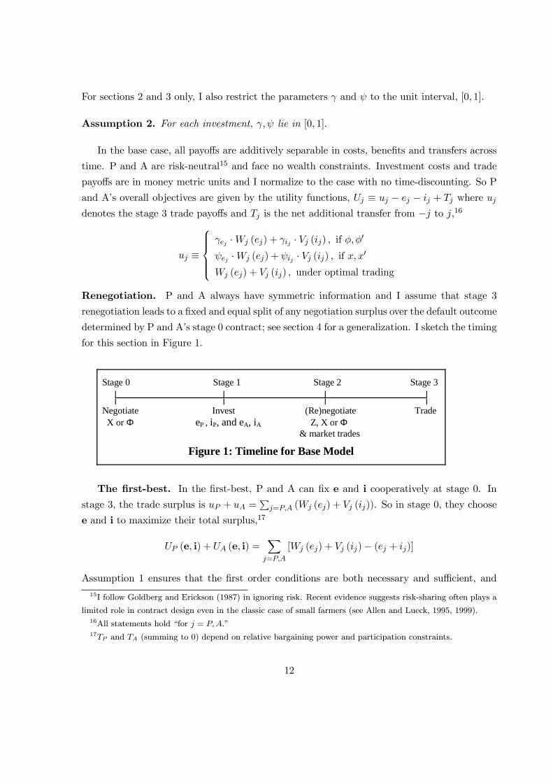
determined by P and A�s stage 0 contract; see section 4 for a generalization. I sketch the timing

for this section in Figure 1.

Stage 0 Stage 1 Stage 2 Stage 3

| | | | Negotiate Invest (Re)negotiate Trade X or Φ eP , iP, and eA, iA Z, X or Φ & market trades

Figure 1: Timeline for Base Model

The Þrst-best. In the Þrst-best, P and A can Þx e and i cooperatively at stage 0. In

stage 3, the trade surplus is uP + uA =Pj=P,A (Wj (ej) + Vj (ij)). So in stage 0, they choose

e and i to maximize their total surplus,17

UP (e, i) + UA (e, i) =Xj=P,A

[Wj (ej) + Vj (ij)− (ej + ij)]

Assumption 1 ensures that the Þrst order conditions are both necessary and sufficient, and

15I follow Goldberg and Erickson (1987) in ignoring risk. Recent evidence suggests risk-sharing often plays a

limited role in contract design even in the classic case of small farmers (see Allen and Lueck, 1995, 1999).16All statements hold �for j = P,A.�17TP and TA (summing to 0) depend on relative bargaining power and participation constraints.

12

give unique solutions to the Þrst-best which I denote with a superscript∗,

V 0j³i∗j´− 1 = 0

W 0j

³e∗j´− 1 = 0 (1)

In the second-best equilibrium, P and A choose e and i non-cooperatively, because these

investments, their costs, and their resulting payoffs u, are all non-veriÞable (e.g., outsiders

cannot measure the quality or cost of IBM�s coaching investments). I therefore compare the

Subgame Perfect Equilibria from alternative feasible stage 0 contracts to derive the optimal

contract. I begin (in 2.1 and 2.2) with the two extreme contracts where P and A choose

either X or Φ at stage 0. Superscripts LTC and STC indicate the equilibrium values from

long-term contracting (choosing X at stage 0) and short-term contracting (choosing Φ at stage

0), respectively. I then treat the general case in 2.3; those familiar with incomplete contract

theory can jump straight to 2.3.

2.1 Equilibrium with long-term contracting

When P and A agree on X at stage 0, their default payoffs in stage 2 renegotiation are given by

the expression, ψej ·Wj (ej)+ψij ·Vj (ij). The total gain available on renegotiation is therefore,Xj=P,A

h³1− ψej

´·Wj (ej) +

³1− ψij

´· Vj (ij)

iP and A each get their default payoffs plus half of these renegotiation gains, so after making

investments e and i, their expected payoffs from stage 2 onwards are given by,

1

2

³1 + ψej

´Wj (ej) +

1

2

³1 + ψij

´Vj (ij) +K (e−j , i−j)

where K (e−j , i−j) ≡ 12

h³1− ψe−j

´·W−j +

³1− ψi−j

´· V−j

i. I solve for the Subgame Perfect

Equilibrium using backward induction. Party j invests to maximize this expected return less

its investment cost, ej + ij. Since K (·) is independent of ej and ij, j�s problem is,

maxej ,ij

µ1

2

³1 + ψej

´Wj (ej) +

1

2

³1 + ψij

´Vj (ij)− (ej + ij)

¶The Þrst order conditions are again necessary and sufficient,

1

2

³1 + ψej

´W 0j (ej)− 1 = 0

1

2

³1 + ψij

´V 0j (ij)− 1 = 0

13

When ψ = 1, these conditions replicate equation (1) and give the Þrst-best, but for ψ < 1,

the concavity of W and V implies underinvestment. Investor j�s investments increase with

j�s share of default returns, which increase with the compatibility parameters, ψej and ψij ;

long-term contracting protects investments to the extent that they are directly compatible or

side-compatible with the contract. The general intuition is familiar: a higher investment return

in the default outcome reduces dependence on negotiating with the speciÞc trading partner.

The investor therefore loses a smaller share of investment returns in renegotiation, and better

internalizes the investment.

Proposition 1. eLTCj rises with ψej and iLTCj rises with ψij . Assumption 2 implies

underinvestment in iP and iA and weak underinvestment in eP and eA : iLTCj < i∗j

and eLTCj ≤ e∗j with equality only when ψej = 1.

2.2 Equilibrium with short-term contracting

When P and A choose Φ at stage 0, their stage 2 default payoffs are given by the expression,

γej · Wj (ej) + γij · Vj (ij). By analogy with the long-term contracting case, the Þrst order

conditions are,

1

2

³1 + γej

´W 0j (ej)− 1 = 0

1

2

³1 + γij

´V 0j (ij)− 1 = 0

Investments now increase with γ instead of ψ, and there is underinvestment when γ < 1.

Proposition 2. eSTCj rises with γej and iSTCj rises with γij . Assumption 2 implies

underinvestment in eP and eA and weak underinvestment in iP and iA : eSTCj < e∗j

and iSTCj ≤ i∗j with equality only when γij = 1.

In words, short-term contracting allows market forces to motivate investments to the extent

that they are general, but (by the classic holdup problem) speciÞcity causes underinvestment.18

2.3 Equilibrium with intermediate contract length

In Section 5, contracts can extend over multiple trading periods, but even in the basic model,

I can treat contract length as a continuous variable by allowing for stochastic enforcement. I

18The intuition again follows from asking whether an investor can appropriate investment returns without

having to renegotiate. Under short-term contracting, the default returns are determined by the investor�s market

alternatives reßected in γ. The problem is that market forces do not motivate speciÞc investments.

14

let α denote the probability that X is enforced (in default of renegotiation). With converse

probability 1 − α, P and A�s default contract is Φ. I assume that P and A can choose any

α ∈ [0, 1] at stage 0 - for instance, by varying contractual ambiguity19 or breach damages (see6.2). This generalizes the above analysis because α = 0 corresponds to short-term contracting

(STC) and α = 1 corresponds to long-term contracting (LTC). I refer to α as contract length

- the contract enforces trade for on average α ·G time units where G, the time elapsing betweenstages 0 and 3, is the common gestation period of the investments. The interpretation of α as

a deterministic contract length is validated in the multi-period model of section 5.

The default payoffs are now convex combinations of those from X and Φ with weights, α

and 1− α, respectively. The Þrst-order conditions are therefore,1

2

³1 + α · ψej + (1− α)γej

´W 0j (ej) = 1

1

2

³1 + α · ψij + (1− α)γij

´V 0j (ij) = 1 (2)

This set of equations allows me to generalize the Þrst two propositions and show how contract

length affects investment incentives as a function of the sign and size of ψ−γ. Raising α shiftsweight from γ onto ψ. This raises H ≡ 1 + α · ψ + (1− α) γ when ψ > γ, and lowers it whenψ < γ. Equations (2) then imply that increasing α increases W 0

j (ej) and decreases V0j (ij), so

ej rises and ij falls (as W and V are concave).

Proposition 3. (a) Increasing contract length raises type 1 and lowers type 2

investments. Mathematically,dej(α)dα > 0,

dij(α)dα < 0. (b) Each investment rises

with γ (strictly if α < 1) and with ψ (strictly if α > 0). (c) With Assumption 2,

underinvestment is the only possible inefficiency.

eSTCj < ej (α) < eLTCj ≤ e∗j and iLTCj < ij (α) < i

STCj ≤ i∗j for all α ∈ (0, 1)

This captures the key tradeoff between increasing contract length to protect type 1 investments

and reducing contract length so that market forces can better motivate type 2 investments.

Type 1 investments, eP and eA, are speciÞc but contract-compatible (γ < ψ) so the contract

protects them better than do market forces. Type 2 investments, iP and iA, are general

and contract-incompatible (γ > ψ) so for them, market forces are better than the long-term

contract (with its side-compatible market forces). In the next section, I predict contract length

by trading off contractual protection of e against its cost in shielding out contract-incompatible

market forces that reward i.

19I can redeÞne α to be P and A�s prior estimate of whether stage 3 trade will be induced.

15

3 Optimal Contract Length in the Basic Model

P and A choose contract length at stage 0. In this section, I show how optimal length is

determined by the relative importance of different investments and the effectiveness and com-

patibility of contracts and market forces. In stage 0 negotiations, P and A can use up-front

transfers to share any gains from a surplus increasing contract. So they choose α to maximize

their total surplus, subject (unlike in the Þrst-best) to the �incentive compatibility� conditions

(2) on e and i. I denote the unique solutions of (2) by ej = ej (α) and ij = ij (α). So P and

A�s problem is,

maxα

Xj=P,A

(Wj (ej (α)) + Vj (ij (α))− (ej (α) + ij (α))) (3)

Propositions 1-3 show that underinvestment is the only efficiency problem in the basic

model. Proposition 3 also shows how to motivate more investment: increase α to improve type

1 investments, e, and decrease α to improve type 2 investments, i. Intuition therefore suggests

that α should increase with the importance of eP and eA relative to iP and iA. To investigate

formally, I scale up the payoff impact of investments ej, ij by the importance parameters, Ej ,

Ij > 0 - i.e., I replace ej and Wj (ej) by Ejej and Ej ·Wj (ej) and I replace ij and Vj (ij) by

Ijij and Ij · Vj (ij). Notice that this rescaling does not change the Þrst-order conditions fore and i, but it does change the importance of having e and i close to their Þrst-best levels

(because the surplus loss from underinvestment is increasing in E and I, respectively). The

intuitive idea follows from solving P and A�s rescaled problem,

maxα

Xj=P,A

[EjWj (ej (α)) + IjVj (ij (α))− (Ejej (α) + Ijij (α))] (4a)

Proposition 4a. Assuming the maximand of (4a) is concave (see appendix for

sufficient conditions), the optimal contract length increases with the importance

of investments of type 1, and decreases with importance of type 2�s: α (E, I) has∂α∂Ej

> 0 and ∂α∂Ij

< 0.

This result is consistent with empirical evidence (see e.g., Brickley et al., 2003) on the

positive correlation between contract length and the importance of non-contractible speciÞc

investments, EA. Empiricists use the size of contractible speciÞc investments as a proxy for

the importance of non-contractible speciÞc investments (EA). This proxy is imperfect but

reasonable, because the two types of investment are strongly complementary. For instance,

when IT outsourcing deals involve a signiÞcant (contractible) transfer of workers and assets

from client to vendor, the complementary investments in retraining and reorganization are

16

largely speciÞc and non-contractible (as in the above IBM example). Furthermore, if the return

on training per worker is independent of the transfer size (number of workers transferred), the

total training investment and its return can be written asEe andE·W (e); the rescaling exercise

then exactly captures variation in transfer size. Using transfer size as a proxy, proposition 4

readily explains why almost all the longer IT contracts (those over 5 years long) occur in these

�merger and acquisition� type deals.

An alternative comparative static exercise is to vary the productivity of an investment, so

that ej generates a return �Ej ·Wj (ej) and similarly for ij with productivity parameter �Ij . This

changes the Þrst-order conditions to,

1

2H³α;ψej , γej

´�Ej ·W 0

j (ej) = 1

1

2H³α;ψij , γij

´�Ij · V 0j (ij) = 1 (5)

where H (α;ψ, γ) ≡ (1 + α · ψ + (1− α)γ)

P and A�s problem is now,

maxα

Xj=P,A

³�Ej ·Wj

³ej³α, �Ej

´´+ �Ij · Vj

³ij³α, �Ij

´´−³ej³α, �Ej

´+ ij

³α, �Ij

´´´(4b)

where ej³α, �Ej

´and ij

³α, �Ij

´solve incentive compatibility conditions (5). Notice that the

productivity parameters raise incentives to invest for Þxed α (i.e.,∂ej(α, �Ej)∂ �Ej

,∂ij(α,�Ij)∂ �Ij

> 0).

This effect countervails against the need to use α to further raise incentives (to exploit the

productivity as in the intuition), so a clear result in this case requires a regularity condition

(familiar from insurance contracting20),

Assumption 3. W 0j (ej)W

000j (ej) >

³W 00j (ej)

´2and V 0j (ij)V 000j (ij) >

³V 00j (ij)

´2, ∀ej , ij.

Proposition 4b. Under assumption 3 (and the regularity condition of Proposition

4a), the optimal contract length increases with the productivity of investments of

type 1, and decreases with productivity of type 2 investments: �E,�I

´has ∂α

∂ �Ej> 0

and ∂α∂ �Ij

< 0.

The effectiveness of markets and contracts (captured by γ and ψ) also affects optimal

contract length. There are two types of effect for any given investment. First, if ψ and

20There is no precautionary saving interpretation here, but consider the sharp countervailing effect of a Þxed

cost self-investment: when the investment�s importance generates incentives exceeding the Þxed cost, α can be

decreased. Assumptions 1 and 3 rule out generalized versions of this problem.

17

γ change so that δ ≡ ψ − γ rises while H (α;ψ, γ) ≡ 1 + α · ψ + (1− α)γ is Þxed, long-term contracting becomes more effective relative to the market forces freed by short-term

contracting. This intuitively favors the use of longer contracts and should increase α. I call

this a substitution effect, because P and A substitute market forces for contract length according

to their relative effectiveness as investment motivators. Second, an increase in γ or ψ directly

raises the investment level for any given α. This level effect is determined by changes in H (α)

for Þxed α and δ. The level effect reduces the need to adjust α in favour of the investment, so

the level effect on α is negative for type 1 investments and positive for type 2 investments.

Proposition 5. (Assume the regularity condition of Proposition 4a.) Contract

length rises when type 1 investments become more speciÞc (γ falls) and falls when

type 2 investments become less contract-compatible (ψ falls). In general: Changes

that increase δ = ψ − γ have a positive �substitution effect:� ∂α(γ,ψ)∂δ |H= �H > 0;

Changes that increase H (α;ψ, γ) have a �level� effect that is negative for type 1,

but positive for type 2, investments: ∂α(γ,ψ)∂H |δ=�δsign= −�δ.

I use two direct corollaries in section 6. First, contract length rises with ψ for type 2 in-

vestments, so raising side-compatibility of an adaptation investment raises optimal contract

length.21 Given that side-compatibility tends to be higher in multi-sourcing, this generates a

tendency for longer contracts in multi-vendor situations. Second, contract length rises when

market alternatives fall, because this makes investments more speciÞc, i.e., γ falls. This claim,

famously supported by Joskow (1987) and others, is clearly valid for type 1 investments. My

model shows that there is a complication, because the level effect when type 2 investments

become more speciÞc could motivate shorter contracts. However, the substitution effects are

positive for all investments, so this effect will only dominate in special cases. Furthermore,

some investments could switch from type 2 to type 1, raising the relative importance of type

1 investments and inducing longer contracts by proposition 4.

4 Cross Effects, Waste and Bargaining Asymmetry

This section extends the model to allow for investment externalities, wasteful investment and

bargaining asymmetries. A cross effect is an investment externality that occurs under the

basic contract X: the basic contract induces a (non-contractible) quality of trade that depends

on prior investment by the trading partner.22 Cross effects may be negative. For instance,

21This generalizes to both investment types if level effects are limited (as when α = 0).22Recall the introductory example where IBM�s storage efficiency raises Amex�s trade value under their pay-

as-you-use contract. A Þxed price contract prevents this cross effect, but then Amex�s server needs have a

18

IBM might develop a way to cut its cost (of satisfying the basic contract) at some expense to

quality (as occurs under privatization in Hart et al., 1997). I deÞne a cross-general effect as an

investment externality occurring under Φ. This occurs when one party�s investment improves

the other party�s market alternatives under Φ. For instance, Amex might learn technical or

marketing knowledge from watching IBM invest in their joint trade.23 To complete the picture,

I allow for negative cross-general effects where an investment harms the trade partner�s market

reputation.

IBM�s private return on a negative cross-investment exceeds the social return, so I allow for

ψ > 1. This case also occurs for speciÞc investments if separate trading is sometimes optimal.

Similarly, γ > 1 when investments (e.g., in advertising or search) generate alternatives that

are mostly used as threat points. To allow for pure threat point investments, I even consider

investments that are entirely wasteful in that their social return is zero. (Such threats - e.g.

to exploit a contractual loophole - are never implemented in equilibrium.)

To extend the model, I now allow j�s investment, ej to raise −j�s payoff by ψcrossej ·Wj (ej)

under X (the cross effect), and by γcrossej ·Wj (ej) under Φ (the cross-general effect). I also

allow ej to be a wasteful investment by removing the additive Wj (ej) term from the trade

surplus under Z.24 Similarly, for ij . The impact of j�s positive cross effects is to reduce j�s

payoff from renegotiation, because −j�s default payoff is increased. The Þrst order conditions(5) are unchanged except that (a) ψ and γ are replaced by ψ ≡ ψ−ψcross and γ ≡ γ − γcross,and (b) in the case of wasteful investments, H (α;ψ, γ) = 1 + α · ψ + (1− α) γ is replaced byH¡α; ψ, γ

¢− 1 = α · ψ + (1− α) γ.The implications of the cross effects are immediate corollaries of propositions 1 to 5 because

all these results continue to hold after substituting ψ and γ in place of ψ and γ (see below on the

case where ψ or γ /∈ [0, 1]). The cross effects simply countervail against the corresponding selfeffects. In particular, an investment increases with contract length if and only if ψ − ψcross >γ−γcross. So the natural extension of the type 1 investment is deÞned by δ ≡ ψ− γ > 0 whiletype 2 investments are deÞned by δ < 0.

A pure cross-investment is one for which ψcross > 0, while the other parameters are zero.

This is a type 2 investment because δ = −ψcross < 0. So cross-investments fall with contractlength α even though there cannot be any market-shielding if γ = 0. Instead, the long-

term contract is costly (as in Che and Hausch, 1999), because it increases the investment�s

cross-effect on IBM (see also 6.1).23Similarly, suppliers may learn from their buyers. E.g., Solectron learned how to make own-brand products

after working for IBM, HP and Mitsubishi (see Arru�nada and Vazquez, 2004, and Lee and Hoyt, 2001).24If ej actually reduces this social return, the effects are simply more pronounced.

19

externality and therefore lowers the investor�s incentive. A corollary of the extended version

of proposition 4 is that contracts should become shorter as cross-investments become more

important.25

A pure cross-general investment is one for which only γcross > 0. This is a type 1 invest-

ment since δ = γcross > 0, so it rises with α. The contract helps because it shields out the

market externality. The extension of proposition 4 predicts longer contracts when cross-general

effects are important. A contract imposing exclusivity alone may (if legal) be more effective

in preventing cross-general externalities (see Segal and Whinston, 2000), but performance

contracting is often preferable since this also motivates self-investments and side-compatible

adaptations.

Asymmetries in bargaining do not change the nature of these effects, but they do change the

relative importance of cross and self effects, because self effects lead to a beneÞt without need

for bargaining power, while cross effects only matter through traders� renegotiation shares. If

j now wins a share θj ∈ [0, 1] of the renegotiation returns, j�s incentive conditions are as in (5)except that (a) ψ and γ replaced by ψ (θ) ≡ (1− θ)ψ− θψcross and γ (θ) ≡ (1− θ)γ − θγcrossand (b) H (α;ψ, γ) is replaced by H (α;ψ, γ, θ) ≡ [2θ + α · ψ (θ) + (1− α)γ (θ)]. Again theresults extend in straightforward fashion. An investment is now type 1 if δ (θ) > 0 where

δ (θ) ≡ ψ (θ) − γ (θ), and type 2 if δ (θ) < 0. I now return to the case with θ = 12 for

expositional ßuidity.

When an investment is wasteful, the impact of contract length is determined by its para-

meters ψ and γ exactly as for productive investments apart from the level effect implicit in

replacing the factor H by H − 1 (H − 2θ in the general case). However, the maximand (3)only includes the subtraction of the investment cost, since it has no social return. So P and

A aim to minimize the cost, and the message of proposition 4 is exactly inverted. I Þrst prove

this in proposition 6a by varying the importance (scale), Kj, of a wasteful investment, kj that

costs Kjkj and generates private returns Kj ·Bj (kj) where Bj (·) satisÞes the above regularityconditions. Then in proposition 6b, I prove the same result holds for increases in the produc-

tivity �Kj of a wasteful investment kj , that costs kj and generates private returns of �KjBj (kj).

This second result requires that Bj (·) satisfy assumption 3, because of the countervailing effectdescribed in proposition 4b above. (Interestingly, assumption 3 is also a sufficient condition

25There is one complication. Intermediate breach penalties might allow the non-investing trader to credibly

threaten termination after low cross-investment. Che and Hausch (1999) argue that such option schemes do not

work (given renegotiation), because the trader would threaten to terminate even after high cross-investment.

Ellman (2006) shows that, absent reputational mechanisms, this critique is invalid when options are decided by

a trading decision (see also Watson, 2005). However, option schemes have α < 1 in generic stochastic settings,

so there is still a tendency towards shorter contracts.

20

for regularity (concavity) of the overall maximization problem.)

Proposition 6a. Optimal contract length is decreasing in the importance of any

wasteful type 1 investment with return function satisfying assumption 1 and reg-

ularity of the overall optimization - assumption 3 is a sufficient condition. By

contrast, optimal contract length increases with the importance of wasteful type 2

investments: dαdKj

< 0 if and only if δj > 0.

Proposition 6b. If a wasteful investment�s return function satisÞes assumptions

1 and 3, optimal contract length is decreasing in the investment� productivity for

type 1 investments and increasing in productivity for type 2 investments: dαd �Kj

< 0

if and only if δj > 0.

When ψ > 1 (either from negative cross-investment effects or from ψ > 1 or both), there

is a risk of over-investment - for any α > 1−γψ−γ . So, for high α, changing the productivity

(importance) of this investment has the same effect as if the investment were wasteful, while

for low α, the implications are as in proposition 4. Similarly, when γ > 1, there is a risk of

over-investment for low values of α.26

In conclusion, the impact of cross effects (ψcross and γcross) is the inverse of the correspond-

ing self effects (ψ and γ) and the impact of importance on contract length is inverted for an

investment that is wasteful or excessive. When traders are inexperienced or uncertainty and

complexity are high, it is harder to write contracts that pin down quality, so there is a greater

risk of cross effects. This section helps explain why contracts are often short in such settings:

contract length is reduced to better motivate cross-investments and to reduce over-investment

in investments with negative cross effects. (A complementary effect of uncertainty is to increase

the importance of adaptations. This can also explain the shorter contracts observed.)

5 Temporal Extension

This section analyzes multi-period extensions of the trading model. Stage 3 trading is spread

over time27 and subdivided intoN discrete trade decisions, each lasting l units of time. A simple

long-term contract enforcing trade in the Þrstm ≤ N substages has length L = m·l+G (where26To complete the generalization, ψ and γ might also be negative, but this has no special effect other than

possible corner solutions at zero investment.27Trade is often spread over time because production is time-intensive, being limited by capacity and proce-

dural constraints. Also demands are spread over time (and storage is impossible for services like IT). See 6.1 on

endogenizing trade intensity.

21

as deÞned above, G is the time elapsing between stages 0 and 3). In this section, I analyze

why optimal contracts often take this form and show that the tradeoff from varying L is then

identical to that of varying α in the basic model: Increasing L protects self-investments for

longer, but shields out for longer market forces that protect adaptations.

I maintain the standard assumption that parties can always renegotiate, so I need N

renegotiation stages - one before each trading decision. In the simplest extension, there is only

one investment stage and no history dependence within the extended trading interval, so the

trade payoffs in each substage are scalar multiples of the trade payoffs from the basic model.

The impact of stage 1 investments may vary with time, so I let the compatibility, generality

and importance parameters depend on n. The overall game is as before except that stages 2

and 3 are replaced by their N−fold replication and the initial contract determines a probabilityαn of trade enforcement via Xn (equivalent to X) in each of the n trade stages. The extended

timing is therefore: (Stage 0) P and A negotiate (αn)Nn=1 and lump-sum transfers; (Stage 1) P

and A invest; [(Stage 2n) Renegotiation over Xn; (Stage 2n+ 1) n�th trading decisions]n=Nn=1 .

Given the absence of history-dependence within the subgame starting from stage 2,28 the

continuation payoffs equal the sum of the equilibrium payoffs from the N paired stages (2n

and 2n+ 1)n=Nn=1 . The Þrst-order conditions therefore modify (5) into,ÃNXn=1

1

2H¡αn; ψe,j,n, γe,j,n

¢ · �Ej,n!·W 0

j (ej) = 1

ÃNXn=1

1

2H¡αn; ψi,j,n, γi,j,n

¢ · �Ij,n!· V 0j (ij) = 1 (6)

In the case of a time invariant technology, the summations in (6) simplify to 12H¡α; ψi,j, γi,j

¢· �Ejand 1

2H¡α; ψi,j, γi,j

¢ · �Ij , where α ≡ ΣNn=1αnN and �Ej =

PNn=1

�Ej,n (= N · �Ej,n for each n) and�Ij = N · �Ij,n (for all n). So contracts with the same α are equivalent in terms of incentiveefficiency. In particular, the simple long-term contract of length L = m · l is deÞned byαn = 1{n≤m}, so it is equivalent to α = m

N (= L−GL−G where L = N · l is the maximal trade

duration) and I can state,

Proposition 7. In the multi-period extension with time invariance, restricting to

simple long-term contracts has no efficiency cost and propositions 1-6 all hold with

L replacing α.

28Renegotiation and interdependence among the αn could create history-dependence inside the subgame, but

the game with independent αn and renegotiation restricted to only adjusting the contract for the upcoming

trading period has the same equilibria.

22

Time-invariance is a special case. Allowing for variation in the productivity parameters E

and I over time n permits further predictions. First, if self-investments become redundant over

time and/or adaptation investments become more important over time, simple contracts are

uniquely optimal. The intuition is that simple contracts exploit contractual protection where

most effective and least harmful (in terms of market-shielding), because they crowd trade en-

forcement into the earliest substages where Ej,n is large relative to Ij,n.29 Second, one can study

varying gestation periods, by setting G = 0 and deÞning Gej = l ·max {n : Ej,n = 0∀m ≤ n}(and Gij similarly). Two implications are immediate. If contract length L > 0, then L should

exceed minj Gej , because otherwise the contract has no protection beneÞt.30 This may help

explain why agriculture contracts are longer in the case of fruit trees as shown in Bandiera�s

(2002) historical data. However, when Gej gets too large, the market-shielding cost may be

prohibitive and L will fall back, as traders abandon the idea of protecting ej. Further impli-

cations, depend on the time proÞles of investment productivity and can be analyzed using the

extended model.

A pair of arguably stronger reasons for the prevalence of simple contracts derive from plau-

sible history dependence within the trade interval. Unless a contract is simple, it must involve

at least one �performance gap� during which the contract does not enforce joint trade. Switch-

ing to an alternative trade during such a gap is often not credible, because the trader would

anticipate having to pay Þxed costs of switching back to joint trade after the gap (in addition to

Þxed costs of switching to the alternative trade).31 This implies market-shielding even during

the contractual gap, so there is no cost from Þlling in the gap with performance. Even when

switching is credible during a gap (that is long enough to justify the Þxed costs of switching)

switching to an alternative partner for the main trade can reduce the marginal value of speciÞc

investments when returning to joint trade. For instance, switching may require reorganiza-

tions that interfere with the speciÞc investments. This reduces the effectiveness (investment

protection) of imposing performance after the gap. With these endogenous parameter shifts,

avoiding performance gaps through simple contracts is optimal since it maximizes contract

29The general condition for unique optimality of simple contracts is that the importance of type 1 investments

grow at a lower rate than for type 2�s - i.e., εn ≡ �Ej,n+1�Ej,n

< ιn ≡ �Ij,n+1�Ij,n

,∀n,∀j. The proof is simple when γ andψ are independent of n: The summation terms in the Þrst-order conditions become 1

2H¡PN

n=1αn �Ej,n; ψej , γej

¢and 1

2H¡PN

n=1αn �Ij,n; ψij , γij

¢. Now suppose that αn+1 > 0 when αn < 1. Decreasing αn+1 by (any feasible)

η > 0 and increasing αn by ιn · η Þxes the incentive on all type 2 investments and increases the incentives for alltype 1 investments by (ιn − εn) η2 δ > 0. Hence �αn < 1⇒ �αn+1 = 0 ∀n ∈ {1, 2, ..., N}. Gaps are always avoided.30If minj Gij > 0 then there is no market-shielding cost for L ∈ [0,minj Gij ) so the precise claim is that L

should exceed minj Gej , if L > minj Gij .31For side-compatible adaptations, alternative trade credibility is in fact higher during performance

contracting.

23

protection relative to market-shielding.32

My model could be extended in two directions. First, I have deferred a general analysis

of settings with switching costs, because intermediate breach penalties can generate a rich

multiplicity of equilibria. In this case, alternative trades become �outside options� (see Osborne

and Rubinstein (1990)). If one applies the Outside Option Principle as in MacLeod and

Malcomson (1993), my results apply unless one trader�s outside option binds in which case the

other trader gets the full share of renegotiation surplus. If only one trader makes relationship-

speciÞc investments, the tradeoff between protection and market forces is escaped by giving

an attractive breach option to the trader who only makes general investments.

Second, initial investments are often the most important - as with IBM�s training invest-

ments - however, ongoing investments are also important, especially for adaptations. Intro-

ducing additional investment stages after stage 2 requires ongoing renegotiation in which the

new contract at each stage should be designed to optimize incentives for the upcoming invest-

ment problem. My framework would then predict the length of each new contract, assuming

intertemporal additivity for all investments. Guriev and Kvassov (2006) study precisely this

problem in the case of a single investment, though without the market-shielding problem, and

under the premise that renegotiation is exogenously costly.33

However, I suspect that these predictions are sensitive to the symmetric information as-

sumption. For instance, the long Þxed term in the IBM-Amex contract was mostly driven by

the need to motivate early investments in reorganization and retraining. Introducing ongo-

ing adaptation investments (or cross-investments), one might have expected renegotiation to

a shorter contract once IBM�s main transition costs had been sunk. This has not happened

so far and such renegotiations are rare. I suggest two reasons. First, asymmetric information

frustrates such renegotiation. When unable to fully observe IBM�s training investments, Amex

faces an adverse selection problem, because IBM is more willing to shorten the contract after

weak training investments. Furthermore, renegotiation terms cannot depend fully on IBM�s

training investments, so IBM�s incentives would suffer greatly. Second, the remaining length of

32I defer a general analysis of settings with switching costs, because intermediate breach penalties can generate

a rich multiplicity of equilibria. Alternative trades become �outside options� (see Osborne and Rubinstein

(1990)). If one applies the Outside Option Principle as in MacLeod and Malcomson (1993), my results apply

unless one trader�s outside option binds in which case the other trader gets the full share of renegotiation surplus.

If only one trader makes relationship-speciÞc investments, the tradeoff between protection and market forces is

escaped by giving an attractive breach option to the trader who only makes general investments.33They show how contracts specifying a minimum advance notice for termination provide ongoing investment

incentives without need for continuous renegotiation. Adding my market-shielding effect to their problem would

lead to shorter advance notice requirements. Che and Sakovicz (2004) also allow for ongoing investment, but

assume trade can only occur once and focus on an inÞnite time horizon.

24

the contract and size of breach penalties fall automatically with time, so adaptation incentives

automatically increase over time.

I conclude this section with a brief comment on measuring contract length. This is non-

trivial when breach is stochastic (as in 6.2). I deÞned the �effective� length of a contract as the

amount of time over which a single performance contract would induce trade in the absence

of renegotiation. Through premature breach, this can be lower than the length reported in

the contract (called the �nominal� length in Aghion and Bolton, 1987). Nonetheless, reported

nominal length (7 years in the case of IBM-Amex) is a good proxy for effective length, because

breach penalties often fall sharply to zero at the end of the reported period.34

6 Applications

This section describes how contractual features (quantity decisions, various types of menu,

contractual restrictions, breach damages and informal enforcement) and trading choices (multi-

sourcing, capacity dedication and selective outsourcing) affect the compatibility parameter ψ

and market-shielding. In particular, the last three subsections analyze the empirical puzzles

from the introduction. My examples remain focused on IT outsourcing and I refer to the Cen-

ter for Organizations Research and Innovation (CORI) for detailed IT outsourcing contracts:

Cobancorp-EDS (1995-2002), UHS-Unisys (1996-2005), GM-EDS (1996-2006), Tri City Bank-

M&I Data Services (1998-2006). However, I also use data on the multi-year contracts in

contract manufacturing, input procurement and franchising.

6.1 Contract Design

Three minor extensions of the basic model greatly increase the realism. First, traders generally

choose among many possible basic trades when writing their initial performance contract. The

traders then optimally choose a contract with which valuable investments are highly compatible

and undesirable investments have zero or low compatibility.35 It is instructive to revisit Edlin

and Reichelstein�s (1996) model of self-investments in which speciÞc performance contracts

with carefully chosen trade quantity can induce Þrst-best investment incentives. Introducing

adaptation investments into their model would prevent reaching the Þrst-best, because raising

trade quantity (or intensity) reduces side-compatibility (see model of the intensity variable

denoted d in section 2 and in 6.4 below). In the multi-period model laid out in section 5, an

34For ever-green contracts, the length of the advance notice period is the key proxy, but the size of the penalty

on giving notice is particularly important as the effective length is inÞnite if this penalty is too high.35This statement applies with opposite signs for cross compatibility.

25

extremely brief but intense contract could conceivably limit this market-shielding problem, but

there is a major risk that such a contract would simply encourage wasteful investments that

are only useful for producing at artiÞcially high intensity.

Second, the long-term contract might include a trade menu from which at least one party

(usually the client) can choose after investing. For instance, in IBM and Amex�s �pay-as-you-

use� contract, Amex owes less to IBM if it uses less server space. This raises side-compatibility

for any Amex adaptation that affects its server space needs. However, ßexibility must be limited

to protect the seller�s speciÞc investments. Pricing is generally non-linear. For instance, the

lion�s share of Amex�s service charge is effectively Þxed.36

Third, the contractual menu might be determined over time through a set of modiÞcation

procedures. Indeed, a large share of vendor compensation in the long-term contracts supporting

�acquisition� deals (involving substantial restructuring as in Amex�IBM) comes in the form

of a �revenue commitment� that Þxes a minimal expenditure by the client on the vendor�s

services (sometimes, as a percentage of the client�s IT expenditure - see GM�EDS, 1996).

Revenue commitments give the client the ßexibility to choose what to buy, but this ßexibility

is only meaningful when optional items are reasonably priced. Arbitration and benchmarking

procedures are therefore necessary. These procedures work well for minor modiÞcations and

easily priced �new releases,� but there is a signiÞcant risk that the arbitrator (being imperfectly

informed) speciÞes an excessive price on a non-standard adaptation or additional service. The

vendor and client then engage in bilateral negotiations to Þnd a mutually agreeable price. So

the credibility of market threats again determines the degree of holdup.37 Any changes that

require negotiation are equivalent to adaptations and my analysis continues to apply.38

Cost-plus contracts can be viewed as a menu contract in which they buyer can demand

adaptations on the condition of paying the additional costs required by adaptation. When

containing a minimal trade guarantee, such a contract is very similar to the revenue commit-

ment contract. In ideal circumstances, this again resolves the holdup problems analyzed above.

36Koch (2003) criticizes IBM�s exaggeration in claiming to have invented a fully ßexible �e-business utility�

model. Goldberg and Erickson (1987) is a classic reference on non-linearity in long-term contracting.37Arbitrators may require demonstration of market alternatives when seeking benchmark prices. The credi-

bility of side-trading then affects the benchmarked price Þxed by this �market test.� See e.g., additional services

and market tests in GM-EDS�s $40bn contract.38Relatedly, some contracts Þx an annual limit on �system enhancements� that the client can demand at a

predetermined total price, but again the arbitrator�s ignorance may lead to over-estimates of the work hours

required for a given enhancement. Flexibility is further limited when the client exceeds the �total work hours�

as occurred to the UK Inland Revenue�Accenture contract after legislators introduced �stakeholder pensions�

in 1998 and quarterly tax reporting for corporations in 1999 (see NAO, 2001).

26

However, the problem is as before: measuring adaptation costs is often too difficult.39

6.2 Contract Enforcement and Breach Damages

As just noted, the principal contract enforcement problem underlying my main result is the

non-veriÞability of adaptation costs. Since veriÞability is also a problem for informal enforce-

ment mechanisms involving third parties, my results continue to apply in settings where trade

agreements are enforced by group or market reputations. However, if the trading relationship

were governed by bilateral self-enforcement (also called relational contracting), these informa-

tional constraints would be avoided. Unfortunately, in settings where large speciÞc investments

are sunk at the start of the relationship and pay off over a period of many years, repetition

within the same relationship is unlikely. So self-enforcement of these investments is not usually

feasible. By contrast, adaptation investments and returns are often more frequently repeated,

so reputational mechanisms should favour longer contracts.40

My sharp non-veriÞability assumptions also ruled out more subtle breach penalties such

as reliance and expectation damage measures as alternatives to liquidated damages. Relaxing

these assumptions reduces the difficulty of motivating investments, but with imperfect measure-

ment of the potential costs and beneÞts from adaptation, market forces and side-compatibility

still matter. Even without relaxing the assumptions, there is one further issue: the optimal

contract design may involve intermediate liquidated damages.

In section 4, I explained how intermediate damages enable option contracts to induce

breach threats after low cross-investment. I now show how intermediate damages can make

breach credibility contingent on the stochastic value of adaptation investments. For instance,

after Halifax acquired the Bank of Scotland (BoS) in 2002, its gain from substituting BoS�s

centralized IT infrastructure with a more decentralized system exceeded the breach damages

in BoS�s outsourcing contracts with IBM and Xansa (see Computer Weekly, 2002). So the

acquisition induced breach and the marginal returns on acquisition investments were high, be-

cause the breach penalty was fairly low. In terms of the model, the moderate breach penalties

39My strict assumption that costs are non-veriÞable rules out cost-plus contracting, but in settings where

many similar traders could gain from long-term contracting and good incentives to adapt, the traders might

pay to create a specialist agency that would build a capability and reputation for verifying adaptation costs.

In these settings, contracts could be longer without suffering from serious rigidities. (Of course, if the agency

could also verify investments, long-term contracts would not be needed either.)40SpeciÞc assumptions about renegotiation are also important. For instance, they determine whether long-

term contracts can credibly increase mutual punishment in support of self-enforcement. (For evidence that

formality does not imply deep distrust, notice that the litigation between Xerox and EDS did not prevent them

from later extending their trading relationship � DiSabatino, 2001).

27

raised side-compatibility without an excessive fall in protection of self-investments. In gen-

eral, it is optimal to make breach credible in states where the marginal returns to adaptation

investments are maximal, thereby exploiting market forces at their most powerful. Interme-

diate breach damages therefore dominate stochastic enforcement with high breach penalties,

whenever the marginal and absolute returns on adaptations are positively correlated.41

6.3 Multiple Vendors

In 2003, Procter and Gamble (P&G) decided against putting all its eggs in one basket, by

outsourcing its IT to three key vendors: Hewlett-Packard, IBM and Jones, Lang & Lasalle �

see Weiss and Perez (2003). A stylized analysis of this decision clariÞes the ßexibility advantage

of the multi-vendor approach; see Currie (1998) for two related case studies. Each vendor had

to sink Þxed costs in learning about P&G. Had P&G instead outsourced to EDS in a one-stop

contract, as initially planned, EDS would have reaped economies of scope by sinking one set,

instead of three sets, of Þxed learning costs. However, in addition to minor specialization

gains, P&G beneÞts from the multiple sunk costs, because these three vendors create credible

competition for many of the service adaptations that P&G may later discover (see model

below). This increased competition allows P&G to negotiate adaptations more cheaply and

more reliably.

Lopez and Ventura (2001) and Gonzalez and Lopez (2002) analyze outsourcing contracts

in the electronics industry using primary source data from ANIEL.42 Their survey reports how

many subcontractors are used by each manufacturer as well as the estimated length of writ-

ten contracts. Having multiple subcontractors, or vendors, is a good proxy for the existence

of competing providers. So, based on Joskow (1987) (see section 3 above), they expected a

negative correlation with contract length. Instead, they found an insigniÞcant positive corre-

lation. I claim that the concept of side-compatibility can resolve this puzzle;43 Multi-sourcing

increases side-compatibility and proposition 5 shows that optimal contract length should there-

fore increase. This counteracts the pressure to make contracts shorter. So it could explain the

41Of course, where possible, breach damages are directly contingent on events � e.g., mergers and acquisitions

� where adaptations tend to be important. Similarly, because adaptations often become increasingly important

over time, breach damages usually fall gradually over the duration of a contract.42Asociacion Nacional de Industrias Electronicas y de Telecomunicaciones. Electronics outsourcing is a global

phenonomenon: e.g., huge 3-year deals between IBM and Sanmina-SCI in 2002 and 2003, and Casio and

Flextronics in 2002, and 5-year deals between HP and Solectron in 2003 and Avaya and Celestica in 2001.43Errors in measurement and coding (of contract length) could also explain the insigniÞcance, so further

empirics is needed. For richer but sparser data with the same positive correlation, see Beulen and Ribbers�

(2003) IT outsourcing case studies.

28

empirical result, but to be thorough, I need to endogenize the sourcing decision. I do so now

for a single buyer with two potential sellers.

I build on the simple technological setup described in the italicized derivation of side-

compatibility from section 2: I allow for exogenous variation in the size of the Þxed startup

costs and in the investment importance parameters, I and E. Each of the two potential

suppliers faces the same Þxed cost F of servicing the buyer�s speciÞc needs. So dual sourcing

wastes a possible scope economy worth F . This may be partially compensated by specialization

gains, S. So the technological advantage of single sourcing is F −S.44 Now for single sourcing,the supplier that is not selected in advance can still avoid sinking its Þxed cost when an adapted

service is discovered, so given F > γW (e), this supplier will not credibly compete for providing

the adapted service and ψ = 0 < γ.45

By contrast, under dual sourcing, the Þxed costs of each supplier have already been sunk,

so each supplier offers credible competition against the other. By construction, adaptation by

the optimal supplier generates W (e). To allow for gains from learning, I suppose the other

provider generates γ0W (e) with γ0 ≥ γ. If the buyer runs a sourcing auction, side-compatibilityψdual is then equal to γ

0. The buyer�s default adaptation returns are just as high as when thedual source contracts expire, since γdual = γ0 too. So the adaptation cost from long-term

contracting is now zero (−δdual = γdual − ψdual = 0) and more generally is much lower thanunder single sourcing.46

So proposition 5 predicts that exogenously imposing dual sourcing will raise contract length.

I now endogenize the sourcing decision. Up-front transfers (determined in the ex ante com-

petition among suppliers) imply that the buyer chooses the sourcing strategy that maximises

total surplus. So I simply compare the surpluses under dual and single sourcing. Dual sourcing

wastes F − S relative to single sourcing, but raises the equilibrium level of adaptation invest-

ments by an amount ∆e. Since ∆e is increasing in contract length α,47 I analyze the joint

choice of sourcing and length.

I begin with the simple case where F or S varies for some exogenous technological reason.

An increase in F −S directly raises the probability of single sourcing and therefore (by reduc-ing side-compatibility) lowers the expected contract length α. Variation in F − S therefore44Positive F − S is trivial: dual sourcing is then technologically and strategically (for investment incentives)

optimal.45This neglects the possibility of multiple trade technologies, but the analysis readily generalizes since the

Þxed cost sunk under dual sourcing generally induces a more efficient side-trading technology.46Economies of scope in variable costs would imply γdual > ψdual, but −δ is still generally greater under single

sourcing, because the added problem of the Þxed costs is greater relative to an isolated side trade.47Dual sourcing could reduce speciÞcity of speciÞc investments where speciÞcity is caused by Þxed costs. Such

an effect would only reinforce the empirical puzzle.

29

generates a negative correlation between single sourcing and contract length, offering a clear

and simple resolution of the empirical puzzle.

Now I analyze the case where variations in sourcing strategies are driven by variations in

the importance (I and E) of adaptation and speciÞc investments. Consider increasing the

importance E of speciÞc investments. By proposition 4a, it is optimal to raise contract length

α, but when the distortion in adaptation incentives gets high enough (I not too small), it

becomes optimal to shift to dual sourcing. Dual sourcing favours adaptation investments, so

this shift is accompanied by an upwards jump in α. Further increases in E again lead to further

increases in α. It follows immediately that dual sourcing is associated with longer contracts

(greater α).

Variations in the importance of adaptation investments have a less monotonic effect. When

I is very low, it is optimal to focus on protecting speciÞc investments with a long-term contract

and dual-sourcing is suboptimal (in the non-trivial case where F − S > 0). As I rises, α

should fall, except at the point (for large enough E) where I is large enough to justify a

shift to dual sourcing. At this point, α jumps upwards, before continuing to fall with I. The

comparison between the average contract lengths associated with dual and single sourcing

therefore depends on the exact density distribution of I. So the prediction here is ambiguous.

My principal contribution is to show that dual sourcing can (and often but not always, will)

favour long-term contracting and to identify conditions favouring this outcome.

To extend the relevance of this section to applied work, it is also important to recognize

that the side-compatibility advantage of multi-sourcing can sometimes be achieved through

�selective outsourcing,� whereby a client retains a strong internal IT unit. Indeed, Amex

chose this approach. Its internal IT unit credibly competes with IBM to satisfy some of its

adaptation needs, so Amex�s side-compatibility is not so low. See Lacity et al., (1996) for

evidence suggesting that selective outsourcing, like multi-sourcing, increases ßexibility.

6.4 Multiple Clients and Dedication

Transaction cost theorists have thoroughly analyzed the contracts between coal processors and

electric utilities. Expanding on Joskow�s (1987) classic approach, Kerkvliet and Shogren (2001)

measured the fraction of capacity each coal company dedicates to the contract for supplying

coal with its utility partner. They were surprised to Þnd a signiÞcant negative correlation

between this measure of dedication and contract length. This Þnding (which is robust to four

explanation attempts performed by Kerkvliet and Shogren, 2001) is indeed anomalous given

that high dedication plausibly proxies for relationship-speciÞcity which tends to require longer

contracts.

30

The side-compatibility perspective offers a simple explanation.48 High dedication to a

speciÞc contract leaves the vendor with less capacity to exploit its adaptations in side-trading,

so side-compatibility is low and this induces shorter contracts (proposition 5). To complete

this explanation, I consider three ways to endogenize the level of dedication. First, as noted in

6.1, increasing a coal company�s supply commitment eventually induces wasteful investments in

capability to satisfy the commitment. An exogenous increase in the distortionary effect of such

commitments (e.g., increased difficulty in predicting output) encourage reduced commitment,

so the fraction of available capacity dedicated to a contract (d) falls. This increases side-

compatibility as explained in section 2 and therefore facilitates an increase in α. Accordingly

α and d are negatively correlated, as claimed. Second, if side-trading involves Þxed costs and

becomes untenable for d above a cut-off level �d, exogenous reductions in �d lead to reductions in d

(assuming adaptations and self-investments are both important). To maintain self-investments,

α can and should then be raised to compensate for the fall in d. So exogenous shifts in �d can also

explain the negative correlation. A third argument follows from the section 5 observation that

when adaptation values increase rapidly over time, it is better to use short, but high intensity

(dedicated) contracts. So variation in the rate of technical change or supply uncertainty could

similarly generate a negative correlation between length and dedication.49

6.5 Contractual Restrictions

In my basic model, long-term contracts impose trade obligations without shifting residual

control rights, but rights and restrictions are sometimes needed to complement performance

contracts. For instance, exclusive territory clauses in a franchise contract (that prevents holdup

through increases in the royalty rate) prevent franchisors from holding up franchisees by setting

up new units that would compete nearby. As complementary tools for protecting speciÞc invest-

ments by franchisees, exclusive territories and contract length should be correlated. Bercovitz

(2000) tests for a positive correlation (her fourth hypothesis, H4) in her rich franchising data

48An alternative is to argue that contract dedication may proxy for coal vendors that have only one client

and therefore (having only paid one set of client-speciÞc Þxed costs) have relatively low side-compatibility.

By analogy with multi-sourcing, exogenous variation in client-speciÞc Þxed costs or the importance of speciÞc

investments could explain a positive correlation between contract length and selling to multiple clients. (I

focus on the simpler explanation in the text, since Kerkvliet and Shogren (2001) measure dedication relative to

available capacity, subtracting prior contractual commitments, so a follow-up study might well Þnd that high

dedication is not a good proxy for having only one client in their dataset.)49Also, uncertainty in electricity demand is greater over longer time horizons, so risk averse utilities may

prefer to buy coal in shorter term contracts as a way to share demand risk with coal producers. Again, contract

dedication would covary negatively to counterbalance length reductions.

31

set. The puzzle is that she Þnds no signiÞcant correlation. The side-compatibility perspec-

tive offers a simple resolution. Exclusivity clauses reduce the side-compatibility of franchisor

investments that require local adaptations, and this makes contract length more costly. Fran-

chise contracts do not always need exclusivity to complement them and (by proposition 5)

contracts will be longer in these cases. For instance, in low density markets, the franchisor

cannot credibly threaten to hold up the franchisee by setting up a new franchise or company

unit nearby, so exclusive territories are not needed. Holdup is adequately prevented by the

long-term franchise contract Þxing royalty rate and fees. However, in denser local markets,

exclusivity territories are needed to complement the long-term contract; incentives for fran-

chisor adaptations are then at risk and contracts should be shorter.50 This offers a reasonable

explanation for the negative correlation.

Interestingly, Bercovitz (2000) also Þnds an insigniÞcant correlation between exclusivity

and her proxy for speciÞcity (franchisor estimates of franchisee set-up costs). Measurement

error might explain the insigniÞcant correlation, but the proxy speciÞcity has been successful

in other work � see Dnes (1992) and Brickley et al., (2003) (which, as mentioned above, con-

tains strong results supporting proposition 4a). Instead, I offer an explanation based on side-

compatibility and the section 5 idea that adaptation investments become more productive over

time. When speciÞcity is low, contracts can be short and exclusivity is a sensible complement

to the contract, since each party can earn a reasonable return on its adaptation investments

by waiting till the contract expires. Exclusivity is problematic, however, when speciÞcity is

important enough to require longer contracts. This countervails against Bercovitz�s prediction

that exclusivity would be more common where speciÞc investments are more signiÞcant.51

Contracts regularly seek the very opposite of exclusivity restrictions, by specifying rights

to solicit competitive bids on services beyond the baseline contract.52 Additionally, IT con-

tracts and industry norms often require standardization and documentation of code, even

pressuring providers to cooperate.53 Further work could extend my model of contracting and

50Kaufmann�s (1993) Harvard Business case study offers a concrete example of an adaptation problem: Pizza

Hut�s efforts to develop and implement a Pepsi promotion scheme through home deliveries were frustrated when

Pizza Hut had to negotiate with franchisees who preferred to focus on eat-in dining.51Future empirical work that identiÞes an exogenous source of variation in the use of exclusivity clauses would

offer an excellent way to test my theory more directly. Variation in the legality of exclusivity restrictions across

U.S. states presents a promising avenue, but restrictive states also tend to restrict contract termination making

reported contract length a biased proxy of contract length.52This was common in Goldberg and Erickson�s (1987) data on coke supply contracts. It is also very common

in IT contracting.53E.g., clause 3.05 in UHS-Unisys obliges Unisys to support third-party software purchased by UHS. Enforce-

ment, however, is difficult � Lacity and Willcocks (1998) report two cases where vendors prevented third-party

32

side-compatibility to analyze how to assign ownership rights when some investments are partly

asset-speciÞc.

7 Concluding Discussion

I have analyzed the optimal duration of performance contracting in a bilateral model where

both traders make multiple investments. My most important result is that contracts should be

shorter when side-compatibility is low and it is important to motivate adaptation investments.

By showing that side-compatibility is high in three relevant settings (when a trader has multiple

vendors, when long-term contracts do not exhaust the capacity or need for trade, and when

there are no exclusivity clauses restricting side-trades), I was able to apply this result to predict

a pressure towards longer contracts and resolve the three empirical puzzles from the transaction

cost literature.

My market-shielding perspective endogenizes and qualiÞes the transaction cost idea that

long-term contracts have ßexibility costs. Formally, I have shown that (unless fully side-

compatible) adaptations can be more cheaply implemented under short-term than long-term

contracting. My framework also indicates why renegotiating from a long-term contract is likely

to be harder than negotiating from scratch:54 competitive bids can reveal information about the

cost of adaptations, reducing information asymmetries and with them, the risk of negotiation

failure, so long-term contracts that reduce competition (because of limited side-compatibility)

increase the risk of failing to negotiate efficient adaptations ex post.55

Because of a false presumption that general investments are not at risk of holdup, other

formal analyses have neglected how long-term contracts interfere with valuable market forces.

Most papers with long-term contracting simply ignored general investments. MacLeod and

Malcomson (1993) is an exception, but they only studied one joint trade, thereby precluding

the possibility of general investments that require an adapted joint trade. The closest analogy

to my market-shielding result is in fact Hart and Moore�s (1990) analysis of ownership. In a

setting without long-term contracting, they showed how removing ownership rights interferes

with access to market forces that could otherwise motivate asset-speciÞc investments. In a

setting with long-term contracts, I have shown how a contractual trading obligation shields

out market forces that could otherwise motivate adaptation investments.

supply by claiming interference with their maintenance obligations. Standards are perhaps more important for

reducing transition costs than side-compatibility � see Beulen and Ribbers (2003).54Many theorists have assumed there is no difference, positing instead an exogenous cost of renegotiation (see

e.g., Harris and Holmstrom, 1987, and Guriev and Kvassov, 2006).55Future work must extend the model to include alternative traders who invest and bid to win new trades.

33

My results formally corroborate prior insights from transaction cost theory on the impact

of market-thickness, investment speciÞcity, contract effectiveness and uncertainty, and novel

results, such as the distinction between the level and substitution effects of changes on contract

length and their dependence on the type of investment. Because the model is very tractable

(for instance, cross effects and wasteful investments have the exact inverse impact of the

corresponding self effects and non-wasteful investments), it is also easy to analyze temporal

variation in investment productivity and future work can extend my multi-period setting to

allow for richer history-dependence.

In the extensions section, I explained how intermediate breach penalties and menu contracts

can raise contractual ßexibility. Relational contracting may further enhance the effectiveness

of menu contracts, so building on the modeling approach of Baker et al., (2002) presents

important work for future analysis. Extending the model to allow for partially measurable

costs is also interesting: Bajari and Tadelis (2001) argue that cost-plus contracts are more

ßexible than Þxed-price contracts because renegotiation is then more efficient. Since Bajari

and Tadelis (2001) do not consider market forces, combining our models could generate novel

predictions. For instance, I conjecture that settings with high side-compatibility will favor

Þxed-price contracting, since these settings limit the inßexibility concern.

In conclusion, the resolution of the three puzzles and the consistency with the evidence

from the transaction cost literature on contract length offers encouraging support for my simple

model. Nonetheless, it is vital to now collect empirical data with an eye to creating effective

proxies of side-compatibility and the other parameters used to predict contract length. This

will permit sharper tests of the model�s predictions and improve our ability to explain the

design and duration of contracts.

34

Appendix

Proof of Proposition 3. Differentiating the identities in (2) with respect to α and deÞning

δej ≡ ψej − γej ,dejdα

=

"−W 0j (ej)

W 00j (ej)

#ψej − γej

1 + α · ψej + (1− α) γej=

−δejW 0j (ej)

H³α;ψej , γej

´W 00j (ej)

(A1)

dijdα

=

"−V 0j (ij)V 00j (ij)

#ψij − γij

1 + α · ψij + (1− α)γij=

−δejV 0j (ij)H³α;ψij , γij

´V 00j (ij)

The bracketed expressions are positive by Assumption 1. H is always positive by Assumption

2. The sign of δ is positive for eP and eA and negative for iP and iA, by type 1 and 2 deÞnitions.

This proves 3(a).

Differentiating with respect to γ and ψ gives,

dejdγej

=

"−W 0j (ej)

W 00j (ej)

#1− α

H³α;ψej , γej

´dejdψej

=

"−W 0j (ej)

W 00j (ej)

#α

H³α;ψej , γej

´Both these expressions are positive for α ∈ (0, 1). The Þrst is positive even when α = 0, thesecond is positive even when α = 1. This proves 3(b) since the exact same expressions and

observations are valid for ij. 3(c) follows from the observations that ej (1) = eLTCj ≤ e∗j and

ij (0) = iSTCj ≤ i∗j - compare Þrst order conditions (2) at α = 1 and 0 with Þrst-best conditions

(1).

Sufficient conditions for concavity (in α) of the maximands in (4a) and (4b):

W 000j W

0j < 4

³W 00j

´2and V 000j V 0j < 4

³V 00j´2

For instance, W and V can take any of the forms,√e, −1e and log e).

Proof of sufficiency. The derivative of the maximand in (4a) is,

D ≡Xj=P,A

ÃEj³W 0j (ej (α))− 1

´e0j (α)| {z }+ Ij

³V 0j (ij (α))− 1

´i0j (α)| {z }

!(A2)

=Xj=P,A

³Dej + Dij

´Differentiating the Þrst component with respect to α again gives,

dDejdα

=d

dα

³Ej³W 0j (ej (α))− 1

´e0j (α)

´= Ej

µW 00j (ej (α))

³e0j (α)

´2+³W 0j (ej (α))− 1

´e00j (α)

¶

35

Now, by (2), 12H³α;ψej , γej

´W 0j (ej) = 1 holds for all α, and H 0 (α) = δej , so δejW

0j (ej) +

HW 00j (ej) e

0j (α) = 0 and,

2δejW00j (ej) e

0j (α) +H

³W 000j (ej) e

0j (α)

2 +W 00j (ej) e

00j (α)

´= 0

So substituting for

e0j (α) =−δejW 0

j (ej)

HW 00j (ej)

=−2δej

H2W 00j (ej)

; e00j (α) =−e0j (α)HW 00

j (ej)

³2δejW

00j (ej)−HW 000

j (ej) e0j (α)

´

dDejdα

=Eje

0j

HW 00j

µH³W 00j

´2e0j +

³W 0j − 1

´³HW 000

j e0j − 2δejW 00

j

´¶

=Eje

0j

HW 00j

Ã−δejW 00

j W0j +

³W 0j − 1

´Ã−δejW

0W 000j

W 00j

− 2δejW 00j

!!

= −δejEje0j

H

W 0j +

³W 0j − 1

´W 0W 000j³

W 00j

´2 + 2

= −δejEje0j

H2

(6− 2H) + (2−H)W 0W 000j³

W 00j

´2

Since e0j, δej , Ej > 0, this expression is negative provided thatW 0W 000

j

(W 00j )

2 <6−2H2−H for all α. Since

H ∈ [1, 2], 6−2H2−H ≥ 4, hence W 0W 000j < 4

³W 00j

´2is clearly sufficient. The term from

dDijdα is also

positive under the parallel condition, because while δij and i0j are both negative, their product

is still positive. This proves that dDdα < 0 for 4a.

Sufficiency for the maximand in 4b follows immediately, because setting E and I to unity

and rescaling W and V by �E and �I does not affect the ratios,W 0W 000

j

(W 00j )

2 andV 000j V 0j(V 00j )

2 .

Proof of Proposition 4a. The Þrst-order condition for the optimization problem (4a) is

D (E, I;α (E, I)) = 0, for D as deÞned in (A2). This holds for all E and I, so applying the

Implicit Function Theorem reveals,

dα

dEj=− ∂D∂Ej∂D∂α

(A3)

∂D∂α < 0 by assumption of concavity (see above for sufficient conditions).

∂D

∂Ej=∂Dej∂Ej

=³W 0j (ej (α))− 1

´e0j (αj) =

µ2

H− 1

¶e0j (α)

36

which is positive since 0 < H < 2 and e0j (α) > 0. Hence dαdEj

> 0. By contrast, dαdIj =

−( 2H−1)i0j(α)∂D∂α

< 0 since i0j (α) < 0.Proof of Proposition 4b. This is slightly more complex, since e and i now depend on E and

I: ej³α, �Ej

´and ij

³α, �Ij

´are such that H �EjW

0j

³ej³α, �Ej

´´= 2, H �IjV

0j

³ij³α, �Ij

´´= 2. So

differentiating, replaces equation (A1) with,∂ej(α,Ej)

∂α =−δejW 0

j(ej , �Ej)HW 00

j (ej , �Ej)=

−2δej�EjH2W 00

j (ej(α, �Ej))(and

a similar expression for ij). The derivative of the maximand in (4b) is,

�D ≡Xj=P,A

ó�EjW

0j

³ej³α, �Ej

´´− 1

´e0j³α, �Ej

´| {z }+

³�IjV

0j

³ij³α, �Ij

´´− 1

´i0j³α, �Ij

´| {z }

!(A4)

=Xj=P,A

³�Dej + �Dij

´So,

∂ �D

∂ �Ej=

∂ �Dej

∂ �Ej=

∂

∂ �Ej

µ 2H− 1

¶ −2δej�EjH2W 00

j

³ej³α, �Ej

´´

=2

H2

µ2

H− 1

¶δej

∂

∂ �Ej

−1�EjW 00

j

³ej³α, �Ej

´´

As H < 2 by assumption 1 and δej > 0 by deÞnition of type 1, this has the same sign as∂∂ �Ej

³�EjW

00j

³ej³α, �Ej

´´´. Differentiating (5) (12H

³α;ψej , γej

´�Ej ·W 0

j

³ej³α, �Ej

´´≡ 1) with

respect to �Ej and substituting shows that,

∂

∂ �Ej

³�EjW

00j

³ej³α, �Ej

´´´=W 00

j + �EjW000j

∂ej

∂ �Ej=W 00

j + �EjW000j

−W 0j

�EjW 00j

As W 00j < 0 by assumption 1, this has the same sign as W

0jW

000j −

³W 00j

´2which is positive by

assumption 3. Hence, ∂D∂ �Ej

> 0 so (A2) reveals that dαd �Ej

> 0 as claimed. Again dαdIj takes the

opposite sign since δij < 0.

Proof of Proposition 5. I prove for the case of ej (same arguments hold for ij). To study

changes in δ with H Þxed at H = �H for α = �α, differentiating D at α = �α simply gives:∂D∂δej

|Hej (�α)= �Hej =µµ

2�Hej− 1

¶2�Hej

2

³1

−W 00´¶

> 0 (as �Hej < 2 and W 00 < 0). Applying the

Implicit Function Theorem to the Þrst-order condition (D (ψ,γ;α (ψ,γ)) ≡ 0) gives,

∂α

∂δej|Hej (�α)= �Hej = −

∂D∂δej

|Hej (�α)= �Hej∂D∂α

Since ∂D∂α < 0, this substitution effect is positive at α = �α, so α increases as claimed.

37

Similarly, the Implicit Function Theorem gives the level effect of changing Hej with δej

Þxed at �δ: ∂α∂Hej

|ψej−γej=�δsign= ∂D

∂Hej|ψej−γej=�δ and

∂D∂Hej

|δej=�δej =1�δej

∂Dej∂α |�δej , since Hej ≡³

1 + γej + αδej

´and Dej depends on α through Hej . Now

∂Dej∂α < 0, so this level effect has

the same sign as −�δej . The same argument applies for ij.Proof of Propositions 6a and 6b. The maximand (4) is now extended by the additive

term,Pj=P,A

³−Kjkj

³α, �Kj

´´, where H (α) �Kj ·B0j

³kj³α, �Kj

´´≡ 2. So differentiating with

respect to α, D is extended by addition ofPj=P,A

µ−Kj ∂kj(α,

�Kj)∂α

¶. Now

∂kj(α, �Kj)∂α =

−δkjB0jHB00j

=

−2δkjH2 �KjB00j

, so I can guarantee that the optimand�s concavity increases (i.e., ∂D∂α < 0) by showing

that ddα

µδkj

H2 �KjB00j (kj(α, �Kj))

¶< 0 which is equivalent to,

d

dα

³δkjH (α)

2B00j³kj³α, �Kj

´´´> 0

δkj

Ã2HδkjB

00j +H

2B000j

à −2δkjH2 �KjB00j

!!> 0

δ2kj

µ³B00j´2 −B0jB000j ¶ < 0

B0jB000j >

³B00j´2

So, a sufficient (often far from necessary condition) for regularity of the optimization problem

is that Bj (·) satisÞes assumption 3. By the Implicit Function Theorem, dαdKj

=− ∂D∂Kj∂D∂α

and this

takes the same sign as ∂D∂Kj

= −∂kj(α, �Kj)∂α =

δkjB0j

HB00jwhich has the same sign as −δkj .

Similarly, dαd �Kj

takes the same sign as,

∂D

∂ �Kj= −Kj

∂2kj³α, �Kj

´∂ �Kj∂α

= −Kj ∂

∂ �Kj

−2δkjH2 �KjB00j

³kj³α, �Kj

´´

=2δkjKj

H2

∂

∂ �Kj

1

�KjB00j³kj³α, �Kj

´´

= − 2δkjKj³H �KjB00j

³kj³α, �Kj

´´´2ÃB00j

³kj³α, �Kj

´´+ �KjB

000j

³kj³α, �Kj

´´Ã− B0j�KjB00j

!!

= −δkj2Kj³

−B00j´³H �KjB00j

´2 µB0jB000j − ³B00j ´2¶

(I used∂k(α, �Kj)

∂ �K= − B0j

�KjB00jin the second simpliÞcation here.) Assumption 3 on Bj implies that

38

this takes the same sign as −δkj . So α increases with �Kj for type 2 investments and decreaseswith �Kj for type 1 investments.

Proof of Proposition 7. Given the optimality of joint trade (under Z) in each subperiod,

P and A�s problem is,

maxα

Xj=P,A

NXn=1

³�Ej,n ·Wj

³ej³α, �Ej

´´+ �Ij,n · Vj

³ij³α, �Ij

´´−³ej³α, �Ej

´+ ij

³α, �Ij

´´´

which is equivalent to (4b) given that �Ej =PNn=1

�Ej,n and �Ij =PNn=1

�Ij,n. The Þrst-order

conditions deÞning ej³α, �Ej

´and ij

³α, �Ij

´(derived in the text) are identical to those (equa-

tion 5) applying to proposition 4b. So P and A�s problem is equivalent to that in proposition

4b. Setting �Ej = �Ij = 1 replicates the basic optimization problem from which propositions

1-6 were derived. Furthermore, those results hold for the tradeoff in L since variation in L is

equivalent to variation in α.

References

[1] Aghion, Philippe, and Patrick Bolton, 1987, �Contracts as a Barrier to Entry,� AmericanEconomic Review, 77, pp. 388-401.

[2] Allen, Douglas and Dean Lueck, 1995, �Risk Preferences and the Economics of Contracts,�American Economic Review, 85(2), pp. 447-51.

[3] Allen, Douglas and Dean Lueck, 1999, �The Role of Risk in Contract Choice,� Journal ofLaw, Economics, and Organization, 15(3), pp. 704-36.

[4] Arru�nada, Benito and Xose Vazquez, 2004, �Contract Manufacturing: Does the Manu-facturing Corporation Have a Future?� Universia Business Review.

[5] Bajari, Patrick and Steven Tadelis, 2001, �Incentives versus Transaction Costs: A Theoryof Procurement Contracts�, Rand Journal of Economics, 32:3, pp. 387-407.

[6] Baker, George, Robert Gibbons and Kevin J. Murphy, 2002, �Relational Contracts andthe Theory Of The Firm,� The Quarterly Journal of Economics, 117(1), pp. 39-84.

[7] Bandiera, Oriana, 2002, �Contract Duration and Investment Incentives: Evidence fromLand Tenancy Agreements�, Centre for Economic Policy Research, No.3032.

[8] Bercovitz, Janet, 2000, �An Analysis of Contract Provisions in Business Format FranchiseAgreements,� Duke mimeo.

[9] Beulen, Erik, and Pieter Ribbers, 2003, �IT Outsourcing Contracts: Practical Implicationsof the Incomplete Contract Theory,� Institute of Electrical and Electronics Engineers.

39

[10] Brickley, James, Sanjog Misra, and Lawrence Van Horn, 2003, �Contract Duration: Evi-dence from Franchise Contracts,� mimeo.

[11] Che, Yeon-Koo and Donald Hausch, 1999, �Cooperative Investments and the Value ofContracting,� American Economic Review, 89(1), pp. 125-147.

[12] Che, Yeon-Koo and Jozsef Sakovics, 2004, �Contractual Remedies to the Holdup Problem:A Dynamic Perspective,� Wisconsin mimeo.

[13] Computer Weekly, 2002, �$25M Deal sets HBOS on path to a single platform for insur-ance,� ComputerWeekly.com.

[14] CORI, Contracting and Organizations Research Institute, University of Missouri-Columbia (http://cori.missouri.edu).

[15] Crocker, Keith and Scott Masten, 1988, �Mitigating Contractual Hazards: UnilateralOptions and Contract Length,� Rand Journal of Economics, 19(3) pp. 327-43.

[16] Currie, Wendy �Using multiple suppliers to mitigate the risk of IT outsourcing at ICI andWessex Water,� 1998, Journal of Information Technology, 13, pp. 169-80.

[17] DiSabatino, Jennifer, 2001, �Xerox, EDS Sign Outsourcing, Joint Marketing Agreements,�ComputerWorld.com.

[18] Dnes, Anthony, 1992, �Unfair Contractual Practices and Hostages in Franchise Con-tracts,� Journal of Institutional and Theoretical Economics, 148, pp. 484-504.

[19] Economist, 2001, �Old Tricks For New Chips,� April 19.

[20] Edlin, Aaron and Stefan Reichelstein (1996), �Hold-ups, Standard Breach Remedies andOptimal Investment,� American Economic Review, 86, pp. 478-501.

[21] Ellman, Matthew, 1999, �Essays on the Economics of Organization,� doctoral dissertation,Harvard.

[22] Ellman, Matthew, 2006, �SpeciÞcity Revisited: The Role of Cross-Investments,� forth-coming Journal of Law, Economics and Organization.

[23] Farrell, Joseph, and Carl Shapiro, 1989, �Optimal Contracts with Lock-in,� AmericanEconomic Review, 79(1)5, pp. 51�68.

[24] Goldberg, Victor, and John Erickson, 1987, �Quantity and Price Adjustment in Long-Term Contracts: A Case Study of Petroleum Coke,� Journal of Law and Economics, 30,pp. 369-98.

[25] Gonzalez-Dõaz, Manuel and Lopez-Bayon, Susana, 2002, �Long-Term Versus Short-TermSubcontracting: A Transaction Cost Analysis,� Oviedo mimeo.

[26] Grout, Paul, 1984, �Investment and Wages in the Absence of Binding Contracts: A NashBargaining Approach,� Econometrica, 52, pp. 449-60.

40

[27] Grossman, Sanford and Oliver Hart, 1986, �The Costs and BeneÞts of Ownership: ATheory of Vertical and Lateral Integration,� Journal of Political Economy, 94, pp. 691-719.

[28] Guriev, Sergei and Dmitri Kvassov, 2006, �Contracting on Time,� forthcoming, AmericanEconomic Review.

[29] Harris, Milton and Bengt Holmstrom, 1987, �On the Duration of Agreements,� Interna-tional Economic Review, 28, pp. 389-406.

[30] Hart, Oliver, 1995, �Firms, Contracts and Financial Structure,� Oxford: Oxford Univer-sity Press.

[31] Hart, Oliver and John Moore, 1990, �Property Rights and the Nature of the Firm,�Journal of Political Economy, 98, pp. 1119-58.

[32] Hart, Oliver, Andrei Shleifer and Robert Vishny, 1997, �The Proper Scope of Government:Theory and an Application to Prisons,� Quarterly Journal of Economics, 112(4), pp.1126-61.

[33] Hoffman, Thomas, 2002, �Utility-Based Computing: More Than Meets the Eye,� Com-puterWorld.com.

[34] Holmstrom, Bengt, and Paul Milgrom, 1991, �Multi-Task Principal-Agent Analyses: In-centive Contract, Asset Ownership and Job Design,� Journal of Law, Economics andOrganization, 7, pp. 24-52.

[35] Input Market Development Services, 2004, �Federal IT Outsourcing Spending To Reach$15 Billion,� US Government IT 2004 - An Input Guide.

[36] Joskow, Paul, 1987, �Contract Duration and Relationship-SpeciÞc Investments: EmpiricalEvidence from Coal Markets,� American Economic Review, 77(1), pp. 168-85.

[37] Kaufmann, Patrick, 1993, �Pizza Hut,� Harvard Business Case Study 9-588-011.

[38] Kerkvliet, Joe and Jason Shogren, 2001, �The Determinants of Coal Contract Durationfor the Powder River Basin,� Journal of Institutional and Theoretical Economics, 4, pp.604-22.

[39] Klein, Benjamin, Robert Crawford, and Armen Alchian, 1978, �Vertical Integration, Ap-propriable rents, and the Competitive Contracting Process,� Journal of Law and Eco-nomics, 21(2), pp. 297-326.

[40] Klein, Benjamin and Kevin Murphy, 1997, �Vertical Integration as a Self-Enforcing Con-tractual Arrangement,� American Economic Review, 87(2), pp. 415-20.

[41] Koch, Christopher, 2003, �If It Looks Like an Outsourcing Deal and Walks Like an Out-sourcing Deal,� CIO Magazine, July 1.

[42] Lacity, Mary and Leslie Willcocks, 1998, �An Empirical Investigation of Information Tech-nology Sourcing Practices: Lessons from Experience,� Management Information SystemsQuarterly 22(3), pp. 363-408.

41

[43] Lacity, Mary, Leslie Willcocks and David Feeny, 1996, �The Value Of Selective IT Sourc-ing,� Sloan Management Review, 37(3), pp. 13�25.

[44] Lee, Hau and David Hoyt, 2001, �Solectron: From Contract Manufacturer to GlobalSupply Chain Integrator�, Harvard Business School Case, GS24.

[45] Lopez-Bayon, Susana and Juan Ventura, 2001, �Outsourcing in the Electronics Industry.Determinants of Contract Duration,� Economõa Industrial, 341, pp. 113-22.

[46] MacLeod, Bentley and James Malcomson, 1993, �Investments, Hold-up, and the Form ofMarket Contracts,� American Economic Review, 83(4), pp. 811-37.

[47] Masten, Scott and Stephane Saussier, 2002, �Econometrics Of Contracts: An Assess-ment Of Developments In The Empirical Literature On Contracting,� in Economics ofContracts: Theories and Applications, Brousseau E. & Glachant J-M Eds, CambridgeUniversity Press.

[48] National Audit Office (NAO), 2001, �NIRS 2: Contract Extension; Report by Sir JohnBourn, Comptroller and Auditor General,� NAO Report.

[49] Osborne, Martin and Ariel Rubinstein, 1990, �Bargaining and Markets,� San Diego, CA:Academic Press.

[50] Pruitt, Scarlet, 2004, �Offshoring Helps IT Services Grow 6% in 2003,� Computer-Weekly.com

[51] Rogerson, William, 1984, �Efficient Reliance and Damage Measures for Breach of Con-tract�, Rand Journal of Economics, 15, pp. 39-53.

[52] Salanie, Bernard, 1997, �The Economics of Contracts: A Primer,� MIT press.

[53] Segal, Ilya and Michael Whinston, 2000, �Exclusive Contracts and Protection of Invest-ments,� Rand Journal of Economics, 31, pp. 603-633.

[54] Shavell, Steven, 1984, �The Design of Contracts and Remedies for Breach,� QuarterlyJournal of Economics, 99(1), pp. 121-48.

[55] Singer, Michael, 2004, �Nokia, HP �Visualize� Mobile Radio,� InternetNews.com April 14.

[56] Tirole, Jean, 1990, �The Theory of Industrial Organization,� Cambridge Mass. MIT Press.

[57] Watson, Joel, 2005, �Contract, Mechanism Design, and Technological Detail,� San Diegomimeo.

[58] Weiss, Todd, 2002, �American Express Signs $4B IT Services Deal With IBM,� Comput-erWorld.com

[59] Weiss, Todd and Juan-Carlos Perez, 2003, �P&G Awards $3B Outsourcing Contract toHP,� ComputerWorld.com.

[60] Williamson, Oliver, 1985, �The Economic Institutions of Capitalism,� Free Press, NewYork.

42