The optomechanical instability

in the quantum regime

Max Ludwig, Bjorn Kubala, and Florian Marquardt

October 22, 2018

Department fur Physik, Arnold Sommerfeld Center for Theoretical Physics,and Center for NanoScience, Ludwig-Maximilians-Universitat Munchen, There-sienstr. 37, D-80333 Munchen, Germany

Abstract

We consider a generic optomechanical system, consisting of a drivenoptical cavity and a movable mirror attached to a cantilever. Systems ofthis kind (and analogues) have been realized in many recent experiments.It is well known that those systems can exhibit an instability towardsa regime where the cantilever settles into self-sustained oscillations. Inthis paper, we briefly review the classical theory of the optomechanicalinstability, and then discuss the features arising in the quantum regime.We solve numerically a full quantum master equation for the coupled sys-tem, and use it to analyze the photon number, the cantilever’s mechanicalenergy, the phonon probability distribution and the mechanical Wignerdensity, as a function of experimentally accessible control parameters. Weobserve and discuss the quantum-to-classical transition as a function of asuitable dimensionless quantum parameter.

1 Introduction

Light interacting with matter can not only be scattered, absorbed and emittedby individual atoms, but it can also lead to mechanical effects. The radiationpressure of light was first directly observed in the seminal experiments of Nicholsand Hull in 1901 and, independently, by Lebedev, where it exerted a torque ona pair of glass mirrors inside an evacuated chamber. Radiation pressure can alsodeflect the tail of comets (as first hypothesized by Johannes Kepler), or changethe path of asteroids. The mechanical effects of light become most pronouncedin an optical cavity where the light intensity is resonantly enhanced, and whereone of the end-mirrors is made movable, e.g., by being attached to a cantilever(Fig. 1). The pioneering theoretical and experimental works in this domain aredue to Braginsky [1, 2]. In the 80s, strong effects were observed by the MPQgroup of H. Walther in a setup using a macroscopic mirror [3]. More recently,the trend has been to exploit the tools of microfabrication to fabricate small

1

arX

iv:0

803.

3714

v1 [

cond

-mat

.mes

-hal

l] 2

6 M

ar 2

008

input laserdetuning

opticalcavity

cantilever

radiation pressure force

Figure 1: The basic optomechanical setup.

cantilevers, nanobeams or other mechanical elements that can be affected bylight. The small masses, high mechanical quality factors and (in some of theexperiments) high optical finesse in these setups increase the optomechanicaleffects. Several recent experiments have demonstrated optomechanical cooling[4, 5, 6, 7, 8, 9, 10, 11], where the time-delayed light-induced forces lead toadditional damping. Such a scheme may ultimately be employed to cool downto the ground-state of mechanical motion [12, 13].

On the other hand, the light-induced forces can also lead to a negative con-tribution to the overall damping rate. At first, this increases the mechanical Qof the mechanical degree of freedom (hereafter simply referred to as the can-tilever), and can thus serve to amplify the response to any noise source actingon the cantilever. Once the overall “damping rate” becomes negative, which canhappen simply by increasing the light power entering the cavity, we no longerhave damping but instead an instability [14, 15, 16, 17]. The cantilever starts tooscillate at its eigenfrequency, with an amplitude that at first increases exponen-tially and then saturates to a steady-state value. These self-induced oscillationshave by now been observed in several experiments [18, 19, 20, 21]. Theoreticalstudies predict an intricate attractor diagram [17], which can display multiplestable attractors (i.e. possible oscillation amplitudes) for a given set of fixedexternal parameters. This attractor diagram has recently been observed andstudied systematically in a low-finesse setup dominated by bolometric forces,which exhibited the unexpected feature of simultaneous excitation of severalmechanical modes [21].

Similar physics has by now been observed in a variety of other systems whichdo not contain any optical elements. This includes driven LC circuits coupledto cantilevers [22], single-electron transistors and microwave cavities coupled tonanobeams [23, 24, 25, 26, 27, 28, 29, 30], as well as clouds of cold atoms in anoptical lattice inside a cavity [31, 32].

The common characteristic of all of these systems is that they contain somedriven resonant quantum system (optical or microwave cavity, LC circuit, su-perconducting single-electron transistor), whose resonance frequency depends

2

on the motion of a mechanical degree of freedom (cantilever, nanobeam, defor-mation of a microtoroidal optical resonator, collective coordinate of a cloud ofatoms). Their Hamiltonian thus is typically of the form

H = ~ωR(x) a†a+ ~ωM c†c+ . . . , (1)

where a is the photon annihilation operator for the driven resonator, whose fre-quency depends on the coordinate x = xZPF(c+ c†) of the mechanical oscillatorwith frequency ωM . Usually, it is possible to a very good approximation toexpand ωR to linear order in x, which is the case we will assume in the follow-ing. The additional terms not displayed in Eq. (1) then describe the driving, aswell as the damping and the fluctuation terms coupling to both oscillators (seebelow).

Cooling to the mechanical ground-state will generate the opportunity toobserve a variety of quantum effects in such systems, including “cat” states [33],entanglement [34, 35] and Fock state detection [11, 36]. For a recent review ofoptomechanical systems, see [37], and [38] for the quantum noise approach tocooling.

One question that may be asked about the quantum regime of these devices,that is now being approached experimentally, is how the instability discussedabove changes due to quantum effects. We will answer this question partiallyin the present paper. We note that there have recently been some discussionsof the quantum dynamics for the related instability in electronic systems in theliterature [27, 28, 29, 39]. The most important dimensionless parameter enteringour analysis will be the “quantum parameter”

ζ ≡ xZPF

xFWHM, (2)

which denotes the ratio between the mechanical zero-point fluctuation ampli-tude (a quantum parameter, ∝

√~) and the width of the optical resonance (a

classical quantity), measured in terms of displacement. After some rearrange-ment, one can see that this is essentially the “granularity” parameter employedin the discussion of the cold-atom experiment [32]. There, it was introducedby considering the total momentum kick a single photon would impart to themechanical element, as it is reflected multiple times before leaving the cavity.The granularity parameter then would be derived from the ratio of this kick tothe mechanical momentum ground-state uncertainty.

Increasing the quantum parameter ζ will enhance quantum effects on themotion of the cantilever. These include the effects of the photon shot noise,as well as the mechanical zero-point fluctuations. The purpose of the presentpaper is to discuss these features in their dependence on ζ. We note that ζ israther small in the current optomechanical experiments (reaching up to aboutζ ∼ 10−3 in [9]). However, given the large variety of analogous systems that arenow being considered, we feel that it is justified to illustrate some of the salientfeatures of the “quantum-to-classical crossover” by also analysing the regimeζ ∼ 1.

3

The remainder of this paper is organized as follows: We will first introducethe model Hamiltonian, and, in particular, discuss the full set of dimensionlessparameters that are needed in our analysis. We then review the classical regimeof self-induced oscillations. In particular, we will discuss the attractor diagramfor the “resolved sideband regime” ωM � κ, which has not been discussed beforein this context. This regime is currently of considerable interest, as it is crucialfor ground-state cooling [12, 13], and ωM/κ ∼ 20 has recently been realizedexperimentally [40]. Then we will turn to the full quantum model, that is firstbeing discussed in terms of the rate equations that can yield the behaviourbelow the instability threshold. Afterwards, the full-blown quantum dynamicsof self-induced oscillations will be analyzed using a master equation approachapplied to the coupled system consisting of optical mode and cantilever. We willillustrate how the average mechanical energy, as a function of laser detuning,approaches the known classical result when the quantum parameter is sent tozero. In our present analysis, we focus on the steady-state and also assume athermal bath temperature of T = 0. In real optomechanical experiments, onewould presumably first cool down using the light field and then observe theonset of nonlinear dynamics as the detuning is varied. Investigation of theseeffects would entail studying the complete nonequilibrium time-evolution.

2 Model and parameters

In this section we present the Hamiltonian of the coupled cavity-cantilever sys-tem. A reduced set of dimensionless parameters determining the dynamics of thecoupled system is identified. In particular, we introduce a quantum parameter,which is absent in descriptions of the classical dynamics [17, 21] and governs thecrossover from classical to quantum behavior of the coupled dynamics of cavityand cantilever.

2.1 Hamiltonian

To describe a system of a mechanical cantilever coupled to a driven cavity, weconsider the Hamiltonian

H = ~ (−∆− g (c+ c†)) a†a + ~ωM c†c + ~αL( a+ a† ) + Hκ + HΓ , (3)

which is written in the rotating frame of the driving laser field of frequencyωL, with an amplitude set by αL. The laser is detuned by ∆ = ωL − ωcav

with respect to the optical cavity mode, described by photon annihilation andcreation operators a and a†, and a photon number ncav = a†a. The cantilever(or, in general, mechanical element) of frequency ωM and mass m has a phononnumber nM = c†c, and its displacement is given as x = xZPF(c + c†), with theground state position uncertainty (mechanical zero-point fluctuations) xZPF =√

~/(2mωM ). The optomechanical coupling, between the optical field and themechanical displacement, is characterized by the parameter g. In the simplest

4

case, with a movable, fully reflecting mirror at one end of an optical cavity, wehave g = ωcavxZPF/L, and thus g(c+ c†) = ωcavx/L, with a radiation pressureforce equal to Frad = a†a ~g/xZPF. The decay of a photon and the mechanicaldamping of the cantilever are captured by Hκ and HΓM

, respectively. Theydescribe coupling to a bath leading to a cavity damping rate κ and mechanicaldamping ΓM . Note that each of the parameters ∆, g, ωM , αL has the dimensionof a frequency.

2.2 Reduction to a set of dimensionless and independentparameters

We now identify the dimensionless parameters the system dynamics depends on.Expressed in terms of the mechanical oscillator frequency ωM , the parametersdescribing the classical system are

mechanical damping : ΓM/ωMcavity decay : κ/ωM

detuning : ∆/ωMdriving strength : P = 8|αL|2g2/ω4

M = ωcavκ2Ecav

max/(ω5MmL

2).

Here Ecavmax is the light energy circulating inside the cavity when the laser is in

resonance with the optical mode. The quantum mechanical nature of the systemis described by the “quantum parameter” ζ, comparing the magnitude of thecantilever’s zero-point fluctuations, xZPF, with the full width at half maximum(FWHM) of the cavity (translated into a cantilever displacement xFWHM)

quantum parameter : ζ =xZPF

xFWHM=g

κ.

The resonance width of the cavity can be expressed as xFWHM = κL/ωcav,where L is the cavity’s length. The quantum parameter ζ vanishes in the clas-sical limit ~ → 0, as the zero-point fluctuations xZPF of the cantilever go tozero. The magnitude of ζ determines the effect of quantum fluctuations on thedynamics of the coupled cavity-cantilever system.

In later parts of this paper we will discuss the motion of the mechanicalcantilever due to the driving of the cavity, both in a classical and a quantummechanical picture. Such motion can be characterized by its energy EM , whichin the classical case directly follows from the oscillation amplitude A of the can-tilever: EM,cl = 1

2mω2MA

2. In a quantum mechanical treatment, the energy isobtained from the expectation value of the occupation number of the oscillator:EM,qm = ~ωM 〈nM 〉, where we exclude the zero-point energy. The dimensionlessratio of the cantilever energy EM to a characteristic classical energy scale of thesystem is then easily compared for the two approaches. To set this characteristicenergy scale, we take the energy E0 = 1

2mω2Mx

2FWHM associated with an oscilla-

tion amplitude xFWHM of the mechanical cantilever which moves the cavity justout of its resonance. Note that EM/E0 = (A/xFWHM)2 in the classical case,and EM/E0 = 4ζ2 〈nM 〉 in the quantum version.

5

3 Dynamics of the system

In this section, we will first briefly recapitulate the results of a classical treat-ment of the optomechanical system [17, 21]. We will concentrate on the regimeof blue-detuned excitation of the cavity, where the cantilever motion is am-plified and self-induced oscillations can occur. Amplification behaviour of thecoupled system (away from the regime of self-induced oscillations) can be un-derstood within a simple rate equation approach, which captures the effect ofphoton shot noise leading to fluctuations of the radiation pressure force actingon the cantilever [12]. The full quantum mechanical treatment, employing thenumerical solution of a quantum master equation, can describe the crossoverfrom heating/amplification to classical self-induced oscillations of the coupledsystem, where the quantum parameter ζ = xZPF/xFWHM governs the quantum-to-classical transition.

3.1 Classical solution

Heisenberg equations of motion for the cavity operator a and the cantileverposition operator x can easily be derived from the Hamiltonian, Eq. 3. Toinvestigate the purely classical dynamics of the coupled cavity-cantilever system,we replace the operator a(t) by the complex light amplitude α(t) and the positionoperator of the cantilever x by its classical counterpart. We thus arrive at:

α = [i(∆ + gx

xZPF)− κ

2]α− iαL (4)

x = −ω2Mx+

~gmxZPF

|α|2 − ΓM x . (5)

Here fluctuations (both the photon shot noise as well as intrinsic mechan-ical thermal fluctuations) have been neglected, to obtain the purely deter-ministic classical solution. The variables t, x and α can be rescaled [17] ast = ωM t; α = iαωM/(2αL); x = gx/(ωMxZPF) , so that the coupled equa-tions of motion contain only the dimensionless parameters P, ∆/ωM , κ/ωM ,and ΓM/ωM :

dα

dt= [i(

∆ωM

+ x)− 12κ

ωM]α+

12

d2x

dt2= −x+ P |α|2 − ΓM

ωM

dx

dt.

Crucially, the quantum parameter ζ cannot and does not feature in these equa-tions.

Apart from a static solution x(t) ≡ const, this system of coupled differentialequations can show self-induced oscillations. In such solutions, the cantileverconducts an approximately sinusoidal oscillation at its unperturbed frequency,x(t) ≈ x + A cos(ωM t). The radiation pressure affects the cantilever motion

6

rather weakly, so that the oscillation amplitude A varies only slowly and canbe taken as constant during one oscillation period. The light amplitude thenshows the dynamics of a damped, driven oscillator, which is swept through itsresonance, see Eq. (4); an exact solution for the light amplitude α(t) can begiven as a Fourier series containing harmonics of the cantilever frequency ωM[17]:

∣∣α(t)∣∣ =

∣∣∣∣∣∑n

αneint

∣∣∣∣∣ , (6)

with

αn =12

Jn(−A)in+ κ/(2ωM )− i(¯x+ ∆/ωM )

. (7)

The dependence of oscillation amplitude, A, and average cantilever posi-tion, x, on the dimensionless system parameters can be found by two balanceconditions: Firstly, the total force on the cantilever has to vanish on average,and, secondly, the power input into the mechanical oscillator by the radiationpressure on average has to equal the friction loss.

The force balance condition determines the average position of the oscillator,yielding an implicit equation for x,

〈x〉 ≡ 0 ⇔ mω2M x = 〈Frad〉 =

~gmxZPF

〈|α(t)|2〉 , (8)

where the average radiation force, 〈Frad〉 is a function of the parameters x andA.

The balance between the mechanical power gain due to the light-inducedforce, Prad = 〈Fradx〉, and the frictional loss Pfric = ΓM

⟨x2⟩

follows from

〈xx〉 ≡ 0 ⇔ 〈Fradx〉 = ΓM 〈x2〉. (9)

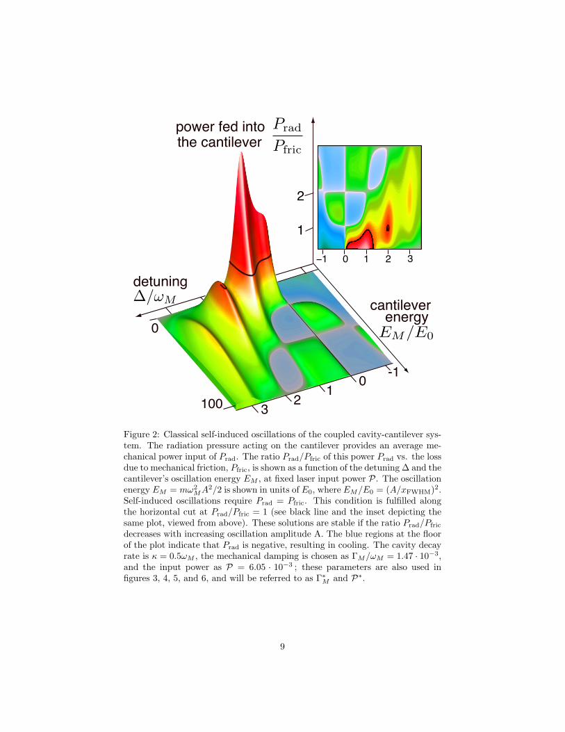
For each value of the oscillation amplitude A we can now plot the ratio betweenradiation power input and friction loss, Prad/Pfric = 〈Fradx〉/(ΓM 〈x2〉), aftereliminating x using Eq. 8. This is shown in Fig. 2. Power balance is fulfilled ifthis ratio is one, corresponding to the contour line Prad/Pfric = 1. If the powerinput into the cantilever by radiation pressure is larger than frictional losses(i.e., for a ratio larger than one), the amplitude of oscillations will increase,otherwise it will decrease. Stable solutions (dynamical attractors) are thereforegiven by that part of the contour line where the ratio decreases with increasingoscillation amplitude (energy), as shown in Fig. 2.

Changing the (dimensionless) mechanical damping rate ΓM/ωM will scalethe plot in Fig. 2 along the vertical axis, so that the horizontal cut at one yields adifferent contour line of stable solutions [a changed input power P gives a similarscaling, but leads to further changes in the solution, as P also enters the forcebalance condition, Eq. (8)]. Decreasing mechanical damping or increasing the

7

power input will increase the plot height in Fig. 2, so that the amplitude/energyof oscillation of the stable solution increases.

While the surface or contour plots in Fig. 2 allow a discussion of generalfeatures of the self-induced oscillations, such as the multistabilities discussedin Ref. [17], a slightly different representation of the classical solution is moreamenable to an easier understanding of the particular dynamics of the systemfor a certain set of fixed system parameters. Figure 3 shows the cantilever energyEM,cl = 1

2mω2MA

2 in terms of the classical energy scale E0 = 12mω

2Mx

2FWHM as

function of driving P and detuning ∆/ωM . These are the parameters that cantypically be varied in a given experimental setup.

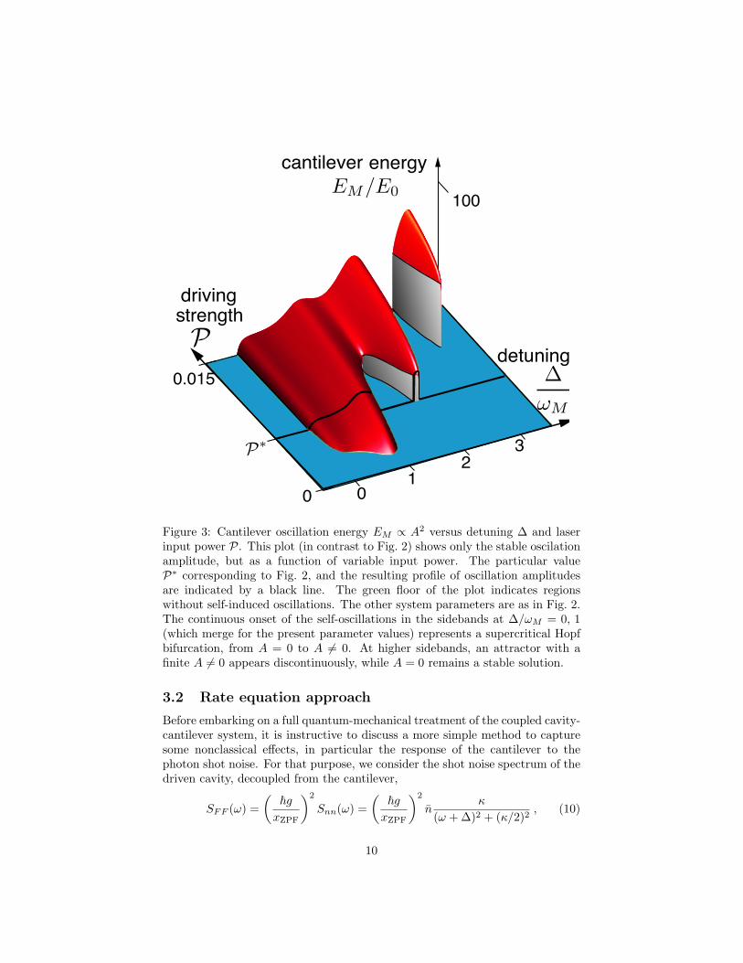
For sufficiently strong driving, self-induced oscillations appear around integermultiples of the cantilever frequency, ∆ ≈ nωM . For a cavity decay rate κ =0.5ωM assumed in Fig. 3, the different bands are distinguishable at lower driving;for larger κ (or for stronger driving), the various ‘sidebands’ merge. For thelower-order sidebands, the nonzero amplitude solution connects continuously tothe zero amplitude solution, which becomes unstable. This is an example of a(supercritical) Hopf bifurcation into a limit cycle.

The vertical faces, shown gray in Fig. 3, for ∆ ≈ 2ωM and ∆ ≈ 3ωM areconnected to the sudden appearance of attractors with a finite amplitude. Forexample, while approaching the detuning of ∆ = 2ωM at fixed P (the solidline in Fig. 3 refers to P = 1.47 · 10−3), a finite amplitude solution appears,although A = 0 remains stable. In Ref. [17] the existence of higher-amplitudestable attractors and, correspondingly, dynamic multistability were discussed.

8

detuning

01

23

0cantilever

energy

-1

100

power fed intothe cantilever

1

2

0 1 2 3

Figure 2: Classical self-induced oscillations of the coupled cavity-cantilever sys-tem. The radiation pressure acting on the cantilever provides an average me-chanical power input of Prad. The ratio Prad/Pfric of this power Prad vs. the lossdue to mechanical friction, Pfric, is shown as a function of the detuning ∆ and thecantilever’s oscillation energy EM , at fixed laser input power P. The oscillationenergy EM = mω2

MA2/2 is shown in units of E0, where EM/E0 = (A/xFWHM)2.

Self-induced oscillations require Prad = Pfric. This condition is fulfilled alongthe horizontal cut at Prad/Pfric = 1 (see black line and the inset depicting thesame plot, viewed from above). These solutions are stable if the ratio Prad/Pfric

decreases with increasing oscillation amplitude A. The blue regions at the floorof the plot indicate that Prad is negative, resulting in cooling. The cavity decayrate is κ = 0.5ωM , the mechanical damping is chosen as ΓM/ωM = 1.47 · 10−3,and the input power as P = 6.05 · 10−3 ; these parameters are also used infigures 3, 4, 5, and 6, and will be referred to as Γ∗M and P∗.

9

energy

0

detuning

driving

cantilever

12

3

0

0.015

100

strength

Figure 3: Cantilever oscillation energy EM ∝ A2 versus detuning ∆ and laserinput power P. This plot (in contrast to Fig. 2) shows only the stable oscilationamplitude, but as a function of variable input power. The particular valueP∗ corresponding to Fig. 2, and the resulting profile of oscillation amplitudesare indicated by a black line. The green floor of the plot indicates regionswithout self-induced oscillations. The other system parameters are as in Fig. 2.The continuous onset of the self-oscillations in the sidebands at ∆/ωM = 0, 1(which merge for the present parameter values) represents a supercritical Hopfbifurcation, from A = 0 to A 6= 0. At higher sidebands, an attractor with afinite A 6= 0 appears discontinuously, while A = 0 remains a stable solution.

3.2 Rate equation approach

Before embarking on a full quantum-mechanical treatment of the coupled cavity-cantilever system, it is instructive to discuss a more simple method to capturesome nonclassical effects, in particular the response of the cantilever to thephoton shot noise. For that purpose, we consider the shot noise spectrum of thedriven cavity, decoupled from the cantilever,

SFF (ω) =(

~gxZPF

)2

Snn(ω) =(

~gxZPF

)2

nκ

(ω + ∆)2 + (κ/2)2, (10)

10

where

n =P

8ζ2

(ωM/κ)2

(∆/ωM )2 + (κ/2ωM )2(11)

is the mean number of photons in the cavity. The maximum occupation nmax =Pω4

M/(2κ4ζ2) = 4α2

L/κ2 occurs at zero detuning. We note that in using the

unperturbed, intrinsic shot noise spectrum for an optical cavity in the absenceof optomechanical effects, we neglect the modification of that spectrum due tothe backaction of the cantilever motion.

The asymmetry of the shot noise spectrum is important for the dynamics ofthe cantilever. The spectral density of the radiation-pressure force at positivefrequency ωM (negative frequency −ωM ) yields the probability of the cavityabsorbing a phonon from (emitting a phonon into) the cantilever [12].

For a red-detuned laser impinging on the cavity (∆ < 0), the cavity’s noisespectrum peaks at positive frequencies and the cavity tends to rather absorbenergy from the cantilever. As a consequence, the mechanical damping rate forthe cantilever is increased, leading to cooling if one starts with a sufficientlyhot cantilever. In the opposite Raman-like process taking place at ∆ > 0,a blue-detuned laser beam will preferentially lose energy to the cantilever, sothat it matches the cavity’s resonance frequency. The effective optomechanicaldamping rate,

Γopt = ζ2κ2[Snn(+ωM )− Snn(−ωM )] , (12)

is then negative. The corresponding heating of the mechanical cantilever iscounteracted by the mechanical damping ΓM . Simple rate equations for theoccupancy of the cantilever yield a thermal distribution for the cantilever phononoccupation number nM , with [12]

〈c†c〉 = 〈nM 〉 =ζ2κ2Snn(−ωM ) + nthΓM

Γopt + ΓM. (13)

The effective temperature, Teff, is related by 〈nM+1〉/〈nM 〉 = exp[~ωM/(kBTeff)]to the mean occupation number. The equilibrium mechanical mode occupationnumber, nth, is determined by the mechanical bath temperature, which is takenas zero in the following. In contrast to first appearance, the mean occupationnumber of the cantilever given in Eq. (13) does not depend on the quantumparameter ζ, as ζ2Snn is independent of ζ. This is because Snn ∼ n ∼ 1/ζ2,see Eq. (11). The cantilever energy, therefore, only trivially depends on thequantum parameter as EM/E0 = 4ζ2 〈nM 〉, so that it vanishes in the classicallimit, where ζ2 ∝ ~→ 0.

In general, the phonon number in Eq. (13) can increase due to two distinctphysical effects: On the one hand, the numerator can become larger, due to theinfluence of photon shot noise impinging on the cantilever, represented by Snn.On the other hand, the denominator can become smaller due to Γopt becomingnegative. In the latter case, the fluctuations acting on the cantilever (boththermal and shot noise) are amplified. This effect is particularly pronouncedjust below the threshold of instability, where ΓM + Γopt = 0 (see below).

11

In the resolved sideband limit κ � ωM (at weak driving) the cantileveroccupation 〈nM 〉 will peak around zero detuning, where the number of photonsin the cavity is large, and around a detuning of ∆ = ωM . At the latter value ofdetuning the aforementioned Raman process is maximally efficient as a photonentering the cavity will exactly match the resonance frequency after excitinga phonon in the cantilever. This dependence of cantilever occupation (or thecorresponding energy) on the detuning is shown in Fig. 4.

The approach sketched above can be modified slightly to take account of themodification of the cavity length due to a static shift of the cantilever mirrorby radiation pressure. Approaching the resonance of the cavity from below, theincreasing number of photons inside the cavity will increase the cavity length dueto their radiation pressure on the mirror, bringing the system even closer to theresonance. The effect of the static shift of the mirror on the mean occupationof the cavity can be included self-consistently, leading to the tilt of the peakaround the resonance, shown by the dash-dotted line in Fig. 4(a). The samefigure also includes results of the full quantum mechanical approach, which willbe discussed in the next section.

For larger κ, the two peaks in the cantilever excitation merge. Higher-ordersidebands are not resolved within this approach, since they would require takingcare of the modification of SFF due to the cantilever’s motion.

Classical self-induced oscillations occur in a regime of larger driving, wherethe optomechanical damping rate Γopt of Eq. (12) becomes negative. Theyappear once amplification exceeds intrinsic damping, i.e. when Γopt + ΓM < 0.The simple rate equation approach lacks any feedback mechanism to stop thedivergence of the phonon number. The classical solution demonstrates how thisfeedback (i.e. the resulting change in the dynamics of the radiation field) makesthe mechanical oscillation amplitude saturate at a finite level. In addition, itshows the onset of self-induced oscillations to occur at a smaller detuning, dueto the effective shift of the cantilever position explained above.

12

rate equation

full master equationrate eqn. with correction

a b rate equationclassical curvefull master equationregion of instability

cfull master equationLangevin equation

cant

ileve

r ene

rgy

detuning

cant

ileve

r ene

rgy

detuning

cant

ileve

r ene

rgy

detuningd

classical curvefull master

Langevinequation

equation

detuning

cant

ileve

r ene

rgy

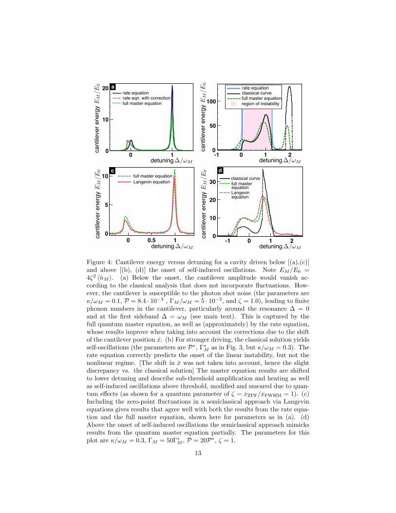
Figure 4: Cantilever energy versus detuning for a cavity driven below [(a),(c)]and above [(b), (d)] the onset of self-induced oscillations. Note EM/E0 =4ζ2 〈nM 〉. (a) Below the onset, the cantilever amplitude would vanish ac-cording to the classical analysis that does not incorporate fluctuations. How-ever, the cantilever is susceptible to the photon shot noise (the parameters areκ/ωM = 0.1, P = 8.4 · 10−3 , ΓM/ωM = 5 · 10−3, and ζ = 1.0), leading to finitephonon numbers in the cantilever, particularly around the resonance ∆ = 0and at the first sideband ∆ = ωM (see main text). This is captured by thefull quantum master equation, as well as (approximately) by the rate equation,whose results improve when taking into account the corrections due to the shiftof the cantilever position x. (b) For stronger driving, the classical solution yieldsself-oscillations (the parameters are P∗, Γ∗M as in Fig. 3, but κ/ωM = 0.3). Therate equation correctly predicts the onset of the linear instability, but not thenonlinear regime. [The shift in x was not taken into account, hence the slightdiscrepancy vs. the classical solution] The master equation results are shiftedto lower detuning and describe sub-threshold amplification and heating as wellas self-induced oscillations above threshold, modified and smeared due to quan-tum effects (as shown for a quantum parameter of ζ = xZPF/xFWHM = 1). (c)Including the zero-point fluctuations in a semiclassical approach via Langevinequations gives results that agree well with both the results from the rate equa-tion and the full master equation, shown here for parameters as in (a). (d)Above the onset of self-induced oscillations the semiclassical approach mimicksresults from the quantum master equation partially. The parameters for thisplot are κ/ωM = 0.3, ΓM = 50Γ∗M , P = 20P∗, ζ = 1.

13

In Fig. 4(b) we show results for the detuning dependence of the mean energyof the cantilever obtained from this rate equation approach below the thresh-old of classical self-induced oscillations. The coupled cavity-cantilever systemacts as an amplifier of fluctuations, increasing the occupation of higher numberstates of the cantilever well before classical oscillations set in. At the onsetof classical self-induced oscillations the rate equation result diverges. A fullquantum-mechanical treatment describes the crossover of the cantilever dynam-ics from quantum-fluctuation induced heating to self-induced oscillations as willbe discussed now.

3.3 Quantum master equation method

The evolution of the coupled quantum system comprised of the cantilever andthe optical cavity is described by the Hamiltonian of Eq. (3). Dissipation arisesfrom the coupling of the mechanical mode to a bath and due to the openingof the cavity to the outside. While the former results in mechanical dampingwith a rate ΓM , the latter is associated with the ringdown rate of the cavityκ. In the present paper, we will assume the mechanical bath to be at zerotemperature, where quantum effects are most pronounced in steady state. Afuture, more realistic treatment, should relax this assumption and deal with thenonequilibrium dynamics that results when a mechanical system is first cooledoptomechanically and then switched to the unstable side.

The system can be described by a reduced density matrix ρ for the mechan-ical cantilever mode and the optical mode of the cavity. In the frame rotatingat the laser frequency, the time evolution of the density matrix ρ is given by

d

dtρ =

[H0, ρ]i~

+ ΓM D[c] + κD[a] , (T ≡ 0) (14)

where D[A] = AρA† − 12 A†Aρ − 1

2 ρA†A denotes the standard Lindblad opera-

tor. The Hamilton operator H0 describes the coherent part of the evolution ofthe coupled cavity-cantilever system,

H = H0 + Hκ + HΓ .

For the numerical evaluation, we rewrite Eq. 14 as dρ/dt = Lρ, with a Liouvilliansuperoperator L. We then interpret the density matrix as a vector, whose timeevolution is governed by the matrix L. The density matrix at long times (insteady state) is then given by the eigenvector of L with eigenvalue 0. Thenumerical calculation of this eigenvector is much more efficient than a simulationof the full time evolution. Since we are dealing with large sparse matrices, itis convenient to employ an Arnoldi method that finds a few eigenvalues andeigenvectors of L by iterative projection. For Hermitean matrices, the Arnoldimethod is also known as the Lanczos algorithm.

In practice, the numerical approach used here sets strong limits on the di-mension of the Hilbert space. We need to take into account the Na lowest Fockstates of the cavity and the Nc lowest Fock states of the mechanical cantilever,

14

resulting in a Liouvillian superoperator with (Na × Nc)4 elements. This putsmore severe restrictions on our treatment of the coupled cavity-cantilver systemthan encountered in similar treatments of comparable systems. For example,nanoelectromechanical systems, where an oscillator is coupled to a normal-stateor superconducting single-electron transistor (SET), will have to account foronly a very limited number of charge states of the SET (namely those few in-volved in the relevant transport cycle). As a consequence, a larger number ofFock states can be included, e.g., 70 number states of the oscillator were kept inRef. [28]. In some cases it was furthermore considered sufficient to treat onlythe incoherent dynamics of the mechanical oscillator, i.e., only the elements ofthe density matrix diagonal in the oscillator’s Fock space, thereby reaching 200number states of a mechanical mode coupled to a normal-state SET [41]. Therestricted number of Fock states that can be considered here makes it more dif-ficult to fully bridge the gulf to the classical regime of motion of the mechanicalcantilever. [(Na, Nc) = (8,16) for Fig. 4(a),(c),(d), (4,22) for Figs. 4(b), 5 andfor the first two panels of 6, (3,35) for the last panel of Fig. 6]

A first comparison of results of the quantum master equation to the classicalsolution and the results of the rate equation was already shown in Fig. 4. We findthat the full quantum results do not qualitatively differ from the rate equationresults provided the parameters are chosen sufficiently far from the onset of self-induced oscillations. However, only the quantum master equation approach isable to describe the crossover from sub-threshold quantum fluctuations (whereEM ∝ ζ2) to the large classical cantilever energies associated with self-inducedoscillations.

In Fig. 5 we demonstrate the influence of the quantum parameter ζ =xZPF/xFWHM governing the crossover between the classical and the quantumregime.

Figure 5(a) shows the cavity photon number, normalized to its value at res-onance, nmax. For our choice of driving parameter P, the maximal occupationnmax is low, so that a small number of Fock states suffices for describing the cav-ity in the quantum master equation. This allows to account for enough numberstates of the cantilever to reach the regime of self-induced oscillations. The clas-sical solution (solid black line) consists of the broad Lorentzian of the isolatedcavity, on top of which additional peaks appear. These are due to the classicalself-induced oscillations occuring at the sidebands ∆ = ωM , 2ωM , . . . in the cou-pled cavity-cantilever system. Figure 5(c) displays the cantilever energy EM/E0

as a function of the detuning, ∆/ωM , with features that parallel those foundfor the photon number. The classical curve in (b), shown in black, correspondsto the cut indicated by the solid line in Fig. 3. For the chosen driving power,the second sideband at ∆ = ωM just starts to appear, while the first sidebandis merged with the resonance at ∆ = 0, which shows up as a slight shoulder.The sharpness and strength of these features also depend on the values of me-chanical damping and cavity decay rate. Results of our solution of the quantummaster equation are shown for three different values of the quantum parameterζ = xZPF/xFWHM. Due to restrictions of the numerical resources, it was notfeasible to map out a wider range of values of the parameter ζ, although the

15

range analysed here already suffices to describe the quantum-classical crossover.The quantum master equation shows results that are qualitatively similar to

the classical solution in the regime of self-induced oscillations, with the peaksbeing progressively broadened, reduced in height, and shifted to lower detuningfor increasing values of the quantum parameter ζ. Numerical evidence indicatesthat quantum correlations between the cantilever position operator x and thephoton operators a†, a may cause the observed shift. As expected, the dis-crepancy between the quantum mechanical and the classical result reduces withdiminishing quantum parameter ζ. In Fig. 5(b), we show the dependence ofthe cantilever energy on the quantum parameter, for two different values of thedetuning. In the sub-threshold regime of amplification/heating the cantileverenergy scales as ζ2, as discussed above. In any case, the classical limit is clearlyreached as ζ → 0.

At the second sideband a classical solution of finite amplitude coexists witha stable zero-amplitude solution (compare Fig. 2 and last panel of Fig. 6). Theblack curve in Fig. 5(b), showing the finite amplitude solution, may thereforedeviate substantially from the ~ → 0 limit of the quantum mechanical result.In general, the average value of EM , shown here, will be determined by therelative weight of the two solutions (which are connected by tunneling due tofluctuations), as well as fluctuations of EM for each of those two attractors.

3.4 Langevin equation

To get an estimate of the influence of quantum fluctuations, we compare theresults of the quantum master equation to numerical simulations of classicalLangevin equations that try to mimick the quantum noise. The resulting de-scription of the quantum-to-semiclassical crossover is illustrated in Figs. 4(c).To imitate both the zero-point fluctuations of the mechanical oscillator and theshot-noise inside the cavity, we add white noise terms to Eqs.4and 5:

α = [i(∆ + gx

xZPF)− κ

2]α− iαL +

√κ/2αin (15)

x = −ω2Mx+

~gmxZPF

|α|2 − ΓM x+√

~ωMΓ/mξ, (16)

where 〈αin〉 = 〈ξ〉 = 0 and 〈αin(t)α∗in(t′)〉 = 〈ξ(t)ξ(t′)〉 = δ(t − t′). The co-efficients in front of the noise terms are chosen such that in the absence ofoptomechanical coupling we obtain the zero-point fluctuations, i.e.

⟨|α|2

⟩= 0.5

away from resonance and mω2M

2 〈x2〉 = ~ωM

4 . The mean zero-point energy of thecantilever is substracted from the curve in Fig.4(c).

For parameters below the onset of self-sustained oscillations, this semiclassi-cal approach leads to good qualitative agreement with the quantum mechanicaldescription, as can be seen in Fig. 4(c) for parameters that are the same asthose of 4(a). Still, the Langevin approach can mimick the results from themaster equation only partially. In particular, the approximation gets worse

16

when dealing with low photon numbers. This is because the Langevin equationintroduces artificial fluctuations of the radiation pressure force in the vacuumstate. Indeed, |α|2 has a finite variance even in the ground state of the photonfield, in contrast to a†a.

3.5 Wigner density and phonon number distribution

In figure 6, we go beyond the average cantilever phonon number and presentresults both for the phonon number probability distribution, as well as the fullWigner density of the cantilever, defined as

W (x, p) =1π~

∫ +∞

−∞〈x− y |ρ|x+ y〉 e2ipy/~ dy. (17)

This figure demonstrates the different nature of the cantilever dynamics inthe sub-threshold regime and above threshold, where self-induced oscillations oc-cur. Below the threshold (for a detuning ∆a = −0.45ωM as indicated in Fig. 5,quantum parameter ζ = 1, and other parameters as in Fig. 5) the occupation ofthe cantilever is thermal, with an effective temperature determined by the effec-tive optomechanical and mechanical damping rates, cf. Eq. (13). Consequently,the Wigner density shows a broad peak around the origin of the x− p plane ofcantilever position and momentum (the static shift of the cantilever due to theradiation pressure is very small). For a detuning of ∆b = −0.2ωM , self-inducedoscillations occur. The probability distribution for the phonon number showssome thermal broadening, but an additional peak appears at a finite phononnumber. In the Wigner density plot this results in a crater-like feature, whichcorresponds to a mixture of coherent states with essentially fixed amplitudebut arbitrary phases. This captures the fact that the phase of the self-inducedoscillations is completely arbitrary also in the classical solution. The energycorresponding to the phonon number at which the distribution peaks, comparesfairly well to the oscillation energy obtained from the classical solution. Onlythe shift towards lower values of detuning as shown in Fig. 5(b) puts restrictionson a detailed quantitative comparison.

17

quantum parameterphot

on n

umbe

r

= 1.3

= 0.7 = 1.0

classical curve

detuning

= 1.3

= 0.7 = 1.0

classical curve

cant

ileve

r ene

rgy

detuning

classicalquantum

cant

ileve

r ene

rgy

detuning

Fano

fact

or

a b

c d

Figure 5: Comparison of classical and quantum results. (a) Number of photonsinside the cavity as a function of detuning, and (c) energy of the cantilever versusdetuning for Γ∗M , P∗ and κ/ωM = 0.5. The dotted curves show results fromthe quantum master equation for different values of the quantum parameterζ = 1.3 (pink) , ζ = 1.0 (green) and ζ = 0.7 (blue), which are comparedwith the solution of the classical equations of motion (black solid curve). Asζ → 0, the qantum result approaches the classical curve. See main text fora detailed discussion. (b) The energy of the cantilever as a function of thequantum parameter ζ for fixed detunings ∆b/ωM = −0.2 and ∆c/ωM = 0.4(the detuning value ∆a indicated in (b) is used in Fig. 6). (d) Fano factor(〈n2

M 〉 − 〈nM 〉2)/〈nM 〉 vs. detuning, for ζ = 1. For a coherent state whoseoccupation number follows a Poisson distribution, the Fano factor is 1 (dashedblack line). Close to the resonance (and far away from it, where 〈nM 〉 = 0),the results of the quantum master equation approach this value. The Fanofactor becomes particularly large near the second sideband, where we observecoexistence of different oscillation amplitudes (see Fig. 6).

18

0.08

-5

5

0

-5 0

0.03

10

-10

010

-100-5

0.15

0

5

-5

50 5

Wignerdensity

prob

abilit

y

phonon number

prob

abilit

y

phonon number

prob

abilit

y

phonon number

Figure 6: Distribution functions P (nM ) of the cantilever occupation and Wignerfunctions W (x, p) [rescaled by xZPFpZPF] of the cantilever for ∆a = −0.45ωM ,∆b = −0.2ωM , ∆d = 1.72ωM [corresponding to the detuning values also indi-cated in Fig. 5(b); further parameters as in Fig. 5 with ζ = 1.0; for ∆d themechanical damping rate is reduced to ΓM/ωM = 1.2 · 10−3]. Below the thresh-old of self-induced oscillations, a broadened distribution is found correspondingto an increased effective temperature, cf. Eq. (13) (left panels, ∆a); self-inducedoscillations are visible as a finite amplitude ring in the middle and the rightpanel. Dynamical multistability (i.e. co-existence of several attractors) in theclassical solution becomes apparent both in the distribution and the Wignerdensity, where a double-peaked structure develops.

For a value of the detuning located in the second sideband, ∆d = 1.72ωM , wefind a probability distribution with a peak for the occupation of the cantileverground state, and a broader peak at a finite occupation number (mechanicaldamping is slightly decreased to display more pronounced features). Likewise,the Wigner density consists of a sharp peak at the origin, surrounded by abroader ring representing finite amplitude oscillations. This corresponds tothe existence of two stable attractors in the classical analysis, with vanishingand finite oscillation amplitude, respectively. Similar results for the Wignerdensities were found in Ref. [28] for a cantilever driven by a superconductingsingle-electron transistor.

4 Conclusion

We presented a fully quantum mechanical treatment of a driven optical cavitycoupled to a mechanical cantilever by radiation pressure. Light-induced forcescan yield a negative contribution to the damping of the cantilever, causing

19

amplification of fluctuations and even instabilities of the cantilever dynamics.In the present paper we first reviewed briefly the classical solution and dis-

cussed the existence of self-induced oscillations and the resulting attractor di-agram of the system. We paid particular attention to the resolved-sidebandregime κ � ωM , which is now increasingly studied in experimental setups.Here the instabilities clearly occur at sidebands, where the detuning matchesan integer multiple of the mechanical frequency.

Within a simple rate equation approach, we were able to discuss the influ-ence of the photon shot noise and quantum fluctuations well below the instabilitythreshold. The full quantum-mechanical treatment, based on a numerical solu-tion of the quantum master equation, is able to completely describe both regimes(below and above threshold). It has been complemented by numerical studies ofa Langevin equation that includes the zero-point fluctuations in a semiclassicalway. We studied the crossover between the quantum and classical regime, whichis governed by the quantum parameter, ζ = xZPF/xFWHM , denoting the ratiobetween the mechanical zero-point fluctuation amplitude and the width of theoptical resonance. Signatures of the self-induced oscillations are also found inthe full quantum mechanical solution, even at larger values of ζ. In regions ofdynamical multistability, the different attractors show up simultaneously in thesteady state of the cantilever, since the quantum noise can induce transitionsbetween those attractors. Finally, we characterized the mechanical motion inthe various regimes by discussing the phonon number probability distributionas well as the Wigner density.

Acknowledgments

We thank A. Clerk, S. Girvin, K. Karrai, C. Neuenhahn, C. Metzger, I. Favero,D. Rodrigues, and J. Harris for discussions and fruitful collaboration on theoptomechanical instability. We acknowledge support by the DFG, in the formof the Nanosystems Initiative Munich (NIM), the SFB 631, and the Emmy-Noether program.

References

[1] V.B. Braginsky and A.B. Manukin. Ponderomotive effects of electromag-netic radiation. Soviet Physics JETP, 25:653, 1967.

[2] V. B. Braginsky, A. B. Manukin, and M. Yu. Tikhonov. Investigationof dissipative ponderomotove effects of electromagnetic radiation. SovietPhysics JETP, 31:829, 1970.

[3] A. Dorsel, J. D. McCullen, P. Meystre, E. Vignes, and H. Walther. Opticalbistability and mirror confinement induced by radiation pressure. Phys.Rev. Lett., 51:1550, 1983.

20

[4] P. F. Cohadon, A. Heidmann, and M. Pinard. Cooling of a mirror byradiation pressure. Phys. Rev. Lett., 83:3174, 1999.

[5] C. Hohberger-Metzger and K. Karrai. Cavity cooling of a microlever. Na-ture, 432:1002, 2004.

[6] O. Arcizet, P. F. Cohadon, T. Briant, M. Pinard, and A. Heidmann.Radiation-pressure cooling and optomechanical instability of a micro-mirror. Nature, 444:71, 2006.

[7] S. Gigan et al. Self-cooling of a micromirror by radiation pressure. Nature,444:67, 2006.

[8] A. Schliesser, P. Del’Haye, N. Nooshi, K. J. Vahala, and T. J. Kippenberg.Cooling of a micro-mechanical oscillator using radiation pressure induceddynamical back-action. Phys. Rev. Lett., 97:243905, 2006.

[9] D. Kleckner and D. Bouwmeester. Sub-kelvin optical cooling of a microme-chanical resonator. Nature, 444:75, 2006.

[10] T. Corbitt et al. Toward achieving the quantum ground state of a gram-scale mirror oscillator. Phys. Rev. Lett., 98:150802, 2007.

[11] J. D. Thompson, B. M. Zwickl, A. M. Jayich, F. Marquardt, S. M. Girvin,and J. G. E. Harris. Strong dispersive coupling of a high finesse cavity toa michromechanical membrane. arXiv:0707.1724, 2007.

[12] F. Marquardt, J. P. Chen, A. A. Clerk, and S. M. Girvin. Quantum theoryof cavity-assisted sideband cooling of mechanical motion. Phys. Rev. Lett.,99:093902, 2007.

[13] I. Wilson-Rae, N. Nooshi, W. Zwerger, and T. J. Kippenberg. Theory ofground state cooling of a mechanical oscillator using dynamical back-action.Phys. Rev. Lett., 99:093901, 2007.

[14] J. M. Aguirregabiria and L. Bel. Delay-induced instability in a pendularFabry-Perot cavity. Phys. Rev. A, 36:3768, 1987.

[15] C. Fabre, M. Pinard, S. Bourzeix, A. Heidmann, E. Giacobino, and S. Rey-naud. Quantum-noise reduction using a cavity with a movable mirror.Phys. Rev. A, 49:1337, 1994.

[16] V. B. Braginsky, S. E. Strigin, and S. P. Vyatchanin. Parametric oscillatoryinstability in Fabry-Perot interferometer. Physics Letters A, 287:331, 2001.

[17] F. Marquardt, J. G. E. Harris, and S. M. Girvin. Dynamical multistabil-ity induced by radiation pressure in high-finesse micromechanical opticalcavities. Phys. Rev. Lett., 96:103901, 2006.

21

[18] C. Hohberger and K. Karrai. Self-oscillation of micromechanical resonators.Nanotechnology 2004, Proceedings of the 4th IEEE conference on nanotech-nology, page 419, 2004.

[19] T. Carmon, H. Rokhsari, L. Yang, T. J. Kippenberg, and K. J. Vahala.Temporal behavior of radiation-pressure-induced vibrations of an opticalmicrocavity phonon mode. Phys. Rev. Lett., 94:223902, 2005.

[20] T. J. Kippenberg, H. Rokhsari, T. Carmon, A. Scherer, and K. J. Vahala.Analysis of radiation-pressure induced mechanical oscillation of an opticalmicrocavity. Phys. Rev. Lett., 95:033901, 2005.

[21] M. Ludwig, C. Neuenhahn, C. Metzger, A. Ortlieb, I. Favero, K. Karrai,and F. Marquardt. Self-induced oscillations in an optomechanical system.arXiv:0711.2661, 2007.

[22] K. R. Brown, J. Britton, R. J. Epstein, J. Chiaverini, D. Leibfried, andD. J. Wineland. Passive cooling of a micromechanical oscillator with aresonant electric circuit. Phys. Rev. Lett., 99:137205, 2007.

[23] Ya. M. Blanter, O. Usmani, and Yu. V. Nazarov. Single-electron tunnelingwith strong mechanical feedback. Phys. Rev. Lett., 93(13):136802, Sep2004.

[24] A. A. Clerk and S. Bennett. Quantum nanoelectromechanics with electrons,quasi-particles and Cooper pairs: effective bath descriptions and strongfeedback effects. New Journal of Physics, 7:238, 2005.

[25] M. P. Blencowe, J. Imbers, and A. D. Armour. Dynamics of a nanome-chanical resonator coupled to a superconducting single-electron transistor.New Journal of Physics, 7:236, 2005.

[26] A. Naik et al. Cooling a nanomechanical resonator with quantum back-action. Nature, 443:193, 2006.

[27] S. D. Bennett and A. A. Clerk. Laser-like instabilities in quantum nano-electromechanical systems. Phys. Rev. B, 74:201301, 2006.

[28] D. A. Rodrigues, J. Imbers, and A. D. Armour. Quantum dynamics of aresonator driven by a superconducting single-electron transistor: a solid-state analogue of the micromaser. Phys. Rev. Lett., 98:067204, 2007.

[29] D. A. Rodrigues, J. Imbers, T. J. Harvey, and A. D. Armour. Dynami-cal instabilities of a resonator driven by a superconducting single-electrontransistor. New Journal of Physics, 9:84, 2007.

[30] C. A. Regal, J. D. Teufel, and K. W. Lehnert. Measuring nanomechanicalmotion with a microwave cavity interferometer, 2008.

[31] D. Meiser and P. Meystre. Coupled dynamics of atoms and radiation-pressure-driven interferometers. Phys. Rev. A, 73:033417, 2006.

22

[32] K. W. Murch, K. L. Moore, S. Gupta, and D. M. Stamper-Kurn. Mea-surement of Intracavity Quantum Fluctuations of Light Using an AtomicFluctuation Bolometer. arXiv:0706.1005v2, 2007.

[33] S. Bose, K. Jacobs, and P. L. Knight. Scheme to probe the decoherence ofa macroscopic object. Phys. Rev. A, 59:3204, 1999.

[34] W. Marshall, C. Simon, R. Penrose, and D. Bouwmeester. Towards quan-tum superpositions of a mirror. Physical Review Letters, 91(13):130401,2003.

[35] M. Pinard, A. Dantan, D. Vitali, O. Arcizet, T. Briant, and A. Heidmann.Entangling movable mirrors in a double-cavity system. Europhysics Letters,72:747, 2005.

[36] E. Buks, E. Segev, S. Zaitsev, B. Abdo, and M. P. Blencowe. Quantumnondemolition measurement of discrete fock states of a nanomechanicalresonator. EPL (Europhysics Letters), 81(1):10001 (5pp), 2008.

[37] T. J. Kippenberg and K. J. Vahala. Cavity opto-mechanics. Optics Express,15:17172, 2007.

[38] F. Marquardt, A. A. Clerk, and S. M. Girvin. Quantum theory of optome-chanical cooling. arXiv:0803.1164 (to be submitted to the proceedings of the”Physics of Quantum Electronics 2008” conference), 2008.

[39] O. Usmani, Ya. M. Blanter, and Yu. V. Nazarov. Strong feedback andcurrent noise in nanoelectromechanical systems. Physical Review B (Con-densed Matter and Materials Physics), 75(19):195312, 2007.

[40] A. Schliesser, R. Riviere, G. Anetsberger, O. Arcizet, and T. J. Kip-penberg. Resolved sideband cooling of a micromechanical oscillator.arXiv:0709.4036, 2007.

[41] M. Merlo, F. Haupt, F. Cavaliere, and M. Sassetti. Sub-poissonian phononicpopulation in a nanoelectromechanical system. New Journal of Physics,10(2):023008 (12pp), 2008.

23