MATH 220: 3.11 page 1 http://kunklet.people.cofc.edu/ Jan 3, 2021 3.11: The Hyperbolic Trig Functions Definition 3.11.1. The hyperbolic sine and cosine of x are cosh x = e x + e −x 2 sinh x = e x − e −x 2 The other four hyperbolic trig functions are defined in terms of these: tanh x = sinh x cosh x coth x = cosh x sinh x sech x = 1 cosh x csch x = 1 sinh x Similarities of the hyperbolic trig functions to the circular trig functions 1. cosh 0 = 1 sinh 0 = 0 2. cosh x is an even function. sinh x is an odd function. 3. cosh 2 x − sinh 2 x =1 4. cosh x cosh y + sinh x sinh y = cosh(x + y ) sinh x cosh y + cosh x sinh y = sinh(x + y ) 5. f (x) f ′ (x) sinh x cosh x cosh x sinh x tanh x sech 2 x coth x − csch 2 x sech x − sech x tanh x csch x − csch x coth x f (x) f ′ (x) sin x cos x cos x − sin x tan x sec 2 x cot x − csc 2 x sec x sec x tan x csc x − csc x cot x
Transcript
MATH 220: 3.11 page 1http://kunklet.people.cofc.edu/ Jan 3, 2021
3.11: The Hyperbolic Trig Functions
Definition 3.11.1. The hyperbolic sine and cosine of x are
cosh x =ex + e−x
2sinh x =
ex − e−x
2
The other four hyperbolic trig functions are defined in terms of these:
tanhx =sinhx
coshxcothx =
coshx
sinhxsech x =
1
coshxcsch x =
1
sinh x
Similarities of the hyperbolic trig functions to the circular trig functions
1. cosh 0 = 1 sinh 0 = 0
2. coshx is an even function. sinh x is an odd function.
3. cosh2 x− sinh2 x = 1
4. coshx cosh y + sinhx sinh y = cosh(x+ y)
sinh x cosh y + coshx sinh y = sinh(x+ y)
5.
f(x) f ′(x)
sinhx cosh x
coshx sinhx
tanhx sech2 x
cothx − csch2 x
sech x − sech x tanhx
csch x − csch x cothx
f(x) f ′(x)
sinx cosx
cosx − sinx
tanx sec2 x
cot x − csc2 x
secx secx tanx
cscx − cscx cotx
MATH 220: 3.11 page 2http://kunklet.people.cofc.edu/ Jan 3, 2021
Graphs of the hyperbolic trig functions
x
y = cosh x
x
y = sinh x
MATH 220: 3.11 page 3http://kunklet.people.cofc.edu/ Jan 3, 2021
Some limits involving the hyperbolic trig functions
3.11.e1. Evaluate the limits, if they exist.
a. limx→∞
coshx b. limx→−∞
coshx c. limx→∞
sinhx
d. limx→−∞
sinhx e. limx→∞
tanhx f. limx→∞
5ex − e−2x
3ex + 4e−2x
MATH 220: 6.1 page 4http://kunklet.people.cofc.edu/ July 16, 2020
Tip: It is far easier to remember the way to do problems in this chapter than the formula.
6.1: Areas Between Curves
6.1.e1. Find the area of the region bounded by the curves y = x2 and y = 2x.
6.1.e1, continued. Here’s another solution, obtained with a different way of slicing.
MATH 220: 6.1 page 5http://kunklet.people.cofc.edu/ July 16, 2020
6.1.e2. Find the area of the region bounded by y = x2 and y = (x− 2)2 and y = 0.What will be the easiest way to slice up this region?
MATH 220: 6.2 page 6http://kunklet.people.cofc.edu/ July 16, 2020
6.2: Volumes
Calculating volumes by slicing
6.2.e1. A (three-dimensional) solid has for its base the region in the xy-plane bounded byy = x2 and y = 2x. Find the volume of the solid if its cross-sections perpendicular to thex-axis are squares with one side in the plane.
Tip: To answer the question perfectly doesn’t require a great drawing. Usually, it onlyneeds to represent where one curve lies relative to the other(s).
MATH 220: 6.2 page 7http://kunklet.people.cofc.edu/ July 16, 2020
6.2.e2. The intersection of a solid with the xy-plane is the region bounded by y = x2 andy = 2x. Find the volume of the solid if its cross-sections perpendicular to the y-axis arecircles with diameters in the plane.
See more of this type of volume problem athttp://kunklet.people.cofc.edu/MATH220/stew0602prob.pdf
MATH 220: 6.2 page 8http://kunklet.people.cofc.edu/ July 16, 2020
Volumes of Revolution: the method of discs and washers
6.2.e3. The region bounded by y = x2 and y = 2x − x2 is rotated about the line y = 0.Find the volume swept out by the region.
MATH 220: 6.2 page 9http://kunklet.people.cofc.edu/ July 16, 2020
6.2.e4. The region bounded by y = x2 and y = 4 is rotated about the line y = 4. Findthe volume swept out by the region.
6.2.e5. The region bounded by y = x2 and y = 2x is rotated about the line x = 2. Findthe volume swept out by the region.
We’ll see another technique for solving 6.2.e5 in the next section.
MATH 220: 6.3 page 10http://kunklet.people.cofc.edu/ July 16, 2020
6.3: More Volumes
Volumes of Revolution: the method of cylindrical shells
Let’s apply this method to the last example in the previous section:
6.2.e5, continued. The region bounded by y = x2 and y = 2x is rotated about the line x = 2.Find the volume swept out by the region. Express your answer as a definite integral.
MATH 220: 6.3 page 11http://kunklet.people.cofc.edu/ July 16, 2020
Tip: Don’t ask “Should I use shells or washers?” Instead, ask “Is it easier to slice theregion vertically or horizontally?”
6.3.e1. Let R be the region in the plane bounded by y = x and y = 2 − x2. Find thevolume swept out as R is rotated about the line x = 4. Express your answer as a definiteintegral.
6.3.e1, continued. Find the volume swept out as R is rotated about y = 2. Express youranswer as a definite integral.
MATH 220: 6.3 page 12http://kunklet.people.cofc.edu/ July 16, 2020
6.3.e2. Let R be the triangle with vertices (−1, 2), (0, 1), and (3, 2).
a. Find the volume swept out by R when it is rotated about y = 2.
b. Find the volume swept out by R when it is rotated about x = 3.
c. Find the volume of the solid whose intersection with the plane is R and whose cross-sections perpendicular to the y-axis are squares with a side in the plane.
Express your answers as definite integrals.
MATH 220: 6.4 page 13http://kunklet.people.cofc.edu/ July 16, 2020
6.4: Work
When a constant force is applied to an object moving in a straight line in the same directionas the force, the work done by that force is, by definition, its magnitude times the distancetraveled by the object.Work can be measured in foot-pounds or Newton-meters (also known as Joules). Forinstance, if I lift a 2-pound calculus book 3 feet in the air, I’ve done 6 foot-pounds of work.
In this section, we’ll use integrals to find work in cases when the force is not constant.
6.4.e1. A rope 50 feet long hangs from the top of a tall tower. If the rope weighs 30 lbs,find the work to pull 40 ft of the rope to the top of the tower.
6.4.e2. Suppose a 10-lb weight is attached to the end of the rope in 6.4.e1. Find the workto pull the rope and weight to the top of the tower.
MATH 220: 6.4 page 14http://kunklet.people.cofc.edu/ July 16, 2020
6.4.e3. A one-pound bucket initially holds 50 pounds of sand, but as it is lifted, the sandleaks from the bucket at a rate of 2
3pounds per foot. Find the work to lift the leaky bucket
and its contents 75 feet.
MATH 220: 6.4 page 15http://kunklet.people.cofc.edu/ July 16, 2020
Spring problems
A spring has a natural resting length. To hold the spring at a length different from itsnatural length requires a force which has the following simple description.
Hooke’s Law. The force f(x) necessary to hold a spring x meters from its natural lengthis proportional to x. That is, for some spring constant k,
f(x) = kx
To stretch or compress a spring beyond its natural length requires work.
Tips: (1) In a spring-work problem, don’t confuse force, measured in pounds or Newtons,and work, measured in foot-pounds or Joules.
(2) Look for the information that will allow you to solve for the spring constant k.
6.4.e4. A 2-Newton force will hold a spring 0.1m from its resting length.
a. Find the work done in stretching the spring from 0m to 0.1m beyond its natural length.
b. Find the work needed to stretch the spring from 0.1m to 0.2m beyond its natural length.
MATH 220: 6.4 page 16http://kunklet.people.cofc.edu/ July 16, 2020
6.4.e5. The work to pull a spring from resting length to 10cm beyond that length is 2J.
a. Find the spring constant for this spring.
b. Find the work to pull the spring from 20cm to 30cm beyond its natural length.
c∗. Starting from its natural length, how far will 1J of work stretch the spring?
Tip: All work problems look alike in the following sense: If an object moves along an axisfrom x = a to x = b, and if the force applied to the object when at position x is f(x), then
dw = f(x) dx and w =
∫ b
a
f(x) dx
MATH 220: 6.5 page 17http://kunklet.people.cofc.edu/ July 17, 2020
6.5: Average Value
Definition 6.5.1. The average value of the function f(x) on the interval [a, b] is
fave =1
b− a
∫ b
a
f(x) dx
Since
(b− a)fave =
∫ b
a
f(x) dx,
fave is the altitude of the horizontal line that captures the same area as f over [a, b]:
x
y
x
y
y = f(x)
y = fave
∫ b
af(x) dx(b− a)fave =
a ab b
6.5.e1. The graphs below show the temperature T in downtown Charleston as a functionof time t over two different days. On both days, the high was 90◦ and the low was 50◦,but the second day had a higher average temperature. Can you see why?
t
T
0 24
50
90
Tave
t
T
0 24
50
90Tave
Note that the average value of a given function depends on the interval. In either of thegraphs above, the average temperature over the first 12 hours of the day is lower than theaverage over the last 12 hours, in the same way that the average of a your first 4 quizzesmight be different than the average of your last four quizzes.
MATH 220: 6.5 page 18http://kunklet.people.cofc.edu/ July 17, 2020
6.5.e2. Calculate the average of x2 on the interval [−1, 2]
x
y
1 2-1
1
2
3
4
6.5.e3. Calculate the average of the function graphed atright on the interval [0, 3].
x
y
1 2 3
1
Mean Value Theorem for Integrals 6.5.2. If f(x) is continuous on the interval [a, b],then there exists at least one number c in [a, b] for which f(c) = fave.
6.5.e3, continued. Find the number(s) c in [−1, 2] guaranteed by the MVTI 6.5.2 for thefunction x2.
One last note. When we calculate the average of an object’s velocity s′(t) over an intervalof time [a, b],
1
b− a
∫ b
a
s′(t) dt =s(b)− s(a)
b− a
we obtain the object’s change in position over the change in time. That is, “average veloc-ity” as defined in this section is the same as “average velocity” as defined in precalculus.
MATH 220: 7.1 page 19http://kunklet.people.cofc.edu/ July 18, 2020
7.1: Integration by Parts
If u and v are differentiable functions of x, then the derivative of their product is
d
dx(uv) = u
dv
dx+ v
du
dx
and so ∫ (
udv
dx+ v
du
dx
)
dx = uv.
Distribute the dx, write dudxdx = du and dv
dxdx = dv, and break the integral in two:
∫
u dv +
∫
v du = uv.
Finally, subtract the second integral from both sides and we obtain the formula known asIntegration by Parts:
∫
u dv = uv −∫
v du
IBP is sometimes useful in integrating a product:
7.1.e1. Integrate:∫xex dx
Sometimes we use IBP twice in the same problem:
7.1.e2. Integrate:∫x2 cosx dx
MATH 220: 7.1 page 20http://kunklet.people.cofc.edu/ July 18, 2020
There’s a product in every integral:
7.1.e3. Integrate:∫lnx dx
Tip: When confronted with a new problem, think of past examples that are similar, andwhat worked in those problems.
7.1.e4. Integrate:∫x3 lnx dx
MATH 220: 7.1 page 21http://kunklet.people.cofc.edu/ July 18, 2020
Trapping the integral in an equation and solving.
7.1.e5. Integrate:∫ex sinx dx
In another, we derive a Reduction Formula that will be useful in the next section.
7.1.e6. Derive the formula∫sinn x dx = − 1
n cosx sinn−1 x+ n−1n
∫sinn−2 x dx
For a longer list of such formulas, see the next lecture.
MATH 220: 7.1 page 22http://kunklet.people.cofc.edu/ July 18, 2020
Odds and Ends
Substitution is a powerful tool from Calc I and we’ll use frequently in Calc II. Review itand come me if you need help.
7.1.e7. Integrate:∫xex
2
dx
7.1.e8. Integrate:∫sin
√x dx
Sometimes it’s faster to Guess-and-Check than to carry out a substitution:
7.1.e9.∫sin(4x) dx
MATH 220: 7.2 page 23http://kunklet.people.cofc.edu/ July 19, 2020
7.2: Trigonometric Integrals
PYTHAGOREAN IDENTITIES
sin2 x+ cos2 x = 1
tan2 x+ 1 = sec2 x
1 + cot2 x = csc2 x
Integrals involving sine and cosine
7.2.e1.∫sin6 x cos3 x dx
7.2.e2.∫sin5 x cos7 x dx
Rule 1: To integrate∫
sinn x cosm x dx,
if the exponent of sinx is odd, you can substitute u = cosx;if the exponent of cosx is odd, you can substitute u = sinx.
MATH 220: 7.2 page 24http://kunklet.people.cofc.edu/ July 19, 2020
Integrals involving tangent and secant
7.2.e3.∫tanx dx
7.2.e4.∫secx dx
7.2.e5.∫tan4 x sec4 x dx
MATH 220: 7.2 page 25http://kunklet.people.cofc.edu/ July 19, 2020
7.2.e6.∫tan5 x sec5 x dx
Rule 2: To integrate∫
tann x secm x dx,
if the exponent of secx is even, you can substitute u = tanx;if the exponent of tanx is odd, you can substitute u = sec x.
MATH 220: 7.2 page 26http://kunklet.people.cofc.edu/ July 19, 2020
Reduction formulas
These can be derived using Integration by Parts, as in Example 7.1.e6.
∫
sinn x dx = − 1
nsinn−1 x cosx+
n− 1
n
∫
sinn−2 x dx
∫
cosn x dx =1
ncosn−1 x sinx+
n− 1
n
∫
cosn−2 x dx
∫
secn x dx =1
n− 1secn−2 x tanx+
n− 2
n− 1
∫
secn−2 x dx
∫
tann x dx =1
n− 1tann−1 x−
∫
tann−2 x dx
7.2.e7.∫sin4 x dx
7.2.e8.∫sec3 x dx
7.2.e9.∫tan2 x sec3 x dx
For more practice using these reductions formulas, seehttp://kunklet.people.cofc.edu/MATH220/stew0702prob.pdf
MATH 220: 7.2 page 27http://kunklet.people.cofc.edu/ July 19, 2020
Rule 3:
To integrate even powers of tangent and/or odd powers of secant, rewrite the integrandentirely in terms of secant and use the reduction formula.
To integrate even powers of sine and/or cosine, either
a. Rewrite entirely in terms of either sine or cosine and use a Reduction formulas,
b. use Euler’s Formula (as in the next lecture), or
c. use the half-angle identities as in our text (but I don’t recommend it).
Finally, sometimes integration is made easier by using one of these familiar trig formulas:
SUM & DIFFERENCE IDENTITIES
sin(x+ y) = sinx cos y + cosx sin y
cos(x+ y) = cosx cos y − sinx sin y
sin(x− y) = sinx cos y − cosx sin y
cos(x− y) = cosx cos y + sinx sin y
DOUBLE ANGLE FORMULAS
sin(2x) = 2 sinx cosx
cos(2x) = cos2 x− sin2 x
= 2 cos2 x− 1
= 1− 2 sin2 x
HALF ANGLE FORMULAS
cos2 x = 12
(1 + cos(2x)
)
sin2 x = 12
(1− cos(2x)
)
MATH 220: 7.2.5 page 28http://kunklet.people.cofc.edu/ July 19, 2020
7.2.5: Trigonometric Integrals using Euler’s Formula
This topic does not appear in our text, so I’ve prepared complete notes for this section,which you can find at http://kunklet.people.cofc.edu/MATH220/euler.pdf
A complex number is an expression of the form x+ iy, where x and y are real numbersand i is the imaginary square root of −1. The set of all complex numbers is denoted C.
The numbers x and y are called real part and imaginary part of x+ iy, denoted
x = Re(x+ iy) y = Im(x+ iy).
The conjugate of x+ iy, denoted x+ iy, is defined as
x+ iy = x− iy.
We can add, subtract, multiply, and divide complex numbers using the familiar associativeand distributive laws of arithmetic, remembering that i2 = −1.
7.2.5.e1. Compute the following.
a. (2 + 3i) + (4− 9i) b. (4− i)(1− 3i)
7.2.5.e2. Use the conjugate to divide in C:
4− i
1 + 3i=
(4− i)
(1 + 3i)
(1− 3i)
(1− 3i)=
1− 13i
12 − (3i)2=
1
10− 13
10i
Most of the elementary functions on the real line can be extended in a natural way to com-plex the complex plane. Polynomials and rational functions, for instance can be evaluatedat complex numbers using only complex arithmetic.
7.2.5.e3. If p(z) = z2 − 3z + 4, then
p(2 + 3i) = (2 + 3i)2 − 3(2 + 3i) + 4
= 4 + 12i+ 9i2 − 6− 9i+ 4
= − 7 + 3i.
MATH 220: 7.2.5 page 29http://kunklet.people.cofc.edu/ July 19, 2020
The exponential function can be evaluated at complex numbers using Euler’s Formula:
eiθ = cos θ + i sin θ
(so that ex+iy = ex cos y + iex sin y). Since cos θ is an even function and sin θ is odd,
e−iθ = cos θ − i sin θ.
By adding and subtracting these two equations we obtain formulas for the sine and cosinein terms of complex exponentials:
cos θ =eiθ + e−iθ
2sin θ =
eiθ − e−iθ
2i
Euler’s formula is proven using power series that we’ll study in later in this course, butwe can use it now for some trig integrals.
7.2.5.e4. To integrate∫sin(3x) cos(2x) dx, first rewrite the integrand using Euler’s formula:
A Sinusoidal function is one of the form
A sin(Bx+ C) +D or A cos(Bx+ C) +D
Any function of the form
sin(mx) sin(nx) or sin(mx) cos(nx) or cos(mx) cos(nx)
can be written as a sum of sinusoidal functions as in 7.2.5.e4 (and then easily integrated).
MATH 220: 7.2.5 page 30http://kunklet.people.cofc.edu/ July 19, 2020
7.2.5.e5. Integrate∫sin2(3x) dx by first writing the integrand as a sum of sinusoidals.
In problems like 7.2.5.e5, it pays to be able to quickly and accurately expand powers ofeiθ+e−iθ
2 and eiθ−e−iθ
2i . The formula we used in 7.2.5.e5,
(x+ y)2 = x2 + 2xy + y2
is a special instance of the Binomial Theorem, which tells us how to expand binomialsof the form (x+ y)n using Pascal’s Triangle:
11 1
1 2 11 3 3 1
1 4 6 4 1
See http://kunklet.people.cofc.edu/MATH220/euler.pdf for details and exercises.
7.2.5.e6. Generate the next two rows of Pascal’s Triangle.
7.2.5.e7. Expand the following.
a. (x+ y)4 b. (x+ y)6 c. (x− y)6
MATH 220: 7.2.5 page 31http://kunklet.people.cofc.edu/ July 19, 2020
7.2.5.e8. Write as a sum of sinusoidal functions.
a. cos4 x b. sin6 x
Summary of 7.2 Trig integrals and 7.2.5 Euler’s formula:
1.∫sin(Ax) sin(Bx) dx,
∫sin(Ax) cos(Bx) dx,
∫cos(Ax) cos(Bx) dx: Use Euler.
2.∫sinm x cosn x dx
a. If either m or n is odd, substitution as in 7.2 is easiest.
b. If m and n are even, either use
i. Euler
ii. A reduction formula, if you have it.
3.∫tanm x secn x dx
a. If m is odd or n is even, substitution as in 7.2 is easiest.
b. If m is even and n is odd, rewrite in terms of secant and use reduction formula,as in 7.2.e9.
MATH 220: 7.3 page 32http://kunklet.people.cofc.edu/ Feb 1, 2021
7.3: Trigonometric Substitution
This technique of integration is useful when the integrand includes a quadratic polynomialunder a fractional or negative exponent and polynomial substitution is not possible, e.g.,
∫
x2(x2 − 1)3/2 dx and
∫dx
(x2 + 2x+ 2)2
7.3.e1. Use a polynomial substitution to rewrite the integral:
a.
∫x dx√x2 + 1
b.
∫x3 dx√x2 + 1
Quadratics of the form Ax2 +B (A and B > 0)
Rewrite the quadratic using tan2 θ + 1 = sec2 θ.
7.3.e2.
∫dx√x2 + 1
7.3.e3.
∫√
x2 + 4 dx
MATH 220: 7.3 page 33http://kunklet.people.cofc.edu/ Feb 1, 2021
Quadratics of the form B − Ax2 (A and B > 0)
Rewrite the quadratic using 1− sin2 θ = cos2 θ.
7.3.e4.
∫ √4− x2
x2dx
7.3.e5.
∫x2
√4− 9x2
dx
MATH 220: 7.3 page 34http://kunklet.people.cofc.edu/ Feb 1, 2021
Quadratics of the form Ax2 −B (A and B > 0)
Rewrite the quadratic using sec2 θ − 1 = tan2 θ.
7.3.e6.
∫1
(x2 − 4)3/2dx
Completing the square
Completion of the square—followed by a change of variable—allows us to rewrite everyquadratic polynomial as one without a x1 term:
7.3.e7.
∫1
(x2 − 4x)3/2dx
7.3.e8.
∫1√
7− 6x− x2dx
Summary of 7.3 Trig Substitution:
Turn this quadratic into this trig expression; you may use
Ax2 +B tan2 θ + 1√sec2 θ = sec θ
B − Ax2 1− sin2 θ√cos2 θ = cos θ
Ax2 −B sec2 θ − 1√tan2 θ = tan θ
When your quadratic is of the form ax2 + bx+ c, complete the square and make a linearchange of variable to eliminate the bx term.
MATH 220: 7.4 page 35http://kunklet.people.cofc.edu/ Feb 2, 2021
7.4: Partial Fractions
Partial fractions is a technique that allows us to rewrite a rational function as a sum ofsimpler rational functions, provided we can factor the denominator.
7.4.e1.
∫5x− 1
x2 − x− 2dx
To equate coefficients means to set equal the corresponding coefficients of two equalpolynomials.
To rewrite a rational function as we did in 7.4.e1 requires that the degree of the numeratorbe less than the degree of the denominator. Fortunately, polynomial long divisionensures that that’s never a problem.
Fact 7.4.1. If p(x) and d(x) are polynomials, then there exist polynomials q(x) andr(x) for which
p(x)
d(x)= q(x) +
r(x)
d(x)and deg r(x) < deg d(x).
7.4.e2.
∫x3 + 2x2 − 6x− 3
x2 − 9dx
MATH 220: 7.4 page 36http://kunklet.people.cofc.edu/ Feb 2, 2021
The Partial Fraction Decomposition
Recall that a quadratic polynomial ax2 + bx+ c with real coefficients is irreducible if itcan’t be factored over the real numbers. A quadratic is irreducible if and only if any ofthe following are true.
i. ax2 + bx+ c can’t be factored over the real numbers.ii. ax2 + bx+ c has no linear factors with real coefficients.iii. ax2 + bx+ c has no real zeros.iv. ax2 + bx+ c = a(x− h)2 + k where ak > 0.v. b2 − 4ac < 0
The next fact says that linear and irreducible quadratic polynomials play the same roll inthe polynomials as prime numbers play in the integers.
Fact 7.4.2. Every polynomial with real coefficients factors uniquely (up to nonzeroconstant factors) into powers of linear and irreducible quadratic factors.
The rational functionp(x)
d(x)is called proper if deg p < deg d.
7.4.e3.5x− 1
x2 − xis proper;
2x2 − 6x
x2 − 9and
x3
x2 − 6x+ 9are not.
Fact 7.4.3. Every proper rational functionp(x)
d(x)can be written uniquely as a sum of
rational functions called its Partial Fraction Decompsition (PFD) with the followingrules. (Below, A, B, C, . . . are constants.)
a. For each linear factor (ax+ b)k of d(x), the PFD includes
A
ax+ b+
B
(ax+ b)2+
C
(ax+ b)3+ · · ·+ D
(ax+ b)k,
b. For each irreducible quadratic factor (ax2 + bx+ c)ℓ of d(x), the PFD includes
Ax+B
ax2 + bx+ c+
Cx+D
(ax2 + bx+ c)2+ · · ·+ Ex+ F
(ax2 + bx+ c)ℓ.
MATH 220: 7.4 page 37http://kunklet.people.cofc.edu/ Feb 2, 2021
7.4.e4. Find the form of the PFD ofp(x)
(x− 1)(x2 + 2x− 3)2(x2 + 2x+ 3), assuming it is
proper.
Equating coefficients is sometimes necessary, but often there are easier ways to find someof the constants in a PFD.
7.4.e5. Find the PDF. Precede with long division if necessary.
a.2x2 + 5x+ 5
(x+ 2)2(x+ 1)b.
x4 + x2 + x− 18
x3 − x2 + 4x− 4
There are more partial fraction practice problems athttp://kunklet.people.cofc.edu/MATH220/stew0704prob.pdf.
MATH 220: 7.4 page 38http://kunklet.people.cofc.edu/ Feb 2, 2021
7.4.e6. Integrate.
a.
∫ (1
2x− 1− 3
(2x− 1)2
)
dx b.
∫x− 5
x2 + 4dx c.
∫dx
x2 + 2x+ 2
7.4.e7. What trig substitution should you make in
∫dx
(x2 + 2x+ 2)2?
MATH 220: 7.7 page 39http://kunklet.people.cofc.edu/ Sept 12, 2020
7.7: Numerical Integration
Numerical integration, or quadrature, is the numerical approximation of a definite inte-gral that we’re unable to evaluate directly. In this course, we’ll discuss two examples ofquadrature rules.
x
y
y=f(x)
a b x0 x1 x2 x3 x4 x5 x6
x∆
x
yThe Trapezoid Rule
x
ySimpson’s Rule
The Trapezoid Rule and Simpson’s Rule for n subintervals are
Simpson’s Rule requires n to be even.The Error of either of these is defined to be the integral minus the approximation .
ET =
∫ b
a
f(x) dx− Tn ES =
∫ b
a
f(x) dx− Sn
7.7.e1. Approximate∫ π
0sinx dx using the trapezoid rule and Simpson’s rule with n = 6.
I calculated these and found
T6 = 1.9541 S6 = 2.00086 ET = 0.0459 ES = − 0.00086
MATH 220: 7.7 page 40http://kunklet.people.cofc.edu/ Sept 12, 2020
7.7.e2. Approximate∫ π
0sin(x2) dx using the trapezoid rule and Simpson’s rule with
n = 6.
T6 =
π
12
(sin 0 + 2 sin(
π2
36) + 2 sin(
4π2
36) + 2 sin(
9π2
36) + 2 sin(
16π2
36) + 2 sin(
25π2
36) + sin(π2)
)
and
S6 =
π
18
(sin 0 + 4 sin(
π2
36) + 2 sin(
4π2
36) + 4 sin(
9π2
36) + 2 sin(
16π2
36) + 4 sin(
25π2
36) + sin(π2)
)
I calculated these and found T6 = 0.608622 and S6 = 0.906737.
You can see some slides of the trapezoid and Simpson’s rule at work on this problem athttp://kunklet.people.cofc.edu/MATH220/707figb.pdf
It’s impossible to know the error of our approximation unless we also already know the truevalue of the integral. Fortunately, the size of the derivatives of the integrand determineupper bounds for the absolute error in the Trapezoid and Simpson’s. (The key to thefollowing fact is Taylor’s Theorem, which we’ll see when we discuss power series later inthe course.)
Fact 7.7.1. If K and L are numbers so that
|f ′′(x)| ≤ K and |f (4)(x)| ≤ L
for all x in the interval [a, b], then
|ET | ≤K(b− a)3
12n2and |ES| ≤
L(b− a)5
180n4
In particular, under these hypotheses, |ET | and |ES| both go to zero as n → ∞.
7.7.e1, continued. |f ′′(x)| = |f (4)(x)| = | sinx| ≤ 1, so we can take K = L = 1. Combining7.7.1 when n = 6 with the errors we observed directly in 7.7.e1,
0.0459 = |ET | ≤1(π − 0)3
12 · 62 = 0.0717
0.00086 = |ES| ≤1(π − 0)5
180 · 64 = 0.00131
MATH 220: 7.7 page 41http://kunklet.people.cofc.edu/ Sept 12, 2020
If we can’t maximize |f ′′(x)| or |f (4)(x)|, it may still be easy to find a legitimate K andL, with the help of these two properties of absolute values:
|AB| = |A||B| and |A+B| ≤ |A|+ |B|
7.7.e2, continued. Using |x| ≤ π and | sinx2| and | cosx2| ≤ 1, we find
Needless to say, an error potentially as large as either of these is unacceptable. Increasingn, e.g., to 32, reduces the worst-possible errors to
|ET | ≤42π3
12 · 322 = 0.1060 and |ES| ≤2045π5
180 · 324 = 0.0033.
MATH 220: 7.7 page 42http://kunklet.people.cofc.edu/ Sept 12, 2020
A typical problem in approximation is to find the necessary n to achieve some prescribederror bound, as in the next example.
7.7.e3. How large must n be in order to approximate∫ π
0sin(x2) dx with an absolute error
less that 10−8 using
a. the Trapezoid rule. b. Simpson’s Rule.
(ans: a. n > 104, 173.88, so and b. n > 767.87, so )
For more error analysis problems, seehttp://kunklet.people.cofc.edu/MATH220/stew0707prob.pdf
MATH 220: 4.4 page 43http://kunklet.people.cofc.edu/ July 23, 2020
4.4: l’Hospital’s Rule and indeterminant forms.
When taking limits,
nonzero
0=⇒ lim = ±∞ finite
∞ =⇒ lim = 0.
But0
0and
∞∞
are called indeterminate forms because they tell us nothing about the actual value ofthe limit. Fortunately, there’s a tool for these situations.
l’Hopital’s Rule 4.4.1. If
limx→a
f(x) = limx→a
g(x) = 0 or ±∞
and if
limx→a
f ′(x)
g′(x)= L,
then
limx→a
f(x)
g(x)exists and also equals L.
Notes on l’Hospital’s Rule
1. x → a can be replaced throughout by x → ∞, x → −∞, x → a−, or x → a+.2. L can be ∞, −∞, or any real number.
3. l’Hopital’s Rule ⁀never allows us to conclude that limx→af(x)g(x) does not exist.
Indeterminate forms and examples of each
0
0
∞∞ 0 · ∞ ∞−∞ 00 ∞0 1∞
l’Hospital’s Rule applies only to the first two of these. Any others would have to berewritten as a quotient in order to use l’Hopital’s Rule.
4.4.e1. limx→0
x2
1− cosx
MATH 220: 4.4 page 44http://kunklet.people.cofc.edu/ July 23, 2020
4.4.e2. limx→∞
√x2 + 1
x
4.4.e3. limx→−∞
√x2 + 1
x
MATH 220: 4.4 page 45http://kunklet.people.cofc.edu/ July 23, 2020
4.4.e4. limx→0+
xp lnx (p > 0)
4.4.e5. limx→∞
(ln(3x− 1)− ln(2x+ 1)
)
MATH 220: 4.4 page 46http://kunklet.people.cofc.edu/ July 23, 2020
When the variable appears in both the exponent and the base, take the limit of thelogarithm:
4.4.e6. limx→0+
xx
4.4.e7. limx→∞
xk
ln x
4.4.e8. limx→∞
(
1 +k
x
)x
MATH 220: 7.8 page 47http://kunklet.people.cofc.edu/ Feb 14, 2021
7.8: Improper Integrals
A definite integral∫ b
af(x) dx is said to be improper if f(x) has a vertical asymptote
somewhere on [a, b], or if a or b is infinite.
7.8.e1. Each of the following integrals is improper.
a.
∫ 1
0
x√1− x
dx b.
∫ ∞
0
1
x2 + 1dx c.
∫ ∞
−∞
dx
(x+ 2)2
The Fundamental Theorem of Calculus cannot be applied to an improper integral. Instead,we use this rule:
An improper integral is defined to be the limit of proper integrals.
An improper integral is said to converge or diverge, depending on whether this limitexists or not.For lack of a better term, we’ll any x-values where the integrand has a vertical asymptote,or any infinite endpoints of the interval bad points.
7.8.e1, continued. Find the bad points of each of the integrals above.
Rules for evaluating an improper integral
1. Rewrite the integral as a sum, if necessary, so that the bad points are endpoints.
2. Allow only one bad point per integral.
3. When the improper integral has been written as a sum, require each integral inthe sum to converge in order for the sum to converge.
MATH 220: 7.8 page 48http://kunklet.people.cofc.edu/ Feb 14, 2021
7.8.e1, continued. Evaluate the improper integral, if it converges.
a.
∫ 1
0
x√1− x
dx b.
∫ ∞
0
1
x2 + 1dx c.
∫ ∞
−∞
dx
(x+ 2)2
MATH 220: 7.8 page 49http://kunklet.people.cofc.edu/ Feb 14, 2021
The p-integral
The improper integral
∫ ∞
1
1
xpdx is called a p-integral.
7.8.e2. Determine how convergence or divergence of
∫ ∞
1
1
xpdx depends on p.
Conclusion:
∫ ∞
1
1
xpdx converges if p > 1, and diverges to ∞ if p ≤ 1.
For instance
∫ ∞
1
1
x1.001dx converges, but
∫ ∞
1
1
x0.999dx diverges to infinity.
MATH 220: 7.8 page 50http://kunklet.people.cofc.edu/ Feb 14, 2021
Fact 7.8.1. If f(x) ≥ 0 and∫ b
af(x) dx is improper, then either
∫ b
af(x) dx = ∞ or
∫ b
af(x) dx converges (to a finite number).
7.8.e3. Depending on p,∫∞1
x−p dx either converges to a finite number or diverges to ∞.
In contrast,∫∞0
sinx dx does neither.
Sometimes, when improper integral is impossible to evaluate, we can still determinewhether or not it converges:
Comparison Test 7.8.2. If f(x) ≥ g(x) ≥ 0 on [a, b], and if∫ b
af(x) dx and
∫ b
ag(x) dx
are both improper, then
if∫ b
af(x) dx converges, then so must
∫ b
ag(x) dx.
Equivalently,
if∫ b
ag(x) dx diverges to infinity, then so must
∫ b
af(x) dx.
7.8.e4. Determine the convergence or divergence of the improper integral.
a.
∫ ∞
2
dx√√
x− 1b.
∫ ∞
3
dx
x4 + 4
Challenge Problem: a. Integrate∫
dx√√x−1
by making a substitution.
b. Integrate∫
dxx4+4
by first factoring the demoninator. Hint: find a and b so that x4+4 =
(x2 + ax+ 2)(x2 + bx+ 2).
MATH 220: 7.8 page 51http://kunklet.people.cofc.edu/ Feb 14, 2021
More examples
7.8.e5.
∫ ∞
−∞
x
x2 + 1dx
7.8.e6.
∫ ∞
−∞
ex
e2x + 1dx
7.8.e7.
∫ ∞
2
1
x2 − xdx
MATH 220: 8.1 page 52http://kunklet.people.cofc.edu/ Feb 16, 2021
8.1: Arclength
Arclength means the length of a curve. To find it, we imagine chopping up the curveinto infinitely many pieces, each infinitesimally small. Let ds to be the length of the pieceof the curve at the point (x, y):
s =
∫
ds where ds =√
(dx)2 + (dy)2 =
√
1 +
(dy
dx
)2
dx
Let’s test drive this on an example where we already know the answer:
8.1.e1. Find the length of y = 5x on 2 ≤ x ≤ 4.
MATH 220: 8.1 page 53http://kunklet.people.cofc.edu/ Feb 16, 2021
Arclength problems are sometimes carefully prepared to make the integration easy. Thetrick is to recognize a perfect square under the radical when it’s there.
8.1.e2. Find the length of y = 16x
3 + 12x
−1 on 1 ≤ x ≤ 2.
8.1.e3. Find the length of the curve y = ln(x2 − 1) on 2 ≤ x ≤ 3.
MATH 220: 8.2 page 54http://kunklet.people.cofc.edu/ Feb 16, 2021
8.2: Surface areas of revolution
A picture will help:
dA =
{2πx ds when rotating about the y-axis2πy ds when rotating about the x-axis
Write the integral in terms of a single variable in order to integrate.
8.2.e1. Find the area swept out by the curve y = x2 for 0 ≤ x ≤ 3 as it is rotated aboutthe y-axis.
MATH 220: 8.2 page 55http://kunklet.people.cofc.edu/ Feb 16, 2021
8.2.e2. Find the area swept out by y = 18x
4 + 14x
−2 for 1 ≤ x ≤ 2 as it is rotated abouta. the y-axis b. the x-axis.
8.2.e3. Find the area of the a sphere of radius r by viewing it as a surface of revolution.
MATH 220: 11.1 page 56http://kunklet.people.cofc.edu/ Feb 18, 2021
11.1: Sequences and their limits
A sequence is a function defined on the integers, usually the nonnegative integers n ≥ 0or the positive integers n > 0.
Even though a sequence is a function, it has its own notation different from the way weusually write functions in calculus.
u, v, w, x, y, z = typical names of complex- or real-valued variables
i, j, k, l, n,m = typical names of integer-valued variables (except when i =√−1)
f(x) = the value of the function f at the real number x
an = the value of the sequence {an} at the integer n
Examples & Useful Facts
11.1.e1.
The graph of y = f(x) =x
x+ 1, x ≥ 0 The graph of y = an =
n
n+ 1, n ≥ 0
x
y
1 2 3 4 5 6 7 8 9
1y = 1
x
y
1 2 3 4 5 6 7 8 9
1y = 1
limx→∞
x
x+ 1= 1 lim
n→∞
n
n+ 1= 1
Useful fact 11.1.1. If an = f(n) and limx→∞
f(x) = L, then limn→∞
an = L.
11.1.e2. Multiple ways of writing the same sequence:
{1
2,2
3,3
4, . . .
} {n
n+ 1
}∞
n=1
{n
n+ 1
}
an =n
n+ 1
MATH 220: 11.1 page 57http://kunklet.people.cofc.edu/ Feb 18, 2021
11.1.e3. Find the limit of the given sequence.
a.
{(−1)nn
n+ 1
}
b.
{(−1)nn
n2 + 1
}
x
y
x
y
Useful fact 11.1.2. limn→∞
an = 0 if and only if limn→∞
|an| = 0.
As 11.1.e3.a demonstrates, 11.1.2 is not true if 0 is replaced by any other number.
Useful fact 11.1.3. If an ≤ bn for all n, and if limn→∞
an = ∞, then limn→∞
bn = ∞.
11.1.e4. n! (read “n factorial”) is defined as
n! ={n · (n− 1) · · ·2 · 1 if n > 0, and1 if n = 0.
The limit limn→∞
n! = ∞, since n! ≥ n for all n.
Useful fact 11.1.4. If an ≤ bn ≤ cn for all n, and if limn→∞
an = limn→∞
cn = L, then
limn→∞
bn exists and also equals L.
x
y
MATH 220: 11.1 page 58http://kunklet.people.cofc.edu/ Feb 18, 2021
Famous Limits Everybody Should Know (FLESK)
1. If r is a constant, then limn→∞
rn =
{∞ if r > 1,1 if r = 1, and0 if −1 < r < 1,
but does not exist if r ≤ −1.
2. If c is a positive constant, then limn→∞
c1/n = 1.
3. If p is a real constant, then limx→∞
xp =
{∞ if p > 0,1 if p = 0, and0 if p < 0.
4. If k is a real constant, then limx→∞
(
1 +k
x
)x
= ek.
5. If p(x) and q(x) are polynomials, then
limx→∞
p(x)
q(x)= lim
x→∞
lead term of p(x)
lead term of q(x)
Consequently, limx→∞
p(x) = limx→∞
(lead term of p(x))
and limx→∞
p(x)
q(x)=
±∞ if deg p > deg q,
lead coefficient of plead coefficient of q
if deg p = deg q, and
0 if deg p < deg q.
6. If p(x) is a polynomial, then limx→∞
p(x+ 1)
p(x)= 1.
7. If p(x) is a nonzero polynomial, then limx→∞
|p(x)|1/x = 1.
We saw FLESK 4 earlier in 4.4.e8. Next, we’ll look at some example of these limits. Youcan read more about these in http://kunklet.people.cofc.edu/MATH220/flesk.pdf
MATH 220: 11.1 page 59http://kunklet.people.cofc.edu/ Feb 18, 2021
11.1.e5. Find the limit of the following sequences
a. {3n} b. {(−45)n} c. {(−5
4)n}
11.1.e6. Find the limit of the following sequences
a. {(1024)1/n} b. {n0.01} c. {n−0.01}
MATH 220: 11.1 page 60http://kunklet.people.cofc.edu/ Feb 18, 2021
11.1.e7. Find the limits.
a. limn→∞
(n+ 3
n
)n
b. limn→∞
|1 + n− 4n3|1/n
c. limx→∞
4x3 + 2x− 1
−3x4 − x2 + 9xd. lim
x→∞
4x4 − 2x− 1
−3x4 − x2 + 9x
e. limx→∞
4x5 − 2x− 1
−3x4 − x2 + 9xf. lim
x→∞
4(x+ 1)3 + 2(x+ 1)− 1
4x3 + 2x− 1
FLESK 1 does not apply to 11.1.e7 a; FLESK 2 does not apply to 11.1.e7 b.
MATH 220: 11.1 page 61http://kunklet.people.cofc.edu/ Feb 18, 2021
Monotonicity & Boundedness
A sequence {an} is . . . if, for some B and for all n, . . .
increasing an < an+1
decreasing an > an+1
monotonic the sequence {an} is increasing or decreasing
bounded above an < B
bounded below an > B
bounded the sequence {an} is bounded above and below
11.1.e8. This is what its graph would look like if a sequence were . . .increasing decreasing bounded
x
y
x
y
x
y
Facts 11.1.5.
1. Every increasing sequence is .
2. Every decreasing sequence is .
3. An increasing sequence is convergent if and only if it is .
4. A decreasing sequence is convergent if and only if it is .
MATH 220: 11.1 page 62http://kunklet.people.cofc.edu/ Feb 18, 2021
It’s impossible to tell that a sequence is increasing or decreasing from its first terms. Thesurest way to test for these is to take a derivative.
11.1.e9. Determine the monotonicity and boundedness of the sequence (n ≥ 1).
a. {lnn} b. {e−n} c. {sin(n2)} d.
{n
(n+ 4)2
}
MATH 220: 11.2 page 63http://kunklet.people.cofc.edu/ Feb 25, 2021
11.2: Series and their sums
Sigma (∑
) notation
If ai is a sequence, then∑n
i=1 ai stands for the the sum a1 + a2 + · · ·+ an.
11.2.e1.∑4
i=11i2 =
{a1, a2, a3, . . .} is an infinite sequence. Its limit denoted limi→∞ ai.
a1 + a2 + a3 + · · · is an infinite series. Its sum denoted∑∞
i=1 ai.∑n
i=1 ai = a1 + a2 + · · ·+ an is called the nth partial sum of the series.
Definition 11.2.1.∑∞
i=1 ai = limn→∞∑n
i=1 ai, if this limit exists. That is, the sum ofa series is defined to be the limit of its partial sums.
Note the similarity of infinite series to improper integrals.It is important to note that the symbols lim
n→∞an and
∑∞n=1 an do not mean the same
thing:
11.2.e2. Determine the convergence or divergence ofa. the sequence {1, 1, 1, 1, 1, . . .} b. the series 1 + 1 + 1 + 1 + · · ·
Decimal expansions are infinite series:
11.2.e3. Write 1.21221222122221222221 · · · as an infinite series. Why must it converge?
Thee’s a simple way to express a repeating decimal as a rational number. Seehttps://web.ma.utexas.edu/users/mks/302/repdec.html.
MATH 220: 11.2 page 64http://kunklet.people.cofc.edu/ Feb 25, 2021
Geometric and Telescoping series
Definition 11.2.2. A geometric series is one of the form
a+ ar + ar2 + ar3 + · · · =∞∑
j=0
arj
for some numbers a and r.
As seen in class,
Fact 11.2.3. If a 6= 0, then
∞∑
j=0
arj =a
1− rif |r| < 1, and diverges if |r| ≥ 1.
11.2.e4. Find the sum of the series, if it converges.
a.2
3− 4
9+
8
27− 16
81+ · · · b.
∞∑
n=2
32n−2
5n+1
MATH 220: 11.2 page 65http://kunklet.people.cofc.edu/ Feb 25, 2021
Definition 11.2.4. A telescoping series is one of the form∑∞
k=0(bk+1 − bk) for somesequence bk.
This type of series is named for the collapsing telescope, like theone seen here, because of the way their partial sums “collapse”to a few terms.
11.2.e5. Determine the convergence or divergence of the series∑∞
n=1 ln(n+2n
).
MATH 220: 11.2 page 66http://kunklet.people.cofc.edu/ Feb 25, 2021
The nth term test
Most series other than geometric or telescoping series are difficult to sum, and in thenext sections we’ll learn several tests that may help us conclude that a series converges ordiverges. The author of our textbook called the first of these the Test for Divergence, butin many other texts it goes by a more descriptive name:
The nth term test 11.2.5. If the series
∞∑
n=1
an converges, then limn→∞
an must equal 0.
Since the convergence of limn→∞ an is usually easier to determine than the convergence of∑∞
n=1 an, we most often use the nth term test in this form:
If limn→∞
an fails to equal zero, then the series∞∑
n=1
an must diverge.
11.2.e6. What does the nth term test say about the following series?
a.∑∞
n=1 ln(
n2n+1
)
b.∑∞
n=1 ln(n+2n
)
Example 11.2.e6b. demonstrates that the converge of the nth term test is false. If the nthterm of a series goes to zero, it doesn’t necessarily follow that the series must converge.That is, the nth term test sometimes allows us to conclude that a series diverges. It neverallows us to conclude that a series converges.
11.2.e7. As we’ll see in the next section, the Harmonic series∑∞
n=11n
diverges, eventhough its nth term 1
n → 0 as n → ∞.
Useful rules 11.2.6. If
∞∑
n=1
an and
∞∑
n=1
bn both converge and if c is any number, then
∞∑
n=1
(an + bn) =∞∑
n=1
an +∞∑
n=1
bn, and
∞∑
n=1
c · an = c
(∞∑
n=1
an
)
.
However,∞∑
n=1
(anbn) 6=(
∞∑
n=1
an
)(∞∑
n=1
bn
)
.
MATH 220: 11.3 page 67http://kunklet.people.cofc.edu/ Feb 26, 2021
11.3 and 11.4: nonnegative series
The tests we learn in section 11.3 and 11.4 apply only to nonnegative series, that is,series with no negative terms, and they reply on the following fundamental fact.
Fact 11.3.1. If an ≥ 0 for all n, then the series∑∞
n=1 an either diverges to ∞ orconverges (to a finite sum).
11.3: The Integral Test
The Integral Test 11.3.2. If f(x) is positive and decreasing on the interval [k,∞) forsome number k, then
∞∑
n=1
f(n) and
∫ ∞
1
f(x) dx
either both converge or both diverge.
11.3.e1. The p-series∞∑
n=1
1
npconverges if and only if p > 1. (See 7.8.e2.)
If p ≤ 0:
If p > 0:
MATH 220: 11.3 page 68http://kunklet.people.cofc.edu/ Feb 26, 2021
11.3.e2. Determine the convergence/divergence of the series.
a.
∞∑
n=1
ne−n b.
∞∑
n=1
n
n2 + 9
MATH 220: 11.3 page 69http://kunklet.people.cofc.edu/ Feb 26, 2021
Error analysis in the integral test
We can see why the integral test is true in three steps, and along the way, learn a usefulerror bound.
1.∫∞1
f(x) dx and∫∞k+1
f(x) dx must both converge or both diverge, since the difference
between them is the finite number∫ k+1
1f(x) dx.
2. Likewise,∑∞
n=1 f(n) and∑∞
n=k+1 f(n) must both converge or both diverge, since
the difference between them is the finite number∑k
n=1 f(n).
3. Suppose for the moment that k = 9:
9 10 11 12 13 14
y = f(x) y = f(x)
9 10 11 12 13 14
More generally, even if k 6= 9,
∫ ∞
k+1
f(x) dx ≤∞∑
n=k+1
f(n) ≤∫ ∞
k
f(x) dx
Note that this provides upper and lower bounds for the error
∞∑
n=1
f(n)−k∑
n=1
f(n) =∞∑
n=k+1
f(n)
when we use the kth partial sum to approximate the sum of the series.
MATH 220: 11.3 page 70http://kunklet.people.cofc.edu/ Feb 26, 2021
11.3.e3. Bound the error that occurs when∑∞
n=11n4 is approximated by its 10th partial
sum∑10
n=11n4 .
11.3.e3, continued. If I wish for the error to be less than 10−8, how many terms should Iuse in my approximation?
For more practice problems like11.3.e3, seehttp://kunklet.people.cofc.edu/MATH220/stew1103prob.pdf.
MATH 220: 11.4 page 71http://kunklet.people.cofc.edu/ March 13, 2021
11.4: The Comparison Test
As in 11.3, in this section we limit our attention to nonnegative series. These have thespecial property that they can only converge (to a finite sum) or diverge to infinity.
The Comparison Test 11.4.1. Suppose 0 ≤ an ≤ bn, for all n ≥ k for some k.
If∑∞
n=1 bn converges,∑∞
n=1 an must also converge.
If∑∞
n=1 an diverges,∑∞
n=1 bn must also diverge.
11.4.e1. Determine the convergence/divergence of the series.
a.
∞∑
n=1
1
n(n+ π)b.
∞∑
n=1
1
2n + 1c.
∞∑
n=2
n+ 2√n3 − n2
MATH 220: 11.4 page 72http://kunklet.people.cofc.edu/ March 13, 2021
11.4.e2. Determine the convergence/divergence of the series.
a.
∞∑
n=1
2n
3n − 1b.
∞∑
n=1
n√n4 + 1
It sometimes happens that our series and the series we would compare to it aren’t relatedin a way that leads to any conclusion via the Comparison Test. In that event, there’sanother test we might try.
Limit Comparison Test 11.4.2. If an and bn are both ≥ 0 for all n, and if limn→∞
anbn
exists and is a positive (and finite) number, then
∞∑
n=1
an and
∞∑
n=1
bn
either both converge or both diverge.
11.4.e2, continued.
MATH 220: 11.4 page 73http://kunklet.people.cofc.edu/ March 13, 2021
Even if limn→∞
anbn
is 0 or ∞, all is not lost.
Limit Comparison Test, continued.
If limn→∞
anbn
= 0, then 0 ≤ an < bn for all n > k for some number k.
If limn→∞
anbn
= ∞, then an > bn ≥ 0 for all n > k for some number k.
In either of these events, we can then try the ordinary comparison test.
11.4.e3. Determine the convergence/divergence of∞∑
n=0
1
n!
MATH 220: 11.5 page 74http://kunklet.people.cofc.edu/ March 14, 2021
11.5: The Alternating Series Test
An alternating series is one that alternates in sign, such as
(11.5.1) −1
2+
2
3− 1
4+
4
9− 1
8+
8
27− · · ·
Our next test sometimes allows us to conclude that an alternating series converges.
Alternating Series Test 11.5.2. If bn ≥ bn+1 for all n in [k,∞) for some number k,
and if limn→∞
bn = 0, then the alternating series
∞∑
n=0
(−1)nbn converges.
Note that∞∑
n=0
(−1)nbn = b0 − b1 + b2 − b3 + · · ·
is −1 times
∞∑
n=0
(−1)n+1bn = −b0 + b1 − b2 + b3 − · · ·,
so if either converges, so does the other.
11.5.e1. The Alternating Harmonic Series∑∞
n=1(−1)n+1 1n
converges by the Alter-nating Series Test.
11.5.e2. Determine the convergence/divergence of the series
∞∑
n=2
(−1)n+1 lnn
n.
MATH 220: 11.5 page 75http://kunklet.people.cofc.edu/ March 14, 2021
When the Alternating Series Test fails to apply
11.5.e3. Determine the convergence/divergence of the series∞∑
n=1
(−1)nn+ 1
2n.
If limn→∞
bn fails to be zero, by Useful Fact 11.1.2, limn→∞
(−1)nbn cannot equal zero, and
therefore
∞∑
n=0
(−1)nbn must diverge by the nth term test.
If bn fails to be nondecreasing, then the Alternating Series Test is inconclusive.
(In fact, the series (11.5.1) converges, even though its sequence of absolute values fails tobe nondecreasing.)
MATH 220: 11.5 page 76http://kunklet.people.cofc.edu/ March 14, 2021
Error analysis in the alternating series test
Let’s assume the hypothesis of the Alternating Series Test and ask why the conclusionmust be true.
s = b0 − b1 + b2 − b3 + b4 − b5 + · · ·s0 = b0
s1 = b0 − b1
s2 = b0 − b1 + b2
s3 = b0 − b1 + b2 − b3
s4 = b0 − b1 + b2 − b3 + b4
...
y = sny = (−1)n+1bn
y = s
n
y
1 2 3 4 5 6 7 8 9 10 11 12 13 14 15 16 17 18 19
Alternating Series Test, continued. The sum of the series lies between any two con-secutive partial sums.
11.5.e4. Suppose we approximation the sum s of the alternating harmonic series by thepartial sum of its first 100 terms:
s ≈ s100 = 1− 1
2+
1
3− 1
4+ · · · − 1
100.
What can we say about magnitude and sign of the error s− s100 of this approximation?
MATH 220: 11.5 page 77http://kunklet.people.cofc.edu/ March 14, 2021
What we saw in 11.5.e4, is true in general: if s is the sum of the alternating series, and snits nth partial sum, then the Alternating Series Test, continued, implies the following:
1. The absolute error |s− sn| ≤ |sn+1 − sn|, that is, the absolute value of the (n+ 1)thterm of the series.
2. The sign of the error s − sn equals the sign of sn+1 − sn, that is, the sign of the(n+ 1)th term of the series.
11.5.e4, continued. How many terms of the alternating harmonic series must I add to becertain that the partial sum is within 10−4 of the sum of the series?
For more practice problems like11.5.e4, see http://kunklet.people.cofc.edu/MATH220/stew1105prob.pdf
MATH 220: 11.6 page 78http://kunklet.people.cofc.edu/ March 15, 2021
11.6: Absolute Convergence and the Root and Ratio Tests
Absolute and conditional convergence
Fact 11.6.1. If∑∞
n=1 |an| converges, then∑∞
n=1 an must also converge.
Definition 11.6.2. We say the series∑∞
n=1 an is absolutely convergent if∑∞
n=1 |an|is convergent.
11.6.e1. Show by example that∑∞
n=1 |an| needn’t converge if∑∞
n=1 an is convergent.
Definition 11.6.3. We say the series∑∞
n=1 an is conditionally convergent if∑∞
n=1 anis convergent, but
∑∞n=1 |an| is divergent.
11.6.e2. Give an example of an absolutely convergent series and a conditionally convergentseries.
MATH 220: 11.6 page 79http://kunklet.people.cofc.edu/ March 15, 2021
The Root and Ratio Tests 11.6.4. Let L be the following limit, if it exists.
ROOT TEST RATIO TEST
L = limn→∞
n√
|an| L = limn→∞
|an+1||an|
Then, regardless which of these you used to compute L,
if L < 1, then∑∞
n=1 an converges absolutely, and
if L > 1, then∑∞
n=1 an diverges (in fact, limn→∞ |an| = ∞).
Note that the Root and Ratio Tests are inconclusive if L = 1.
11.6.e3. Apply the Root test to the geometric series∑∞
n=0 arn.
11.6.e4. Apply the Ratio test to the p-series∑∞
n=11np .
11.6.e5. Apply the Ratio test to the series∑∞
n=0(−1)n2n+1 1n!.
The Root and Ratio tests will work poorly on a series that resembles a p-series butwill work well on a series that resembles a geometric series or includes a factorialfactor.
MATH 220: 11.6 page 80http://kunklet.people.cofc.edu/ March 15, 2021
AC/CC/D?
11.6.e6. Determine whether the series converges absolutely, converges conditionally, ordiverges.
a.∞∑
n=0
(−1)n+1 1√n2 + 1
b.∞∑
n=1
n3 + 2
3nc.
∞∑
n=0
n!
2n + 1
MATH 220: 11.7 page 81http://kunklet.people.cofc.edu/ July 31, 2020
11.7: Strategy for Testing Series
See the text for a helpful list of tips and examples of how to choose a convergence test foran infinite series.
11.7.e1. Determine whether the series is absolutely convergent, conditionally convergent,or divergent.
a.∞∑
n=1
sin2 n
n2b.
∞∑
n=1
102n
(n+ 1)!c.
∞∑
n=1
(n− 1
2n+ 1
)n
d.∞∑
n=1
nen
e.∞∑
n=2
(−1)n
n lnnf.
∞∑
n=1
2n
5n − 4ng.
∞∑
n=1
(
1− 1
n
)n
h.∞∑
n=1
(−1)nn2 − 1
n4 − 2n3 + 2
MATH 220: 11.8 page 82http://kunklet.people.cofc.edu/ March 17, 2021
11.8: Introduction to Power Series
Definition 11.8.1. A power series in x centered at a is a series of the form
∞∑
n=0
cn(x− a)n = c0 + c1(x− a) + c2(x− a)2 + · · ·
Its coefficients are the numbers c0, c1, c2, . . ..
The nth coefficient cn may depend on n but not on x.
11.8.e1. This geometric series
∞∑
n=0
xn = 1 + x+ x2 + x3 + · · ·
is a power series centered at 0. It converges if and only if −1 < x < 1, and, when it does,its sum is 1
1−x , meaning 11−x is the limit of the partial sums of the series:
1
1 + x
1 + x+ x2
1 + x+ x2 + x3
...
For instance, here’s a graph of the fourth-degree partial sum of the series and the sum ofthe series:
y =1
1− xand y = 1 + x+ x2 + x3 + x4
You can see more of these at http://kunklet.people.cofc.edu/MATH220/geopsums.pdf
MATH 220: 11.8 page 83http://kunklet.people.cofc.edu/ March 17, 2021
Tip: to determine where a power series converges, start with the Root or Ratio Test.
11.8.e2. Where does the power series∞∑
n=1
1
n(x− 3)n converge?
MATH 220: 11.8 page 84http://kunklet.people.cofc.edu/ March 17, 2021
Theorem 11.8.2. For any power series centered at x = a, exactly one of the followingis true:
1. The series converges only at x = a.2. The series converges for all real x.3. There is a number R > 0 with the property that the series
converges absolutely if |x− a| < R, anddiverges if |x− a| > R.
In case 3., the power series converges on the interval (a − R, a + R), and can convergeabsolutely, converge conditionally, or diverge at the endpoints, where x− a = ±R.The set of points at which a power series converges is called its Interval of Convergence,and the half-length of that interval is called its Radius of Convergence. Theorem 11.8.2tells us that the center of a power series is always the center of its interval of convergence.
11.8.e3. What is the radius of convergence in cases 1, 2, and 3 in the theorem above?
11.8.e4. Find the interval and radius of convergence of the power series∞∑
n=1
(x+ 3)n
2n(n2 + 1).
MATH 220: 11.8 page 85http://kunklet.people.cofc.edu/ March 17, 2021
11.8.e5. Find the interval and radius of convergence of the power series
∞∑
n=0
(−1)nx2n+1
(2n+ 1)!.
You can see some partials sums of this series athttp://kunklet.people.cofc.edu/MATH220/taylormystery.pdfWhat do you guess to be the sum of this series?
MATH 220: 11.9 page 86http://kunklet.people.cofc.edu/ March 18, 2021
11.9: Obtaining Power Series Representations of Given Functions
We often wish to find a power series that sums to a given function. In this section weexplore how to do this by manipulating another series, either by algebra or by calculus.
Obtaining one power series from another by algebraic manipulation
11.9.e1. Find a power series representation of the given function and its interval ofconvergence.
a.1
1 + 2xb.
1
1− 4x2c.
x3
1− 4x2
MATH 220: 11.9 page 87http://kunklet.people.cofc.edu/ March 18, 2021
Obtaining one power series from another by differentiation and integration
Theorem 11.9.1. One can differentiate and integrate the sum of a power series term-by-term (provided it converges at more than just one point). Doing so produces a serieswith the same radius of convergence as the original.
11.9.e2. Find a power series representation of the given function and its radius of conver-gence.
a.1
(1− x)2b.
1
(1 + x)3c. ln(1 + x)
MATH 220: 11.9 page 88http://kunklet.people.cofc.edu/ March 18, 2021
It is often useful to express integrals and solutions to differential equations as power series:
11.9.e3. Find a power series representation of the indefinite integral
∫dx
1 + x10.
11.9.e3, continued. Use your answer to express
∫ 1/2
0
dx
1 + x10as the sum of an alternating
series.
MATH 220: 11.10 page 89http://kunklet.people.cofc.edu/ March 18, 2021
11.10: Taylor Series
If a power series converges to a function at more than just one point, its coefficients arecompletely determined by the values of the function and its derivatives at the center ofthe series.To see what this means, suppose that f(x) is the sum of a power series centered at a witha positive radius of convergence:
f(x) =
∞∑
n=0
cn(x− a)n
= c0 + c1(x− a) + c2(x− a)2 + c3(x− a)3 + · · ·Evaulate at x = a:
f(a) = c0
Because the series has a positive radius of convergence, we can differentiate it term by term:
f ′(x) =
∞∑
n=1
ncn(x− a)n−1
= c1 + 2c2(x− a) + 3c3(x− a)2 + 4c4(x− a)3 + · · ·and evaulate again at x = a:
MATH 220: 11.10 page 90http://kunklet.people.cofc.edu/ March 18, 2021
Theorem 11.10.1. If f(x) =∑∞
n=0 cn(x−a)n with some positive radius of convergence,then, for all n,
(11.10.2) cn =1
n!f (n)(a).
Definition 11.10.3. If f(x) possesses derivatives of all orders at x = a, Taylor seriesfor f(x) centered at a is
∞∑
n=0
1
n!f (n)(a)(x− a)n
Theorem 11.10.1 says that the Taylor series for f at a is the only power series centered ata that could possibly sum to f(x).
Definition 11.10.4. The Maclaurin series for the function f(x) is the Taylor seriesfor f(x) centered at 0:
∞∑
n=0
1
n!f (n)(0)xn
11.10.e1. Find the Maclaurin series for the given function.
a. ex b. sinx c. ln(1 + x)
MATH 220: 11.10 page 91http://kunklet.people.cofc.edu/ March 18, 2021
The following is a consequence of Taylor’s Theorem, which we’ll see in section 11.11.
Fact 11.10.5. Each of the following functions is the sum of its Maclaurin series.
1
1− xln(1− x) tan−1 x sin−1 x
sinx cosx ex (1 + x)k
The Maclaurin series for sin−1 x is derived in exercise 11.10.51. The others are collectedin Table 1, p. 768. The best way to learn these series is to practice deriving them.
11.10.e2. Find the Taylor series for the given function centered at a.
a. ex (a = −1) b. x3 − 2x2 + 3 (a = 1) c. sin(x3) (a = 0)
MATH 220: 11.10 page 92http://kunklet.people.cofc.edu/ March 18, 2021
Definition 11.10.6. The binomial series is the Maclaurin series for (1 + x)k. Thebinomial coefficient
(kn
)defined to be the coefficient of xn in the binomial series for
(1 + x)k, allowing us to write the binomial series simply as
(1 + x)k =
∞∑
n=0
(k
n
)
xn.
(kn
)is read “k choose n” and is given by the formula
(k
n
)
=
1 if n = 0, andn factors
︷ ︸︸ ︷
k(k − 1)(k − 2) · · ·n(n− 1)(n− 2) · · ·︸ ︷︷ ︸
n factors
if n 6= 0
Discovered independently by Newton and Gregory, the binomial series was the earliestpower series expansion of a function other than the geometric series. Taylor derived theformula 11.10.2 from the binomial series. The simple proof seen at the beginning of thissection is due to MacLauren. For more on the history of series expansions of functions,see Mathematical Thought from Ancient to Modern Times, by Morris Kline.
11.10.e3. Find the Maclaurin series of the given function:a. (1 + x)1/2
b. (1 + x)4
Fact 11.10.7. The radius of convergence of the binomial series∑∞
n=0
(kn
)xn is
{∞ if k is a nonnegative integer, and1 otherwise.
MATH 220: 11.11 page 93http://kunklet.people.cofc.edu/ Feb 18, 2021
11.11: Taylor Polynomials and Taylor’s Theorem
Definition 11.11.1. The nth Taylor polynomial centered at a for f(x) is the partialsum of its Taylor series centered at a, up to and including the degree-n term:
(11.11.2) Tn(x) =
n∑
k=0
1
k!f (k)(a)(x− a)k.
Compare with Definition 11.10.3.
11.11.e1. Find the fourth Taylor polynomial T4(x) centered at 1 for x lnx.
11.11.e2. Find the third and fourth Taylor polynomials T3(x) and T4(x) centered at 0 forsinx.
MATH 220: 11.11 page 94http://kunklet.people.cofc.edu/ Feb 18, 2021
Perhaps you’ll recognizeT1(x) = f(a) + f ′(a)(x− a)
as the linearization of f(x) at x = a from Calc I. The graph of T1 is the line tangent tothe graph of f at x = a, because T1(x) has the same function value and first derivativevalue as f(x) at x = a.As a polynomial of degree n,
(11.11.3) Tn(x) =
n∑
k=0
1
k!f (k)(a)(x− a)k.
is a power series (with finitely many nonzero terms). By Theorem 11.10.1, its coefficients
must be 1k!T
(k)n (a). That is,
T(k)n (a)
k!=
{1k!f
(k)(a) if k ≤ n, and0 if k > n
Consequently, Tn and its first n derivatives match f and its first n derivatives at x = a:
T (k)n (a) = f (k)(a), if k ≤ n
That makes the graph of Tn tangent to the graph of f when n = 1, and even “moretangent”when n > 1.For instance, here are the graphs of 1
1−xand its Taylor polynomials T1(x), T2(x), and
T3(x).
y = (1− x)−1 y = (1− x)−1 y = (1− x)−1
y = 1 + x y = 1 + x+ x2 y = 1 + x+ x2 + x3
These figures suggest that the Taylor polynomials for f(x) are approaching f(x) as asn → ∞, and, in fact, this is the case. Is this a consequence of the Taylor polynomialsmatching the derivatives of f at the point of tangency?Surprisingly, the answer is no, since there exist functions which possess derivatives of allorders (and therefore possess Taylor polynomials of all degrees) but which are not thelimits of their Taylor polynomials. So, how do we know if a function is the limit of thesepolynomials?
MATH 220: 11.11 page 95http://kunklet.people.cofc.edu/ Feb 18, 2021
In general, since the Taylor polynomials are the partial sums of the Taylor series, theconvergence of the Taylor series to f (if it occurs)
∞∑
k=0
f (k)(a)
k!(x− a)k = f(x)
is equivalent toTn(x) → f(x) as n → ∞,
which, in turn, is equivalent to(f(x)− Tn(x)
)→ 0 as n → ∞.
The difference between f(x) and its Taylor Polynomial Tn(x) is called the nth remainderof the Taylor series:
Rn(x) = f(x)− Tn(x).
So, to determine whether f(x) is the sum of its Taylor series, we have to determine whetherlimn→∞ Rn(x) = 0. Generally, it’s not possible to take this limit without somehow rewrit-ing Rn. That’s where the next theorem comes in handy.
Taylor’s Theorem 11.11.4. If f and all of its derivatives exist in an interval containinga and x, then
Rn(x) =f (n+1)(c)
(n+ 1)!(x− a)n+1
for some number c between a and x.
Some comments:1. You should consider the number c in the conclusion as just some unspecified numberbetween x and a. Beyond that, we have no idea what it might be.2. In case n = 0, Taylor’s Theorem is just the Mean Value Theorem of Calculus I.3. Rn(x) is what one would add to Tn(x) to obtain f(x):
f(x) =
n∑
k=0
f (k)(a)
k!(x− a)k +Rn(x)
11.11.4 says that Rn(x) resembles the next term in the Taylor series, f (n+1)(a)(n+1)! (x− a)n+1.
4. Instead of Taylor’s theorem, our text includes the following fact.
Taylor’s Inequality 11.11.5. If |f (n+1)(x)| ≤ M for all x (or for all x within somefixed distance from a) then for all such x,
|Rn(x)| ≤M
(n+ 1)!|x− a|n+1.
Although it doesn’t tell the whole story that Taylor’s theorem does, Taylor’s inequalityincludes all we actually need to solve convergence and approximation problems in Calc II.
MATH 220: 11.11 page 96http://kunklet.people.cofc.edu/ Feb 18, 2021
11.11.e3. Show that, for any a, sinx is the sum of its Taylor series centered at a.
Error analysis with Taylor’s Theorem
Taylor’s Theorem is useful when we want to bound the absolute error between f and Tn
on an interval about the center a:
|f(x)− Tn(x)| ≤ B for all x in [a− b, a+ b]
Typical problems give us two of {n, b, B} and ask for the third.
11.11.e4. Bound the absolute error between f(x) = ln(1−x) and its third Taylor polynomialcentered at 0 on the interval [−0.9, 0.9]
Tip: Writing out the Taylor polynomial in question usually isn’t helpful in error-anaylsisproblems.
MATH 220: 11.11 page 97http://kunklet.people.cofc.edu/ Feb 18, 2021
11.11.e5. Let f(x) = cosx and a = 0. Find b so that the absolute error between f and T2
is at most 10−2 on [−b, b]. Tip: T2(x) = T3(x) for this function.
MATH 220: 11.11 page 98http://kunklet.people.cofc.edu/ Feb 18, 2021
11.11.e6. What degree Maclaurin polynomial approximates ex
on the interval [−1, 1] with an absolute error at most 10−5?Hint: see the table.
MATH 220: 9.3 page 99http://kunklet.people.cofc.edu/ April 2, 2021
9.3: Seperable Differential Equations
In Calculus I, we used implicit differentiation to find dydx along a curve.
9.3.e1. Finddy
dxalong the curve x2 + 3y2 = 1.
In this chapter, we work in the opposite direction.
9.3.e2. Find all curves along which 2x+ 6ydy
dx= 0.
9.3.e2, continued. Which of these curves passes through the point (−2, 1)?
Definition 9.3.1. A (1st order) differential equation is an equation in x, y, and dydx .
The general solution of a differential equation is the family of all functions y that satisfythe differential equation, or, more generally, the family of all equations in x and y alongwhich the differential equation is satisfied.
An initial value problem is a differential equation plus a point (x0, y0). Its solution isthe particular member of this family that passes through the given point.
9.3.e3. Find the general solution to the differential equation dydx
= x−x2 and the particularsolution that also satisfies y = 1 when x = −2.
MATH 220: 9.3 page 100http://kunklet.people.cofc.edu/ April 2, 2021
9.3.e3, continued.
dy
dx= x− x2
y = 12x
2 − 13x
3 + C
MATH 220: 9.3 page 101http://kunklet.people.cofc.edu/ April 2, 2021
9.3.e2, continued.
2x+ 6ydy
dx= 0
x2 + 3y2 = C
MATH 220: 9.3 page 102http://kunklet.people.cofc.edu/ April 2, 2021
In 9.3, we study separable differential equations, i.e., those which can be written
f(x) dx = g(y) dy
To solve a separable equation,
1. Separate variables
2. Integrate
9.3.e4. a. Solve the differential equation.dy
dx+ xy2 = 0.
Note: To “solve” a differential equation always means to find its general solution.
9.3.e4 b. Find particular solution to 9.3.e4a that passes through (1,−2).
9.3.e5. Solve:dy
dx− x
yex−y = 0, with y = 1 at x = 2.
MATH 220: 9.3 page 103http://kunklet.people.cofc.edu/ April 2, 2021
Examples of differential equations in natural sciences
9.3.e6. Population with a constant percent rate of growth:
dy
dt=
1
5y Exponential Growth
The general solution tody
dt= ky is y = y0e
kt.
9.3.e7. Population growth with maximum sustainable population :
dy
dt=
1
5y(
1− y
500
)
Logistic Growth
9.3.e8. Radioactive decay:
dy
dt= − 1
100y Exponential Decay
MATH 220: 9.3 page 104http://kunklet.people.cofc.edu/ April 2, 2021
Orthogonal Trajectories
9.3.e9. Find the orthogonal trajectories of the curves x2 − y2 = C.
For more orthogonal trajectories exercises, see Problem 1 onhttp://kunklet.people.cofc.edu/MATH220/stew0903prob.pdf(There’s a link to this file in the assigned problems from 9.3 on our syllabus, under more.)
MATH 220: 9.3 page 105http://kunklet.people.cofc.edu/ April 2, 2021
9.3.e9, continued.
x2 − y2 = C
dy
dx=
x
y
dy
dx= −y
x
xy = C
MATH 220: 10.1 page 106http://kunklet.people.cofc.edu/ April 3, 2020
10.1: Parametric Equations of Curves
In calculus so far, we’ve represented curves in the plane implicitly, that is, as solutionsto xy-equations, sometimes an equation in the special form y = f(x).
But, producing a curve from its implicit representation is numerically challenging. Forinstance, the two equations
(x+ y)(y − x2) = 0
and(x+ y)2(y − x2) = 0
both have the same graph, consisting of the line y = −x (where the first factor of each iszero) and the parabola y = x2 (where the second factor is zero). But compare their graphsproduced by Desmos at https://www.desmos.com/calculator/x2yoabmkeg.
Another useful way to express curves is parametrically, that is, by setting expressing xand y as functions of a parameter t, say x(t) and y(t), and then tracing out the path of aparticle whose position at time t is
(x(t), y(t)
).
x
y
10.1.e2. x = t+ 3 cos t, y = 1 + 3 cos t+ 2 sin t
Parametrization is the natural way to describe to motion of an object in the plane or, ifwe add a third function z(t), space.Parametric equations of curves (and surfaces, seen in Calculus III) are far easier to graphthan implicit equations and for this reason are preferred applied curve and surface fitting.
MATH 220: 10.1 page 107http://kunklet.people.cofc.edu/ April 3, 2020
Deriving an implicit representation of a curve from its parametric representation—whenthat’s even possible—is generally referred to as elimination of the parameter.
10.1.e3. Sketch the parametrized curve, indicating the direction the curve is traced witharrows. Eliminate the parameter.
a. x = sin t, y = cos t
b. x = 2 + sin t, y = 12+ cos t
c. x = 2 sin t, y = 12cos t
MATH 220: 10.1 page 108http://kunklet.people.cofc.edu/ April 3, 2020
10.1.e4. Even when we manage to eliminate the parameter t, the xy equation might includepoints not covered by the parametrized curve:
a. x = t+ 2, y = 1 + t2
b. x = t2 + 2, y = 1 + t4
c. x = sin2 t, y = cos2 t
MATH 220: 10.1 page 109http://kunklet.people.cofc.edu/ April 3, 2020
10.1.e5. Use the graphs of x(t) and y(t) to sketch the curve given parametrically byx = x(t), y = y(t). Indicate direction with arrows.
t
x
1 2
-1
1a.
t
y
1 2
-1
1
x
y
1-1
-1
1
t
x
1 2
-1
1b.
t
y
1 2
-1
1
x
y
1-1
-1
1
t
x
1 2
-1
1c.
t
y
1 2
-1
1
x
y
1-1
-1
1
t
x
1 2
-1
1d.
t
y
1 2
-1
1
x
y
1-1
-1
1
MATH 220: 10.2 page 110http://kunklet.people.cofc.edu/ April 8, 2020
10.2: Calculus on Parametrized Curves
10.2.e1. Sketch the graph of x = t2 − 2t, y = t2 + 2t.
MATH 220: 10.2 page 111http://kunklet.people.cofc.edu/ April 8, 2020
Calculatingdy
dxalong a parametrized curve
To find dydx
from the functions x(t) and y(t), use the chain rule: dydx
dxdt
= dydt
implies
dy
dx=
dy
dt
dx
dt
10.2.e2. Finddy
dxalong the curve x = t2 − 2t, y = t2 + 2t from 10.2.e1.
x
y
As a rule,
Whendx
dt6= 0 =
dy
dt, the curve has a horizontal tangent line.
Whendx
dt= 0 6= dy
dt, the curve has a vertical tangent line.
MATH 220: 10.2 page 112http://kunklet.people.cofc.edu/ April 8, 2020
10.2.e3. Here are the curves we sketched by hand in 10.1.e5.
t
x
1 2
-1
1a.
t
y
1 2
-1
1
x
y
1-1
-1
1
t
x
1 2
-1
1b.
t
y
1 2
-1
1
x
y
1-1
-1
1
t
x
1 2
-1
1c.
t
y
1 2
-1
1
x
y
1-1
-1
1
t
x
1 2
-1
1d.
t
y
1 2
-1
1
x
y
1-1
-1
1
MATH 220: 10.2 page 113http://kunklet.people.cofc.edu/ April 8, 2020
Calculatingd2y
dx2along a parametrized curve
To find the second derivative of y with respect to x, use the same principal as before:
dy
dx=
dy
dt
dx
dt
=⇒ d
dx(Anything) =
d
dt(Anything)
dx
dt
so
d2y
dx2=
d
dx
(dy
dx
)
=
d
dt
(dy
dx
)
dx
dt
10.2.e4. Findd2y
dx2along the curve x = t2 − 2t, y = t2 + 2t from 10.2.e1.
MATH 220: 10.2 page 114http://kunklet.people.cofc.edu/ April 8, 2020
Arclength of a parametrized curve
As in section 8.1, differential arclength ds =√
(dx)2 + (dy)2. When x and y are functionsof t, factor dt out of the radical to get a useable expression for ds:
ds =√
(dx)2 + (dy)2 =
√(dx
dt
)2
+
(dy
dt
)2
dt
10.2.e5. Find the length of the curve x =√3t2 − 1, y = t− t3 for 0 ≤ t ≤ 1.
MATH 220: 10.3 page 115http://kunklet.people.cofc.edu/ April 10, 2020
10.3: Polar coordinates
A coordinate system is a way of giving directions, in form of a pair of numbers, to a pointin the plane. For instance, the rectangular coordinates (x, y) direct us to the point x unitsto the right (left, if x < 0) and y units up (down, if y < 0) from the origin.
The polar coordinate system gives direction to a point using two numbers r and θ. Toreach the point, stand at the origin, facing the direction of the positive x-axis. Turn θradians counterclockwise (clockwise, if θ < 0), then move r units forward (backward, ifr < 0). (Counterclockwise and clockwise are more simply referred to as the the positiveand negative directions, respectively.)
For instance, the polar coordinates (2, π/3) direct us to thepoint in the first quadrant two units from the origin alongthe ray that is π/3 radians from the x-axis:
2
(2, π/3)
π/3
10.3.e1. Plot the points with the following polar coordinates.
a. (2, 3π/4)
b. (2,−3π/4)
c. (2,−5π/4)
d. (3, 7π/6)
e. (−3, π/6)
f. (0, 5π/6)
g. (0,−1)
x
y
x
y
In general,(r, θ), (r, θ + 2π), (−r, θ + π)
all represent the same point in the plane, and therefore so do
(r, θ + 2nπ), (−r, θ + (2n+ 1)π)
for any integer n. If r 6= 0, no other polar coordinates describe the same point as these.(If r = 0, then the point is the origin regardless of θ.)
MATH 220: 10.3 page 116http://kunklet.people.cofc.edu/ April 10, 2020
Polar vs. Rectangular coordinates
Practice writing these four relationships between (r, θ) and (x, y) with the help of thispicture (drawn as if r were positive and θ were acute):
r y
θ
x
10.3.e2. Covert the equation from one coordinate system to the other and identify itsgraph.
a. θ = π/6
b. x2 + y2 = 4
c. r = 2 cos θ
MATH 220: 10.3 page 117http://kunklet.people.cofc.edu/ April 10, 2020
Some general advice for graphing in polar coordinates
1. Most of the polar equations we need to graph are of the form r = r(θ). To grapha polar equation, it helps to first graph it as a rectangular equation with θ on thehorizontal and r on the vertical.
rectangular graph
θ
r
-4
-3
-2
-1
1
2
3
4
5
π
polar graph
1 2 3 4 5
rectangular graph
θ
r
-4
-3
-2
-1
1
2
3
4
5
0 1 2 3 4 5 6 7 8 9 10 11 12
π
polar graph
1 2 3 4 50
1
2
3
4
567
8
9
10
11
12
MATH 220: 10.3 page 118http://kunklet.people.cofc.edu/ April 10, 2020
2. If r(θ) > 0 for θ0 < θ < θ1, the graph of r(θ) appears between the rays at θ0 andθ1.If r(θ) < 0 for θ0 < θ < θ1, the graph of r(θ) appears between the rays at θ0 andθ1 on the opposite side of the origin.If r = 0 at θ0, then the curve passes through the origin tangent to the ray θ = θ0.
rectangular graph
θ
r
-4
-3
-2
-1
1
2
3
4
5
0.5 2 3
polar graph
1 2 3 4 5
θ = 0.5
θ = 2
θ = 3
MATH 220: 10.3 page 119http://kunklet.people.cofc.edu/ April 10, 2020
3. Whenever r is getting closer to zero, the graph of r = r(θ) is spiraling in towardsthe the origin, and whenever r is getting farther from zero, r = r(θ) is spiraling outaway from the origin.
rectangular graph
θ
r
-5
-4
-3
-2
-1
1
2
3
4
5
0.2 0.8 1.6 2.4 3
polar graph
1 2 3 4 5
θ = 0.2
θ = 0.8
θ = 1.6
θ = 2.4
θ = 3
4. Between two consecutive zeros θ0 and θ1 of the function r, the graph of r = r(θ)forms a loop, (sometimes called a petal) that begins and ends at the origin. Ifr ≥ 0, the loop appears between the rays at θ0 and θ1. If r ≤ 0, the loop appearsbetween the rays at θ0 and θ1 on the opposite side of the origin.
rectangular graph
θ
r
-5-4-3-2-1
12345678
0.6 2 3
polar graph
1 2 3 4 5 6 7 8
θ = 0.6
θ = 2
θ = 3
MATH 220: 10.3 page 120http://kunklet.people.cofc.edu/ April 10, 2020
Spirals: r(θ) positive and either increasing or decreasing
10.3.e3. Graph the polar equation r = 12θ (θ ≥ 0).
rectangular graph
θ
r
1 2 3 4 5 6 7 8 9 10 11 12
1
2
3
4
5
6
polar graph
1 2 3 4 5 6
10.3.e4. Graph the polar equation r = 3e−θ.
Circles: r = a sin θ, r = a cos θ, or r = constant
10.3.e5. Graph the polar equation r = 2 cos θ.
rectangular graph
θ
r
-2
-1
1
2
polar graph
1 2
MATH 220: 10.3 page 121http://kunklet.people.cofc.edu/ April 10, 2020
Roses: r = a cos(nθ) and r = a sin(nθ)
10.3.e6. Graph the polar equation r = sin(2θ)rectangular graph
θ
r
-1
1
polar graph
1
10.3.e7. Graph the polar equation r = 2 cos(3θ)rectangular graph
θ
r
-2
-1
1
2
polar graph
1 2
10.3.e8. Graph the polar equation r = sin(4θ)rectangular graph
θ
r
-3
-2
-1
1
2
3
polar graph
1 2 3
Roses are composed of petals. The length of each petal from the origin to its farthest pointis |a|, and the number of petals on the rose is
{n if n is odd, and2n if n is even.
To graph more roses, go tohttps://www.desmos.com/calculator/zxgo9rhhzv
MATH 220: 10.3 page 122http://kunklet.people.cofc.edu/ April 10, 2020
Limacons: r = b+ a cos θ and r = b+ a sin θ
10.3.e9. Graph the polar equation r = 3 + 3 cos θ
θ
r
123456
1 2 3 4 5 6
10.3.e10. Graph the polar equation r = 1 + 3 sin θ
θ
r
-2
-1
1
2
3
4
1 2 3 4
10.3.e11. Graph the polar equation r = 3− 2 sin θ
θ
r
1
2
3
4
5
1 2 3 4 5
A limacon’s shape depends on the a ± b, maximum and minimum values of r. The graphtouches the origin if r = 0 for some θ, and the graph contains an inner loop if and only ifr changes sign (that is, if its maximum > 0 > its minimum.)
For an interactive graph of limacons, visithttps://www.desmos.com/calculator/yr4rfqf5eh
MATH 220: 10.3 page 123http://kunklet.people.cofc.edu/ April 10, 2020
Summary of graphing polar equations
You should be comfortable graphing the following polar curves:
Spirals r > 0 an increasing or decreasing function
Circles r = constant, r = a sin θ, r = a cos θ
Roses r = a cos(nθ) or r = a sin(nθ)
Limacons r = b+ a cos θ or r = b+ a sin θ
Slope along a polar curve
We don’t need a special formula to finddy
dxalong a polar curve of the form r = r(θ),
because such a curve is given parametrically by
x = r(θ) cos θ y = r(θ) sin θ,
and thereforedy
dx=
dy/dθ
dx/dθ
10.3.e12. Finddy
dxalong the curve r = 1 + sin θ
1 2
MATH 220: 10.4 page 124http://kunklet.people.cofc.edu/ Nov 23, 2020
10.4: Area and arclength in polar coordinates
Area inside a polar curve
We wish to find the area trapped by a polar curve r = r(θ) between two rays, θ0 ≤ θ ≤ θ1.Note that this is not the same as the area between the curve and the x-axis.Slice the region up with cuts along every ray through the origin between θ0 and θ1, andlet dθ be the infinitesimally small difference between the values of θ at the two sides of theslice. Then the total area A =
∫dA, where dA is area of the the infinitesimally small slice
at θ. Because θ changes so little along this slice, r is essentially constant, and the slice is
r = r(θ)
r
dθ radians
dA = Area of this sector
= 12r
2 dθ
θ = θ0
θ = θ1
a sector of a circle. The sector contains dθ/2π of an entire circle of radius r, so its area is
dA = πr2(dθ
2π
)
=1
2r2 dθ.
Area problems in polar coordinates often require the use of the half-angle formulas
cos2 x = 12
(1 + cos(2x)
)sin2 x = 1
2
(1− cos(2x)
),
which can obtained by adding and subtracting
cos(2x) = cos2 x− sin2 x
1 = cos2 x+ sin2 x
MATH 220: 10.4 page 125http://kunklet.people.cofc.edu/ Nov 23, 2020
10.4.e1. Find the area inside one loop of r = sin(4θ).
10.4.e2. Find the area inside r = 1 + 2 cos θ and outside r = 2. Express your answer as adefinite integral, but do not evaluate.
MATH 220: 10.4 page 126http://kunklet.people.cofc.edu/ Nov 23, 2020
Arclength of a polar curve
To find the length of a polar curve r = r(θ) over θ0 ≤ θ ≤ θ1, chop the curve into infinitelymany pieces, each of which is infinitesimally small, and let ds be the length of the piece ofcurve at the point (r, θ). Along this piece, there’s a change of dr units along a ray (whereθ is constant), and r dθ units along a circle (where r is constant). Since the rays and the
r = r(θ)
r dθ
ds =√
(dr)2 + (r dθ)2drθ = θ0
θ = θ1
circles are orthogonal trajectories, we can use the pythagorean theorem to find
ds =√
(dr)2 + (r dθ)2
Factor out the positive dθ to obtain
ds =
√(dr
dθ
)2
+ r2
dθ
.
10.4.e3. Find the length of one loop of the rose r = cos 2θ. Write your answer as a definiteintegral but do not integrate.


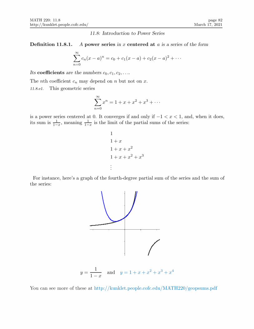


![KBR’s Transport Gasifier (TRIG™): Market Projection … Library/research/coal...Jindal Steel & Power TRIG for DRI Angul, India TRIG Pilot Plant South Korea [2011] Dongguan TRIG](https://static.documents.pub/doc/80x56/5aea25507f8b9a45568b5f98/kbrs-transport-gasifier-trig-market-projection-libraryresearchcoaljindal.jpg)


