The Kruskal and Wallis one-way analysis of variance by ranks or van der Waerden’snormal score test can be employed, if the data do not meet the assumptions for one-wayANOVA. Provided that significant differences were detected by the omnibus test, onemay be interested in applying post-hoc tests for pairwise multiple comparisons (such asNemenyi’s test, Dunn’s test, Conover’s test, van der Waerden’s test). Similarly, one-wayANOVA with repeated measures that is also referred to as ANOVA with unreplicatedblock design can also be conducted via the Friedman-Test or the Quade-test. The conse-quent post-hoc pairwise multiple comparison tests according to Nemenyi, Conover andQuade are also provided in this package. Finally Durbin’s test for a two-way balancedincomplete block design (BIBD) is also given in this package.
2 Comparison of multiple independent samples (One-factorialdesign)
2.1 Kruskal and Wallis test
The linear model of a one-way layout can be written as:
yi = µ+ αi + εi, (1)
with y the response vector, µ the global mean of the data, αi the difference to the meanof the i-th group and ε the residual error. The non-parametric alternative is the Kruskal
2
and Wallis test. It tests the null hypothesis, that each of the k samples belong to thesame population (H0 : Ri. = (n+ 1)/2). First, the response vector y is transformed intoranks with increasing order. In the presence of sequences with equal values (i.e. ties),mean ranks are designated to the corresponding realizations. Then, the test statistic canbe calculated according to Eq. 2:
H =
[12
n (n+ 1)
] [ k∑i=1
R2i
ni
]− 3 (n+ 1) (2)
with n =∑ki ni the total sample size, ni the number of data of the i-th group and R2
i
the squared rank sum of the i-th group. In the presence of many ties, the test statisticsH can be corrected using Eqs. 3 and 4
C = 1−∑i=ri=1
(t3i − ti
)n3 − n
, (3)
with ti the number of ties of the i-th group of ties.
H∗ = H/C (4)
The Kruskal and Wallis test can be employed as a global test. As the test statisticH is approximately χ2-distributed, the null hypothesis is withdrawn, if H > χ2
k−1;α.It should be noted, that the tie correction has only a small impact on the calculatedstatistic and its consequent estimation of levels of significance.
2.2 Kruskal-Wallis – post-hoc tests after Nemenyi
Provided, that the globally conducted Kruskal-Wallis test indicates significance (i.e.H0 is rejected, and HA : ’at least on of the k samples does not belong to the samepopulation’ is accepted), one may be interested in identifying which group or groupsare significantly different. The number of pairwise contrasts or subsequent tests thatneed to be conducted is m = k (k − 1) /2 to detect the differences between each group.Nemenyi proposed a test that originally based on rank sums and the application of thefamily-wise error method to control Type I error inflation, if multiple comparisons aredone. The Tukey and Kramer approach uses mean rank sums and can be employed forequally as well as unequally sized samples without ties (Sachs, 1997, p. 397). The nullhypothesis H0 : Ri = Rj is rejected, if a critical absolute difference of mean rank sumsis exceeded.
∣∣Ri − Rj∣∣ > q∞;k;α√2
√√√√[n (n+ 1)
12
] [1
ni+
1
nj
], (5)
where q∞;k;α denotes the upper quantile of the studentized range distribution. Thisinequality (5) leads to the same critical differences of rank sums (|Ri −Rj |) when mul-tiplied with n for α = [0.1, 0.5, 0.01], as reported in the tables of Wilcoxon and Wilcox
3
(1964, pp. 29–31). In the presence of ties the approach presented by Sachs (1997, p.395) can be employed (6), provided that (ni, nj , . . . , nk ≥ 6) and k ≥ 4.:
∣∣Ri − Rj∣∣ >√√√√ 1
Cχ2k−1;α
[n (n+ 1)
12
] [1
ni+
1
nj
], (6)
where C is given by Eq. 3. The function posthoc.kruskal.nemenyi.test does notevaluate the critical differences as given by Eqs. 5 and 6, but calculates the correspondinglevel of significance for the estimated statistics q and χ2, respectively.
In the special case, that several treatments shall only be tested against one controlexperiment, the number of tests reduces to m = k − 1. This case is given in section 2.8.
2.3 Examples using posthoc.kruskal.nemenyi.test
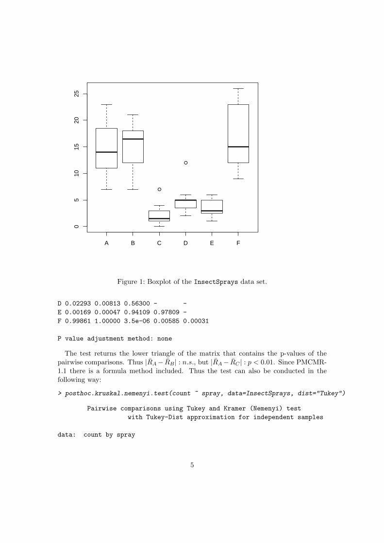
The function kruskal.test is provided with the library stats (R Core Team, 2013).The data-set InsectSprays was derived from a one factorial experimental design andcan be used for demonstration purposes. Prior to the test, a visualization of the data(Fig 1) might be helpful:
Based on a visual inspection, one can assume that the insecticides A, B, F differ fromC, D, E. The global test can be conducted in this way:
As the Kruskal-Wallis Test statistics is highly significant (χ2(5) = 54.69, p < 0.01),the null hypothesis is rejected. Thus, it is meaningful to apply post-hoc tests with thefunction posthoc.kruskal.nemenyi.test.
Pairwise comparisons using Tukey and Kramer (Nemenyi) test
with Tukey-Dist approximation for independent samples
data: count and spray
A B C D E
B 0.99961 - - - -
C 2.8e-05 5.7e-06 - - -
4
●
●
A B C D E F
05
1015
2025
Figure 1: Boxplot of the InsectSprays data set.
D 0.02293 0.00813 0.56300 - -
E 0.00169 0.00047 0.94109 0.97809 -
F 0.99861 1.00000 3.5e-06 0.00585 0.00031
P value adjustment method: none
The test returns the lower triangle of the matrix that contains the p-values of thepairwise comparisons. Thus |RA− RB| : n.s., but |RA− RC | : p < 0.01. Since PMCMR-1.1 there is a formula method included. Thus the test can also be conducted in thefollowing way:
Pairwise comparisons using Nemenyi-test with Chi-squared
approximation for independent samples
data: count and spray
A B C D E
B 0.99985 - - - -
C 0.00037 9.4e-05 - - -
D 0.08359 0.03812 0.73938 - -
E 0.01113 0.00391 0.97354 0.99070 -
F 0.99945 1.00000 6.2e-05 0.02955 0.00281
P value adjustment method: none
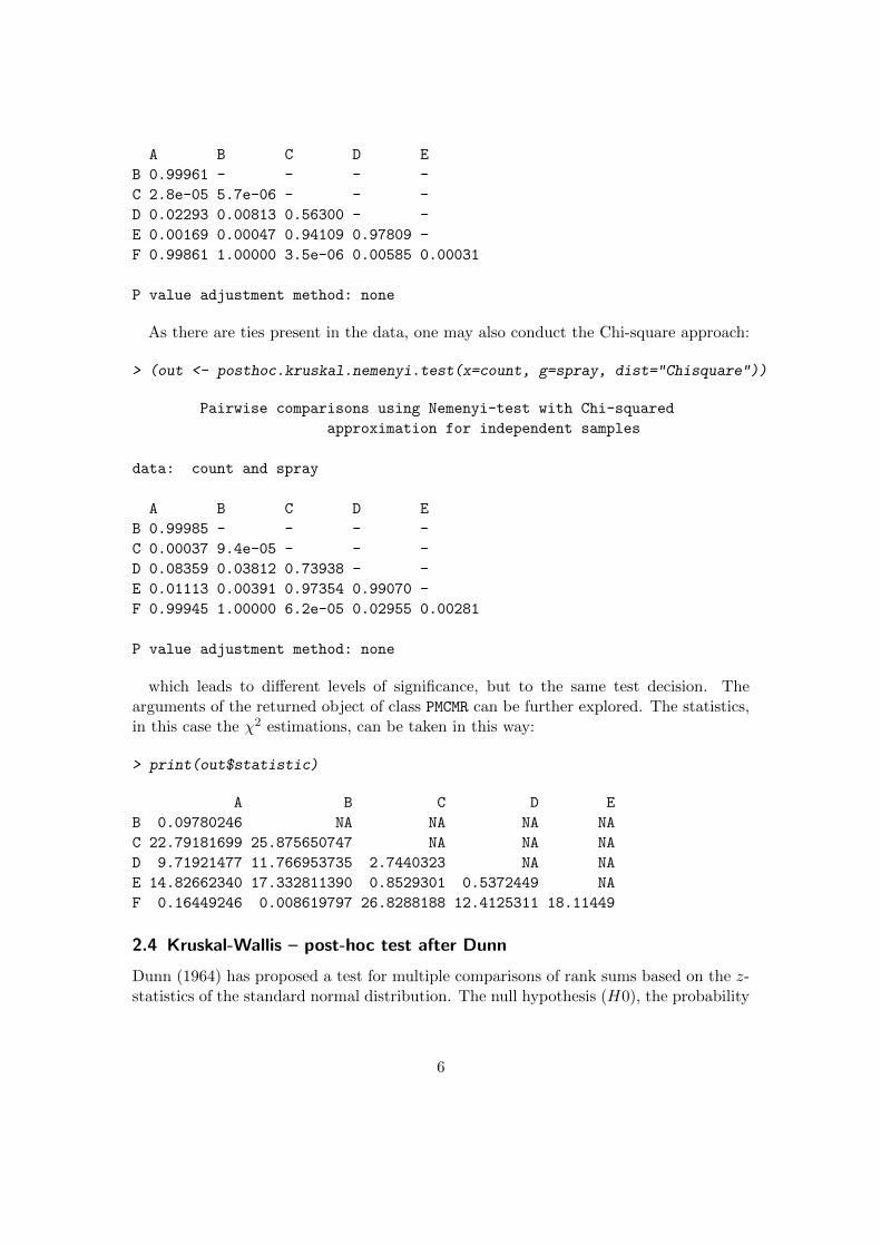
which leads to different levels of significance, but to the same test decision. Thearguments of the returned object of class PMCMR can be further explored. The statistics,in this case the χ2 estimations, can be taken in this way:
> print(out$statistic)
A B C D E
B 0.09780246 NA NA NA NA
C 22.79181699 25.875650747 NA NA NA
D 9.71921477 11.766953735 2.7440323 NA NA
E 14.82662340 17.332811390 0.8529301 0.5372449 NA
F 0.16449246 0.008619797 26.8288188 12.4125311 18.11449
2.4 Kruskal-Wallis – post-hoc test after Dunn
Dunn (1964) has proposed a test for multiple comparisons of rank sums based on the z-statistics of the standard normal distribution. The null hypothesis (H0), the probability
6
of observing a randomly selected value from the first group that is larger than a randomlyselected value from the second group equals one half, is rejected, if a critical absolutedifference of mean rank sums is exceeded:
∣∣Ri − Rj∣∣ > z1−α/2∗
√√√√[n (n+ 1)
12−B
] [1
ni+
1
nj
], (7)
with z1−α/2∗ the value of the standard normal distribution for a given adjusted α/2∗level depending on the number of tests conducted and B the correction term for ties,which was taken from Glantz (2012) and is given by Eq. 8:
B =
∑i=ri=1
(t3i − ti
)12 (n− 1)
(8)
The function posthoc.kruskal.dunn.test does not evaluate the critical differencesas given by Eqs. 7, but calculates the corresponding level of significance for the estimatedstatistics z, as adjusted by any method implemented in p.adjust to account for TypeI error inflation. It should be noted that Dunn (1964) originally used a Bonferroniadjustment of p-values. For this specific case, the test is sometimes referred as to theBonferroni-Dunn test.
Pairwise comparisons using Dunn's-test for multiple
comparisons of independent samples
data: count and spray
A B C D E
B 0.75448 - - - -
C 1.8e-06 3.6e-07 - - -
D 0.00182 0.00060 0.09762 - -
E 0.00012 3.1e-05 0.35572 0.46358 -
F 0.68505 0.92603 2.2e-07 0.00043 2.1e-05
P value adjustment method: none
The test returns the lower triangle of the matrix that contains the p-values of thepairwise comparisons. As p.adjust.method="none", the p-values are not adjusted.
7
Hence, there is a Type I error inflation that leads to a false positive discovery rate. Thiscan be solved by applying e.g. a Bonferroni-type adjustment of p-values.
Pairwise comparisons using Dunn's-test for multiple
comparisons of independent samples
data: count and spray
A B C D E
B 1.00000 - - - -
C 2.7e-05 5.5e-06 - - -
D 0.02735 0.00904 1.00000 - -
E 0.00177 0.00047 1.00000 1.00000 -
F 1.00000 1.00000 3.3e-06 0.00640 0.00031
P value adjustment method: bonferroni
2.6 Kruskal-Wallis – post-hoc test after Conover
Conover and Iman (1979) proposed a test that aims at having a higher test power thanthe tests given by inequalities 5 and 6:
∣∣Ri − Rj∣∣ > t1−α/2;n−k
√√√√s2 [n− 1− H∗n− k
] [1
ni+
1
nj
], (9)
with H∗ the tie corrected Kruskal-Wallis statistic according to Eq. 4 and t1−α/2;n−kthe t-value of the student-t-distribution. The variance s2 is given in case of ties by:
s2 =1
n− 1
[∑R2i − n
(n+ 1)2
4
](10)
The variance s2 simplifies to n (n+ 1) /12, if there are no ties present. AlthoughConover and Iman (1979) did not propose an adjustment of p-values, the functionposthoc.kruskal.conover.test has implemented methods for p-adjustment from thefunction p.adjust.
Pairwise comparisons using Conover's-test for multiple
comparisons of independent samples
data: count and spray
A B C D E
B 1.000 - - - -
C 5.6e-13 4.5e-14 - - -
D 4.7e-07 3.6e-08 0.021 - -
E 1.1e-09 8.5e-11 1.000 1.000 -
F 1.000 1.000 2.1e-14 1.7e-08 3.9e-11
P value adjustment method: bonferroni
2.8 Dunn’s multiple comparison test with one control
Dunn’s test (see section 2.4), can also be applied for multiple comparisons with onecontrol (Siegel and Castellan Jr., 1988):
∣∣R0 − Rj∣∣ > z1−α/2∗
√√√√[n (n+ 1)
12−B
] [1
n0+
1
nj
], (11)
9
where R0 denotes the mean rank sum of the control experiment. In this case thenumber of tests is reduced to m = k − 1, which changes the p-adjustment accordingto Bonferroni (or others). The function dunn.test.control employs this test, but theuser need to be sure that the control is given as the first level in the groupvector.
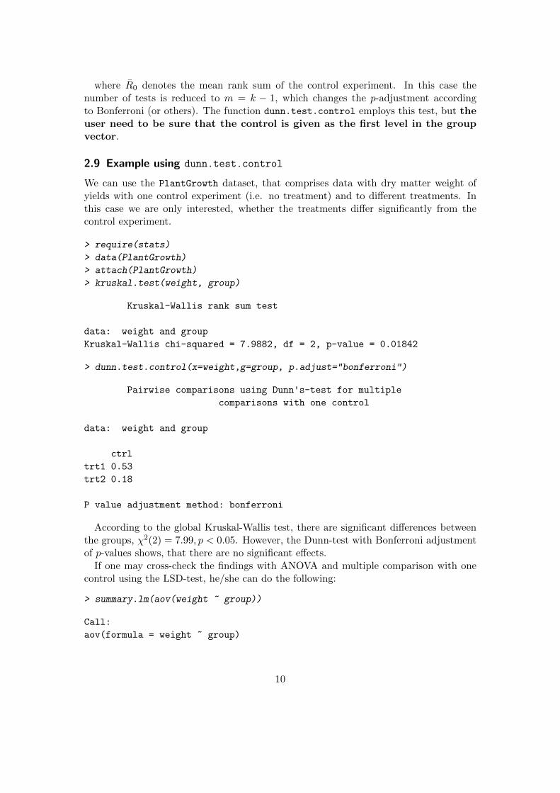
2.9 Example using dunn.test.control
We can use the PlantGrowth dataset, that comprises data with dry matter weight ofyields with one control experiment (i.e. no treatment) and to different treatments. Inthis case we are only interested, whether the treatments differ significantly from thecontrol experiment.
Pairwise comparisons using Dunn's-test for multiple
comparisons with one control
data: weight and group
ctrl
trt1 0.53
trt2 0.18
P value adjustment method: bonferroni
According to the global Kruskal-Wallis test, there are significant differences betweenthe groups, χ2(2) = 7.99, p < 0.05. However, the Dunn-test with Bonferroni adjustmentof p-values shows, that there are no significant effects.
If one may cross-check the findings with ANOVA and multiple comparison with onecontrol using the LSD-test, he/she can do the following:
F-statistic: 4.846 on 2 and 27 DF, p-value: 0.01591
The last line provides the statistics for the global test, i.e. there is a significanttreatment effect according to one-way ANOVA, F (2, 27) = 4.85, p < 0.05, η2 = 0.264.The row that starts with Intercept gives the group mean of the control, its standarderror, the t-value for testing H0 : µ = 0 and the corresponding level of significance. Thefollowing lines provide the difference between the averages of the treatment groups withthe control, where H0 : µ0 − µj = 0. Thus the trt1 does not differ significantly fromthe ctr, t = −1.331, p = 0.194. There is a significant difference between trt2 and ctr
as indicated by t = 1.772, p < 0.1.
2.10 van der Waerden test
The van der Waerden test can be used as an alternative to the Kruskal-Wallis test, ifthe data to not meet the requirements for ANOVA (Conover and Iman, 1979). Let theKruskal-Wallis ranked data denote Ri,j , then the normal scores Ai,j are derived from thestandard normal distribution according to Eq. 12.
Ai,j = φ−1(Ri,jn+ 1
)(12)
Let the sum of the i-th score denote Aj . The variance S2 is calculated as given in Eq.13.
S2 =1
n− 1
∑A2i,j (13)
Finally the test statistic is given by Eq. 14.
T =1
S2
k∑j=1
A2j
nj(14)
11
The test statistic T is approximately χ2-distributed and tested for significance on alevel of 1− α with df = k − 1.
2.11 Example using vanWaerden.test
> require(PMCMR)
> data(InsectSprays)
> attach(InsectSprays)
> vanWaerden.test(x=count, g=spray)
Van der Waerden normal scores test
data: count and spray
Van der Waerden chi-squared = 50.302, df = 5, p-value = 1.202e-09
2.12 post-hoc test after van der Waerden for multiple pairwise comparisons
Provided that the global test according to van der Waerden indicates significance, mul-tiple comparisons can be done according to the inequality 15.
‖Aini− Ajnj‖ > t1−α/2∗;n−k
√√√√S2n− 1− Tn− k
(1
ni+
1
nj
)(15)
The test given in Conover and Iman (1979) does not adjust p-values. However, thefunction has included the methods for p-value adjustment as given by p.adjust.
Pairwise comparisons using van der Waerden normal scores test for
multiple comparisons of independent samples
data: count and spray
A B C D E
B 0.6366 - - - -
C 6.9e-12 9.8e-13 - - -
D 9.0e-06 1.5e-06 0.0008 - -
E 5.5e-08 8.1e-09 0.0316 0.1919 -
F 0.2323 0.4675 5.0e-14 8.6e-08 4.1e-10
P value adjustment method: none
12
3 Test of k independent samples against an ordered alternative
3.1 Jonckheere-Terpstrata test
For testing k independent samples against an ordered alternative (e.g. k groups withincreasing doses of treatment), the test according to Jonckheere (1954) can be employed.Both, the null and alternative hypothesis can be formulated as population medians (θi)for k populations (k > 2). Thus the null hypothesis, H0 : θ1 = θ2 = . . . = θk is testede.g. in the one-sided case against the alternative, HA : θ1 ≤ θ2 ≤ . . . ≤ θk, with at leastone strict inequality.
The statistic J is calculated according to Eq. 16.
J =k−1∑i=1
k∑j=i+1
Uij (16)
where Uij is defined as:
Uij =ni∑s=1
nj∑t=1
ψ (Xjt −Xis) (17)
with
ψ (u) =
1 ∀ u > 0
1/2 ∀ u = 00 ∀ u < 0
(18)
The mean µJ is given by
µJ =N2 −
∑ki=1 n
2i
4(19)
and the variance σJ is defined as
σJ =
√N2 (2N + 3)−
∑ki=1 n
2i (2ni + 3)
72. (20)
The z-value of the standard normal distribution is calculated as:
z =J − µJσJ
(21)
For a one-sided test, the H0 is rejected, if z > z1−α/2. The implemented function cantest for monotonic trend (two-sided), increasing or decreasing trend (one-sided).
13
3.2 Example using jonckheere.test
> ## Example from Sachs (1997, p. 402)
> require(PMCMR)
> x <- c(106, 114, 116, 127, 145, 110, 125,
+ 143, 148, 151, 136, 139, 149, 160,
+ 174)
> g <- as.factor(c(rep(1,5), rep(2,5), rep(3,5)))
> levels(g) <- c("A", "B", "C")
> jonckheere.test(x , g, "increasing")
Jonckheere-Terpstrata test
data: x and g
Jonckheere z-value = 2.2716, p-value = 0.01156
alternative hypothesis: increasing
> rm(x,g)
4 Comparison of multiple joint samples (Two-factorialunreplicated complete block design)
4.1 Friedman test
The linear model of a two factorial unreplicated complete block design can be writtenas:
yi,j = µ+ αi + πj + εi,j (22)
with πj the j-th level of the block (e.g. the specific response of the j-th test person).The Friedman test is the non-parametric alternative for this type of k dependent treat-ment groups with equal sample sizes. The null hypothesis, H0 : F (1) = F (2) = . . . =F (k) is tested against the alternative hypothesis: at least one group does not belongto the same population. The response vector y has to be ranked in ascending orderseparately for each block πj : j = 1, . . .m. After that, the statistics of the Friedman testis calculated according to Eq. 23:
χ2R =
[12
nk (k + 1)
k∑i=1
Ri
]− 3n (k + 1) (23)
The Friedman statistic is approximately χ2-distributed and the null hypothesis isrejected, if χR > χ2
k−1;α.
14
4.2 Friedman – post-hoc test after Nemenyi
Provided that the Friedman test indicates significance, the post-hoc test according toNemenyi (1963) can be employed (Sachs, 1997, p. 668). This test requires a balanced de-sign (n1 = n2 = . . . = nk = n) for each group k and a Friedman-type ranking of the data.The inequality 24 was taken from Demsar (2006, p. 11), where the critical differencerefer to mean rank sums (
∣∣Ri − Rj∣∣):∣∣Ri − Rj∣∣ > q∞;k;α√
2
√k (k + 1)
6n(24)
This inequality leads to the same critical differences of rank sums (|Ri −Rj |) whenmultiplied with n for α = [0.1, 0.5, 0.01], as reported in the tables of Wilcoxon andWilcox (1964, pp. 36–38). Likewise to the posthoc.kruskal.nemenyi.test the func-tion posthoc.friedman.nemenyi.test calculates the corresponding levels of signifi-cance and the generic function print depicts the lower triangle of the matrix thatcontains these p-values. The test according to Nemenyi (1963) was developed to ac-count for a family-wise error and is already a conservative test. This is the reason, whythere is no p-adjustment included in the function.
4.3 Example using posthoc.friedman.nemenyi.test
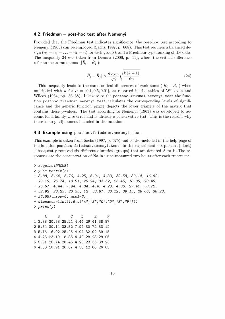
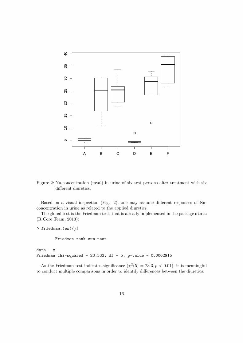
This example is taken from Sachs (1997, p. 675) and is also included in the help page ofthe function posthoc.friedman.nemenyi.test. In this experiment, six persons (block)subsequently received six different diuretics (groups) that are denoted A to F. The re-sponses are the concentration of Na in urine measured two hours after each treatment.
As the Friedman test indicates significance (χ2(5) = 23.3, p < 0.01), it is meaningfulto conduct multiple comparisons in order to identify differences between the diuretics.
16
> posthoc.friedman.nemenyi.test(y)
Pairwise comparisons using Nemenyi multiple comparison test
with q approximation for unreplicated blocked data
data: y
A B C D E
B 0.1880 - - - -
C 0.0917 0.9996 - - -
D 0.9996 0.3388 0.1880 - -
E 0.0395 0.9898 0.9996 0.0917 -
F 0.0016 0.6363 0.8200 0.0052 0.9400
P value adjustment method: none
According to the Nemenyi post-hoc test for multiple joint samples, the treatment Fbased on the Na diuresis differs highly significant (p < 0.01) to A and D, and E differssignificantly (p < 0.05) to A. Other contrasts are not significant (p > 0.05). This is thesame test decision as given by (Sachs, 1997, p. 675).
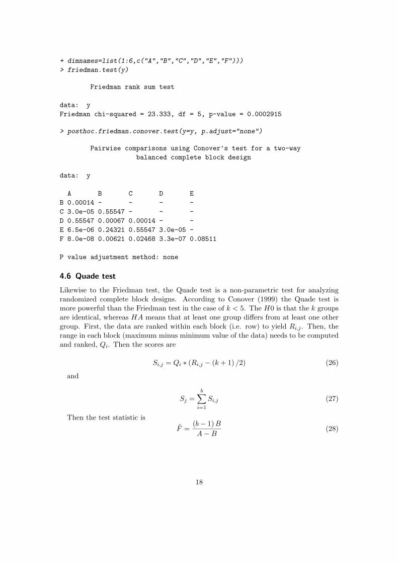
4.4 Friedman – post-hoc test after Conover
Conover (1999) proposed a post-hoc test for pairwise comparisons, if Friedman-Test indi-cated significance. The absolute difference between two group rank sums are significantlydifferent, if the following inequality is satisfied:
|Ri −Rj | > t1−α/2;(n−1)(k−1)
√√√√√2k
(1− χ2
Rn(k−1)
)(∑ni=1
∑kj=1R
2i,j −
nk(k+1)2
4
)(k − 1) (n− 1)
(25)
Although Conover (1999) originally did not include a p-adjustment, the function hasincluded the methods as given by p.adjust, because it is a very liberal test. So it is upto the user, to apply a p-adjustment or not, when using this function.
Pairwise comparisons using Conover's test for a two-way
balanced complete block design
data: y
A B C D E
B 0.00014 - - - -
C 3.0e-05 0.55547 - - -
D 0.55547 0.00067 0.00014 - -
E 6.5e-06 0.24321 0.55547 3.0e-05 -
F 8.0e-08 0.00621 0.02468 3.3e-07 0.08511
P value adjustment method: none
4.6 Quade test
Likewise to the Friedman test, the Quade test is a non-parametric test for analyzingrandomized complete block designs. According to Conover (1999) the Quade test ismore powerful than the Friedman test in the case of k < 5. The H0 is that the k groupsare identical, whereas HA means that at least one group differs from at least one othergroup. First, the data are ranked within each block (i.e. row) to yield Ri,j . Then, therange in each block (maximum minus minimum value of the data) needs to be computedand ranked, Qi. Then the scores are
Si,j = Qi ∗ (Ri,j − (k + 1) /2) (26)
and
Sj =b∑i=1
Si,j (27)
Then the test statistic is
F =(b− 1)B
A−B(28)
18
with
A =b∑i=1
k∑j=1
S2i,j
B =1
b
k∑i=1
S2j
The test statistic F is tested against the F -quantile for a given α with df1 = k − 1and df2 = (b− 1) (k − 1). This is equivalent to a two-way ANOVA on the scores Si,j .
4.7 Quade – posthoc tests
The package PMCMR offers two posthoc tests following a significant Quade test. Inequality29 was taken from Heckert and Filliben (2003) and uses the student-t distribution.
|Si − Sj | > t1−α/2∗,(b−1)(k−1)
√2b (A−B)
(b− 1) (k − 1)(29)
Inequality 30 was taken from the manual of STATService 2.0 (Parejo et al., 2012) anduses the standard normal distribution.∣∣∣∣∣ Wi
ni (ni + 1) /2− Wj
nj (nj + 1) /2
∣∣∣∣∣ > z1−α/2∗
√k (k + 1) (2n+ 1) (k − 1)
18n (n+ 1)(30)
with
Wj =b∑i=1
(Qi ∗Ri,j) (31)
The calculated p-values can be adjusted to control Type I error inflation with themethods as given in p.adjust.
4.8 Example using posthoc.quade.test
> ## Conover (1999, p. 375f):
> ## Numbers of five brands of a new hand lotion sold in seven stores
> ## during one week.
> y <- matrix(c( 5, 4, 7, 10, 12,
+ 1, 3, 1, 0, 2,
+ 16, 12, 22, 22, 35,
+ 5, 4, 3, 5, 4,
+ 10, 9, 7, 13, 10,
+ 19, 18, 28, 37, 58,
+ 10, 7, 6, 8, 7),
+ nrow = 7, byrow = TRUE,
+ dimnames =
19
+ list(Store = as.character(1:7),
+ Brand = LETTERS[1:5]))
> y
Brand
Store A B C D E
1 5 4 7 10 12
2 1 3 1 0 2
3 16 12 22 22 35
4 5 4 3 5 4
5 10 9 7 13 10
6 19 18 28 37 58
7 10 7 6 8 7
> quade.test(y)
Quade test
data: y
Quade F = 3.8293, num df = 4, denom df = 24, p-value = 0.01519
Provided that the omnibus test of Durbin indicates, that at least one group differs fromanother group, multiple comparisons can be conducted according to Inequality 34
‖Rj −Ri‖ > t1−α/2∗,bk−b−t+1
√(A− C) 2r
bk − b− t+ 1
(1− χ2
b ∗ (k − 1)
)(34)
The p-values can be adjusted with p.adjust.
5.4 Example using posthoc.durbin.test
> posthoc.durbin.test(y, p.adj="none")
Pairwise comparisons using Durbin's test for a two-way
balanced incomplete block design
data: y
A B C D E F
B 0.4379 - - - - -
C 0.0114 0.0035 - - - -
D 0.0035 0.0012 0.4379 - - -
E 0.0400 0.0114 0.4379 0.1411 - -
F 0.1411 0.0400 0.1411 0.0400 0.4379 -
G 0.4379 0.1411 0.0400 0.0114 0.1411 0.4379
P value adjustment method: none
6 Auxiliary functions
The package PMCMR comes with a print.PMCMR and a summary.PMCMR function:
> print(posthoc.durbin.test(y, p.adj="none"))
22
Pairwise comparisons using Durbin's test for a two-way
balanced incomplete block design
data: y
A B C D E F
B 0.4379 - - - - -
C 0.0114 0.0035 - - - -
D 0.0035 0.0012 0.4379 - - -
E 0.0400 0.0114 0.4379 0.1411 - -
F 0.1411 0.0400 0.1411 0.0400 0.4379 -
G 0.4379 0.1411 0.0400 0.0114 0.1411 0.4379
P value adjustment method: none
> summary(posthoc.durbin.test(y, p.adj="none"))
Pairwise comparisons using Durbin's test for a two-way
balanced incomplete block design
data: y
P value adjustment method: none
H0 statistic p.value
1 A = B 0.8164966 0.4379
2 A = C 3.2659863 0.0114
3 A = D 4.0824829 0.0035
4 A = E 2.4494897 0.0400
5 A = F 1.6329932 0.1411
6 A = G 0.8164966 0.4379
7 B = C 4.0824829 0.0035
8 B = D 4.8989795 0.0012
9 B = E 3.2659863 0.0114
10 B = F 2.4494897 0.0400
11 B = G 1.6329932 0.1411
12 C = D 0.8164966 0.4379
13 C = E 0.8164966 0.4379
14 C = F 1.6329932 0.1411
15 C = G 2.4494897 0.0400
16 D = E 1.6329932 0.1411
17 D = F 2.4494897 0.0400
18 D = G 3.2659863 0.0114
19 E = F 0.8164966 0.4379
23
20 E = G 1.6329932 0.1411
21 F = G 0.8164966 0.4379
Furthermore, the function get.pvalues was included, to extract the p-values from anPMCMR object or an pairwise.htest object. The output of get.pvalues is a named nu-meric vector, where each element is named after the corresponding pairwise comparison.It can be further processed with multcompLetters from the package multcompView tofind and indicate homogeneous groups for a given level of significance. This can be usedto create plots (Fig. 3) or tables (Table 1) with xtable.
> require(xtable)
> require(multcompView)
> data(InsectSprays)
> attach(InsectSprays)
> out <- posthoc.kruskal.dunn.test(count ~ spray, p.adjust="bonf")
Table 1: Mean ranks (Rj) of the InsectSprays data set. Different letters (M) indicatesignificant differences (p < 0.05) according to the Bonferroni-Dunn test (seeChap. 2.4).
Demsar J (2006). “Statistical comparisons of classifiers over multiple data sets.” Journalof Machine Learning Research, 7, 1–30.
Dunn OJ (1964). “Multiple comparisons using rank sums.” Technometrics, 6, 241–252.
Glantz SA (2012). Primer of biostatistics. 7 edition. McGraw Hill, New York.
Heckert NA, Filliben JJ (2003). “Dataplot Reference Manual, Volume 2: Let Subcom-mands and Library Functions.” Technical Report 148, National Institute of Standardsand Technology.
Jonckheere AR (1954). “A distribution-free k-sample test against ordered alternatives.”Biometrica, 41, 133–145.
Nemenyi P (1963). Distribution-free Multiple Comparisons. Ph.D. thesis, PrincetonUniversity.
Parejo JA, Garcıa J, Ruiz-Cortes A, Riquelme JC (2012). “STATService: Herramientade analisis estadıstico como soporte para la investigacion con Metaheurısticas. Ac-tas del VIII Congreso Expanol sobre Metaheurısticas, Algoritmos Evolutivos y Bio-inspirados.”
R Core Team (2013). R: A language and environement for statistical computing. Vienna,Austria. URL http://www.R-project.org/.
Sachs L (1997). Angewandte Statistik. 8 edition. Springer, Berlin.
Siegel S, Castellan Jr NJ (1988). Nonparametric Statistics for The Behavioral Sciences.2nd edition. McGraw-Hill, New York.
25
Wilcoxon F, Wilcox RA (1964). Some rapid approximate statistical procedures. LederleLaboratories, Pearl River.
26
> require(multcompView)
> data(InsectSprays)
> attach(InsectSprays)
> out <- posthoc.kruskal.dunn.test(count ~ spray, p.adjust="bonf")
> xx <- barplot(Rj.mean, ylim=c(0, 1.2* max(Rj.mean)),
+ xlab="Spray", ylab="Mean rank")
> yy <- Rj.mean + 3
> text(xx, yy, lab=out.mcV$Letters)
> detach(InsectSprays)
A B C D E F
Spray
Mea
n ra
nk
010
2030
4050
60
aa
b
b
b
a
Figure 3: Barplot of mean ranks of the InsectSprays data set. Different letters indicatesignificant differences (p < 0.05) according to the Bonferroni-Dunn test (seeChap. 2.4).