www.elsevier.com/locate/palaeo

Palaeogeography, Palaeoclimatology, P

The palaeoclimatology, palaeoecology and palaeoenvironmental

analysis of mass extinction events

Richard J. Twitchett

School of Earth, Ocean and Environmental Sciences, University of Plymouth, Drake Circus, Plymouth, PL4 8AA, UK

Received 1 December 2004; received in revised form 22 April 2005; accepted 23 May 2005

Abstract

Although there is a continuum in magnitude of diversity loss between the smallest and largest biotic crisis, typically most

authors refer to the largest five Phanerozoic events as bmass extinctionsQ. In the past 25 years the study of these mass extinction

events has increased dramatically, with most focus being on the Cretaceous–Tertiary (K–T) event, although study of the end-

Permian event (in terms of research output) is likely to surpass that of the K–T in the next few years. Many aspects of these events

are still debated and there is no common cause or single set of climatic or environmental changes common to these five events,

although all are associated with evidence for climatic change. The supposed extinction-causing environmental changes resulting

from extraterrestrial impact are, at best, equivocal and are unlikely to have been of sufficient intensity or geographic extent to

cause global extinction. The environmental consequences of rapid global warming (such as ocean stagnation, reduced upwelling

and loss of surface productivity) are considered to have been particularly detrimental to the biosphere in the geological past. The

first phase of the Late Ordovician event is clearly linked to rapid global cooling. Palaeoecological studies have demonstrated that

feeding mechanism is a key trait that enhances survival chances, with selective detritivores and omnivores usually faring better

than suspension feeders or grazers. This indicates that primary productivity collapse and consequent lack of food supply is a key

proximate cause of extinction. Typically, this low productivity state continues for several hundred thousand years and is

associated with widespread stunting of marine organisms (the Lilliput effect) and low-biomass ecosystems. Rebuilding of the

marine ecosystem is an important process, and a number of models have been constructed that can be used for comparative

purposes (e.g., to understand variation in rates of recovery between events, or between different regions within the same event).

Understanding the extinction and recovery processes in ancient events, especially those associated with global warming, may be

crucial to managing the present biodiversity crisis. Yet, as many aspects of these mass extinction events remain little understood,

there is still much work to do.

D 2005 Elsevier B.V. All rights reserved.

Keywords: Mass extinction; Ordovician; Devonian; Permian; Triassic; Cretaceous; Paleoecology

0031-0182/$ - s

doi:10.1016/j.pa

E-mail addre

alaeoecology 232 (2006) 190–213

ee front matter D 2005 Elsevier B.V. All rights reserved.

laeo.2005.05.019

ss: rtwitchett@plymouth.ac.uk.

R.J. Twitchett / Palaeogeography, Palaeoclimatology, Palaeoecology 232 (2006) 190–213 191

Contents

. . . . . . 191

. . . . . . 192

. . . . . . 193

. . . . . . 193

. . . . . . 195

. . . . . . 196

. . . . . . 196

. . . . . . 197

. . . . . . 197

. . . . . . 198

. . . . . . 198

. . . . . . 201

. . . . . . 201

. . . . . . 202

. . . . . . 203

. . . . . . 205

. . . . . . 207

1. Introduction . . . . . . . . . . . . . . . . . . . . . . . . . . . . . . . . . . . . . . . . . . . . . .

2. Brief history of mass extinction studies . . . . . . . . . . . . . . . . . . . . . . . . . . . . . . .

3. Palaeoclimates and extinction events . . . . . . . . . . . . . . . . . . . . . . . . . . . . . . . . .

3.1. Global warming . . . . . . . . . . . . . . . . . . . . . . . . . . . . . . . . . . . . . . . .

3.2. Global cooling . . . . . . . . . . . . . . . . . . . . . . . . . . . . . . . . . . . . . . . . .

4. Palaeoenvironments and extinction events . . . . . . . . . . . . . . . . . . . . . . . . . . . . . .

4.1. Palaeoenvironmental bias . . . . . . . . . . . . . . . . . . . . . . . . . . . . . . . . . . .

4.2. Sea-level fall . . . . . . . . . . . . . . . . . . . . . . . . . . . . . . . . . . . . . . . . . .

4.3. Sea level rise . . . . . . . . . . . . . . . . . . . . . . . . . . . . . . . . . . . . . . . . .

4.4. Oceanic anoxia . . . . . . . . . . . . . . . . . . . . . . . . . . . . . . . . . . . . . . . .

4.5. Bolide impact . . . . . . . . . . . . . . . . . . . . . . . . . . . . . . . . . . . . . . . . .

5. Palaeoecology of extinction events . . . . . . . . . . . . . . . . . . . . . . . . . . . . . . . . . .

5.1. Selectivity . . . . . . . . . . . . . . . . . . . . . . . . . . . . . . . . . . . . . . . . . . .

5.2. Biotic recovery . . . . . . . . . . . . . . . . . . . . . . . . . . . . . . . . . . . . . . . .

5.2.1. The Kauffman–Erwin (1995) model . . . . . . . . . . . . . . . . . . . . . . . . .

5.2.2. A new recovery model?. . . . . . . . . . . . . . . . . . . . . . . . . . . . . . . .

5.3. Size change (the Lilliput Effect) . . . . . . . . . . . . . . . . . . . . . . . . . . . . . . . .

6. Summary . . . . . . . . . . . . . . . . . . . . . . . . . . . . . . . . . . . . . . . . . . . . . . .

. . . . . . 208

Acknowledgements . . . . . . . . . . . . . . . . . . . . . . . . . . . . . . . . . . . . . . . . . . . . . . . . . . 209

References . . . . . . . . . . . . . . . . . . . . . . . . . . . . . . . . . . . . . . . . . . . . . . . . . . . . . . . 209

1. Introduction

Most of the species that have ever lived on Earth

are extinct. Understanding the processes of extinction

is therefore crucial to understanding the evolution of

the biosphere. In addition, the extinction of certain

fossil taxa, and their subsequent replacement by

others, also makes possible the biostratigraphic corre-

lation of sedimentary rocks, which was first proposed

by William Smith more than 200 years ago and which

is still the primary means of correlation and relative

dating used today. Finally, an appreciation of the

causes and consequences of previous extinction epi-

sodes may assist with our management of the present

day biodiversity crisis.

Analysis of the fossil record indicates that extinction

rates, at species, genus, or higher taxonomic level, have

not been constant through time (e.g., Benton, 1995).

Episodes of elevated extinction typically occur at or

near period or stage boundaries: a consequence of the

original biostratigraphic definitions of these time inter-

vals and a desire to place boundaries bwhere something

happenedQ (e.g., Newell, 1962; McLaren, 1970). Dur-

ing these events there is apparently synchronous, or

near synchronous, often rapid, global extinction of

many different animal and/or plant taxa. The largest

of these events are referred to as bmassQ extinction

events, although this is a rather poorly defined term

(see discussions in Hallam and Wignall, 1997; Ben-

ton, 2003). Most authors accept five such mass ex-

tinction events: the Late Ordovician, Late Devonian

(Frasnian–Famennian), Late Permian, Late Triassic

and end-Cretaceous (K–T) events (e.g., McGhee et

al., 2004). However, some have long referred to an

episode of bmass extinctionQ in the Cambrian (e.g.,

Newell, 1962), whereas others refer to the present

day biotic crisis as the bsixthQ mass extinction event

(e.g., Benton, 2003, p. 284). In terms of the magni-

tude of diversity loss, a clear continuum exists be-

tween the smallest biotic crisis and the largest bmassQextinction event (Raup, 1991). The term bmassQ ex-tinction is thus arbitrary and somewhat redundant.

Herein, it is used sparingly and only for those five

ancient extinction events listed above.

Today, extinction studies encompass a wide spectrum

of geological activity, including palaeontological, sedi-

mentological, geochemical, geophysical and stratigraph-

ic analysis, as well as palaeoclimatology and other

studies involving numerical (computer) modelling. The

aim of this present work is to provide an overview of

R.J. Twitchett / Palaeogeography, Palaeoclimatology, Palaeoecology 232 (2006) 190–213192

some recent advances in mass extinction studies provid-

ed by palaeoclimate, palaeoenvironmental and palaeoe-

cological data, and an outline of where such studies may

lead us in the near future.Many substantial volumes have

been written in recent years detailing the individual

events themselves, such as Alvarez (1997), Benton

(2003), Erwin (1993), and McGhee (1996). Herein,

the focus will be broader, outlining general similarities

and differences between the events, rather than provid-

ing a detailed description of each.

2. Brief history of mass extinction studies

The earliest representation of the diversity of life

through the Phanerozoic, including (possibly) some of

1970-1974 1975-1979 1980-1984 1985-19

10

20

30

50

70

40

60

80

90

100

110

120

(46)

(10)(13)(1)

Num

ber

of p

ublic

atio

ns p

er e

vent

per

5 y

ear

inte

rval

Key:

Late Ordovician event Late Devonian (Frasnian-Famennian) eLate Permian eventLate Triassic event

Cretaceous-Tertiary event

Sum of all events

1970-1974 1975-1979 1980-1984 1985-19

4

8

12

16

(9)

(4)(3)

(0)

A

B

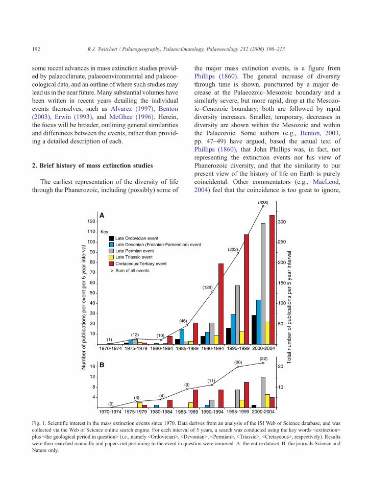
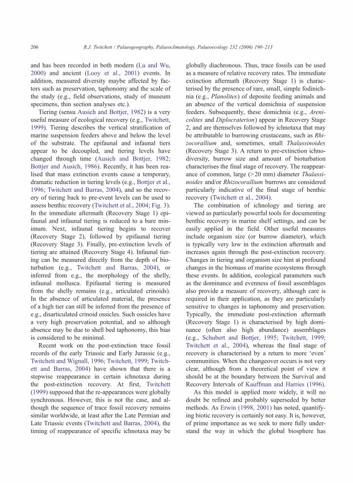
Fig. 1. Scientific interest in the mass extinction events since 1970. Data de

collected via the Web of Science online search engine. For each interval o

plus bthe geological period in questionN (i.e., namely bOrdovicianN, bDev

were then searched manually and papers not pertaining to the event in ques

Nature only.

the major mass extinction events, is a figure from

Phillips (1860). The general increase of diversity

through time is shown, punctuated by a major de-

crease at the Palaeozoic–Mesozoic boundary and a

similarly severe, but more rapid, drop at the Mesozo-

ic–Cenozoic boundary; both are followed by rapid

diversity increases. Smaller, temporary, decreases in

diversity are shown within the Mesozoic and within

the Palaeozoic. Some authors (e.g., Benton, 2003,

pp. 47–49) have argued, based the actual text of

Phillips (1860), that John Phillips was, in fact, not

representing the extinction events nor his view of

Phanerozoic diversity, and that the similarity to our

present view of the history of life on Earth is purely

coincidental. Other commentators (e.g., MacLeod,

2004) feel that the coincidence is too great to ignore,

89 1990-1994 1995-1999 2000-2004

50

100

150

200

250

300

(338)

(222)

(129)T

otal

num

ber

of p

ublic

atio

ns p

er 5

yea

r in

terv

al

vent

89 1990-1994 1995-1999 2000-2004

10

20

(11)

(20)(22)

rives from an analysis of the ISI Web of Science database, and was

f 5 years, a search was conducted using the key words bextinctionN

onianN, bPermianN, bTriassicN, bCretaceousN, respectively). Results

tion were removed. A: the entire dataset. B: the journals Science and

R.J. Twitchett / Palaeogeography, Palaeoclimatology, Palaeoecology 232 (2006) 190–213 193

and that there is more to this figure than is detailed in

its accompanying text.

Regardless of the true intentions behind the figure

of Phillips (1860), the study of mass extinction events

largely languished untouched until the 1950s and 60s,

with Schindewolf’s theories that catastrophic extinc-

tion could be caused by peaks in the influx of cosmic

radiation (e.g., Schindewolf, 1963). This absence of

scientific debate concerning extinction events is usu-

ally attributed to the prevalence of Uniformitarianism

in the geological sciences, since the publication of

Charles Lyell’s Principles of Geology in the early

1830s (e.g., McLaren, 1970; Pope et al., 1998; Ben-

ton, 2003). In particular, both Lyell and Darwin (and

most subsequent authors of the late 19th and early

20th centuries) considered that evolutionary change

was gradual and that apparent major extinction events,

such as the K–T boundary, could only be explained by

significant gaps in the fossil record (Pope et al., 1998).

Despite a few perceptive comments to the contrary

(e.g., McLaren, 1970), this view was not seriously

challenged until relatively recently: e.g., Raup (1978)

showed that, if all extinction was gradual and uniform,

then the time gap at the Permian–Triassic boundary

must represent (an impossible) 85 million years.

Using the on-line ISI Web of Science database, the

more recent surge of scientific interest in mass extinc-

tion events can be clearly demonstrated (Fig. 1).

Although these data represent a small, biased sample

of total scientific output over the time period in ques-

tion, (e.g., they ignore published conference proceed-

ings), several broad trends are apparent. First, with

one or two minor exceptions, each event records a

continuous increase in scientific interest (i.e., number

of publications per five-year interval) over the past 30

years. Second, there were very low levels of interest in

these events prior to the 1980s, which supports the

widely held view (e.g., Benton, 2003, p. 96) that the

publication of the impact hypothesis of Alvarez et al.

(1980) was a key element in kick-starting the present-

day interest in extinction studies. Certainly, publica-

tions concerning the end-Cretaceous extinction event

have dominated output since (Fig. 1), but it’s not

obvious from the data that Alvarez et al. (1980)

sparked interest in the other events. Other factors,

such as technological advances (in the speed and

power of computers, the precision of isotope analyses

etc.) have also played a role. Finally, it is also clear

from the data that the different events have attracted

different levels of interest through time. For example,

interest in the Late Permian event remained relatively

low key until the early 1990s, while (apparently) the

Late Triassic event did not begin to attract significant

scientific attention until the late 1990s. Of the indi-

vidual events, only the K–T data seem to be recording

a decline in the rate of scientific output: if these trends

continue then the Late Permian event will surpass the

K–T event in terms of global scientific interest in the

next five years. Evidence that interest in the K–T

event has already peaked is clear from the publica-

tions record of the leading scientific journals Science

and Nature (Fig. 1B).

3. Palaeoclimates and extinction events

Although it is often difficult to prove and cause and

effect relationship, the author considers that all major

extinction episodes of the past resulted, ultimately,

from changes in climate, induced by earthbound pro-

cesses such as extensive volcanism, and that the case

for an extraterrestrial cause of global extinction is, at

best, unconvincing (see discussion below). Three types

of climate change could potentially cause global ex-

tinction: rapid global cooling, rapid global warming, or

rapid fluctuations of warming and cooling. However,

the case for the latter mechanism as an extinction

trigger is considerably weakened by data from the

recent geological past, showing that no major marine

extinction occurred with the advance and retreat of the

Pleistocene ice caps (Newell, 1962; Valentine and

Jablonski, 1991). Thus, only the first two mechanisms

are considered below. The rapidity of the change is

considered important, as most organisms should be

able to cope with slow change over millions of years.

3.1. Global warming

Understanding the causes and consequences of an-

cient episodes of global warming has obvious signifi-

cance for debates concerning current climate change.

Global warming is associated with the second phase of

the Late Ordovician event (e.g., Brenchley et al., 2003

and refs. therein), the Late Permian event (Benton and

Twitchett, 2003; Kidder and Worsley, 2003), and the

Triassic–Jurassic event (McElwain et al., 1999; Tanner

R.J. Twitchett / Palaeogeography, Palaeoclimatology, Palaeoecology 232 (2006) 190–213194

et al., 2004). A number of palaeo-proxies for global

warming exist, and comprise (a) direct proxies of rel-

ative temperature rise and (b) indirect proxies of rela-

tive increase in known greenhouse gases such as CO2

and CH4. The former category includes the oxygen

isotope record of seawater carbonates (e.g., Brenchley

et al., 2003) and the morphology of palaeosols (e.g.,

Retallack, 1999). The latter category includes the sto-

matal index of fossil plants (e.g., McElwain et al.,

1999), which may be considered a proxy for atmo-

spheric CO2 levels; and large negative shifts in the

d13C carbonate record, which many have interpreted

as indicating significant methane venting (e.g., Erwin,

1993; Krull and Retallack, 2000), although this is

debatable (Kump, 1991; Berner, 2002).

It is assumed that geologically rapid global warm-

ing requires some unusual trigger, resulting in a major

input of greenhouse gases into the atmosphere. The

common association of mass extinction events, flood

basalt eruptions and evidence for global warming

have led some authors to propose that the flood

basalts provide the trigger, through the venting of

large amounts CO2 (e.g., Wignall, 2001). For the

Late Permian and Late Triassic events, it is further

assumed that this initial phase of global warming

leads to the dissociation of gas hydrates in the shallow

shelf seas and/or high latitude permafrost, resulting in

methane release. This exacerbates the global warming,

leading to further temperature rise, further methane

release, and a runaway greenhouse effect (e.g., Benton

and Twitchett, 2003).

However, evidence for this scenario is circumstan-

tial at best, relying on accurate dating of the flood

basalt province and the presence of a large, otherwise

unexplained, negative shift in the d13C carbonate

record (as evidence of methane release). Caution is

required as large negative shifts could be caused by

other mechanisms, such as productivity crash (Kump,

1991) or undetected diagenesis (Mii et al., 1997) for

marine carbonates. A negative shift in bulk organic

matter is likely due to a change in organic matter

source, such as a reduction in the relative contribution

of material from higher plants (Foster et al., 1997).

Volcanically vented CO2 is also enriched in 12C.

Recently, Berner (2002) noted that, regarding the

end-Permian event, it is not possible to reject all of

these other causes and the d13C record was likely

driven by methane release associated with mass mor-

tality and volcanic degassing. Thus, methane venting

is a possible explanation for the observed negative

shift in d13C. The shift itself should not be regarded asunequivocal evidence of methane flux to the atmo-

sphere. Very large d13C excursions in the aftermath of

the end-Permian event are almost certainly not the

result of methane venting (Payne et al., 2004).

Although more work on understanding and mod-

elling the triggers of catastrophic global warming are

required, the environmental consequences of global

warming seem to be reasonably well established,

through a combination of computer modelling and

direct geological evidence from the Holocene and

more ancient rock records. On land, the major change

is a poleward shift in climate belts. This may mean

that while tropical and temperate taxa may migrate

poleward and expand their ranges, high latitude taxa

may become extinct as they have nowhere to go: the

disappearance of the high latitude Glossopteris flora

during the Late Permian may be one example. If the

rate of warming is high enough, then lower latitude

taxa with slow rates of dispersal will also be vulner-

able to extinction. Increased aridity may cause extinc-

tion through water stress, and such aridity is recorded

in low palaeolatitude sections through the Triassic–

Jurassic interval (Tanner et al., 2004).

Temperature rise itself may, of course, adversely

affect both terrestrial and marine species. Organisms

can often tolerate a wide range of temperatures, but

there are limits above (and indeed below) which the

effect of temperature rise is lethal. Even within these

lethal limits, there is usually an optimum temperature

range for skeletal secretion, biochemical and physio-

logical activity and growth. For example, in the bi-

valve Phacosoma japonicum, growth rate is fastest

between 24.6 and 27.2 8C and temporarily shuts down

if temperatures rise above 29 8C (Schone et al., 2004).

On land, temperature rise affects both animals and

plants and in most instances adverse effects occur due

to increasing water loss through transpiration and

evaporation.

Global warming is accompanied by the melting of

tundra permafrost, continental glaciers and sea ice,

and a subsequent rise in global sea-level. Potentially,

this should be good for shallow shelf faunas as they

can expand their ranges, as more space becomes

available. However, the overwhelming evidence is

that sea-level rise is detrimental to marine ecosystems,

R.J. Twitchett / Palaeogeography, Palaeoclimatology, Palaeoecology 232 (2006) 190–213 195

as many (most?) extinction events appear to coincide

with transgressive episodes (Hallam and Wignall,

1997; see below).

Other oceanographic effects may also occur, largely

of a detrimental nature. In the present day oceans, the

temperature gradient between the tropics and poles

maintains a continuous circulation as cold, nutrient

and oxygen-rich water sinks at the high latitudes and

travels towards the Equator. This deepwater circulation

keeps most of the abyssal plains well oxygenated and,

where upwelling brings these nutrient-rich waters to

the surface, such as along the western margin of South

America, promotes high levels of surface productivity.

Following severe global warming, the oceanic circula-

tion system becomes more sluggish and large parts of

the ocean become anoxic (e.g., Hotinski et al., 2001;

Kidder and Worsley, 2003). This has been predicted

(e.g., Wignall and Twitchett, 1996), modelled

(Hotinski et al., 2001; Kidder and Worsley, 2003) and

observed (e.g., Wignall and Twitchett, 2002 and refs

therein) for the Late Permian mass extinction event.

Globally sluggish circulation, the generation of nu-

trient-poor warm saline bottom waters and reduced

wind shear in coastal areas may reduce the amount of

upwelling that occurs, leading to a global decrease in

primary productivity (Kidder and Worsley, 2003). Cer-

tainly, there is excellent evidence that surface produc-

tivity in ocean settings declined by 50% following the

warming after the end of the last Ice Age (Herguera and

Berger, 1991, 1994). Later during the Holocene, epi-

sodes of temporary warming caused a shift in circula-

tion patterns so that areas previously influenced by

cold, nutrient-rich currents were then affected by

warmer, nutrient-depleted currents (An, 2000). This

resulted in decreased food supply and suppression of

growth rate in the shallow-water fauna (Schone et al.,

2004). Increase in surface water temperatures also

result in changes in the monsoon system in the low-

mid latitudes, resulting in greater levels of precipitation

and run-off as the summer monsoon intensifies and

moves further north (An, 2000), which may also be

detrimental to terrestrial and shallowwater ecosystems.

Many of these Holocene changes could potentially

be identified in the rock and fossil records of more

ancient events, e.g., productivity collapse, reduction

in molluscan growth rates, increases in run-off and

sediment influx. The detrimental affects of global

warming on the ocean system could explain why the

majority of extinction events, at all scales, are associ-

ated with evidence of global warming and the ocean-

ographic changes described above. There are obvious,

serious implications for the present day as well. One

unresolved issue is the rates at which these oceano-

graphic changes occur: is it possible to simply scale

up linearly from Holocene data? Or, is there a thresh-

old effect, above which temperature rise produces

catastrophic, global-scale extinction-causing changes

to the ocean system?

3.2. Global cooling

In many ways, of course, the effects of global

cooling are the opposite of those that occur during

global warming. However, this does not mean that

global cooling is necessarily less detrimental on the

biosphere: Stanley (1998a,b) has argued that all mass

extinction events were the result of global cooling,

although much of his evidence has since been con-

tradicted. Of the major mass extinction events, there

is excellent evidence for global cooling associated

with the first phase of the Late Ordovician event,

including widespread glacial deposits, and changes

in the oxygen isotope records of seawater carbonates

(e.g., Brenchley et al., 1994, 2003). Recently, more

equivocal evidence for cooling at the Frasnian–

Famennian extinction horizon has also been pre-

sented, and linked to cometary impact (Sandberg et

al., 2002).

Despite earlier reports (e.g., Stanley, 1998a,b) there

is no evidence for cooling associated with the Late

Permian event (Erwin, 1993, p. 169–170), nor for the

Late Triassic event. However, extinction scenarios

that involve flood basalt eruptions, such as for the

Late Permian event (e.g., Renne et al., 1995), often

suppose that a brief cooling episode must have ini-

tially occurred (Wignall, 2001). For the Late Creta-

ceous event, recent evidence shows that the climate of

the Maastrichtian was rather variable: a long term

cooling trend gave way to a brief interval of warming

in the latest Maastrichtian, followed by the onset of

cooling just before the K–T boundary (Barrera, 1994;

Abramovich and Keller, 2003). Cooling is also con-

sidered to be one possible consequence of extraterres-

trial impact (see below).

Global cooling should promote oceanic circulation

and mixing and lead to the oxygenation of marine

R.J. Twitchett / Palaeogeography, Palaeoclimatology, Palaeoecology 232 (2006) 190–213196

ecosystems. Ocean productivity is also higher under

icehouse conditions, and evidence of this is found at the

Late Ordovician with a positive shift in d13C synchro-

nous with glaciation (e.g., Finney et al., 1999; Brench-

ley et al., 2003). While generally considered bgoodQ,such changes could lead to extinction of a fauna that

had adapted to stratified, low oxygen conditions; a

hypothesis that has been invoked to explain graptolite

extinction in the Late Ordovician. Also, increased up-

welling and productivity may result in local/regional

development of anoxia through expansion of the oxy-

gen minimum zone. In addition, excessively low tem-

perature can be just as lethal as excessively high

temperatures. If accompanied by the development of

extensive polar icesheets, then global cooling would

also lead to the loss of high latitude habitats (both

marine and terrestrial) and a general migration of

fauna and flora towards the Equator. This could

squeeze the high diversity tropics, and is one reason

why authors such as Stanley (1998a,b) favoured cool-

ing as a mechanism to explain all mass extinction

events.

4. Palaeoenvironments and extinction events

In my opinion, there are two important aspects of

palaeoenvironmental change that need to be consid-

ered when discussing ancient mass extinction events.

The first, and one that most authors tend to focus on,

is the record of unusual environmental change (e.g.,

Ward et al., 2000) that is associated with, and may be

a proximate cause of, the extinction itself, or a key

factor affecting post-extinction recovery. Common

examples, discussed herein, include oceanic anoxia

and sea-level change and the unusual and potentially

devastating environmental changes associated with

extraterrestrial impact. The other important aspect of

palaeoenvironmental change, which is often over-

looked, concerns the question of sampling bias. Spe-

cifically, are the same palaeoenvironments being

sampled on either side of a supposed extinction event?

4.1. Palaeoenvironmental bias

The question of sampling bias is of paramount

importance (e.g., Smith et al., 2001). Many taxa

have restricted environmental distributions, controlled

by their tolerance to factors such as salinity and

temperature, and are often confined to a single depo-

sitional setting such as fast-flowing rivers or the ma-

rine photic zone etc. In fossil taxa, this translates to

facies dependence. It follows that, if a particular facies

is sampled in time interval A, but is not sampled in the

subsequent time interval B, then all those facies-de-

pendent fossil taxa from A will have disappeared.

However, it will be impossible to determine whether

they suffered true biological extinction or whether

their absence is merely due to facies change. The

simplest scientific explanation is to accept the latter

possibility.

However, in most published extinction studies,

such potential palaeoenvironmental (facies) bias is

largely ignored. The global databases of, for example,

Sepkoski (1982) and Benton (1993) do not record

facies information, although the latter makes some

attempt by noting that taxa are marine, freshwater or

terrestrial. Only in local or regional studies are such

biases addressed. During the Triassic–Jurassic event,

there is a clear facies and environmental bias in

patterns of apparent extinction and recovery in the

vertebrate faunas of France (Cuny, 1995) and marine

bivalves (Hallam, 2002). Brookfield et al. (2003)

showed that disappearance of the Late Permian, shal-

low-water, brachiopod-dominated fauna at Guryul Ra-

vine (Kashmir) was simply the result of facies change

during sea level rise: as water depths increased, shell

beds containing the shallow water fauna became thin-

ner and more sparse up section, before eventually

disappearing. Finally, looking at the issue from a

slightly different angle, Briggs and Gall (1990) con-

sidered the effects of the Permian–Triassic extinction

on a single depositional environment, namely margin-

al marine, brackish palaeoenvironments. Although

their data points were quite widely spaced on either

side of the event, Briggs and Gall (1990) concluded

that the effects of the extinction were minimal and that

the community structures of late Palaeozoic and early

Mesozoic marginal marine ecosystems were nearly

identical.

Other potential sampling biases also exist along-

side palaeoenvironmental bias, such as latitudinal bias

(e.g., Allison and Briggs, 1993). This is closely relat-

ed to palaeoenvironmental bias, and is important as

some taxa are restricted to particular latitudes, such as

the tropics or poles, depending on, for example, their

R.J. Twitchett / Palaeogeography, Palaeoclimatology, Palaeoecology 232 (2006) 190–213 197

temperature tolerance. Also, the fauna and flora of

high and low latitudes may respond differently during

an extinction crisis and subsequent recovery (e.g.,

Barrera and Keller, 1994; Twitchett and Barras, 2004).

Finally, a number of studies have attempted to

address such biases by simply counting the number

of localities or formations sampled across an extinc-

tion horizon (e.g., Wignall and Benton, 1999; but see

Twitchett, 2000). Although biases in sampling density

can be addressed through counting localities, this has

no bearing on the question of palaeoenvironmental

bias. Facies and latitudinal biases are considered to be

more important controls on the appearance or disap-

pearance of fossil taxa. Thus, although Wignall and

Benton (1999) showed that the number of sampled

localities is not a problem for the Late Triassic ex-

tinction event, previous work has demonstrated that

facies change during this event is very significant

(e.g., Cuny, 1995). Palaeoenvironmental (facies) bias

undoubtedly affects our perception of the magnitude

of mass extinction events and the nature of post-

extinction recovery, but, until this issue is addressed

comprehensively at the global scale, the importance of

this bias will remain unknown.

4.2. Sea-level fall

Eustatic sea-level fall, typically associated with

periods of climate cooling and glaciation, has long

been viewed as an important driver of extinction,

especially for shelf faunas (e.g., see Tanner et al.,

2004, for a discussion of the Triassic–Jurassic

event). During episodes of major regression, the hab-

itable area of shallow continental shelves will be

much reduced, and, according to the species–area

effect, diversity will also decline. Endemic taxa in

epicontinental basins may be particularly affected as

connection to the open ocean is severed and the basin

dries out.

However, more recently, the role of regression

alone as a major cause of extinction has been ques-

tioned. There are concerns that the species–area effect

cannot be directly applied to the geological past and to

marine environments (Erwin, 1993, pp. 239–242). In

particular, it seems likely that the species–area effect

has more to do with the heterogeneity of habitats

within a particular area, rather than the absolute mag-

nitude of the area in question. Secondly, when the

cause of major regression is global cooling and gla-

ciation, such as with the first phase of the Late Ordo-

vician extinction event, a reduction in water

temperature, rather than loss of shelf area, may be

the real proximate cause of extinction. For the Trias-

sic–Jurassic event, while sealevel fall is recorded in

some regions (e.g., Europe), no discernible change is

recorded elsewhere (e.g., South America) (Tanner et

al., 2004), highlighting the fact that the rock record is

affected by local variations in tectonics as well as

global sealevel change.

Facies change may also affect the quality of the

fossil record. In shallower marine settings, sea-level

fall is typically associated with exposure and the

erosion of pre-existing (marine) strata, followed the

subsequent deposition of non-marine sediments. Thus,

there may be significant facies change (marine to non-

marine) as well as loss of information (erosion of the

youngest pre-event sediments), both of which may

enhance the apparent magnitude of the extinction

event in these proximal environments. In deeper ma-

rine settings, there is also significant facies change,

with the onset of deposition of shallower facies (Paul

and Donovan, 1998). In terrestrial settings, sea-level

fall will cause the rivers to incise down to the new

base level, creating valleys with very well drained,

mature paleosols on the interfluves between as the

water table falls. One consequence of such change

may be a reduction in the quality of the fossil record,

as preservation potential of such environments is dis-

tinctly different to that of a marshy floodplain.

4.3. Sea level rise

According to a number of authors, major marine

transgression has replaced major regression as a key

driver of extinction (e.g., Hallam and Wignall, 1999).

This change of emphasis results from detailed high

resolution studies of individual geological sections

through major extinction events, which tend to indi-

cate that the extinction horizon occurs within the early

phases of transgression rather than during sea-level

fall. However, the mechanism by which sea-level rise

alone can cause extinction is not obvious, and co-

occurring marine anoxia is usually cited as being the

proximate kill mechanism (e.g., Hallam and Wignall,

1999) (but see below). However, the views of Hallam

and Wignall (1999) have been challenged by some

R.J. Twitchett / Palaeogeography, Palaeoclimatology, Palaeoecology 232 (2006) 190–213198

(e.g., Sandberg et al., 2002 for the Late Devonian

event). If the species–area effect can indeed be ex-

trapolated to the geological record then sea level rise

should promote diversity increase in the marine realm

as shelf areas expand.

However, there are several reasons to be cautious.

During times of sea level rise, shallow shelf sediments

(containing the high diversity, shallow marine fauna)

will be extensive, but will be deposited far from the

basin centre, in places where they are incredibly vul-

nerable to erosion during subsequent sea level fall (Paul

and Donovan, 1998). Thus, at times of high sea level,

the fossil record should be very poor, and the magni-

tude of extinction may be overestimated (cf. Twitchett,

2001). In more offshore settings, sealevel rise may

result in sediment starvation, non-deposition and con-

densation of marine deposits, which might conspire to

cause an apparent truncation of many taxon ranges at a

single horizon. Stratigraphic modelling by Holland

(1995) also showed that sea level changes alone may

cause apparent extinction events, as last occurrences

tend to cluster at sequence boundaries or transgressive

surfaces. All of these potential effects of sea level rise

on the fossil record need to be carefully considered

when proposing a cause and effect link between sea

level change and mass extinction.

4.4. Oceanic anoxia

In the modern shelf seas, local anoxic (or hypoxic)

events often have severe effects on the benthic com-

munity, which may last for several years (e.g., Harper

et al., 1981). In the geological past, a number of

global oceanwide anoxic events (OAEs) have been

recognised and some authors have considered that

oceanic anoxia is a potential extinction cause in

most mass extinction events (Hallam and Wignall,

1997). This hypothesis derived largely from interpre-

tations of facies and palaeoenvironmental change dur-

ing the Permian–Triassic interval (e.g., Wignall and

Hallam, 1992). Evidence of anoxia has also been

documented in Triassic–Jurassic sections (Hallam

and Wignall, 2000) and was thought to be a signifi-

cant factor in this event (Hallam and Wignall, 1997).

However, this is no longer the case, although anoxia

has been implicated in earlier extinctions within the

Late Triassic (Tanner et al., 2004) and may have

affected post-extinction Hettangian recovery patterns

(Twitchett and Barras, 2004). Anoxia is associated

with the second (warming) phase of the Late Ordovi-

cian event (Brenchley et al., 2003) and with warming

phases through the Frasnian–Famennian interval as

well (e.g., Sandberg et al., 2002).

Initially, the interpretation of anoxic conditions at

the Permian–Triassic event was based solely on sed-

imentological and palaeoecological evidence: i.e.,

laminated, fine-grained, sediments lacking bioturba-

tion and containing a depauperate bivalve epifauna

(e.g., Wignall and Hallam, 1992). This interpretation

was initially regarded as highly dubious, and the

facies change was simply a natural consequence of

the extinction event: laminated, defaunated strata ap-

pear because bmost everything was deadQ (Erwin,

1993, p. 246). More recent, independent, geochemical

and biomarker data has since strengthened the initial

interpretations (e.g., Wignall and Twitchett, 1996,

2002; Grice et al., 2005), but still this does not

prove that extinction was caused by oceanic anoxia.

A critical test is to compare the relative timing of

extinction and onset of anoxia. During the Permian–

Triassic interval, the appearance of oceanic anoxia is

highly diachronous, with shallow water regions of

Neotethys remaining well oxygenated into the Early

Triassic (e.g., Wignall and Twitchett, 2002). If anoxia

is a kill mechanism then the extinction should be

similarly diachronous. Apparent evidence of diachro-

nous extinction was provided by Wignall et al. (1996)

and Wignall and Newton (2003), but was subsequent-

ly criticised by Retallack (2004) and Twitchett et al.

(2004). Although the debate remains open, it appears

that the main phase of Late Permian extinction does

not always coincide with the appearance of anoxia (at

least in Neotethys) (cf. Brookfield et al., 2003). How-

ever, there is evidence that the extent and duration of

post-extinction anoxia, probably related to global

warming, did have a serious impact on the post-ex-

tinction recovery of the benthic ecosystem in the Early

Triassic (Twitchett et al., 2004) and Early Jurassic

(Twitchett and Barras, 2004).

4.5. Bolide impact

The impact of large extraterrestrial bodies with the

Earth is viewed by some as the major driver of global

extinction on this planet, although it is clear that not

every large impact is associated with an extinction

R.J. Twitchett / Palaeogeography, Palaeoclimatology, Palaeoecology 232 (2006) 190–213 199

event. The recent obsession with impact-related ex-

tinction seems to have begun with the Alvarez et al.

(1980) publication in Science, although some authors

had suggested this possibility much earlier (e.g.,

McLaren, 1970, for the Frasnian–Famennian event).

In fact, Alvarez et al. (1980) really made two related,

but entirely independent, hypotheses: (1) that a bolide

impact occurred at the K/T boundary and, (2) that

bolide impact caused the mass extinction. The former

has been confirmed by numerous subsequent studies,

most notably the identification of the crater itself at

Chicxulub (Hildebrand et al., 1991). More recent

work on new core samples has suggested that, in

fact, the Chicxulub impact may have pre-dated the

K/T boundary by some 300 kyr, and that at least two

major impacts occurred during the Maastrichtian (e.g.,

Keller et al., 2004).

In order to conclude that bolide impact has caused

extinction, two sets of data have been considered

necessary: (1) unequivocal evidence of geologically

instantaneous extinction; (2) unequivocal evidence of

impact coincident with the extinction horizon. Thus,

while much supposed evidence has been presented for

bolide impact at the Late Permian extinction event

(e.g., Becker et al., 2004 and refs. therein), most of

this is seriously flawed (Renne et al., 2004) and

impact is not favoured as a cause for this event

(Benton and Twitchett, 2003).

However, with the exception of those unfortunate

enough to be endemic to the impact site itself, species

do not become extinct simply because, somewhere, a

bolide has struck the Earth. It is the environmental

consequences of the impact event that lead to species

loss. In my view, this is a major problem with the

theory that impacts cause extinction. All of the envi-

ronmental consequences of impact that have been

previously proposed are either (1) untestable specula-

tion, (2) have since been disproven, or (3) may have

been caused by terrestrial (i.e., non-impact related)

events. Some of these are discussed herein, using

the well-known end-Cretaceous impact event as the

main example, although the Late Devonian crisis is

also associated with some evidence for impact. If the

K–T multiple impact scenario is correct, then the case

against impacts as extinction triggers has already been

demonstrated: extraterrestrial impacts in the early

Danian and late Maastrichtian, including Chicxulub,

had no discernable effect on planktonic foraminiferal

diversity (Keller, 2003: Keller et al., 2004). The

plankton responded to every episode of intense vol-

canic activity from the Deccan Traps, but only to

impact events, e.g., at the K–T boundary itself, that

were coincident with a volcanic episode (Keller, 2003,

p. 259).

The most commonly cited environmental conse-

quence of impact is temporary global darkness,

caused by the injection of impact-generated dust and

debris high into the atmosphere (e.g., Alvarez et al.,

1980), and lasting for several months (Pollack et al.,

1983). In the case of the end-Cretaceous event, this

darkness is hypothesised to have led to the cessation

of photosynthesis and the subsequent death of primary

producers on land and in the surface waters of the

oceans (Alvarez et al., 1980). For a couple of months,

conditions were supposed to have been so dark that

animals would have been unable to forage (Pollack et

al., 1983). A blanketing dust cloud would also reflect

sunlight and might even trigger a short period of

glaciation, as has been suggested for the Late Devo-

nian event (McGhee, 1996, p. 163). It has been esti-

mated that there was a maximum temperature drop of

forty degrees on land a few months after the end-

Cretaceous impact event (Pollack et al., 1983).

Unfortunately, there are no direct palaeo-proxies of

ancient light levels or of the amount of dust in the

atmosphere. The dust hypothesis can only be tested

(indirectly) through numerical modelling. The produc-

tivity crash and plankton loss, or the global cooling,

that occur around the K–Tevent may have other causes

(see above), and, in any case, appear to be much longer

term phenomena (e.g., Barrera, 1994; Barrera and Kel-

ler, 1994). In order to shut down photosynthesis it is

calculated that a minimum of ~1016 g of submicron-

sized dust would be needed (Pope, 2002). However, the

measured global distribution of siliciclastic debris from

the end-Cretaceous impact event can be explained by

the dispersal of no more than 1016 g of ejecta, by

stratospheric winds, from the Chicxulub impact site,

with less than 1% of this material being submicron-

sized dust (Pope, 2002). Therefore, at most, the end-

Cretaceous impact would have released just 1014 g of

dust: two orders of magnitude less than that required to

shutdown photosynthesis.

In addition, even assuming that global darkness did

occur, the amount of climate cooling produced by the

end-Cretaceous impact has also been overestimated.

R.J. Twitchett / Palaeogeography, Palaeoclimatology, Palaeoecology 232 (2006) 190–213200

Although it was recognised by Pollack et al. (1983)

that seawater temperatures would be largely unaffect-

ed, due to the enormous heat capacity of the oceans,

they underestimated the role that atmospheric circula-

tion would play in transferring heat from the oceans to

the continents. More recent modelling by Covey et al.

(1990) and Luder et al. (2002) has demonstrated that

only limited cooling, and no global glaciation, would

have occurred. Thus, the supposed palaeoenvironmen-

tal consequences of impact-generated dust (i.e., dark-

ness and global cooling) are unlikely to have been

severe.

The triggering of continent-wide, or even global,

wildfires is also viewed as a palaeoenvironmental

consequence of the end-Cretaceous impact event,

with devastating effects for the terrestrial biota (e.g.,

Melosh et al., 1990; Wolbach et al., 1990). Wildfires

could potentially be triggered by the bolide’s passage

through the atmosphere, by the radiation from the

impact plume, by the returning ejecta or by lightening

strikes in the impact aftermath (see discussion in

Shuvalov and Artemieva, 2002; Belcher et al., 2003).

Supposed geological evidence for post-impact

wildfires at the Cretaceous–Tertiary boundary is pro-

vided by the high levels of soot recorded in the

sediments (Wolbach et al., 1990). However, soot can

derive from a variety of sources (Belcher et al., 2003)

and does not, on its own, constitute unequivocal

evidence for wildfires. A recent test of the wildfire

hypothesis was provided by Belcher et al. (2003), who

measured in situ abundance of inertinite (charcoal

fragments that can only be produced by the combus-

tion of higher plants) at six K–T sites across North

America. Their study demonstrated that wildfires

were common both before and after the K/T boundary,

and that abundances of inertinite at the impact horizon

and in its immediate aftermath were no higher than

background levels (in most cases, they were actually

less). The presence of common, but unburned, plant

remains in the K–T boundary beds shows that the lack

of charcoal is not due to the absence of terrestrial flora

nor to the non-preservation of plant remains (Belcher

et al., 2003). Thus, wildfires (on either a global or

continental scale) were seemingly not a palaeoenvir-

onmental consequence of the end-Cretaceous impact.

Other supposed environmental consequences of the

end-Cretaceous impact include the generation of giant

tsunamis. Although not a mechanism for producing

global extinction (but see McLaren, 1970), these

could have had serious consequences for the shallow

marine and coastal floodplain ecosystems in the vi-

cinity of the impact site. They might also be expected

to leave some trace in the geological record, and

indeed several supposed K–T tsunamites have been

described from the Caribbean and Gulf of Mexico,

interpreted as relating to the Chicxulub impact event

(e.g., Bourgeois et al., 1988).

However, palaeoevironmental studies of, in partic-

ular, the trace fossil record of these units, have dem-

onstrated unequivocally, that the so-called tsunami

beds of Alabama (Savrda, 1993) and north-eastern

Mexico (Ekdale and Stinnesbeck, 1998) were not

deposited catastrophically in a few hours. Several

erosive events in the sandstone successions, and mul-

tiple horizons where different suites of trace fossils are

found, indicate that deposition was episodic with

significant breaks allowing the benthos time to colo-

nise and construct complex burrows, such as Thalas-

sinoides (Savrda, 1993; Ekdale and Stinnesbeck,

1998). The trace fossil record is proving a powerful

tool for investigating mass extinction events, and yet

has still not been analysed at all of the so-called K–T

tsunamites (Twitchett and Barras, 2004). The sedi-

mentological and ichnological data indicate that the

so-called K–T tsunamites (of Alabama and Mexico at

least) represent, instead, the normal transgressive fill

of incised valleys, which were probably cut during an

episode of sea-level fall in the latest Cretaceous (e.g.,

Savrda, 1993). Evidence for brief sea level fall prior to

the impact horizon, can be found at many K–T sec-

tions and is itself associated with apparent extinction.

Other hypotheses (see Wolbach et al., 1990 for one

such list) include the generation of devastating

amounts of acid rain, which would have stripped the

terrestrial vegetation and turned the surface of the

oceans acidic. However, numerical models show that

only a very large (1.25�1016 kg), fast moving (65

km/s), comet could have potentially caused truly glob-

al acid rain; in all other cases just local effects would

occur (Prinn and Fegley, 1987). In addition, many of

the proposed predictions for the acid rain hypothesis

are not unique to this scenario, and so the theory is

difficult (impossible) to test from geological data.

Other untestable speculations include lethal increase

in the levels of cosmic radiation striking the surface of

the Earth, or widespread trace metal poisoning etc.

R.J. Twitchett / Palaeogeography, Palaeoclimatology, Palaeoecology 232 (2006) 190–213 201

Science progresses through the testing of hypotheses,

and theories that cannot be tested by geological data

are no more than idle speculation and have no place in

the scientific study of extinction and global change: a

point first raised by Charles Lyell in his 1830s Prin-

ciples of Geology. Pope et al. (1998) wrote of the K–T

event: bIt should be emphasized that the devastation

described above is largely theoretical, although there

is some independent evidence for global acid rain,

fires and coolingQ. The independent evidence for glob-al palaeoenvironmental changes directly caused by the

K–T impact event remains either unconvincing or has

been contradicted by more recent work (e.g., Pope,

2002; Belcher et al., 2003).

The problem remains the plethora of other changes

(sea level, climate and the eruption of the Deccan

Traps) that were ongoing around the same time as

the K–T extinctions and impact(s) (e.g., Keller, 2003).

How can the cause and effect of each be untangled?

What global palaeoenvironmental changes, if any, are

really caused by extraterrestrial impact? One solution

may be to seek evidence of local, or regional, envi-

ronmental changes associated with a (large), well-

dated impact event that was not contemporaneous

with flood basalt eruptions.

5. Palaeoecology of extinction events

The compilation of global taxonomic databases

(e.g., Sepkoski, 1982; Benton, 1993), and the subse-

quent statistical analysis of these data has dominated

palaeontological studies of extinction events. Hypoth-

eses such as the supposed periodicity of extinction

events (Raup and Sepkoski, 1984), now regarded as

highly doubtful (Stigler and Wagner, 1987, 1988;

Patterson and Smith, 1987), have sprung directly

from this dtaxon countingT effort. Palaeoecological

studies have, for the most part, been an underrepre-

sented aspect of mass extinction studies.

However, this is all beginning to change. On the

one hand, problems of the taxon-counting methodol-

ogy (e.g., the reliance on outdated, often flawed,

taxonomic and range data) have been shown up by

recent detailed cladistic analyses. For example, the

study of Jeffery (2001) of echinoids through the Cre-

taceous–Tertiary extinction event demonstrated un-

equivocally that a literal reading of the fossil record

leads to a significant overestimation of extinction

magnitude (65% generic loss vs. 33%), and that phy-

logeny is an absolutely necessary part of extinction

studies. Additionally, the importance of palaeoecol-

ogy in mass extinction studies has itself been recently

highlighted. Studies by Droser et al. (2000) and

McGhee et al. (2004) demonstrate that one cannot

assess the impact of an extinction event on the evo-

lution of the biosphere by simply calculating the

magnitude of taxon loss: ecological severity is at

least as important. These latter two studies, and others

detailed below, demonstrate that both semi-quantita-

tive and quantitative palaeoecological analyses of the

fossil record can greatly increase our understanding of

mass extinction events.

5.1. Selectivity

Understanding the selectivity of mass extinction

events has been, and still is, a fundamental question.

Theoretically, there are a number of different hypoth-

eses and this is a complex subject area that deserves a

more thorough analysis than is possible here. Some

authors (e.g., Benton, 2003, p. 152) note that mass

extinction events should, by definition, be non-selec-

tive: a completely random catastrophe where chance

is the pure reason for survival (see also Raup, 1991).

Others (e.g., Jablonski, 1986) have supposed that

mass extinction events are selective, but that the se-

lection pressures are fundamentally different to those

affecting individual organisms during background

times and operate at a higher (macroevolutionary)

level. Selection pressures in extinction and back-

ground times are thus different, and traits that confer

advantage at one time may not be so useful during the

other. The long-realised fact that not all groups suffer

equally (e.g., Newell, 1952, 1962; McLaren, 1970) is

a priori evidence for some sort of selection during

extinction events. Are similar traits selected for in all

the major mass extinction events?

Recent studies have demonstrated that relatively

few traits enhance the probability of survival during

mass extinction events. However, the number of quan-

titative studies that have actually been undertaken is

also relatively low, mostly involving analysis of the

K–T record and/or benthic molluscs, and there is room

for more work. In a comprehensive study of generic

level extinction in K–T bivalves, Jablonski and Raup

R.J. Twitchett / Palaeogeography, Palaeoclimatology, Palaeoecology 232 (2006) 190–213202

(1995) found that there was no selectivity for body

size, life habit (i.e., infaunal vs. epifaunal), or bathy-

metric position. However, geographically widespread

genera did have significantly lower rates of extinction

than those taxa with narrow geographic ranges (mea-

sured by the occupancy of different provinces). A

study of Permian–Triassic gastropods also showed

that broad geographic range, as well as species rich-

ness, increased the probability of survival (Erwin,

1989).

Jablonski and Raup (1995) also found that deposit

feeders suffered much lower rates of extinction (30%)

compared with suspension feeders (61%), but this was

attributed to the extinction-resistant Nuculoida and

Lucinoidea biasing the data (other deposit feeding

groups had much higher rates of extinction, up to

76%). However, in detailed studies of K–T echinoids,

Jeffery (2001) and Smith and Jeffrey (1998) also

found that feeding strategy was the only significant

factor that enhanced the probability of survival: other

traits such as geographic range, life habit, bathymetric

position, larval strategies etc. had little or no effect on

survival. Among the irregular echinoids, deposit-fee-

ders possessing penicillate tube feet, which allow for

more efficient feeding on fine detritus, had higher

probability of survival, whereas in regular echinoids

omnivores fared better than specialist herbivores and

grazers (Smith and Jeffrey, 1998). These studies

(Smith and Jeffrey, 1998; Jeffery, 2001) are particu-

larly important as the taxa were subjected to complete

taxonomic revision and placed in a rigorous phyloge-

netic (cladistic) framework, thus avoiding potential

problems related to taxonomy.

These data led to the conclusion that the proximate

cause of the K–T extinction event was a decrease in

productivity and phytoplankton abundance, leading to

lower food supply reaching the seafloor (Smith and

Jeffrey, 1998). Other studies have also demonstrated

that plankton productivity declined dramatically at the

K/T boundary, with greater loss in the low latitudes

(e.g., Barrera and Keller, 1994). It is clear that the

plankton were suffering brief intervals of dramatic

ecological change before, during and after the K/T

boundary, but only at the boundary did significant

taxon extinction occur (Keller, 2003). Selectivity

against suspension-feeders during both the K–T and

second phase of the Late Ordovician event has also

been interpreted as indicating a reduction of primary

productivity (Sheehan et al., 1996). Shallow marine

bivalve faunas prior to the K–T event were dominated

by suspension feeders, but, in the immediate aftermath

deposit feeders dominated the benthic communities

(Hansen et al., 2004). Likewise in the aftermath of

the Late Permian event, there is a temporary loss of

soft-bodied, infaunal suspension feeders, as recorded

in the trace fossil data (Twitchett and Wignall, 1996;

Twitchett and Barras, 2004) and high tier suspension

feeders such as crinoids (Twitchett, 1999). However,

it should be noted that within Permian–Triassic echi-

noids, it is the specialist deposit-feeding clade that

becomes extinct (Andrew Smith pers. comm. 2004).

For the K–T event, low productivity levels lasted for a

few hundred thousand years before the restoration of

dnormalT ecosystems (Barrera and Keller, 1994) and a

return of suspension feeding (Hansen et al., 2004).

Thus, from the current, albeit limited, data avail-

able it appears that two main traits may enhance

survivability during the major mass extinction events:

(1) wide geographic range and (2) feeding strategy

(namely, selective deposit feeding or omnivory).

These data may indicate that reduced primary produc-

tivity in the surface waters was a main cause of these

events, with corresponding reduction in food supply

for animals at higher trophic levels that lasted for a

few hundred thousand years.

5.2. Biotic recovery

Prior to the 1990s, most research effort was direct-

ed towards the extinction events themselves, particu-

larly from the point of view of taxonomic loss and

possible causation. However, this is now changing

and understanding how ecosystems, clades and the

global biosphere responds and recovers from extinc-

tion events is becoming a major research objective.

Two main lines of research are being pursued.

Firstly, detailed palaeoecological studies of individual

regions, or clades, in the aftermath of a particular

mass extinction event (e.g., Schubert and Bottjer,

1995; Hansen et al., 2004). However, there are still

surprisingly few such studies and there is much scope

for more (quantitative) work in this field. Secondly,

attempts are being made to look at the broader, global

recovery patterns and to develop methods of compar-

ing the rates and patterns of recovery between differ-

ent events.

R.J. Twitchett / Palaeogeography, Palaeoclimatology, Palaeoecology 232 (2006) 190–213 203

5.2.1. The Kauffman–Erwin (1995) model

In many ways the IGCP project 335 (Biotic recov-

ery from mass extinction events) and the resultant

edited volumes (e.g., Hart, 1996), can be viewed as

the trigger of the recent interest in post extinction

recovery. Near the beginning of this project, Kauff-

man and Erwin (1995) proposed a model for describ-

ing post-extinction recovery, which was later refined

by Kauffman and Harries (1996) and which has since

been applied to a number of events of differing mag-

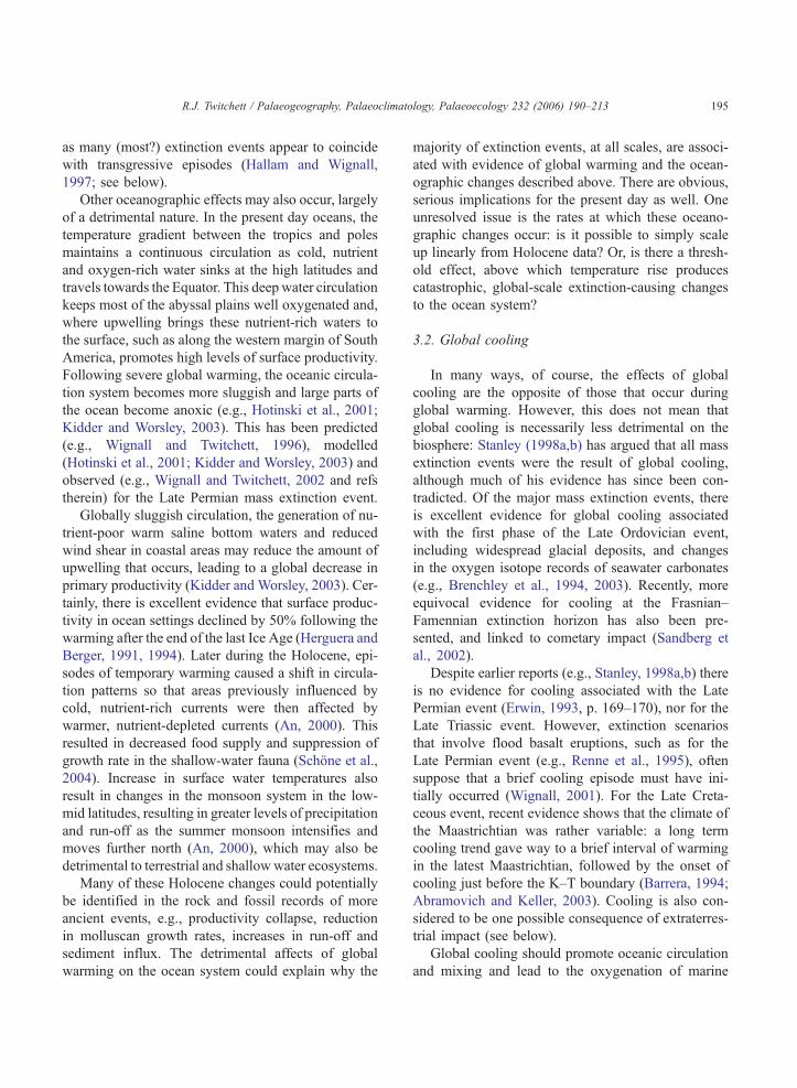
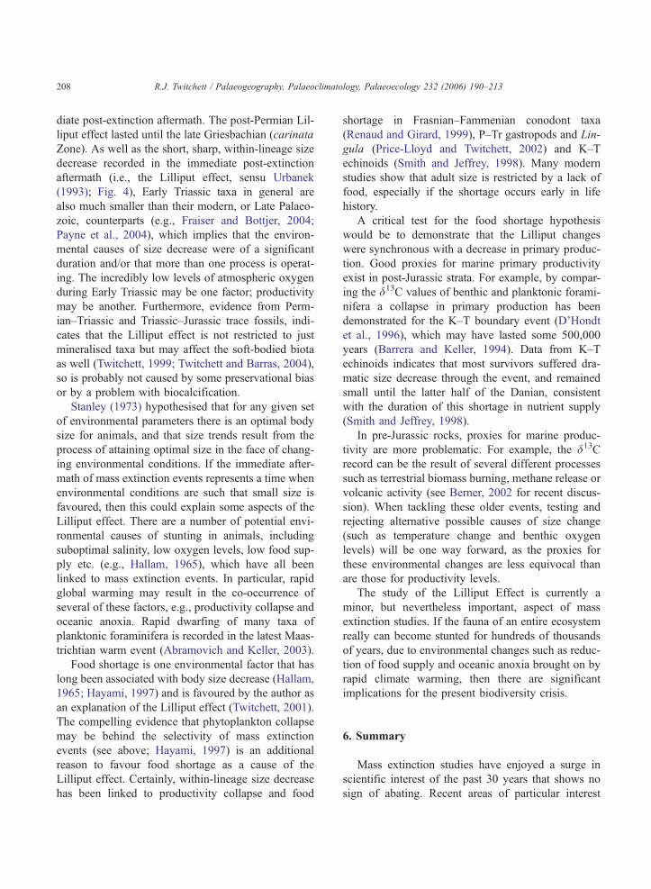
nitude. The model (Fig. 2) is based on the application

of theoretical concepts of survivorship to the fossil

record. In particular, a number of possible survival

mechanisms were proposed (see for example, Harries

et al., 1996), and taxa in the extinction aftermath were

interpreted as having survived by virtue of one or

other survival mechanism, based on characteristics

of their stratigraphic range (Fig. 2).

EX

TIN

CT

ION

INT

ER

VA

LB

AC

KG

RO

UN

DC

ON

DIT

ION

SS

UR

VIV

AL

RE

CO

VE

RY

RE

PO

PU

LAT

ION

IN

TE

RV

AL

A B C D

E

F

G H I

Fig. 2. The Kauffman–Erwin model of recovery after mass extinc-

tion events (modified from Kauffman and Erwin, 1995). A=pre-

adapted survivors; B=ecological generalists; C=disaster species;

D=opportunistic species; E=failed crisis progenitors; F=crisis pro-

genitors; G=stranded populations; H=short-term refugia species;

I= long-term refugia species. Grey shaded area represents refugia,

outside the normal geographic range of the refugia species. For

definitions of taxa see Kauffman and Harries (1996).

This over-emphasis on interpretations based on

literal reading of the stratigraphic ranges of fossil

taxa, has led to criticism of some aspects of the

model. For example, Lazarus taxa (those taxa that

temporarily disappear from the fossil record) are

termed instead bRefugia taxaQ, of which two types

(Short Term Refugia Species and Long Term Refugia

Species) have been identified (Kauffman and Harries,

1996). The key stratigraphic characteristic is a tem-

porary absence from the fossil record, during which

time the species in question emigrated to some un-

known refugium, outside of their normal geographical

range (Harries et al., 1996), before returning to help

seed the subsequent post-event radiation. This inter-

pretation of Lazarus taxa is easy to criticise on several

grounds, biological and geological, including the fact

that changes in facies or preservation potential is an

alternative, far more plausible, reason for temporary

absence from the fossil record (e.g., Erwin, 1996;

Twitchett, 2000). Biologically, it is highly unlikely

that species could successfully colonise a novel hab-

itat or region, just in time to escape the biotic crisis,

yet were unable to colonise that area prior to the event

(Wignall, 1994). More likely, shrinkage of the original

range to a core area would happen during the crisis,

with subsequent re-colonisation of the previous range

once conditions improve; a pattern observed in mod-

ern taxa (Twitchett, 2001, p. 347).

Regardless of these difficulties with the Kauffman

and Erwin (1995) and Kauffman and Harries (1996)

interpretations, several aspects of their model have

been incorporated into the study of post-extinction

recovery. One is the twofold division of the post-

extinction bRepopulation IntervalQ into an initial

bSurvival IntervalQ and a later bRecovery IntervalQ(Fig. 2). The boundary is marked by the onset of

significant post-extinction radiation, and comparing

the duration of Survival Intervals is one possible

method of comparing the rates of recovery after dif-

ferent events (e.g., Erwin, 1998, 2001). There is a

minor issue of nomenclature here: many authors pre-

fer to use the common term brecovery intervalQ whenreferring to the whole of the post-extinction aftermath,

rather than the Kauffman and Erwin term

brepopulation intervalQ.Additionally, terms like bDisaster speciesQ, or

bDisaster taxaQ have subsequently become common-

place in studies of mass extinction events. During

R.J. Twitchett / Palaeogeography, Palaeoclimatology, Palaeoecology 232 (2006) 190–213204

background times, disaster taxa (as defined) are geo-

graphically restricted, often to marginal, high stress

environments. This is supposedly due to their exclu-

sion from other (by inference, more bnormalQ) habitatsthrough competition from other organisms (Kauffman

and Harries, 1996, p. 20). In the immediate aftermath

of the extinction event (early Survival Interval), di-

saster species are briefly widespread and abundant,

with a larger geographic range that includes these

more bnormalQ habitats, before retreating into relative

obscurity once more. This post-extinction bloom of

disaster species is interpreted as being due to the

extinction of their competitors (i.e., relaxation of bi-

otic control), but, alternatively, could simply indicate

a temporary expansion, into these other environments,

of the deleterious environmental conditions to which

they are adapted (i.e., abiotic control).

In the aftermath of the Late Permian event, the

inarticulate brachiopod Lingula is interpreted as a

disaster taxon (e.g., Schubert and Bottjer, 1995; Rod-

land and Bottjer, 2001). Rare in pre-extinction shal-

low marine assemblages, Lingula often, though not

always, dominates assemblages in the immediate post-

extinction aftermath (specifically the first one or two

conodont zones of the Induan) and is globally wide-

spread in shallow subtidal environments (Rodland and

Bottjer, 2001). In the aftermath of the K–T event,

blooms of the small opportunistic disaster taxon

Guembelitria have been documented (Keller and

Pardo, in press). Similarly, post-extinction stromato-

lites, or other microbial structures, are typically inter-

preted as disaster dtaxaT, or ddisaster formsT (e.g.,

Schubert and Bottjer, 1992, 1995; Whalen et al.,

2002).

At the global, Phanerozoic-level scale, stromato-

lites seem an archetypal disaster ’taxon’, having

enjoyed former glory throughout the shallow subtidal

environments of the Proterozoic, before being restrict-

ed to marginal, hypersaline settings in the Phanerozo-

ic. Only after the mass extinction events of the

Phanerozoic, primarily the Late Permian (e.g., Schu-

bert and Bottjer, 1992) but also the Late Devonian

(Whalen et al., 2002), were they able to colonise other

subtidal settings and become, temporarily, common in

the fossil record once more. This was made possible

by the widespread extinction of the metazoan infauna

and/or continuation of deleterious environmental con-

ditions unsuitable for burrowing benthos, which led to

the return of Proterozoic-like substrate conditions

(Pruss et al., 2004).

However, there are problems with this scenario.

Firstly, regarding the Late Devonian event, Shen and

Webb (2004) have recently cast doubt on the inter-

pretation of Whalen et al. (2002) on Famennian

stromatolite reefs as disaster forms. They note that

salinity, nutrient availability and sediment influx may

be the primary controls on stromatolite distribution,

and that stromatolite reefs and other microbial build-

ups are common throughout the Late Devonian (be-

fore, during and after the extinction crisis) and may

be associated with a diverse fauna (Shen and Webb,

2004). Secondly, according to the Kauffman–Erwin

model (Fig. 2), the definition of disaster taxa is that

they only bloom in the very earliest part of the

Survival Interval. In the aftermath of the Late Perm-

ian event, stromatolites and other microbial struc-

tures, such as wrinkle structures (Pruss et al.,

2004), are encountered at various horizons and in

various depositional settings throughout the Early

Triassic, including the late Olenekian (Spathian)

where there is unequivocal evidence of increasing

diversity and recovery.

Part of the reason is probably that some of these

records are, in fact, from marginal, salinity-stressed

environments and not bnormalQ subtidal settings.

Many of the Olenekian examples of microbial struc-

tures derive from the Moenkopi Formation of SE

Nevada, USA (Schubert and Bottjer, 1992, 1995;

Pruss et al., 2004), which is a very marginal setting.

Stromatolites are absent from coeval strata in northern

Nevada that were deposited in more open marine

conditions (pers. observ.). The high abundance of

microbial wrinkle structures in the Campil Member

of the Werfen Formation (northern Italy) (Pruss et al.,

2004) is almost certainly due to the brackish deposi-

tional environment (e.g., Twitchett, 1999). Wrinkle

marks are very common in such brackish water,

tide-influenced facies throughout the Phanerozoic

(e.g., Mangano and Buatois, 2004) and no special

evolutionary/environmental argument is necessary to

explain their occurrence in equivalent facies of Early

Triassic age. Indeed, the tidal flat facies of the Car-

boniferous Stull Shale of Kansas (Mangano and Bua-

tois, 2004, Fig. 4b, p. 163), which contains abundant

wrinkle structures, is identical to facies of the upper

Moenkopi Formation of southern Nevada (Pruss et al.,

R.J. Twitchett / Palaeogeography, Palaeoclimatology, Palaeoecology 232 (2006) 190–213 205

2004, Fig. 3d, p. 363); only the interpretations are

different.

Even microbialites of the immediate post-Permian

aftermath are not universally considered to represent

disaster forms (Kershaw et al., 2002) as other abiotic

factors apparently controlled their distribution (cf.

Shen and Webb, 2004). These conflicts demonstrate

the potential dangers of letting a model control one’s

interpretations of the fossil record, without due con-

sideration of possible alternatives. Such bhypothesis-driven interpretationsQ (Stinnesbeck et al., 1994) are,

unfortunately, rather common in the study of extinc-

tion events. Clearly, more detailed work is needed to

determine the factors controlling the distribution of

so-called disaster taxa.

5.2.2. A new recovery model?

More recently, efforts have got underway to con-

struct an alternative method of describing marine

benthic recovery based on empirical data from the

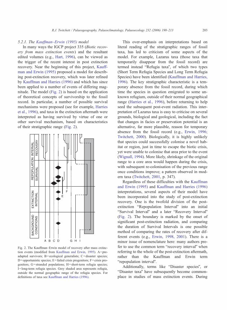
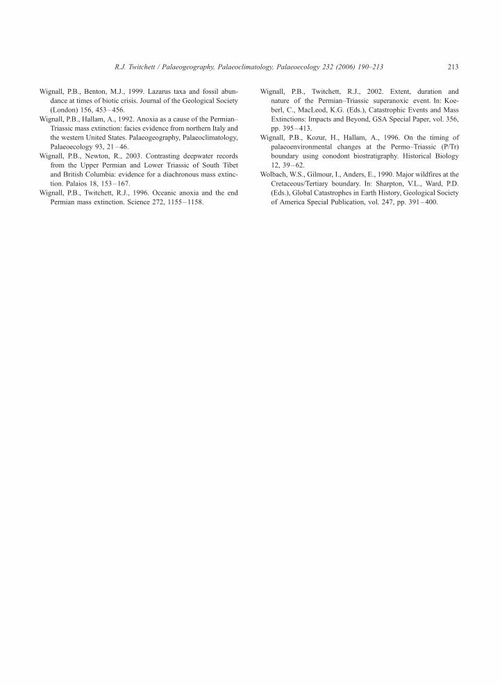
fossil record (Twitchett et al., 2004). The currently

proposed ordinal scheme comprises four Recovery

Stages, from the initial post-extinction aftermath to

TIE

RIN

G

LEV

ELS

RECOVERY

1 2

ICH

NO

LOG

Y

- simple fodinichnia- diameters < 5mm- very low diversity- e.g. Planolites

- vertical domichnia- e.g. Arenicolites, Diplocraterion- small diameters

SH

ELL

YFA

UN

A - low diversity- high dominance- small size

epifauna

infauna

Fig. 3. Four stage palaeoecological model for recovery of benthic marin

observations of the fossil record of Permian–Triassic shallow shelf setting

the final recovery of the benthic fauna (Fig. 3) and is

based on observation of fossil assemblages from

Permian–Triassic shallow shelf environments. The

broad aim of devising such a model is to allow

comparison of the rates of recovery between different

regions or localities in the aftermath of a single event,

or between different events. The model incorporates

data on trace fossils, which are the only records of

responses of the soft-bodied biota to extinction events

(Twitchett and Barras, 2004), as well as body fossils,

and thus could potentially be used to compare ancient

events with modern, smaller scale defaunation events

and experimental work.

Several key palaeoecological criteria have been

found to be most useful in the discrimination of the

recovery stages: (1) tiering levels, (2) the presence/

absence of key ichnotaxa, (3) body (or burrow) size

and (4) dominance and evenness of shelly assem-

blages. Diversity also changes through the recovery

interval, of course, but not necessarily in a predictable

way. For example, the sudden appearance of many

opportunists in the aftermath of an event may lead to a

peak in local (alpha) diversity prior to final recovery

STAGES

3 4

- increased diversity- Rhizocorallium- rare Thalassinoides- diameters < 20mm

- high diversity- high complexity- common, large Thalassinoides- diameters > 20mm

- high diversity- low dominance- large size

e ecosystems in the aftermath of biotic crises, based on empirical

s (see also Twitchett et al., 2004). See text for further details.

R.J. Twitchett / Palaeogeography, Palaeoclimatology, Palaeoecology 232 (2006) 190–213206

and has been recorded in both modern (Lu and Wu,

2000) and ancient (Looy et al., 2001) events. In

addition, measured diversity maybe affected by fac-

tors such as preservation, taphonomy and the scale of

the study (e.g., field observations, study of museum

specimens, thin section analyses etc.).

Tiering (sensu Ausich and Bottjer, 1982) is a very

useful measure of ecological recovery (e.g., Twitchett,

1999). Tiering describes the vertical stratification of

marine suspension feeders above and below the level

of the substrate. The epifaunal and infaunal tiers

appear to be decoupled, and tiering levels have

changed through time (Ausich and Bottjer, 1982;

Bottjer and Ausich, 1986). Recently, it has been rea-

lised that mass extinction events cause a temporary,

dramatic reduction in tiering levels (e.g., Bottjer et al.,

1996; Twitchett and Barras, 2004), and so the recov-

ery of tiering back to pre-event levels can be used to

assess benthic recovery (Twitchett et al., 2004; Fig. 3).

In the immediate aftermath (Recovery Stage 1) epi-

faunal and infaunal tiering is reduced to a bare min-

imum. Next, infaunal tiering begins to recover

(Recovery Stage 2), followed by epifaunal tiering

(Recovery Stage 3). Finally, pre-extinction levels of

tiering are attained (Recovery Stage 4). Infaunal tier-

ing can be measured directly from the depth of bio-

turbation (e.g., Twitchett and Barras, 2004), or

inferred from e.g., the morphology of the shelly,

infaunal mollusca. Epifaunal tiering is measured

from the shelly remains (e.g., articulated crinoids).

In the absence of articulated material, the presence

of a high tier can still be inferred from the presence of

e.g., disarticulated crinoid ossicles. Such ossicles have

a very high preservation potential, and so although

absence may be due to shell bed taphonomy, this bias

is considered to be minimal.

Recent work on the post-extinction trace fossil

records of the early Triassic and Early Jurassic (e.g.,

Twitchett and Wignall, 1996; Twitchett, 1999; Twitch-

ett and Barras, 2004) have shown that there is a

stepwise reappearance in certain ichnotaxa during

the post-extinction recovery. At first, Twitchett

(1999) supposed that the re-appearances were globally

synchronous. However, this is not the case, and al-

though the sequence of trace fossil recovery remains

similar worldwide, at least after the Late Permian and

Late Triassic events (Twitchett and Barras, 2004), the

timing of reappearance of specific ichnotaxa may be

globally diachronous. Thus, trace fossils can be used

as a measure of relative recovery rates. The immediate

extinction aftermath (Recovery Stage 1) is charac-

terised by the presence of rare, small, simple fodinich-

nia (e.g., Planolites) of deposite feeding animals and

an absence of the vertical domichnia of suspension

feeders. Subsequently, these domichnia (e.g., Areni-

colites and Diplocraterion) appear in Recovery Stage

2, and are themselves followed by ichnotaxa that may

be attributable to burrowing crustaceans, such as Rhi-

zocorallium and, sometimes, small Thalassinoides

(Recovery Stage 3). A return to pre-extinction ichno-

diversity, burrow size and amount of bioturbation

characterises the final stage of recovery. The reappear-

ance of common, large (N20 mm) diameter Thalassi-

noides and/or Rhizocorallium burrows are considered

particularly indicative of the final stage of benthic

recovery (Twitchett et al., 2004).

The combination of ichnology and tiering are

viewed as particularly powerful tools for documenting

benthic recovery in marine shelf settings, and can be

easily applied in the field. Other useful measures

include organism size (or burrow diameter), which

is typically very low in the extinction aftermath and

increases again through the post-extinction recovery.

Changes in tiering and organism size hint at profound

changes in the biomass of marine ecosystems through

these events. In addition, ecological parameters such

as the dominance and evenness of fossil assemblages

also provide a measure of recovery, although care is

required in their application, as they are particularly

sensitive to changes in taphonomy and preservation.

Typically, the immediate post-extinction aftermath

(Recovery Stage 1) is characterised by high domi-

nance (often also high abundance) assemblages

(e.g., Schubert and Bottjer, 1995; Twitchett, 1999;

Twitchett et al., 2004), whereas the final stage of

recovery is characterised by a return to more ‘even’

communities. When the changeover occurs is not very

clear, although from a theoretical point of view it

should be at the boundary between the Survival and

Recovery Intervals of Kauffman and Harries (1996).

As this model is applied more widely, it will no

doubt be refined and probably superseded by better

methods. As Erwin (1998, 2001) has noted, quantify-

ing biotic recovery is certainly not easy. It is, however,

of prime importance as we seek to more fully under-

stand the way in which the global biosphere has

parvus isarcica carinata

GriesbachianLate

Permian

0

10

20

30

40

50Size (mm)

Fig. 4. Temporary size decrease (the Lilliput effect) in benthic marine

invertebrates in the aftermath (Griesbachian substage) of the Perm

ian–Triassic mass extinction event. Black square=Bellerophon

(n =42); grey circle=Lingula (n =195); black diamond=Claraia

(n =721); grey triangle=Unionites (n =258). Symbols show mean

size, horizontal lines indicate maximum and minimum recorded

sizes. Size calculated as the geometric mean of length and height

All within-taxon size changes are significant at the 5% level (Kol

mogorov–Smirnov test). Data collected in the field from localities in

northern Italy (Bellerophon and Werfen Formations). The Griesba

chian is divided into three conodont zones: parvus, isarcica and

carinata. Arrow indicates approximate position of extinction event

Data modified from Price-Lloyd and Twitchett (2002).

R.J. Twitchett / Palaeogeography, Palaeoclimatology, Palaeoecology 232 (2006) 190–213 207

responded to extinction events in the past and how

different events compare. Successful management of

the present-day biodiversity crisis and its aftermath

may depend upon such studies.

5.3. Size change (the Lilliput Effect)

Adam Urbanek (1993) described a bpost-eventsyndromeQ that affected Silurian graptolites, and is

very applicable to the aftermath of mass extinction

events as well. One aspect of this model that is

particularly important is his bLilliput effectQ. This

term refers to the pattern of size change through

extinction events, specifically the temporary appear-

ance of organisms with suboptimal body size (i.e.,

dwarfism or stunting) in the immediate aftermath.

Body size is a key morphological variable, with impli-

cations for many aspects of an animal’s biology,

behaviour and ecology, and so understanding the

Lilliput effect may be crucial in understanding the

nature of ecological, environmental and biological

change during past biotic crises.

The study of Urbanek (1993) documented a size

decrease in several taxa of Silurian graptolites, all of

which were holdover or survivor taxa of (relatively)

minor biotic crises. In the subsequent decade, the

Lilliput effect has been recognised in the aftermath

of the five mass extinction events and has been docu-

mented in a wide variety of animal groups (Twitchett,

2001 and refs. therein). It appears to be a factor that is

common to all known extinction crises. Do animals

respond in a similar (and therefore predictable) way to

all biotic crises regardless of scale and forcing mech-

anism? If so, then this has important implications for

our understanding of the response of organisms to

ecological disturbance at both global and local scale,

and may even allow us to predict the future response

of the biosphere to present-day environmental change.

Alternatively, does this commonality imply that a

single proximate cause links all major extinction

events of the past?

What are the possible causes of size decrease fol-

lowing extinction events? The simplest explanation is

to invoke size selection during the extinction event

itself, which causes the demise of large K-selected

taxa and heralds their replacement by small, r-selected

opportunists. While post-extinction size increase has

been explained in terms of changes in life-history

strategy (e.g., Hallam, 1975), to date no study has

demonstrated that extinctions are size selective

(Jablonski, 1996; discussion above), although selec-

tion against large body size was invoked as an expla-

nation for size changes in K–T and P–Tr bivalves

(Hayami, 1997). At the K/T boundary event, while

all of the large, specialist (K-selected) planktonic

foraminifera disappeared, so did all the small trochos-

piral ecological generalist taxa (except the hedbergel-

lids, which became extinct in the early Danian)

(Keller, 2003).

The Lilliput effect of Urbanek (1993) explicitly

describes temporary, within-lineage size decrease of

the surviving organisms. Data collected by the author

from a number of Early Triassic assemblages world-

wide show that not only are surviving taxa smaller

than expected, but taxa which originate in the imme-

diate aftermath of the Late Permian extinction crisis

are also significantly smaller than later forms (Fig. 4).

Therefore, the Lilliput effect is not restricted to just

the holdover taxa (cf. Urbanek, 1993), and may be

caused by the nature of the environment in the imme-

-

.

-

-

.

R.J. Twitchett / Palaeogeography, Palaeoclimatology, Palaeoecology 232 (2006) 190–213208

diate post-extinction aftermath. The post-Permian Lil-

liput effect lasted until the late Griesbachian (carinata

Zone). As well as the short, sharp, within-lineage size

decrease recorded in the immediate post-extinction

aftermath (i.e., the Lilliput effect, sensu Urbanek

(1993); Fig. 4), Early Triassic taxa in general are

also much smaller than their modern, or Late Palaeo-

zoic, counterparts (e.g., Fraiser and Bottjer, 2004;

Payne et al., 2004), which implies that the environ-

mental causes of size decrease were of a significant

duration and/or that more than one process is operat-

ing. The incredibly low levels of atmospheric oxygen

during Early Triassic may be one factor; productivity

may be another. Furthermore, evidence from Perm-

ian–Triassic and Triassic–Jurassic trace fossils, indi-

cates that the Lilliput effect is not restricted to just

mineralised taxa but may affect the soft-bodied biota

as well (Twitchett, 1999; Twitchett and Barras, 2004),

so is probably not caused by some preservational bias

or by a problem with biocalcification.

Stanley (1973) hypothesised that for any given set

of environmental parameters there is an optimal body

size for animals, and that size trends result from the

process of attaining optimal size in the face of chang-

ing environmental conditions. If the immediate after-

math of mass extinction events represents a time when

environmental conditions are such that small size is

favoured, then this could explain some aspects of the

Lilliput effect. There are a number of potential envi-

ronmental causes of stunting in animals, including

suboptimal salinity, low oxygen levels, low food sup-

ply etc. (e.g., Hallam, 1965), which have all been

linked to mass extinction events. In particular, rapid

global warming may result in the co-occurrence of

several of these factors, e.g., productivity collapse and

oceanic anoxia. Rapid dwarfing of many taxa of

planktonic foraminifera is recorded in the latest Maas-

trichtian warm event (Abramovich and Keller, 2003).

Food shortage is one environmental factor that has

long been associated with body size decrease (Hallam,

1965; Hayami, 1997) and is favoured by the author as

an explanation of the Lilliput effect (Twitchett, 2001).

The compelling evidence that phytoplankton collapse

may be behind the selectivity of mass extinction

events (see above; Hayami, 1997) is an additional

reason to favour food shortage as a cause of the

Lilliput effect. Certainly, within-lineage size decrease

has been linked to productivity collapse and food

shortage in Frasnian–Fammenian conodont taxa

(Renaud and Girard, 1999), P–Tr gastropods and Lin-

gula (Price-Lloyd and Twitchett, 2002) and K–T

echinoids (Smith and Jeffrey, 1998). Many modern

studies show that adult size is restricted by a lack of

food, especially if the shortage occurs early in life

history.

A critical test for the food shortage hypothesis

would be to demonstrate that the Lilliput changes

were synchronous with a decrease in primary produc-

tion. Good proxies for marine primary productivity

exist in post-Jurassic strata. For example, by compar-

ing the d13C values of benthic and planktonic forami-

nifera a collapse in primary production has been

demonstrated for the K–T boundary event (D’Hondt

et al., 1996), which may have lasted some 500,000

years (Barrera and Keller, 1994). Data from K–T

echinoids indicates that most survivors suffered dra-

matic size decrease through the event, and remained

small until the latter half of the Danian, consistent

with the duration of this shortage in nutrient supply

(Smith and Jeffrey, 1998).

In pre-Jurassic rocks, proxies for marine produc-

tivity are more problematic. For example, the d13C

record can be the result of several different processes

such as terrestrial biomass burning, methane release or

volcanic activity (see Berner, 2002 for recent discus-

sion). When tackling these older events, testing and

rejecting alternative possible causes of size change

(such as temperature change and benthic oxygen

levels) will be one way forward, as the proxies for

these environmental changes are less equivocal than

are those for productivity levels.

The study of the Lilliput Effect is currently a

minor, but nevertheless important, aspect of mass

extinction studies. If the fauna of an entire ecosystem

really can become stunted for hundreds of thousands

of years, due to environmental changes such as reduc-

tion of food supply and oceanic anoxia brought on by

rapid climate warming, then there are significant

implications for the present biodiversity crisis.

6. Summary

Mass extinction studies have enjoyed a surge in

scientific interest of the past 30 years that shows no

sign of abating. Recent areas of particular interest

R.J. Twitchett / Palaeogeography, Palaeoclimatology, Palaeoecology 232 (2006) 190–213 209

include the palaeoecological study of biotic crises, and

analyses of patterns of post-extinction recovery. There

is good evidence of rapid climate change affecting all

of the major extinction events, while the ability of

extraterrestrial impact to cause extinction remains

debatable. There is growing evidence that food short-

age and suppression of primary productivity, lasting

several hundred thousand years, may be a proximate

cause of many past extinction events. Selective ex-

tinction of suspension feeders and the prevalence of

dwarfed organisms in the aftermath are palaeoecolo-

gical consequences of these changes. The association

with rapid global warming shows that study of mass

extinction events is not just an esoteric intellectual

exercise, but may have implications for the present

day.

Acknowledgements

This publication was written during tenureship of a

Research Fellowship from the Japan Society for the

Promotion of Science, at the University of Tokyo,

Japan. I thank D. Erwin and an anonymous reviewer

for pointing out the errors and omissions in an earlier

draft; any mistakes that remain are my own.

References

Abramovich, S., Keller, G., 2003. Planktonic foraminiferal response

to the latest Maastrichtian abrupt warm event: a case study from

South Atlantic DSDP Site 525A. Marine Micropalaeontology

48, 225–249.

Allison, P.A., Briggs, D.E.G., 1993. Paleolatitudinal sampling bias,

Phanerozoic species diversity, and the end-Permian extinction.

Geology 21, 65–68.

Alvarez, W., 1997. T. rex and the Crater of Doom. Penguin,

Princeton, New Jersey.

Alvarez, L.W., Alvarez, W., Asaro, F., Michel, H.V., 1980. Extra-

terrestrial causes of the Cretaceous–Tertiary extinction. Science

208, 1095–1108.

An, Z., 2000. The history and variability of the East Asian paleo-

monsoon climate. Quaternary Science Reviews 19, 171–187.

Ausich, W.I., Bottjer, D.J., 1982. Tiering in suspension feeding

communities on soft substrata throughout the Phanerozoic. Sci-

ence 216, 173–174.

Barrera, E., 1994. Global environmental changes preceding the

Cretaceous–Tertiary boundary: Early–Late Maastrichtian transi-

tion. Geology 22, 877–880.

Barrera, E., Keller, G., 1994. Productivity across the Cretaceous–

Tertiary boundary in high latitudes. Geological Society of Amer-

ica Bulletin 106, 1254–1266.

Becker, L., Poreda, R.J., Basu, A.R., Pope, K.O., Harrison, T.M.,

Nicholson, C., Iasky, R., 2004. Bedout: a possible end-Permian

impact crater offshore of northwestern Australia. Science 304,

1469–1476.

Belcher, C.M., Collinson, M.E., Sweet, A.R., Hildebrand, A.R.,

Scott, A.C., 2003. Fireball passes and nothing burns—the role

of thermal radiation in the Cretaceous–Tertiary event: evidence

from the charcoal record of North America. Geology 31,

1061–1064.

Benton, M.J. (Ed.), 1993. The Fossil Record 2. Chapman and Hall,

London.

Benton, M.J., 1995. Diversification and extinction in the history of

life. Science 268, 52–58.

Benton, M.J., 2003. When Life Nearly Died: the Greatest Mass

Extinction of All Time. Thames and Hudson, London. 336 pp.

Benton, M.J., Twitchett, R.J., 2003. How to kill (almost) all life: the

end-Permian extinction event. Trends in Ecology and Evolution

18, 358–365.

Berner, R.A., 2002. Examination of hypotheses for the Permo–

Triassic boundary extinction by carbon cycle modelling. Pro-

ceedings of the National Academy of Sciences 99, 4172–4177.

Bottjer, D.J., Ausich, W.I., 1986. Phanerozoic development of tier-

ing in soft substrata suspension-feeding communities. Paleobi-

ology 12, 400–420.

Bottjer, D.J., Schubert, J.K., Droser, M.L., 1996. Comparative

evolutionary palaeoecology: assessing the changing ecology of

the past. In: Hart, M.B. (Ed.), Biotic Recovery from Mass

Extinction Events, Geological Society, London, Special Publi-

cations, vol. 102, pp. 1–13.

Bourgeois, J., Hansen, T.A., Wiberg, P.L., Kauffman, E.F., 1988. A

tsunami deposit at the Cretaceous–Tertiary boundary in Texas.

Science 241, 567–570.

Brenchley, P.J., Marshall, J.D., Carden, G.A.F., Roberston, D.B.R.,

Long, G.D.F., Meidla, T., Hints, L., Andreson, T.F., 1994.

Bathymetric and isotopic evidence for a short-lived Late Ordo-

vician glaciation in a greenhouse period. Geology 22, 295–298.

Brenchley, P.J., Carden, G.A., Hints, L., Kaljo, D., Marshall, J.D.,

Martana, T., Meidla, T., Nolvak, J., 2003. High-resolution stable

isotope stratigraphy of Upper Ordovician sequences: constraints

on the timing of bioevents and environmental changes associ-

ated with mass extinction and glaciation. GSA Bulletin 115,

89–104.

Briggs, D.E.G., Gall, J.-C., 1990. The continuum in soft-bodied

biotas from transitional environments: a quantitative comparison

of Triassic and Carboniferous Konservat–Lagerstatten. Paleobi-

ology 16, 204–218.

Brookfield, M.E., Twitchett, R.J., Goodings, C., 2003. Palaeoenvir-

onments of the Permian–Triassic transition sections in Kashmir,

India. Palaeogeography, Palaeoclimatology, Palaeoecology 198,

353–371.

Covey, C., Ghan, S.J., Walton, J.J., Weissman, P.R., 1990. Global

environmental effects of impact-generated aerosols: results from

a general circulation model. In: Sharpton, V.L., Ward, P.D.

R.J. Twitchett / Palaeogeography, Palaeoclimatology, Palaeoecology 232 (2006) 190–213210

(Eds.), Global Catastrophes in Earth History, Geological Society

of America, Special Publication, vol. 247, pp. 263–270.

Cuny, G., 1995. French vertebrate faunas and the Triassic–Jurassic

boundary. Palaeogeography, Palaeoclimatology, Palaeoecology

119, 343–358.

D’Hondt, S., Herbert, T.D., King, J., Gibson, C., 1996. Planktic

foraminifera, asteroids, and marine production: death and recov-

ery at the Cretaceous–Tertiary boundary. In: Ryder, G., Fas-

tovsky, D., Gartner, S. (Eds.), The Cretaceous–Tertiary Event

and Other Catastrophes in Earth History, Geological Society of

America Special Paper, vol. 307, pp. 303–317.

Droser, M.L., Bottjer, D.J., Sheehan, P.M., McGhee, G.R., 2000.

Decoupling of taxonomic and ecologic severity of Phanerozoic

mass extinctions. Geology 28, 675–678.

Ekdale, A.A., Stinnesbeck, W., 1998. Trace fossils in Cretaceous–

Tertiary (KT) boundary beds in northeastern Mexico: implica-

tions for sedimentation during the KT boundary event. Palaios

13, 593–602.

Erwin, D.H., 1989. Regional paleoecology of Permian gastropod

genera, southwestern United States, and the end-Permian mass

extinction. Palaios 4, 424–438.

Erwin, D.H., 1993. The Great Paleozoic Crisis: Life and Death in

the Permian. Columbia University Press, New York. 327 pp.

Erwin, D.H., 1996. Understanding biotic recoveries: extinction,

survival, and preservation during the end-Permian Mass Ex-

tinction. In: Jablonski, D., Erwin, D.H., Lipps, J.H. (Eds.),

Evolutionary Paleobiology. University of Chicago Press, Chi-

cago, pp. 398–418.

Erwin, D.H., 1998. The end and the beginning: recoveries from mass

extinctions. Trends in Ecology and Evolution 13, 344–349.

Erwin, D.H., 2001. Lessons from the past: biotic recoveries from

mass extinctions. Proceedings of the National Academy of

Sciences 98, 5399–5403.

Finney, S.C., Berry, W.B.N, Cooper, J.D., Ripperdan, R.L., Sweet,

W.C., Jacobson, S.R., Soufiane, A., Achab, A., Noble, P.J.,

1999. Late Ordovician mass extinction: a new perspective

from stratigraphic sections in central Nevada. Geology 27,

215–218.

Foster, C.B., Logan, G.A., Summons, R.E., Gorter, J.D., Edwards,

D.S., 1997. Carbon isotopes, kerogen types and the Permian–

Triassic boundary in Australia: implications for exploration.

APPEA Journal 37, 472–489.

Fraiser, M.L., Bottjer, D.J., 2004. The non-actualistic Early Triassic

gastropod fauna: a case study of the Lower Triassic Sinbad

Limestone Member. Palaios 19, 259–275.

Grice, K., Cao, C., Love, G.D., Bottcher, M.E., Twitchett, R.J.,

Grosjean, E., Summons, R.E., Turgeon, S.C., William Dunning,

W., Jin, Y., 2005. Photic zone euxinia during the Permian–

Triassic superanoxic event. Science 307, 706–709.

Hallam, A., 1965. Environmental causes of stunting in living

and fossil marine benthonic invertebrates. Palaeontology 8,

132–155.

Hallam, A., 1975. Evolutionary size increase and longevity in

Jurassic bivalves and ammonites. Nature 258, 493–496.

Hallam, A., 2002. How catastrophic was the end-Triassic mass

extinction? Lethaia 35, 147–157.

Hallam, A., Wignall, P.B., 1997. Mass Extinctions and Their Af-

termath. Oxford University Press, New York. 320 pp.

Hallam, A., Wignall, P.B., 1999. Mass extinctions and sea-level

changes. Earth Science Reviews 48, 217–250.

Hallam, A., Wignall, P.B., 2000. Facies changes across the Triassic–

Jurassic boundary in Nevada, USA. Journal of the Geological

Society (London) 157, 49–54.

Hansen, T.A., Kelley, P.H., Haasl, D.M., 2004. Paleoecological

pattern in molluscan extinctions and recoveries: comparison of

the Cretaceous–Paleogene and Eocene–Oligocene extinctions in

North America. Palaeogeography, Palaeoclimatology, Palaeoe-

cology 214, 233–242.

Harper, D.E., Salzer, R.R., Case, R.J., 1981. The occurrence of

hypoxic bottom water off the Upper Texas coast and its

effect on the benthic biota. Contributions to Marine Science

24, 53–79.

Harries, P.J., Kauffman, E.G., Hansen, T.A., 1996. Models for biotic

survival following mass extinction. In: Hart, M.B. (Ed.), Biotic

Recovery from Mass Extinction Events, Geological Society,

London, Special Publications, vol. 102, pp. 41–60.

Hart, M.B. (Ed.), 1996. Biotic Recovery from Mass Extinction

Events, Geological Society of London Special Publication,

vol. 102. The Geological Society, London. 392 pp.

Hayami, I., 1997. Size changes of bivalves and a hypothesis

about the cause of mass extinction. Fossils 62, 24–36 (in

Japanese).

Herguera, J.C., Berger, W.H., 1991. Paleoproductivity from benthic

foraminiferal abundance—glacial to postglacial change in the

western Equatorial Pacific. Geology 19, 1173–1176.

Herguera, J.C., Berger, W.H., 1994. Glacial to post-glacial drop in

productivity in the western Equatorial Pacific—mixing rate vs

nutrient concentrations. Geology 22, 629–632.

Hildebrand, A.R., Penfield, G.T., Kring, D.A., Pilkington, M.,

Camargo, Z.A., 1991. Chicxulub crater: a possible Cretaceous/

Tertiary boundary impact crater in the Yucatan Peninsula. Ge-

ology 19, 867–871.

Holland, S.M., 1995. The stratigraphic distribution of fossils. Pa-

leobiology 21, 92–109.

Hotinski, R.M., Bice, K.L., Kump, L.R., Najjar, R.G., Arthur, M.A.,

2001. Ocean stagnation and end-Permian anoxia. Geology 29,

7–10.

Jablonski, D., 1986. Background and mass extinctions: the alter-

ation of macroevolutionary regimes. Science 231, 129–133.

Jablonski, D., 1996. Body size and macroevolution. In: Jablonski,

D., Erwin, D.H., Lipps, J.H. (Eds.), Evolutionary Paleobiology.

Chicago University Press, Chicago, pp. 256–289.

Jablonski, D., Raup, D.M., 1995. Selectivity of end-Cretaceous

marine bivalve extinctions. Science 268, 389–391.

Jeffery, C.H., 2001. Heart urchins at the Cretaceous/Tertiary bound-

ary: a tale of two clades. Paleobiology 27, 140–158.

Kauffman, E.G., Erwin, D.H., 1995. Surviving mass extinctions.

Geotimes 14, 14–17.

Kauffman, E.G., Harries, P.J., 1996. The importance of crisis pro-

genitors in recovery from mass extinction. In: Hart, M.B. (Ed.),

Biotic Recovery from Mass Extinction Events, Geological So-

ciety, London, Special Publications, vol. 102, pp. 15–39.

R.J. Twitchett / Palaeogeography, Palaeoclimatology, Palaeoecology 232 (2006) 190–213 211

Keller, G., 2003. Biotic effects of impacts and volcanism. Earth and

Planetary Science Letters 215, 249–264.

Keller, G., Pardo, A., 2004. Disaster opportunists Guembelitrinidae:

index for environmental catastrophes. Marine Micropalaeonto-

logy 53, 83–116.

Keller, G., Adatte, T., Stinnesbeck, W., Rebolledo-Vieyra, M.,

Fucugauchi, J.U., Kramar, U., Stuben, D., 2004. Chicxulub

impact predates the K–T boundary mass extinction. PNAS

101, 3753–3758.

Kershaw, S., Guo, L., Swift, A., Fan, J.S., 2002. Microbialites in the

P–Tr boundary interval in Central China: structure, age and

distribution. Facies 47, 83–89.

Kidder, D.L., Worsley, D.R., 2003. Causes and consequences of ex-

treme Permo–Triassic warming to globally equable climate and

relation to thePermo–Triassic extinction and recovery. Palaeogeo-

graphy, Palaeoclimatology, Palaeoecology 203, 207–237.

Krull, E.S., Retallack, G.J., 2000. d13C depth profiles from paleo-

sols across the Permian–Triassic boundary: evidence for meth-

ane release. GSA Bulletin 112, 1459–1472.

Kump, L.R., 1991. Interpreting carbon-isotope excursions: Strange-

love oceans. Geology 19, 299–302.

Looy, C.V., Twitchett, R.J., Dilcher, D.L., Konijnenburg-Van Cit-

tert, J.H.A., Visscher, H., 2001. Life in the end-Permian dead

zone. Proceedings of the National Academy of Sciences 98,

7879–7883.

Lu, L., Wu, R.S.S., 2000. An experimental study on recolonization

and succession of marine macrobenthos in defaunated sediment.

Marine Biology 136, 291–302.

Luder, T., Benz, W., Stocker, T.F., 2002. Modeling long-term

climatic effects of impacts: first results. In: Koeberl, C.,

MacLeod, K.G. (Eds.), Catastrophic Events and Mass Extinc-

tions: Impacts and Beyond, Geological Society of America,

Special Paper, vol. 356, pp. 717–729.

MacLeod, N.M., 2004. The extinction of all life and the sublime

attraction of neocatastrophism. Palaeontology Newsletter 54,

49–64.

Mangano, M.G., Buatois, L.A., 2004. Ichnology of Carboniferous

tide-influenced environments and tidal flat variability in the North

American Midcontinent. In: McIlroy, D. (Ed.), The Application

of Ichnology to Palaeoenvironmental and Stratigraphic Analy-

sis, Geological Society, London, Special Publications, vol. 228,

pp. 157–178.

McElwain, J.C., Beerling, D.J., Woodward, F.I., 1999. Fossil plants

and global warming at the Triassic–Jurassic boundary. Science

285, 1386–1390.

McGhee, G.R., 1996. The Late Devonian Mass Extinction: the

Frasnian/Famennian Crisis. Columbia University Press, New

York. 303 pp.

McGhee, G.R., Sheehan, P.M., Bottjer, D.J., Droser, M.L., 2004.

Ecological ranking of Phanerozoic biodiversity crises: ecologi-

cal and taxonomic severities are decoupled. Palaeogeography,

Palaeoclimatology, Palaeoecology 211, 289–297.

McLaren, D.J., 1970. Presidential address: time, life and bound-

aries. Journal of Paleontology 44, 801–815.

Melosh, H.J., Schneider, N.M., Zahnle, K.J., Latham, D., 1990.

Ignition of global wildfires at the Cretaceous/Tertiary boundary.

Nature 343, 251–254.

Mii, H.S., Grossman, E.L., Yancey, T.E., 1997. Stable carbon and

oxygen isotopic shifts in Permian seas of West Spitsbergen:

global change or diagenetic artifact? Geology 25, 227–230.

Newell, N.D., 1952. Periodicity in invertebrate evolution. Journal of

Paleontology 26, 371–385.

Newell, N.D., 1962. Paleontological gaps and geochronology. Jour-

nal of Paleontology 36, 592–610.

Patterson, C., Smith, A.B., 1987. Is the periodicity of extinctions a

taxonomic artefact? Nature 330, 248–251.

Paul, C.R.C., Donovan, S.K., 1998. An overview of the complete-

ness of the fossil record. In: Donovan, S.K., Paul, C.R.C. (Eds.),

The Adequacy of the Fossil Record. John Wiley and Sons,

Chichester, pp. 111–132.

Payne, J.L., Lehrmann, D.J., Wei, J., Orchard, M.J., Schrag, D.P.,

Knoll, A.H., 2004. Large perturbations of the carbon cycle

during recovery from the end-Permian extinction. Science

305, 506–509.

Phillips, J., 1860. Life on Earth. Its Origin and Succession. Mac-

Millan, Cambridge.

Pollack, J.B., Toon, O.B., Ackerman, T.P., McKay, C.P., Turco,

R.P., 1983. Environmental effects of an impact-generated dust

cloud; implications for the Cretaceous–Tertiary extinctions. Sci-

ence 219, 287–290.

Pope, K.O., 2002. Impact dust not the cause of the Cretaceous–

Tertiary mass extinction. Geology 30, 99–102.

Pope, K.O., D’Hondt, S.L., Marshall, C.R., 1998. Meteorite impact

and the mass extinction of species at the Cretaceous/Tertiary

boundary. Proceedings of the National Academy of Sciences 95,

11028–11029.

Price-Lloyd, N., Twitchett, R.J., 2002. The Lilliput effect in the

aftermath of the end-Permian mass extinction event. GSA

Abstracts with Programs 34 (6), 355.

Prinn, R.G., Fegley, B., 1987. Bolide impacts, acid rain and bio-

spheric traumas at the Cretaceous–Tertiary boundary. Earth and

Planetary Science Letters 83, 1–15.

Pruss, S., Fraiser, M., Bottjer, D.J., 2004. Proliferation of Early

Triassic wrinkle structures: implications for environmental

stress following the end-Permian mass extinction. Geology

32, 461–464.

Raup, D.M., 1978. Cohort analysis of generic survivorship. Paleo-

biology 4, 1–15.

Raup, D.M., 1991. Extinction: Bad Genes or Bad Luck? W.W.

Norton and Co. Ltd., Oxford.

Raup, D.M., Sepkoski, J.J., 1984. Periodicity of extinctions in the

geologic past. Proceedings of the National Academy of Sciences

81, 801–805.

Renaud, S., Girard, C., 1999. Strategies of survival during extreme

environmental perturbations: evolution of conodonts in response

to the Kellwasser crisis (Upper Devonian). Palaeogeography,

Palaeoclimatology, Palaeoecology 146, 19–32.

Renne, P.R., Zhang, Z., Richardson, M.A., Black, M.T., Basu, A.R.,

1995. Synchrony and causal relations between Permian–Triassic

boundary crises and Siberian flood volcanism. Science 269,

1413–1416.

Renne, P.R., Melosh, H.J., Farley, K.A., Reimold, W.U., Koeberl,

C., Rampino, M.R., Kelly, S.P., Ivanov, B.A., 2004. Is Bedout

an impact structure? Take 2. Science 306, 610–611.

R.J. Twitchett / Palaeogeography, Palaeoclimatology, Palaeoecology 232 (2006) 190–213212

Retallack, G.J., 1999. Postapocalyptic greenhouse paleoclimate

revealed by earliest Triassic paleosols in the Sydney Basin,

Australia. Bulletin of the Geological Society of America 111,

52–70.

Retallack, G.J., 2004. Comment—contrasting deepwater records

from the Upper Permian and Lower Triassic of South Tibet

and British Columbia: evidence for a diachronous mass

extinction (Wignall and Newton, 2003). Palaios 19, 101–102.

Rodland, Bottjer, D.J., 2001. Biotic recovery from the end-Permian

mass extinction: behavior of the inarticulate brachiopod Lingula

as a disaster taxon. Palaios 16, 95–101.

Sandberg, C.A., Morrow, J.R., Ziegler, W., 2002. Late Devonian

sea-level changes, catastrophic events and mass extinctions. In:

Koeberl, C., MacLeod, K.G. (Eds.), Catastrophic Events and

Mass Extinctions: Impacts and Beyond, Geological Society of

America, Special Paper, vol. 356, pp. 473–487.

Savrda, C.E., 1993. Ichnosedimentological evidence for a non-

catastrophic origin of Cretaceous–Tertiary boundary sands in

Alabama. Geology 21, 1075–1078.

Schindewolf, O.H., 1963. Neokatastrophismus? Zeitschriftt der

Deutschen Geologischen Gesellschaft 114, 430–445.

Schone, B.R., Oschmann, W., Tanabe, K., Dettman, D., Fiebig, J.,

Houk, S.D., Kanie, Y., 2004. Holocene seasonal environmental

trends at Tokyo Bay, Japan, reconstructed from bivalve mollusk

shells— implications for changes in the east Asian monsoon and

latitudinal shifts of the Polar Front. Quaternary Science Reviews

23, 1137–1150.

Schubert, J.K., Bottjer, D.J., 1992. Early Triassic stromato-

lites as post-mass extinction disaster forms. Geology 20,

883–886.

Schubert, J.K., Bottjer, D.J., 1995. Aftermath of the Permian–Tri-

assic mass extinction event: palaeoecology of Lower Triassic

carbonates in the western USA. Palaeogeography, Palaeoclima-

tology, Palaeoecology 116, 1–39.

Sepkoski Jr., J.J., 1982. A Compendium of Fossil Marine Families,

Contributions to Biology and Geology, vol. 51. Milwaukee

Public Museum, pp. 1–125.

Sheehan, P.M., Coorough, P.J., Fastovsky, D.E., 1996. Biotic

selectivity during the K/T and Late Ordovician extinction

events. Geological Society of America, Special Paper, vol. 307,

pp. 477–489.

Shen, J.-W., Webb, G.E., 2004. Famennian (Upper Devonian) stro-

matolite reefs at Shatang, Guilin, Guangxi, South China. Sedi-

mentary Geology 170, 63–84.

Shuvalov, V.V., Artemieva, N.A., 2002. Atmospheric erosion and

radiation impulse induced by impacts. In: Koeberl, C.,

MacLeod, K.G. (Eds.), Catastrophic Events and Mass Extinc-

tions: Impacts and Beyond, Geological Society of America,

Special Paper, vol. 356, pp. 695–703.

Smith, A.B., Jeffrey, C.H., 1998. Selectivity of extinction among

sea urchins at the end of the Cretaceous period. Nature 392,

69–71.

Smith, A.B., Gale, A.S., Monks, N.E.A., 2001. Sea-level change

and rock record bias in the Cretaceous: a problem for extinction

and biodiversity studies. Paleobiology 27, 241–253.

Stanley, S.M., 1973. An explanation for Cope’s Rule. Evolution 27,

1–26.

Stanley, S.M., 1998a. Climatic cooling and mass extinction of

Paleozoic reef communities. Palaios 3, 228–232.

Stanley, S.M., 1998b. Paleozoic mass extinctions: shared patterns

suggest global cooling as a common cause. American Journal of

Science 288, 334–352.

Stigler, S.M., Wagner, M.J., 1987. A substantial bias in nonpara-

metric tests for periodicity in geophysical data. Science 238,

940–945.

Stigler, S.M., Wagner, M.J., 1988. Testing for periodicity of extinc-

tion. Response. Science 241, 96–99.

Stinnesbeck, W., Keller, G., Adatte, T., MacLeod, N., 1994. Deposi-

tion of channel deposits near the Cretaceous–Tertiary boundary in

northeastern Mexico: catastrophic or dnormalT sedimentary de-

posits? Reply. Geology 22, 955–956.

Tanner, L.H., Lucas, S.G., Chapman, M.G., 2004. Assessing the

record and causes of Late Triassic extinctions. Earth Science

Reviews 65, 103–139.

Twitchett, R.J., 1999. Palaeoenvironments and faunal recovery after

the end-Permian mass extinction. Palaeogeography, Palaeocli-

matology, Palaeoecology 154, 27–37.

Twitchett, R.J., 2000. Discussion on Lazarus taxa and fossil abun-

dance at times of biotic crisis. Journal of the Geological Society

(London) 157, 511–512.

Twitchett, R.J., 2001. Incompleteness of the Permian–Triassic fossil

record: a consequence of productivity decline? Geological Jour-

nal 36, 341–353.

Twitchett, R.J., Barras, C.G., 2004. Trace fossils in the aftermath

of mass extinction events. In: McIlroy, D. (Ed.), The Applica-

tion of Ichnology to Palaeoenvironmental and Stratigraphic

Analysis, Geological Society, London, Special Publications,

vol. 228, pp. 397–418.

Twitchett, R.J., Wignall, P.B., 1996. Trace fossils and the aftermath

of the Permo–Triassic mass extinction: evidence from northern

Italy. Palaeogeography, Palaeoclimatology, Palaeoecology 124,

137–154.

Twitchett, R.J., Krystyn, L., Baud, A., Wheeley, J.R., Richoz, S.,

2004. Rapid marine recovery after the end-Permian mass ex-

tinction event in the absence of marine anoxia. Geology 32,

805–808.

Urbanek, A., 1993. Biotic crises in the history of Upper Silurian

graptoloids: a palaeobiological model. Historical Biology 7,

29–50.

Valentine, J.W., Jablonski, D., 1991. Biotic effects of sea-level

change— the Pleistocene test. Journal of Geophysical Research

96, 6873–6878.

Ward, P.D., Montgomery, D.R., Smith, R.M.H., 2000. Altered river

morphology in South Africa related to the Permian–Triassic

extinction. Science 289, 1740–1743.

Whalen, M.T., Day, J., Eberli, G.P., Homewood, P.W., 2002. Mi-

crobial carbonates as indicators of environmental change and

biotic crisis in carbonate systems: examples from the Late

Devonian, Alberta Basin, Canada. Palaeogeography, Palaeocli-

matology, Palaeoecology 181, 127–151.

Wignall, P.B., 1994. Do refugia really exist? 4th Circular of IGCP

335 Biotic Recovery from Mass Extinction Events.

Wignall, P.B., 2001. Large igneous provinces and mass extinction.

Earth Science Reviews 53, 1–33.

R.J. Twitchett / Palaeogeography, Palaeoclimatology, Palaeoecology 232 (2006) 190–213 213

Wignall, P.B., Benton, M.J., 1999. Lazarus taxa and fossil abun-

dance at times of biotic crisis. Journal of the Geological Society

(London) 156, 453–456.

Wignall, P.B., Hallam, A., 1992. Anoxia as a cause of the Permian–

Triassic mass extinction: facies evidence from northern Italy and

the western United States. Palaeogeography, Palaeoclimatology,

Palaeoecology 93, 21–46.

Wignall, P.B., Newton, R., 2003. Contrasting deepwater records

from the Upper Permian and Lower Triassic of South Tibet

and British Columbia: evidence for a diachronous mass extinc-

tion. Palaios 18, 153–167.

Wignall, P.B., Twitchett, R.J., 1996. Oceanic anoxia and the end

Permian mass extinction. Science 272, 1155–1158.

Wignall, P.B., Twitchett, R.J., 2002. Extent, duration and

nature of the Permian–Triassic superanoxic event. In: Koe-

berl, C., MacLeod, K.G. (Eds.), Catastrophic Events and Mass

Extinctions: Impacts and Beyond, GSA Special Paper, vol. 356,

pp. 395–413.

Wignall, P.B., Kozur, H., Hallam, A., 1996. On the timing of

palaeoenvironmental changes at the Permo–Triassic (P/Tr)

boundary using conodont biostratigraphy. Historical Biology

12, 39–62.

Wolbach, W.S., Gilmour, I., Anders, E., 1990. Major wildfires at the

Cretaceous/Tertiary boundary. In: Sharpton, V.L., Ward, P.D.

(Eds.), Global Catastrophes in Earth History, Geological Society

of America Special Publication, vol. 247, pp. 391–400.