The Parallel System for Integrating Impact Models and Sectors (pSIMS) Joshua Elliott Computation Institute University of Chicago and Argonne National Laboratory [email protected]David Kelly Computation Institute University of Chicago and Argonne National Laboratory [email protected]Neil Best Computation Institute University of Chicago and Argonne National Laboratory [email protected]Michael Wilde Computation Institute University of Chicago and Argonne National Laboratory [email protected]Michael Glotter Department of Geophysical Sciences University of Chicago [email protected]Ian Foster Computation Institute University of Chicago and Argonne National Laboratory [email protected]ABSTRACT We present a framework for massively parallel simulations of climate impact models in agriculture and forestry: the parallel System for Integrating Impact Models and Sectors (pSIMS). This framework comprises a) tools for ingesting large amounts of data from various sources and standardizing them to a versatile and compact data type; b) tools for translating this standard data type into the custom formats required for point-based impact models in agriculture and forestry; c) a scalable parallel framework for performing large ensemble simulations on various computer systems, from small local clusters to supercomputers and even distributed grids and clouds; d) tools and data standards for reformatting outputs for easy analysis and visualization; and d) a methodology and tools for aggregating simulated measures to arbitrary spatial scales such as administrative districts (counties, states, nations) or relevant environmental demarcations such as watersheds and river-basins. We present the technical elements of this framework and the results of an example climate impact assessment and validation exercise that involved large parallel computations on XSEDE. Categories and Subject Descriptors I.6.8 [Simulation and Modeling]: Parallel – parallel simulation of climate vulnerabilities, impacts, and adaptations. General Terms Algorithms, Performance, Design, Languages. Keywords Climate change Impacts, Adaptation, and Vulnerabilities (VIA); Parallel Computing; Data processing and standardization; Crop modeling; Multi-model; Ensemble; Uncertainty 1. INTRODUCTION AND DESIGN Understanding the vulnerability and response of human society to climate change is necessary for sound decision-making in climate policy. However, progress on these important research questions is made difficult by the fact that science and information products must be integrated across vastly different spatial and temporal scales. Biophysical and environmental responses to global change generally depend strongly on environmental (e.g., soil type), socioeconomic (e.g., farm management), and climatic factors that can vary substantially over regions at high spatial resolution. Global Gridded Crop Models (GGCMs) are designed to capture this spatial heterogeneity and simulate crop yields and climate impacts at continental or global scales. Site-based GGCMs, like those described here, aggregate local high-resolution simulations, and are often limited by data availability and quality at the scales required by a large-scale campaign. Obtaining the data inputs necessary for a comprehensive high-resolution assessment of crop yields and climate impacts typically requires tremendous effort by researchers, who must catalog, assimilate, test, and process multiple data sources with vastly different spatial and temporal scales and extents. Accessing, understanding, scaling, and integrating diverse data typically involves a labor-intensive and error-prone process that creates a custom data processing pipeline. A comparably complex set of transformations must often be performed once impact simulations have been completed to produce information products for a wide range of stakeholders, including farmers, policy-makers, markets, and agro-business interests. Thus, simulation outputs, like inputs, must be available at all scales and in familiar and easy to use formats. To address these challenges and thus facilitate access to high- resolution climate impact modeling we are developing a suite of tools, data, and models called the parallel System for Integrating Impacts Models and Sectors (pSIMS). Using an integrated multi- model multi-sector simulation approach, pSIMS leverages automated data ingest and transformation pipelines and high- performance computing to enable researchers to address key challenges. We present in this paper the pSIMS structure, data, and methodology; describe a prototype use case, validation methodology, and key input datasets; and summarize features of the software and computational architecture that enable large- scale simulations. Permission to make digital or hard copies of all or part of this work for personal or classroom use is granted without fee provided that copies are not made or distributed for profit or commercial advantage and that copies bear this notice and the full citation on the first page. To copy otherwise, or republish, to post on servers or to redistribute to lists, requires prior specific permission and/or a fee. XSEDE13, July 22 - 25 2013, San Diego, California, USA Copyright 2013 ACM 978-1-4503-2170-9/13/07 ...$15.00.
Transcript
The Parallel System for Integrating Impact Models and Sectors (pSIMS)
Joshua Elliott Computation Institute
University of Chicago and Argonne National Laboratory
Our goals in developing this framework are fourfold, to: 1)
develop tools to assimilate relevant data from arbitrary sources; 2)
enable large ensemble simulations, at high resolution and with
continental/global extent, of the impacts of a changing climate on
primary industries; 3) produce tools that can aggregate simulation
output consistently to arbitrary boundaries; and 4) characterize
uncertainties inherent in the estimates by using multiple models
and simulating with large ensembles of inputs.
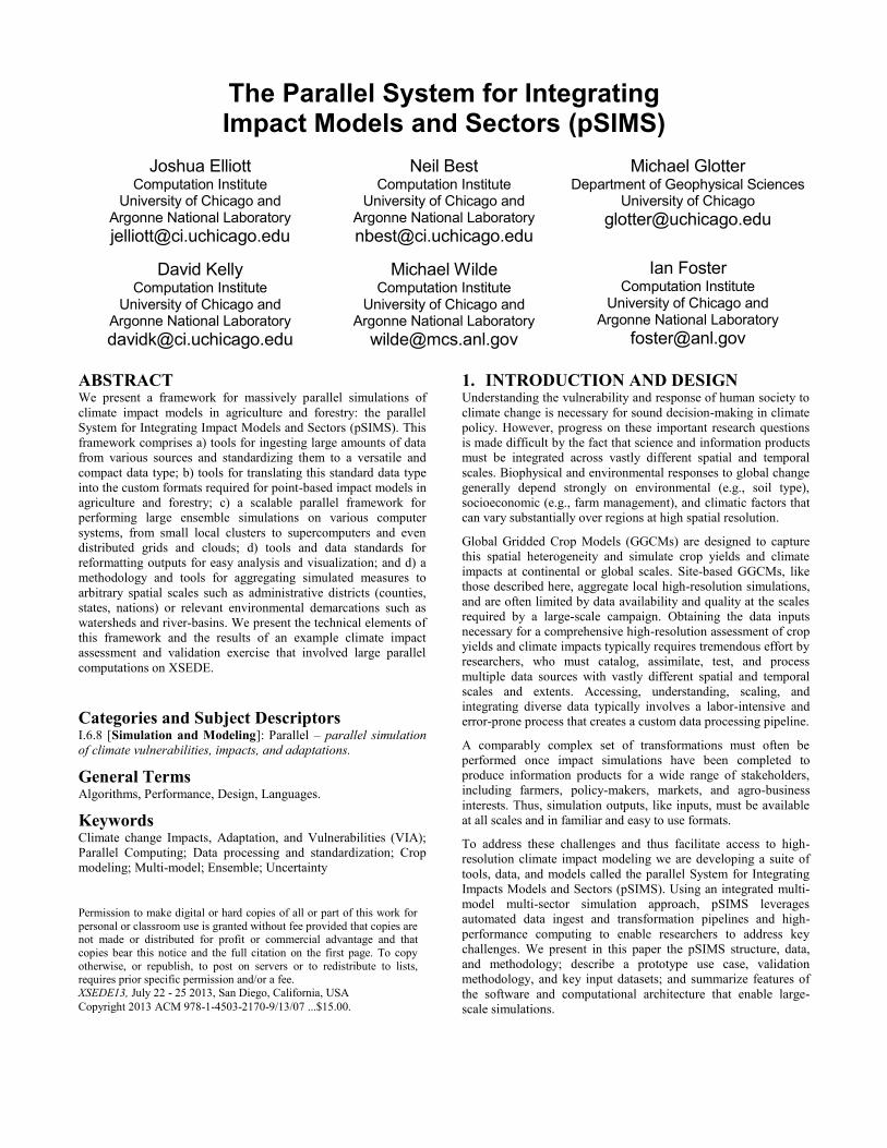
Figure 1 shows the principal elements of pSIMS including both
automated steps (the focus of this paper) and those that require an
interactive component (such as specification and aggregation).
The framework is separated into four major components: data
ingest and standardization, user initiated campaign specification,
parallel implementation of specified simulations, and aggregation
to arbitrary decision-relevant scales.
pSIMS is designed to support integration of any point-based
climate impact model that requires standard daily weather data as
inputs. We developed the framework prototype with versions 4.0
and 4.5 of the Decision Support System for Agrotechnology
Transfer (DSSAT [15]). DSSAT 4.5 supports models of 28
distinct crops using two underlying biophysical models (CERES
and CropGRO). Additionally, we have prototyped and tested a
parallel version of the CenW [16] forest growth simulation model
and are actively integrating additional crop yield and climate
impact models starting with the widely used Agricultural
Production Systems Simulator (APSIM) [23]. As of this writing,
continental- to global-scale simulation experiments ranging in
resolution from 3–30 arcminutes have been conducted on four
crop and 1 tree (pinus radiata) species using a variety of
weather/climate inputs and scenarios.
2. THE pSIMS DATA INPUT PIPELINE The minimum weather data requirements for crop and climate
impact models such as DSSAT, APSIM, and CenW are typically:
Daily maximum temperature (degrees C at 2m above the ground surface)
Daily minimum temperature (degrees C at 2m)
Daily average downward shortwave radiation flux (W/m2
measured at the ground surface)
Total daily Precipitation (mm/day at the ground surface)
In addition, it is also sometimes desirable to include daily average
wind speeds and surface humidity if available.
Hundreds of observational datasets, model-based reanalyses, and
multi-decadal climate model simulation outputs at regional and
global scales exist that can be used to drive climate impact
simulations. For some use-cases, one or another data product may
be demonstrably superior, but most often a clear understanding of
the range of outcomes and uncertainty requires simulations with
an ensemble of inputs. For this reason, input data requirements for
high-resolution climate impact experiments can be large and data
processing and management can be challenging.
One major challenge in dealing with long daily time-series of
high-resolution weather data is that input products are typically
stored one or more variables at a time in large spatial raster files
segmented into annual, monthly, or sometimes even daily or sub-
daily time-slices. Point-based impact models on the other hand,
typically require custom ASCII data types that encode long time-
series of daily data for all required variables for a single point into
one file. The process of accessing hundreds or thousands of
spatial raster files O(105–106) times to extract the time-series for
each point is time-consuming and expensive [20]. To ameliorate
this challenge, we have established a NetCDF4-based data-type
for the pSIMS framework—identified by a .psims.nc4
extension—and tools for translating existing archives into this
format (Figure 2).
Each .psims.nc4 file represents a single grid cell or simulation site
within the study area. Its contents are one or more 1 x 1 x T
arrays, one per variable, where T is the number of time steps. The
time coordinates of each array are explicit in the definition of their
dimensions, a strategy that facilitates near-real-time updates from
upstream sources. The spatial coordinates of each array are also
explicit in the definition of their dimensions, which facilitates
downstream spatial merging. Variables are grouped and named so
as to avoid namespace collisions with variables from other
sources in downstream merging, e.g.. “narr/tmax” refers to daily
maximum temperature variable extracted from the North
American Regional Reanalysis (NARR) dataset and “cfsrr/tmax”
to the daily minimum temperature from the NOAA Climate
Forecast System Reanalysis and Reforecast (CFSRR) dataset.
Because a given .psims.nc4 file contains information about a
single point location, the longitude and latitude vectors used as
Figure 1: Schematic of the pSIMS workflow. 1) Data ingest takes data from numerous publicly available archives in arbitrary file formats and data types. 2) The standardization step reconstitutes each of these datasets into the highly portable point-based .psims.nc4 format. 3) The specification step defines a
simulation campaign for pSIMS by choosing a .psims.nc4 dataset or subset and one or more climate impact models (and the requisite custom input and
output data translators) from the code library. 4) The translation step individual .psims.nc4 files (each representing one grid-cell in the spatial simulation) are converted into the custom file formats required by the models. 5) In the simulation step, individual simulation calls within the campaign are managed
by Swift on the available high-performance resource. 6) In the output reformatting step, model outputs (dozens or even hundreds of time-series variable
from each run) are extracted from model-specific custom output formats and translated into a standard .psims.out format. 7) Finally, in the aggregation
step, output variables are masked as necessary and aggregated to arbitrary decision-relevant spatial or temporal scales.
array dimensions are both of length one. Therefore the typical
weather variable is represented as a 1x1xT array where T is the
number of time steps in the source data. In contrast, arrays
containing forecast variables have two time dimensions, the time
the forecast is made and the time of the prediction. This use of
two time dimensions makes it possible to follow the evolution of a
series of forecasts made over a period of time for a particular
future date, as for example when forecasts of crop yields at a
particular location are refined over time as more information
becomes available..
pSIMS input files are named according to (row, col) tuple in the
global grid and organized in a file structure similarly (e.g.,
/narr/361/1168/361_1168.psims.nc4) so that the terminal
directories hold data for a single site. This improves the
performance of parallel reads and writes on shared filesystems
like GPFS and minimizes clutter while browsing the tree. Because
files represent points, the resolution is only set by the organization
of the enclosing directory tree and is recorded in an archive
metadata file, as well as in the metadata of each .psims.nc4 file.
Climate data from observations and simulations is widely
available in open and easily accessible archives, such as those
accessible by Earth System Grid (ESG) [30], NCAR’s NOMADS
servers [26], and NASA’s Modeling and Assimilation Data
Information Services Center (MDISC). These datasets have
substantial metadata—often based on Climate and Forecasting
(CF) conventions [8]—and are frequently identified by a unique
Digital Object Identifier (DOI) [21], making provenance and
tracking relatively straightforward. Such data is often archived at
uniform grid resolutions, but scales can vary from a few
kilometers to one or more degrees and frequencies from an hour
to a month. Furthermore, different map projections mean that
transformations are sometimes necessary before data can be used.
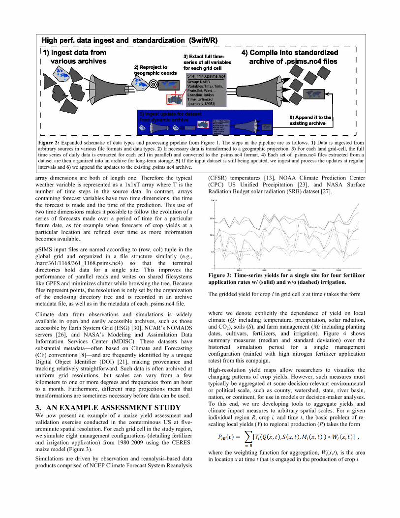
3. AN EXAMPLE ASSESSMENT STUDY We now present an example of a maize yield assessment and
validation exercise conducted in the conterminous US at five-
arcminute spatial resolution. For each grid cell in the study region,
we simulate eight management configurations (detailing fertilizer
and irrigation application) from 1980-2009 using the CERES-
maize model (Figure 3).
Simulations are driven by observation and reanalysis-based data
products comprised of NCEP Climate Forecast System Reanalysis
(CFSR) temperatures [13], NOAA Climate Prediction Center
(CPC) US Unified Precipitation [23], and NASA Surface
Radiation Budget solar radiation (SRB) dataset [27].
Figure 3: Time-series yields for a single site for four fertilizer
application rates w/ (solid) and w/o (dashed) irrigation.
The gridded yield for crop i in grid cell x at time t takes the form
where we denote explicitly the dependence of yield on local
climate (Q; including temperature, precipitation, solar radiation,
and CO2), soils (S), and farm management (M; including planting
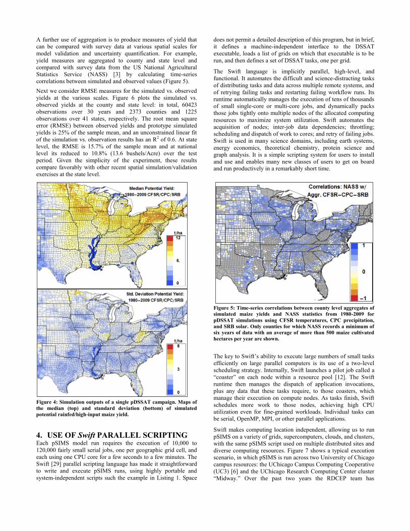
dates, cultivars, fertilizers, and irrigation). Figure 4 shows
summary measures (median and standard deviation) over the
historical simulation period for a single management
configuration (rainfed with high nitrogen fertilizer application
rates) from this campaign.
High-resolution yield maps allow researchers to visualize the
changing patterns of crop yields. However, such measures must
typically be aggregated at some decision-relevant environmental
or political scale, such as county, watershed, state, river basin,
nation, or continent, for use in models or decision-maker analyses.
To this end, we are developing tools to aggregate yields and
climate impact measures to arbitrary spatial scales. For a given
individual region R, crop i, and time t, the basic problem of re-
scaling local yields (Y) to regional production (P) takes the form
where the weighting function for aggregation, Wi(x,t), is the area
in location x at time t that is engaged in the production of crop i.
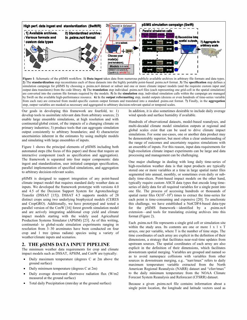
Figure 2: Expanded schematic of data types and processing pipeline from Figure 1. The steps in the pipeline are as follows. 1) Data is ingested from
arbitrary sources in various file formats and data types. 2) If necessary data is transformed to a geographic projection. 3) For each land grid-cell, the full
time series of daily data is extracted for each cell (in parallel) and converted to the .psims.nc4 format. 4) Each set of .psims.nc4 files extracted from a dataset are then organized into an archive for long-term storage. 5) If the input dataset is still being updated, we ingest and process the updates at regular
intervals and 6) we append the updates to the existing .psims.nc4 archive.
A further use of aggregation is to produce measures of yield that
can be compared with survey data at various spatial scales for
model validation and uncertainty quantification. For example,
yield measures are aggregated to county and state level and
compared with survey data from the US National Agricultural
Statistics Service (NASS) [3] by calculating time-series
correlations between simulated and observed values (Figure 5).
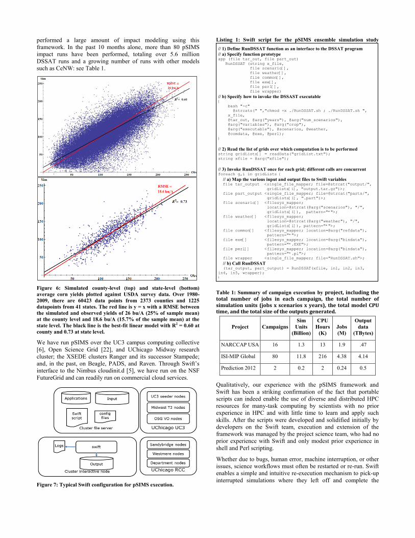
Next we consider RMSE measures for the simulated vs. observed
yields at the various scales. Figure 6 plots the simulated vs.
observed yields at the county and state level: in total, 60423
observations over 30 years and 2373 counties and 1225
observations over 41 states, respectively. The root mean square
error (RMSE) between observed yields and prototype simulated
yields is 25% of the sample mean, and an unconstrained linear fit
of the simulation vs. observation results has an R2 of 0.6. At state
level, the RMSE is 15.7% of the sample mean and at national
level its reduced to 10.8% (13.6 bushels/Acre) over the test
period. Given the simplicity of the experiment, these results
compare favorably with other recent spatial simulation/validation
exercises at the state level.
Figure 4: Simulation outputs of a single pDSSAT campaign. Maps of
the median (top) and standard deviation (bottom) of simulated
potential rainfed/high-input maize yield.
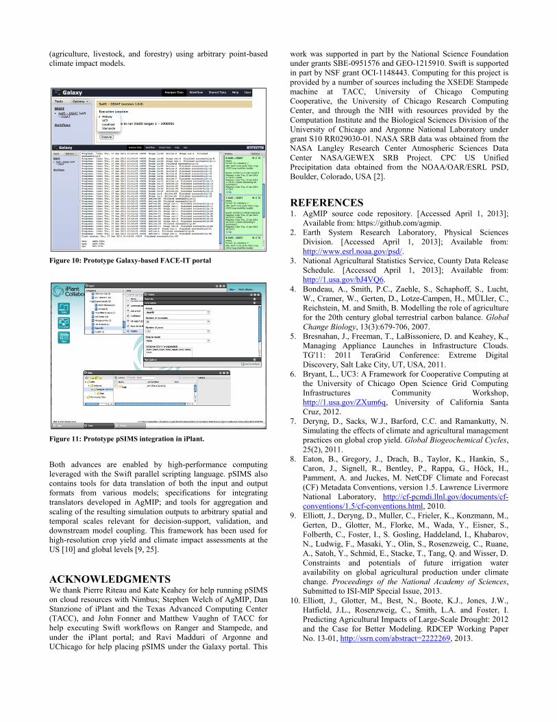
4. USE OF Swift PARALLEL SCRIPTING Each pSIMS model run requires the execution of 10,000 to
120,000 fairly small serial jobs, one per geographic grid cell, and
each using one CPU core for a few seconds to a few minutes. The
Swift [29] parallel scripting language has made it straightforward
to write and execute pSIMS runs, using highly portable and
system-independent scripts such the example in Listing 1. Space
does not permit a detailed description of this program, but in brief,
it defines a machine-independent interface to the DSSAT
executable, loads a list of grids on which that executable is to be
run, and then defines a set of DSSAT tasks, one per grid.
The Swift language is implicitly parallel, high-level, and
functional. It automates the difficult and science-distracting tasks
of distributing tasks and data across multiple remote systems, and
of retrying failing tasks and restarting failing workflow runs. Its
runtime automatically manages the execution of tens of thousands
of small single-core or multi-core jobs, and dynamically packs
those jobs tightly onto multiple nodes of the allocated computing
resources to maximize system utilization. Swift automates the
acquisition of nodes; inter-job data dependencies; throttling;
scheduling and dispatch of work to cores; and retry of failing jobs.
Swift is used in many science domains, including earth systems,
energy economics, theoretical chemistry, protein science and
graph analysis. It is a simple scripting system for users to install
and use and enables many new classes of users to get on board and run productively in a remarkably short time.
Figure 5: Time-series correlations between county level aggregates of
simulated maize yields and NASS statistics from 1980-2009 for
pDSSAT simulations using CFSR temperatures, CPC precipitation,
and SRB solar. Only counties for which NASS records a minimum of
six years of data with an average of more than 500 maize cultivated
hectares per year are shown.
The key to Swift’s ability to execute large numbers of small tasks
efficiently on large parallel computers is its use of a two-level
scheduling strategy. Internally, Swift launches a pilot job called a
“coaster” on each node within a resource pool [12]. The Swift
runtime then manages the dispatch of application invocations,
plus any data that these tasks require, to those coasters, which
manage their execution on compute nodes. As tasks finish, Swift
schedules more work to those nodes, achieving high CPU
utilization even for fine-grained workloads. Individual tasks can
be serial, OpenMP, MPI, or other parallel applications.
Swift makes computing location independent, allowing us to run
pSIMS on a variety of grids, supercomputers, clouds, and clusters,
with the same pSIMS script used on multiple distributed sites and
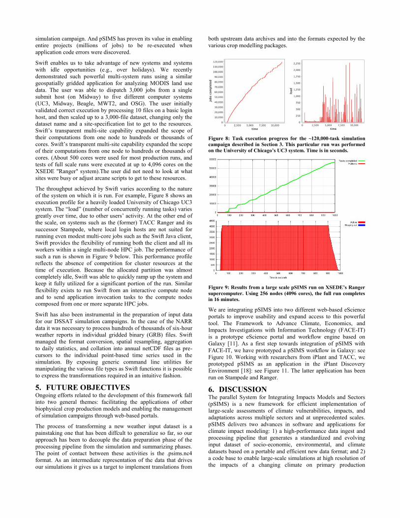
diverse computing resources. Figure 7 shows a typical execution
scenario, in which pSIMS is run across two University of Chicago
campus resources: the UChicago Campus Computing Cooperative
(UC3) [6] and the UChicago Research Computing Center cluster
“Midway.” Over the past two years the RDCEP team has
performed a large amount of impact modeling using this
framework. In the past 10 months alone, more than 80 pSIMS
impact runs have been performed, totaling over 5.6 million
DSSAT runs and a growing number of runs with other models
such as CeNW: see Table 1.
Figure 6: Simulated county-level (top) and state-level (bottom)
average corn yields plotted against USDA survey data. Over 1980-
2009, there are 60423 data points from 2373 counties and 1225
datapoints from 41 states. The red line is y = x with a RMSE between
the simulated and observed yields of 26 bu/A (25% of sample mean)
at the county level and 18.6 bu/A (15.7% of the sample mean) at the
state level. The black line is the best-fit linear model with R2 = 0.60 at
county and 0.73 at state level.
We have run pSIMS over the UC3 campus computing collective
[6], Open Science Grid [22], and UChicago Midway research
cluster; the XSEDE clusters Ranger and its successor Stampede;
and, in the past, on Beagle, PADS, and Raven. Through Swift’s
interface to the Nimbus cloudinit.d [5], we have run on the NSF
FutureGrid and can readily run on commercial cloud services.
Figure 7: Typical Swift configuration for pSIMS execution.
Listing 1: Swift script for the pSIMS ensemble simulation study
Table 1: Summary of campaign execution by project, including the total number of jobs in each campaign, the total number of simulation units (jobs x scenarios x years), the total model CPU time, and the total size of the outputs generated.
Project Campaigns
Sim
Units
(Billion)
CPU
Hours
(K)
Jobs
(M)
Output
data
(TBytes)
NARCCAP USA 16 1.3 13 1.9 .47
ISI-MIP Global 80 11.8 216 4.38 4.14
Prediction 2012 2 0.2 2 0.24 0.5
Qualitatively, our experience with the pSIMS framework and
Swift has been a striking confirmation of the fact that portable
scripts can indeed enable the use of diverse and distributed HPC
resources for many-task computing by scientists with no prior
experience in HPC and with little time to learn and apply such
skills. After the scripts were developed and solidified initially by
developers on the Swift team, execution and extension of the
framework was managed by the project science team, who had no
prior experience with Swift and only modest prior experience in
shell and Perl scripting.
Whether due to bugs, human error, machine interruption, or other
issues, science workflows must often be restarted or re-run. Swift
enables a simple and intuitive re-execution mechanism to pick-up
interrupted simulations where they left off and complete the
// 1) Define RunDSSAT function as an interface to the DSSAT program
// a) Specify function prototype app (file tar_out, file part_out)
RunDSSAT (string x_file,
file scenario[],
file weather[],
file common[],
file exe[],
file perl[],
file wrapper)
// b) Specify how to invoke the DSSAST executable {