Journal of Electromyography and Kinesiology 21 (2011) 423–432

Contents lists available at ScienceDirect

Journal of Electromyography and Kinesiology

journal homepage: www.elsevier .com/locate / je lek in

The peak-to-peak ratio of single-fibre potentials is little influenced by changesin the electrode positions close to the muscle fibre q

Javier Rodríguez a,*, Javier Navallas a, Luis Gila b, Ignacio Rodríguez a, Armando Malanda a

a Public University of Navarra, Department of Electrical and Electronic Engineering, 31006 Pamplona, Spainb Virgen del Camino Hospital, Department of Clinical Neurophysiology, 31008 Pamplona, Spain

a r t i c l e i n f o

Article history:Received 21 December 2009Received in revised form 6 April 2010Accepted 6 April 2010

Keywords:Single fibre action potentialPeak-to-peak ratioIAP spatial profileRadial distanceDipole character

1050-6411/$ - see front matter � 2010 Elsevier Ltd. Adoi:10.1016/j.jelekin.2010.04.001

q The present work was carried out at the Public UniSpain. Recordings were made at the Virgen del CamClinical Neurophysiology, Pamplona, Spain.

* Corresponding author. Address: Universidad Púbpus de Arrosadia s/n., 31006 Pamplona, Spain. Tel.: +169720.

E-mail address: javier.rodriguez.falces@gmail.com

a b s t r a c t

In a series of previous works we studied the ratio between the amplitudes of the second and first phases(the peak-to-peak ratio) of single fibre action potential (SFAPs) using the Dimitrov–Dimitrova SFAPconvolutional model as a reference. From experimental potentials extracted from both healthy anddiseased muscles, we determined typical peak-to-peak ratio (PPR) values and ranges for both normaland pathological conditions. In addition, we investigated the changes observed in the PPR of consecutivepotentials recorded at different fibre-to-electrode distances. However, our results were not conclusivedue to insufficient data. The objective of the present work was to obtain a more concrete descriptionof the relation between PPR and radial distance. To this end, we recorded 135 sets of consecutive SFAPsfrom the m. tibialis anterior of four normal subjects. The needle was intentionally moved whilst recordingeach SFAP set. We found that PPR was largely independent of small changes in electrode position whenthe electrode was close to the fibre and sufficiently far from the neuromuscular and/or fibre–tendon junc-tions. In the discussion, we provide evidence that this result is in agreement with the generation of extra-cellular potentials considering the spatial extension of the intracellular action potential (IAP) along thefibre.

� 2010 Elsevier Ltd. All rights reserved.

1. Introduction

Characteristics of single fibre action potentials (SFAPs) gener-ated by the propagation of an action potential along a muscle fibreare known to depend essentially on the shape of the intracellularaction potential (IAP) (Plonsey, 1974, 1977; Nandedkar andStålberg, 1983; Dimitrov and Dimitrova, 1998) as well as on the fi-bre-to-electrode distance (hereafter referred to as radial distance).However, direct control of the radial distance has not yet provedfeasible in EMG studies (Van Veen et al., 1993). This explains thatthe search of parameters in the SFAP waveform independent fromchanges in the position of the needle had attracted the attention ofinvestigators. Using simulations Nandedkar and Stålberg (1983)and Dimitrov and Dimitrova (1989) found that the peak-to-peaktime interval (sometimes referred to as SFAP rise-time) hardlychanges with electrode positions within 150–200 lm from thefibre axis. A recent experimental study (Rodriguez et al., 2010)

ll rights reserved.

versity of Navarra, Pamplona,ino Hospital, Department of

lica de Navarra D.I.E.E., Cam-34 948 169094; fax: +34 948

(J. Rodríguez).

has confirmed that the rise-time of SFAPs is practically not influ-enced by changes in radial distance when the electrode is movedin the immediate vicinity of the fibre. This raises the question ofwhether there might be other SFAP shape parameters independentof positional changes of the needle.

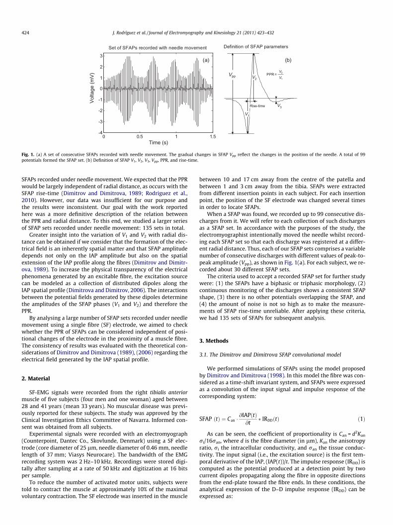
EMG studies have directed some effort towards understandingthe relation between the amplitudes of the first positive phase(V1) and second negative phase (V2) of extracellular potentials(see Fig. 1(b)) (Dimitrov and Dimitrova, 1974; Miller-Larsson,1985). The concept of the peak-to-peak ratio (PPR) of a SFAP, de-fined as the absolute value of the quotient of V2 over V1, was intro-duced by the current authors in 2006 (Rodriguez et al., 2006) but atthat time was only studied in a small collection of fibrillationpotentials. Our preliminary studies were extended in a recent work(Rodriguez et al., 2009) in which we recorded a large number ofSFAPs from the right tibialis anterior muscle of four normal sub-jects. With this new data, we determined typical PPR values andranges: all PPR histograms had a well-defined single peak around1.0, and PPR ranged from about 0.3 to 2.5. We noticed that a num-ber of spurious factors, such as, proximity of the electrode to theneuromuscular or fibre–tendon junctions, baseline fluctuation, orthe finite sampling rate, could change artifactually the PPR value.

In Rodriguez et al. (2009) we also studied changes in the PPRs ofconsecutive potentials recorded at different fibre-to-electrode dis-tances. To do this, we analysed the PPR variations in 23 sets of

Vpp

Rise-time

(b)

0 0.5 1 1.5-4

-3

-2

-1

0

1

2

3

Definition of SFAP parametersSet of SFAPs recorded with needle movement

(a)

V1

V2

V2

V1

PPR =

V3

Time (s)

Volta

ge (m

V)

Fig. 1. (a) A set of consecutive SFAPs recorded with needle movement. The gradual changes in SFAP Vpp reflect the changes in the position of the needle. A total of 99potentials formed the SFAP set. (b) Definition of SFAP V1, V2, V3, Vpp, PPR, and rise-time.

424 J. Rodríguez et al. / Journal of Electromyography and Kinesiology 21 (2011) 423–432

SFAPs recorded under needle movement. We expected that the PPRwould be largely independent of radial distance, as occurs with theSFAP rise-time (Dimitrov and Dimitrova, 1989; Rodriguez et al.,2010). However, our data was insufficient for our purpose andthe results were inconsistent. Our goal with the work reportedhere was a more definitive description of the relation betweenthe PPR and radial distance. To this end, we studied a larger seriesof SFAP sets recorded under needle movement: 135 sets in total.

Greater insight into the variation of V1 and V2 with radial dis-tance can be obtained if we consider that the formation of the elec-trical field is an inherently spatial matter and that SFAP amplitudedepends not only on the IAP amplitude but also on the spatialextension of the IAP profile along the fibres (Dimitrov and Dimitr-ova, 1989). To increase the physical transparency of the electricalphenomena generated by an excitable fibre, the excitation sourcecan be modeled as a collection of distributed dipoles along theIAP spatial profile (Dimitrova and Dimitrov, 2006). The interactionsbetween the potential fields generated by these dipoles determinethe amplitudes of the SFAP phases (V1 and V2) and therefore thePPR.

By analysing a large number of SFAP sets recorded under needlemovement using a single fibre (SF) electrode, we aimed to checkwhether the PPR of SFAPs can be considered independent of posi-tional changes of the electrode in the proximity of a muscle fibre.The consistency of results was evaluated with the theoretical con-siderations of Dimitrov and Dimitrova (1989), (2006) regarding theelectrical field generated by the IAP spatial profile.

2. Material

SF-EMG signals were recorded from the right tibialis anteriormuscle of five subjects (four men and one woman) aged between28 and 41 years (mean 33 years). No muscular disease was previ-ously reported for these subjects. The study was approved by theClinical Investigation Ethics Committee of Navarra. Informed con-sent was obtained from all subjects.

Experimental signals were recorded with an electromyograph(Counterpoint, Dantec Co., Skovlunde, Denmark) using a SF elec-trode (core diameter of 25 lm, needle diameter of 0.46 mm, needlelength of 37 mm; Viasys Neurocare). The bandwidth of the EMGrecording system was 2 Hz–10 kHz. Recordings were stored digi-tally after sampling at a rate of 50 kHz and digitization at 16 bitsper sample.

To reduce the number of activated motor units, subjects weretold to contract the muscle at approximately 10% of the maximalvoluntary contraction. The SF electrode was inserted in the muscle

between 10 and 17 cm away from the centre of the patella andbetween 1 and 3 cm away from the tibia. SFAPs were extractedfrom different insertion points in each subject. For each insertionpoint, the position of the SF electrode was changed several timesin order to locate SFAPs.

When a SFAP was found, we recorded up to 99 consecutive dis-charges from it. We will refer to each collection of such dischargesas a SFAP set. In accordance with the purposes of the study, theelectromyographist intentionally moved the needle whilst record-ing each SFAP set so that each discharge was registered at a differ-ent radial distance. Thus, each of our SFAP sets comprises a variablenumber of consecutive discharges with different values of peak-to-peak amplitude (Vpp), as shown in Fig. 1(a). For each subject, we re-corded about 30 different SFAP sets.

The criteria used to accept a recorded SFAP set for further studywere: (1) the SFAPs have a biphasic or triphasic morphology, (2)continuous monitoring of the discharges shows a consistent SFAPshape, (3) there is no other potentials overlapping the SFAP, and(4) the amount of noise is not so high as to make the measure-ments of SFAP rise-time unreliable. After applying these criteria,we had 135 sets of SFAPs for subsequent analysis.

3. Methods

3.1. The Dimitrov and Dimitrova SFAP convolutional model

We performed simulations of SFAPs using the model proposedby Dimitrov and Dimitrova (1998). In this model the fibre was con-sidered as a time-shift invariant system, and SFAPs were expressedas a convolution of the input signal and impulse response of thecorresponding system:

SFAP ðtÞ ¼ Can �@IAPðtÞ@t

� IRDDðtÞ ð1Þ

As can be seen, the coefficient of proportionality is Can = d2Kan

ri/16ran, where d is the fibre diameter (in lm), Kan the anisotropyratio, ri the intracellular conductivity, and ran the tissue conduc-tivity. The input signal (i.e., the excitation source) is the first tem-poral derivative of the IAP, (IAP(t))/t. The impulse response (IRDD) iscomputed as the potential produced at a detection point by twocurrent dipoles propagating along the fibre in opposite directionsfrom the end-plate toward the fibre ends. In these conditions, theanalytical expression of the D–D impulse response (IRDD) can beexpressed as:

J. Rodríguez et al. / Journal of Electromyography and Kinesiology 21 (2011) 423–432 425

IRDDðr; mtÞ ¼ m � ðz0 � mtÞ½ðz0 � mtÞ2 þ kan � r2�

32

ð2Þ

where r is the radial distance (in mm), z0 the longitudinal distanceof the electrode (in mm), and m the propagation velocity (in m/s).We shall refer to r, z0, Kan, d, and m as impulse response parametersand except when we vary one of them in the course of our study,their values will be set to r = 0.085 mm, Kan = 5 (as suggested byRosenfalck, 1969; Griep et al., 1978; Andreassen and Rosenfalck,1981), and d = 55 lm (as suggested by Nandedkar and Stålberg,1983; Nandedkar and Sanders, 1988). Note that in (2) only thesource propagating to the right is considered. Calculation of thepropagation velocity of a fibre with diameter d was performedaccording to the equation (Nandedkar and Stålberg, 1983; Nanded-kar and Sanders, 1988):

mðm=sÞ ¼ 4þ 0:05 � ðd� 55Þ ð3Þ

We considered a 90 mm long fibre with a right semilength of40 mm. We used a reference velocity of 4 m/s and a time step(sampling interval) of 1 ls (1000 kHz). This means that the spacestep used for the simulations is 4 lm, which is suitable for the ra-dial distances of interest (20–300 lm).

In order to investigate the effects of the neuromuscular and fi-bre–tendon junction on the PPR, we used the IAP approximationproposed by Arabadzhiev et al. (2008) that computes the wholeIAP time course using a single analytical description:

IAPðtÞ ¼ A1½ðA3t3 þ A2t2 � A4A5t � A5Þe�A4 �t þ A5�e�A6 �t ð4Þ

The coefficient values used for normal muscle fibres wereA1 = 1029, A2 = 9, A3 = 1, A4 = 7.5, A5 = 0.015, A6 = 0.045. They pro-vided an IAP with Tdep = 250 ls, a value close to that measuredby Ludin (1969) in humans or Wallinga et al. (1985) in rats.

3.2. Simulation and experimental studies

3.2.1. Simulation studiesBy changing the longitudinal position of the electrode (z0), we

investigated how the proximity of the neuromuscular and fibre–tendon junctions affects the SFAP PPR. To appreciate the PPRchanges better, close to neuromuscular junction, z0 was decreasedfrom 0.8 to 0.3 mm in steps of 0.1 mm, and close to the fibre–ten-don junction, z0 was increased from 39.4 to 39.9 mm in steps of0.1 mm. The rest of the impulse response parameters were set totheir default values.

Electrode close to the end-plate(r = 0.85 mm )

Volta

ge (m

V)

0 0.2 0.4 0.6 0.8 1

-1

-0.5

0

0.5

1

1.5

2 (a)1 0.3 3.212 0.4 2.153 0.5 1.554 0.6 1.335 0.7 1.226 0.8 1.16

SFAP z0(mm) PPR

12

34

56

Time (ms)

Fig. 2. Effects of an electrode moving longitudinally towards the neuromuscul

3.2.2. Experimental studiesWhen the needle is moved whilst recording a SFAP set, the ra-

dial distance varies, but, we assume that the excitation sourceand propagation velocity are not affected. However, direct controlof the radial distance has not yet proved feasible in EMG studies(Van Veen et al., 1993). Considering the radial decline of the SFAPamplitude reported by other authors (Ekstedt and Stålberg, 1973),we assumed that the changes in the amplitude of consecutiveSFAPs produced by needle movement reflected variations in the fi-bre–electrode distance.

For each of the consecutive discharges in a SFAP set, we mea-sured the PPR and Vpp. Then, we depicted the PPR and Vpp valuesof these discharges in a PPR–Vpp space. The resulting PPR–Vpp dia-grams enable us to study the variations of PPR associated withchanges in Vpp within each set of SFAPs.

Because PPR–Vpp diagrams are formed by a set of points, therepresentation and comparison of various SFAP sets in the samePPR–Vpp diagram is not convenient. To overcome this problemwe fitted a linear regression line to each set of points within aPPR–Vpp diagram. Thus, each SFAP set is described by a gradient(mi). The sign of mi reflects whether PPR increases or decreaseswith Vpp (and therefore with r), whereas the absolute value of mi

indicates the strength of the PPR–Vpp (and the PPR–r) dependence.Our use of linear regression lines to represent PPR–Vpp diagramshas three main advantages: (1) it provides a simple and accurateapproximation of SFAP sets; (2) it enables visual comparison ofseveral sets in a single PPR–Vpp diagram; and (3) it enables, bygrouping all mi values in the same histogram, statistical analysisof the PPR–Vpp relation.

4. Results

4.1. Simulation results

Fig. 2(a) shows the changes in the shape of the SFAPs producedby an electrode approaching longitudinally to the neuromuscularjunction. As can be seen, the SFAPs second phases are almost un-changed (V2 varies very little), whereas their first phases are signif-icantly reduced. Therefore, the PPR of a SFAP increases as therecording point gets closer to the end-plate. The PPR values corre-sponding to each position of the electrode are indicated in thefigure.

Fig. 2(b) shows the alterations in the SFAP waveforms producedby an electrode coming closer longitudinally to the fibre–tendonjunction. In this case, a significant amplitude reduction is appreci-

10.5 11 11.5

-1

-0.5

0

0.5

1

1.5

2 (b)1 39.4 1.162 39.5 1.093 39.6 0.954 39.7 0.755 39.8 0.526 39.9 0.43

12

34 5

6

SFAP z0(mm) PPR

Electrode close to the tendon(r = 0.85 mm )

Time (ms)

ar junction (a) and to the fibre–tendon junction (b) on the PPR of a SFAP.

426 J. Rodríguez et al. / Journal of Electromyography and Kinesiology 21 (2011) 423–432

ated in the second phases of the SFAPs, whilst their first phases re-main almost constant. Thus, the SFAP PPR is expected to decreaseas the recording point gets closer to the tendon.

4.2. Experimental results

For each of our 135 sets of SFAPs, we calculated the PPR–Vpp

diagram. The diagrams obtained can be roughly divided into threedistinct types. In the second row of Fig. 3 there is a representativediagram of each type. In these diagrams, the linear regression linesare drawn with solid lines. The top row of Fig. 3 shows the needlemovements from which these three PPR–Vpp diagrams wereobtained.

0.4 0.6 0.8 1 1.2

-1

0

1

0 1 2 3 4 5

0.5

1

1.5

0 0.2 0.4

-5

0

5

10

0.5 1

0.5

1

1.5

2m = 0.01 m = 0.92

Volta

ge (m

V)

Vpp (mV)

PPR

Vpp

Needle movement, type I Needle movx 10 -1

(a)

(d)

Time (s) Tim

Fig. 3. Three different samples of needle movements (top row) with their correspondingradient of each regression line is given towards the top of each PPR–Vpp diagram. Theconsiderably: in (d) PPR does not change with Vpp, in (e) PPR increases with Vpp, where

0

5

10

15

20

25

30

35

0 0.1 0.2 0.3 0.4-0.1-0.2-0.3-0.40.0

0.5

1.0

1.5

2.0

2.5

0.0 1.0 2.0

Vpp (m

PP

R

Slopes (mi) of regression lines

Nº

of r

epet

ition

s

(a)

Regression lines with

mi > 0.4

Slope histogram

mi < - 0.4

Fig. 4. (a) Histogram of the slopes of the regression lines calculated for 135 sets of SFAPs�0.052 and a standard deviation of 0.21. Representation of all the linear regression curdepicted in (b) and (c) are approximately horizontal, which is consistent with the slope hby the lower-PPR bound of 0.5 and an upper-PPR bound of 1.5.

By visual inspection of the needle movement of type I (Fig. 3(a)),we realize that both the V1 and V2 of the consecutive discharges de-crease in a similar proportion as Vpp is reduced. As a result, in thePPR–Vpp diagram of Fig. 3(d), the slope of the regression line, m1, isvery close to 0, showing that PPR hardly changes with Vpp (andtherefore with r).

Fig. 3(b) is an example of needle movement of type II. In thiscase, changes in the position of the needle affect V2 more thanV1: note that V1 changes less. As a consequence, the gradient m2

of the PPR–Vpp regression line in Fig. 3(e) is positive and steep. Gi-ven the inverse relation between Vpp and r, this positive slope indi-cates that PPR decreases with radial distance.

The third type of needle movement observed is represented inFig. 3(c). In this case, changes in the position of the needle affect

0.6 0.8 1 1.2 1.4 1.60.2

0.4

0.6

0.8

1

1.2

0.6 0.8 0 0.1 0.2 0.3 0.4

-10

-5

0

5

1.5 2

m = -1.1

(mV) Vpp (mV)

ement, type II Needle movement, type IIIx 10 -1

(b)

(c)

(e)

(f)

e (s) Time (s)

g PPR–Vpp diagrams (second row). The solid line is the linear regression line; therelation between the PPR and Vpp of the three different needle movements differs

as in (f) PPR decreases with Vpp.

3.0 4.0 5.00.0

0.5

1.0

1.5

2.0

2.5

0.0 1.0 2.0 3.0 4.0 5.0

V) Vpp (mV)

PP

R

)c()b(

negative slopes Regression lines with positive slopes

. The profile of the histogram approximates to a normal distribution, with a mean ofves with slopes greater than 0 (b) and less than 0 (c). Note that most of the linesistogram shown in (a). Note also that most of these lines fall within an area limited

J. Rodríguez et al. / Journal of Electromyography and Kinesiology 21 (2011) 423–432 427

V1 while V2 remains relatively untouched. Consequently, theregression line that describes the PPR–Vpp diagram (Fig. 3(f)) hasa markedly negative slope. Based on the relation between Vpp

and r, this indicates that PPR increases with r.By grouping the gradients of the regression lines corresponding

to our 135 SFAP sets recorded with needle movement, we obtainedthe histogram of Fig. 4(a). As can be seen, this histogram has,approximately, a normal distribution, with a mean of �0.052 anda standard deviation of 0.21. Of the regression lines, 73% had gra-dients between �0.2 and 0.2, indicating that the PPRs in most ofthe SFAP sets hardly changed with Vpp.

In order to visualize and compare the different variations of PPRwith Vpp observed in all of our SFAP sets we plotted, in the samePPR–Vpp space, the linear regression lines corresponding to theseSFAP sets. Regression lines with positive and negative slopes, rep-resented in Fig. 4(b) and (c), respectively, are representedseparately.

In Fig. 4(b) and (c), regression lines can be seen to share somecharacteristics. First, in both diagrams most lines are roughly hor-izontal, as one would expect on the basis of the large number ofgradients with an absolute value close to 0 in the histogram ofFig. 4(a). Second, in both diagrams most lines lie within an arealimited by a lower-PPR limit of 0.5 and an upper-PPR limit of 1.5.This result is in good agreement with previous reports for poten-tials recorded using a single fibre electrode (Rodriguez et al.,2006, 2009). Finally, note that most lines with a steep gradient

0 1 2 3 4 50

20

40

60

80

100

–

+ +-– +- +- +- +- +- +- +- +- +- +- +- +- +- +- +–A1

A3 A4 A5 B12B11B10B9 B8 B7 B6 B5 B4 B3

B1

Volta

ge(m

V)

Spatial length (mm)

Spatial length (mm)

+

- +

+ –+

depolarization-repolarization distance

Dipoles distributed along the IAP spatial pr

r1Rad

ial d

ista

nce

(a.u

.)

+

++ - - +- +- +- +- +- +- +- +- +- +

+ -+ -+ -

+ -+-+-+-

+-+-+-+-

+-+-+-+-

+-+-+-+-

+-+-+-+-

+-+-+-+-

+-+-+-+-

+-+-+-+-

+-+-+-+-

+-+-+-+-

+-+-+-+-

+-

Double-layered disks representing the IAP spatial p

Muscle fibre(a)

(b)

(c)p1

+ -+ -+ -

+ -+ -+ -+ -

+ -+ -+ -+ -

+ -+ -+ -+ -

+ -

(DRD)

– – – – – – – – – –+++++++r3

r2

Polarity of the extracellular potential

B2A2

++

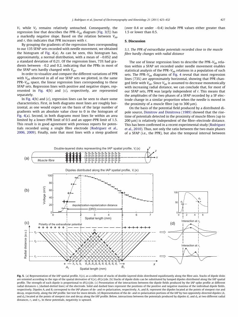
Fig. 5. (a) Representation of the IAP spatial profile, Vi(x), as a collection of stacks of doubare oriented according to the sign of the spatial derivative of Vi(x), dVi(x)/dx. (b) Stacks ofprofile. The strength of each dipole is proportional to dVi(x)/dx. (c) Presentation of the inradial distances ri (dashed-dotted lines) of the electrode. Solid and dashed lines represenrespectively. Dipoles Ai and Bi correspond to the IAP phases of de- and re-polarization, redecay, respectively, along the IAP profile. See text for more details. (d) Representation of tand d2) located at the points of steepest rise and decay along the IAP profile. Below, interdistances, r1 and r3. In these potentials, negativity is upward.

(over 0.4 or under �0.4) include PPR values either greater than1.5 or lower than 0.5.

5. Discussion

5.1. The PPR of extracellular potentials recorded close to the musclefibre hardly changes with radial distance

The use of linear regression lines to describe the PPR–Vpp rela-tion within a SFAP set recorded under needle movement enablesstatistical analysis of the PPR–Vpp relations in a population of suchsets. The PPR–Vpp diagrams of Fig. 4 reveal that most regressionlines (73%) are approximately horizontal, showing that PPR chan-ged little with Vpp. Since Vpp is assumed to decrease monotonicallywith increasing radial distance, we can conclude that, for most ofour SFAP sets, PPR was largely independent of r. This means thatthe amplitudes of the two phases of a SFAP recorded by a SF elec-trode change in a similar proportion when the needle is moved inthe proximity of a muscle fibre (up to 300 lm).

On the basis of the potential field produced by a distributed di-pole source, Dimitrov and Dimitrova (1989) showed that the rise-time of potentials detected in the proximity of muscle fibres (up to200 lm) is relatively independent of the fibre–electrode distance.This has been confirmed in a recent experimental study (Rodriguezet al., 2010). Thus, not only the ratio between the two main phasesof a SFAP (i.e., the PPR), but also the temporal interval between

0 2 4 60

50

100

6 7

ofile, Vi (x)

x

x

zyrofile, Vi (x)

– – – –+++++++Interaction at r3

Interaction at r1

(d)

d1

d2– +

–+

- +- +- +- +- +- +- + - +

le-layered disks distributed equidistantly along the fibre axis. Stacks of dipole disksdipole disks can be substituted by lumped dipoles distributed along the IAP spatialteractions between the dipole fields produced by the IAP spike profile at differentt the positions of the positive and negative maxima of the individual dipole fields,

spectively. A1 and B1 represent the dipoles located at the points of steepest rise andhe de- and re-polarization portions of the IAP by two oppositely-directed dipoles (d1

actions between the potentials produced by dipoles d1 and d2 at two different radial

428 J. Rodríguez et al. / Journal of Electromyography and Kinesiology 21 (2011) 423–432

them (i.e., the rise-time) change very little when the recordingelectrode is moved in the immediate vicinity of the fibre. In sum-mary, up to a certain distance from the fibre, two recordings ofthe same SFAP made at different radial distances will basically dif-fer only in a scale factor.

5.2. Studying the PPR considering the IAP spatial profile

The formation of an electrical field around a fibre is an inher-ently spatial matter (Dimitrova, 1973; Dimitrova and Dimitrov,2006). This means that the amplitudes of the SFAP phases (V1, V2,and V3), the relationships between them (such as the PPR), andtheir dependence with radial distance depend not only on theIAP amplitude, but also on the spatial extension of the IAP alongthe fibre.

On the basis of Appendix 1, the IAP spatial profile, Vi(x), can berepresented by stacks of double-layered disks distributed equidis-tantly along the fibre axis (Fig. 5(a)). Since one such disk producesa dipole field, we can substitute each disk by a lumped dipole (Wil-son et al., 1933) and, therefore, we can imagine the IAP spatial pro-file as a collection of distributed dipoles, as shown in Fig. 5(b). Thestrength of each of the dipoles (or dipole moment) is determinedby the spatial derivative of the potential profile along the fibre[dVi(x)/dx]. In Fig. 5(b), the differences in the strengths of the dis-tributed dipoles are represented by the different sizes of the posi-tive and negative charges. Orientation of the dipoles is determinedby the sign of dVi(x)/dx.

To better conceive how the electrical field develops, in Fig. 5(c)each dipole is substituted by a solid and a dashed line representingthe positions of the positive and negative maxima, respectively, ofthe field produced by this dipole at different distances from the di-pole axis (see Appendix 2 for details). In the figure, the dipoles lo-cated at the points of steepest rise (A1) and decay (B1) along the IAPprofile can be easily identified by their corresponding lines, whichare thicker than the others. The spatial distance between A1 and B1,hereafter referred to as the depolarization–repolarization distance(DRD), is an important parameter as it influences the interactionsbetween the different dipoles. For the sake of clarity, dipoles tothe left of A1 and to the right of B1 have been omitted. Thestrengths of dipoles Ai and Bi decrease as they approach the posi-tion at which the IAP spatial profile is maximum. It should be men-tioned that Dimitrova and Dimitrov (2002), (2003), (2006) used the2-dipoles version of the IAP spatial profile presentation when thefeatures of potential field produced at large distances from an ac-tive fibre were considered.

The polarity of the extracellular potential that results from theinteractions between all distributed dipoles is represented by thepositive and negative signs at the top of Fig. 5(c). All the dipolesfrom the IAP rising and falling phases give rise to the positivephases of the SFAP. The negative region of the summated field liesapproximately between dipoles A1 and B1 (dashed lines) and givesrise to the negative phase of the SFAP. Therefore, the amplitude ofthis phase, V2, is determined by interactions between the negativemaxima lines of dipoles Ai and Bi.

In Fig. 5(c) radial distances are represented in the y-axis, i.e.,perpendicular to the fibre’s longitudinal axis. For sake of simplicity,we assume that z = 0, and therefore y = r. Interactions between thefields of the oppositely-directed dipoles depend on the radial dis-tance considered. For small values of r, such as r1, interaction be-tween the negative maxima of dipoles Ai and Bi is small (in thepicture, only the negative maxima lines of A4 and A5 coincide withthose of B12 and B11, respectively). As r increases, more and moredipoles with stronger moments start interacting. When r = r2, forexample, the negative maxima lines of A2, A3, A4 and A5 coincidewith those of B5, B4, B3 and B2, respectively, which makes V2 in-crease. At the same radial distance, r2, interaction between positive

and negative fields begins (i.e., the negative maxima line of B12 en-ters the positive region of the field generated by dipole A1), whichmakes V1 decrease. Therefore, an increase in r should be accompa-nied by an increase in PPR.

For a given value of DRD, an optimal radial distance exists, atwhich the negative maxima of A1 and B1 coincide (Fig. 5(c), pointp1). This radial distance can be calculated approximately asr3 = DRD/

p2 mm (Dimitrova, 1973). However, the fact that the

negative maxima lines coincide at r3, does not guarantee that theSFAP PPR reach its maximum value at this distance. This is becausethe PPR is a ratio between two parameters, V1 and V2, each onewith a different dependence on DRD (Dimitrov and Dimitrova,1974). Nevertheless, we could say that, at DRD/

p2 mm, the PPR

should be close to its maximum value.The increasing of PPR with radial distance can be also under-

stood by observing Fig. 5(d). In this figure, the IAP phases of de-and re-polarization are represented by two oppositely-directed di-poles (d1 and d2) located at the points of steepest rise and decayalong the IAP spatial profile. Below this IAP profile, we show thepotentials produced by dipoles d1 and d2 at two different radial dis-tances, r1 and r3. As can be seen, at r1 the potential profiles corre-sponding to d1 and d2 overlap only slightly. However, at r3 thepotential profiles of d1 and d2 overlap so that the positions of theircorresponding maximums coincide. As a result, in the summatedpotential, a large increase in V2 relative to V1 occurs, which in turnmakes PPR reach a very high value.

5.2.1. Is the presentation of the IAP in the spatial domain consistentwith our needle movements?

A question arises whether the theory of the dipoles distributedalong the IAP spatial profile, shown above, is in agreement withthe PPR–r relation demonstrated by our needle movements. Tocheck this numerically, let us consider the measurements fromIAPs recorded experimentally by Wallinga et al. (1985). Wal-linga’s group found that the depolarization–repolarization dura-tion was, on average, 0.5 ms for the m. extensor digitorumlongus and 0.70 ms for the soleus muscle of a rat, respectively.By assuming that the propagation velocity of the excitation wavesis 4 m/s (Nandedkar and Stålberg, 1983; Nandedkar and Sanders,1988), then the depolarization–repolarization distance (DRD)would vary approximately within the range 2.0–2.8 mm in nor-mal IAPs. If we consider a DRD of 2 mm, then the radial distanceat which there will be optimal summation of the negative max-ima lines of the dipoles representing the IAP will occur at r � 2/p

2 = 1.41 mm. Therefore, within the radial distances typical inSFEMG recordings (less than 0.3 mm), the interactions betweenthe oppositely-directed fields generated by these dipoles shouldbe practically absent. As a result, the decreasing of V1 and V2 withr would be equivalent and the PPR would accordingly remain al-most constant.

5.3. The dipole character of the excitation source in the proximity ofthe muscle fibre

If the fibre–electrode distance (0.05–0.2 mm) is much shorterthan the depolarization–repolarization distance (2.0–2.8 mm),then the distances between the point of observation and the indi-vidual dipoles distributed along the IAP spatial profile will differsignificantly. As a result, the magnitude of the recorded SFAP isdetermined mainly by the dipoles closest to the electrode, andthe interaction between oppositely-directed dipole fields pro-duced by IAP depolarization and repolarization phases is weak.In such a case, the dipole field produced by the IAP depolarizationphase is considerably stronger, because the dipoles are distrib-uted at a considerably shorter fibre region. This means that theindividual dipoles have a higher strength and their fields have a

J. Rodríguez et al. / Journal of Electromyography and Kinesiology 21 (2011) 423–432 429

better spatial summation than those corresponding to the longerspatial length of the IAP repolarization phase. Thus, in the prox-imity of the fibre, the characteristics of SFAPs essentially dependon the spatial length of the rising phase of the IAP, as stated byvarious authors (Dimitrov and Dimitrova, 1989; Dumitru, 1994;Arabadzhiev et al., 2008). Since, in these conditions, the electricalfield is generated by dipoles oriented in the same direction, thesource is said to have dipole character (Dimitrova and Dimitrov,2002).

5.4. Needle movements where PPR changes significantly with Vpp

The PPR–Vpp diagrams of Fig. 4(b) and (c) show that in 27% ofthe SFAP sets recorded under needle movements the PPR has astrong correlation (either positive or negative) with Vpp. Presum-ably, in these SFAP sets, changes in radial distance affect the PPRsignificantly. Does this mean that in 27% of our SFAP sets the exci-tation source does not have dipole character? What other technicalfactors or physiological phenomena could account for this variabil-ity in the PPR?

We have no means to check whether the excitation source hasdipole character in these SFAPs. However, there are several aspectsof the recording process that may introduce artifactual variation inthe PPR: proximity of the electrode to the neuromuscular or fibre–tendon junctions, angulation or rotation of the electrode, baselinefluctuation, changes in tissue conductivity, errors due to the finitesampling rate of the EMG recording system, and random noise.Without having further evidence, it seems that the last three ofthe above factors are largely random and therefore cannot easilyexplain a high correlation between PPR and Vpp. Baseline drift overconsecutive discharges, however, could introduce some trend inconsecutive discharges as to change artifactually the PPR and cre-ate an apparent correlation between PPR and Vpp.

Proximity of the recording electrode to neuromuscular or fibre–tendon junctions may also account for the observed PPR variations.Indeed, simulation results of Fig. 2(a) and (b) demonstrated thatsuch proximity could affect the PPR even without changing radialdistance. Since the tibialis anterior muscle has a pennate architec-ture with an extensive central aponeurosis and widely distributedend-plates (Aquilonius et al., 1984; Wolf and Kim, 1997), it is likelythat some of the SFAPs in our study will have been recorded closeto neuromuscular and/or fibre–tendon junctions and potentiallyaffected by such proximity. The fact that in some needle move-ments one of the SFAP phases remains practically unchanged, asin Fig. 3(b) and (c), support this hypothesis. Further evidence tosupport this argument is that, in the PPR–Vpp diagrams ofFig. 4(b) and (c), most regression lines with steep slopes also havevery low or very high PPR values, which suggests that the corre-sponding SFAP sets were recorded close to the neuromuscularand/or fibre–tendon junctions.

Angulation and rotation of the cannula could also affect thePPR artifactually, especially in muscles such as the tibialis ante-rior: with a pennate architecture and wide end-plate distribution.The effect of rotation changes of the cannula on the SFAP wave-form was studied by Theeuwen et al. (1993). However, no exper-imental studies have been carried out to validate the theoreticalpredictions.

On the basis of the interactions between the fields generated bythe dipoles distributed along the IAP profile, the PPR should alwaysincrease with increasing radial distance (see Section 5.2 for de-tails). However, only in 56% of the PPR–Vpp diagrams (those whoseregression lines have negative slopes) did PPR increase with r. Howcan there be such a large percentage of SFAP sets (44%) inconsis-tent with theoretical prediction? The explanation lies in the factthat, at radial distances typical for SF EMG recordings (less than0.3 mm), the interactions between the opposite-in-sign potential

fields produced by the dipoles representing the excitation sourceare very weak. Consequently, the PPR will change only slightlywith radial distance. In such conditions, factors extraneous to thedipoles action, such as the proximity of the recording point toeither the end-plate or tendon, can affect one of the SFAP phasesmore than radial distance, thereby obscuring the true dependenceof PPR on r.

5.5. Future studies

Although we assimilated a large number of recordings withneedle movement for the present study, future studies areneeded to fully establish that changes in PPR with radial dis-tance are almost negligible when the electrode moves within aradius of 300 lm from the fibre. Such further studies should in-volve muscles with a narrowly-distributed end-plate region andwith few pennate fibres, such as the extensor digitorum commu-nis or the biceps brachii. In such muscles, at short radial dis-tances, we would expect to find no correlation between PPRand SFAP amplitude.

Finally, recordings with needle movement from muscles withneuromuscular disorders would also be very interesting. In dis-eased muscles there are noticeable alterations in the IAP waveformand duration. Ludin (1973) found that the duration of the IAPdepolarization phase in dystrophic human muscle fibres was sig-nificantly longer. Abnormal calcium accumulation in myopathicmuscle fibres (Bertorini et al., 1991; Imbert et al., 1995, 1996; Gil-lis, 1999; Han et al., 2006) can increase the IAP spike duration andthe negative after potential (Ishiko and Sato, 1957). Thus, these dis-eases would alter the spatial distribution of the dipole sourcesalong the IAP profile, modifying the sensitivity of PPR to changesin radial distance.

6. Conclusions

1. We found that PPR was practically not influenced by changes inSFAP amplitude (and therefore of radial distance) in 73 percentof 135 SFAPs sets recorded under needle movement with a sin-gle fibre electrode. This suggest that if the recording of consec-utive potentials is not affected by factors extraneous to thedipole action, then the amplitudes of the two phases of a SFAPwill change in a similar proportion when the needle is moved inthe proximity of a muscle fibre (up to 300 lm).

2. Modeling the excitation source as a collection of distributeddipoles along the IAP spatial profile is a useful approach forunderstanding how the SFAP waveform changes with radialdistance.

3. Since interactions between the oppositely-directed fields gener-ated by the dipoles representing the IAP spatial profile increasewith increasing radial distance, the SFAP peak-to-peak ratio(PPR) should always increase when an electrode is drawn awayfrom a fibre. However, inside the 300 lm radius within whichSFAPs are usually detected, interactions between dipole fieldsare weak, and so the PPR is predicted be largely independentof changes in the positions of the electrode. At such radial dis-tances, the IAP spatial profile can be assumed to have the char-acteristics of a dipole.

Acknowledgement

This work was supported by the Spanish Ministry of Education& Science under the project SAF2007-65383.

430 J. Rodríguez et al. / Journal of Electromyography and Kinesiology 21 (2011) 423–432

Appendix A

A.1. Modeling of the excitation wave using double-layered disks

Any skeletal muscle is activated by electrical impulses comingfrom alpha-motoneurons through their axons (myelinated nervefibres). Activation of an excitable cell results in its depolarizationand generation of the transmembrane voltage across its mem-brane. As the extracellular potential is much smaller than theintracellular potential the term intracellular action potential (IAP)is predominantly used instead of transmembrane voltage.

In muscle fibre, the membrane depolarization excites neighbourregions at both sides from the end-plate located somewhere in themiddle portion of the fibre (Fig. 6(a)). As a result, two IAPs propa-gate in an all-or-nothing way (i.e., without decrement) with prop-agation velocity v along the muscle fibre towards its ends wherethey extinguish. Since the intracellular potential is mainly nega-tive, In Fig. 6(a) the polarization of the fibre membrane is repre-sented by a number of layers of negative signs. When themembrane is at rest, the number of negative-signed layers is con-stant. However, at any moment after the fibre activation, two po-tential profiles exist across the fibre membrane that are calledwaves of excitation or depolarized zones (Fig. 6(a)). The numberof negative-signed layers within the depolarized zones of the fibrechanges progressively with axial distance (x-axis in the figure) sothat an IAP profile has gradual depolarization and repolarizationtransitions, as shown in Fig. 6(b). The length of the IAP profile alongthe fibre, b, is defined by the product of the IAP duration, Tin, andpropagation velocity v (Fig. 6(b)).

The profile of the IAP can be represented (Fig. 6(d)) through anumber of steps of equal length dx that are opened at their endsand uniformly depolarized according to the mean IAP value atthe corresponding membrane portions. Two layers with different

- - - - - - - - - - - - - - - - - - - - - - - - - - - - - - - - - - - - - - - - - - - - - - - - -- - - - - - - - - - - - - - - - - - - - - - - - - - - - - - - - - - - - - - - - - - - - - - - - -- - - - - - - - - - - - - - - - - - - - - - - - - - - - - - - - - - - - - - - - - - - - - - - - -- - - - - - - - - - - - - - - - - - - - - - - - - - - - - - - - - - - - - - - - - - - - - - - - -- - - - - - - - - - - - - - - - - - - - - - - - - - - - - - - - - - - - - - - - - - - - - - - - -

- - - - - - - - - - - - - - - - - - - - - - - - - - - - - - - - - - - - - - - - - - - - - - - - -- - - - - - - - - - - - - - - - - - - - - - - - - - - - - - - - - - - - - - - - - - - - - - - - -- - - - - - - - - - - - - - - - - - - - - - - - - - - - - - - - - - - - - - - - - - - - - - - - -- - - - - - - - - - - - - - - - - - - - - - - - - - - - - - - - - - - - - - - - - - - - - - - - -- - - - - - - - - - - - - - - - - - - - - - - - - - - - - - - - - - - - - - - - - - - - - - - - -

(depolarized zones of the fibre)

IAPs propagating along the fibre

restingfibre

resting fibre

restingfibre

v

v

end-plate

IAPs in spatial domain

depolarizationtransition

repolarizationtransition

b = Tin·v

(b)

(a)

(cMotorneuron

axon

x

z

y

+ + + + + + + + + + + + + + + + + + + + + + + + + + + + + + + + + +

+ + + + + + + + + + + + + + + + + + + + + + + + + + + + + + + + + +

v

Fig. 6. (a) Schematic presentation of a muscle fibre innervated by the axon of a motonelayers of negative signs. Two depolarized zones propagate along the fibre from the endepolarized zones changes gradually with axial distance and is constant within the regi(IAP) with its de- and re-polarization phases. (c) IAP potential profile along the fibre mem(black and white disks). (d) Approximation of IAP profile through a number of steps of eqthe mean IAP value at the corresponding membrane portions. Modified from Dimitrovencyclopedia of biomedical engineering. Hoboken, NJ: John Wiley and Sons; 2006. Repr

polarity (represented by the disks of different, white and black, col-or) arise at the boundaries between two steps (Fig. 6(d)). On thebasis of the studies of Wilson et al. (1933), each of these layers(or disks) generates a potential equivalent to that of a dipole. Thesummated effect of the oppositely-polarized layers can be repre-sented through a disk whose dipole moment is defined by the dif-ference in IAPs produced at neighbour segments, i and i + 1, of thefibre. As a result, an actual excitation wave can be represented(Wilson et al., 1933; Plonsey, 1974) by two stacks of double-lay-ered disks distributed equidistantly along the fibre axis (Fig. 6(c),black and white disks). Orientation of the dipoles is identical ineach stack and opposite in different stacks. Thus, calculation ofthe extracellular potential can be reduced to the sum of the poten-tials produced by the disks distributed along the fibre axis (Dimitr-ova, 1973). A similar presentation of the fibre as the one shown inFig. 6 can be found in Dimitrova and Dimitrov (2006).

Appendix B

B.1. Potential field produced by a lumped dipole

Considering the source across the fibre membrane as two stacksof distributed dipoles (Fig. 6(d)), it is useful to remember potentialfield produced by a lumped (point) dipole. Fig. 7(a) shows a dipole(positive and negative charges in the middle of the figure) and itscorresponding equipotential lines at the plane of the paper, sche-matically represented by solid and dotted circles (for positiveand negative dipole fields, respectively). The dipole produces a 3-dimensional potential field that is zero everywhere in the planethat is perpendicular to the dipole axis and passes through its mid-point (Fig. 7(a), projection of the plane, i.e., zero line, is along thedashed y-axis). The plane divides the space into two regions, one

- - - - - - - - - - - - - - - - - - - - - - - - - - - - - - - - - - - - - - - - - - - - - - - - - - - - - - - - -

- - - - - - - - - - - - - - - - - - - - - - - - - - - - - - - - - - - - - - - - - - - - - - - - - - - - - - - - -- - - - - - - - - - - - - - - - - - - - - - - - - - - - - - - - - - - - - - - - - - - - - - - - - - - - - - - - -- - - - - - - - - - - - - - - - - - - - - - - - - - - - - - - - - - - - - - - - - - - - - - - - - - - - - - - - -- - - - - - - - - - - - - - - - - - - - - - - - - - - - - - - - - - - - - - - - - - - - - - - - - - - - - - - - -- - - - - - - - - - - - - - - - - - - - - - - - - - - - - - - - - - - - - - - - - - - - - - - - - - - - - - - - -- - - - - - - - - - - - - - - - - - - - - - - - - - - - - - - - - - - - - - - - - - - - - - - - - - - - - - - - -- - - - - - - - - - - - - - - - - - - - - - - - - - - - - - - - - - - - - - - - - - - - - - - - - - - - - - - - -- - - - - - - - - - - - - - - - - - - - - - - - - - - - - - - - - - - - - - - - - - - - - - - - - - - - - - - - -- - - - - - - - - - - - - - - - - - - - - - - - - - - - - - - - - - - - - - - - - - - - - - - - - - - - - - - - -- - - - - - - - - - - - - - - - - - - - - - - - - - - - - - - - - - - - - - - - - - - - - - - - - - - - - - - - -- - - - - - - - - - - - - - - - - - - - - - - - - - - - - - - - - - - - - - - - - - - - - - - - - - - - - - - - -

+ + + + + + + + + + + + + + + + + + + + + + + + + + + + + + + + + + + + + + + +

Detail of a depolarization zone of a muscle fibre

(d)

)

++++

----

++++

----

++++

----

++++

----

++++

----

++++

----

++++

----

++++

----

++++

----

++++

----

++++

----

IAP profile

x

dx

IAP profile

i i+1

++++

----

+-+-

Resting fibre Resting fibre

uron at the end-plate. Polarization of the fibre membrane is represented by severald-plate region to the fibre ends. The number of negative-signed layers within theons where the fibre is at rest. (b) Spatial profile of the intracellular action potentialbrane can be considered as two stacks of dipole disks oriented in opposite directionsual length dx that are opened at their ends and uniformly depolarized according to

a NA, Dimitrov GV. Electromyography (EMG) modeling. In: Metin A, editor. Wileyinted with permission of John Wiley and Sons, Inc.

Lumped (point) dipole

+ 0

y3y2y1

+

a+

A+

x = 0.7yi

Y

Y

d

X

X

(a)

(b)

0

yi

A

a

x = 0.7yi

a+ a

+

(c)

Fig. 7. (a) Schematic drawing of the potential field produced by a lumped (point)dipole (black point in the centre of the figure). Signs (+) and (�) near the pointdenote location of the positive and negative point charges that constitute thedipole. The circles depict equipotential lines of the positive (solid lines) andnegative (dotted lines) fields produced by the dipole. a+ and a� denote points ofextreme potential along the line y = y3. See text for more details. (b) Lines denotedby A+ and A� represent position of the extreme points at different distances fromthe dipole axis. (c) Potentials produced by a lumped dipole along the lines located atdistances y = y1, y2, y3 from the dipole axis. Negativity is upward. Dimitrova NA,Dimitrov GV. Electromyography (EMG) modeling. In: Metin A, editor. Wileyencyclopedia of biomedical engineering. Hoboken, NJ: John Wiley and Sons; 2006.Reprinted with permission of John Wiley and Sons, Inc.

J. Rodríguez et al. / Journal of Electromyography and Kinesiology 21 (2011) 423–432 431

with positive and one with negative potentials denoted by (+) and(–), respectively.

At a certain radial distance, y, from the dipole axis (Fig. 7(a),lines for y = y1, y2, y3), the maximal potential is produced at thepoints a + and a–. They coincide with the tangency points (depictedby black spots) of the corresponding line and the equipotentiallines. The larger the radial distance, the further from the zero lineis the corresponding maximum (Fig. 7(a), black spots and Fig. 7(b)lines A+ and A�). For any distance y, the extremes points a+ and a�are at distances x = ± y/

p2 � 0.7�y from the zero line (Fig. 7(b)). The

potential produced by the dipole along a line located at a certaindistance from the dipole axis, u(x)|y, is biphasic, positive–negative(Fig. 7(c), u(x) for y = y1, y2, y3). The presentation of the dipole fieldas explained in this appendix was introduced by Dimitrova andDimitrov (2006).

References

Andreassen S, Rosenfalck A. Relationship of intracellular and extracellular actionpotentials of skeletal muscle fibers. CRC Crit Rev Bioeng 1981;7:267–306.

Aquilonius SM, Askmark H, Gillberg PG, Nandedkar S, Olsson Y, Stålberg E.Topographical localization of motor end-plates in cryosections of wholehuman muscles. Muscle Nerve 1984;7(4):287–93.

Arabadzhiev T, Dimitrov GV, Chakarov V, Dimitrov A, Dimitrova NA. Effects ofchanges in intracellular action potential on potentials recorded by single-fiber,macro, and belly-tendon electrodes. Muscle Nerve 2008;37(6):700–12.

Bertorini T, Palmieri G, Griffin J, Igarashi M, Hinton A, Karas J. Effect of dantrolene inDuchenne muscular dystrophy. Muscle Nerve 1991;14:503–7.

Dimitrov GV, Dimitrova NA. Influence of the asymmetry in the distribution of thedepolarization level on the extracellular potential field generated by anexcitable fibre. Electromyogr Clin Neurophysiol 1974;14:255–75.

Dimitrov GV, Dimitrova NA. Extracellular potentials produced by a transitionbetween an inactive and active regions of an excitable fibre. Electromyogr ClinNeurophysiol 1989;29:265–71.

Dimitrov GV, Dimitrova NA. Precise and fast calculation of the motor unit potentialsdetected by a point and rectangular plate electrode. Med Eng Phys1998;20:374–81.

Dimitrova NA. Influence of the length of the depolarized zone on the extracellularpotential field of a single unmyelinated nerve fibre. Electromyogr ClinNeurophysiol 1973;13:547–58.

Dimitrova NA, Dimitrov GV. Amplitude-related characteristics of motor unit and M-wave potentials during fatigue. A simulation study using literature data onintracellular potential changes found in vitro. J Electromyogr Kinesiol2002;12:339–49.

Dimitrova NA, Dimitrov GV. Interpretation of EMG changes with fatigue: facts,pitfalls, and fallacies. J Electromyogr Kinesiol 2003;13(1):13–36.

Dimitrova NA, Dimitrov GV. Electromyography (EMG) modeling. In: Metin A, editor.Wiley encyclopedia of biomedical engineering. Hoboken, NJ: John Wiley andSons; 2006.

Dumitru D. The biphasic morphology of voluntary and spontaneous SFAPs. MuscleNerve 1994;17:1301–7.

Ekstedt J, Stålberg E. How the size of the needle electrode leading-off surfaceinfluences the shape of the single muscle fibre action potential inelectromyography. Comp Prog Biomed 1973;3:204–12.

Gillis J. Understanding dystrophinopathies: an inventory of the structural andfunctional consequences of the absence of dystrophin in muscles of the mdxmouse. J Muscle Res Cell Motil 1999;20:605–25.

Griep PAM, Boon KL, Stegeman DF. A study of the motor unit action potential bymeans of computer simulation. Biol Cybern 1978;30:221–30.

Han R, Grounds M, Bakker A. Measurement of sub-membrane [Ca2+] in adultmyofibres and cytosolic [Ca2+] in myotubes from normal and mdx mice usingthe Ca2+ indicator FFP-18. Cell Calcium 2006;40:299–307.

Imbert N, Cognard C, Duport G, Guillou C, Raymond G. Abnormal calciumhomeostasis in Duchenne muscular dystrophy myotubes contracting in vitro.Cell Calcium 1995;18:177–86.

Imbert N, Vanderbrouck C, Constantin B, Duport G, Guillou C, Cognard C.Hypoosmotic shocks induce elevation of resting calcium level in Duchennemuscular dystrophy myotubes contracting in vitro. Neuromuscul Disord1996;6:351–60.

Ishiko N, Sato M. The effect of calcium ions on electrical properties of striatedmuscle fibres. Jpn J Physiol 1957;7:51–63.

Ludin H. Action potentials of normal and dystrophic human muscle fibers. In:Desmedt JE, editor. New development in electromyography and clinicalneurophysiology. Basel: Karger; 1973. p. 400–6.

Ludin HP. Microelectrode study of normal human skeletal muscle. Eur Neurol1969;2:340–7.

Miller-Larsson A. An analysis of extracellular single muscle fiber. Biol Cybern1985;51:271–84.

Nandedkar S, Sanders DB. Simulation of concentric needle EMG motor unit actionpotentials. Muscle Nerve 1988;11:151–9.

Nandedkar S, Stålberg E. Simulation of single muscle fibre action potentials. MedBiol Eng Comput 1983;21:158–65.

Plonsey R. The active fiber in a volume conductor. IEEE Trans Biomed Eng1974;21:371–81.

Plonsey R. Action potential sources and their volume conductor fields. Proc IEEE1977;65:601–11.

Rodriguez J, Malanda A, Gila A, Rodriguez I, Navallas J. Modelling fibrillationpotentials – a new analytical description for the muscle intracellular actionpotential. IEEE Trans Biomed Eng 2006;53:581–92.

Rodriguez J, Malanda A, Gila A, Rodríguez I, Navallas J. Analysis of the peak-to-peakratio of extracellular potentials in the proximity of excitable fibres. JElectromyogr Kinesiol. [Accepted 28.07.2009] [Epub ahead of print].

Rodriguez J, Navallas J, Gila L, Rodriguez I, Malanada A. Relationship between therise-time of single fibre action potentials and radial distance in human musclefibres. Clin Neurophisiol. 2010;121:214–20.

Rosenfalck P. Intra- and extracellular fields of active nerve and muscle fibers. Aphysico-mathematical analysis of different models. Acta Physiol Scand1969;321:1–168.

Theeuwen MM, Gootzen TH, Stegeman DF. Muscle electric activity. I: a model studyon the effect of needle electrodes on single fiber action potentials. Ann BiomedEng 1993;21(4):377–89.

432 J. Rodríguez et al. / Journal of Electromyography and Kinesiology 21 (2011) 423–432

Van Veen BK, Wolters H, Wallinga W. The bioelectrical source in computing singlemuscle fiber action potentials. Biophys J 1993;64:1492–8.

Wallinga W, Gielen FLH, Wirtz P, de Jong P, Broenink J. The different intracellularaction potentials of fast and slow muscle fibres. Electromyogr Clin Neurophysiol1985;60:539–47.

Wilson FN, MacLeod AG, Barker PS. The distribution of the action currents producedby heart muscle and other excitable tissues immersed in extensive conductingmedia. J Gen Physiol 1933;16:423–56.

Wolf SL, Kim JH. Morphologycal analysis of the human tibialis anterior and medialgastrocnemius muscles. Acta Anat (Basel) 1997;158(4):287–95.

Javier Rodríguez Falces was born in Pamplona in 1979.He graduated in 2003, and obtained the Ph.D. in 2007 inTelecommunication Engineering from the Public Uni-versity of Navarra, Pamplona, Spain. He worked as aConsultant Engineer (2004–2005) and as a SystemEngineer (2005–2006) in the private sector. He has alsoworked for the Higher Scientific Investigation Council ofSpain during one year (2006). In 2007 he becameAssistant Professor in the Electrical and ElectronicsEngineering Department of the Public University ofNavarra. During this period he has been teaching severalsubjects related to digital signal processing, imageprocessing and biomedical engineering. His researchfocuses on signal processing applied to biomedical sig-

nals, modeling of biological systems, electromyography and sensory-motor inter-action studies.

Javier Navallas Irujo was born in Pamplona in 1976. Hegraduated in 2002, and he obtained the Ph.D. in 2008 inTelecommunication Engineering from the Public Uni-versity of Navarra, Pamplona, Spain. He has also workedas a software engineer. He is presently Assistant Pro-fessor of the Electrical and Electronics EngineeringDepartment of this University. His research interests aremodeling of biological systems and neurosciences.

Luis Gila Useros received his MD degree from theComplutense University, Madrid, Spain in 1983. In 1988he completed his specialization in Neurology at the‘‘Ramón y Cajal” Hospital, Madrid. Between 1989 and1998 he worked as a neurologist at the ‘‘San Millán”Hospital, Logroño, Spain. From 1998 to 2001 he carriedout his specialization training in Clinical Neurophysi-ology at the ‘‘Virgen del Camino” Hospital, Pamplona,Spain, where at the present time he is a staff member atthe Department of Clinical Neurophysiology. Hisresearch interests include quantitative electromyogra-phy and the automatic analysis of electromyographicsignals.

Ignacio Rodriguez Carreño was born in Madrid in1976. In 2000 he obtained his degree in Telecommuni-cation Engineering from the Public University of Nava-rre, Pamplona, Spain. In 2001 he worked as an engineerin the development of software and hardware forcommunications systems. In 2002 he joined the PublicUniversity of Navarre as Assistant Professor of theDepartment of Electrical and Electronics Engineeringand he started his doctoral courses. Since 2003 he hasbeen granted a research fellowship by the NavarraGovernment to complete his Ph.D. His area of researchis the development of software and algorithmic meth-ods for the processing of EMG signals.

Armando Malanda Trigueros was born in Madrid,Spain, in 1967. In 1992 he graduated in Telecommuni-cation Engineering at the Madrid Polytechnic Univer-sity. In 1999 he received his Ph.D. degree from theCarlos III University, Madrid. In 1992 he joined theSchool of Telecommunication and Industrial Engineer-ing of the Public University of Navarra. In 2003 hebecame Associate Professor in the Electrical and Elec-tronics Engineering Department of this University.During all this period he has been teaching severalsubjects related to digital signal processing, imageprocessing and biomedical engineering. His areas ofinterest comprise the analysis, modeling and simulationof bioelectrical signals, particularly EEG and EMG.