The Pennsylvania State University The Graduate School SEMI ...

The Pennsylvania State University

The Graduate School

College of Engineering

SEMI-ACTIVE CONTROL OF HELICOPTER VIBRATION

USING CONTROLLABLE STIFFNESS AND DAMPING DEVICES

A Thesis in

Aerospace Engineering

by

Phuriwat Anusonti-Inthra

Submitted in Partial Fulfillmentof the Requirements

for the Degree of

Doctor of Philosophy

August 2002

We approve the thesis of Phuriwat Anusonti-Inthra.

Date of Signature

Farhan GandhiAssociate Professor of Aerospace EngineeringThesis AdvisorChair of Committee

George A. LesieutreProfessor of Aerospace Engineering

Edward C. SmithAssociate Professor of Aerospace Engineering

Christopher RahnAssociate Professor of Mechanical Engineering

Dennis K. McLaughlinProfessor of Aerospace EngineeringHead of the Department of Aerospace Engineering

iii

ABSTRACT

Semi-active concepts for helicopter vibration reduction are developed and evaluated in this

dissertation. Semi-active devices, controllable stiffness devices or controllable orifice dampers,

are introduced; (i) in the blade root region (rotor-based concept) and (ii) between the rotor and

the fuselage as semi-active isolators (in the non-rotating frame). Corresponding semi-active

controllers for helicopter vibration reduction are also developed. The effectiveness of the rotor-

based semi-active vibration reduction concept (using stiffness and damping variation) is

demonstrated for a 4-bladed hingeless rotor helicopter in moderate- to high-speed forward flight.

The rotor blade is modeled as an elastic beam, which undergoes elastic flap-bending, lag-

bending, and torsional deformations, and is discretized using finite element analysis.

Aerodynamic loads on the blade are determined using blade element theory, with rotor inflow

calculated using linear inflow or free wake analysis. The stiffness variation is introduced by

modulating the stiffness of the root element or a discrete controllable stiffness device that

connects the rotor hub and the blade. The damping variation is achieved by adjusting the

damping coefficient of a controllable orifice damper, introduced in the blade root region.

Optimal multi-cyclic stiffness/damping variation inputs that can produce simultaneous reduction

in all components of hub vibrations are determined through an optimal semi-active control

scheme using gradient and non-gradient based optimizations. A sensitivity study shows that the

stiffness variation of root element can reduce hub vibrations when proper amplitude and phase

are used. Furthermore, the optimal semi-active control scheme can determine the combination of

stiffness variations that produce significant vibration reduction in all components of vibratory

hub loads simultaneously. It is demonstrated that desired cyclic variations in properties of the

blade root region can be practically achieved using discrete controllable stiffness devices and

controllable dampers, especially in the flap and lag directions. These discrete controllable

devices can produce 35-50% reduction in a composite vibration index representing all

components of vibratory hub loads. No detrimental increases are observed in the lower

harmonics of blade loads and blade response (which contribute to the dynamic stresses) and

controllable device internal loads, when the optimal stiffness and damping variations are

introduced. The effectiveness of optimal stiffness and damping variations in reducing hub

iv

vibration is retained over a range of cruise speeds and for variations in fundamental rotor

properties. The effectiveness of the semi-active isolator is demonstrated for a simplified single

degree of freedom system representing the semi-active isolation system. The rotor, represented

by a lumped mass under harmonic force excitation, is supported by a spring and a parallel

damper on the fuselage (assumed to have infinite mass). Properties of the spring or damper can

then be controlled to reduce transmission of the force into the fuselage or the support structure.

This semi-active isolation concept can produce additional 30% vibration reduction beyond the

level achieved by a passive isolator. Different control schemes (i.e. open-loop, closed-loop, and

closed-loop adaptive schemes) are developed and evaluated to control transmission of vibratory

loads to the support structure (fuselage), and it is seen that a closed-loop adaptive controller is

required to retain vibration reduction effectiveness when there is a change in operating condition.

v

TABLE OF CONTENTS

List of Tables………………………………………………………………………………..…. ix

List of Figures...………………………………………………………………………………...xii

List of Symbols ………………………………………………………………………………xix

Acknowledgements …………………………...…………………………………….………..xxv

Chapter 1 Introduction...………………………………………………………………...……1

1.1 Background and motivation……………………………………………………...….11.2 Overview of helicopter vibration……………………………………………………21.3 Passive helicopter vibration reduction…………….………………………………...31.4 Active helicopter vibration reduction………………………….…………………….5

1.4.1 Higher harmonic control………………..……………………………………..51.4.2 Individual blade control………………………………………...……….……..71.4.3 Active Control of Structural Response (ACSR)…………………….……….12

1.5 Semi-active vibration reduction technology……………………….………………141.5.1 Overview of semi-active vibration reduction concept………………….……141.5.2 Comparison between active and semi-active concepts………………..……..151.5.3 Semi-active vibration reduction applications…………………….....………..151.5.4 Helicopter vibration reduction using semi-active approach….………………18

1.6 Focus of the present research………………………………………………………201.7 Overview of dissertation……………………………………………………………21

Chapter 2 Analysis……………………………………….………………………………….30

2.1 Helicopter/Rotor modeling and response calculation……………………………...302.1.1 Helicopter model……………………………………………………………..302.1.2 Rotor blade model………………………………………………….………...312.1.3 Coupled rotor response/trim calculation…………………………….……….332.1.4 Blade root loads and hub loads calculation ……………………….…………34

2.2 Rotor blade stiffness variations…………………………………………………….362.2.1 Root element stiffness variations………………………………………...…..362.2.2 Stiffness variations of discrete devices……………………………….……...37

2.2.2.1 Dual spring model……………………………………………..…382.2.2.2 Single spring model……………………………………………....39

2.3 Rotor blade damping variations ……………………………………………………422.3.1 Controllable orifice damper model ………………………………………...422.3.2 Inclusion of controllable dampers into blade equations……………………...452.3.3 Blade root loads and hub loads calculation…………………………………..48

2.4 Influence of semi-active stiffness and damping variation ..…….…………….……49

Chapter 3 Optimal Semi-Active Control Scheme ……….………………………………….61

3.1 Calculation of optimal semi-active inputs ……………….………………………...613.1.1 Gradient-based optimization………………..………………………………..62

vi

3.1.2 Non-Gradient-based optimization ………………...……………….………...63

Chapter 4 Sensitivity Study………………………………………………………...……….64

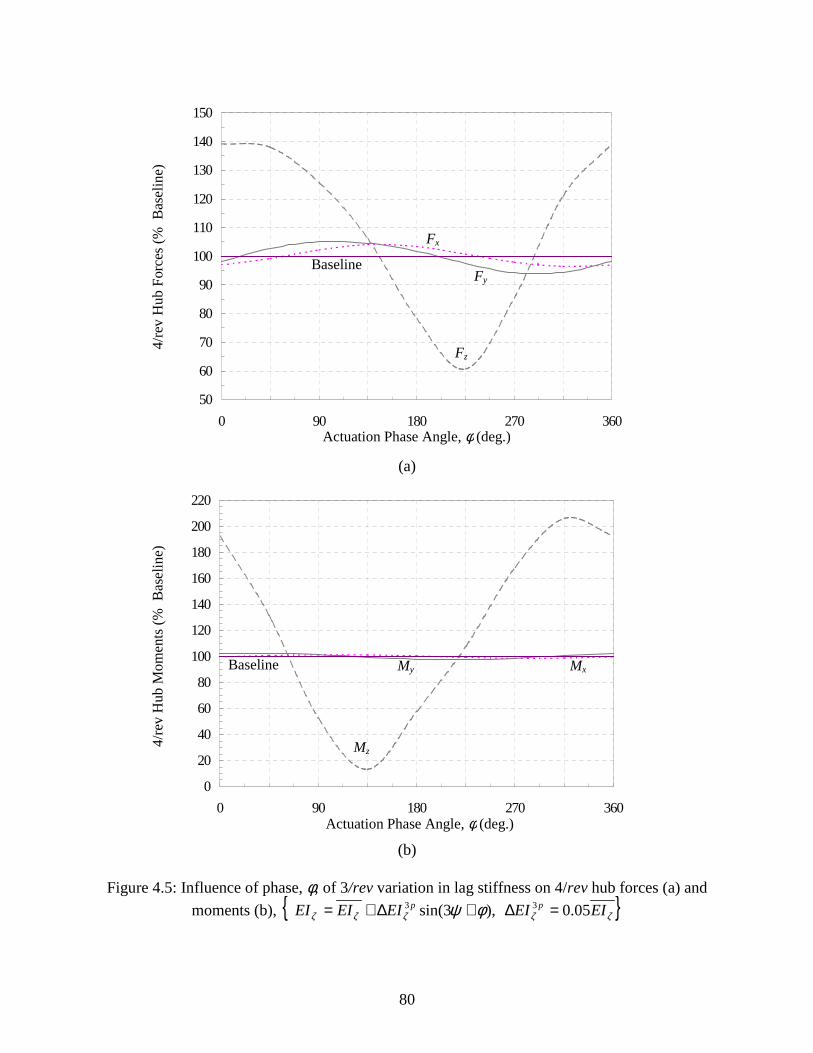
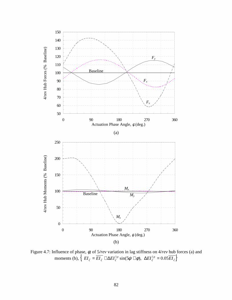
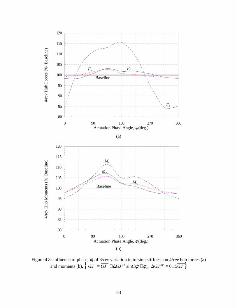
4.1 Influence of root element stiffness variations on vibratory hub loads ………..…...644.1.1 Cyclic variation in flap stiffness ………………………………….…...……..644.1.2 Cyclic variation in lag stiffness ……………………………………………...664.1.3 Cyclic variation in torsion stiffness ………………………………………….684.1.4 Summary of beneficial root element stiffness variations ……………………68

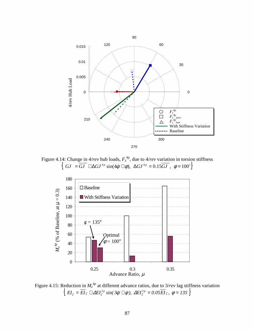
4.2 Mechanism for reduction of vibratory hub loads……………………….………….694.3 Influence of root element stiffness variation on blade root loads……...………..…71

4.3.1 Cyclic variation in flap stiffness ………………………………………...…...724.3.2 Cyclic variation in lag stiffness ……………………………………………...724.3.3 Cyclic variation in torsion stiffness ……………………………………….....74

4.4 Vibration reduction at different advance ratio ..…….……………..………………744.5 Summary on sensitivity of root element stiffness variation ..…………...…………75

Chapter 5 Optimal Control Study ……………………………………………….………….92

5.1 Optimal 3/rev flap stiffness variation …………………………………..……..…...925.2 Optimal 2,3/rev flap & 3/rev lag stiffness variations……………………….……….935.3 Optimal 2,3/rev Flap & Lag Stiffness Variations……...………………….……..…935.4 Influence of Baseline Stiffness on Effectiveness of Vibration Control ..…….….…945.5 Effectiveness of Vibration Controller at Different Forward Speed ..………………965.6 Summary on optimal control of root element stiffness variation..…………………96

Chapter 6 Discrete Controllable Stiffness Devices ………….…………………………….104

6.1 Baseline configuration ………………………………………………...……..…...1046.2 Optimal 2,3/rev flap stiffness variations………………………………….……….1056.3 Optimal 2,3/rev lag stiffness variations ……...………………………….……..…1056.4 Optimal 3,4/rev torsion stiffness variations…………………………...…….….…1056.5 Optimal 2,3/rev flap and lag stiffness variations ..……………………………...…1066.6 Influence of flexure stiffness on effectiveness of vibration control..…………..…1066.7 Effectiveness of vibration controller at different forward speed ..……………..…1076.8 Summary on discrete controllable stiffness device..…………………………...…107

Chapter 7 Discrete Controllable Stiffness Device Results – Model Refinements……...….115

7.1 Baseline configuration ………………………………………………...……..…...1157.2 Optimal 2,3/rev flap device stiffness variations …………….………………....….1167.3 Optimal 2,3/rev lag device stiffness variations …………...………………………1167.4 Optimal 3,4/rev torsion device stiffness variations ………………………………1177.5 Optimal 2,3/rev flap and lag device stiffness variations ..…………….………..…1187.6 Influence of flexure stiffness on effectiveness of vibration control ..………….…1187.7 Effectiveness of vibration controller at different forward speeds .…………….…1197.8 Summary on effectiveness of discrete controllable stiffness device ..……………119

vii

Chapter 8 Discrete Controllable Orifice Dampers………………………………...……….129

8.1 Baseline configuration………………………………………………………..…...1298.2 Lag Damping Variation ……………………….………………………………….130

8.2.1 Influence of optimal 2,3/rev lag damping variations……………….………1308.2.2 Influence of lag damper sizing and configuration …………………..……...133

8.3 Simultaneous flap and lag damping variations ..…….……………..………..……1358.3.1 Influence of optimal 2,3/rev flap and lag damping variations………………1358.3.2 Effectiveness of flap and lag damping variations at different flight speeds ..138

8.4 Summary on controllable orifice dampers ..…………………………....…………138

Chapter 9 Semi-Active Isolator ………………………………………………….….….….153

9.1 System description…………………………………………………………...…...1539.1.1 System with controllable stiffness device……………….…………….……1549.1.2 System with controllable damper…………………………………………...154

9.2 Fundamentals of Controller Design……………………….………………..…….1559.2.1 Optimal semi-active control scheme……………….………………….……1559.2.2 Semi-active device saturation consideration ………………………..……...1569.2.3 Frequency content of the semi-active input………………………...………1579.2.4 Identification of the system transfer matrix, T……………………....……...158

9.3 Semi-active controller schemes..…….……………..………………………..……1609.3.1 Open-loop controller……………………………………………..…………1609.3.2 Closed-loop controller……………………………………………………....1609.3.3 Closed-loop adaptive controller……………………………………...……..161

9.4 Effectiveness of semi-active controllers for vibration reduction..…….……….…1619.4.1 Baseline System………………………………………………………….…1619.4.2 Vibration reduction using open-loop controller……………………….……162

9.4.2.1 Controllable stiffness device………………………………....…1629.4.2.2 Controllable damper…………………………………..……...…164

9.4.3 Vibration reduction using closed-loop controller…………………...………1649.4.3.1 Closed-loop controller with controllable stiffness device…....…1659.4.3.2 Closed-loop controller with controllable damper…………….…166

9.4.4 Closed-Loop Adaptive Control Scheme……………………………….……1669.5 Summary of semi-active isolator ..………………………………………….....…167

Chapter 10 Concluding Remarks and Recommendations…….………………………….….179

10.1 Concluding remarks………………………………………………….…………...17910.2 Recommendations for future work …………………………………….…….…...182

References………………..…………………………………….………………………….….184

Appendix A Loads on Helicopter Fuselage………………………………….…….……….195

A.1 Loads from fuselage………………………………………….………..……..…...195A.2 Lift from horizontal tail………………………………………….……….……….195A.3 Thrust from tail rotor ……...………………………………………….………..…196

viii

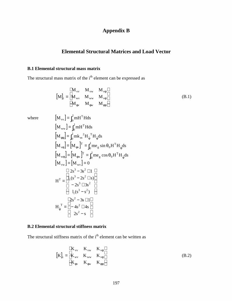
Appendix B Elemental Structural Matrices and Load Vector…..………………………….197

B.1 Elemental structural mass matrix………………………….……………………...197B.2 Elemental structural stiffness matrix…………………………….……….……….197B.3 Elemental structural damping matrix……...………………..………………….…198B.4 Elemental structural force vector……...…………………….……………………198

Appendix C Rotor Inflow Models ……………………………………….….…….……….200

C.1 Linear inflow model…………………………………….……………..……..…...200C.2 Rotor inflow using free wake analysis………………………………………...….200

Appendix D Elemental Aerodynamic Load Vector…..…………………………………….201

D.1 Resultant incident velocity………………………….………………..…………...201D.2 Blade sectional loads from circulatory effects..………………………….……….201D.3 Blade sectional loads from non-circulatory effects ...…...…….…………….……202D.4 Elemental aerodynamic force vector ……...……………………..…….…………202

Appendix E Blade Response Calculation …..………………...……………………………203

Appendix F Vehicle Trim Calculation…..…………………...…………………………….205

Appendix G Fluid Dynamic Model of Controllable Damper…..……………………….….206

Appendix H Helicopter and Rotor Properties…..……………………………………….….207

Appendix I Convergence Study: Numbers of Finite Elements and Modal Representation.208

I.1 Number of finite elements along the blade span………………...………………..208I.2 Number of blade modes in modal transformation ……………….……………….209

ix

LIST OF TABLES

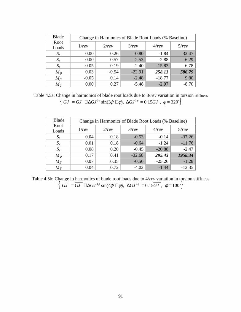
Table 4.1a: 4/rev vibratory hub loads for baseline rotor, no root element stiffness variation ..88

Table 4.1b: Harmonics of blade root loads for baseline rotor, no root elementstiffness variation………………………………………………………………...88

Table 4.2: Summary of beneficial effects of stiffness variations on vibratory hub loads…...88

Table 4.3a: Change in harmonics of blade root loads due to 2/rev variation in flap

stiffness o240,15.0),2sin( 22 ==∆+∆+= φφψ βββββ EIEIEIEIEI pp ….....89

Table 4.3b: Change in harmonics of blade root loads due to 3/rev variation in flap

stiffness o45,15.0),3sin( 33 ==∆+∆+= φφψ βββββ EIEIEIEIEI pp ……....89

Table 4.4a: Change in harmonics of blade root loads due to 2/rev variation in lag

stiffness o90,15.0),2sin( 22 ==∆+∆+= φφψ ζζζζζ EIEIEIEIEI pp ………89

Table 4.4b: Change in harmonics of blade root loads due to 3/rev variation in lag

stiffness o135,05.0),3sin( 33 ==∆+∆+= φφψ ζζζζζ EIEIEIEIEI pp ……...90

Table 4.4c: Change in harmonics of blade root loads due to 3/rev variation in lag

stiffness o225,05.0),3sin( 33 ==∆+∆+= φφψ ζζζζζ EIEIEIEIEI pp …......90

Table 4.4d: Change in harmonics of blade root loads due to 5/rev variation in lag

stiffness o200,05.0),5sin( 55 ==∆+∆+= φφψ ζζζζζ EIEIEIEIEI pp ……...90

Table 4.5a: Change in harmonics of blade root loads due to 3/rev variation in torsion

stiffness o320,15.0),3sin( 33 ==∆+∆+= φφψ GJGJGJGJGJ pp ……...91

Table 4.5b: Change in harmonics of blade root loads due to 4/rev variation in torsion

stiffness o100,15.0),4sin( 44 ==∆+∆+= φφψ GJGJGJGJGJ pp …...91

Table 5.1: Change in harmonics of blade root loads due to optimal 3/rev flapstiffness variation……………………………………………………………….102

Table 5.2: Optimal 2, 3/rev flap and 3/rev lag stiffness variations (Jz = 8.92)……………..102

Table 5.3a: Optimal 2, 3/rev flap and lag stiffness variations using gradient basedoptimization, without input penalty (Wk = 0), (Jz = 7.34)………………..……..102

Table 5.3b: Optimal 2, 3/rev flap and lag stiffness variations using non-gradient basedoptimization, without input penalty (Wk = 0), (Jz = 3.55)………………..……..103

Table 5.3c: Optimal 2, 3/rev flap and lag stiffness variations using gradient basedoptimization with input penalty (Wk = I)………………………………....……..103

Table 5.4: Change in harmonic of blade root loads due to the optimal 2,3/rev flap and lagstiffness variation (Wk = I)…………………...………………………………….103

x

Table 6.1: Discrete controllable stiffness device and blade flexure properties………….....112

Table 6.2a: 4/rev vibratory hub loads for baseline rotor - no stiffness variation(Drees inflow, µ = 0.3)…………………...………………………………….….112

Table 6.2b: Harmonics of blade root loads for baseline rotor - no stiffness variation(Drees inflow, µ = 0.3)…………………...………………………………….….112

Table 6.2c: 4/rev vibratory hub loads for baseline rotor -no stiffness variation(Drees inflow, µ = 0.35)…………………...…………………………..…….….113

Table 6.2d: Harmonics of blade root loads for baseline rotor - no stiffness variation(Drees inflow, µ = 0.35)…………………...………………………..……….….113

Table 6.3: Optimal 2, 3/rev flap device stiffness variations (Jz = 24.2)……………...….....113

Table 6.4: Optimal 2, 3/rev lag device stiffness variations (Jz = 60.8)………….…...….....113

Table 6.5: Optimal 2, 3/rev torsion device stiffness variations (Jz = 91.3)…………..….....114

Table 6.6: Optimal 2, 3/rev flap and lag device stiffness variations (Jz = 14.28)……….....114

Table 6.7: Change in harmonics of blade root loads due to the optimal 2,3/rev flap and lagspring stiffness variations …………………...………………………………….114

Table 7.1: Discrete controllable stiffness device and blade flexure properties………….....126

Table 7.2a: 4/rev vibratory hub loads for baseline rotor – no cyclic stiffness variation(Free-wake, µ = 0.3)…………………...…………………………………….….126

Table 7.2b: Harmonics of blade root loads for baseline rotor – no cyclic stiffness variation(Free-wake, µ = 0.3)…………………...…………………………………….….126

Table 7.3: Optimal 2,3/rev flap device stiffness variations (Jz = 69.25)…………….…......127

Table 7.4: Optimal 2,3/rev lag device stiffness variations (Jz = 84.23)…………….….......127

Table 7.5: Optimal 3,4/rev torsion spring stiffness variations, with varying input

weights (Wu) and baseline torsion spring stiffness (φK and 2 φK )………….….127

Table 7.6: Optimal 2,3/rev flap and lag devices stiffness variations (Jz = 67.23)……….....128

Table 7.7: Change in harmonics of blade root loads due to the optimal 2,3/rev flap and lagdevice stiffness variations…………………...………………………………….128

Table 8.1: Discrete controllable damper properties and blade frequencies…………..….....149

Table 8.2a: 4/rev vibratory hub loads for baseline rotor, no cyclic damping variation……..149

Table 8.2b: Harmonics of blade root loads for baseline rotor, no cyclic damping variation..149

Table 8.2c: Harmonics of flexbeam root loads for baseline rotor, no cyclicdamping variation…………………………………………………………...…..149

Table 8.2d: Harmonics of damper loads for baseline rotor, no cyclic damping variation..…150

xi

Table 8.2e: Harmonics of blade tip response for baseline rotor, no cyclicdamping variation …………………………………………………………..…..150

Table 8.3: Optimal 2,3/rev lag damping variation (Jz = 64.55) ……………….…….…......150

Table 8.4: Change in harmonics of damper loads, due to optimallag damping variation (from Table 8.3)……………………………..………….150

Table 8.5: Change in harmonics of blade root loads, due to optimallag damping variation (from Table 8.3)……………………………..………….151

Table 8.6: Change in harmonics of flexbeam root loads, due to optimallag damping variation (from Table 8.3)……………………………..………….151

Table 8.7: Change in harmonics of blade tip lag response, due to optimallag damping variation (from Table 8.3)……………………………..………….151

Table 8.8: Optimal 2, 3/rev flap and lag damping variations (Jz = 52.87)……….….…......151

Table 8.9: Change in harmonics of damper loads, due to optimalflap and lag damping variations (from Table 8.8)………………...…………….152

Table 8.10: Change in harmonics of blade root loads, due to optimalflap and lag damping variations (from Table 8.8)…………………...………….152

Table 8.11: Change in harmonics of flexbeam root loads, due to optimalflap and lag damping variations (from Table 8.8)………………...…………….152

Table 8.12: Change in harmonics of blade tip flap and lag responses, due to optimalflap and lag damping variations (from Table 8.8)………...…………………….152

Table 9.1: Numerical values of system parameters for single degree of freedom system....178

Table H.1: Rotor and fuselage properties…………………………………...….…….…......207

Table I.1: Optimal stiffness variations predicted using 2 flap, 2 lag, and 2 torsion modes(Drees inflow, µ = 0.35)………………………………...………...…………….215

Table I.2: 4/rev vibratory hub loads (predicted using 2 flap, 2 lag, and 2 torsion modes),with and without stiffness variations (Drees inflow, µ = 0.35)……………...….215

xii

LIST OF FIGURES

Figure 1.1: Helicopter vibration profile at various forward speeds………………..……….22

Figure 1.2: Blade Vortex Interaction (BVI) schematic…………………….……..………...22

Figure 1.3: Angle of attack variation at a high-speed forward flight ………………..……..22

Figure 1.4: Frequency analysis of normalized vibration of a four-bladed helicopter in (a) the blade [rotating frame] and (b) the fuselage [non-rotating frame]…...23

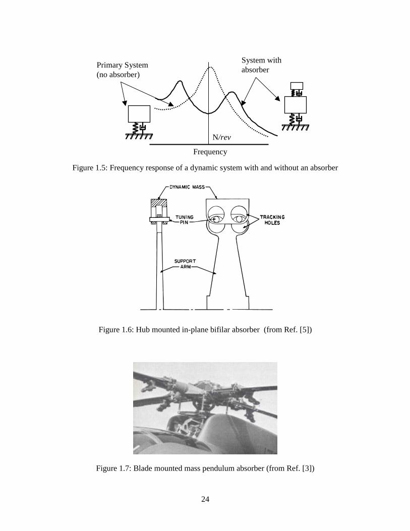
Figure 1.5: Frequency response of a dynamic system with and without an absorber….…..24

Figure 1.6: Hub mounted in-plane bifilar absorber……………………………………..….24

Figure 1.7: Blade mounted mass pendulum absorber …………………………………..….24

Figure 1.8: Helicopter vibration isolators; (a) Isolation platform with elastomericpads and (b) Nodal beam……………………………………………………….25

Figure 1.9: Schematic of a Higher Harmonic Control (HHC) system ……………………..25

Figure 1.10: Schemetics of Individual Blade Control (IBC) systems using(a) blade pitch, (b) active flap, and (c) blade twist controls……………..……..26

Figure 1.11: Schematics of Active Control of Structural Response (ACSR) systemsusing force actuators located in (a) engine platform and (b) cabin…………….27

Figure 1.12: Schematics of (a) a semi-active suspension model and(b) a semi-active controllable damper………………………………………….27

Figure 1.13: Schematics of (a) a building model for sesmic testing and (b) a semi-active controllable orifice damper, and (c) calibration curve of thecontrollable damper…………………………………………………………….28

Figure 1.14: Schematics of (a) a building model for sesmic testing and (b) a semi-active MR damper, and (c) MR damper characteristic…………………………29

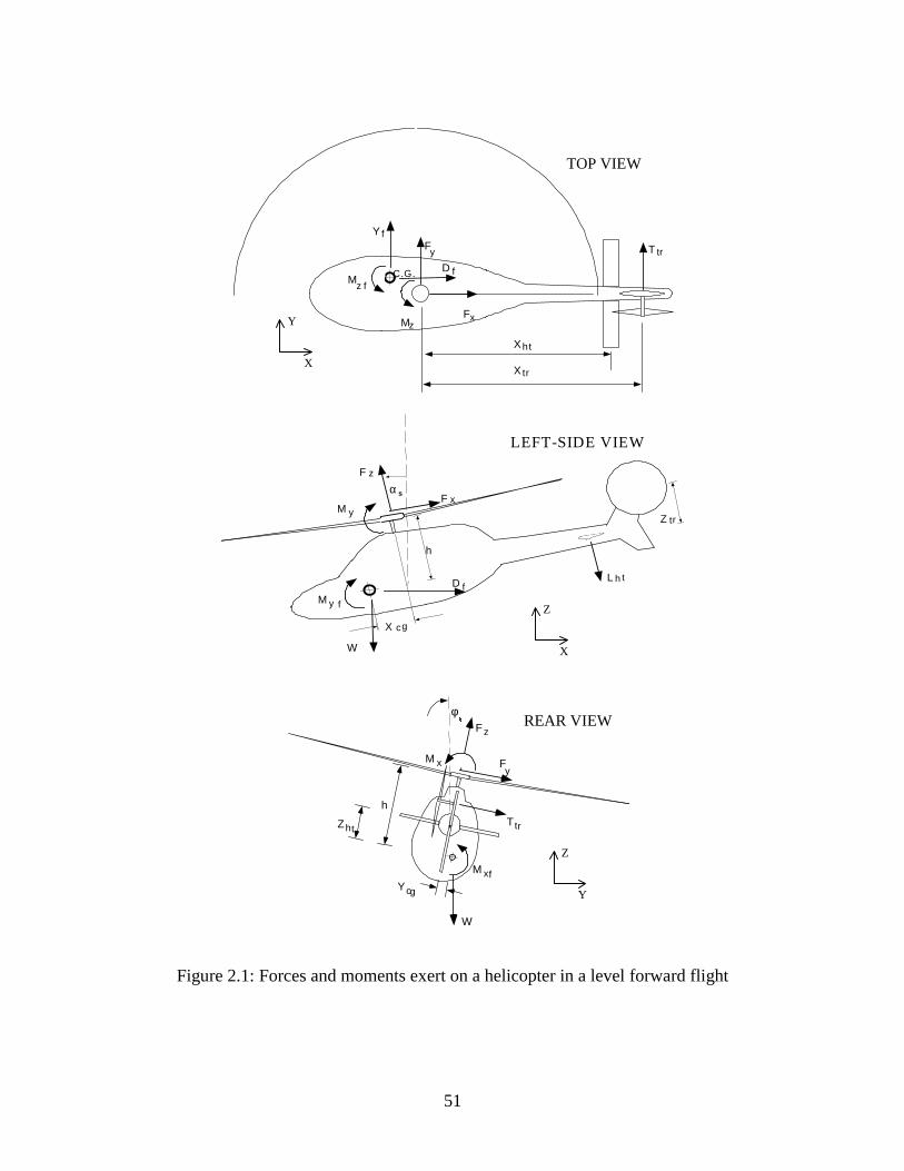
Figure 2.1: Forces and moments exert on a helicopter in a level forward flight…………...51

Figure 2.2: Spatial discretization of a rotor blade using Finite Element Method…………..52

Figure 2.3: Global mass matrix of a rotor blade with 5 spatial elements…………………..52

Figure 2.4: Discretization of azimuthal position for blade response calculationusing Finite Element in time method…………………………………………..52

Figure 2.5: Flowchart of coupled rotor/trim response calculation procedure………………53

Figure 2.6: Nodal blade shear forces in vertical and chordwise directions………………...54

Figure 2.7: Nodal blade moments in flapwise direction……………………………………54

Figure 2.8: Blade root shear forces and moments ………………………………………….54

Figure 2.9: Transformation between Hub loads and Blade Root Loads……………………55

xiii

Figure 2.10: Stiffness variation of the root element …………………………………………55

Figure 2.11: Schematic sketch of discrete controllable stiffness devices……………………55

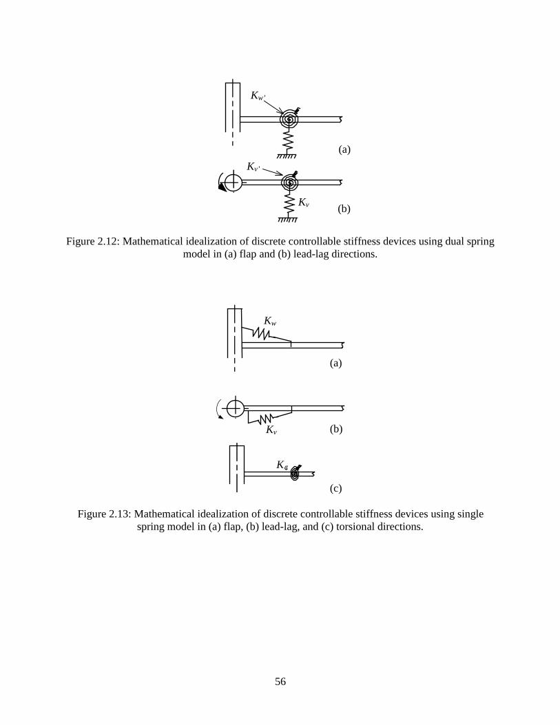
Figure 2.12: Mathematical idealization of discrete controllable stiffness devicesusing dual spring model in (a) flap and (b) lead-lag directions………………...56

Figure 2.13: Mathematical idealization of discrete controllable stiffness devices usingsingle spring model in (a) flap, (b) lead-lag, and (c) torsional directions……...56

Figure 2.14: Configuration and attachment geometry of controllable stiffness devices,(a) flap device and (b) lag device………………………………………………57

Figure 2.15: (a) Deformation of the flap device due to blade bending, and(b) Loads exerted on the blade at attachment point by the flap device………...57

Figure 2.16: Schematic of a semi-active controllable damper………………….……………58

Figure 2.17: Force/Displacement hysteresis loops for different bypass orifice settings(valve voltages); (a) experiment, (b) fluid dynamic model simulations(from Ref. 103)…………………………………………………………………58

Figure 2.18: Force/Displacement hysteresis cycles produced by the fluid dynamicsbased damper model and an equivalent damping coefficient model(at a specified orifice command voltage Vo)…………………………………...58

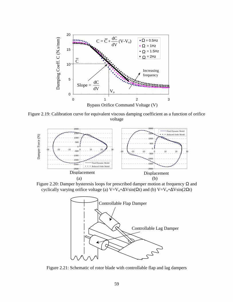
Figure 2.19: Calibration curve for equivalent viscous damping coefficient asa function of orifice voltage……………………………………………………59

Figure 2.20: Damper hysteresis loops for prescribed damper motion at frequency Ωand cyclically varying orifice voltage (a) V=Vo+∆Vsin(Ωt) and(b) V=Vo+∆Vsin(2Ωt) …………………………………………………………59

Figure 2.21: Schematic of rotor blade with controllable flap and lag dampers……………...59

Figure 2.22: (a) Deformation of the flap damper due to blade bending, and(b) loads exerted on the blade at attachment point by the flap damper ………..60

Figure 2.23a: Blade root vertical shear, Sz, with contributions from the flexbeam,Sz

flex (obtained by summing vertical shear forces, fzi, along blade

Finite Element DOF’s), and the flap damper, Szdamper …………………………60

Figure 2.23b: Blade root drag shear, Sx, with contributions from the flexbeam, Sxflex

(obtained by summing drag shear forces, fxi, along blade Finite Element

DOF’s), and the lag damper, Sxdamper …………………………………………..60

Figure 4.1: Influence of phase, φ, of 1/rev variation in flap stiffness on 4/rev hub forces

(a) and moments (b), βββββ φψ EIEIEIEIEI pp 15.0),sin( 11 =∆+∆+= .….76


(a) and moments (b), βββββ φψ EIEIEIEIEI pp 15.0),2sin( 22 =∆+∆+= ...77

xiv


(a) and moments (b), βββββ φψ EIEIEIEIEI pp 15.0),3sin( 33 =∆+∆+= …78

Figure 4.4: Influence of phase, φ, of 2/rev variation in lag stiffness on 4/rev hub forces

(a) and moments (b), ζζζζζ φψ EIEIEIEIEI pp 15.0),2sin( 22 =∆+∆+= …79


(a) and moments (b), ζζζζζ φψ EIEIEIEIEI pp 05.0),3sin( 33 =∆+∆+= ….80

Figure 4.6a: Influence of magnitude of 3/rev variations in lag stiffness on vibratory hub torque………………………………………………………………………81

Figure 4.6b: Influence of magnitude of lag stiffness variations on vibratory hub torque…...81


(a) and moments (b), ζζζζζ φψ EIEIEIEIEI pp 05.0),5sin( 55 =∆+∆+= …82

Figure 4.8: Influence of phase, φ, of 3/rev variation in torsion stiffness on 4/rev hub forces

(a) and moments (b), GJGJGJGJGJ pp 15.0),3sin( 33 =∆+∆+= φψ ..83

Figure 4.9: Influence of phase, φ, of 4/rev variation in torsion stiffness on 4/rev hub forces

(a) and moments (b), GJGJGJGJGJ pp 15.0),4sin( 44 =∆+∆+= φψ ..84

Figure 4.10: Change in 4/rev hub loads, Fz4p, due to 2/rev variation in flap stiffness

o240,15.0),2sin( 22 ==∆+∆+= φφψ βββββ EIEIEIEIEI pp ………………85

Figure 4.11: Change in contributions of hub load, Fx4p, due to 3/rev variation in flap


Figure 4.12: Change in 4/rev hub loads, Fz4p, due to due to 3/rev variation in flap


Figure 4.13: Change in 4/rev hub loads, Fz4p, due to 3/rev variation in lag stiffness

o225,05.0),3sin( 33 ==∆+∆+= φφψ ζζζζζ EIEIEIEIEI pp ……………..86

Figure 4.14: Change in 4/rev hub loads, Fz4p, due to 4/rev variation in torsion stiffness

o100,15.0),4sin( 44 ==∆+∆+= φφψ GJGJGJGJGJ pp …………...87

Figure 4.15: Reduction in Mz4p at different advance ratios, due to 3/rev lag stiffness

variation o135,05.0),3sin( 33 ==∆+∆+= φφψ ζζζζζ EIEIEIEIEI pp ….87

Figure 5.1: Contour plot of performance index, J, (% Baseline)due to 3/rev flap stiffness variation…………………………………………….97

Figure 5.2: Hub vibration reduction due to optimal 3/rev flap stiffness variation………....97

xv

Figure 5.3: Hub vibration reduction due to optimal 2,3/rev flap and 3/rev lagstiffness variations.……………………………………………………………..98

Figure 5.4: Hub vibration reduction due to optimal 2,3/rev flap and lag stiffness variations with gradient based (G) and non-gradient based (NG) optimizations …………98

Figure 5.5: Hub vibration reduction due to optimal 2,3/rev flap and lag stiffnessvariations with (Wu = I) and without (Wu = 0) input penalty…………………...99

Figure 5.6: Effectiveness of optimal 2,3/rev flap and lag stiffness variations fordifferent values of blade flap stiffness (flap natural frequency)……………….99

Figure 5.7: Effectiveness of optimal 2,3/rev flap and lag stiffness variations fordifferent values of blade lag stiffness (lag natural frequency)………………..100

Figure 5.8: Effectiveness of optimal 2,3/rev flap and lag stiffness variations fordifferent values of blade torsion stiffness (torsion natural frequency)….…….100

Figure 5.9: Effectiveness of optimal 2,3/rev flap and lag stiffness variations for different advance ratios……………………………………………………….101

Figure 6.1: Hub vibration reduction due to optimal 2,3/rev discrete flapstiffness variations…………………………………………………………….108

Figure 6.2: Hub vibration reduction due to optimal 2,3/rev discrete lagstiffness variations…………………………………………………………….108

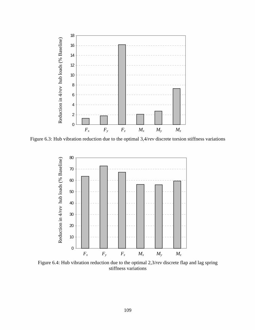
Figure 6.3: Hub vibration reduction due to the optimal 3,4/rev discrete torsion stiffness variations…………………………………………………….109

Figure 6.4: Hub vibration reduction due to the optimal 2,3/rev discreteflap and lag spring stiffness variations………………………………………..109

Figure 6.5: Effectiveness of optimal 2,3/rev discrete flap and lag springstiffness variations for different value of flap flexure stiffness ………………110

Figure 6.6: Effectiveness of optimal 2,3/rev discrete flap and lag springstiffness variations for different value of lag flexure stiffness………………..110

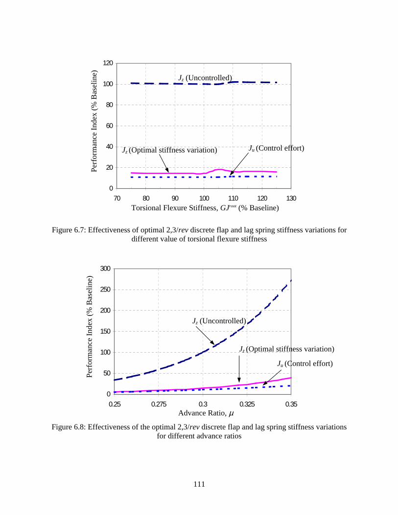
Figure 6.7: Effectiveness of optimal 2,3/rev discrete flap and lag spring stiffness variations for different value of torsional flexure stiffness………….111

Figure 6.8: Effectiveness of the optimal 2,3/rev discrete flap and lag spring stiffness variations for different advance ratios………………………………111

Figure 7.1: Hub vibration reduction due to optimal 2,3/rev flap devicestiffness variations…………………………………………………………….121

Figure 7.2: Optimal flap device stiffness variation over one rotor revolution,(with 2, 3/rev inputs from Table 7.3)…………………………………………121

Figure 7.3: Hub vibration reduction due to optimal 2,3/rev lag devicestiffness variations…………………………………………………………….122

xvi

Figure 7.4: Hub vibration reduction due to optimal 3,4/rev torsion device stiffness

variations (Wu = 0.02[I], baseline torsion device stiffness = φK )……………122

Figure 7.5: Hub vibration reduction due to the optimal 3,4/rev torsion device stiffness variations, with varying input weights (Wu) and baseline torsion spring

stiffness ( φK ,2 φK )…………………………………………………………...123

Figure 7.6: Hub vibration reduction due to optimal 2,3/rev flap and lag device stiffness variations…………………………………………………………….123

Figure 7.7: Effectiveness of optimal 2,3/rev flap and lag device stiffness variations for different values of flap flexure stiffness…………………………………..124

Figure 7.8: Effectiveness of optimal 2,3/rev flap and lag device stiffness variations for different values of lag flexure stiffness…………………………………...124

Figure 7.9: Effectiveness of optimal 2,3/rev flap and lag device stiffness variations for different values of torsion flexure stiffness……………………………….125

Figure 7.10: Effectiveness of optimal 2,3/rev flap and lag device stiffness variations for different advance ratios……………………………………………………125

Figure 8.1: Optimal lag damping variation over one rotor revolution(with 2/rev and 3/rev inputs from Table 8.3)…………………………………139

Figure 8.2: Hub vibration reduction due to optimal 2, 3/rev lag damping variation……...139

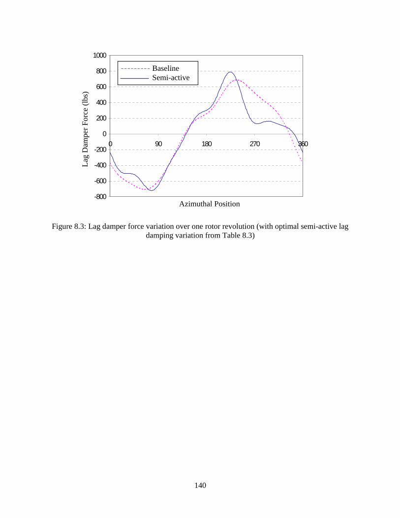
Figure 8.3: Lag damper force variation over one rotor revolution (with optimal semi-active lag damping variation from Table 8.3)…………………………..140

Figure 8.4: Blade root loads over one rotor revolution (with optimal semi-active lagdamping variation from Table 3), (a) blade root drag shear, Sx, and(b) blade root radial shear, Sr………………………………………………….141

Figure 8.5: Flexbeam root loads over one rotor revolution (with optimal semi-active lag damping variation from Table 8.3), (a) flexbeam root drag shear, Sx

flex,and (b) flexbeam root radial shear, Sr

flex………………………………………142

Figure 8.6: Blade flap, lag, and torsional tip responses over one rotor revolution(with optimal semi-active lag damping variation from Table 8.3) …………...143

Figure 8.7: Effectiveness of lag damping variation in reducing vibration fordifferent damper mounting angles…………………………………………….143

Figure 8.8: Effectiveness of lag damping variation in reducing vibration fordifferent damper offsets ………………………………………………………144

Figure 8.9: Effectiveness of lag damping variation in reducing vibration fordifferent damper attachment points…………………………………………...144

Figure 8.10: Effectiveness of lag damping variation in reducing vibration fordifferent damper sizes…………………………………………………………145

xvii

Figure 8.11: Optimal flap and lag damping variations over one rotor revolution(with 2/rev and 3/rev inputs from Table 8.8)…………………………………145

Figure 8.12: Hub vibration reduction due to optimal 2, 3/rev flap and lagdamping variations……………………………………………………………146

Figure 8.13: Lag damper force variation over one rotor revolution (with optimalsemi-active flap and lag damping variations from Table 8.8)………………...146

Figure 8.14: Flap damper force variation over one rotor revolution (with optimal semi-active flap and lag damping variations from Table 8.8)………………...147

Figure 8.15: Blade flap, lag, and torsional tip responses over one rotor revolution(with optimal semi-active flap and lag damping variations from Table 8.8)…147

Figure 8.16: Effectiveness of optimal 2, 3/rev flap and lag damping variationsfor different advance ratios……………………………………………………148

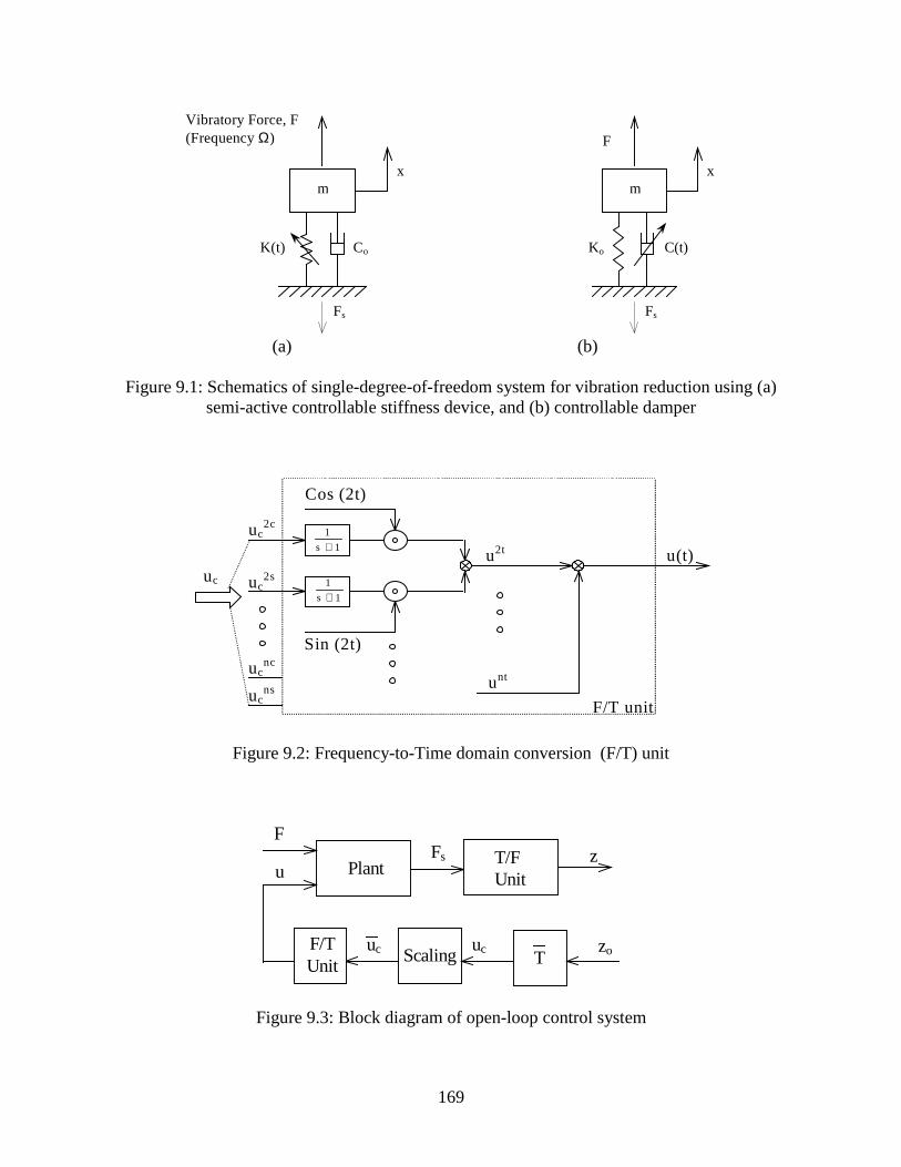
Figure 9.1: Schematics of single-degree-of-freedom system for vibration reduction using (a) semi-active controllable stiffness device, and (b) controllable damper…..169

Figure 9.2: Frequency-to-Time domain conversion (F/T) unit…………………………...169

Figure 9.3: Block diagram of open-loop control system……………………………..…...169

Figure 9.4: Block diagram of closed-loop control system………………………………...170

Figure 9.5: Block diagram of closed-loop adaptive control system…………………….....170

Figure 9.6: (a) Time history and (b) corresponding frequency content of disturbanceforce, F, and support force, Fs, of the baseline uncontrolled system…………171

Figure 9.7: Frequency content of disturbance force, F, and support force, Fs,due to optimal stiffness variation input (no input limits)……………………..172

Figure 9.8: Frequency content of disturbance force, F, and support force, Fs,due to optimal semi-active stiffness variation (input “scaled-down”)………..172

Figure 9.9: Frequency contents of support force, Fs, for increasing stiffness variation input amplitudes.……………………………………………………173

Figure 9.10: Frequency contents of support force, Fs, for increasing semi-activedamping variation input amplitudes (with “input scaling”).………………….173

Figure 9.11: Time history of disturbance force, F, and support force, Fs, for closed-loop controller with controllable stiffness device,

with change in phase of excitation force (φ = 45°)…………………………..174

Figure 9.12: Amplitude of support force, Fs, at disturbance frequency, Ω, for open-loop and closed-loop controller with controllable stiffness device, with change in phase of excitation force (φ = 45°)…………………..174

Figure 9.13: Amplitude of support force, Fs, at excitation frequency, Ω, for open-loop and closed-loop controllers with controllable stiffness device, with change in phase of excitation force (φ = 90°)…………………..175

xviii

Figure 9.14: Variation in steady state support force, Fs, at Ω for closed-loop and open-loop controllers with controllable stiffness device as a function of change in phase of excitation force……………………………..175

Figure 9.15: Variation in steady state support force, Fs, at Ω for closed-loop and open-loop controllers with controllable damper as a function of change in phase of excitation force……………………………..176

Figure 9.16: Amplitude of support force, Fs, at excitation frequency, Ω, for closed-loop adaptive controller using controllable stiffness device, with change in phase of excitation force (φ = 45°)…………………………..176

Figure 9.17: Amplitude of support force, Fs, at excitation frequency, Ω, for closed-loop adaptive controller using controllable stiffness device, with change in phase of excitation force (φ = 90°)…………………………..177

Figure 9.18: Variation in steady state support force, Fs, at Ω for open-loop, closed-loop and closed-loop adaptive controllers with controllable stiffness device as a function of change in phase of excitation force…………177

Figure I.1: Rotor blade finite element discretization used in the convergence study…….211

Figure I.2: Blade rotating natural frequencies for increasing number of finite elements...211

Figure I.3: Blade flap mode shapes for increasing number of finite elements …………...212

Figure I.4: Blade lag mode shapes for increasing number of finite elements…………….212

Figure I.5: Blade torsional mode shapes for increasing number of finite elements………213

Figure I.6: Variation in 4/rev vibratory hub load predictions with increasing number of flap modes, when a 2,3/rev flap stiffness variation is used

(Drees inflow, µ = 0.35)………………………………………………………213

Figure I.7: Variation in 4/rev vibratory hub load predictions with increasing number of lag modes, when a 2,3/rev lag stiffness variation is used

(Drees inflow, µ = 0.35)………………………………………………………214

Figure I.8: Variation in 4/rev vibratory hub load predictions with increasing number of torsion modes, when a 3,4/rev torsion stiffness variation is used (Drees inflow, µ = 0.35)………………………………………………214

xix

LIST OF SYMBOLS

a Blade section lift-curve slope

aht Horizontal tail section lift-curve slope

atr Tail rotor blade section lift-curve slope

A Rotor disk area

Ap, Af, Ar Piston, accumulator, and rod area

Apri, Acon Primary and controllable orifice area

b Blade half chord

c Blade chord

C Damping matrix

[C]i Structural damping matrix of the ith element

Cvv, Cvw, Cvφ Damping matrix associated with lag degree of freedom

Cwv, Cww, Cwφ Damping matrix associated with flap degree of freedom

Cφv, Cφw, Cφφ Damping matrix associated with torsion degree of freedom

ctr Tail rotor blade chord

Cd Sectional drag coefficient

Cl Sectional lift coefficient

Cm Sectional pitching moment coefficient

CT Thrust coefficient

CTtr Tail rotor thrust coefficient

Cw , Cv Damping coefficient of controllable flap and lag dampers

Co Baseline damping coefficient of controllable damper

C1 Maximum damping variation of controllable damper

Cyf , Cmxf , Cmyf , Cmzf Fuselage side force, rolling, pitching, and yawing moment

coefficients

D Sectional drag

Df Fuselage drag

ed Chordwise offset of blade center-of mass (ahead of elastic

axis)

ew , ev offset of controllable flap, lag stiffness devices (dampers)

xx

eg Chordwise offset of aerodynamic center (behind elastic

axis)

EIy , EIz Blade flapwise, chordwise stiffness

EB1 , EB2 Section stiffness constants

EC1 Warping rigidity

EC2 Section warping constant

f Equivalent drag area of helicopter fuselage and hub

fx , fz Nodal blade drag, vertical force

F Force vector

FA Aerodynamic load vector

FA Blade axial force

FD Damper force

Fi Structural load vector of the ith element

Fv, Fw, Fφ Load vector associated with lag, flap, and torsion degree of

freedom, respectively

FvA, Fw

A, FφA Aerodynamic load vector associated with lag, flap, and

torsion degree of freedom, respectively

Fs Support force

Fo Excitation force

Fx , Fy , Fz Rotor drag, side, and vertical forces

G Controller gain

GJ Blade torsional stiffness

h Hub offset above center of gravity

H Spatial modeshape vector (flap and lag degree of freedoms)

Ht Temporal modeshape vector

φH Spatial modeshape vector (torsion degree of freedom)

J Jacobian matrix

Jz , Ju Vibration index and semi-active input index

km Blade cross sectional mass radius of gyration

km1 , km2 Blade cross sectional mass radius of gyration in the flap

and lag directions, respectively

xxi

kpri, kcon Primary and controllable orifice discharge coefficient

K Stiffness matrix

Ka Equivalent accumulator stiffness

[K]i Structural stiffness matrix of the ith element

Kw , Kv , Kφ Stiffness of controllable flap, lead-lag, and torsion stiffness

devices

Kvv, Kvw, Kvφ Stiffness matrix associated with lag degree of freedom

Kwv, Kww, Kwφ Stiffness matrix associated with flap degree of freedom

Kφv, Kφw, Kφφ Stiffness matrix associated with torsion degree of freedom

Ko Baseline stiffness of controllable stiffness device

K1 Maximum stiffness variation of controllable stiffness

device

l, li Element length

L Sectional lift

Lht Lift of horizontal tail

Lu, Lv, Lw Blade forces in undeformed frame

Lu, Lv, Lw Blade forces in deformed frame

LuA, Lv

A, LwA Blade forces in deformed frame including non-circulatory

effect

LwNC Non-circulatory blade lift

m Mass, blade mass per unit length

mo Elemental mass

mβ , mζ , mφ Nodal blade flap, lag, and torsional moment

M Mass matrix

[M]i Structural mass matrix of the ith element

Mx , My , Mz Rotor rolling, pitching moment and torque

Mxf , Myf , Mzf Fuselage aerodynamic rolling, pitching moment and torque

Mβ , Mζ , Mφ Blade root flapping, lead-lag, and pitching moment

Mvv, Mvw, Mvφ Mass matrix associated with lag degree of freedom

Mwv, Mww, Mwφ Mass matrix associated with flap degree of freedom

Mφv, Mφw, Mφφ Mass matrix associated with torsion degree of freedom

xxii

φM Blade pitching moment in deformed frame

AMφ

Blade pitching moment in deformed frame including non-

circulatory effect

NCMφ

Non-circulatory blade pitching moment

N Number of main rotor blades

Ntr Number of tail rotor blades

p Modal coordinates

P Pressure

q Normalized coordinates

r Radial position

R Rotor radius

Rtr Tail rotor radius

s Local coordinate of spatial element

S Blade nodal load vector

Sht Horizontal tail area

Sr , Sx , Sz Blade root radial, drag, and vertical shear force

t Time, non-dimensional time

T Rotor thrust

Ttr Tail rotor thrust

TDU Transformation matrix from blade undeformed from to

blade deformed frame

u control input

uc control input (frequency domain)

U Section resultant velocity

UP, UR, UT Air velocity of blade; perpendicular, radial, tangential

components

Ux, Uy, Uz x, y, z components of blade sectional velocity

V Helicopter forward velocity

W Helicopter gross weight,

Wz, Wu Vibration and input penalty weighting matrix

xxiii

x Blade non-dimensional radial coordinate; body-fixed

coordinate; displacement

xcg Hub offset from center of gravity in x direction

xht Horizontal tail offset from center of gravity in x direction

xtr Tail rotor offset from center of gravity in x direction

y body-fixed coordinate, state vector

ycg Hub offset from center of gravity in y direction

Yf Fuselage aerodynamic side force

z body-fixed coordinate

ztr Tail rotor offset from center of gravity in z direction

α Blade section angle of attack

αs Longitudinal shaft tilt

αw , αv Mounting angle of controllable flap and lag stiffness device

(dampers)

β Fluid bulk modulus

βp Blade precone angle

δT Variational kinetic energy

δU Variational strain energy

δT Virtual work

δΠ Variational Hamiltonian

ε Error

γ Blade lock number

γtr Tail rotor blade lock number

η Solution vector for helicopter trim

ηr Distance from blade elastic axis to blade ¾ chord

θ Pitch angle

θo, θ1c, θ1s Collective, cosine, and sine components of blade pitch

θtr Tail rotor collective

λ Main rotor inflow ratio

λi Induced inflow

xxiv

λtr Tail rotor inflow ratio

λo Main rotor mean induced velocity

λ1c Cosine component of rotor inflow

λ1s Sine component of rotor inflow

µ Main rotor advance ratio

µtr Tail rotor advance ratio

ρ Air density

σ Rotor solidity

φ Section inflow angle; phase angle

Φ Eigenvectors representing mode shapes

φs Lateral shaft tilt

ψ Azimuth position

Main rotor rotational speed; excitation frequency

tr Tail rotor rotational speed

(•

) t∂∂ )(

( )’ x∂∂ )(

xxv

ACKNOWLEDGEMENTS

I would like to express my sincere appreciation to my advisor, Dr. Farhan Gandhi, who has

dedicated his years to teach and assist me in almost every aspect of life throughout my graduate

study. I am also grateful to members of my advisory committee, Drs. Smith, Lesieutre, and

Rahn, all of whom have shown interest in this work and provided countless advice and

discussion. I would like to thank Dr. Lane Miller of Lord Corp. for his valuable guidance and

suggestions.

The financial support for this research, which is provided by the Department of Aerospace

Engineering and the Rotorcraft Center of Excellence, is gratefully acknowledged. I am thankful

for the RCOE for awarding me many years of the Rotorcraft Center fellowships that presented

me with both financial as well as moral support.

I am grateful for many of my colleagues at the Rotorcraft Center for their friendship, support,

and help over the years. In particular, I appreciate Martin Sekula, Eric Hathaway, and Brendon

Malovrh for shearing their life, numerous stories, and laughter while we had some spare time

mostly on friday afternoon. Thanks also to Lionel Tauszig for his dedicated assistance with a

free wake analysis, which is used extensively in this research.

Most of all I am indebted to my parents, Viroj and Chumpee Anusonti-Inthra, half way around

the world for their unconditional love, support, and encouragement which guided me through the

years. I would like to express my gratitude to my brothers, Phurithat and Jackchai, who make

me feel loved and supported always. A special thank is dedicated to my future wife, Jirin

Palanuwech, for her kindness, care, and love.

1

Chapter 1

Introduction

1.1 Background and motivation

Helicopters play an essential role in today’s aviation with unique abilities to hover and take

off/land vertically. These capabilities enable helicopters to carry out many distinctive tasks in

civilian and military operations. Despite these attractive abilities, helicopter trips are usually

unpleasant for passengers and crew because of high vibration level in the cabin. This vibration is

also responsible for degradation in structural integrity as well as reduction in component fatigue

life. Furthermore, the high vibration environment may decrease the effectiveness of onboard

avionics or computer systems that are critical for aircraft primary control, navigation, and

weapon systems. Consequently, significant efforts have been devoted over the last several

decades for developing strategies to reduce helicopter vibration.

To develop a new helicopter vibration reduction method, it is essential to first understand the

origin and fundamental mechanics of helicopter vibration, which are summarized in Section 1.2.

A comprehensive review of previous helicopter vibration reduction schemes using both passive

and active strategies is also conducted and presented in Sections 1.3 and 1.4, respectively. This

suggests that passive vibration reduction concepts can produce modest performance (no power is

required), while incurring considerable weight penalty, and the designs are generally fixed with

no ability to adapt to any changes. Even though active vibration reduction methods can produce

relatively better performance and can adapt to changes in configuration or operating condition,

they usually require significant power to operate. This leads to an effort to combine the

advantages of passive and active vibration reduction strategies into a recently developed “semi-

active” approach, which is reviewed thoroughly in Section 1.5. Generally, the semi-active

method can produce better performance than purely passive approach, while using relatively

small power. However, most of the recent semi-active concepts are developed for broadband

2

vibration reduction applications, which are not directly applicable for helicopter use since

helicopter vibration is tonal or narrow-band in nature (helicopter vibration is concentrated at

some specific frequencies). This motivates the development of a new helicopter vibration

reduction scheme using the semi-active concept.

1.2 Overview of helicopter vibration

Helicopter vibration generally originates from many sources; for example, transmission, engine,

and tail rotor, but most of the vibration comes primarily from the main rotor system, even with a

perfectly tracked rotor. Figure 1.1, which shows a typical vibration profile of a helicopter, as a

function of cruise speeds, demonstrates that severe vibration usually occurs in two distinct flight

conditions; low speed transition flight and high-speed flight. In the low-speed transition flight

(generally during approach for landing), the severe vibration level is primarily due to impulsive

loads induced by interactions between rotor blades and strong tip vortices dominating the rotor

wake (see Fig. 1.2). This condition is usually referred to as Blade Vortex Interaction (BVI). In

moderate-to-high speed cruise, the BVI-induced vibration is reduced since vortices are washed

further downstream from the rotor blades, and the vibration is caused mainly by the unsteady

aerodynamic environment in which the rotor blades are operating. This highly periodic

aerodynamic environment creates large periodic variations in blade velocity and angle of attack,

and corresponding large periodic vibratory loads on the blades. Figure 1.3 shows, for example, a

typical variation in blade angle of attack around the azimuth for a high-speed forward flight. For

an extremely high-speed cruise, the vibration can be even more severe since the blades can

encounter shock on the advancing side (which generates large blade drag and pitching moment)

or stall on the retreating side (which results in sudden loss of lift) over every revolution. This

severe high vibration level and associated increases in rotor power generally limits the maximum

helicopter cruise speed.

Once the blade loads are generated, they are further transmitted into the non-rotating frame as

vibratory hub loads and then into the cabin as cabin vibration. Normally, sectional blade loads

are comprised of both aerodynamic and inertial contributions at harmonics of the rotor speed, Ω.

The aerodynamic component of blade loads is generated by periodic flow field around the

rotating blades, while the inertial component of blade loads is created by blade rotation

3

(gyroscopic effect) and blade motion in flap, lag and torsion directions. The sectional inertial

and aerodynamic blade loads can be integrated along the blade length to obtain the blade root

loads, also at harmonics of Ω, as seen in Fig. 1.4a. These blade root loads from every blade are

summed at the rotor hub to yield hub loads. Since the rotor blades are assumed identical,

implying identical blade root loads with the phase shifted properly, most of the harmonics of hub

loads will be filtered (cancelled) out, except components at the frequencies of; 0, NΩ, 2NΩ,

3NΩ, etc., where N is the number of blades, (see Fig. 1.4b). The most significant component of

the vibratory hub loads is the NΩ or N/rev component, and the amplitudes of the higher

harmonic are progressively smaller. These hub loads are then transmitted through the helicopter

cabin via the transmission platform. The amount of vibration throughout the helicopter cabin

may vary, depending on the vibration characteristics of the fuselage itself.

1.3 Passive helicopter vibration reduction

Passive strategies have been employed extensively for reducing helicopter vibration. Most of the

passive strategies produce moderate vibration reduction in certain flight conditions, and only at

some locations in the fuselage (such as, pilot seats or avionics compartments). The major

advantage of the passive concepts is that they require no external power to operate. However,

they generally involve a significant weight penalty and are fixed in design, implying no ability to

adjust to any possible change in operating conditions (such as changes in rotor RPM or aircraft

forward speed). Examples of these passive vibration reduction strategies include tuned-mass

absorbers, isolators, and blade design optimizations.

Tuned-mass vibration absorbers can be employed for reducing helicopter vibration both in the

fuselage and on the rotor system. The absorbers are generally designed using classical spring-

mass systems tuned to absorb energy at a specific frequency [1], for example at N/rev, thus

reducing system response or vibration at the tuned frequency (see Fig. 1.5). In the fuselage, the

absorbers are usually employed to reduce vibration levels at pilot seats or at locations where

sensitive equipment is placed. Without adding mass, an aircraft battery may be used as the mass

in the absorber assembly [2]. Vibration absorbers can also be integrated into the rotor hub system

(Fig. 1.6) or can be located on the blades themselves (Fig. 1.7). The absorbers are often designed

using a pendulum like configuration, with stiffness provided by centrifugal force. Various

4

configurations have been developed; for example blade-mounted vertical plane pendulum

absorbers [3], dual-frequency pendulum absorbers [4], hub-mounted inplane bifilar absorbers

[5], dual frequency monofilar inplane absorbers [6], and single-frequency inplane roller

absorbers [7]. Many design tradeoffs have to be considered when using these absorbers on

helicopters for vibration reduction. Generally a sizable absorber mass is required for a good

performance. Furthermore, the effectiveness of the absorbers is highly dependent on frequency,

thus changes in rotor RPM may even produce increases in the vibration levels. Also, some

power is lost due to the additional aerodynamic drag produced by the absorbers in the rotor

system.

Vibration isolators typically are used in helicopters for reducing transmission of vibration from

the rotor to the fuselage. Normally the isolator and load-carrying member are designed as an

integrated unit for mounting the rotor/transmission assembly to the fuselage, as seen in Fig. 1.8.

These isolators are designed specifically to reduce transmission of vibration at specific frequency

close to N/rev [8]. Isolator designs range from using simple elastomeric material [9] to using

more complicated strategies such as a nodal beam configuration [10]. Extensive usage of the

passive isolators in helicopters has been limited due to many concerns. The most important issue

is the load-carrying capacity of the isolator unit, because the unit has to be able to withstand the

weight of the entire helicopter as well as its payload with some safety margin. For the nodal

beam concepts, the vibration reduction performance is restricted when allowable deflection of

the isolators is small [11].

Blade design optimization is another effective alternative for reducing helicopter vibration.

Rotor blade fundamental properties (such as structural and aerodynamic) are chosen optimally to

reduce overall vibration in the designing phase [12]-[16]. Examples of the design parameters

used are rotor tip sweep, taper, and anhedral, nonstructural mass distribution, structural stiffness,

elastic tailoring, and spar cross-sectional geometry. Other variations to classical structural

design optimization strategies include dynamically tuned pushrods [17] and dynamically tuned

swashplates [18]. An advantage of using structural design optimization (over other passive

methods) is that no significant added mass is necessary for the resulting vibration reduction.

However, the vibration characteristic of the rotor blade and airframe may change during

operation depending on; the amount of fuel left in the fuel tank, the weight and location of

5

payloads, rotor RPM, and aircraft speeds. Therefore, the optimized configuration in one

condition may not produce vibration reduction in other conditions. This problem, though, is

common to all passive vibration reduction strategies.

1.4 Active helicopter vibration reduction

Active vibration reduction concepts have been introduced with the potential to improve vibration

reduction capability and to overcome the fixed-design drawback of the passive designs. The

majority of the active vibration reduction concepts aim to reduce the vibration in the rotor

system, and some active methods intend to attenuate the vibration only in the fuselage. In

general, an active vibration reduction system consists of four main components; sensors,

actuators, a power supply unit, and a controller. Based on the current vibration levels measured

by sensors, the controller calculates output action required to minimize the vibration. The output

action is carried out by actuators, with the power supplied by an external power supply unit.

Also, the controller can be configured to adjust itself for any possible change in operating

conditions using an adaptive control scheme.

In principle, this active strategy can be very effective in reducing helicopter vibration for most

operating conditions. However, many of the active vibration reduction techniques have never

been applied to production helicopters because of several reasons. Safety is one of the main

concerns because some methods utilize the primary control system of the aircraft (pitch links or

swash plate) for vibration reduction purpose. Also, some active concepts require electrical or

hydraulic slip rings, which are relatively bulky and are susceptible to failure, to transfer

significant amount of power to actuators located on the rotor system. Additional drawbacks

include requirement of high force actuators and considerable amount of power, a significant

weight penalty, stability issues pertaining to the active control system, and the very high pitch

link loads in some approaches. The most commonly examined active vibration reduction

strategies include Higher Harmonic Control (HHC), Individual Blade Control (IBC), and Active

Control of Structural Response (ACSR).

1.4.1 Higher Harmonic Control (HHC)

The HHC concept has been explored extensively in many helicopter vibration reduction studies.

The main objective of this concept is to generate higher harmonic unsteady aerodynamic loads

6

on the rotor blades that cancel the original loads responsible for the vibration. The unsteady

aerodynamic loads are introduced by adding higher harmonic pitch input through actuation of the

swash plate at higher harmonics [19], [20]. Conventionally, the swash plate is used to provide

rotor blade collective and first harmonic cyclic pitch inputs (1/rev), which are controlled by the

pilot to operate the aircraft. In addition to the pilot pitch inputs, the HHC system provides higher

harmonic pitch inputs (for example; 3/rev, 4/rev, and 5/rev pitch inputs for a 4-bladed rotor)

through hydraulic or electromagnetic actuators, attached to the swash plate in the non-rotating

frame (see Fig. 1.9). The concept was examined extensively in many analytical studies (see

Refs. [21]-[28]). With promising results obtained from some analytical studies, the HHC

concept was then examined experimentally and its effectiveness demonstrated in both wind

tunnel scale [29]-[33] as well as full scale helicopters [34]-[36]. Some of the key studies are

described in greater detail below:

In Ref. [23], Nguyen used 3, 4, and 5/rev pitch inputs to successfully suppress vibratory hub

shears for a 4-bladed hingeless rotor helicopter. In this analysis, the rotor blade was discretized

using finite element method. The aerodynamic loads were calculated using a nonlinear unsteady

aerodynamic model. A free wake model was considered for rotor inflow calculation. The

vehicle orientations/controls and blade responses were solved iteratively in a coupled trim

procedure. The vibration control scheme was based on minimization of a quadratic performance

index in which hub loads were included. The controller was a fixed-gain frequency-domain

controller whose gain was calculated based on a transfer matrix, which related HHC inputs to

vibratory hub loads. The results showed that the HHC controller was effective in reducing the

vibratory hub shears for most operating conditions. However, Nguyen observed that the required

HHC actuator amplitudes and power increased significantly at high forward speeds (above 100

knots), and the blade torsional loads and control system loads were increased considerably.

A successful wind tunnel demonstration of the HHC system was conducted by Shaw et al. [30].

The experiment was conducted in the Boeing Helicopter Wind Tunnel using a 3-bladed

dynamically scaled model rotor of the CH-47D helicopter. The rotor was instrumented to

measure blade loads through blade-mounted strain gauges. 2, 3, and 4/rev pitch inputs were

applied to reduce the 3/rev vertical, and 2, 4/rev in-plane root shears. Open-loop tests were

performed at several flight conditions to obtain the transfer matrices required for calculating

7

gains of a frequency-domain controller. Both fixed- and scheduled-gain controllers were

considered. Again, the control scheme was based on minimization of a quadratic vibration

index. Closed-loop test results showed that the HHC system produced more than 90% reduction

in the 3 measured vibrations. The vibration reduction was demonstrated over a range of flight

conditions, up to a forward speed of 188 knots. However, small-to-moderate increases in blade

and control system fatigue loads were observed. The HHC input requirement for the reduction

was relatively large, with 2 and 3 degree peak pitch input requirements for the forward speeds of

135 and 188 knots, respectively.

A full-scale flight demonstration of the HHC system was carried out on a modified Sikorsky S-

76A helicopter [36]. All passive vibration reduction devices; for example the bifilars and

fuselage absorbers, were removed for the flight tests. HHC inputs (3, 4, and 5/rev) were

employed to reduce the 4/rev-fuselage vibration. Electro-hydraulic actuators were used to

provide the HHC inputs. The vibration was measured using accelerometers located throughout

the aircraft. Open-loop test results showed significant reduction in fuselage vibration, while

moderate increases in blade and control system fatigue loads were observed. The vibration

reduction at forward speed above 100 knots was limited because of actuator constraints.

Even though HHC is shown to be highly effective in reducing helicopter vibration, there are

many associated drawbacks that have impeded the implementation of the HHC concept on

production helicopters. First of all, the HHC system uses the primary control system (swashplate

and pitch links) to transfer higher harmonic pitch inputs to the rotor blades. In the event of

failure of the HHC system, the pilot may not have full control of the aircraft. Also the HHC

system requires the use of hydraulic or electromagnetic actuators with sufficiently high force

output and high bandwidth to provide desired swashplate motion. Thus, considerable power is

required to operate the actuators. With the movement of the swash plate, causing the pitch link

to push or pull the blade to a desired pitch angle, it is easy to see that the pitch links are subjected

to large dynamic loadings that can be structurally detrimental.

1.4.2 Individual Blade Control (IBC)

IBC is another active strategy that has been widely explored for helicopter vibration reduction.

The main idea of IBC is similar to that of HHC (generating unsteady aerodynamic loads to

8

cancel the original vibration), but with a different implementation method. Instead of placing the

actuators in the non-rotating frame (HHC concept), the IBC approach uses actuators located in

the rotating frame to provide, for example, blade pitch, active flap, and blade twist inputs for

vibration reduction

IBC concept using the blade pitch control can be implemented using electromagnetic or

hydraulic actuators connecting blade pitch horn and swash plate, replacing conventional pitch

links (Fig. 1.10a). Several studies on this approach were conducted at MIT, and are well

summarized in Ref. [37]. Full-scale wind tunnel tests of this system were conducted at the

NASA Ames Research Center [38]-[40]. Several flight tests of the IBC system for vibration

reduction have been conducted successfully [41], [42]. Detailed reviews of some of the studies

are presented below:

Full-scale wind tunnel demonstrations of the IBC system using blade pitch control were

conducted by Jacklin et al. in the NASA Ames 40- by 80-Foot Wind Tunnel [38]-[40]. The

rotor system was a 4-bladed BO-105 hingeless rotor. The rotor was instrumented to measure

blade loads through strain gauges. The pitch links were replaced by servo-actuators to provide

IBC pitch inputs. Results obtained for the open-loop tests showed that the hub vibration was

sensitive to IBC inputs. However, the pitch link loads were always higher than those without

IBC inputs, and increased with increasing IBC amplitude and frequency. Closed-loop test results

demonstrated that reductions in the dominant 4/rev hub vibration could be obtained

simultaneously using multi-harmonic IBC inputs.

Results of Full-scale flight tests of IBC system with blade pitch control for vibration reduction

were reported by Kube and Van Der Wall [41]. The tests were conducted with a modified

BO105 helicopter, using blade root pitch actuation system. The aircraft was instrumented

extensively with pressure gauges, accelerometers, and strain gauges to determine blade pressure

and displacement. The tests were carried out at various advance ratios. IBC pitch input was

limited to 0.5° and 1° for the 2/rev and 3/rev components, respectively. The results illustrated that

an appropriate 2/rev IBC input could produce 50% reduction in all fuselage vibrations, while the

3/rev IBC input could only produce 40% reduction in vertical vibration.

9

Despite the promising performance of the IBC concept using blade pitch control for vibration

reduction, many practical concerns have to be addressed before this IBC system can be used in a

production helicopter. First and foremost, the system must be again fail-safe, which implies

minimal effect on primary aircraft control system in the event of system failure. Secondly this

concept requires the use of electrical or hydraulic slip rings to transfer a significant amount of

power to actuators in the rotating frame [43], and these have a high risk of failure if not properly

maintained

Another IBC concept using flap actuation is explored extensively for vibration reduction. This

concept uses a small flap on each blade to generate the desired unsteady aerodynamic loads for

vibration reduction (see Fig. 1.10b). This concept can be equally effective, but uses less power

than IBC system using blade pitch control [44],[45]. Also the location and size of the flaps can

be chosen optimally to increase efficiency of the flap system [46]. Another attractive feature of

the active flap is that the failure of the flap system does not compromise the aircraft primary

flight control system [45]. In general, deflection of the flaps can be provided by many types of

on-blade actuation using mechanical linkages [47], as well as modern smart materials actuators

(for example, Piezoelectric actuators [48]- [56] and Magnetostrictive actuators [57]-[59]). The

effectiveness of the Trailing Edge flaps for vibration reduction has been demonstrated both on a

hover stand [60] and in a wind tunnel [61]-[63], and is in a development phase for a future flight

demonstration [64]. A brief description of some key studies on the use of active flaps for

vibration reduction is provided below:

Millott conducted a thorough analytical investigation of vibration reduction using Actively

Controlled trailing edge Flaps (ACF) [44]. The analysis was conducted for a 4-bladed

helicopter. Two blade models fitted with ACF were considered; (i) fully coupled flap-lag-torsion

rigid blade model, and (ii) fully flexible elastic blade model using three flap modes, two lead-lag

modes, and two torsional modes. The aerodynamic loads were calculated using a quasi-steady

aerodynamic model incorporating reverse flow effect. The coupled trim and blade responses

were solved using the Harmonic Balance method. Again, the control scheme was based on

minimization of a quadratic vibration index, and the controller was a frequency-domain

controller with gain calculated using a transfer matrix relating ACF inputs to vibratory hub loads.

The results showed substantial reduction in vibration using the ACF controller, and the power

10

requirement was between 4-16% of that required by a conventional IBC system. Some of the

results suggested that location of the flap had a strong influence on vibration reduction

effectiveness as well as power requirements. Also the flap size, span and chord length, showed

minor impact on effectiveness of ACF, but had a strong effect on power and input amplitude

requirements.

Another comprehensive vibration reduction study using trailing edge flaps was conducted by

Milgram [46]. This investigation considered a 4-bladed Sikorsky S-76 main rotor. The analysis

used a nonlinear aeroelastic rotor model, and unsteady compressible aerodynamic model. Blade

response was calculated using finite element method, with coupled wind tunnel trim. Once

again, a quadratic vibration index was minimized to yield the optimal flap control inputs, and a

frequency-domain controller was considered. The controller gain was calculated using a transfer

matrix relating multi-cyclic flap inputs to hub vibrations. The flap inputs consisted of

components at 3, 4 and 5/rev. The results showed that either vibratory hub shears or hub

moments could be reduced using the active flap concept. The vibration reduction effectiveness,

which was dependent on flap parameters such as; flap length, flap location, and chord length,

could be compensated by appropriately adjusting flap inputs, provided that the flap had sufficient

deflection authority.

A wind tunnel demonstration of an active flap system was conducted by Dawson et al. [61]. An

active flap model rotor, used by McDonnell Douglas Helicopter Systems, was tested in the

NASA Langley 14- by 22-foot Subsonic Wind Tunnel open jet test section. The main objectives

were to examine the reduction of BVI noise and vibration. The flap actuation mechanism was

operated by a pretension cable attached between the hub and the active flap assembly. The

blades were instrumented with strain gauges to measure blade loads. The active flap inputs

included components at 3, 4, and 5/rev. Open-loop test results showed that the 5/rev flap input

produced significant reduction in vibratory pitch moment.

Although the flap actuation approach offers an excellent potential for vibration reduction, many

practical issues have to be addressed before the system can be used commercially. Power

transfer to the rotating blade is still an unavoidable challenge for the flap system. Also the

11

actuation mechanism has to be sufficiently powerful to provide the required authority, yet small

enough to fit within blade the cavity, and strong enough to withstand immense centrifugal force.

Another IBC concept [65], similar to trailing edge flaps, is an actively controlled blade tip. By

varying the pitch of the blade tip at higher harmonics, unsteady aerodynamic loads that cancel

vibrations can again be generated. In Ref. [65], actuation of the blade tip was provided by a

piezoelectric beam that utilized bending-torsion coupling effect to generate pure torsion

deflection at the blade tip. A Froude-scaled blade model was fabricated and tested on a hover

stand. The results demonstrated that the blade tip could undergo pitch rotations of 2° in the

range of 2/rev to 5/rev (for 100 Volts actuation), and could provide corresponding vibratory blade

shear (vertical) of 10-20% of the nominal lift. This vibratory blade shear could then be used for

hub vibration reduction if the blade tip deflection was phased properly.

IBC concept using blade twist for vibration reduction has also been investigated recently. The

idea is to actively introduce elastic blade twist to generate unsteady aerodynamic loads for

vibration reduction. The entire blade can be twisted actively using smart materials embedded in

the rotor blades (Fig. 1.10c). There are many studies on the active blade twist concept conducted

jointly between NASA/ARMY/MIT [66]-[69]. An active-twist prototype blade was tested

recently on a hover stand at the NASA Langley Research Center by Wilbur et al. [68]. The

Active Twist Rotor (ATR) was an aeroelastically-scaled model rotor that was designed and

fabricated to incorporate piezoelectric Active Fiber Composites (AFC) into the blade composite

structure for providing active twist deformation. The hover tests showed good performance and

endurance characteristics of the ATR prototype. An analysis conducted using CAMRAD II

successfully predicted general trends of the ATR prototype. The active twist response of the

ATR prototype was estimated, using CAMRAD II, to be 0.75°-1.5° (depending on frequency)

when applying 1000-Volt sinusoidal input. The ATR blades have been tested recently at the

NASA Langley Transonic Dynamics Tunnel [69]. It was demonstrated that active twist control

could produce 60% to 95% reductions in fixed-frame vibration (using 1.1° to 1.4° active twist),

depending on flight conditions. Similar efforts to elastically twist the blade were conducted at

the University of Maryland [70]-[71] using embedded piezoceramic elements.

12

While the active twist rotor technology can produce significant reduction in vibration, as in the

case of all IBC concepts it is impossible to avoid transfer of power to the rotor system through

slip ring. Power requirements are expected to be higher than those for active pitch links or

trailing edge flaps. An additional concern includes shielding of all electronic parts from

moisture, to which the blades are exposed in normal operation.

1.4.3 Active Control of Structural Response (ACSR)

Unlike the HHC and IBC techniques that are intended to reduce the vibration in the rotor system,

ACSR approach is designed to attenuate the N/rev vibration in the fuselage, and is one of the

most successful helicopter vibration reduction methods at the present time. Vibration sensors are

placed at key locations in the fuselage, where minimal vibration is desired (for example, pilot

and passenger seats or avionic compartments). Depending on the vibration levels from the

sensors, an ACSR controller will calculate proper actions for actuators to reduce the vibration.

The calculated outputs will be fed to appropriate actuators, located throughout the airframe, to

produce the desired active forces (see Fig. 1.11). Commonly used force actuators include

electro-hydraulic, Piezoelectric, and inertial force actuators. Extensive studies on ACSR system

have been conducted analytically [72]-[74] and experimentally [75]-[78]. Successful flight tests

demonstrating the effectiveness of the ACSR concept have been conducted on a Westland 30

helicopter [79] and an UH-60 Black Hawk helicopter [80]. Recently, the ACSR technology has

been incorporated in modern production helicopters such as the Westland EH101 [81] and the

Sikorsky S-92 Helibus [82]. Some of the key studies on the ACSR approach for vibration

reduction are described briefly below:

Chui and Friedmann conducted an analytical investigation of helicopter vibration reduction using

the ACSR technique [74]. A coupled rotor/flexible fuselage model was developed to represent a

helicopter with a 4-bladed hingeless rotor. An ACSR platform, equipped with 4 force actuators,

was used to mount the rotor assembly into the fuselage. The elastic fuselage was represented by

a three-dimensional finite element model. The rotor blades were assumed to be fully flexible,

with coupled flap-lag-torsion dynamics. The aerodynamic loads were calculated using a quasi-

steady aerodynamic model, with inclusion of the reverse flow effect. Blade response and vehicle

trim solutions were obtained using Harmonic Balance method. The control scheme was based

13

on a time-domain controller designed to reject disturbance. The vibration was modeled as a

single frequency disturbance to be rejected by the controller. The incoming disturbance

(vibration) was estimated, and the controller calculated an appropriate action to cancel it. The

results showed substantial reduction in the fuselage vibration. In particular, fuselage

accelerations were reduced to the vibration level below 0.05g. However, substantial amounts of

control force were required to achieve the reduction.

An experimental investigation of ACSR system was conducted by Welsh et al. on a modified

Sikorsky S-76B helicopter [77]. The ACSR system accommodated up to 10 accelerometers,

monitoring airframe vibrations, and up to 4 servo force actuators. An adaptive controller was

used to calculate the ACSR actuator force outputs that minimized a quadratic vibration index. A

controller gain was calculated based on a transfer matrix (obtained off-line) relating ACSR

outputs to the sensed vibrations. The results demonstrated that the ACSR system was effective

in reducing airframe vibration, even with variations in the rotor RPM. Also, power consumption

of the system was significantly lower than that of HHC systems.

A flight test of an ACSR system was carried out on a Sikorsky S-92 helicopter [82]. The system

used 10 vibration sensors to measure vibrations throughout the fuselage, and several inertial

force generating devices provided active forces to the airframe. The force generating devices

were designed to operate using difference in centrifugal force of two counter-rotating wheels

with eccentric masses. The controller was an adaptive optimal controller, whose gain was

calculated based on a transfer matrix relating ACSR outputs to the sensed vibrations. The

transfer matrix was estimated on-line using a modified Kalman filter. Flight test results showed

that the ACSR system was effective in reducing fuselage vibration over ranges of forward speed

up to 150 knots.

While the ACSR approach offers significant vibration reduction performance for modern

helicopters, some concerns still exist. In order to reach satisfactory vibration reduction results,

ACSR system has to exert large forces (at frequency of N/rev) on the fuselage. The combination

of the large force with high frequency poses a threatening issue of local structural failure, near

the actuation points. Thus, the actuation locations have to be designed specially to accommodate

the large force without compromising structural integrity. Further, they also have to be chosen

14

appropriately for maximum overall vibration reduction in the fuselage. This increases system

weight penalty (due to weight of the sensors, actuators, control system, and structural re-

enforcements). Also the ACSR system may require a large amount of power to operate its

actuators. In addition, the vibration reductions obtained may be localized at the sensor locations,

regardless of vibration levels elsewhere in the airframe, and the vibration levels in the rotor

system are left unaltered.

1.5 Semi-active vibration reduction technology

Semi-active vibration reduction concepts are developed to combine the advantages of both

purely active as well as purely passive concepts. Like purely active concepts, semi-active

concepts have the ability to adapt to changing conditions, avoiding performance losses seen in

passive systems in “off-design” conditions. In addition, like passive systems, semi-active

systems are considered relatively reliable and fail-safe, and require only very small power

(compared to active systems). Semi-active vibration reduction concepts have already been

investigated in several engineering applications but only very recently has there been any focus

on using them to reduce helicopter vibration. In the following sections, a brief description of the

semi-active vibration reduction concept is first provided (Section 1.5.1), followed by comparison

between semi-active and purely active systems (Section 1.5.2) and examples of semi-active

vibration reduction in other engineering applications (Section 1.5.3). Finally, application of

semi-active concepts to the helicopter vibration reduction problem is addressed (Section 1.5.4).

1.5.1 Overview of semi-active vibration reduction concept

Semi-active strategies achieve vibration reduction by modifying structural properties, stiffness or

damping, of semi-active actuators. Examples of these semi-active actuators include controllable

orifice dampers, controllable magneto-rheological (MR) or electro-rheological (ER) devices, and

friction controllable bearings [83]-[84]. Power required to change properties of these devices is

usually very small, since the property modification process incurs very little or no mechanical

resistance. By modulating properties of such devices, “semi-active forces” can be generated

across the semi-active actuators. These semi-active forces are generally proportional to a

product between the change in structural properties and system responses; for example, ∆Kx and

∆Cx& for stiffness and damping variation respectively, and are sometimes called bilinear forces.

15

With a proper controller to calculate the semi-active inputs (∆K or ∆C), the semi-active force can

be exploited for vibration reduction. However, the semi-active control algorithms tend to be

more complex, since the semi-active control system is now non-linear because of the controllable

bilinear forces.

1.5.2 Comparison between active and semi-active concepts

Both active and semi-active vibration reduction systems are comprised of similar basic

components; sensors, actuators, and a controller. The fundamental concept of active and semi-

active approaches is virtually identical. The controller calculates required action for minimizing

the vibration measured by sensors. The corresponding action is then carried out by actuators.

Major differences between active and semi-active concepts are their actuators and associated

controllers. Active actuators generally provide direct active force, while semi-active actuators

generate indirect semi-active force through property modification. Correspondingly, the

controllers for both active and semi-active systems have to be different, because of the

differences in the required output actions. The semi-active controller is definitely more complex,

since it has to cope with the bilinear semi-active forces.

There are several advantages for using the semi-active concepts over the active concepts. First

of all, power requirement of the semi-active approaches is typically smaller than that of the

active methods. This is because active actuators generate direct force to overcome the external

loads acting on the system, while semi-active actuators only modify the structural properties of

the system. Secondly, control system stability is almost guaranteed for the semi-active concepts,

since virtually no external power is introduced into the semi-active control system. Lastly, there

may be less concern for actuator saturation in semi-active systems than the active systems, when

the vibration level increases. This is due to corresponding increases in system response and thus

the bilinear semi-active forces, without increasing the semi-active inputs.

1.5.3 Semi-active vibration reduction applications

With the advantages of the semi-active concepts, there has been much interest in using the semi-

active approach for vibration reduction in recent years, especially in automobile suspensions and

earthquake protection applications. This section describes some of the studies on these subjects.

16

In the automobile industry, the semi-active suspension system has been developed for enhancing

suspension performance to reduce effect of road vibration on the passengers [85]. The system

usually employs controllable damper devices in the suspension system for generating semi-active

force. Several analytical studies on this subject have been conducted with satisfactory results

[86]-[92]. There are also numerous experimental studies on the semi-active suspension system

[93]-[97]. In addition, many automobile companies such as Ford Motor Co. [98], Toyota Motor

Co. [99], and Nissan Motor Co. [100] are interested in semi-active suspension systems.

One successful study of the semi-active suspension system was conducted by Yi, Wargelin, and

Hedrick [88]. A quarter car semi-active suspension model was considered (see Fig. 1.12). The

semi-active suspension was modeled as a controllable damper that can produce a bilinear semi-

active force dependent on the product of the suspension velocity, x& , and control input, v. Using a

transformation, u = v x& (such that the semi-active force is now proportional to the new control

variable, u), the system equations of motion were now linear. For this resulting linear system,

the controller gain, G, was calculated by solving a conventional optimal control problem.

Having found the controller gain, the temporary control variable, u, was computed by

multiplying the gain and the system state vector (u = G⋅x). Then the actual semi-active control

input was calculated as;

v = u/ x& = G⋅x / x& (1.1)

However, this optimal semi-active control action required very large control inputs when the

suspension velocity was close to zero. For practical purposes, control input limitations were

imposed by clipping at prescribed upper and lower limits. This control algorithm was often

referred to as a clip-optimal controller. The controller was then extended to incorporate an

observer, since all system states could not be measured. The numerical and experimental results

suggested that the semi-active suspension system showed good performance in reducing

dynamic tire force.

In earthquake protection applications, the semi-active system has been designed to reduce the

effect of huge seismic energy induced by ground movement on a civil structure. Generally the

system uses controllable orifice and MR devices for absorbing significant amount of energy that

otherwise would have destroyed the structure. Another concept includes the use of special

17

variable stiffness members, which can be engaged or disengaged depending on a control signal

[101]. Since power failure is likely to occur during a seismic event, many of the earthquake

protection systems are purposely designed to operate on battery power. Many studies on this

subject have been conducted analytically [102]-[106] as well as experimentally [107]-[110].

One of the experimental investigations of semi-active seismic protection systems was conducted

by Symans and Constantinou [109]. The experiment used semi-active controllable orifice fluid

dampers to control seismic response of a three-storey scale-model building. Shaking table tests

were performed to simulate seismic excitations. The structure model building was modified to

add semi-active dampers in the lateral bracing located in the first storey (Fig. 1.13a). The semi-

active fluid damper was a modified conventional monotube damper with accumulator (Fig.

1.13b). The piston head orifices were designed specially to yield force output that was

proportional to the relative velocity of the piston head and the damper casing. An external

control valve was added for adjusting the damping characteristic of the semi-active damper.

This semi-active damper was tested experimentally to yield linear damping behavior with an

adjustable damping coefficient. The highest damping was associated with a fully closed external

valve position, while the lowest damping was related to a fully opened external valve position.

The intermediate valve positions were tested to yield a calibration curve that linearly related the

valve position (semi-active command input) to damping coefficient (Fig. 1.13c). Two controller

algorithms were examined; (i) optimal control algorithm, and (ii) nonlinear sliding mode control

algorithm. The optimal control approach followed the clipped-optimal approach described

earlier in the study of semi-active suspension system by Yi et al [88]. The results obtained from

this study showed that the semi-active damper control system improved structural response of

the building dramatically. The reduction in response obtained using this semi-active system was

similar to that achieved by a well-designed passive damping system. An improvement could be

made if the semi-active control algorithm were designed to incorporate control action limitations

at the outset, rather than clipping the optimal control inputs that did not consider actuator

limitations.

Another experimental study on seismic protection using semi-active approach was conducted by

Dyke et al. [110]. The experiment was set up to demonstrate the effectiveness of MR dampers

for semi-active structural response control of a three-storey model building. In the experiment, a

18

MR damper was installed between the ground and first floor (see Fig. 1.14a and Fig. 1.14b).

Many sensors were used to measure necessary variables for the system. Accelerometers were

located on all floors to provide response measurements, a linear variable differential transformer

(LVDT) was used to measure displacement of the MR damper, and a force transducer was

employed to determine the control force applied to the structure. Again, the clipped-optimal

control algorithm based on H2/LQG strategy was considered to obtain desired output force from

the MR damper. Using the force transducer, another subsystem would control the MR damper

force to match the desired output force. To control the damper force, the subsystem used an

electrical signal to increase or decrease the magnetic field applied to the damper so that the

output damper force would increase or decrease, respectively (see also Fig. 1.14c). The results

showed that the MR damper effectively reduced both the peak as well as the RMS response of

the structure due to seismic excitations. In all cases, the semi-active system outperformed

passive systems in reducing the structural response.

The above discussions clearly demonstrate the success of semi-active vibration reduction

strategies in several practical applications. In addition, several semi-active controllers for

vibration reduction were developed, but only for broadband applications. Detailed analyses of

various semi-active actuators (including MR fluid devices and variable orifice dampers) were

also conducted. These analyses are essential in applying the semi-active technology to helicopter

application.

1.5.4 Helicopter vibration reduction using semi-active approach

There have been only a few studies focused on semi-active vibration reduction of helicopters.

The approach can be implemented by using semi-active actuator to modifying structural

properties of the rotor blade. Such an approach was first examined using variation in effective

root torsion stiffness of the rotor blade to reduce the N/rev blade root vertical shear force [111]-

[113].

First, Nitzsche introduced the concept of stiffness variation by analytically modifying blade root

boundary condition from hinged (zero stiffness) to flexible (finite stiffness) to cantilever (infinite

stiffness) in flap and torsion directions [111]. In this analysis, a BO-105 type dynamically scaled

model rotor was considered and the rotor properties were experimentally obtained at the

19

German-Dutch Wind Tunnel (DNW). The rotor blade was assumed to undergo flap-bending and

elastic torsion deformation, without any coupling between the flap and torsion modes. Blade

aerodynamic loads were calculated using blade element theory, and the effect of compressibility

and Blade Vortex Interaction was neglected. Based on a parametric study, the 1, 3, and 5/rev

variations in blade torsion stiffness were effective in reducing the 4/rev blade torsion response.

In Ref. [112], Nitzsche analytically applied 3/rev variation in blade effective torsion stiffness to

reduce the 4/rev blade flapwise bending and torsional responses of a 4-bladed rotor. The rotor

was similar to that considered in Ref. [111]. A low speed descent flight condition was

considered. The rotor pitch input was obtained from the wind tunnel tests. Elastic flap bending

and torsion deformations of the blade were considered. Blade aerodynamic loads were

calculated from two sources; (i) motion-dependent loads, and (ii) loads that were not motion

dependent. The motion-dependent aerodynamic loads were calculated using quasi-steady blade

element theory. The aerodynamic loads that were not dependent on blade motion, including

BVI, dynamic stall, and compressibility effects, were calculated using rigid blade assumption.

The steady state blade responses were obtained using numerical integration. The open loop

results showed that the 3/rev torsion stiffness variation produced significant reduction in the

4/rev blade flap bending and torsional responses.

Subsequently, Nitzsche conducted another study to develop a frequency domain controller for

vibration reduction using variations in flap and torsion stiffness [113]. The rotor model

considered was similar to that in his previous study [112]. However, an improved aerodynamic

model was considered. Blade aerodynamic loads were obtained again from motion and non-

motion dependent contributions. The motion-dependent aerodynamic loads were calculated

using a modified unsteady aerodynamic theory that accounted for reverse flow, compressibility,

and finite span effects. The aerodynamic loads that were not dependent on blade motion,

including BVI and dynamic stall effects, were calculated using a rigid blade assumption, as

before. The steady state blade responses were computed using harmonic balance method. A

frequency domain controller was set up for the disturbance (vibration) rejection problem.

However, no detailed information about controller design or its effectiveness in reducing

vibration was presented.

20

1.6 Focus of the present research

The focus of this dissertation is to develop, and evaluate the effectiveness of, semi-active

approaches (through the use of controllable stiffness and controllable damping devices) in

reducing helicopter vibration in moderate- to high-speed flight. To achieve this, several specific

tasks are conducted;

The first task involves evaluating sensitivity of hub vibration to cyclic changes in stiffness of the

blade root region. The rotor blades are spatially discretized using Finite Element Method.

Stiffness variation input is introduced by analytically modifying the effective flap/lag/torsion

stiffness of the entire root element of the blade. The influence of single harmonic stiffness

variation (flap, lag, and torsion) on hub vibrations is examined extensively. The effect of phase

and amplitude of the stiffness variation on hub vibration are also investigated. In addition,

several issues are also considered; such as, identifying vibration reduction mechanism, changes

in blade root loads, and changes in vibration reduction effectiveness with forward speed.

The second task focuses on the development and evaluation of a semi-active controller (open-

loop) for helicopter vibration reduction using multi-cyclic stiffness or damping variations. The

semi-active control scheme is formulated using optimal control theory in the frequency domain.

Both gradient- and non-gradient-based optimizations are applied to determine optimal semi-

active inputs that minimize all components of hub vibration simultaneously. The effectiveness

of the semi-active controller is also evaluated when rotor fundamental properties and forward

speeds are varied.

The third task takes a step toward practical implementation of this concept with introduction of

discrete controllable stiffness as well as damping devices into the root region of the rotor blades.

The controllable dampers are introduced because of several reasons – (i) extensive availability of

the controllable dampers and (ii) large controllable damping authority. There is additional

appeal for using controllable dampers since almost all helicopters already have passive lag

dampers installed for aeromechanical stability augmentation, and replacing them with semi-

active controllable dampers may be a relatively simple proposition. It should be noted that the

introduction of these discrete devices in the blade root region creates multiple load paths for

transfers of loads to the rotor hub. The effectiveness of multi-cyclic variation in stiffness and

21

damping of these discrete semi-active devices on hub vibration reduction is determined. The

corresponding changes in blade root loads, damper loads, and blade responses are also examined.

The effectiveness of the discrete semi-active devices is also evaluated when rotor fundamental

properties, device attachment geometry and sizing, and forward speeds are varied.

The final task in this present research involves the development and evaluation of another

possible application using semi-active devices for helicopter vibration reduction by introducing

the devices as isolators to reduce transmission of vibratory loads to the fuselage. A single degree

of freedom system is used to represent the semi-active isolation system, which consists of a

lumped mass (representing the rotor), under harmonic excitation, supported by a spring and a

parallel damper on fixed support (representing the fuselage). Properties of the spring or damper

can be varied to reduce transmission of the harmonic force into the support structure. The proper

variation in the properties (stiffness or damping) is determined using; (i) open loop, (ii) closed-

loop, and (iii) closed-loop adaptive control schemes. Effectiveness of the semi-active isolation

system is examined even when there is change in the phase of excitation force.

1.7 Overview of dissertation

The remainder of this dissertation is organized into four parts. The first portion describes the

analysis methods used to simulate helicopter vibration and development of an open-loop semi-

active vibration controller. Chapter 2 outlines basic formulation of blade and helicopter

equations in the presence of stiffness and damping variation devices, and procedure for solving

the equations. The development of an optimal semi-active controller is provided in Chapter 3.

The second part presents the vibration reduction results achieved using – (i) blade root stiffness

variation, with preliminary study presented in Chapter 4 and optimal control study presented in

Chapter 5, (ii) discrete controllable stiffness devices (Chapter 6-7), and (ii) discrete controllable

dampers (Chapter 8). The third part presents development and results of semi-active isolation

system (Chapter 9). In the final chapter, conclusions and recommendations for future work are

discussed.

22

Figure 1.1: Helicopter vibration profile at various forward speeds

Figure 1.2: Blade Vortex Interaction (BVI) schematic

Figure 1.3: Angle of attack variation at a high-speed forward flight

BVI event

Forward Speed

Vib

ratio

n

Ω

-3 0 3 6 9 12 (Deg.)

23

0

0.2

0.4

0.6

0.8

1

0 20 40 60

(a)

0

0.2

0.4

0.6

0.8

1

0 20 40 60

(b)

Figure 1.4: Frequency analysis of normalized vibration of a four-bladed helicopter in (a)the blade [rotating frame] and (b) the fuselage [non-rotating frame]

Frequency (Hz)

Frequency (Hz)

Nor

mal

ized

Vib

rati

onN

orm

aliz

ed V

ibra

tion

Ω

2Ω

3Ω4Ω

4Ω

12Ω

8Ω

8Ω12Ω

24

Figure 1.5: Frequency response of a dynamic system with and without an absorber

Figure 1.6: Hub mounted in-plane bifilar absorber (from Ref. [5])

Figure 1.7: Blade mounted mass pendulum absorber (from Ref. [3])

Frequency

N/rev

Primary System(no absorber)

System withabsorber

25

(a) (b)

Figure 1.8: Helicopter vibration isolators; (a) Isolation platform with elastomeric padsand (b) Nodal beam (from Ref. [10])

Figure 1.9: Schematic of a Higher Harmonic Control (HHC) system

Elastomeric Pads

HHC Actuators

26

(a)

(b)

(c)

Figure 1.10: Schemetics of Individual Blade Control (IBC) systems using(a) blade pitch, (b) active flap, and (c) blade twist controls

IBC Actuators

Blade Twist Actuators

Active Flaps

27

(a) (b)

Figure 1.11: Schematics of Active Control of Structural Response (ACSR) systems usingforce actuators located in (a) engine platform and (b) cabin (from Ref. [82])

(a) (b)

Figure 1.12: Schematics of (a) a semi-active suspension model and (b) a semi-activecontrollable damper (from Ref. [88])

ACSRForce Actuators

Control Valves

Accumulator

28

(a) (c)

(b)

Figure 1.13: Schematics of (a) a building model for sesmic testing and (b) a semi-activecontrollable orifice damper, and (c) calibration curve of the controllable damper (from

Ref. [107])

0

5

10

15

20

0 0.5 1 1.5 2 2.5

Dam

ping

coe

ffic

ient

Valve command signal (Volts)

ControllableOrifice Valves

Primary OrificeAccumulator

29

(b)

(a)

(c)

Figure 1.14: Schematics of (a) a building model for sesmic testing and (b) a semi-activeMR damper, and (c) MR damper characteristic (from Ref. [110])

Displacement (cm) Velocity (cm/sec)

Forc

e O

utpu

t (N

)

Increasing electromagnetic field

Orifice

Magnetic Coil

MR FluidAccumulator

30

Chapter 2

Analysis

This chapter describes mathematical models used in this dissertation to represent a 4-bladed rotor

helicopter with controllable stiffness and damping devices. Fundamental helicopter and rotor

equations (without any controllable semi-active devices) and associated solution procedure are

discussed in Section 2.1. Modifications of the basic rotor equations and blade root load

calculation with the introduction of stiffness and damping variations are presented in Section 2.2

and Section 2.3, respectively. Section 2.4 explains the underlying influence of the semi-active

stiffness and damping variation on blade response, blade root loads, and hub vibration.

2.1 Helicopter/Rotor modeling and response calculation

The analytical model used in this dissertation is based on the University of Maryland Advanced

Rotorcraft Code (UMARC) formulation [114]. A four-bladed helicopter is simulated, with the

blades assumed to undergo elastic flap, lag bending and elastic torsion deformations. The

following sections explain briefly the basic formulation of helicopter and blade equations and the

corresponding methods for solving the equations.

2.1.1 Helicopter model

In this dissertation, a four-bladed BO-105 type hingeless rotor helicopter model is used. The

fuselage is modeled as a rigid body in a level flight with associated loads from the rotor system,

horizontal tail, tail rotor, and the fuselage itself (see Figure 2.1). Hub loads from the rotor

system are discussed in greater detail in Section 2.1.4. The other loads on the fuselage are

presented in Appendix A for completeness. In a level flight, it can be deduced that all forces and

moments exerted on the helicopter are in equilibrium. Helicopter equilibrium equations at the

rotor hub are presented in Eq. 2.1.

31

−+−+++−−++

−+−++++−−−+

+++−+

=

scgftrtrscgfzfz

hthtscgsfscgsyfy

trtrscgsscgsfxfx

htsysxssz

trszsyf

szsxf

H

z

H

y

H

x

H

z

H

y

H

x

xYxTyDMM

xLxhDxhWMM

zhTyhWyhYMM

LWFFF

TFFY

FFD

M

M

M

F

F

F

φααααα

φφφφφααφ

φφαα

coscos

)sincos()cossin(

)()cossin()sincos(

sinsincoscos

sincos

sincos

(2.1)

This set of equations is then solved for equilibrium state (all forces and moments at the rotor hub

are zero), with the solution procedure presented in Section 2.1.3.

2.1.2 Rotor blade model

All four blades are assumed to be identical with uniform properties along the blade length, and

are assumed to undergo elastic flap-bending, lag-bending, and torsional deformations. Each

blade is spatially discretized using Finite Element Method, and the blade equations are

transformed into modal space using modal reduction method. A brief description of the

derivation of the blade equations is given below:

The blade governing equations are derived using the Hamilton’s principle in conjunction with

Finite Element Method. The formulation starts with generalized Hamilton’s principle (Eq. 2.2);

( ) 0dtWTU2

1

t

t

=δ−δ−δ=Πδ ∫ (2.2)

where δU is the variation of strain energy, δT is the variation of kinetic energy, and δW is the

virtual work done by external forces. A complete detail derivation of the strain energy, kinetic

energy, and virtual work can be found in Ref. [114]. In this study, the blade elastic extension is

neglected, since the blade extension stiffness is extremely high.

Using the Finite Element Method, the blade is discretized into a number of beam elements (see

Fig. 2.2). Each beam element has eleven Degree of Freedoms (DoF’s); 4 flap, 4 lag, and 3

torsional DoF’s. These elements assure physical continuity of blade displacement and slope for

flap and lag bending, and continuity of blade elastic twist. Within the element, bending moments

and torsional moment are assumed to vary linearly. The displacement field within the element

can be obtained through interpolations using FEM modeshapes and the nodal DoF’s. Using this

32

in Eq. 2.2, the variations in kinetic and strain energy of an ith element can be written in a matrix

form as

( ) ( )iTii FKqqCqMqTU −++δ=δ−δ &&& (2.3)

where Mi, Ci, Ki, and Fi are structural mass, damping, stiffness matrices, and load vector of the ith

element, respectively, and 32122112211

T

iˆ,ˆ,ˆ,w,w,w,w,v,v,v,vq φφφ′′′′= is the elemental DoF vector

for the ith element. These elemental structural matrices and load vector are summarized in

Appendix B.

To calculate the virtual work of the ith element, aerodynamic forces and moments on the blade

element are determined using a quasi-steady aerodynamic model. In this model the airloads are

functions of the instantaneous angle of attack of the blade section. The sectional angle of attack

is determined based on the local blade pitch angle, the blade and wind velocities, which includes

rotor inflow calculated using either a linear inflow model [115] or a Free Wake analysis [116].

A brief description of both inflow models is presented in Appendix C. The effect of fluid

compressibility is accounted for by using the Prandl-Glauert factor. In reverse flow region, the

aerodynamic center of the airfoil is shifted from the quarter chord to three-quarter chord. Using

this method the variation in virtual work of the ith element can be written as

( ) ( )iATii FqW −δ=δ− (2.4)

where FA is the aerodynamic load vector, and it is summarized in Appendix D.

After obtaining the elemental matrices and load vectors for every element on the blade, using the

Gaussian numerical integration method, the global non-linear equations of motion are assembled

as follows:

( ) 0dtFFKqqCqMq2

1

t

t

AT =−−++δ=Πδ ∫ &&& (2.5)

where ∑=

=N

1iiqq , ∑

==

N

1iiMM , ∑

==

N

1iiCC , ∑

==

N

1iiKK , ∑

==

N

1iiFF , and ∑

==

N

1i

Ai

A FF . In the

assembling process, compatibility of the global DoF, q, between adjacent elements must be

33

insured, and the geometric constraints are enforced. The procedure is shown graphically in Fig.

2.3 for the global mass matrix.

In Eq. 2.5, since the virtual displacements, δq, are arbitrary, the integrand must be zero. This

gives the blade governing equations of motion as follows:

AFFKqqCqM +=++ &&& (2.6)

In general, this set of equations involves many DoFs (30 DoFs to represent a rotor with 5 beam

elements). To reduce computational time, the blade equations are transformed into modal space

using the eigenvectors of Eq. 2.7.

0KqqM =+&& (2.7)

A number of fundamental flap, lag, and torsional modes (with the total number of 6 or 10 modes)

are chosen to represent the rotor blade. Using the eigenvectors associated with the selected

modes, Φ, the blade equations of motion in modal space can be written as

FpKpCpM =++ &&& (2.8)

where pq Φ= , ΦΦ= MM T , ΦΦ= CC T , ΦΦ= KK T , and )FF(F AT +Φ= .

2.1.3 Coupled rotor response/trim calculation

Rotor response and vehicle trim (vehicle orientation and controls) are obtained in an iterative

process. First, with an initial guess value of vehicle trim, the rotor response is calculated. From

this initial response, steady rotor forces and moments can be obtained (see Section 2.1.4 for

detail). These rotor loads are used in vehicle equilibrium equations (Eq. 2.1) to determine

whether the helicopter is in an equilibrium state or not. If not, the vehicle trim will be updated

accordingly, and the rotor response will be calculated again with the updated trim. The whole

process repeats until vehicle equilibrium is satisfied. The procedure for evaluation of the

coupled trim–rotor response problem is summarized in a flowchart presented in Fig. 2.5.

Rotor blade response is calculated using Finite Element in time method based on the Hamilton’s

principle, and the detailed procedure of blade response calculation is summarized in Appendix E.

Blade equations are transformed into first order form and discretized using Finite Element in

34

time method (see Fig. 2.4). The blade response is solved using the Newton’s method for solving

non-linear equations.

Vehicle trim is obtained using again the Newton’s method, which is outlined in detail in

Appendix F. Rotor responses, hub loads, and equilibrium equations (Eq. 2.1) are first evaluated

for an initial guess value of vehicle trim. If the vehicle is not in equilibrium state, the vehicle

trim will be updated based on the residual of the equilibrium equations. The new responses and

hub loads are again calculated using the updated trim. This process is repeated until a vehicle

trim that satisfies the equilibrium equations is determined.

2.1.4 Blade root loads and hub loads calculation

Once the blade responses are known, the blade root loads can be determined using a force

summation method. Then rotor hub loads are obtained by summing blade root loads from every

blade in the rotor system.

Blade root shear forces and moments can be obtained by integrating blade aerodynamic and

inertial loads along the length of the blade. Most of the blade aerodynamic and inertial loads are

already calculated for the blade equations (Eq. 2.6). In fact, Eq. 2.6 may be used to calculate

blade root loads with some adjustment, since it includes terms related to elastic strain energy, as

well. After removing the elastic strain energy related terms, all remaining terms (which are

related to only aerodynamic or inertial loads), are combined to yield the blade nodal load vector

AFFqKqCqMS −−++=∗∗

&&& (2.9)

where ∗K and

∗F are the modified stiffness matrix and structural load vector, respectively (with

all elastic strain energy related terms removed). This nodal blade load vector contains integrated

aerodynamic and inertial loads for all degree of freedoms ( φ′′ ˆand,v,v,w,w ) at every finite

element node. Examples of these nodal force and moment are shown in Figure 2.6 and Figure

2.7, respectively. The blade root loads can be calculated by summing contributions from the

blade nodal forces and moments along the blade span as

35

∑=

=nodesof

k

kxx

fS#

1

∑=

=nodesof

k

kzz

fS#

1

∑=

=nodesof

k

kmM#

1φφ (2.10a)

∑ ∑∑=

−

==+=

nodesof

k

k

n

nkz

nodesof

k

k lfmM#

1

1

1

#

1

)(ββ

∑ ∑∑=

−

==+=

nodesof

k

k

n

nkx

nodesof

k

k lfmM#

1

1

1

#

1

)(ζζ

The blade root radial shear, Sr, is calculated separately by integrating aerodynamic and inertial

radial forces along the blade as

dxLwwevvexvumSug

ogr

]sin)2(cos)(2[111

1

++′−′+′−′+−−−= ∫ θθθ &&&&&&&& (2.10b)

where the aerodynamic radial force, Lu, is defined in Eq. D.2a. All components of the blade root

loads are shown graphically in Figure 2.8.

Once blade root loads are calculated, hub forces and moments can be obtained (using a proper

transformation shown in Fig. 2.9) by summing the root loads from every blade as follows;

iN

i

ix

iirx

SSF ψψ∑=

+=1

sincos

iN

i

ix

iiry

SSF ψψ∑=

−=1

cossin

∑=

=N

i

izz

SF1

(2.11)

iN

i

iiix

MMM ψψ βφ∑=

+=1

sincos

iN

i

iiiy

MMM ψψ βφ∑=

−=1

cossin

∑=

−=N

i

iz

MM1

ζ

36

where N is the number of blades. Using Fourier transformation, these hub loads are then

expressed as steady hub loads (which are required in vehicle trim calculation) and vibratory hub

loads.

2.2 Rotor blade stiffness variations

In this dissertation, harmonic variations in effective flap/lag/torsion stiffness of rotor blade are

introduced for hub vibration reduction. The variations in the effective stiffness are examined in

two different ways; (i) varying the stiffness of the entire root element of the blade and (ii)

varying stiffness of discrete controllable stiffness devices attached near the blade root.

2.2.1 Root element stiffness variations

The effective stiffness of the entire root element is assumed to vary cyclically (see Fig. 2.10),

about their baseline values, as follows:

( ) [ ]∑=

+∆+=N

nn

npRootRoot nEIEIEI1

)sin( φψψ βββ

( ) [ ]∑=

+∆+=N

nn

npRootRoot nEIEIEI1

)sin( φψψ ζζζ (2.12)

( ) [ ]∑=

+∆+=N

nn

npRootRoot nGJGJGJ1

)sin( φψψ

In the above relations, “n” represents the frequency of the cyclic variations in stiffness (n = 1

implies 1/rev variations in stiffness, n = 2 implies 2/rev variations, etc); and φn, represents the

phase angle of the cyclic variations in stiffness at n/rev. The amplitudes of the stiffness

variations, ∆EIβnp, ∆EIζ

np, and ∆GJnp, are expressed in percentage of their baseline values

(Root

EI β ,Root

EI ζ , and Root

GJ , respectively).

These root stiffness variations are then incorporated into the blade equations (Eq. 2.6), which are

solved for the corresponding blade responses. In the response calculation process, it is seen that

the blade equations (Eq. 2.6) are evaluated at various azimuthal positions. At any azimuthal

37

position, ψ, the stiffness of the root element of the blade is calculated using Eq. 2.12. With these

stiffness variations, the elemental stiffness matrix (Eq. B.2) of the root element is modified as

[ ] [ ] [ ]RootRootRoot KKK )()( ψψ ∆+= (2.13)

where [ ]RootK is the baseline elemental stiffness matrix of the root element and [ ]RootK )(ψ∆ is the

stiffness matrix of the root element associated with the stiffness variation. This modified root

element stiffness matrix is assembled to yield modified blade equations, Eq. 2.14.

AFFqKKqCqM +=∆+++ )(ψ&&& (2.14)

where )(ψK∆ represents the component of the stiffness matrix with periodically varying terms

due to the root element stiffness variation. The modified blade equations are then solved to yield

the corresponding blade response using the procedure described in Appendix E.

Blade root loads and hub loads are calculated correspondingly from the modified blade response.

The procedure outlined in Section 2.1.4 is directly applicable, since blade stiffness is not

required in calculating blade root loads and hub loads.

2.2.2 Stiffness variations of discrete devices

In practice, variations in the effective stiffness of the blade root region can be achieved through

discrete controllable stiffness devices introduced near the root region of the blade (see schematic

sketch, Fig. 2.11). Examples of these discrete devices are controllable orifice devices and

controllable frictional bearing. The stiffness of these devices is assumed to vary as follows:

[ ]∑=

+∆+=n

i

wn

npwww

nKKK1

)sin()( φψψ

[ ]∑=

+∆+=n

i

vn

npvvv

nKKK1

)sin()( φψψ (2.15)

[ ]∑=

+∆+=n

in

np nKKK1

)sin()( φφφφ φψψ .

Again, “n” represents the frequency of the stiffness variations, and “φn” represents the phase

angle of the stiffness variation at n/rev. The amplitudes of flap, lag, and torsion spring stiffness

38

variations, ∆Kw, ∆Kv, and ∆Kφ are expressed as percentages of their baseline values ( wK , vK ,

and φK respectively). It can be deduced from Fig. 2.11 that the flap controllable stiffness

device contributes significantly to both translational and rotational stiffness of the blade in the

vertical direction (due to device attachment geometry). Similarly, both blade chordwise

translational and rotational stiffnesses are affected by the lag device, while the controllable

torsion stiffness device only influence the blade torsional stiffness. The discrete devices are

mathematically modeled using translational and rotational springs. Two separate models are

used: (i) dual spring model and (ii) single spring model.

2.2.2.1 Dual spring model

The controllable flap and lag stiffness devices can be modeled using a dual spring model to

reflect the dependency of translational and rotational stiffness of the blade incurred by the

configuration geometry of the devices. The flap device can be mathematically represented by

two simultaneous controllable translational and rotational springs: w

K and w

K ′ , respectively (as

shown in Fig. 2.12a), since the stiffnesses are derived from a single flap device. Similarly, the

lag device can be modeled by simultaneous controllable springs v

K , and v

K ′ (see Fig. 2.12b).

The relationship between the translational and rotational springs is summarized as:

)()( ψυψwww

KK =′ (2.16)

)()( ψυψvvv

KK =′

where w

υ and v

υ are constants that depend on device configuration.

These simultaneous controllable springs are integrated into the blade equations (Eq. 2.6), and the

corresponding blade response is calculated. The instantaneous stiffnesses of the controllable

springs are calculated using Eq. 2.15 and Eq. 2.16. Using these instantaneously varying

stiffnesses, the elemental stiffness matrix for flap and lag DoFs (Eq. B.2) of the root element is

modified as follows:

39

[ ] [ ] [ ]DevicewwRootwwRootww

KKK )()( ψψ += (2.17)

[ ] [ ] [ ]DevicevvRootvvRootvv

KKK )()( ψψ +=

where [ ]Rootww

K and [ ]Rootvv

K are defined in Eq. B.2, and [ ]Deviceww

K )(ψ and [ ]Devicevv

K )(ψ are

defined in Eq. 2.18.

[ ]

∆+////∆+//////////

=

)(000

0)(00

0000

0000

)(

ψυψψ

www

wwDeviceww

KK

KKK (2.18a)

[ ]

∆+////∆+//////////

=

)(000

0)(00

0000

0000

)(

ψυψψ

vvv

vvDevicevv

KK

KKK (2.18b)

These modified elemental stiffness matrices are assembled, and the modified blade equations

again can be represented using Eq. 2.14, without loss of generality. Then these blade equations

are solved to obtain blade response through the procedure outlined in Appendix E.

2.2.2.2 Single spring model

The flap, lag and torsion controllable stiffness devices can also be modeled as single controllable

springs attached on the blade (see Fig. 2.13). For the flap and lag controllable stiffness devices,

configuration and attachment geometry is shown in Fig. 2.14. While one end of the device is

attached to the rotor hub the other end is attached to the rotor blade at a finite element node so

that the motion of that point (required to determine the device forces) is directly available, and

semi-active forces and moments exerted on the blade are easily accounted for. The semi-active

force generated depends on both the instantaneous stiffness of the devices as well as the blade

motion at the attachment point, which governs the relative displacement of the controllable

springs. Figure 2.15a shows the deformation of the flap device due to flap bending motion of the

blade. From the geometry and kinematics it can be shown that the flap spring deformation due to

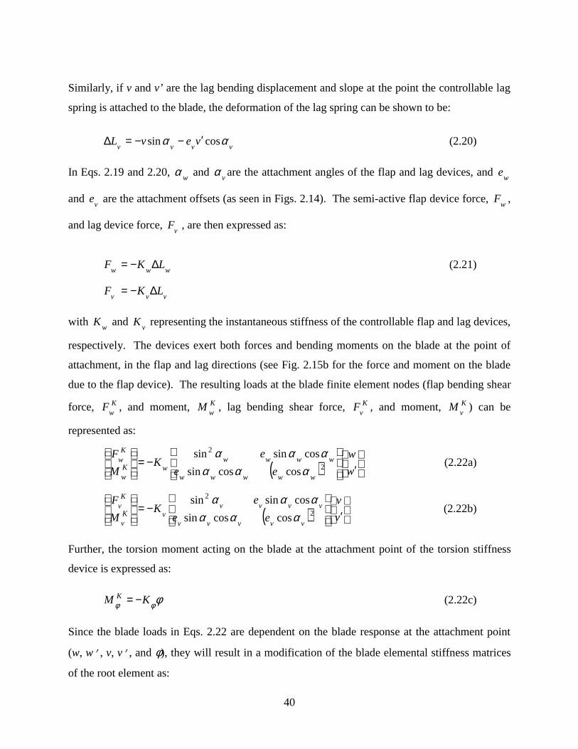
flap displacement, w, and slope, w’, at the attachment point is given by:

wwwwwewL αα cossin ′−−=∆ (2.19)

40

Similarly, if v and v’ are the lag bending displacement and slope at the point the controllable lag

spring is attached to the blade, the deformation of the lag spring can be shown to be:

vvvvvevL αα cossin ′−−=∆ (2.20)

In Eqs. 2.19 and 2.20, w

α and v

α are the attachment angles of the flap and lag devices, and w

e

and v

e are the attachment offsets (as seen in Figs. 2.14). The semi-active flap device force, w

F ,

and lag device force, v

F , are then expressed as:

wwwLKF ∆−= (2.21)

vvvLKF ∆−=

with w

K and v

K representing the instantaneous stiffness of the controllable flap and lag devices,

respectively. The devices exert both forces and bending moments on the blade at the point of

attachment, in the flap and lag directions (see Fig. 2.15b for the force and moment on the blade

due to the flap device). The resulting loads at the blade finite element nodes (flap bending shear

force, Kw

F , and moment, Kw

M , lag bending shear force, Kv

F , and moment, Kv

M ) can be

represented as:

( )

′

−=

w

w

ee

eK

M

F

wwwww

wwwwwK

w

Kw

2

2

coscossin

cossinsin

αααααα

(2.22a)

( )

′

−=

v

v

ee

eK

M

F

vvvvv

vvvvvK

v

Kv

2

2

coscossin

cossinsin

αααααα

(2.22b)

Further, the torsion moment acting on the blade at the attachment point of the torsion stiffness

device is expressed as:

φφφ KM K −= (2.22c)

Since the blade loads in Eqs. 2.22 are dependent on the blade response at the attachment point

(w, w’ , v, v’ , and φ), they will result in a modification of the blade elemental stiffness matrices

of the root element as:

41

[ ] [ ] [ ]DevicewwRootwwRootww

KKK )()( ψψ +=

[ ] [ ] [ ]DevicevvRootvvRootvv

KKK )()( ψψ += (2.23)

[ ] [ ] [ ]DeviceRootRoot

KKK )()( ψψ φφφφφφ +=

where [ ]Rootww

K , [ ]Rootvv

K , and [ ]Root

Kφφ are defined in Eq. B.2, and [ ]Deviceww

K )(ψ ,

[ ]Devicevv

K )(ψ , and [ ]Device

K )(ψφφ are defined in Eq. 2.24.

[ ]( )

////

////////

=

2

2

coscossin00

cossinsin00

0000

0000

)()(

wwwww

wwwwwDeviceww

ee

eKK

ααααααψψ (2.24a)

[ ]( )

////

////////

=

2

2

coscossin00

cossinsin00

0000

0000

)()(

vvvvv

vvvvvDevicevv

ee

eKK

ααααααψψ (2.24b)

[ ]

////////

=)(00

000

000

)(

ψψ

φ

φφK

KDevice

(2.24c)

The instantaneous stiffness of the discrete devices (Kw(ψ), Kv(ψ), and Kφ(ψ)) are defined earlier

in Eq. 2.15. With these modified elemental stiffness matrices, the blade equations are obtained

by assembling matrices from other beam elements. The modified blade equations can also be

represented by Eq. 2.14, and can be solved to yield blade response via the method presented in

Appendix E.

Comparing Eq. 2.24 to Eq. 2.18 suggests that the single spring model is representing the

controllable stiffness devices more accurately than the dual spring model. The single spring

model includes translation and rotational coupling effect (seen as off-diagonal terms in Eq. 2.24),

while the dual spring model does not account for the coupling effect.

42

2.3 Rotor blade damping variations

Due to limited availability of controllable stiffness devices and extensive work with controllable

dampers, it is natural to consider whether controllable dampers could be used in practice to

achieve helicopter vibration reduction, through cyclic variations of their properties. In addition,

all helicopters already employ passive lag dampers for aeromechanical stability augmentation,

and replacing them with semi-active controllable dampers may be relatively simple. The

controllable damper considered is a controllable orifice damper whose damping coefficient can

be modified by simply opening or closing an orifice valve. The following sections explain

damper modeling, incorporation of the controllable damper model, and blade root load

calculation.

2.3.1 Controllable orifice damper model

This section presents the development and verification of a mathematical model representing a

semi-active controllable orifice damper. A schematic sketch of the damper considered is shown

in Fig. 2.16. It comprises of a standard linear viscous damper augmented with a bypass, which

has a controllable valve. By varying the area of the controllable orifice through the application

of a voltage, the damper force or the equivalent damping coefficient can be controlled. The

change in damper characteristics with variation in orifice setting was experimentally

demonstrated in Ref. [107], and a fluid dynamics based model for the damper behavior was also

developed and validated in that study. The fluid dynamics based model involves computing the

instantaneous pressures developed in each chamber of the damper due to fluid flow through the

primary and bypass valves (see Fig. 2.16). The damper force can then be calculated from

pressure difference between the two chambers as follows:

)sgn()(21

uFAAPAPFfrppD

&+−−= (2.25)

where p

A is the piston area, r

A is the rod area, f

F is the static frictional force between the

piston and the damper casing, and u& is the piston velocity. Although Eq. 2.25 looks simple, the

fluid dynamics based model requires the solution of coupled differential equations governing the

43

pressures developed in each chamber. These equations (from Ref. [107]) are provided in

Appendix G for completeness. The controllable orifice area, con

A , as a function of applied

voltage, V , was reported to vary in the following manner:

[ ])exp(1)(max

ςγVAVAcon

−−= (2.26)

where max

A is the maximum orifice area, and γ and ζ are parameters obtained through

calibration of the valve. Varying the area of the controllable orifice changes the pressures

developed in the chambers (see Eqs. G.1 and G.2), and consequently, changes the damper

behavior. From Eq. 2.26 it is seen that for zero voltage the controllable orifice is completely shut

(con

A = 0), and for increasing values of voltage the orifice starts to open.

Figure 2.17 shows the force versus displacement damper hysteresis curves for various values of

orifice voltage (or orifice area). It is observed that the fluid dynamics model matches the

experimental data very well. Maximum damping is available for zero voltage when the bypass

valve is completely shut, and the available damping progressively reduces (hysteresis loop area

decreases) as the bypass valve opens with the application of a voltage. It is also seen that for a

specified orifice voltage, or orifice area, con

A , the hysteresis loop closely resembles that of a

linear viscous damper. Thus, in principle, an equivalent viscous damping coefficient,

2o

x

cycle) hysteresis under area Dissipated EnergyC

Ω=

π(

(2.27)

can be assigned to each hysteresis cycle, corresponding to a specified applied voltage. Figure

2.18 shows that the damper hysteresis cycle obtained using the full fluid dynamics based model

compares very well with that generated assuming a linear viscous damper with equivalent

damping coefficient from Eq. 2.27. This process can be repeated for different orifice voltages,

and a viscous damping coefficient determined for each case. A calibration curve of equivalent

damping coefficient as a function of bypass orifice voltage (or orifice area) can then be obtained,

as shown in Fig. 2.19. From the figure it is encouraging to note that – (i) the range of damping

variation available is very large, providing up to almost ±80% change from the mean damping

44

coefficient, and (ii) the calibration curve has a large linear range, which is beneficial from a

controller design standpoint.

Based on Fig. 2.19, the damping coefficient in the present study is assumed to vary linearly as:

)()(o

VVdV

dCCVC −+= or )()( VCCV

dV

dCCVC ∆+=∆+= (2.28)

which provides an accurate description of the damping behavior over a large range of variation

in input voltage. In Eq. 2.28, C is the nominal damping, o

V is the nominal voltage, and C∆ is

the variation in damping due to the voltage change V∆ . Such a reduced order controllable

damper model (Eq. 2.28) avoids the complexity of the full fluid dynamic based model, and can

be easily introduced in the rotor blade finite element equations.

However, before using the reduced order model in Eq. 2.28, additional verification is necessary.

In developing the reduced order model based on the calibration curve in Fig. 2.19, hysteresis

cycles for a series of different orifice settings were considered (Fig. 2.17); but the orifice area

(voltage) was never varied cyclically. In the present study, cyclic variations in the orifice voltage

are to be introduced at harmonics of the rotor frequency. It is necessary to verify that the

reduced order model is valid (produces damper force predictions, or hysteresis cycles, very

similar to those obtained using the full fluid dynamics based model) even when the orifice is

controlled cyclically, at harmonics of the damper motion frequency.

Figures 2.20a and 2.20b, respectively, show the hysteresis cycles predicted when cyclic variation

in the orifice voltage is introduced at the damper motion frequency and at twice the motion

frequency. In both figures, the results from the reduced order model (Eq. 2.28) are practically

identical to those from the full fluid dynamics model (Eqs. G.1, G.2 and 2.25), thus establishing

the validity of the reduced order model, even for cyclically varying orifice voltages. It should be

noted that a cyclic variation in orifice voltage, of amplitude V∆ about a mean voltage of o

V ,

produces a change in the shape of the hysteresis cycle but no change in the area enclosed (which

remains the same as that when a constant voltage o

V is applied) – cycles in Figs. 2.18, 2.20a, and

45

2.20b all have the same enclosed area. This suggests that while cyclic variation in voltage will

produce higher harmonic forces that could be exploited to reduce hub vibrations, it is unlikely to

compromise the energy dissipation characteristics of the damper (which are determined only by

the mean orifice voltage, o

V , or, in effect, the mean damping coefficient, C ). In addition, a

change in the phase of the cyclic voltage input would result in the hysteresis curves shown in

Figs. 2.20 undergoing a corresponding rotation, but again, the area enclosed is unchanged.

In the present study controllable orifice dampers are introduced in the rotor blade root region,

and the voltage varied cyclically with time, or with azimuthal position, ψ (since the system is

periodic). Thus the reduced order model in Eq. 2.28 can be represented in the following form

)()( ψψ CCC ∆+= (2.29)

where the variation in damping, C∆ , about the mean value, C , is expressed in terms of the

independent variable, ψ , rather than the dependent variable, )(ψV .

2.3.2 Inclusion of controllable dampers into blade equations

Controllable dampers are introduced in the blade root region in the flap and lag directions (see

schematic in Fig. 2.21) to produce semi-active forces that modify the blade response and reduce

hub vibrations. Flap and lag controllable dampers are introduced because preliminary studies

(presented later in Chapters 6 and 7) showed that semi-active stiffness variations particularly

with the flap and lag devices are effective in reducing hub vibrations. Using the reduced order

damper model (Eq. 2.29), cyclic variations in the flap and lag damping coefficients are

represented, without loss of generality, in the following form:

[ ]∑=

+∆+=∆+=N

n

wn

nwwwww

nCCCCC1

)sin()()( φψψψ (2.30)

[ ]∑=

+∆+=∆+=N

n

vn

nvvvvv

nCCCCC1

)sin()()( φψψψ

Again, “n” represents the frequency of the cyclic damping variations and “φn” represents the

phase angle corresponding to damping variation at n/rev. The amplitudes of flap and lag

46

damping variations, w

C∆ and v

C∆ are expressed as percentages of their baseline values ( wC

and vC , respectively). It should be noted that from a practical standpoint there is a limit to the

maximum variations in damping coefficient achievable with the controllable orifice dampers,

and this was taken to be ± 80% of the baseline damping coefficients ( wC , or vC ), based on Fig.

2.19. Equations 2.30 can be written in a compact form as:

[ ]∑=

+∆+=∆+=N

nn

nDDDDD

nCCCCC1

)sin()()( φψψψ (2.31)

The damper configuration and attachment geometries are similar to that shown in Fig. 2.14,

except that the controllable stiffness devices are replaced with controllable dampers. Again, the

flap and lag dampers are attached to the rotor blade at a finite element node so that the semi-

active forces and moments exerted on the blade are easily accounted for, since blade velocity at

the node is readily available. The semi-active damper force generated depends on the

instantaneous damping coefficient of the controllable dampers as well as the blade flap and lag

velocities at the attachment point, which determines the piston velocities of the controllable

dampers. Figure 2.22a shows the change in the flap damper length due to flap bending

deformations of the blade. From the geometry and kinematics it can be shown that the flap

damper deformation due to flap displacement, w, and slope, w’, at the attachment point is given

by Eq. 2.19, and the piston velocity of the flap damper can be written as:

wwwwwewL αα cossin &&& ′−−=∆ (2.32a)

Similarly, if v and v’ are the lag bending displacement and slope at the point of attachment of the

lag damper to the blade, the piston velocity of the lag damper can be shown to be:

vvvvvevL αα cossin &&& ′−−=∆ (2.32b)

Again, w

α and v

α are the attachment angles of the flap and lag dampers, and w

e and v

e are the

attachment offsets (as seen in Figs. 2.14). The semi-active flap damper force, w

F , and lag

damper force, v

F , are then expressed as:

47

wwwLCF &∆−= (2.33)

vvvLCF &∆−=

with w

C and v

C representing the instantaneous damping coefficients of the controllable flap and

lag dampers, respectively. The dampers exert forces and bending moments on the blade at the

point of attachment in both the flap and lag directions (see Fig. 2.22b for the force and moment

due to the flap damper). The resulting loads at the blade finite element nodes (flap bending

shear, Dw

F , and moment, Dw

M , and lag bending shear, Dv

F , and moment, Dv

M ) can be expressed

as:

( )

′

−=

w

w

ee

eC

M

F

wwwww

wwwwwD

w

Dw

&

&2

2

coscossin

cossinsin

αααααα

(2.34)

( )

′

−=

v

v

ee

eC

M

F

vvvvv

vvvvvD

v

Dv

&

&2

2

coscossin

cossinsin

αααααα

Since the blade loads contain velocity-dependent terms, they will result in a modification of the

blade elemental damping matrices of the root element as follows.

[ ] [ ] [ ]DamperwwRootwwRootww

CCC )()( ψψ += (2.35)

[ ] [ ] [ ]DampervvRootvvRootvv

CCC )()( ψψ +=

where [ ]Rootww

C and [ ]Rootvv

C are defined in Eq. B.3, and [ ]Damperww

C )(ψ and [ ]Dampervv

C )(ψ are

defined in Eq. 2.36.

[ ]( )

////

////////

=

2

2

coscossin00

cossinsin00

0000

0000

)()(

wwwww

wwwwwDamperww

ee

eCC

ααααααψψ (2.36a)

[ ]( )

////

////////

=

2

2

coscossin00

cossinsin00

0000

0000

)()(

vvvvv

vvvvvDampervv

ee

eCC

ααααααψψ (2.36b)

48

The instantaneous damping coefficient of the flap and lag dampers, Cw(ψ) and Cv(ψ), are given

in Eq. 2.30. Then the modified blade equations are obtained by assembling all the other matrices

with the modified elemental damping matrix. The modified blade equations can be represented

by Eq. 2.37.

AFFKqqCCqM +=+∆++ &&& )(ψ (2.37)

where )(ψC∆ represents the component of the damping matrix with periodically varying terms

due to the controllable orifice dampers. The blade responses are obtained by solving these blade

equations using the method described in Appendix E.

2.3.3 Blade root loads and hub loads calculation

It should be noted that introduction of the controllable flap and lag dampers, as shown in Figs.

2.21, creates multiple paths for transfer of loads to the rotor hub. Blade root loads calculation

outlined in Section 2.1.4 can still be used, but the semi-active forces generated by the

controllable dampers have to be considered. The shear forces and moments at the root of the

flexbeam are denoted with the superscript “flex”. In addition, the superscript “damper” is used

to denote the shear forces and moments appearing at the root of the damper. See Figures 2.23a

and 2.23b, respectively, for the root vertical shear and the drag shear forces due to the flexbeam

and the damper. The “total” blade root shear forces (z

S and x

S in Figs. 2.23a and 2.23b), then,

are summations of the flexbeam and damper contributions (z

S = flexz

S + damperz

S and x

S = flexx

S

+ damperx

S ). It is these “total” shear forces that are considered when calculating the vibratory hub

forces. Thus, the vertical shear force, flexz

S , and the drag shear force, flexx

S , at the root of the

flexbeam can be expressed as,

ww

nodes of

k

kz

flexz

FfS αsin#

1

−= ∑=

(2.38)

vv

nodes of

k

kx

flexx

FfS αsin#

1

−= ∑=

49

The vertical shear force, damperz

S , and the drag shear force, damperx

S , at the root of the flap and lag

dampers are simply

wwdamperz

FS αsin= (2.39)

vvdamperx

FS αsin=

Thus, from Eqs. 2.38 and 2.39, the total blade root shear forces (z

S and x

S ) are obtained as,

zS = flex

zS + damper

zS = ∑

=

nodes of

k

kz

f#

1

(2.40)

xS = flex

xS + damper

xS = ∑

=

nodes of

k

kx

f#

1

It is interesting to note that the total blade root shears (Sz and Sx) used in the calculation of the

hub forces have only aerodynamic and inertial contributions (contained in the kz

f ’s and kx

f ’s),

and the damper loads cancel out (see Eq. 2.40). These equations for blade root shears are the

same as the equations presented in Eq. 2.10a. In a similar manner it could be shown that any

direct damper contributions to the root radial shear force, and the blade root moments, cancel out

as well. The damper, however, has modified the blade response, and the inertial and

aerodynamic loads (which are dependent on the blade response). Further, the loads at the

flexbeam root are modified due to the presence of the controllable damper (see Eq. 2.38). After

blade root loads are obtained, hub loads can be calculated using the method in Section 2.1.4.

2.4 Influence of semi-active stiffness and damping variation

From previous sections, it is seen that the blade equations are modified when semi-active

stiffness or damping variations are introduced as presented in Eq. 2.14 and 2.37, respectively.

qKFFqKqCqM A )(ψ∆−+=++ &&& (2.14a)

qCFFKqqCqM A &&&& )(ψ∆−+=++ (2.37a)

where )(ψK∆ represents the stiffness variations and )(ψC∆ represents the damping variations.

Clearly, the qK )(ψ∆ (due to cyclic stiffness variations) and qC &)(ψ∆ (due to cyclic damping

variations) terms can be regarded as unsteady semi-active loads that can be used to modify the

50

blade response as desired. Traditionally for a 4-bladed rotor helicopter, HHC or IBC uses higher

harmonic pitch input at 3/rev, 4/rev, and 5/rev to produce higher harmonic unsteady aerodynamic

forces of those frequencies, and change blade response and reduce vibration. With the present

semi-active approach, even lower harmonic variations in stiffness, )(ψK∆ , or damping, )(ψC∆ ,

at 2/rev and 3/rev, are able to generate the desired higher harmonic semi-active loads, qK )(ψ∆

or qC &)(ψ∆ , at 3/rev, 4/rev, and 5/rev, for vibration reduction, since the blade response and

velocity, q and q& , themselves already contain harmonics of rotor frequency (1/rev, 2/rev, 3/rev,

etc.). This will be demonstrated in the result sections that 2/rev and 3/rev stiffness or damping

variations are particularly effective in reducing 4/rev hub vibrations.

Calculation of blade root loads and hub loads are unchanged with the introduction of stiffness

and damping variations, since all direct contributions of the semi-active loads (from the stiffness

and damping variations) to blade root loads are canceled out. In other words, influence of the

stiffness and damping variations has to be taken into account in the calculation of the blade

response, but its effect on the blade root loads is only to the extent that the changed response of

the blade affects the aerodynamic and inertial loading. This suggests that the stiffness and

damping variations generate semi-active loads that change blade response, and indirectly

influence the blade root loads, which in turn can be used to reduce the hub vibrations.

51

C.G.

Y fF

y

D f

Fx

T tr

Xht

X tr

Mz

Mz f

TOP VIEW

LEFT-SIDE VIEW

h

F z

F xM y

M y f

W

X cg

D fL h t

Z tr

α s

h

Fy

Fz

M x

Ttr

M xf

W

Ycg

φV

Zht

REAR VIEW

Figure 2.1: Forces and moments exert on a helicopter in a level forward flight

Z

Y

Z

X

Y

X

52

w1

w2

v2

v11

2v’2

v’1φ1

φ 2

φ3

w’1

w’

Figure 2.2: Spatial discretization of a rotor blade using Finite Element Method

M1

M2

M3

M4

M5

Figure 2.3: Global mass matrix of a rotor blade with 5 spatial elements

ψ

ψ = 0

Figure 2.4: Discretization of azimuthal position for blade response calculation using FiniteElement in time method

53

Figure 2.5: Flowchart of coupled rotor/trim response calculation procedure

Update control settings

and orientations

START TRIM

Initial guess values

(control settings and orientations)

Solve blade response

Compute hub loads

Calculate vehicle equilibrium

No

END TRIM

Yes

Satisfy equilibrium

54

fz1

fz2

fz3

fz4

fz5

fz6

fx3

fx1

fx2

fx4

fx5

fx6

l1

l2

l3

l5l4

Figure 2.6: Nodal blade shear forces in vertical and chordwise directions

mβ1

mβ2

mβ3

mβ4

mβ5

mβ6

Figure 2.7: Nodal blade moments in flapwise direction

Ω

SrSx

x

y

ψ

Mβ Mφ

z

Mζ

Sz

Figure 2.8: Blade root shear forces and moments

55

Ω

SrSx

x

y

ψ

Mβ Mφ

z

Mζ

Sz

Mx

My

Fy

Fx

Fz Mz

Figure 2.9: Transformation between Hub loads and Blade Root Loads

Root Element(stiffness varying cyclically)

Figure 2.10: Stiffness variation of the root element

Figure 2.11: Schematic sketch of discrete controllable stiffness devices

Controllable LagStiffness Device

Controllable FlapStiffness Device

Controllable TorsionStiffness Device

56

Figure 2.12: Mathematical idealization of discrete controllable stiffness devices using dual springmodel in (a) flap and (b) lead-lag directions.

Figure 2.13: Mathematical idealization of discrete controllable stiffness devices using singlespring model in (a) flap, (b) lead-lag, and (c) torsional directions.

(b)

(a)

(a)

(c)

(b)

Kw

Kφ

Kv

Kv

Kv’

Kw’

57

Figure 2.14: Configuration and attachment geometry of controllable stiffness devices,

(a) flap device and (b) lag device

Figure 2.15: (a) Deformation of the flap device due to blade bending, and(b) Loads exerted on the blade at attachment point by the flap device

ew

αw

Kw

αv

ev

Kv

(a) (b)

(a) (b)Fw

Mw

Lw-∆Lw

Lw

Fw = - Kw ∆Lw

w

w′

K

K

58

Figure 2.16: Schematic of a semi-active controllable damper

(a) (b)

Figure 2.17: Force/Displacement hysteresis loops for different bypass orifice settings (valvevoltages); (a) experiment, (b) fluid dynamic model simulations (from Ref. 103)

-2000

-1500

-1000

-500

0

500

1000

1500

2000

-30 -20 -10 0 10 20 30

Fluid Dynamics Model

Equivalent Damping Coefficient

Figure 2.18: Force/Displacement hysteresis cycles produced by the fluid dynamics based dampermodel and an equivalent damping coefficient model (at a specified orifice command voltage Vo)

Bypass with ControllableOrifice

Primary OrificeAccumulator

Chamber 2 Chamber 1

u

Rod

Pist

on

Increasing Voltage(or orifice area)

Displacement (mm)

Dam

per

For

ce (

N)

59

0

5

10

15

20

0 1 2 3

= 0.5Hz

= 1Hz

= 1.5Hz

= 2Hz

Figure 2.19: Calibration curve for equivalent viscous damping coefficient as a function of orificevoltage

-2500

-2000

-1500

-1000

-500

0

500

1000

1500

2000

-30 -20 -10 0 10 20 30

Fluid Dynamic Model

Reduced Order Model

-2000

-1500

-1000

-500

0

500

1000

1500

2000

-30 -20 -10 0 10 20 30

Fluid Dynamic Model

Reduced Order Model

(a) (b)Figure 2.20: Damper hysteresis loops for prescribed damper motion at frequency Ω and

cyclically varying orifice voltage (a) V=Vo+∆Vsin(Ωt) and (b) V=Vo+∆Vsin(2Ωt)

Figure 2.21: Schematic of rotor blade with controllable flap and lag dampers

Bypass Orifice Command Voltage (V)

Dam

ping

Coe

ff. C

(N

.s/m

m)

Increasingfrequency

Vo

C

Slope = dVdC

C = C +dVdC

(V-Vo)

ΩΩ

ΩΩ

Displacement

Dam

per

For

ce (

N)

Displacement

Controllable Flap Damper

Controllable Lag Damper

60

Figure 2.22: (a) Deformation of the flap damper due to blade bending, and (b) loads exerted onthe blade at attachment point by the flap damper

Figure 2.23a: Blade root vertical shear, Sz, with contributions from the flexbeam, Szflex (obtained

by summing vertical shear forces, fzi, along blade Finite Element DOF’s), and the flap damper,

Szdamper

Figure 2.23b: Blade root drag shear, Sx, with contributions from the flexbeam, Sxflex (obtained by

summing drag shear forces, fxi, along blade Finite Element DOF’s), and the lag damper, Sx

damper

(a) (b) Dw

F

Dw

M

L-∆Lw

LFw = - Cw ∆Lw

w

w′

αw

sin αw

Szflex Fw

Fw

Szdamper

Sz = +Szflex

Szdamper

fz1

fz2

fz3

fz4

sin αvFv

αv

Fv

Sxflex

Sxdamper

Sx = +Sxflex

Sxdamper

fx1

fx2

fx3

fx4

61

Chapter 3

Optimal Semi-Active Control Scheme

3.1 Calculation of optimal semi-active inputs

A frequency-domain approach is considered in determining optimal semi-active input, ∆U,

(which can represent either stiffness variation, )(ψK∆ , or damping variation, )(ψC∆ ). This

frequency domain method is similar to that developed in Ref. 117 and widely employed in

previous active vibration reduction studies. The semi-active input, ∆U, is expressed in

frequency-domain and comprises of amplitudes of sine and cosine components of stiffness or

damping variations (at harmonics of rotational speed). Examples of the semi-active inputs are

shown in Eq. 3.1a and 3.1b for stiffness and damping variations, respectively.

T

device lag the ofiations tiffnesss rev

sv

cv

sv

cv

device flap the ofiations tiffnesss rev

sw

cw

sw

cw

KKKK KKKKU ][

var/3,2

3322

var/3,2

3322

44444 344444 2144444 344444 21∆∆∆∆∆∆∆∆=∆ (3.1a)

T

damper lag the ofiations ampingd rev

sv

cv

sv

cv

damper flap the ofiations ampingd rev

sw

cw

sw

cw

CCCC CCCCU ][

var/3,2

3322

var/3,2

3322

44444 344444 2144444 344444 21∆∆∆∆∆∆∆∆=∆ (3.1b)

where superscript “nc” represents the cosine component at n/rev and superscript “ns” represents

sine component at n/rev. The rotor hub vibration is expressed in frequency domain as, z, which

consists of sine and cosine components of all vibratory hub loads, and is defined in Eq. 3.2.

[ ] Ts

zc

zs

yc

ys

xc

xs

zc

zs

yc

ys

xc

xMMMMMMFFFFFFz 444444444444= (3.2)

where superscripts “4c”and “4s” denote cosine and sine components of the 4/rev vibratory hub

loads, respectively. It is assumed that the semi-active input, ∆U, and hub vibration, z, are related

through a transfer matrix, T, as follows:

62

z = zo + T ∆U (3.3)

where “zo” is the baseline 4/rev hub vibration (without any semi-active input). The transfer

matrix, T, is numerically calculated by perturbation of individual semi-active input components,

about the baseline configuration.

The control algorithm, adapted from Ref. 117, is based on the minimization of a composite

quadratic objective function, J, defined as:

J = Jz + Ju = 321

zJ

zT zWz +

43421uJ

uT UWU ∆∆ (3.4)

where “Wz” represents the weighting on hub vibration ( 1

6

100 −= T

oozzzW ), and “Wu”

represents the penalty weighting on semi-active input (Wu is usually set to an identity matrix,

unless otherwise stated). In the result Chapters, Jz = zT Wz z (which is a measure of the vibration

level) is used as a performance index; with smaller values of Jz indicating more vibration

reduction due to semi-active inputs. The semi-active input index, Ju, can represent the amount of

semi-active input required for vibration reduction. The optimal semi-active input (stiffness or

damping variations) can be determined using both gradient and non-gradient based methods.

3.1.1 Gradient-based optimization

The optimal semi-active input can be obtained using a gradient-based optimization approach. An

optimal input is obtained by substituting Eq. 3.3 into Eq. 3.4 and setting the derivative of the

objective function with respect to semi-active inputs to zero (∂J/∂∆U = 0). The resulting optimal

semi-active input is presented in Eq. 3.5.

∆U = -(TTWzT + Wu )-1TTWz zo (3.5)

Equation 3.5 suggests that the calculation of semi-active input requires prior knowledge of the

baseline hub vibration, zo (measured or calculated), and transfer matrix, T. This semi-active

control scheme is equivalent to an open-loop scheme, which might produce non-optimal inputs

when there is a change in operating condition or rotor configuration. If the change occurs, the

63

semi-active input would have to be re-evaluated since the baseline hub vibration and/or transfer

matrix may change.

3.1.2 Non-Gradient-based optimization

The optimal semi-active input can also be determined using a non-gradient-based optimization

method. The optimization method considered is based on Genetic Algorithm (GA) approach

[118]. An optimal input is determined through an evolutionary process replicating natural

selection. Any possible semi-active input, ∆U, is coded into a binary string called an individual.

Initially, several individuals are generated randomly to make up the first generation. For every

individual in the generation, a “fitness function” is evaluated based on the same objective

function defined in Eq. 3.4. The “most fit” individuals in that generation, or the ones that

produce the minimum objective function, will be chosen to produce individuals in the next

generation through a mating and mutation process. After repeating this process for several

generations, the procedure will produce the individual with the highest fitness, which can be

decoded back to yield optimal semi-active input that minimizes the objective function. For the

genetic algorithm simulations conducted in the present study, the number of individuals in each

generation is 20, and the number of generations is 50-200. In general, the amount of time

involved in calculating an optimal input using this GA approach is a lot longer than that used by

the gradient based approach.

64

Chapter 4

Sensitivity Study

This Chapter presents preliminary vibration reduction results using root element stiffness

variations, described in Section 2.2.1. The effectiveness of root element stiffness variations on

reducing hub vibration is examined at a nominal advance ratio of 0.3, using Drees inflow model.

The helicopter considered is a 4-bladed hingeless rotor helicopter whose rotor-fuselage

properties are given in Appendix H (Table H.1). Stiffnesses of the root elements of the blades

are varied cyclically to produce hub vibration reduction (see Eq. 2.12 and Fig. 2.10). Five beam

elements are used to model the rotor blade, and 6 modes (2 flap, 2 lag, and 2 torsion modes) are

used in modal transformation. The baseline hub vibrations and blade root loads, without any

root element stiffness variations, are given in Table 4.1a and Table 4.1b, respectively. Section

4.1 shows sensitivity of vibratory hub loads to root element flap, lag, and torsion stiffness

variations at various frequencies, amplitudes, and phases. Underlying mechanism of hub

vibration reduction is presented in Section 4.2. Influence of the root element stiffness variations

on blade root loads is shown in Section 4.3. Further, Section 4.4 illustrates effectiveness of the

root stiffness variation in reducing hub vibration at different advance ratios. A brief summary of

the results in this chapter is presented in Section 4.5.

4.1 Influence of root element stiffness variations on vibratory hub loads

The Influence of individual variations in root element flap, lag, and torsion stiffness on hub

vibration is examined. The influence of different harmonics (1/rev, 2/rev, 3/rev, 4/rev, and

5/rev) of the stiffness variations is also considered. For each harmonic of the stiffness variations,

the associated phase angle (see Eq. 2.12) is varied to demonstrate sensitivity of vibratory hub

loads to the stiffness variation.

4.1.1 Cyclic variation in flap stiffness

The effects of cyclic variations in flapwise stiffness of the root element (flap stiffness) are

examined in this section. For a 1/rev variation in flap stiffness, Figs. 4.1a and 4.1b show the

65

vibratory hub forces and moments, respectively, as a function of phase angle, φ, of the flap

stiffness variation. The amplitude of the stiffness variation considered is 15% of the baseline flap

stiffness (∆EIβ1p = 0.15 βEI ). The vibratory forces and moments are non-dimensionalized by

their respective baseline values (denoted as 100%). From Fig. 4.1a it can be seen that while the

hub in-plane shear forces, Fx4p and Fy

4p, are virtually insensitive to 1/rev flap stiffness variations,

the hub vertical shear force, Fz4p, can be reduced by roughly 20% at an “optimal” phase angle of

about 225o. Figure 4.1b indicates that the hub moments are mildly sensitive to 1/rev flap

stiffness variations. At the phase angle, φ = 225o, small reductions in hub moments (of no more

than 10%) can be obtained in addition to the reduction in Fz4p.

Figure 4.2 shows the influence of 2/rev variations in flap stiffness on the vibratory hub loads.

The amplitude of the variation, ∆EIβ2p, is 15% of the baseline flap stiffness, βEI . It is seen from

Fig. 4.2a that at an “optimal” phase angle of around 240o, a 70% reduction in hub vertical shear

force, Fz4p, can be achieved. The hub in-plane shears, Fx

4p and Fy4p, show very little sensitivity to

a 2/rev variation in flap stiffness. Figure 4.2b indicates that the hub moments are moderately

sensitive to 2/rev flap stiffness variations, with a 15-20% increase in the hub in-plane moments,

Mx4p and My

4p, observed at φ = 240o.

Figure 4.3 shows the influence of 3/rev variations in flap stiffness on the vibratory hub loads.

The amplitude of the variation, ∆EIβ3p, is 15% of the baseline flap stiffness, βEI . All vibratory

hub forces and moments show large sensitivity to 3/rev variations in flap stiffness. Figure 4.3a

indicates that a substantial 70% reduction in the hub in-plane shear forces, Fx4p and Fy

4p, and a

40% reduction in the hub vertical shear, Fz4p, can be achieved at a phase angle of around 0o. At

this phase angle, the hub torque, Mz4p, is unchanged and the pitching moment, My

4p, is decreased

by 15%, but the rolling moment, Mx4p, is increased by 20% (Fig. 4.3b). Alternatively, if a phase

angle of around 45o is selected, 60% and 85% reductions in hub in-plane moments, Mx4p and My

4p,

and an approximately 30% reduction in all hub forces can be achieved. This phase angle,

though, produces a 25% increase in the vibratory hub torque, Mz4p.

66

A 4/rev flap stiffness variation with an amplitude as low as 5% of the baseline flap stiffness

(∆EIβ4p = 0.05 βEI ) produced a more than 200% increase in vibratory hub vertical shear, Fz

4p,

over the entire range of phase angles. The system appears to be “overdriven” with the stiffness

variations actually producing significant vibrations rather than merely canceling the original

vibrations. Conceivably, the amplitude of stiffness variation could be further reduced, but

smaller amplitudes would require high precision in stiffness variation. A 5/rev flap stiffness

variation had the greatest influence on the in-plane vibratory hub moments. For an amplitude of

variation of 5% of the baseline flap stiffness (∆EIβ5p = 0.05 βEI ), up to 60% reductions in the in-

plane hub moments were possible. However, the phase angles that produced a decrease in the

rolling moment, Mx4p, increased the pitching moment, My

4p, by a comparable amount, and vice-

versa. Thus, 4/rev and 5/rev variations in flap stiffness are not considered as candidates for

reduction of vibratory hub loads.

4.1.2 Cyclic variation in lag stiffness

The effects of cyclic variations in chordwise stiffness of the root element (lag stiffness) are

examined in this section. A 1/rev variation in lag stiffness, of amplitude 15% of the baseline lag

stiffness (∆EIζ1p = 0.15 ζEI ), was first considered. The vibratory hub forces and moments were

found to be relatively insensitive to 1/rev lag stiffness variations, with reductions in vibratory

hub loads of no more than 5-7%, relative to the baseline values.

The influence of 2/rev lag stiffness variations on the vibratory hub loads is shown in Fig. 4.4.

The amplitude of variation, ∆EIζ2p, is 15% of the baseline lag stiffness, ζEI . The vibratory in-

plane hub forces and the hub torque are most sensitive to the 2/rev lag stiffness variations. From

Fig. 4.4a it is seen that at an “optimal” phase angle of about 90o, the in-plane shear forces, Fx4p

and Fy4p, are reduced by about 20% and 30%, respectively. At the same phase angle, the hub

torque, Mz4p, is simultaneously reduced by about 20%.

Figure 4.5 shows the influence of 3/rev variations in lag stiffness on the vibratory hub loads.

The amplitude of the variation, ∆EIζ3p, is 5% of the baseline lag stiffness, ζEI . In Fig. 4.5a it is

seen that at a phase angle of 225o, the hub vertical shear, Fz4p, can be reduced by 40% without

67

adversely affecting any of the other hub forces or moments. Alternatively, Fig. 4.5b indicates

that a phase angle of 135o produces an 85% reduction in hub torque, Mz4p, without adversely

affecting any other hub forces or moments. Any phase angle between 135o and 225o produces

simultaneous reductions in Fz4p and Mz

4p. The in-plane hub forces and moments are relatively

insensitive to 3/rev lag stiffness variations. At a phase of 135o, if larger amplitudes of stiffness

variation are considered, the vibratory hub torque starts to increase since the system is

“overdriven” and the stiffness variations are producing the vibrations rather than merely

cancelling them. Figure 4.6a clearly illustrates this principle. It is seen in the figure that as

∆EIζ3p increases from 0.02 ζEI to 0.05 ζEI , larger reductions in Mz

4p can be achieved. However,

an increase in ∆EIζ3p to 0.10 ζEI produces smaller reductions in Mz

4p, and for ∆EIζ3p =0.15 ζEI ,

the vibrations actually increase, at any phase angle. Figure 4.6b shows the maximum reduction

in Mz4p versus magnitude of stiffness variation (at the optimal phase angle) for 2/rev as well as

3/rev lag stiffness variations. It is seen from the figure that for 2/rev variations, more vibration

reduction is achieved as ∆EIζ increases. However, the hub vibrations are more sensitive to 3/rev

lag stiffness variations, so small amplitudes are able to produce large reductions. If the

amplitude is further increased, the system is “overdriven” and the stiffness variations produce the

vibrations.

A 4/rev lag stiffness variation (of amplitude ∆EIζ4p = 0.05 ζEI ) produced about 40% variations in

all the vibratory hub forces and the hub torque. However, the phase angles that produced a

decrease in the vibratory hub drag, Fx4p, produced a corresponding increase in the side-force, Fy

4p,

and vice-versa. Thus, 4/rev variations in lag stiffness are not considered as a candidate for

reduction of vibratory hub loads.

Figure 4.7 shows the influence of 5/rev variations in lag stiffness on the vibratory hub loads.

The amplitude of the variation, ∆EIζ5p, is 5% of the baseline lag stiffness, ζEI . From Fig. 4.7b it

is seen that the hub torque, Mz4p, is virtually eliminated at a phase of about 180o, but components

of hub forces are simultaneously increased by 10-20% (Fig. 4.7a). However, a phase angle of

about 200o can reduce the hub torque, Mz4p, by over 85% without adversely affecting the hub

forces. The in-plane moments, Mx4p and My

4p, are insensitive to 5/rev lag stiffness variations.

68

4.1.3 Cyclic variation in torsion stiffness

The effects of cyclic variations in torsional stiffness of the root element are examined in this

section. 1/rev and 2/rev variations in torsion stiffness, of amplitude 15% of the baseline torsion

stiffness, were found to have relatively little influence on the vibratory hub forces and moments

(with hub vibration reductions of no more than 5-7% of the baseline values). Hence 1/rev and

2/rev variations in torsion stiffness are not considered for reduction of vibratory hub loads.

The effect of 3/rev torsion stiffness variation on the vibratory hub loads is shown in Fig. 4.8.

The amplitude of variation, ∆GJ3p, is 15% of the baseline torsion stiffness, GJ . Figure 4.8a

indicates that while the vibratory in-plane hub forces are insensitive to 3/rev torsion stiffness

variations, a 15% reduction in hub vertical shear, Fz4p, can be achieved if a phase angle of 315o -

360o is selected. For these values of phase angle, the vibratory hub moments show no significant

change (Fig. 4.8b).

Figure 4.9 shows the influence of 4/rev variations in torsion stiffness on the vibratory hub loads.

The amplitude of variation, ∆GJ4p, is again 15% of the baseline torsion stiffness, GJ . Figure

4.9a indicates that while the in-plane vibrations, Fx4p and Fy

4p, are insensitive to the stiffness

variations, a 20% reduction in vertical shear, Fz4p, can be achieved for an “optimal” phase angle

of around 90o - 135o. The influence of 4/rev torsion stiffness variations on vibratory hub

moments is fairly insignificant (Fig 4.9b).

5/rev variations in torsion stiffness (with ∆GJ5p = 0.15GJ ) were able to produce reductions in

Fz4p of no more than 8%. Other vibratory hub loads showed even lower sensitivity. Hence 5/rev

torsion stiffness variations are not considered for reduction of hub vibrations.

4.1.4 Summary of beneficial root element stiffness variations

Harmonic variations in flap, lag, and torsion stiffness of the root element that produced

significant reductions in vibratory hub loads are summarized in Table 4.2. Listed in the table are

the amplitudes of stiffness variation required (as a percentage of the baseline stiffness), the

“optimal” phase, and the corresponding changes in the components of vibratory hub loads. A

69

1/rev flap stiffness variation is not considered, since significantly larger reductions in the hub

vertical force, Fz4p, can be achieved using 2/rev variations in flap stiffness. Although torsion

stiffness variations produce reductions in Fz4p that are comparable to those achieved using a 1/rev

flap stiffness variation, these are retained to assess comparison between the flap stiffness versus

torsion stiffness variations. In general, it can be observed from Table 4.2 that torsion stiffness

variations produce only moderate reductions in Fz4p. Lag stiffness variations can produce

reductions in all hub forces and the hub torque. Flap stiffness variations are probably the most

versatile, and have the potential to reduce all hub forces and the in-plane hub moments.

4.2 Mechanism for reduction of vibratory hub loads

In the previous section, stiffness variations that produced reductions in vibratory hub loads were

identified (Table 4.2). For these stiffness variations, the present section examines the mechanism

by which the vibration reduction is achieved. Specifically, since inertial and aerodynamic

components of the various blade root loads contribute significantly to the hub loads, this section

seeks to understand the individual change or the combination of changes, in these components

that leads to the reduction of the vibratory hub loads.

The following comments can be made about all the reductions in vibratory hub moments. The

hub roll and pitch moments, Mx4p and My

4p, have contributions from the blade root flapping

moment, Mβ, and the blade root pitching moment, Mφ. However, for the symmetric airfoil

considered in the present study, the root pitching moments in the absence of stall are

considerably smaller than the blade root flapping moment. Further, the blade root flapping

moment contribution to Mx4p and My

4p is dominated by the inertial component and it is reductions

in the inertial component of Mβ (due to stiffness variations) that produce reductions in Mx4p and

My4p. The blade root lag moment contributes to the vibratory hub yaw moment, Mz

4p. The blade

root lag moment is also dominated by the inertial contribution, and reduction in Mz4p is achieved

when stiffness variation reduces this component. The mechanisms for reduction of the vibratory

hub forces are more varied, and are discussed below.

70

For the 2/rev flap stiffness variation, Fig. 4.10 depicts, vectorially, the inertial and aerodynamic

components of Fz4p. Compared to the baseline rotor (no stiffness variations) the aerodynamic

component increases slightly. The inertial component decreases somewhat in magnitude (by no

more than 20%) but undergoes a phase change. This phase change in the inertial component

results in a significantly reduced vectorial sum (of the inertial and aerodynamic components), so

that there is a 70% net reduction in the total Fz4p load.

For the 3/rev flap stiffness variation, a phase angle of 45o produced 30% reductions in vibratory

hub forces, and 60% and 85% reductions, respectively, in the hub roll and pitch moments, Mx4p

and My4p. The blade root radial shear force, Sr, and drag shear force, Sx, contribute to the in-plane

hub forces. Figure 4.11 shows the contributions of Sr and Sx to Fx4p, vectorially. It clearly

indicates that although the individual contributions of Sr and Sx to Fx4p have not changed in

magnitude, an increase in the relative phase angle results in a smaller net Fx4p. The reduction in

Fy4p occurs in a similar manner. Figure 4.12 depicts, vectorially, the inertial and aerodynamic

components of Fz4p. Compared to the baseline rotor, the aerodynamic component decreases

slightly and the inertial component decreases to a larger extent (by about 40%). While both

components individually undergo a change in phase, there is little change in the relative phase

angle. Thus it can be concluded that the 30% reduction in the total Fz4p load is due to the

decrease in the magnitude of the contributing aerodynamic and inertial components.

The 2/rev lag stiffness variation produced 20%-30% reductions in the hub in-plane forces, which

was due to decreases in both the blade root radial shear and drag shear contributions to Fx4p and

Fy4p. These decreases, specifically, occurred due to reductions in the magnitude of the inertial

components of the loads. The magnitude of the aerodynamic components and the phase of both

components was unchanged.

For a 3/rev lag stiffness variation, a phase angle of 135o produced an 85% reduction in vibratory

hub yaw moment. This was again due to a corresponding reduction in the blade root lag moment

(inertial component). Alternatively, a phase angle of 225o produced a 40% reduction in Fz4p.

Figure 4.13 depicts, vectorially, the inertial and aerodynamic components of Fz4p. Compared to

the baseline rotor both the aerodynamic and inertial components show fairly significant

71

increases. However, the change in phase angles of both these components results in an increase

in the relative phase and produces a significantly reduced vectorial sum of the total Fz4p load.

3/rev and 4/rev torsion stiffness variations reduced Fz4p by approximately 15%-20%. Figure 4.14

depicts, vectorially, the inertial and aerodynamic components of Fz4p, for 4/rev torsion stiffness

variations. Both aerodynamic and inertial components increase in magnitude, compared to the

baseline rotor. However, both components undergo changes in phase, so that the resultant Fz4p

load (vectorial sum of inertial and aerodynamic components) is reduced. When 3/rev torsion

stiffness variations are used, reductions in Fz4p are obtained in a similar manner.

4.3 Influence of root element stiffness variation on blade root loads

For the stiffness variations identified in Table 4.2 (that produced reductions in vibratory hub

loads), the present section examines the corresponding blade root loads in the rotating system.

For a reduction in the hub in-plane vibratory forces or moments, reductions are generally

expected in the 3/rev components of blade root radial shear, drag shear, flapping moment, and

pitching moment. Similarly, for a reduction in the hub vibratory vertical shear force and torque,

corresponding reductions are expected in the 4/rev components of blade root vertical shear and

lag moment. However, it is important to ascertain that a stiffness variation that produces a

reduction in a particular vibratory hub force or moment does not simultaneously produce

excessive increases in other harmonics of blade root loads (that do not contribute to the fixed-

system hub loads). This is an important consideration since increased blade root dynamic

stresses could result in premature fatigue. As a benchmark, the harmonics of blade root loads for

the baseline configuration (without stiffness variations) are presented in Table 4.1b. It should be

noted that the fifth harmonics are generally one-to-two orders of magnitude lower than the third

and fourth harmonics. Thus, increases in fifth harmonics (even by factors of 2-5) are generally

of lesser concern than increases in third, fourth, and lower harmonics. Additionally, for the

symmetric airfoil considered in the present study, harmonics of blade root torsion moment are

generally 1-2 orders of magnitude lower than those of the blade root flap or lag moments. Thus,

increases in blade root torsion moment (even by factors of 2-3) are also of relatively lower

72

importance, although it is recognized that such increases would lead to an increase in vibratory

pitch-link loads.

4.3.1 Cyclic variation in flap stiffness

This section examines the blade root loads in the presence of flap stiffness variations that

resulted in reductions in hub vibrations (Table 4.2). Shown in Table 4.3a are changes in

harmonics of blade root loads due to a 2/rev variation in flap stiffness (∆EIβ2p = 0.15 βEI , φ =

240o). The shaded areas in Table 4.3a denote harmonics of blade root loads contributing to hub

vibrations. A 73% reduction is observed in the 4/rev component of blade root vertical shear, Sz,

consistent with the approximately 70% reduction in Fz4p achieved with 2/rev flap stiffness

variation (see Table 4.2). An 18% increase in Mβ3p contributes to the increases in vibratory hub

rolling moment, Mx4p and pitching moment, My

4p. The most significant increase in blade root

loads is a 42% increase in the 2/rev component of blade root flapping moment, Mβ.

Shown in Table 4.3b are changes in harmonics of blade root loads due to a 3/rev variation in flap

stiffness (∆EIβ3p = 0.15 βEI , φ = 45o). Although only very modest 9% and 6.5% reductions are

observed in the 3/rev components of Sr and Sx, changes in relative phase are responsible for the

net reduction in hub loads (as discussed in Section 4.2, see Fig. 4.11). The reduction observed in

the 4/rev component of Sz, is consistent with the reduction in hub vertical shear, Fz4p. The

significant 73% reduction in the 3/rev component of Mβ contributes to the large reductions in hub

rolling and pitching moments, Mx4p and My

4p, respectively. The increase in Mζ4p is consistent with

the corresponding increase in the vibratory hub yaw moment indicated in Table 4.2. There are

no significant increases in 1/rev, 2/rev, and 3/rev components of blade root loads. Of some

concern are increases of 88% in Sr4p and 36% in Sx

4p. Although large percentage increases are

also observed in the 5/rev components of Sz and Mβ, their baseline values are very small.

4.3.2 Cyclic variation in lag stiffness

This section examines the blade root loads in the presence of lag stiffness variations that resulted

in reductions in hub vibrations (Table 4.2). Shown in Table 4.4a are changes in harmonics of

blade root loads due to a 2/rev variation in lag stiffness (∆EIζ2p = 0.15 ζEI , φ = 90o). Reductions

73

of 15% in Sr3p and 44% in Sx

3p contribute to the reductions in the in-plane hub shears, Fx4p and Fy

4p,

indicated in Table 4.2. A nearly 20% reduction is observed in the 4/rev component of blade root

lag moment, Mζ, consistent with the corresponding reduction in hub torque, Mz4p (see Table 4.2).

Although a 200% increase in the 3/rev component of Mζ is of concern, it should be noted that the

baseline value of Mζ3p was very low (about 25% of the magnitude of Mζ

4p, as seen in Table 4.1b).

The changes in blade root load harmonics due to the 3/rev variation in lag stiffness (∆EIζ3p =

0.05 ζEI , φ = 135o) are presented in Table 4.4b. An approximately 86% reduction is observed in

the 4/rev component of blade root lag moment, Mζ4p, consistent with the reduction obtained in the

vibratory hub torque seen in Table 4.2. Additional large decreases in 4/rev components of in-

plane blade root shears are obtained. Although large increases in the 4/rev and 5/rev component

of blade root pitching moment, Mφ, are obtained, the baseline values for blade root pitching

moment harmonics were very small. Table 4.4c shows the resulting changes in harmonics of

blade root loads when a phase angle of φ = 225o is considered (with the amplitude, ∆EIζ3p,

retained at 5% ζEI ). A 40% reduction is observed in the 4/rev component of blade root vertical

shear, Sz, consistent with the 40% decrease in hub vertical shear, Fz4p. The most significant

increase in blade root loads is a 57% increase in Sr4p. The 75% increase in Mφ

4p is of less

significance due to the baseline value being very small. Similarly, increases in fifth harmonics

are of less significance.

A 5/rev variation in lag stiffness (∆EIζ5p = 0.05 ζEI , φ = 200o) produced a 75% reduction in the

4/rev component of blade root lag moment, Mζ (Table 4.4d), consistent with the reduction in

vibratory hub yaw moment obtained (see Table 4.2) due to this stiffness variation. No increases

were obtained in the first, second, and third harmonics of the blade root loads. In addition to the

reduction in Mζ4p, reductions of 23% in Sr

4p, and 60% in Sx4p, are also obtained. However, very

large percentage increases are obtained in the 5/rev components of Sr, and Sx, (500-600%), Mζ,

(800%), and Mφ (300%).

74

4.3.3 Cyclic variation in torsion stiffness

This section examines the blade root loads in the presence of torsion stiffness variations that

resulted in reductions in hub vibrations (Table 4.2). Shown in Table 4.5a are changes in

harmonics of blade root loads due to 3/rev variation in torsion stiffness (∆GJ3p = 0.15 GJ , φ =

320o). The 15% reduction observed in the 4/rev component of blade root vertical shear, Sz, is

consistent with the corresponding reduction in vibratory hub vertical force, Fz4p, seen in Table

4.2. Shown in Table 4.5b are the changes in harmonics of blade root loads due to 4/rev variation

in torsion stiffness (∆GJ4p = 0.15 GJ , φ = 100o). Again, the 20% reduction observed in the 4/rev

component of blade root vertical shear, Sz4p, is consistent with the corresponding decrease in

vibratory hub vertical shear, Fz4p, seen Table 4.2. For both 3/rev as well as 4/rev torsion stiffness

variations, very large percentage increases are obtained in the 4/rev and 5/rev components of

pitching moment, Mφ. These may not be insignificant even though the baseline values of these

components were very small. No increases of any significance are observed in any of the other

harmonics of blade root loads.

4.4 Vibration reduction at different advance ratio

In Section 4.1.2 it was shown that 3/rev lag stiffness variations (∆EIζ3p = 0.05 ζEI , φ = 135o)

produced about 85% reductions in Mz4p at µ = 0.3. Figure 4.15 shows reductions in Mz

4p (due to

3/rev lag stiffness variations) at three different advance ratios. At µ = 0.35, only a 66%

reduction could be achieved in Mz4p, since the baseline vibrations are higher. Larger amplitudes

of stiffness variation (∆EIζ3p >0.05 ζEI ) would be required to produce additional vibration

reductions. At µ = 0.25, the vibration reduction achieved using ∆EIζ3p = 0.05 ζEI , φ = 135o, was

negligible. However, further investigation revealed that the optimal phase angle at µ = 0.25 was

100o (and not 135o). A phase of 100o did produce slightly larger reductions in Mz4p, but the

system was “overdriven” at µ = 0.25 since the baseline vibrations were lower. Smaller stiffness

variation amplitudes could be used at lower advance ratios, or alternatively, no stiffness variation

may be used at moderate advance ratios, and stiffness variations could be introduced when the

advance ratio increases beyond a prescribed value, say µ = 0.3.

75

The above observations were found to be equally true for other stiffness variations and

components of vibratory hub loads, and may be generalized as follows. The amplitude of

stiffness variation required for vibration reduction increases with advance ratio. If moderate

vibration reduction is achieved at µ = 0.3, the same amplitude of stiffness variation is likely to

produce larger reductions at lower advance ratios. However, if substantial vibration reduction is

achieved at µ = 0.3, the same amplitude of stiffness variation is likely to produce smaller

reductions (or even increases) at lower advance ratios, since the system will be “overdriven”. At

µ = 0.35, the amplitudes of stiffness variation required would always be greater (for a similar

reduction in vibration). The optimal phase angle may change with advance ratio.

4.5 Summary on sensitivity of root element stiffness variation

From the results presented in this chapter, it is clearly shown that components of vibratory hub

loads could be modified using specific harmonic variations in root element flap, lag, and torsion

stiffness. With a proper amplitude and phase angle, harmonic stiffness variation can be employed

to reduce some components of hub vibration. In particular, lag stiffness variations can produce

substantial reductions in all vibratory hub forces and hub yaw moment, while flap stiffness

variations have the potential to significantly reduce all hub forces and the hub roll and pitch

moments. Torsion stiffness variations, on the other hand, produce only moderate reductions in

only 4/rev vertical hub forces. The reduction in vibrations are obtained by one of two

mechanisms - (i) reduction in magnitude of the inertial component of the blade root loads that

contribute to hub vibrations; (ii) change in relative phase of the contributing components. The

cyclic stiffness variations that produce reductions in vibratory hub loads may produce increases

in certain blade root load harmonics.

76

75

80

85

90

95

100

105

110

115

120

125

0 90 180 270 360

(a)

80

90

100

110

120

0 90 180 270 360

(b)

Figure 4.1: Influence of phase, φ, of 1/rev variation in flap stiffness on 4/rev hub forces (a) and

moments (b), βββββ φψ EIEIEIEIEI pp 15.0),sin( 11 =∆+∆+=

4/re

v H

ub F

orce

s (%

Bas

elin

e)

Actuation Phase Angle, φ (deg.)

4/re

v H

ub M

omen

ts (

% B

asel

ine)


Fy

Fz

Fx

Baseline

MxMy

Mz

Baseline

77

20

40

60

80

100

120

140

160

180

200

0 90 180 270 360

(a)

60

80

100

120

140

0 90 180 270 360

(b)


moments (b), βββββ φψ EIEIEIEIEI pp 15.0),2sin( 22 =∆+∆+=

4/re

v H

ub F

orce

s (%

Bas

elin

e)


4/re

v H

ub M

omen

ts (

% B

asel

ine)


Fx

Baseline

Baseline

Fy

Fz

Mz

Mx

My

78

20

40

60

80

100

120

140

160

180

0 90 180 270 360

(a)

0

50

100

150

200

250

300

0 90 180 270 360

(b)


moments (b), βββββ φψ EIEIEIEIEI pp 15.0),3sin( 33 =∆+∆+=

4/re

v H

ub F

orce

s (%

Bas

elin

e)


4/re

v H

ub M

omen

ts (

% B

asel

ine)


Fx

Fy

Fz

Mz

Baseline

Baseline

My

Mx

79

60

70

80

90

100

110

120

130

140

0 90 180 270 360

(a)

70

80

90

100

110

120

130

0 90 180 270 360

(b)

Figure 4.4: Influence of phase, φ, of 2/rev variation in lag stiffness on 4/rev hub forces (a) and

moments (b), ζζζζζ φψ EIEIEIEIEI pp 15.0),2sin( 22 =∆+∆+=

4/re

v H

ub F

orce

s (%

Bas

elin

e)


4/re

v H

ub M

omen

ts (

% B

asel

ine)


Fz

Baseline

FyFx

Baseline

Mz

Mx

My

80

50

60

70

80

90

100

110

120

130

140

150

0 90 180 270 360

(a)

0

20

40

60

80

100

120

140

160

180

200

220

0 90 180 270 360

(b)



4/re

v H

ub F

orce

s (%

Bas

elin

e)


4/re

v H

ub M

omen

ts (

% B

asel

ine)


Baseline

Fx

Fy

Fz

Mz

MxMyBaseline

81

0

50

100

150

200

250

300

350

400

450

0 90 180 270 360

Figure 4.6a: Influence of magnitude of 3/rev variations in lag stiffness on vibratory hub torque

-40

-20

0

20

40

60

80

100

0 3 6 9 12 15

Figure 4.6b: Influence of magnitude of lag stiffness variations on vibratory hub torque

Max

. Red

uctio

n in

Mz4p

(% B

asel

ine)

Magnitude of Stiffness Variation

EIz3p

EIz2p

Mz4p

(%

Bas

elin

e)


Baseline

ζζ EIEI p 02.03 =∆

ζζ EIEI p 05.03 =∆

ζζ EIEI p 10.03 =∆

ζζ EIEI p 15.03 =∆

82

50

60

70

80

90

100

110

120

130

140

150

0 90 180 270 360

(a)

0

50

100

150

200

250

0 90 180 270 360

(b)



4/re

v H

ub F

orce

s (%

Bas

elin

e)


4/re

v H

ub M

omen

ts (

% B

asel

ine)


Fx

Baseline

Fz

Fy

Mz

Mx

MyBaseline

83

80

85

90

95

100

105

110

115

120

0 90 180 270 360

(a)

80

85

90

95

100

105

110

115

120

0 90 180 270 360

(b)

Figure 4.8: Influence of phase, φ, of 3/rev variation in torsion stiffness on 4/rev hub forces (a)

and moments (b), GJGJGJGJGJ pp 15.0),3sin( 33 =∆+∆+= φψ

4/re

v H

ub F

orce

s (%

Bas

elin

e)


4/re

v H

ub M

omen

ts (

% B

asel

ine)


Baseline

Fz

Fx Fy

Baseline

Mz

Mx

My

84

70

80

90

100

110

120

0 90 180 270 360

(a)

90

95

100

105

110

0 90 180 270 360

(b)

Figure 4.9: Influence of phase, φ, of 4/rev variation in torsion stiffness on 4/rev hub forces (a)

and moments (b), GJGJGJGJGJ pp 15.0),4sin( 44 =∆+∆+= φψ

4/re

v H

ub F

orce

s (%

Bas

elin

e)


4/re

v H

ub M

omen

ts (

% B

asel

ine)


Fz

BaselineFx Fy

Baseline

Mz

Mx

My

85

0

0.002

0.004

0.006

0.008

0.01

0.012

0

30

60

90

120

210

240

270

300

330

Figure 4.10: Change in 4/rev hub loads, Fz4p, due to 2/rev variation in flap stiffness

o240,15.0),2sin( 22 ==∆+∆+= φφψ βββββ EIEIEIEIEI pp

0

0.002

0.004

0.006

0.008

0.01

0.012

0

30

60

90

120

210

240

270

300

330

Figure 4.11: Change in contributions of hub load, Fx4p, due to 3/rev variation in flap stiffness


4/re

v H

ub L

oad

Fz4p

Fz4p

aero

Fz4p

iner

With Stiffness VariationBaseline

4/re

v H

ub L

oad

Fx4p

Sr contribution of Fx4p

Sx contribution of Fx4p


86

0

0.002

0.004

0.006

0.008

0.01

0.012

0

30

60

90

120

210

240

270

300

330

Figure 4.12: Change in 4/rev hub loads, Fz4p, due to due to 3/rev variation in flap stiffness


0

0.002

0.004

0.006

0.008

0.01

0.012

0.014

0

30

60

90

120

210

240

270

300

330

Figure 4.13: Change in 4/rev hub loads, Fz4p, due to 3/rev variation in lag stiffness

o225,05.0),3sin( 33 ==∆+∆+= φφψ ζζζζζ EIEIEIEIEI pp

4/re

v H

ub L

oad

Fz4p

Fz4p

aero

Fz4p

iner


4/re

v H

ub L

oad

Fz4p

Fz4p

aero

Fz4p

iner


87

0

0.005

0.01

0.015

0

30

60

90

120

210

240

270

300

330

Figure 4.14: Change in 4/rev hub loads, Fz4p, due to 4/rev variation in torsion stiffness

o100,15.0),4sin( 44 ==∆+∆+= φφψ GJGJGJGJGJ pp

0

20

40

60

80

100

120

140

160

180

0.25 0.3 0.35

Baseline

With Stiffness Variation

Figure 4.15: Reduction in Mz4p at different advance ratios, due to 3/rev lag stiffness variation

o135,EI05.0EI),3sin(EIEIEI p3p3 ==++= φ∆φψ∆ ζζζζζ

4/re

v H

ub L

oad

Fz4p

Fz4p

aero

Fz4p

iner


Advance Ratio, µ

φ = 135°

Optimalφ = 100°

Mz4p

(%

of

Bas

elin

e, a

t µ =

0.3

)

88

Vibratory Hub Loads*

Fx4p 1.0937

Fy4p 1.0910

Fz4p 0.7258

Mx4p 8.3085

My4p 8.6632

Mz4p 6.5129

Table 4.1a: 4/rev vibratory hub loads for baseline rotor, no root element stiffness variation

Harmonics**Blade Root

Loads 1/rev 2/rev 3/rev 4/rev 5/revSr 0.085114 0.008036 0.003606 0.001891 0.000092Sx 0.072238 0.003599 0.001990 0.004815 0.000240Sz 0.053513 0.039237 0.015058 0.001815 0.000483Mφ 0.012710 0.004204 0.000335 0.000176 0.000029Mβ 0.192777 0.124387 0.042688 0.004195 0.001321Mζ 0.384243 0.018488 0.004317 0.016282 0.000898

Table 4.1b: Harmonics of blade root loads for baseline rotor, no root element stiffness variation

Significant Changes in Vibratory hub loadsActuationFrequency

(Magnitude)

OptimalPhase

Angle,φ Decreases Increases

2/rev (15%) 240° Fz4p (70%)

Mx4p (20%),

My4p (10%)

0° Fx4p, Fy

4p (60%)Fz

4p (40%)Mx

4p (20%)Flap

StiffnessVariation 3/rev (15%)

45°Mx

4p (60%), My4p (80%)

Fx4p, Fy

4p (30%)Fz

4p (30%)Mz

4p (25%)

2/rev (15%) 90° Fx4p, Fy

4p (20-30%)Mz

4p (20%) ***

135° Mz4p (80%) ***

3/rev (5%)225° Fz

4p (40%) ***

LagStiffnessVariation

5/rev (5%) 200° Mz4p (80%) ***

3/rev (15%) 320° Fz4p (15%) ***Torsion

StiffnessVariation 4/rev (15%) 100° Fz

4p (20%) ***

Table 4.2: Summary of beneficial effects of stiffness variations on vibratory hub loads * All vibratory hub forces are in % of Fz

0 (5940 lbs.), all vibratory hub moments are in % of Mz0 (5244 ft-lbs.)

** Blade root shears are non-dimensionalized by moΩ2R2, blade root moments are non-dimensionalized by moΩ2R3

*** Up to 10% increases in vibratory hub loads.

89

Change in Harmonics (% Baseline)BladeRootLoads 1/rev 2/rev 3/rev 4/rev 5/rev

Sr -0.28 -3.63 -1.52 -4.84 12.45Sx -0.24 8.86 -16.20 0.89 -11.67Sz 1.44 8.31 12.69 -73.49 -63.48Mφ 0.67 0.55 3.26 11.25 -22.11Mβ -0.41 42.26 17.86 -34.22 -39.83Mζ -0.26 -11.42 14.33 1.69 -5.75

Table 4.3a: Change in harmonics of blade root loads due to 2/rev variation in flap stiffness



Sr 0.14 -5.52 -9.02 87.89 -64.65Sx 0.00 -6.96 -6.46 36.37 30.09Sz 1.29 -3.26 -23.66 -31.33 133.68Mφ 0.14 -0.94 -20.60 22.62 18.05Mβ -0.23 -6.25 -72.72 -2.86 367.45Mζ 0.00 7.33 18.65 24.02 64.89

Table 4.3b: Change in harmonics of blade root loads due to 3/rev variation in flap stiffness



Sr 4.48 -1.26 -15.31 -20.98 95.95Sx 5.31 -0.36 -43.88 -21.13 98.19Sz -1.16 0.21 -3.13 -3.31 -0.87Mφ -0.09 0.13 -59.47 -60.93 5.01Mβ 0.23 -0.15 -7.07 0.95 4.49Mζ 6.49 13.21 207.14 -19.34 164.77

Table 4.4a: Change in harmonics of blade root loads due to 2/rev variation in lag stiffness


90


Sr -0.13 2.41 2.25 -38.37 40.71Sx -0.14 5.96 6.66 -72.63 -23.89Sz -0.06 -0.17 -0.04 6.03 -37.89Mφ -0.03 -0.04 -18.84 99.69 276.22Mβ 0.04 -0.58 0.27 11.96 -41.53Mζ -0.18 9.96 -12.53 -86.70 -13.28

Table 4.4b: Change in harmonics of blade root loads due to 3/rev variation in lag stiffness



Sr 0.13 2.74 0.21 57.10 90.58Sx 0.16 8.64 -4.31 25.05 45.32Sz -0.09 0.38 -1.83 -39.29 -26.80Mφ -0.01 0.50 3.21 75.73 64.85Mβ 0.05 0.66 -1.50 -42.49 -26.06Mζ 0.20 31.78 33.99 7.66 80.77

Table 4.4c: Change in harmonics of blade root loads due to 3/rev variation in lag stiffness



Sr -0.01 0.14 0.20 -22.76 563.21Sx 0.00 0.27 -0.50 -60.42 579.04Sz 0.03 0.14 -0.96 5.56 -73.41Mφ 0.00 0.10 -25.93 111.85 304.38Mβ 0.02 0.12 -1.08 16.78 -86.93Mζ -0.01 -0.11 4.27 -75.04 784.53

Table 4.4d: Change in harmonics of blade root loads due to 5/rev variation in lag stiffness


91

Change in Harmonics of Blade Root Loads (% Baseline)BladeRootLoads 1/rev 2/rev 3/rev 4/rev 5/rev

Sr 0.00 0.26 -0.80 -1.84 32.47Sx 0.00 0.57 -2.53 -2.88 -6.29Sz -0.05 0.19 -2.40 -15.83 6.78Mφ 0.03 -0.54 -22.91 258.13 586.79Mβ -0.05 0.14 -2.48 -18.77 9.80Mζ 0.00 0.27 -5.48 -2.97 -8.70

Table 4.5a: Change in harmonics of blade root loads due to 3/rev variation in torsion stiffness


Change in Harmonics of Blade Root Loads (% Baseline) BladeRootLoads 1/rev 2/rev 3/rev 4/rev 5/rev

Sr 0.04 0.18 -0.53 -0.14 -37.26Sx 0.01 0.18 -0.64 -1.24 -11.76Sz 0.08 0.20 -0.45 -20.88 -2.47Mφ 0.17 0.41 -32.68 295.43 1958.34Mβ 0.07 0.35 -0.56 -25.26 -1.28Mζ 0.04 0.72 -4.02 -1.44 -12.35

Table 4.5b: Change in harmonics of blade root loads due to 4/rev variation in torsion stiffness


92

Chapter 5

Optimal Control Study

The results presented in Chapter 4 clearly demonstrated that harmonic variations in root element

stiffness could affect hub vibration levels. However, while a certain stiffness variation was most

effective in reducing a particular component of hub load it often left other components

unaffected, or even increased them. The present chapter applies the optimal semi-active control

scheme developed in Chapter 3 to determine the amplitude and phase of multi-harmonic

variation in flap, lag, and torsion stiffness for simultaneously reducing all components of hub

vibration. Again, the effectiveness of optimal cyclic variations in blade root stiffness on hub

vibration reduction is first examined at an advance ratio of 0.3, using Drees inflow model.

Helicopter and rotor configurations are similar to that used in Chapter 4, with properties

presented in Appendix H (Table H.1) and stiffness variations are achieved by varying root

element stiffness cyclically (see Fig. 2.10 and Eq. 2.12). Five beam elements are used to model

the rotor blade, and 6 modes (2 flap, 2 lag, and 2 torsion modes) are included in modal

transformation. The baseline vibratory hub loads and blade root loads were already presented

in Table 4.1a and 4.1b, respectively. The performance of the optimal control scheme is

presented for; (i) a single harmonic case using 3/rev flap stiffness variation in Section 5.1, (ii)

multi-harmonic cases using 2-3/rev flap and 3/rev lag stiffness variations in Section 5.2, and 2-

3/rev variations of both flap and lag stiffness in Section 5.3. Both gradient and non-gradient

based optimization methods are employed and the effect of penalty on semi-active inputs are

examined as well. The effectiveness of the multi-harmonic stiffness variations is also evaluated

for various rotor configurations (Section 5.4) and cruise speeds (Section 5.5). Section 5.6

summarizes the results presented in this chapter.

5.1 Optimal 3/rev flap stiffness variation

Using the gradient-based optimization method (presented in Section 3.1.1), optimal 3/rev flap

stiffness variation is determined for maximum vibration reduction without any penalty on the

semi-active input (J = Jz, Wu = 0). The amplitude of the optimal 3/rev flap stiffness variation is

93

determined to be ∆EIβ3p = 10.75% of the baseline flap stiffness, βEI , and the phase, φ = 22.5°.

Fig. 5.1 shows contours corresponding to constant values of the vibration index, Jz, versus cosine

and sine components of the 3/rev flap stiffness variations. It is seen that the optimal solution

yields a 65% reduction in vibration index, and the corresponding reductions in individual

components of vibratory hub loads are shown in Fig. 5.2. From the figure it is seen that 40-60%

reductions in the in-plane hub forces and moments, and 25-30% reductions in the vertical shear

and hub torque are simultaneously achieved. Corresponding to the optimal 3/rev flap stiffness

variation, the harmonics of blade root loads are calculated and summarized in Table 5.1. Small

percentage increases in Sr4p and Mβ

4p, and larger percentage increases in Sz5p and Mβ

5p are

observed. However, it should be noted that the baseline values for the 5th harmonic of all

components of blade root loads are extremely small (see Table 4.1b).

5.2 Optimal 2,3/rev flap & 3/rev lag stiffness variations

Next, 2/rev and 3/rev flap stiffness variation and 3/rev lag stiffness variation is simultaneously

considered for vibration reduction. Using the gradient-based minimization (described in Section

3.1.1) for maximum vibration reduction (J = Jz, Wu = 0), the optimal stiffness variations are

presented in Table 5.2. For these optimal stiffness variations, the performance index, Jz, is

reduced by a significant 91% (compared to the baseline). The reductions in individual

components of vibratory hub loads are shown in Fig. 5.3 (55-65% reductions in Fx4p and Fy

4p, a

70% reduction in Fz4p, 75-80% reductions in Mx

4p and My4p, and a 90% reduction in Mz

4p are

observed). As expected, these reductions are significantly larger than those obtained using

optimal 3/rev flap stiffness variations alone. However a large 2/rev flap stiffness variation was

required (Table 5.2).

5.3 Optimal 2,3/rev Flap & Lag Stiffness Variations

Vibration reductions achieved using optimal flap (2/rev and 3/rev), and lag (2/rev and 3/rev)

stiffness variations are presented in Fig. 5.4, now using both gradient (see Section 3.1.1) and

non-gradient (see Section 3.1.2) based optimization methods. The objective function to be

minimized, again, consists of only the components of vibratory hub loads, without any penalty

on semi-active inputs (J = Jz, Wu = 0). The corresponding optimal stiffness variations are shown

in Table 5.3a and Table 5.3b using gradient and non-gradient based optimizations, respectively.

94

Overall, the vibration reductions obtained are slightly larger than the corresponding reductions in

the previous section without 2/rev lag stiffness variations (compare Fig. 5.3 to the results in Fig.

5.4 corresponding to gradient based optimization; and note also that Jz is reduced further from

8.92% to 7.34%). It is observed that the optimal stiffness variations obtained using non-gradient

based optimization (Table 5.3b) are different from those determined through gradient-based

optimization (Table 5.3a), and the optimal stiffness variations (from non-gradient based

optimization) produces larger overall vibration reduction (evident from the lower value of

performance index, Jz). This suggests that the gradient-based optimization located a local-

minimum (as opposed to the global-minimum located using the non-gradient based approach).

However, due to the nature of the non-gradient based optimization, the calculation time used is

much longer than that of the gradient-based optimization. This would make it virtually

unpractical to use the non-gradient based approach in an actual closed-loop adaptive controller.

Both gradient as well as non-gradient based solutions yield large 2/rev flap stiffness variation,

and the gradient-based approach further requires large 2/rev lag stiffness variation.

Due to large 2/rev stiffness variations requirement, the objective function is extended to include

a penalty weighting on the semi-active inputs (Wu = I) in order to reduce the required semi-active

inputs. As a result, the optimal stiffness variations are reduced significantly (Table 5.3c),

without much of a penalty on the vibration reduction performance (see Fig. 5.5). Introduction of

an input penalty reduces the optimal ∆EIζ2p from 31% to 15% of the baseline lag stiffness (the

vibration performance index is virtually unchanged). For many other cases similar results were

obtained – significant reductions in required stiffness variations for relatively small reductions in

performance, due to introduction of a penalty on control inputs (Wu = I). For the optimal

stiffness variations of Table 5.3c with penalty on the input controls, the changes in harmonics of

blade root loads (compared to the baseline) are summarized in Table 5.4. Although large

percentage increases are seen in Mφ4p, and most of the 5/rev components of blade root loads, the

baseline values for harmonics of the blade root pitching moment, and the 5/rev components of all

root loads are very small (Table 4.1b).

5.4 Influence of Baseline Stiffness on Effectiveness of Vibration Control

Sections 5.1-5.3 established the effectiveness of multi-cyclic variations in flap and lag stiffness

for reduction of vibrations of the baseline configuration whose properties are given in Table H.1.

95

The present section examines the effectiveness of optimal 2, 3/rev flap and lag stiffness

variations (determined using gradient based optimization with input penalty, Wu = I) for

different rotor configurations. Specifically, the rotor flap, lag, and torsion stiffness (and

correspondingly, the flap, lag, and torsion frequencies) are individually varied, and the

effectiveness of cyclic stiffness variations to reduce vibration are re-examined.

Figure 5.6 shows the hub vibration index, Jz, for variation in fundamental flap stiffness (lag

frequency). As the blade baseline flap stiffness, βEI , (and flap frequency) decreases, the

vibration index (without cyclic stiffness variation) initially increases by 30% but then decreases

once the first flap frequency is reduced below 1.125/rev. This peak vibration coincides with the

second natural flap frequency passing through 3/rev. With optimal 2/rev and 3/rev flap and lag

stiffness variations (determined using gradient based optimization, with input constraint)

vibration levels are reduced significantly over the entire range of flap frequency variation

(vibration index, Jz, seen to be less than 8% in Fig. 5.6). The stiffness variation (input effort)

required does not show great sensitivity to flap frequency variation (as seen by the fact that Ju

remains relatively unchanged).

For variation in blade lag stiffness (lag frequency), Figure 5.7 shows the effectiveness of the

stiffness variations in reducing hub vibration. As the blade baseline lag stiffness, ζEI , (and lag

frequency) decreases, the vibration index (with no cyclic stiffness variation) increases sharply

when the first natural lag frequency is around 0.7/rev. This sharp vibration peak occurs due to the

second natural lag frequency passing through 4/rev, and is exacerbated by the low damping in

the lag mode. With optimal 2/rev and 3/rev flap and lag stiffness variations, it is seen in Fig. 5.7

that vibration levels are reduced significantly over the entire range of lag frequency (even around

the aforementioned resonance). Furthermore, the stiffness variation (input effort) required does

not show great sensitivity to lag frequency variation (Ju remains relatively uniform).

Figure 5.8 indicates that variation in the blade torsion stiffness, GJ, (corresponding to a torsion

frequency variation between 3/rev and 5/rev) does not produce any significant changes in

baseline vibration index (in the absence of stiffness variations). With optimal 2/rev and 3/rev flap

and lag stiffness variations, vibration levels are reduced by over 90%, over the entire range, with

96

the stiffness variation (input effort) required, once again showing little sensitivity to torsion

frequency variation (Ju relatively uniform).

5.5 Effectiveness of Vibration Controller at Different Forward Speed

This section examines the effectiveness of optimal 2, 3/rev flap and lag stiffness variations,

determined by gradient based optimization method with input penalty, on reducing vibration at

different forward speeds. Figure 5.9 shows the hub vibration index, Jz, over forward speeds

ranging from advance ratio 0.25 to 0.35. It is seen that as the advance ratio increases, the

baseline vibrations (without cyclic stiffness variation) increase dramatically; with the index Jz

increasing from 30% to 275% of the value at advance ratio 0.3. However, with optimal 2/rev

and 3/rev flap and lag stiffness variations, the vibration index, Jz, is much smaller (well below

20%) and shows a much milder increase with advance ratio. It should be noted that in Fig. 5.9,

the optimal stiffness variations are recomputed at different forward speeds. The input effort

index, Ju, shows only a mild increase with advance ratio suggesting that there should be no

actuator saturation problem at higher speeds.

5.6 Summary on optimal control of root element stiffness variation

The semi-active optimal control scheme (using gradient and non-gradient based optimization) is

successful in producing optimal root element stiffness variation that significantly reduces all

components of hub vibrations. The required stiffness variations can be reduced (without

significantly compromising performance) by introducing a penalty on the semi-active input in

the objective function. Reductions in the vibration performance index of over 90% are seen with

optimal multi-cyclic 2/rev and 3/rev combined flap and lag stiffness variations. Multi-cyclic

flap and lag stiffness variations are seen to be effective in reducing hub vibration even when the

fundamental rotor properties (such as fundamental flap, lag, and torsion frequencies) are

changed. Additionally, the multi-cyclic flap and lag stiffness variations are effective in reducing

vibration at various forward speeds, without significant increase in the stiffness variation inputs.

However, it should be noted that while root element stiffness variation would be effective in

reducing vibration , the only way to practically realize it would be through the introduction of

discrete controllable stiffness devices in the blade root region.

97

-30 -20 -10 0 10 20 30-30

-20

-10

0

10

20

30

Figure 5.1: Contour plot of performance index, J, (% Baseline)due to 3/rev flap stiffness variation

0

10

20

30

40

50

60

70

Fx Fy Fz Mx My Mz

Figure 5.2: Hub vibration reduction due to optimal 3/rev flap stiffness variation

Fx Fy Fz Mx My Mz

Red

uctio

n in

4/r

ev h

ub lo

ads

(% B

asel

ine)

∆EIβ3c (%)

∆EI β

3s (

%)

BaselineJz = 100

Optimal Solution Jz = 35.78

Jz = 800

Jz = 400

Jz = 200

Jz = 100

Jz = 50

98

0

10

20

30

40

50

60

70

80

90

100

Figure 5.3: Hub vibration reduction due to optimal 2,3/rev flap and 3/rev lag stiffness variations

0

10

20

30

40

50

60

70

80

90

100

Figure 5.4: Hub vibration reduction due to optimal 2,3/rev flap and lag stiffness variations withgradient based (G) and non-gradient based (NG) optimizations

Fx Fy Fz Mx My Mz

Fx Fy Fz Mx My Mz

Red

uctio

n in

4/r

ev h

ub lo

ads

(% B

asel

ine)

G

NG

Red

uctio

n in

4/r

ev h

ub lo

ads

(% B

asel

ine)

99

0

10

20

30

40

50

60

70

80

90

100

Figure 5.5: Hub vibration reduction due to optimal 2,3/rev flap and lag stiffness variations with(Wu = I) and without (Wu = 0) input penalty

0

20

40

60

80

100

120

140

1.1 1.11 1.12 1.13 1.14 1.15

Figure 5.6: Effectiveness of optimal 2,3/rev flap and lag stiffness variations for different valuesof blade flap stiffness (flap natural frequency)

Red

uctio

n in

4/r

ev h

ub lo

ads

(% B

asel

ine)

Wu = 0

Wu = I

Fx Fy Fz Mx My Mz

Per

form

ance

Ind

ex, J

(%

Bas

elin

e)

First flap natural frequency (N/rev)

Bas

elin

e fl

ap s

tiff

ness

Jz (Uncontrolled)

Jz (Optimal stiffness variation)

Ju (Control effort)

100

0

20

40

60

80

100

120

140

160

0.55 0.6 0.65 0.7 0.75 0.8

Figure 5.7: Effectiveness of optimal 2,3/rev flap and lag stiffness variations for different valuesof blade lag stiffness (lag natural frequency)

0

20

40

60

80

100

120

3 3.5 4 4.5 5

Figure 5.8: Effectiveness of optimal 2,3/rev flap and lag stiffness variations for different valuesof blade torsion stiffness (torsion natural frequency)

Bas

elin

e la

g st

iffn

ess

Per

form

ance

Ind

ex, J

(%

Bas

elin

e)

First lag natural frequency (N/rev)

Bas

elin

e to

rsio

n st

iffn

ess

Per

form

ance

Ind

ex, J

(%

Bas

elin

e)

First torsion natural frequency (N/rev)

Jz (Uncontrolled)


Ju (Control effort)

Jz (Uncontrolled)


Ju (Control effort)

101

0

50

100

150

200

250

300

0.25 0.275 0.3 0.325 0.35

Figure 5.9: Effectiveness of optimal 2,3/rev flap and lag stiffness variations for different advanceratios

Per

form

ance

Ind

ex, J

(%

Bas

elin

e)

Advance ratio, µ

Jz (Uncontrolled)


Ju (Control effort)

102

Change in Harmonics (% Baseline)Blade RootLoads 1/rev 2/rev 3/rev 4/rev 5/rev

Sr -0.03 -3.35 -19.73 24.45 -38.55Sx -0.12 -2.13 -62.01 -17.08 -33.41Sz 0.70 -1.94 -61.32 -30.92 59.58Mφ 0.09 -1.20 -12.75 -27.71 -14.74Mβ -0.02 -3.83 -50.76 11.19 231.91Mζ -0.11 4.72 -55.01 -26.62 -3.01

Table 5.1: Change in harmonics of blade root loads due to optimal 3/rev flap stiffness variation

Input Amplitude Phase

2/rev ∆EIβ = 23 % βEI -111°Flap stiffnessvariation

3/rev ∆EIβ = 15 % βEI 31°

Lag stiffnessvariation

3/rev ∆ EIζ = 8 % ζEI 42°

Table 5.2: Optimal 2, 3/rev flap and 3/rev lag stiffness variations (Jz = 8.92)


2/rev ∆EIβ = 22 % βEI -102°Flap stiffnessvariation 3/rev ∆EIβ = 14 % βEI 48°

2/rev ∆ EIζ =31 % ζEI 45°Lag stiffnessvariation 3/rev ∆ EIζ = 8 % ζEI 47°

Table 5.3a: Optimal 2, 3/rev flap and lag stiffness variations using gradient based optimization,without input penalty (Wk = 0), (Jz = 7.34)

103




Table 5.3b: Optimal 2, 3/rev flap and lag stiffness variations using non-gradient basedoptimization, without input penalty (Wk = 0), (Jz = 3.55)




Table 5.3c: Optimal 2, 3/rev flap and lag stiffness variations using gradient based optimizationwith input penalty (Wk = I)


Sr 1.62 -11.57 -34.60 -65.57 160.51Sx 2.04 0.77 -22.39 -86.37 194.45Sz 1.75 5.60 -26.26 -60.63 77.53Mφ 0.58 -2.06 -50.34 112.65 66.93Mβ -0.28 43.44 -83.15 25.06 167.71Mζ 2.12 -18.61 40.85 -76.33 254.16

Table 5.4: Change in harmonic of blade root loads due to the optimal 2,3/rev flap and lagstiffness variations (Wk = I)

104

Chapter 6

Discrete Controllable Stiffness Devices

The results in Chapters 4 and 5 illustrated that if the stiffness of the blade root region is

cyclically varied, it will be effective in reducing helicopter hub vibration. The current chapter

takes a step toward practical implementation of the concept by introducing discrete controllable

stiffness devices (see Fig. 2.11) to control the effective stiffness of the blade root region. The

rotor blade is modeled using five beam elements, with 6 modes (2 flap, 2 lag, and 2 torsion

modes) included in modal transformation. Optimal device stiffness variations are calculated

using the optimal semi-active control scheme developed in Chapter 3 through gradient based

optimization method. The effectiveness of discrete controllable stiffness devices in reducing hub

vibration is investigated first at a moderate advance ratio of 0.3, using Drees inflow model. The

flap and lag controllable stiffness devices are modeled using the dual spring model (see Section

2.2.2.1, and Figs. 2.12a-2.12b), and the torsion discrete controllable stiffness device is modeled

using the single spring model (see Section 2.2.2.2 and Fig. 2.13c). The stiffness variations are

achieved by varying the stiffness of discrete devices cyclically (Eq. 2.15 and Eq. 2.16). Baseline

configuration is presented in Section 6.1. The performance of optimal stiffness variation using

flap, lag, and torsion controllable stiffness devices is examined individually in Sections 6.2, 6.3,

and 6.4, respectively. Based on the performance of each individual device, Section 6.5 evaluates

performance of optimal vibration control using combined controllable stiffness devices. Sections

6.6 and 6.7, respectively, demonstrate the effectiveness of the vibration control system for

variations in baseline configuration and cruise speed. Summary of the results is presented in

Section 6.8.

6.1 Baseline configuration

Helicopter and rotor configurations are similar to that used in Chapters 4 and 5, with properties

presented in Appendix H (Table H.1). The only exception is that the stiffness of the flexure are

105

reduced to compensate for the stiffness provided by the discrete controllable stiffness devices

(see Table 6.1 for properties of flexure and the controllable stiffness devices). For this

configuration, the baseline vibratory hub loads and blade root loads are given in Tables 6.2 (for

advance ratios of 0.3 and 0.35). The baseline vibratory hub loads, shown in Table 6.2a,

corresponds to the baseline vibration performance index, Jz = 100, to which all results in this

chapter are compared.

6.2 Optimal 2,3/rev flap stiffness variations

Using only the controllable flap stiffness device (see Fig. 2.12a), 2/rev and 3/rev variations in

translational flap spring stiffness, wK , is considered through Eq. 2.15 (corresponding change in

rotational flap spring stiffness, w

K ′ , are obtained through Eq. 2.16). The optimal amplitudes and

phases of the 2,3/rev flap spring stiffness variations, calculated using the gradient based

optimization procedure in Chapter 3, are summarized in Table 6.3. For these optimal stiffness

variations, the output vibration index, Jz, is reduced by 76% as compared to its baseline value.

The corresponding reductions in individual components of hub loads are shown in Fig. 6.1 (55-

60% reduction in Fx4p and Fy

4p, 75% reduction in Fz4p, 45-50% reduction in Mx

4p and My4p, and a

30% reduction in Mz4p are observed).

6.3 Optimal 2,3/rev lag stiffness variations

Next, the controllable lag stiffness device is used (see Fig. 2.12b), and the 2/rev and 3/rev

variations in translational and rotational lag spring stiffness, v

K and v

K ′ , are introduced using

Eq. 2.15 and 2.16, respectively. The optimal lag spring stiffness variation inputs are shown in

Table 6.4. For these spring stiffness variations, the vibration reduction achieved are presented in

Fig. 6.2. 30% reductions in vibratory hub forces as well as a 40% reduction in Mz4p are

observed. The output vibration index, Jz, is decreased by 40%, however a large 2/rev lag stiffness

variation is required.

6.4 Optimal 3,4/rev torsion stiffness variations

Optimal 3/rev and 4/rev variations in torsion spring stiffness are examined, using a controllable

torsion stiffness device (Fig. 2.13c). Optimal torsion stiffness variation is presented in Table 6.5.

106

These stiffness variations produce only a 9% reduction in vibration index, Jz, which corresponds

to individual reduction in components of hub loads shown in Fig. 6.3. Figure 6.3 shows that

only Fz4p is affected by the torsion stiffness variations and is reduced by 16%. This corroborates

the observations in the sensitivity studies in Section 4.1.3. Due to the relative ineffectiveness of

the torsion stiffness variation, it is not pursued further.

6.5 Optimal 2,3/rev flap and lag stiffness variations

Based on the promising performance of the flap and lag spring stiffness variations (presented in

Sec. 6.2 - 6.3), they are examined in further vibration reduction studies. Hub vibration reduction

achieved with optimal 2/rev and 3/rev flap, and 2/rev and 3/rev lag spring stiffness variations are

presented in Fig. 6.4 and the corresponding optimal inputs are shown in Table 6.6. These

optimal stiffness variations produce an 85% reduction in vibration index, which corresponds to

55-75% reductions in individual components of the vibratory hub loads. Corresponding changes

in blade root loads are calculated and summarized in Table 6.7. A moderate percentage increase

in Mβ2p, and large percentage increases in Mφ

4p, Sz5p, and Mβ

5p are observed. However, it should

be noted that the baseline values for Mφ4p and the 5th harmonic of all components of blade root

loads are extremely small (see Table 6.2b).

6.6 Influence of flexure stiffness on effectiveness of vibration control

The effectiveness of the combined flap and lag spring stiffness variations for vibration reduction

was demonstrated in Section 6.5 for the baseline configuration (properties are given in Table

6.1). The present section examines the effectiveness of the combined flap and lag spring

stiffness variation in reducing vibration when blade structural properties change, especially the

flexure stiffness. Without modifying the controllable device, the flap, lag, and torsion flexure

stiffness are individually varied by ± 25% of their baseline values, and the effectiveness of the

2,3/rev flap and lag spring stiffness variations are re-examined.

Figures 6.5, 6.6, and 6.7 show effectiveness of the 2,3/rev flap and lag spring stiffness variations

and uncontrolled vibration index when the flap, lag, and torsional flexure stiffness are varied,

respectively. Overall, the multi-cyclic semi-active controller retains its effectiveness (producing

over 80% reduction in vibration index, Jz) over the ranges of variations in root flap, lag, and

107

torsion stiffness. Additionally, the control effort index, Ju, shows little sensitivity to the changes

in the flexure stiffnesses.

6.7 Effectiveness of vibration controller at different forward speed

This section examines the effectiveness of the 2/rev and 3/rev flap and lag spring stiffness

variation for vibration reduction at different forward speeds. Figure 6.8 shows the hub vibration

index, Jz, over forward speed ranging from advance ratio of 0.25 to 0.35, with the optimal

stiffness variations re-calculated based on operating condition. It is seen that as the advance ratio

increases, the baseline vibration index (without device stiffness variation) increases dramatically;

with the vibration index increasing from 30% to 275% of the nominal value at advance ratio 0.3.

However, with optimal 2/rev and 3/rev flap and lag spring stiffness variations, the vibration

index shows a much milder increase from 6% to 40% (of the value at advance ratio of 0.3) over

the range of advance ratios considered. The control effort index, Ju, also increases moderately in

the range of advance ratio.

6.8 Summary on discrete controllable stiffness device

It is demonstrated that discrete controllable stiffness devices could produce simultaneous

reductions in all components of vibratory hub loads, using the gradient-based optimization. An

85% reduction in the vibration performance index was observed when optimal 2/rev and 3/rev

flap and lag stiffness variation inputs were simultaneously employed. Cyclic torsion stiffness

variations were much less effective (only influenced the vertical vibratory force). Multi-cyclic

flap and lag stiffness variations were seen to be effective in reducing hub vibration even when

the fundamental rotor properties (root element flexural flap, lag, and torsion stiffness) and the

operating condition (forward speed) were changed.

In this chapter, however, the controllable stiffness devices were modeled using only the simple

dual spring model, and rotor inflow was calculated by linear inflow model (which is an

approximated version of the complicated rotor inflow). To increase the fidelity of vibration

reduction prediction, more complicated device model and rotor inflow model are used in the

following chapter.

108

0

10

20

30

40

50

60

70

80

90

Figure 6.1: Hub vibration reduction due to optimal 2,3/rev discrete flap stiffness variations

0

5

10

15

20

25

30

35

40

45

Figure 6.2: Hub vibration reduction due to optimal 2,3/rev discrete lag stiffness variations

Red

uctio

n in

4/r

ev h

ub lo

ads

(% B

asel

ine)

Fx Fy Fz Mx My Mz

Red

uctio

n in

4/r

ev h

ub lo

ads

(% B

asel

ine)

Fx Fy Fz Mx My Mz

109

0

2

4

6

8

10

12

14

16

18

Figure 6.3: Hub vibration reduction due to the optimal 3,4/rev discrete torsion stiffness variations

0

10

20

30

40

50

60

70

80

Figure 6.4: Hub vibration reduction due to the optimal 2,3/rev discrete flap and lag springstiffness variations

Red

uctio

n in

4/r

ev h

ub lo

ads

(% B

asel

ine)

Fx Fy Fz Mx My Mz

Red

uctio

n in

4/r

ev h

ub lo

ads

(% B

asel

ine)

Fx Fy Fz Mx My Mz

110

0

20

40

60

80

100

120

70 80 90 100 110 120 130

Figure 6.5: Effectiveness of optimal 2,3/rev discrete flap and lag spring stiffness variations fordifferent value of flap flexure stiffness

0

20

40

60

80

100

120

70 80 90 100 110 120 130

Figure 6.6: Effectiveness of optimal 2,3/rev discrete flap and lag spring stiffness variations fordifferent value of lag flexure stiffness

Per

form

ance

Ind

ex (

% B

asel

ine)

Flap Flexure Stiffness, EIβroot (% Baseline)

Per

form

ance

Ind

ex (

% B

asel

ine)

Lag Flexure Stiffness, EIζ root (% Baseline)

Jz (Uncontrolled)

Jz (Optimal stiffness variation)Ju (Control effort)

Jz (Uncontrolled)

Jz (Optimal stiffness variation)Ju (Control effort)

111

0

20

40

60

80

100

120

70 80 90 100 110 120 130

Figure 6.7: Effectiveness of optimal 2,3/rev discrete flap and lag spring stiffness variations fordifferent value of torsional flexure stiffness

0

50

100

150

200

250

300

0.25 0.275 0.3 0.325 0.35

Figure 6.8: Effectiveness of the optimal 2,3/rev discrete flap and lag spring stiffness variationsfor different advance ratios

Per

form

ance

Ind

ex (

% B

asel

ine)

Torsional Flexure Stiffness, GJroot (% Baseline)

Per

form

ance

Ind

ex (

% B

asel

ine)

Advance Ratio, µ

Jz (Uncontrolled)


Ju (Control effort)

Jz (Uncontrolled)

Jz (Optimal stiffness variation) Ju (Control effort)

112

Flap bending stiffness EIβroot/ EIβ 0.70

Lag bending stiffness EIζroot/ EIζ 0.60

Flexure (Root Element)Properties

Torsional stiffness GJroot/GJ 0.70

wK /( EIβ /R3) 0.2

vK /( EIζ /R3) 0.1

φK /( GJ /R2) 0.2

wK ′ υw wK

vK ′ υv vK

Controllable StiffnessDevice Properties

υw, υv (0.2R)2/3Flap 1.199, 3.593, 7.825/revLag 0.802, 4.503, 11.174/rev

Blade NaturalFrequencies

Torsion 4.833, 13.742/rev

Table 6.1: Discrete controllable stiffness device and blade flexure properties


Fx4p 0.8519

Fy4p 0.8774

Fz4p 0.7428

Mx4p 9.9448

My4p 10.1842

Mz4p 3.6279

Table 6.2a: 4/rev vibratory hub loads for baseline rotor - no stiffness variation(Drees inflow, µ = 0.3)

Harmonics**Blade RootLoads 1/rev 2/rev 3/rev 4/rev 5/rev

Sr 0.09395 0.00770 0.00293 0.00077 0.00012Sx 0.08132 0.00412 0.00144 0.00241 0.00024Sz 0.04448 0.04007 0.01432 0.00186 0.00035Mφ -0.01259 -0.00406 -0.00038 -0.00012 -0.00005Mβ -0.20101 -0.16374 -0.05066 -0.00582 -0.00096Mζ -0.44682 -0.01932 -0.00419 -0.00907 -0.00091

Table 6.2b: Harmonics of blade root loads for baseline rotor - no stiffness variation(Drees inflow, µ = 0.3)

* All vibratory hub forces are in % Fz

0 (5943 lbs.), all vibratory hub moments are in % Mz0 (5222 ft-lbs.)


113


Fx4p 1.6477

Fy4p 1.7219

Fz4p 1.2152

Mx4p 12.8669

My4p 13.1485

Mz4p 6.0201

Table 6.2c: 4/rev vibratory hub loads for baseline rotor - no stiffness variation (Drees inflow, µ = 0.35)


Sr 0.11461 0.01138 0.00565 0.00156 0.00027Sx 0.09883 0.00555 0.00286 0.00484 0.00054Sz 0.07277 0.05577 0.02254 0.00304 0.00060Mφ -0.01283 -0.00490 -0.00055 -0.00020 -0.00009Mβ -0.26453 -0.18860 -0.06550 -0.00770 -0.00139Mζ -0.44750 -0.02161 -0.00719 -0.01505 -0.00167

Table 6.2d: Harmonics of blade root loads for baseline rotor - no stiffness variation(Drees inflow, µ = 0.35)

InputAmplitude

(∆Kw/ wK )Phase

2/rev 19 % -101.3°Flap devicestiffnessvariation 3/rev 17 % 23.6°

Table 6.3: Optimal 2, 3/rev flap device stiffness variations (Jz = 24.2)

InputAmplitude

(∆Kv/ vK )Phase

2/rev 34 % 141.4°Lag devicestiffnessvariation 3/rev 6 % -135.5°

Table 6.4: Optimal 2, 3/rev lag device stiffness variations (Jz = 60.8)

* All vibratory hub forces are in % of Fz



114

InputAmplitude

(∆Kφ / φK )Phase

3/rev 15 % -21.8°Torsion devicestiffnessvariation 4/rev 19 % 102.5°

Table 6.5: Optimal 2, 3/rev torsion device stiffness variations (Jz = 91.3)


2/rev ∆ Kw = 23 % wK -103.6°Flap devicestiffnessvariation 3/rev ∆ Kw = 20 % wK 26.1°

2/rev ∆ Kv = 11 % vK 101.6°Lag devicestiffnessvariation 3/rev ∆ Kv = 7 % vK 42.8°

Table 6.6: Optimal 2, 3/rev flap and lag device stiffness variations (Jz = 14.28)


Sr 1.57 -14.95 -28.37 -0.03 -62.85Sx 1.90 -3.57 -12.35 -75.73 -5.86Sz 2.11 6.96 -43.96 -67.15 155.78Mφ 0.38 -2.49 -0.21 209.88 21.26Mβ -0.31 34.41 -56.79 6.37 360.60Mζ 2.67 -8.44 -38.54 -59.47 -6.03

Table 6.7: Change in harmonics of blade root loads due to the optimal 2,3/rev flap and lag springstiffness variations

115

Chapter 7

Discrete Controllable Stiffness Device Results - Model Refinements

The results presented in Chapter 6 demonstrated that discrete controllable stiffness devices could

produce significant hub vibration reduction. However, the simple rotor inflow model (Drees

inflow) and controllable stiffness device model (dual spring model) were considered. This

chapter evaluates vibration reductions achievable when a sophisticated rotor wake model (free

wake model) along with more physical representations of discrete controllable stiffness devices

(see Fig. 2.11 and description presented in Section 2.2.2.2) are considered. The stiffness of those

discrete devices is varied cyclically (see Eq. 2.15) to reduce hub vibration at moderate flight

speeds. Based on the convergence study presented in Appendix I, five finite elements and 10

modes (4 flap, 4 lag, and 2 torsion modes) are used to represent the rotor blade. The baseline

configuration is summarized in Section 7.1. The effectiveness of individual discrete controllable

stiffness devices (flap, lag, and torsion devices) is examined in Sections 7.2, 7.3, and 7.4,

respectively. Section 7.5 examines the effectiveness of optimal vibration control using combined

controllable stiffness devices (devices are chosen based on their individual performance).

Sections 7.6 and 7.7 demonstrate the performance of the discrete controllable stiffness devices in

reducing hub vibration for variations in configuration properties and cruise speed, respectively.

Based on these results, Section 7.8 summarizes the effectiveness of the discrete controllable

stiffness device on hub vibration reduction.


The baseline configuration is similar to that already presented in Chapter 6, except that the

flexure stiffnesses are slightly modified, to compensate for the changed stiffness contributions

from the single spring model of the discrete controllable stiffness devices (Section 2.2.2.2).

Properties of blade flexure and discrete controllable stiffness devices are provided in Table 7.1.

For this configuration, the baseline vibratory hub loads and blade root loads are given in Tables

116

7.2 (at an advance ratio of 0.30, using free wake analysis to obtain rotor inflow). The hub

vibration levels in Table 7.2a corresponds to a vibration performance index Jz = 100, and are

used as a point of reference to which vibration levels are compared when optimal stiffness

variations are introduced.

7.2 Optimal 2,3/rev flap device stiffness variations

Multi-cyclic variations in the stiffness of only the flap device (see Fig. 2.13a) are considered

first. The optimal 2/rev and 3/rev flap stiffness variations (amplitude and phase values) are

determined using the approach described in Chapter 3, and are presented in Table 7.3. For these

optimal stiffness variations, the output vibration index, Jz, is reduced by 31%, compared to the

baseline value. The corresponding reductions in individual components of vibratory hub loads

are shown in Fig. 7.1. An 80% reduction in in-plane hub drag force, px

F 4 , and a 45% reduction

in in-plane hub side force, py

F 4 , are observed. Changes in the other components of vibratory

hub loads are less than 10%. The variation in device stiffness over a single rotor revolution is

shown in Fig. 7.2 and is bounded between 35% and 160% of the baseline value, w

K .

7.3 Optimal 2,3/rev lag device stiffness variations

Next, variations in the stiffness of the lag device (see Fig. 2.13b) are examined. The optimal

2/rev and 3/rev stiffness variations of the lag device are presented in Table 7.4. These optimal

lag device stiffness variations result in a 16% reduction in the vibration index, Jz, relative to the

baseline, with changes in the individual components of vibratory hub loads shown in Fig. 7.3.

From the figure, a 45% reduction in in-plane hub drag force, px

F 4 , and a 25% reduction in in-

plane hub side force, py

F 4 , are observed; with the other components not showing any significant

changes. The combination of the 2/rev and 3/rev inputs (amplitude and phase) implies that the

lag device stiffness varies between 53% and 150% of the baseline value, v

K , over a single rotor

revolution (stiffness variation not shown).

117

7.4 Optimal 3,4/rev torsion device stiffness variations

Multi-cyclic variations in the spring coefficient of the controllable torsion stiffness device are

considered next (see Fig. 2.13c). Optimal 3/rev and 4/rev torsion stiffness variations are

presented in Table 7.5a and the corresponding reductions in individual components of vibratory

hub loads are shown in Fig. 7.4. Only a very modest reduction (under 5%) in the vibratory

vertical hub force, pz

F 4 , is observed; and other components of hub vibratory loads have even

lower sensitivity. These observations are qualitatively similar to those previously reported in the

sensitivity study (Chapter 4), but the percentage reduction in pz

F 4 is even smaller due to the

higher baseline vibration levels associated with the inclusion of the free-wake in the present

analysis. For the results in Table 7.5a and Fig. 7.4, a penalty weighting on the input of Wu =

0.02[I] was used, as the default value of Wu = I (for results in Sections 7.2 and 7.3) produced

torsion stiffness variations that were very small, and resulted in a negligible change in vibratory

hub loads.

To examine whether any further reductions in hub vibration are possible using cyclic torsion

stiffness variations, two additional cases are considered. In the first case, the penalty weighting

Wu is reduced (from 0.02[I] to 0.015[I]), allowing for larger percentage variations in spring

stiffness. In the second case, recognizing that the arbitrarily large percentage changes in spring

coefficient are not permissible and yet it is the actual physical values of the stiffness changes that

matter; φK is itself increased to twice the baseline value. In this case, larger torsion stiffness

variation can be introduced even while the change in spring coefficient, as a percentage of the

baseline, is kept bounded (of course, the baseline rotor frequencies and vibration characteristics

themselves undergo some change). The reductions in the vibratory vertical hub force, pz

F 4 , for

these two cases, shown in Fig. 7.5, suggest that only small improvements are possible. The

corresponding optimal stiffness variations are given in Tables 7.5b and 7.5c. As seen in previous

chapters, multi-cyclic torsion stiffness variations are again much less influential than flap and lag

stiffness variations, and are not further considered for semi-active helicopter vibration reduction.

118

7.5 Optimal 2,3/rev flap and lag device stiffness variations

From the results in Sections 7.2–7.4, it is clearly established that multi-cyclic variations in either

flap or lag device stiffness can significantly reduce some components of hub vibration, but

variation in torsion stiffness is relatively ineffective. The present section examines the possible

reductions in vibratory hub loads when optimal 2/rev and 3/rev flap, and 2/rev and 3/rev lag

stiffness variations are simultaneously considered (these results are presented in Fig. 7.6, and the

corresponding optimal inputs are shown in Table 7.6). The optimal stiffness variations produce a

33% reduction in the vibration index. It is seen that vibratory in-plane hub drag force, px

F 4 , is

virtually eliminated, and the hub side force, py

F 4 , is reduced by 55%. Only minor changes in

other components of hub loads are observed.

For the optimal flap and lag stiffness variations, Table 7.7 shows the percentage changes in the

1st through 5th harmonics of the various components of blade root loads (with reference to the

baseline values given in Table 7.2b). None of the components of blade root loads show any

significant increases. The 3rd through 5th harmonics of the blade root radial shear, Sr, show

increases between 5-10%, the 4th harmonic of the blade root drag shear, Sx, shows an 8%

increase, the 3rd through 5th harmonics of the blade root pitching moment, Mφ, show between 7-

12% increases, and the 4th harmonic of the blade root lag moment, Mζ, shows a 5% increase.

Significant reductions seen were in the 3rd harmonic of Sx (40%), 2nd harmonic of Mζ (30%), 3rd

harmonic of the blade root vertical shear, Sz (23%), and 5th harmonic of the blade root flapping

moment Mβ (40%).

7.6 Influence of flexure stiffness on effectiveness of vibration reduction

In section 7.5, simultaneous multi-cyclic variations in spring stiffness of both the flap and lag

devices were seen to significantly reduce the hub vibration levels for the baseline configuration

whose properties are given in Table 7.1. The present section verifies that the concept of using

multi-cyclic variations in spring coefficients of discrete controllable stiffness devices would be

effective even if the baseline configuration changes. Keeping the discrete controllable devices

unchanged from the baseline, the flap, lag, and torsion stiffness of the flexure (blade root

element) is individually varied by upto ± 25% of its nominal value. The optimal 2,3/rev flap and

119

lag device stiffness variations are re-evaluated, and their influence examined on the vibratory

hub loads. Figures 7.7, 7.8, and 7.9 show reductions in vibration index, Jz, for variations in flap,

lag, and torsion stiffness, of the flexure, respectively. Overall, the multi-cyclic controller retains

its effectiveness (producing a 25%-35% reduction in vibration index, Jz, compared to the

uncontrolled case) over the range of variations considered in the flap, lag, and torsion stiffness of

the flexural element. The control effort index, Ju, shows a slight increase when the flap stiffness

or lag stiffness of the flexural element is reduced.

7.7 Effectiveness of vibration controller at different forward speeds

This section examines the effectiveness of 2/rev and 3/rev flap and lag stiffness variations for

vibration reduction at different cruise speeds. Figure 7.10 shows the vibration performance

index, Jz, with and without the multi-cyclic stiffness variations, over forward speeds ranging

from advance ratio of 0.25 to 0.35 (the optimal stiffness variations are re-calculated at different

flight speeds). The vibration performance index is normalized with respect to the baseline

(uncontrolled) vibrations at an advance ratio of 0.30 given in Table 7.2a, (corresponding to Jz =

100). It is seen that as the advance ratio increases from 0.30 to 0.35, the uncontrolled vibration

index increases from 100 to 320. As the advance ratio decreases from 0.30 to 0.25, the

uncontrolled vibration index again increases from 100 to 400, due to the dominant effect of the

rotor wake at the lower advance ratio. With optimal 2/rev and 3/rev stiffness variations of the

flap and lag devices, the vibration index shows reductions across the advance ratio range. The

reductions in Jz, relative to the uncontrolled case, vary from 55% at an advance ratio of 0.25 to

around 33% at advance ratios between 0.3 and 0.35. The control effort index, Ju, shows only

mild variations over the range of forward speeds considered, despite the large differences in the

uncontrolled vibration levels.

7.8 Summary on effectiveness of discrete controllable stiffness device

With more sophisticated rotor inflow and device modeling, the results in this chapter

demonstrated that optimal multi-cyclic stiffness variations of discrete controllable stiffness

devices could reduce the vibratory hub loads. Multi-cyclic stiffness variations of the flap and lag

devices were most influential, and when optimal 2/rev and 3/rev stiffness variations of these

120

devices were used in combination, the vibratory hub drag force was practically eliminated and

the vibratory hub side force was reduced by 55%. No significant detrimental effects were

observed on harmonics of the vibratory blade root loads. Multi-cyclic (3/rev and 4/rev) stiffness

variations of the torsion device produced only small reductions in the 4/rev hub vertical force.

Multi-cyclic stiffness variations of the flap and lag devices were seen to be effective in reducing

hub vibration even when there were changes in fundamental rotor properties such as the flap, lag,

and torsion stiffness of the root (flexure) element, and the cruise speed.

121

-20

0

20

40

60

80

100

Figure 7.1: Hub vibration reduction due to optimal 2,3/rev flap device stiffness variations

0

0.2

0.4

0.6

0.8

1

1.2

1.4

1.6

1.8

2

0 90 180 270 360

Figure 7.2: Optimal flap device stiffness variation over one rotor revolution,(with 2, 3/rev inputs from Table 7.3)

Red

uctio

n in

4/r

ev h

ub lo

ads

(% B

asel

ine)

Fx Fy Fz Mx My Mz

Azimuthal Position, ψ

w

w

K

K

0.35 wK

1.60 wK

wK

122

-20

0

20

40

60

80

100

Figure 7.3: Hub vibration reduction due to optimal 2,3/rev lag device stiffness variations

-2

-1

0

1

2

3

4

5

Figure 7.4: Hub vibration reduction due to optimal 3,4/rev torsion device stiffness variations (Wu

= 0.02[I], baseline torsion device stiffness = φK )

Red

uctio

n in

4/r

ev h

ub lo

ads

(% B

asel

ine)

Fx Fy Fz Mx My Mz

Red

uctio

n in

4/r

ev h

ub lo

ads

(% B

asel

ine)

Fx Fy Fz Mx My Mz

123

0

2

4

6

8

10

Figure 7.5: Hub vibration reduction due to the optimal 3,4/rev torsion device stiffness variations,

with varying input weights (Wu) and baseline torsion spring stiffness ( φK ,2 φK )

-20

0

20

40

60

80

100

Figure 7.6: Hub vibration reduction due to optimal 2,3/rev flap and lag device stiffness variations

Red

uctio

n in

4/r

ev h

ub lo

ads

(% B

asel

ine)

Fx Fy Fz Mx My Mz

Red

uctio

n in

Fz4p

(%

Bas

elin

e)

Wu = 0.020[I] Wu = 0.015[I] Wu = 0.015[I]

baseline = φK = φK = 2 φKstiffness

124

0

20

40

60

80

100

120

70 80 90 100 110 120 130

Figure 7.7: Effectiveness of optimal 2,3/rev flap and lag device stiffness variations for differentvalues of flap flexure stiffness

0

20

40

60

80

100

120

70 80 90 100 110 120 130

Figure 7.8: Effectiveness of optimal 2,3/rev flap and lag device stiffness variations for differentvalues of lag flexure stiffness

Per

form

ance

Ind

ex (

% B

asel

ine)

Flap Flexure Stiffness, EIβroot (% Baseline)

Jz (Uncontrolled)


Ju (Control effort)

Per

form

ance

Ind

ex (

% B

asel

ine)

Lag Flexure Stiffness, EIζ root (% Baseline)

Jz (Uncontrolled)


Ju (Control effort)

Bas

elin

e

125

0

20

40

60

80

100

120

70 80 90 100 110 120 130

Figure 7.9: Effectiveness of optimal 2,3/rev flap and lag device stiffness variations for differentvalues of torsion flexure stiffness

0

100

200

300

400

500

0.25 0.275 0.3 0.325 0.35

Figure 7.10: Effectiveness of optimal 2,3/rev flap and lag device stiffness variations for differentadvance ratios

Per

form

ance

Ind

ex (

% B

asel

ine)

Torsion Flexure Stiffness, GJroot (% Baseline)

Per

form

ance

Ind

ex (

% B

asel

ine)

Advance Ratio, µ

Jz (Uncontrolled)


Ju (Control effort)

Jz (Uncontrolled)


Ju (Control effort)

126

Flap bending stiffness EIβroot/ EIβ 0.70

Lag bending stiffness EIζroot/ EIζ 0.70

Flexure (RootElement) Properties

Torsional stiffness GJroot/GJ 0.70

wK /( EIβ /R3) 0.12231

vK /( EIζ /R3) 0.11996

φK /( GJ /R2) 0.00716

αw, αv 15°

Controllable StiffnessDevice Properties

ew, ev 0.5cFlap 1.147, 3.399, 7.447, 13.342/revLag 0.750, 4.364, 10.963, 20.653/rev



Table 7.1: Discrete controllable stiffness device and blade flexure properties

Vibratory Hub Loads* #

Fx4p 1.1719

Fy4p 2.2419

Fz4p 2.6352

Mx4p 37.7587

My4p 40.2514

Mz4p 54.8682

Table 7.2a: 4/rev vibratory hub loads for baseline rotor – no cyclic stiffness variation(Free-wake, µ = 0.3)


Sr 0.165412 0.01793 0.00348 0.015112 0.002833Sx 0.135271 0.008518 0.009605 0.034555 0.005395Sz 0.043921 0.013569 0.059717 0.006584 0.004924Mφ -0.01624 -0.0053 -0.00175 -0.00256 -0.00031Mβ -0.20017 -0.04484 -0.19397 -0.01991 -0.01421Mζ -0.77574 -0.03881 -0.03617 -0.13745 -0.0196

Table 7.2b: Harmonics of blade root loads for baseline rotor – no cyclic stiffness variation (Free-wake, µ = 0.3)

* All vibratory hub forces are in % of Fz



127

InputAmplitude

(∆Kw/ wK )Phase

2/rev 18.4 % 44.4°Flap devicestiffnessvariation 3/rev 47.1 % 140.8°

Table 7.3: Optimal 2,3/rev flap device stiffness variations (Jz = 69.25)

InputAmplitude

(∆Kv/ vK )Phase

2/rev 36.8 % 33.4°Lag devicestiffnessvariation 3/rev 14.3 % -160.3°

Table 7.4: Optimal 2,3/rev lag device stiffness variations (Jz = 84.23)

InputAmplitude


3/rev 18.7 % -176.1°Torsion devicestiffnessvariation 4/rev 46.8 % 151.9°

(a) Wu = 0.020[I], baseline torsion device stiffness = φK

InputAmplitude



(b) Wu = 0.015[I], baseline torsion device stiffness = φK

InputAmplitude

(∆Kφ /2 φK )Phase


(c) Wu = 0.015[I], baseline torsion device stiffness = 2 φK

Table 7.5: Optimal 3,4/rev torsion spring stiffness variations, with varying input weights (Wu)

and baseline torsion spring stiffness ( φK and 2 φK )

128


2/rev ∆ Kw = 5.5 % wK 30.1°Flap devicestiffness variation 3/rev ∆ Kw = 43.5 % wK 139.7°

2/rev ∆ Kv = 32.2 % vK 59.7°Lag devicestiffness variation 3/rev ∆ Kv = 8.9 % vK 109.4°

Table 7.6: Optimal 2,3/rev flap and lag devices stiffness variations (Jz = 67.23)


Sr -0.34 -4.20 9.46 10.27 5.03Sx -0.47 -8.23 -40.02 8.23 -0.14Sz -0.61 3.32 -23.42 -4.79 -10.87Mφ -0.36 -1.26 7.10 12.03 9.61Mβ -0.32 0.67 -4.53 -14.70 -23.13Mζ -0.83 -28.53 -11.18 5.60 0.30

Table 7.7: Change in harmonics of blade root loads due to the optimal 2,3/rev flap and lag devicestiffness variations

129

Chapter 8

Discrete Controllable Orifice Dampers

It is demonstrated in previous chapters that the semi-active stiffness variation concept is a viable

method for helicopter vibration reduction. However, availability of the controllable stiffness

devices is limited, and the amount of stiffness variation authority may not be sufficient to

produce satisfactory results. Thus, another alternative for vibration reduction is considered using

controllable dampers, which are widely available as well as able to change damping coefficient

by up to 80% (see Section 2.3.1). This present chapter examines the effectiveness of controllable

orifice dampers on reducing vibratory hub loads in high-speed flight (advance ratio of 0.35),

using rotor inflow calculated by free wake analysis. Damping variation is described in detail in

Section 2.3 (see also Eq. 2.30). The rotor blade is modeled using five finite elements and 10

modes (4 flap, 4 lag, and 2 torsion modes) based on convergence study presented in Appendix I.

The baseline configuration is described in Section 8.1. The effectiveness of using only the

controllable lag damper is presented in Section 8.2. In addition to evaluating the reductions in

hub vibration, the effects of changes in damper size and mounting configuration are also

examined. In Section 8.3, a controllable flap damper is introduced in addition to the

controllable lag damper to obtain further reductions in hub vibration. The ability of optimal

semi-active cyclic damping variations in reducing the hub vibrations over a range of flight

speeds is also demonstrated. A summary of the results in this chapter is presented in Section

8.4.


The baseline configuration consists of uniform blades (properties are given in Table H.1) with

lag and flap dampers attached near the root (see Fig. 2.21). No modification on blade flexure is

required since the introduction of the controllable dampers has insignificant effect on blade

natural frequencies, unlike introduction of the discrete controllable stiffness devices (presented in

130

Chapters 6 and 7) which significantly influences blade natural frequencies. The dampers are

selected so as to provide 11% and 8% critical damping in the fundamental lag and flap modes,

respectively. Properties of the controllable dampers and damper attachment configuration are

presented in Table 8.1. Without any cyclic variations in damping, the baseline vibratory hub

loads, blade root loads, flexbeam root loads, damper loads, and blade tip responses, are presented

in Tables 8.1a – 8.1e, respectively. The vibratory hub loads in Table 8.1a are used as a reference

vibration level (corresponding to vibration index Jz = 100), against which all vibration reduction

studies in this chapter are compared.

8.2 Lag Damping Variation

First, controllable lag damper is considered for hub vibration reduction. In addition to evaluating

the reductions in hub vibration, changes in blade root loads, flexbeam root loads, damper loads,

and blade response are also presented in Section 8.2.1. The effects of damper size and mounting

configuration are also examined in Section 8.2.2.

8.2.1 Influence of optimal 2,3/rev lag damping variations

Multi-cyclic variations in the damping coefficient of only the lag damper are considered first.

The optimal 2/rev and 3/rev lag damping variations (both cosine and sine components, or

amplitude and phase values) are determined using the approach described in Chapter 3, and are

presented in Table 8.3. The time history of the resulting damping variation, over a single rotor

revolution, is shown in Fig. 8.1; and it is observed that the damping level varies between 20%

and 175% of the baseline value, vC . For this optimal damping variation, the vibration index, Jz,

is reduced by 35% as compared to its baseline value. The corresponding reductions in individual

components of vibratory hub loads are shown in Fig. 8.2. It is observed that vibratory hub drag

force, Fx4p, and vibratory hub yawing moment, Mz

4p, can be virtually eliminated, while the

vibratory hub side force, Fy4p, is reduced by 15%. All other vibratory hub loads are almost

unaffected.

Figure 8.3 shows the lag damper force over a rotor revolution, when the optimal multi-cyclic lag

damping variations in Table 8.3 are used. Also shown in the figure is the reference damper force

when no semi-active damping variations are introduced. With the 2/rev and 3/rev semi-active

131

lag damping variations the peak damper force increases somewhat (from 700 lbs to 800 lbs), but

more notably, there is a significant increase in the higher harmonic content of the damper force.

While the baseline damper force had a predominant 1/rev component (also seen from Table

8.2d), the optimal semi-active input results in increases of 140%, 193%, 86%, and 57%,

respectively, in the 2nd through 5th harmonics of the lag damper load (see Table 8.4). It is these

higher harmonic loads, introduced by the controllable lag damper, that modify the blade response

so as to reduce some of the hub vibrations. No significant change in harmonics of flap damper

forces is observed (see Table 8.4), since the flap damper is not controlled in this case.

Table 8.5 shows variation in harmonics of blade root loads when the optimal 2/rev and 3/rev lag

damping variations are used. It can be deduced from Section 2.3.2 that the semi-active control of

the lag damper primarily influences the blade root drag shear, Sx, and the blade root lag moment,

Mζ , with a smaller effect on the blade root radial shear, Sr (due to coriolis effects, etc). It is

interesting to note that there are large percentage increases in the 3/rev and 5/rev components of

blade root drag shear, Sx. Intuitively, decreases in the 3rd and 5th harmonics of Sx and Sr would

have been expected since the vibratory hub drag force, Fx4p, has been eliminated. However, it

should be recalled that

ψψ 4sin)(24cos)(2 33334 cx

sr

sx

cr

px

SSSSF ++−=

ψψ 4sin)(24cos)(2 5555 cx

sr

sx

cr

SSSS −+++ (8.1)

From Table 8.2b it is seen that for the baseline configuration the 3rd harmonic of Sr is an order of

magnitude larger than that of Sx, and the 5th harmonic is twice as large. In essence, the blade root

radial shear, Sr, is the dominant contributor to the in-plane vibratory hub drag force, Fx4p, for the

baseline rotor. The optimal lag damping variations appear to be increasing the 3rd and 5th

harmonics of Sx such that (along with some modest reductions in the 3rd and 5th harmonics of Sr)

the factors )( 33 sx

cr

SS − , )( 33 cx

sr

SS + , )( 55 sx

cr

SS + and )( 55 cx

sr

SS − , in Eq. 8.1 are reduced,

thereby reducing the vibratory hub drag force. In other words, increases in harmonics of blade

root drag shear using cyclic variations in lag damping are producing the reductions in in-plane

vibratory hub forces. Table 8.5 also indicates a 98% reduction in the 4th harmonic of the blade

root lag moment, Mζ , which is consistent with the reduction in the vibratory hub yawing

moment seen in Fig. 8.2. Figures 8.4a and 8.4b show the variation in blade root drag shear, Sx,

132

and radial shear, Sr, respectively, over one rotor revolution. It is seen that while the cyclic lag

damping variation introduced small high-frequency oscillations in the blade root drag shear,

relative to the baseline rotor, the overall changes are very small. Influence of the cyclic lag

damping variation on the blade root radial shear is even less perceptible. Changes in other blade

root loads are caused by secondary effects, and considered negligible.

Table 8.6 shows changes in the harmonics of flexbeam root loads using the optimal lag damping

variations. Again, components of flexbeam loads that are directly effected by the semi-active lag

damping variation are flexx

S , flexr

S , and flexMζ . A reduction of around 50% is seen in the 2nd

harmonic of flexx

S , but the 3rd, 4th and 5th harmonics are seen to increase by around 350%, 200%

and 100%, respectively. However, it should be noted that percentage increases appear

excessively large because the higher harmonics of flexx

S for the baseline rotor were very small

(see Table 2c). The variation of flexx

S over a rotor revolution (Fig. 8.5a) shows that despite the

introduction of some high-frequency loading, relative to the baseline rotor, the overall changes

are very small, so the flexbeam dynamic stresses will not be adversely affected. The variation of

flexr

S over a rotor revolution (Fig. 8.5b) shows that the peak-to-peak oscillations are actually

reduced by about 300 lbs when cyclic lag damping variations are used. Some harmonics of

flexMζ are increased significantly by as much as 180% for the 3rd harmonic, but the increases are

not perceptible since the corresponding baseline values are small to begin with. Changes in

harmonics of other flexbeam root loads are again insignificant due to indirect effect of the

damping variation.

Figure 8.6 shows the blade flap, lag, and torsion tip responses over one rotor revolution.

Comparing with the response for the baseline rotor, the cyclic variation in lag damping does not

appear to have had any significant influence. However, the higher harmonic damper loads do in

fact introduce higher harmonics in the tip lag response, as seen in Table 8.7. The percentage

increases in the 2nd through 5th harmonics appear a little exaggerated since the baseline values

were very small (see Table 8.2e – baseline lag response was primarily at 1/rev). Changes in

harmonics of flap and torsion response are much smaller.

133

8.2.2 Influence of lag damper sizing and configuration

From section 8.2.1 it is clear that multi-cyclic variations in lag damping coefficient can reduce

the vibratory hub in-plane forces and yawing moment. However, the effectiveness of the

controllable damper in reducing vibration can be expected to vary, depending on the damper

configuration and size. For the results in section 8.2.1, nominal values of damper mounting

angle, v

α = 20 deg, offset, v

e = c, and attachment point, v

L = 0.2R, were used. Further, the

nominal damping coefficient, vC , related to the damper size, was selected to provide 11%

damping in the fundamental lag mode. The present section examines the reductions in hub

vibration levels that would be observed when these parameters are varied. It should be noted

that when the parameters, v

α , v

e , v

L , and vC are varied, the baseline vibration levels (without

any semi-active inputs) may themselves change, and the optimal 2/rev and 3/rev variations in lag

damping coefficient have to be re-evaluated.

Figure 8.7 shows the influence of the lag damper mounting angle, v

α , varied from 0 – 40 deg,

on the vibration index, z

J , and the control effort index, u

J . For every value of v

α , the

vibration levels are non-dimensionalized with respect to the uncontrolled vibration levels of the

nominal configuration. From the figure, it is seen that the uncontrolled vibrations (no semi-

active input) are relatively insensitive to changes in v

α . When optimal lag damping variations

are introduced, slight additional reductions in vibration index (relative to the nominal) can be

obtained for values of v

α in the 5 – 10 deg range. However, the control effort, Ju, increases

substantially in this range. Conversely, the control effort can be reduced somewhat if v

α is

increased beyond the nominal value of 20 deg, but the vibration index increases slightly. For

values of v

α in the range of 15 – 40 deg the total performance index, J, the sum of z

J (with

optimal damping variation) and u

J , shows little variation; which implies that any of these

designs perform more-or-less comparably. However, as the mounting angle v

α increases, it may

be difficult to install the device.

134

Figure 8.8 shows the influence of the lag damper offset, v

e , varied between 0.2c and 1.4c

(nominal value is 1 chord). From the figure it is seen that for v

e varying between 0.7c and 1.4c,

the uncontrolled vibrations (no semi-active input) are relatively unchanged. However, as the

offset decreases below 0.7c – (i) the uncontrolled vibrations increase significantly, (ii) reductions

in vibration index with optimal variations in lag damping coefficient are smaller, and (iii) the

control effort, Ju, starts to decrease as well. The second and the third points suggest that the

effectiveness of the semi-active inputs is diminishing when the offset becomes too small. From

Eq. 2.34 it is deduced that since the nominal v

α is small, the controllable moments introduced

by the damper on the blade would be quite important, and as v

e decreases, the damper is no

longer able to effectively exert controllable lag bending moments on the blade. The total

performance index, J = z

J (with optimal damping variation) + Ju, is near its minimum for v

e

ranging between c and 1.4c, so that any offset in this range would constitute a good choice. As

ve increases in this range, a slight increase in vibration index (relative to the nominal) is

observed, but the control effort, Ju, decreases.

Figure 8.9 shows the influence of the lag damper attachment point on the blade, v

L , varying

between 0.15R – 0.25R (nominal value is 0.2R). In general, as v

L increases, the uncontrolled

vibrations, the vibration levels with optimal lag damping variations, and the control effort, all

undergo very significant reductions. Of course larger values of v

L may be undesirable from a

practical standpoint, which needs to be taken into consideration. It is also seen that as v

L

decreases below 0.16R, the control effort index reduces, and the reductions in vibration index

relative to the uncontrolled levels also diminish. An explanation for this is that the damper

attachment point may be undergoing very limited motion, so that the effectiveness of the motion-

dependent semi-active forces decreases. However, it should be noted that for articulated blades,

or blades with a very soft flexure, this may not be the case and effectiveness of lag damping

variations in reducing hub vibrations may be preserved even for low values of v

L .

Finally, the effect of varying the lag damper size from 70% to 150% of its nominal value, vC , is

considered. In principle, larger reductions in vibration could potentially be obtained for larger

135

cyclic variations in damping, v

C∆ . However, since the cyclic variations in damping coefficient

are generally a fraction of vC , a larger vC is required for greater semi-active authority. From

Fig. 8.10, it is observed that the uncontrolled vibration levels (no semi-active inputs) are

relatively insensitive to damper size. The vibration index with optimal lag damping variations

also shows only mild changes with damper sizing. The control effort index, which depends on

vvCC /∆ , reduces with increasing damper size, which suggests that the damper has not

saturated, and would be unlikely to produce additional vibration reduction with larger cyclic

variations in damping being possible. The limited reductions in vibration obtained may simply

be due to the fact that the optimal inputs required to reduce Fy4p may be conflicting with those

reducing Fx4p and Mz

4p.

8.3 Simultaneous flap and lag damping variations

The present section explores additional possible vibration reductions when 2/rev and 3/rev lag

damping variations and 2/rev and 3/rev flap damping variations are introduced simultaneously.

Changes in vibratory hub loads, blade root loads, flexbeam root loads, damper loads, and blade

response due to optimal 2, 3/rev flap and lag damping variations are presented in Section 8.3.1.

Section 8.3.2 examines the effectiveness of the flap and lag damping variations on hub vibration

reduction for various forward speeds.

8.3.1 Influence of optimal 2,3/rev flap and lag damping variations

The effect of optimal 2, 3/rev flap and lag damping variations on hub vibration is examined in

this section. The optimal lag and flap damping variations (amplitude and phase values) are

presented in Table 8.8, and their time histories over one rotor revolution are shown in Fig. 8.11.

From the figure, it is observed that the maximum variation in lag damping is 64% of the baseline

value, vC , and the maximum variation in flap damping is 60% of the baseline value, wC (well

within the achievable range of controllable orifice dampers). For these optimal damping

variations, the vibration index, Jz, is reduced by 47%, with corresponding reductions in

individual components of vibratory hub loads shown in Fig. 8.12. As was the case when only lag

damping variations were used, the vibratory hub drag force, Fx4p, and vibratory hub yawing

moment, Mz4p, are basically eliminated, and a 10% reduction in the vibratory hub side force, Fy

4p,

136

is seen. However, in addition, a 30% reduction in the vibratory hub vertical force, Fz4p, is now

observed, on account of the variations in flap damping coefficient. The vibratory hub pitching

and rolling moments remain unaffected.

Figures 8.13 and 8.14 show the lag damper force and the flap damper force, respectively, over a

rotor revolution, when the optimal multi-cyclic damping variations in Table 8.8 are used. Also

shown in the figures is the reference damper force without any semi-active damping variations.

From Fig. 8.13, the peak-to-peak lag damper force levels do not undergo any significant change,

relative to the baseline, although some high-frequency content is now introduced in the damper

force. Table 8.9 indicates that there are increases of approximately 90%, 150%, 30%, and 55%,

respectively, in the 2nd through 5th harmonics of the lag damper force. As in section 8.2.1, the

higher harmonic loads introduced by the lag damper will modify the blade lag response so as to

reduce vibratory in-plane hub forces and yawing moment. From Fig. 8.14, the peak-to-peak flap

damper force is seen to actually reduce by some 70 lbs, and Table 8.9 indicates that there are no

increases in any of the flap damper force harmonics due to optimal damping variations. It is

interesting to compare how the flap and the lag dampers reduce vibration. The lag damper

actually generates higher harmonic semi-active forces, which increase the higher harmonics in

blade lag response. The modified lag response, in turn, generates higher harmonic blade drag

shear forces to cancel the vibratory radial shear contributions to the in-plane hub forces. The

effect of the flap damper, in contrast, is to reduce the blade vertical shear forces (the only

contributors to the hub vertical vibratory forces), thereby reducing the hub vertical vibrations.

Table 8.10 shows variation in harmonics of blade root loads when the optimal flap and lag

damping variations in Table 8.8 are used. The controllable flap and lag dampers are expected to

influence only specific components of blade root loads, particularly r

S , x

S , and ζM (by the lag

damper) and z

S and βM (by the flap damper). As in Section 8.2.1, large percentage increases in

the 3/rev and 5/rev components of blade root drag shear, x

S , are observed, which (along with

some modest reductions in the 3rd and 5th harmonics of r

S ) contribute to the elimination of px

F 4 .

Also seen in Table 8.10 are reductions of around 30% in the 4th harmonic of z

S and nearly 100%

137

in the 4th harmonic of ζM , which produce the corresponding reductions in pz

F 4 and pz

M 4 seen

in Fig. 8.12. Small reductions in all harmonics of blade root flapping moment, βM , are also

observed, although the reductions in the 3rd harmonic are insignificant and therefore do not

reduce the rotor hub vibratory rolling and pitching moments, px

M 4 and py

M 4 . Changes in

harmonics of Mφ are primarily due to nonlinear coupling effect and are considered insignificant

(since the corresponding baseline values are very small), but are presented for completeness.

Changes in harmonics of flexbeam root loads due to optimal flap and lag damping variation are

presented in Table 8.11. Components of the flexbeam root loads that are directly affected by the

lag damping variation are flexr

S , flexx

S , and flexM ζ , while the flap damping variation directly

affects only flexz

S and flexM β . The 2nd harmonic of flexx

S reduces by around 55%, but large

increases in the 3rd, 4th and 5th harmonics are observed, similar to the results presented previously

in Section 8.2.1. It is interesting to note that even as the 4th harmonic of z

S reduces by 30%

(Table 8.10), the 4th harmonic of flexz

S is showing a 24% increase (Table 8.11). Clearly, the

loads at the root of the flexbeam (Eq. 2.38) are being cancelled by the loads coming in at the

damper (Eq. 2.39), so that the 4th harmonic of the “total” blade root vertical shear (Eq. 2.40) is

reduced. Similarly, the 4th harmonic of the flexbeam root lag moment, flexM ζ , shows a reduction

of only 38% and the additional lag moment introduced by the damper results in the elimination

of the 4th harmonic of the “total” blade root lag moment, ζM , seen in Table 8.10.

Figure 8.15 shows the blade flap, lag, and torsion tip responses over one rotor revolution.

Comparing with the response for the baseline rotor, the cyclic variations in flap and lag damping

do not appear to have had any significant influence. However, the higher harmonic lag damper

loads do in fact introduce higher harmonics in tip lag response, as seen in Table 8.12. The

changes in the tip flap response are much more modest, consistent with the smaller changes in

higher harmonic flap damper loads.

138

8.3.2 Effectiveness of flap and lag damping variations at different flight speeds

This section examines the effectiveness of 2/rev and 3/rev flap and lag damping variations for

vibration reduction over a range of flight speeds. Figure 8.16 shows the vibration performance

index, Jz, with and without the multi-cyclic damping variations, over forward speeds ranging

from advance ratio of 0.30 to 0.375 (the optimal damping variations are re-calculated at different

flight speeds). The vibration performance index is normalized with respect to the baseline

(uncontrolled) vibrations at an advance ratio of 0.35 given in Table 8.2a, (corresponding to Jz =

100). It is seen that as the advance ratio increases from 0.35 to 0.375, the uncontrolled vibration

index increases from 100 to 165. As the advance ratio decreases from 0.35 to 0.30, the

uncontrolled vibration index again increases from 100 to 245, due to the dominant effect of the

rotor wake at the lower speeds. With optimal 2/rev and 3/rev flap and lag damping variations, the

vibration index shows reductions across the advance ratio range. The reductions in Jz, relative to

the uncontrolled case, range from 45% at µ = 0.30, to 32% µ = 0.325, to 47% at µ = 0.35

(nominal flight speed in this study), and to 43% at µ = 0.375. The control effort index, Ju, shows

only mild variations over the range of forward speeds considered, despite the large differences in

the uncontrolled vibration levels.

8.4 Summary on controllable orifice dampers

Using the controllable orifice dampers, it was shown that cyclically varying the damping

coefficient of controllable lag and flap dampers could reduce the 4/rev vibratory hub loads. The

results showed that optimal 2/rev and 3/rev lag damping variations could virtually eliminate the

vibratory hub drag force and yawing moments, and produce small reductions in the vibratory hub

side force without detrimental effect on blade response, damper loads, and blade and flexbeam

root loads. When optimal 2/rev and 3/rev variations in flap damping were introduced in

conjunction with the optimal lag damping variations, 30% reductions in the hub vertical

vibrations were obtained, in addition to the reductions in the vibratory in-plane forces and

yawing moment. Reductions in hub vibration levels were obtained over a range of forward flight

speeds.

139

0

0.5

1

1.5

2

0 90 180 270 360

Figure 8.1: Optimal lag damping variation over one rotor revolution(with 2/rev and 3/rev inputs from Table 8.3)

-20

0

20

40

60

80

100

Figure 8.2: Hub vibration reduction due to optimal 2, 3/rev lag damping variation

Red

uctio

n in

4/r

ev h

ublo

ad (

%B

asel

ine)

Fx Fy Fz Mx My Mz


v

v

C

C vC

0.20 vC

1.75 vC

140

-800

-600

-400

-200

0

200

400

600

800

1000

0 90 180 270 360

Figure 8.3: Lag damper force variation over one rotor revolution (with optimal semi-active lagdamping variation from Table 8.3)

Baseline Semi-active

Lag

Dam

per

Forc

e (l

bs)

Azimuthal Position

141

-1500

-1250

-1000

-750

-500

-250

0

250

500

0 90 180 270 360

(a)

26000

27000

28000

29000

30000

31000

0 90 180 270 360

(b)

Figure 8.4: Blade root loads over one rotor revolution (with optimal semi-active lag dampingvariation from Table 3), (a) blade root drag shear, Sx, and (b) blade root radial shear, Sr

Azimuthal Position

Dra

g sh

ear

forc

e (l

bs)

Azimuthal Position

Rad

ial s

hear

for

ce (

lbs)



142

-1500

-1250

-1000

-750

-500

-250

0

250

500

0 90 180 270 360

(a)

26000

27000

28000

29000

30000

31000

0 90 180 270 360

(b)

Figure 8.5: Flexbeam root loads over one rotor revolution (with optimal semi-active lag dampingvariation from Table 8.3), (a) flexbeam root drag shear, Sx

flex, and (b) flexbeam root radial shear,Sr

flex

Azimuthal Position

Dra

g sh

ear

forc

e (l

bs)

Azimuthal Position

Rad

ial s

hear

for

ce (

lbs)



143

-0.060

-0.040

-0.020

0.000

0.020

0.040

0.060

0.080

0 90 180 270 360

Figure 8.6: Blade flap, lag, and torsional tip responses over one rotor revolution (with optimalsemi-active lag damping variation from Table 8.3)

0

20

40

60

80

100

120

0 10 20 30 40

Figure 8.7: Effectiveness of lag damping variation in reducing vibration for different dampermounting angles

Azimuthal Position

Flap

Lag

Torsion

Jz (Uncontrolled)

Per

form

ance

Ind

ex, J Jz (Optimal damping variation)

Lag Damper Mounting Angle, αv

Ju (Control effort)

Nor

min

al a

ngle

J = Jz (Optimal damping variation) + Ju


144

0

20

40

60

80

100

120

140

0 50 100 150

Figure 8.8: Effectiveness of lag damping variation in reducing vibration for different damperoffsets

0

20

40

60

80

100

120

140

160

180

15 17.5 20 22.5 25

Figure 8.9: Effectiveness of lag damping variation in reducing vibration for different damperattachment points

Lag Damper Offset, ev (% chord)

Nor

min

al o

ffse

t

Lag Damper Attachment Point, Lv (%R)

Nom

inal

atta

chm

ent p

oint

Jz (Uncontrolled)

Per

form

ance

Ind

ex, J

Jz (Optimal damping variation)

Ju (Control effort)


Jz (Uncontrolled)

Per

form

ance

Ind

ex, J

Jz (Optimaldamping variation)

Ju (Control effort)


145

0

20

40

60

80

100

120

140

70 80 90 100 110 120 130 140 150

Figure 8.10: Effectiveness of lag damping variation in reducing vibration for different dampersizes

0

0.5

1

1.5

2

0 90 180 270 360

Figure 8.11: Optimal flap and lag damping variations over one rotor revolution(with 2/rev and 3/rev inputs from Table 8.8)


C

C

0.36 vC

1.6 wC

Lag Damper Sizing (% vC )

Nom

inal

dam

per

size

Cv

Cw

Jz (Uncontrolled)

Per

form

ance

Ind

ex, J

Jz (Optimal damping variation)

Ju (Control effort)


146

-20

0

20

40

60

80

100

Figure 8.12: Hub vibration reduction due to optimal 2, 3/rev flap and lag damping variations

-800

-600

-400

-200

0

200

400

600

800

0 90 180 270 360

Figure 8.13: Lag damper force variation over one rotor revolution (with optimal semi-active flapand lag damping variations from Table 8.8)

Lag

Dam

per

Forc

e

Azimuthal Position

Red

uctio

n in

4/r

ev h

ublo

ad (

%B

asel

ine)

Fx Fy Fz Mx My Mz


147

-1500

-1000

-500

0

500

1000

0 90 180 270 360

Figure 8.14: Flap damper force variation over one rotor revolution (with optimal semi-active flapand lag damping variations from Table 8.8)

-0.060

-0.040

-0.020

0.000

0.020

0.040

0.060

0.080

0 90 180 270 360

Figure 8.15: Blade flap, lag, and torsional tip responses over one rotor revolution (with optimalsemi-active flap and lag damping variations from Table 8.8)

Fla

p D

ampe

r F

orce

Azimuthal Position

Azimuthal Position

Flap

Lag

Torsion



148

0

100

200

300

0.3 0.325 0.35 0.375

Figure 8.16: Effectiveness of optimal 2, 3/rev flap and lag damping variations for differentadvance ratios

Advance Ratio, µN

omin

al a

dvan

ce r

atio

Jz (Uncontrolled)

Per

form

ance

Ind

ex, J Jz (Optimal damping variation)

Ju (Control effort)

149

wC 8% (1st flap mode)

vC 11% (1st lag mode)

αw, αv 30°, 20°Lw, Lv 0.2R

Controllable DamperProperties

ew, ev cFlap 1.147, 3.405, 7.508, 13.601/revLag 0.750, 4.372, 11.073, 21.137/rev



Table 8.1: Discrete controllable damper properties and blade frequencies

Vibratory Hub Loads *

Fx4p 0.5960

Fy4p 1.3484

Fz4p 6.7270

Mx4p 31.0628

My4p 45.4364

Mz4p 8.3403

Table 8.2a: 4/rev vibratory hub loads for baseline rotor, no cyclic damping variation


Sr 0.0162315 0.0013585 0.0004744 0.0002330 0.0001373Sx 0.0133722 0.0007594 0.0000419 0.0005449 0.0000679Sz 0.0043653 0.0020158 0.0043754 0.0017716 0.0010215Mφ 0.0000960 0.0000360 0.0000087 0.0000005 0.0000026Mβ 0.0015967 0.0007553 0.0013771 0.0005467 0.0002586Mζ 0.0040404 0.0001995 0.0000215 0.0001496 0.0000155

Table 8.2b: Harmonics of blade root loads for baseline rotor, no cyclic damping variation

Harmonics**FlexbeamRoot Loads 1/rev 2/rev 3/rev 4/rev 5/rev

Sr flex 0.0254709 0.0036988 0.0069444 0.0022150 0.0012934

Sx flex 0.0128488 0.0007105 0.0001206 0.0003878 0.0001240

Sz flex 0.0024654 0.0012152 0.0015691 0.0008342 0.0003226

Mφ flex 0.0000960 0.0000360 0.0000087 0.0000005 0.0000026

Mβ flex 0.0005831 0.0003394 0.0002595 0.0001058 0.0000222

Mζ flex 0.0049912 0.0002996 0.0000813 0.0002735 0.0000458

Table 8.2c: Harmonics of flexbeam root loads for baseline rotor, no cyclic damping variation * All vibratory hub forces are in % of Fz


** Root shear are non-dimensionalized by moΩ2R2, root moments are non-dimensionalized by moΩ2R3

150

Harmonics*

Damper loads1/rev 2/rev 3/rev 4/rev 5/rev

Lag DamperForce

0.0115328 0.0009755 0.0004394 0.0009092 0.0002112

Flap DamperForce

0.0072865 0.0056419 0.0082052 0.0032957 0.0014002

Table 8.2d: Harmonics of damper loads for baseline rotor, no cyclic damping variation

HarmonicsTip Responses

1/rev 2/rev 3/rev 4/rev 5/rev

Flap (wtip/R) 0.0137415 0.0085815 0.0006332 0.0009103 0.0000420

Lag (vtip/R) 0.0196645 0.0008083 0.0001069 0.0001341 0.0000135

Torsion (Rad.) 0.0148971 0.0050936 0.0014854 0.0001077 0.0002467

Table 8.2e: Harmonics of blade tip response for baseline rotor, no cyclic damping variation

InputAmplitude

(∆Cv/ vC )Phase

2/rev 29 % 80°Lag dampingvariation

3/rev 52 % -165°

Table 8.3: Optimal 2,3/rev lag damping variation (Jz = 64.55)

Change in harmonics (% Baseline)


Lag Damper Force -13.48 139.98 193.43 85.89 57.04Flap Damper Force -0.03 -4.24 -3.28 4.52 -14.69

Table 8.4: Change in harmonics of damper loads, due to optimal lag damping variation(from Table 8.3)

* Damper forces are non-dimensionalized by moΩ2R2

151


Sr -1.89 10.11 -16.43 77.52 -49.01Sx -2.49 19.77 154.15 5.03 275.36Sz -4.57 1.74 -1.42 8.37 -15.51Mφ 0.50 0.00 -5.18 906.67 62.89Mβ -3.72 -0.03 -1.39 7.70 -17.66Mζ -4.34 75.85 95.54 -98.05 208.67

Table 8.5: Change in harmonics of blade root loads, due to optimal lag damping variation(from Table 8.3)

Change in harmonics (% Baseline)FlexbeamRoot Loads 1/rev 2/rev 3/rev 4/rev 5/rev

Sr flex -6.76 -24.43 -16.05 17.77 -32.11

Sx flex 0.55 -51.08 350.08 196.39 97.09

Sz flex -20.78 -2.47 -9.27 18.14 -14.35

Mφ flex 0.50 0.00 -5.18 906.67 62.89

Mβ flex -22.12 -1.91 -13.33 30.79 -50.67

Mζ flex -9.00 128.35 179.35 -10.33 93.14

Table 8.6: Change in harmonics of flexbeam root loads, due to optimal lag damping variation(from Table 8.3)

Change in Harmonics (% Baseline)Tip Response


Lag -2.14 43.56 160.53 61.26 97.93

Table 8.7: Change in harmonics of blade tip lag response, due to optimal lag damping variation(from Table 8.3)


2/rev ∆Cw = 33 % wC 7°Flap dampingvariation 3/rev ∆Cw = 27 % wC 167°

2/rev ∆Cv = 26 % vC 92°Lag dampingvariation 3/rev ∆Cv = 38 % vC -163°

Table 8.8: Optimal 2, 3/rev flap and lag damping variations (Jz = 52.87)

152

Change in harmonics (% Baseline)


Lag Damper Force -12.33 87.53 147.88 30.46 55.56

Flap Damper Force -23.14 -13.95 -0.27 -8.52 -18.61

Table 8.9: Change in harmonics of damper loads, due to optimal flap and lag damping variations(from Table 8.8)


Sr -0.67 8.88 -14.69 38.76 -32.13Sx -1.19 16.21 176.11 -21.87 296.68Sz 8.01 -0.60 -6.00 -31.15 -13.21Mφ 0.69 1.06 -8.75 671.11 21.48Mβ -5.62 -9.51 -2.59 -20.75 -19.29Mζ -2.67 58.48 36.80 -99.71 280.45

Table 8.10: Change in harmonics of blade root loads, due to optimal flap and lag dampingvariations (from Table 8.8)

Change in harmonics (% Baseline)Flexbeam Root Loads 1/rev 2/rev 3/rev 4/rev 5/rev

Sr flex -4.21 -38.39 -10.81 22.92 -33.30

Sx flex 1.64 -54.67 300.32 114.10 54.89

Sz flex 1.73 8.88 -0.06 23.79 8.13

Mφ flex 0.69 1.06 -8.75 671.11 21.48

Mβ flex 10.29 6.04 -1.73 42.25 42.00

Mζ flex -7.32 92.77 128.37 -37.86 128.40

Table 8.11: Change in harmonics of flexbeam root loads, due to optimal flap and lag dampingvariations (from Table 8.8)

Change in Harmonics (% Baseline)Tip Response


Flap 5.64 0.33 10.65 -19.58 -9.90

Lag -0.87 34.45 155.05 21.30 134.52

Table 8.12: Change in harmonics of blade tip flap and lag responses, due to optimal flap and lagdamping variations (from Table 8.8)

153

Chapter 9

Semi-Active Isolator

The results presented in Chapters 4-8 showed that semi-active controllable stiffness and damping

devices introduced in the rotor system were effective in reducing hub vibration, at the source.

The current chapter examines another possible application of semi-active devices in reducing

helicopter vibration – by introducing these devices in the fixed system, between the rotor hub

and the fuselage (as semi-active isolators), so that the incoming vibratory loads transmitted to the

fuselage are reduced. A simplified single degree of freedom system is used to represent the

semi-active isolation system. The rotor (represented by a lumped mass under harmonic force

excitation) is supported by a spring and a parallel damper on the fuselage (assumed to have

infinite mass). Properties of the spring or damper could then be controlled to reduce

transmission of the force into the fuselage or the support structure. Variations in the properties

(stiffness or damping) of semi-active isolators are calculated using; (i) open loop, (ii) closed-loop,

and (iii) closed-loop adaptive control schemes. Section 9.1 describes the basic configuration of

the isolation system including the semi-active devices. Development of open-loop, closed-loop,

and adaptive controllers are provided in Sections 9.2 and 9.3. Effectiveness of the controllers in

reducing force transmission is examined in Section 9.4 using semi-active controllable stiffness

and damping devices. Section 9.5 summarizes the results for this semi-active isolation

technique.

9.1 System description

The effectiveness of the semi-active controller for vibration reduction is evaluated for a simple

single-degree-of-freedom (SDOF) system shown in Fig. 9.1. The mass, m, supported on a spring

and a parallel damper, is subjected to a harmonic vibratory force, F, at frequency, Ω . A

mathematical model of the system with the controllable stiffness and damping devices is

presented in Section 9.1.1 and 9.1.2, respectively.

154

9.1.1 System with controllable stiffness device

A mathematical model of the vibration control system using controllable stiffness device (see

Fig. 9.1a) is developed in this section. Reduction of the support force Fs at frequency Ω is

achieved by optimally modulating the stiffness of the semi-active controllable spring. The total

stiffness of the semi-active spring is assumed to varied as follows:

)()(1

tuKKtKo

+= (9.1)

where o

K represents the baseline (passive) stiffness, and )(1

tuK represents the variation in

stiffness due to the command input u . Without any modulation of the stiffness (u = 0), the

baseline spring, o

K , in parallel with the damper, Co, provides a passive isolation treatment

between the vibratory force and the support.

The equilibrium equation for the system in Fig. 9.1a, and the corresponding force at the support,

can be expressed as:

)sin()(1

tFFxuKKxCxmooo

Ω==+++ &&& (9.2a)

xuKKxCFoos

)(1

++= & (9.2b)

The bilinear term, ux, which appears in the above equations (such a bilinear term appears in most

semi-active systems), makes it difficult to apply conventional linear control theories.

9.1.2 System with controllable damper

A model representing a vibration control system using a controllable damper (see Fig. 9.1b) is

described in this section. The vibratory support force, Fs, will be reduced through optimal

modulation of the damping coefficient of the controllable damper. It is assumed that the

damping coefficient of the controllable damper can be varied as

)()(1

tuCCtCo

+= (9.3)

155

where o

C is the baseline (passive) damping, and )(1

tuC represents the damping variation due to

command input u . In the absence of any modulation of the damping coefficient (zero command

input, u ), the spring, Ko, and the baseline damper, o

C , provide passive isolation.

From Fig. 9.1b, the equilibrium equation and the corresponding force at the support, can be

derived as;

( ) )sin(1

tFFxKxuCCxmooo

Ω==+++ &&& (9.4a)

( ) xKxuCCFoos

++= &1

(9.4b)

In the above equations the bilinear term, xu& , complicates the control system design.

9.2 Fundamentals of Controller Design

This section describes basic components of the semi-active controller. The vibration reduction

controller is derived using an optimal control scheme in the frequency-domain (see Section

9.2.1). Semi-active input saturation is also incorporated by scaling down the input whenever

saturation limits are exceeded (Section 9.2.2). Selection of frequency content of the semi-active

input, which provides vibration reduction, is described in detail in Section 9.2.3. System

identification method, which is the key component of an adaptive controller, is described in

Section 9.2.4.

9.2.1 Optimal semi-active control scheme

For vibration reduction using the semi-active devices (controllable stiffness device or damper),

an optimal controller is developed in the frequency-domain, as an adaptation of an approach

previously used in Ref. 117 for vibration reduction through pure active control. The basic

approach is conceptually similar to that previously presented in Chapter 3, but is repeated here

for the SDOF system; and thereafter extended to account for semi-active device, saturation

concerns, and adaptive control implementation. The vibratory force at the support, Fs, and the

command input, u, are expressed in the frequency-domain (as cosine and sine components of

specified harmonics), and are denoted as z and uc, respectively (defined later in Section 9.2.3).

156

The harmonics of uc are carefully selected to reject the incoming vibration at frequency Ω

(details provided in Section 9.2.3). The control algorithm is based on the minimization of a

quadratic objective function, J, defined as:

cT

cT uWuzWzJ

21+= (9.5)

In Eq. 9.5, 1

W and 2

W represent penalty weighting corresponding to the vibratory force at the

support, z, and the input, uc, respectively.

Due to the bilinear terms (see Eq. 9.2 or Eq. 9.4), the relationship between the input, uc, and the

support vibration, z, is not linear. However, it is assumed that the vibrations, z, are related to the

frequency-domain inputs, uc, as follows:

coTuzz += (9.6)

where T is the system transfer matrix, and zo represents the baseline support vibration levels

without the input, uc. The transfer matrix, T, can be calculated using both off-line and on-line

approaches (detailed discussion is presented in Section 9.2.4). A gradient-based method is used

to minimize J and determine the optimal inputs, uc. By substituting Eq. 9.5 into Eq. 9.6 and

setting ∂J/∂uc = 0, the resulting optimal input may be obtained as:

oczTu = (9.7a)

( )1

1

21WTWTWTT TT −

+−= (9.7b)

A Frequency-to-Time domain conversion (F/T) unit is used to obtain the optimal time-domain

input, u(t), corresponding to the frequency-domain input, uc (see Fig. 9.2)

9.2.2 Semi-active device saturation consideration

To ensure that maximum or minimum values of physically achievable device properties

(stiffness or damping coefficient) are not exceeded, the input, uc, will be modified if necessary.

The semi-active controllable stiffness device has a baseline stiffness of Ko, and it is assumed that

the maximum and minimum physically achievable values of stiffness are 1

KKo

+ and 1

KKo

− ,

157

respectively. Similarly, the semi-active controllable damper, which has a baseline damping

coefficient, o

C , is assumed to vary between the maximum and minimum physically achievable

values of damping coefficient of 1

CCo

+ and 1

CCo

− , respectively. Typically, the terms 1

C

and1

K could be expressed in term of fraction of o

K and o

C , and in this chapter they are

assumed to be as follows:

1

K = 0.7o

K (9.8a)

1C = 0.75

oC (9.8b)

From Eqs. 9.1 and 9.8a (for controllable stiffness device) and Eqs 9.3 and 9.8b (for controllable

damper), it can be deduced that the range of the nondimensional semi-active input u(t) is:

11 ≤≤− u (9.9)

The amplitude of optimal frequency-domain input, max

u , is determined after uc is determined

using Eq. 9.7, and if |max

u | exceeds the maximum permissible value (of unity), then the semi-

active input, uc, will be “scaled down” as follows:

maxu

uu c

c = (9.10)

However, with such a scaling-down there is a question regarding the optimality of the input

signal. Alternately, the input can be reduced by increasing the input penalty weight, 2

W .

9.2.3 Frequency content of the semi-active input

In order to reduce vibration at frequency, Ω , higher harmonic semi-active inputs are required.

This is different from a fully active system where the control input, c

u , would simply consist of

cosine and sine components at the disturbance frequency, Ω , which would essentially minimize

the support vibrations, z , at Ω . However, for a semi-active controller input at Ω (producing

stiffness or damping variation at Ω ), it is seen from Eqs. 9.2 and 9.4 that the resulting primary or

dominant semi-active force would be at 2Ω , due to the bilinear terms, ux and xu& . Thus, there

could be no vibration reduction at Ω , and additionally support vibrations would now be

158

introduced at 2 Ω . Instead, a semi-active controller input (stiffness or damping modulation) at

2 Ω would directly result in semi-active forces (proportional to ux and xu& ) at Ω and 3 Ω , with

the component at Ω then canceling the incoming vibration. Thus, for the present system the

semi-active input, c

u , and output, z (used in minimization of objective function, J, Eq. 9.5), are

selected as:

[ ] Tsc

cuuu ΩΩ= 22 (9.11a)

[ ] Ts

sc

sFFz ΩΩ= (9.11b)

In the above equations, the superscripts “c” and “s” represents cosine and sine components,

respectively, at frequencies Ω or 2Ω . It should be noted that while the selected inputs will

reduce the incoming disturbance at Ω , the support will now experience additional forces at 3Ω .

These could in principle be reduced by expanding z to include these components and

introducing additional harmonics in the input c

u .

9.2.4 Identification of the system transfer matrix, T

The system transfer matrix, T (defined in Eq. 9.6), can be identified using both off-line and on-

line approaches. Off-line identification of the T matrix is achieved by perturbation of individual

component of the input, uc. The first column of T matrix, which corresponds to the first input of

uc, is obtained by setting the first input cu Ω2 to a non-zero value (while the other input su Ω2 is set

to zero), and the column is calculated as:

1

1

11

c

o

n

u

zz

t

t−

=

M (9.12)

This process is repeated for su Ω2 to obtain the second column of the T matrix.

For the on-line identification of the T matrix, an initial estimate is obtained using the batch least

square method [119], and it is updated using the recursive least square method (with variable

forgetting factors) [120]. The on-line batch least square method yields an initial estimate of the

159

T matrix from an array of inputs, uc, and corresponding vibration measurements, z, at 1m + time

steps, as follows:

( ) 1−ΦΦΦ= TTZT (9.13)

[ ])()1()( mkukukuccc

−−=Φ L

[ ])()1()( mkzkzkzZ −−= L

where )(kuc

and z(k) represents the input and the corresponding vibration level at the thk time

step. It should be noted that the number of time steps used has to be greater than or equal to the

number of parameters to be identified, which is equal to 4 in this case (T is a 2×2 matrix). In this

chapter, the number of time steps used for the batch least square identification is 5 time steps

with each time step covering an interval of six disturbance cycles to avoid transient response.

An on-line recursive least square method is implemented for introducing updates to the T matrix.

A variable forgetting factor, λ , is used to prevent parameter estimation ‘blow-up’, which can

occur when the estimation is running continuously for a long time without any change in

parameters being estimated. The recursive least square identification is summarized as follows:

)()()1()( kKkkTkT ε+−= (9.14)

)()1()()( kukTkzkc

−−=ε

[ ] )1()()()1()()(1

−−+=−

kPkukukPkuIkK Tcc

Tc

[ ])()()(

)1()( kKkuI

k

kPkP

c−−=

λ

[ ]o

T

c

kkkukKk

Σ−−= )()(

)()(11)(εελ

where Σo was chosen to be 0.0025, and lower limit of λ was set at 0.15. Updates to )k(T are

carried out at every time step with each time step covering an interval of four disturbance cycles.

It should be noted that the recursive least square method uses shorter time steps than the batch

least square identification. The shorter time step is introduced to expedite the rate of adaptation

of the adaptive controller.

160

9.3 Semi-active controller schemes

Using the fundamental components presented in Section 9.2, this section explains how those

components are linked together in different types of controllers (open-loop, closed-loop, and

closed-loop adaptive).

9.3.1 Open-loop controller

An open-loop control scheme can in principle be effective for vibration reduction if the

excitation force and the system are not changing with time. In such a situation, the optimal

control input in the frequency-domain, c

u , is based only on the baseline (uncontrolled) support

vibration levels, o

z , as seen in Eq. 9.7, (and not on any measurements of “current” vibration

levels). Once the uncontrolled support vibration, o

z , is determined, and the transfer matrix, T, is

obtained using the off-line identification, the open-loop control scheme can be implemented

following a block diagram shown in Fig. 9.3. Input scaling is introduced to ensure that the semi-

active input is well within physical limits.

9.3.2 Closed-loop controller

If the excitation force changes during the course of operation, an open-loop algorithm is in

general no longer suitable and a closed-loop algorithm has to be employed instead. Using an

approach adapted from Ref. 121, previously applied to the active vibration reduction problem,

the closed-loop control scheme for the present semi-active vibration reduction problem is

implemented in the discrete-time domain. The idea is to calculate adjustments in input, c

u∆ ,

based on “current” support vibration levels, )(kz , such that vibration levels in the next time step

are minimized. In such a case,

)()( kzTkuc

=∆ (9.15)

with T identical to that in Eq. 9.7, and the T matrix identified off-line, a priori. The total semi-

active input is then expressed as

)()1()( kukukuccc

∆+−= (9.16)

161

The block diagram corresponding to such a closed-loop control scheme is shown in Fig. 9.4.

Updates to the inputs, )(kuc

∆ , are carried out at intervals of every two disturbance cycles, based

on calculated support vibration levels, )k(z , at these times.

9.3.3 Closed-loop adaptive controller

In addition to basing control inputs on currently measured vibration levels to allow for variations

in excitation force, the system transfer matrix, T, would require identification and updating on-

line if the system is undergoing changes (making it a closed-loop adaptive control scheme).

However, the current semi-active system is non-linear (bi-linear), and the results in sections 9.4.3

and 9.4.4 will show that on-line identification of the transfer matrix is required for effective

vibration reduction even when the system properties are not changing (and only the disturbance

changes) during operation. A detailed explanation of this phenomenon is provided in section

9.4.4. The closed-loop adaptive control algorithm is simply the closed-loop scheme described in

the previous section with the controller gain, T (in Eqs. 9.7 and 9.15), updated using on-line

identification of the transfer matrix, T, (as described earlier in Section 9.2.4). The block diagram

for this closed-loop adaptive controller is shown in Fig. 9.5.

9.4 Effectiveness of semi-active controllers for vibration reduction

Numerical simulations are carried out to evaluate the effectiveness of semi-active controllers

(using either a controllable stiffness device or a controllable damper) for reducing force

transmitted to the support structure due to harmonic excitation. The system parameters used in

the simulations are given in Table 9.1. Without any semi-active input, Section 9.4.1 presents the

baseline vibration produced by passive isolation characteristics of the system. Additional

vibration reduction achieved using open-loop, closed-loop, and closed-loop adaptive controllers

are presented in Section 9.4.2-9.4.4, respectively. The effect of change in excitation force on

controller performance is evaluated and compared for all types of controllers.

9.4.1 Baseline System

The baseline support force, s

F (o

z in the frequency domain), due to a disturbance force,

)sin( tFo

Ω , is first calculated in the absence of any semi-active input (see Figs. 9.6). From Fig.

162

9.6b, the amplitude of the support force is seen to be 41% of the excitation force, this attenuation

being due to the passive isolation characteristics of o

K and o

C in parallel. In the following

simulations, further reductions in the support vibrations due to semi-active modulation in

stiffness or damping are compared to this baseline vibration level (due to pure passive isolation).

9.4.2 Vibration reduction using open-loop controller

In this section, additional reductions in the vibration transmitted to the support are examined

when an open-loop control scheme is used with controllable stiffness device and controllable

damper.

9.4.2.1 Controllable stiffness device

The effectiveness of the open-loop controller for vibration reduction using controllable stiffness

device is evaluated in this section. The semi-active inputs are calculated using Eq. 9.7, which

specifies stiffness modulation required to minimize the support vibration at frequency Ω . The

first set of simulations used a penalty weighting of 1

W = I (identity matrix), and 2

W = 0. For the

mathematically optimal inputs determined directly from Eq. 9.7 (no “scaling down”), cu Ω2 =

1.8186 and su Ω2 = -2.1271, Fig. 9.7 shows the frequency content of the steady state vibrations

transmitted to the support. Although the amplitude of the support force at the disturbance

frequency, Ω , is seen to be reduced to 9% of the excitation force amplitude (compared to 41% in

the absence of any stiffness modulations), a higher harmonic component at 3Ω (with an

amplitude of 26% of the excitation force) is now observed. This, of course, is expected due to

the K1xu term as discussed in Section 9.2.3. From this perspective, some of the disturbance

energy can effectively be thought of as being transferred to higher harmonics. This may be

advantageous in certain conditions when it is important to avoid specific frequencies due to

resonances, or to exploit the improved effectiveness of viscous and viscoelastic damping

mechanisms at higher frequencies. However, it should be noted that the amplitude of the control

input, ( ) ( )22222 sc uuu ΩΩΩ += , exceeds unity, so the condition on the maximum permissible

input, specified in Eq. 9.9, is violated. For the system considered, it is clear that the

mathematically optimal control input, or stiffness variation, is not practically realizable. Since

the stiffness variations required are larger than those that can be physically achieved by

163

modulations of the variable stiffness device, it implies that to achieve the levels of disturbance

rejection at Ω seen in Fig. 9.7, energy input would be actually required, and the system would

no longer be semi-active.

In the next set of simulations, the control inputs were “scaled down” (as described in Section

9.2.2), so that the stiffness variation inputs (cu Ω2 = 0.6498 and su Ω2 = -0.7601) never exceeded

the maximum permissible values. In this case, Fig. 9.8 shows that the amplitude of the

transmitted force at the disturbance frequency, Ω , is 28% of the disturbance force amplitude.

Compared to a corresponding value of 41% in the absence of stiffness variation (recall Fig.

9.6b), this represents an additional 32% reduction in transmitted vibration over that achieved due

to the pure passive isolation characteristics. The amplitude of the higher harmonic component at

3Ω is now 10% of the disturbance force amplitude.

Figure 9.9 shows the force transmitted to the support (both at the disturbance frequency, Ω , as

well as the higher harmonic component at 3Ω ), corresponding to different amplitudes of control

input, c

u . Vibration levels corresponding to control inputs greater than unity represent only a

mathematical solution not practically achievable by the variable stiffness device. In fact, for c

u

> 1.43, the total stiffness would actually be negative over parts of the cycle. Since energy input

would be required to realize the solutions corresponding to 1≥c

u , this region has been marked

as “active” on Fig. 9.9. Examining the support vibrations corresponding to different “semi-

active” stiffness variation inputs, it can be observed that as the control input increases, the

support force at the excitation frequency decreases linearly (producing up to an additional 32%

reduction over the passive isolation case for the present system), and the 3Ω component

increases linearly. The control input levels were varied using two different methods – (i) the

“scaling down” approach; and (ii) using different values of the input penalty weighting, 2

W

(which produces an optimal solution). Since the results produced by both methods were

identical, it is concluded that the “scaling down” approach, also, essentially provides optimal

inputs when considering physical limits in stiffness variation. Since scaling-down is simple and

convenient, it is used in all subsequent simulations.

164

9.4.2.2 Controllable damper

This section presents vibration reduction achieved using an open-loop control scheme with

controllable damper for vibration reduction. The optimal damping variation determined using

Eq. 9.7 is cu Ω2 = -2.4527 and su Ω2 = -2.1057. Since the required damping variation exceed

allowable limit (|u| > 1), input scaling is employed to adjust the semi-active input. With the

scaled down semi-active input, Fig. 9.10 shows the steady-state support force (both the Ω and

3 Ω components) corresponding to various level of semi-active damping variation inputs. As the

semi-active damping variation input increases, the support force at the excitation frequency

decreases linearly producing up to 29% reduction over the passive case. As expected the 3 Ω

component of the support force increases as the semi-active damping variation input increases.

The vibration reduction achieved using semi-active damping variation is comparable to that

obtained using semi-active stiffness variation (see Section 9.4.2.1). The achievable reduction is

roughly 30% over the passive case using maximum allowable stiffness and damping variations

presented in Eq. 9.8. For increasing semi-active authority, the achievable vibration reduction is

increased, and vice versa.

9.4.3 Vibration reduction using closed-loop controller

Benefits to using a closed-loop controller are expected when the disturbance changes during

operation. In this section, the performance of both open-loop as well as closed-loop controllers

are examined when the disturbance phase changes during the simulation. For the closed-loop

controller, the semi-active control inputs (stiffness or damping variations) are updated based on

Eqs. 9.15 and 9.16 at intervals of every two disturbance cycles. The change in disturbance

phase, φ , is introduced at t = 10π s, as described below:

ππ

φ 10

100

)sin(

)sin()(

≥<≤

+ΩΩ

=t

t

tF

tFtF

o

o (9.17)

The influence of this change in excitation force on performance of the closed-loop controller is

evaluated using both a controllable stiffness device and a controllable damper.

165

9.4.3.1 Closed-loop controller with controllable stiffness device

This section examines effectiveness of the controllable stiffness device in reducing vibration

when there are changes in excitation force. For a phase change of φ = 45° (Eq. 9.17), Fig. 9.11

shows the time history of the excitation force, as well as the force transmitted to the support,

when the closed-loop controller is operational. It is seen that even after the change in

disturbance phase occurs, the closed-loop controller is once again able to reduce the support

vibration levels, in a short duration. Figure 9.12 shows the amplitude of the support force at the

disturbance frequency, Ω , using both open- and closed-loop controllers. As expected the open-

loop controller is no longer effective in reducing vibration after the phase of excitation force

changes (since the control inputs, which are based only on the initial vibration levels, become

non-optimal after the phase of excitation force, and therefore the phase of the support vibrations,

changes). However, with the closed-loop controller, after a transition period, the vibration

transmitted to the support is once again reduced. When a phase change of φ = 90° is introduced,

Fig. 9.13 once again shows that the closed-loop controller performs better than the open-loop

controller. For the 45° change in phase angle, the closed-loop control inputs (stiffness variation)

are changed to cu Ω2 = -0.3097 and su Ω2 = -0.9508, and the corresponding inputs for the 90°

phase change are cu Ω2 = -0.9265 and su Ω2 = -0.3762. It should be noted that although the

closed-loop controller is more effective than the open-loop controller, the steady state vibration

levels transmitted to the support are not as low as those prior to change in disturbance phase (as

would have been expected if an active force-generator type actuator had been used).

Figure 9.14 shows the steady-state support vibrations at the disturbance frequency, Ω , as a

function of phase change (varying between -90° and 90°). It is observed that as the phase change

increases, the effectiveness of the open-loop control scheme is degraded significantly, to the

extent that the support vibration levels are larger than those for the uncontrolled case when the

phase change exceeds ±40°. Performance degradation is also observed for the closed-loop

scheme, but is milder. The reason that the closed-loop controller is not able to track phase

changes perfectly (as would have been expected if an active force-generator type actuator) can be

explained as follows: For a pure active controller, the control force can be written as Au (where

A is some constant coefficient). When the disturbance phase changes during operation, the phase

166

of the response and the support vibrations will correspondingly change, and since the input, u , is

based on the current support vibrations, its phase is appropriately adjusted and comparable

reductions in vibration are obtained. For the semi-active controller, the control force is xuK1

.

Thus, when the closed-loop controller adjusts the input u proportional to the change in phase of

the response (and the support vibration levels), the bi-linear semi-active force generated, xuK1

,

is no longer simply proportional to this change in response phase. This suggests that an adaptive

controller (recalculating the system transfer matrix, T, online) may be required for the semi-

active vibration reduction if the excitation force is likely to change during operation, even when

the system parameters are unchanged.

9.4.3.2 Closed-loop controller with controllable damper

The effectiveness of the controllable damper in reducing vibration is evaluated when the phase of

excitation force changes during simulation (Eq. 9.17). Figure 9.15 shows the steady state

support force after the change in excitation phase, as a function of excitation phase change. The

results are very similar to those obtained for a controllable stiffness device. The performance of

the open-loop controller is again degraded considerably (the vibration is above passive level) for

phase changes over ±40°. For the closed-loop control scheme, a mild degradation in

performance is observed when the phase changes between ±90°. The reason for the performance

deterioration presented in Section 9.4.3.1 is also applicable for the case of the controllable

damper. Once again, this suggests the necessity of using an adaptive control scheme when the

excitation force can change.

9.4.4 Closed-Loop Adaptive Control Scheme

The effectiveness of the closed-loop adaptive controller with controllable stiffness device is

evaluated in this section when the disturbance phase changes during operation. Online

identification of the transfer matrix, T, using batch least square approach (Eq. 9.13) for initial

estimates and recursive least square identification (Eq. 9.14), for updates is carried out, as

described in section 9.2.4. For the present simulations, updates of the transfer matrix (in the

recursive least squares approach) were carried out every four disturbance cycles. The

disturbance phase changes as described in Eq. 9.17, except that it is introduced at t = 32π s

167

(instead of 10π s). The first 24π seconds is used for batch least square identification of the T

matrix by inputting a sequence of small input signals, at the end of which period the controller is

switched on. Figures 9.16 and 9.17, respectively, show the variation of the support force

amplitude at the disturbance frequency, Ω , for disturbance phase changes of 45° and 90°. It is

seen from both figures that when the adaptive controller is operational, after a transition period,

the support vibration levels are reduced to those prior to the change in disturbance phase (unlike

the “non-adaptive” closed-loop controller that did not retain its effectiveness; recall Figs. 9.11-

13).

Figure 9.18 shows the steady-state support vibrations at the excitation frequency, Ω , as a

function of phase change (varying between -90° and 90°). It is observed that even as there is an

increase in disturbance phase change, unlike the open- and closed-loop controllers, the closed-

loop adaptive controller completely retains its effectiveness in reducing support vibrations.

Thus, for a semi-active (bi-linear) system, a closed-loop adaptive controller (continuous on-line

identification of system transfer matrix) is required even when there is only a disturbance

change, and not a “direct” change in system properties. Although, it could be said that for a non-

linear semi-active system, the “system”, as such, is dependent on the excitation, so a change in

the disturbance changes the system itself.

9.5 Summary of semi-active isolator

The results in this chapter demonstrated that the semi-active isolation system was effective in

reducing vibration of a single degree of freedom system. The vibration reduction controller

could be applied to use with both a controllable stiffness device and a controllable damper. The

effectiveness of open-loop, closed-loop, and adaptive controllers in reducing the transmitted

force was evaluated and compared. The results of the study indicated that for physically

achievable stiffness and damping coefficient variations, the support force could be reduced by

about an additional 30%, beyond the levels due to the passive isolation characteristics (no

stiffness/damping variations), but higher harmonic loads were generated. When the phase of

excitation force changed during the simulation, the effectiveness of the open-loop controller

rapidly degraded. While the closed-loop controller (with inputs based on current support

vibration levels) performed better, there was still some degradation in performance, and support

168

vibrations were not reduced to levels prior to the phase change. The results showed that for the

semi-active isolation system to retain its effectiveness in rejecting disturbances, a closed-loop,

adaptive controller (with on-line system identification) is required; even when there is only a

change in disturbance, and no change in basic system properties.

169

xm

K(t)

Fs

Co

Vibratory Force, F(Frequency Ω)

xm

Ko

Fs

C(t)

F

(a) (b)

Figure 9.1: Schematics of single-degree-of-freedom system for vibration reduction using (a)semi-active controllable stiffness device, and (b) controllable damper

ucnc

ucns

uc2c

u(t)uc

Sin (2t)

uc2s

Cos (2t)

u2t

unt

F/T unit

1s

1

+

1s

1

+

Figure 9.2: Frequency-to-Time domain conversion (F/T) unit

Fsu

F

PlantT/FUnit

z

TucF/T

UnitzoScaling

uc

Figure 9.3: Block diagram of open-loop control system

170

Fs

u

F

PlantT/FUnit

z(k)

Tuc(k)F/T

Unit

TimeDelay

uc(k-1)

∆uc(k)Scaling

Figure 9.4: Block diagram of closed-loop control system

Fs

u

F

PlantT/FUnit

z(k)

T(k)uc(k)F/TUnit

TimeDelay

uc(k-1)

∆uc(k)

ID Unit

T(k)

Scaling

Figure 9.5: Block diagram of closed-loop adaptive control system

171

-1.50

-1.00

-0.50

0.00

0.50

1.00

1.50

0 10 20 30 40 50 60 70

0.056

0.41

0.00

0.25

0.50

0.75

1.00

0 2 4 6 8

Figure 9.6: (a) Time history and (b) corresponding frequency content of disturbance force, F, andsupport force, Fs, of the baseline uncontrolled system

Time (s)

FFs

(a)

(b)

F

Ω 2Ω 3Ω 4ΩFrequency

FFs

172

0.09

0.26

0.00

0.25

0.50

0.75

1.00

Figure 9.7: Frequency content of disturbance force, F, and support force, Fs, due to optimalstiffness variation input (no input limits)

0.28

0.10

0.00

0.25

0.50

0.75

1.00

Figure 9.8: Frequency content of disturbance force, F, and support force, Fs, due to optimalsemi-active stiffness variation (input “scaled-down”)

F

Frequency

F

0 Ω 2Ω 3Ω 4ΩFrequency

0 Ω 2Ω 3Ω 4Ω

FFs

FFs

173

0.00

0.05

0.10

0.15

0.20

0.25

0.30

0.35

0.40

0.45

0 1 2

Figure 9.9: Frequency contents of support force, Fs, for increasing stiffness variation inputamplitudes.

0

0.05

0.1

0.15

0.2

0.25

0.3

0.35

0.4

0.45

0 0.25 0.5 0.75 1

Figure 9.10: Frequency contents of support force, Fs, for increasing semi-active dampingvariation input amplitudes (with “input scaling”).

Semi-Active

|uc| = ( ) ( )2222 sc uu ΩΩ +

Increasing W2

Scaling

|FsΩ|

Active(require energy)

Fs

|Fs3Ω |

|uc| = ( ) ( )2222 sc uu ΩΩ +

|FsΩ|

Fs

|Fs3Ω |

174

-1.5

-1.0

-0.5

0.0

0.5

1.0

1.5

0 20 40 60 80 100

Figure 9.11: Time history of disturbance force, F, and support force, Fs, for closed-loopcontroller with controllable stiffness device, with change in phase of excitation force (φ = 45°)

0.0

0.1

0.2

0.3

0.4

0.5

0 20 40 60 80 100

Figure 9.12: Amplitude of support force, Fs, at disturbance frequency, Ω, for open-loop andclosed-loop controller with controllable stiffness device, with change in phase of excitation force

(φ = 45°)

F(t

)

Time (s)

Time (s)

FsΩ

Open loopClosed-loop

Change in phase

Change in phase

FFs

175

0.0

0.1

0.2

0.3

0.4

0.5

0.6

0.7

0 20 40 60 80 100

Figure 9.13: Amplitude of support force, Fs, at excitation frequency, Ω, for open-loop andclosed-loop controllers with controllable stiffness device, with change in phase of excitation

force (φ = 90°)

0

0.1

0.2

0.3

0.4

0.5

0.6

0.7

-90 -60 -30 0 30 60 90

Figure 9.14: Variation in steady state support force, Fs, at Ω for closed-loop and open-loopcontrollers with controllable stiffness device as a function of change in phase of excitation force

Time (s)

FsΩ

Change in phase


Ste

ady

stat

e F

sΩ

Change in phase of excitation force (Deg.)

Passive


176

0

0.1

0.2

0.3

0.4

0.5

0.6

-90 -60 -30 0 30 60 90

Figure 9.15: Variation in steady state support force, Fs, at Ω for closed-loop and open-loopcontrollers with controllable damper as a function of change in phase of excitation force

0.0

0.1

0.2

0.3

0.4

0.5

0 50 100 150 200 250

Figure 9.16: Amplitude of support force, Fs, at excitation frequency, Ω, for closed-loop adaptivecontroller using controllable stiffness device, with change in phase of excitation force (φ = 45°)

FsΩ

Time (s)

Change in phase

InitialSystem ID

Recursive System ID


Ste

ady

stat

e F

sΩ


Passive

177

0.0

0.1

0.2

0.3

0.4

0.5

0.6

0.7

0 50 100 150 200 250

Figure 9.17: Amplitude of support force, Fs, at excitation frequency, Ω, for closed-loop adaptivecontroller using controllable stiffness device, with change in phase of excitation force (φ = 90°)

0

0.1

0.2

0.3

0.4

0.5

0.6

0.7

-90 -60 -30 0 30 60 90

Figure 9.18: Variation in steady state support force, Fs, at Ω for open-loop, closed-loop andclosed-loop adaptive controllers with controllable stiffness device as a function of change in

phase of excitation force

FsΩ

Time (s)

Ste

ady

stat

e F

sΩ

Open loopClosed-loopClosed-loop (Adaptive)

Passive

Change in disturbance

InitialSystem ID

Recursive System ID


178

Parameter Value

m 1Co/m 0.4Ko/m 1

K1/ Ko 0.7C1/ Co 0.75Fo/m 1

Ω 2 rad/s

Table 9.1: Numerical values of system parameters for single degree of freedom system

179

Chapter 10

Concluding Remarks and Recommendations

The results presented in this dissertation showed viability of using semi-active concepts for

helicopter vibration reduction. Semi-active devices, controllable stiffness devices or controllable

orifice dampers, were introduced; (i) in the blade root region (rotor-based concept) and (ii)

conceptually, between the rotor and the fuselage as semi-active isolators (in non-rotating frame).

The corresponding semi-active controllers for vibration reduction were also developed and

evaluated. This final chapter presents major concluding remarks from this dissertation and

recommendations for future work.

10.1 Concluding remarks

The initial phase of this research focused on examining whether hub vibration could be

influenced by modulating the stiffness of the blade in the root region. This sensitivity study was

conducted for a 4 bladed hingeless rotor helicopter in moderate- to high-speed flight. It was

observed that the hub vibration could be modified using specific harmonic variations in root

element stiffness (flap, lag, and torsion). With proper harmonics, amplitudes, and phase angles,

flap stiffness variation could produce significant reduction in vibratory hub pitching and rolling

moments and all vibratory hub forces, while lag stiffness variation could reduce vibratory hub

yawing moment and all vibratory hub forces considerably. Torsion stiffness variation, on the

other hand, could produce only modest reductions in vibratory hub vertical force. It was noted

that the stiffness variations could actually create vibration, instead of reducing it, if the amplitude

was larger than an optimal value. For a single harmonic stiffness variation input (even with

proper phase and amplitude), it could produce only vibration reduction in some components of

hub vibration, not all components simultaneously, and other components of hub vibration might

even increase. The vibration reductions were achieved by one of two mechanisms, (i) reduction

180

in magnitude and (ii) change in relative phase, of blade root load components contributing to hub

vibrations.

Since the sensitivity study showed that single harmonic stiffness variation did not produce

simultaneous reduction in all components of vibratory hub loads, the effort shifted toward

introducing multi-harmonic stiffness variations to simultaneously reduce all vibratory hub loads.

To calculate the proper (optimal) multi-harmonic variation in root element stiffness, an optimal

semi-active control scheme was developed using gradient based and non-gradient based

optimizations. The effectiveness of this control scheme to calculate semi-active input (root

element stiffness variations) that could produce simultaneous reduction in all components of hub

vibration was evaluated. Using a multi-cyclic stiffness variation (2/rev and 3/rev for both flap

and lag stiffness variations), the developed control scheme could produce significant reduction in

all components of hub vibration, which resulted in a 90% reduction in hub vibration index.

Despite the effectiveness of this multi-cyclic stiffness variation of the root element, the only

practical way to realize it would be through the introduction of discrete controllable stiffness

devices in the blade root region.

The discrete controllable stiffness devices were introduced in the blade root region to modify

effective root stiffness of the blade for vibration reduction. These devices were mathematically

modeled using controllable springs (translational and rotational). Two separate spring models

were considered; (i) dual spring model and (ii) single spring model. The single spring model

could be used to represent the controllable stiffness devices more accurately than the dual spring

model, since the single spring model could reflect coupling effect between translational and

rotational springs. The effectiveness of these discrete controllable stiffness devices was

examined using, first, the dual spring model. The multi-cyclic stiffness variations of the flap and

lag controllable stiffness devices (2/rev and 3/rev) could produce significant reduction in all

components of hub vibration (55-75%). Next, the single spring model was used to represent the

discrete controllable stiffness devices (free wake analysis was used to calculated rotor inflow in

this case). Significant reductions in vibratory hub forces were still achieved, although the

reduction in vibration index was smaller, because of the increased baseline hub vibrations

associated with the inclusion of the rotor wake. Additional results demonstrated that there were

no detrimental effects of the discrete controllable stiffness devices on lower harmonics of blade

181

root loads, and the devices were effective in reducing hub vibration over a range of cruise speeds

and for variations in fundamental rotor properties. Even though, the discrete controllable

stiffness devices were effective in reducing hub vibration, availability of the devices is limited

and the amount of stiffness variation might not be sufficient to produce satisfactory results. Thus,

an alternative was considered - using discrete controllable dampers, which were commonly

available and whose damping properties could be varied significantly.

The controllable flap and lag dampers were introduced in the blade root region for vibration

reduction. The effectiveness of the controllable dampers was examined in high-speed flights,

using rotor inflow calculated from free wake analysis. A reduced order controllable damper

model was developed and validated with a fluid dynamic model. The reduced order damper

model was then included in rotor blade analysis, and the damper force was determined using

damper mounting kinematics. The inclusion of these dampers created multiple paths for

transferring loads to the rotor hub. However, direct contributions from damper loads were

canceled out. The effect of the dampers was to modify blade response and thus blade loads

(which were dependent on the blade response). Hub vibrations, particularly the vibratory hub

drag force and yawing moment, were reduced significantly using the controllable lag damper

(2/rev and 3/rev), and the addition of controllable flap damper could produce an additional 30%

reduction in hub vertical vibration. No detrimental effects on lower harmonics of blade response,

damper loads, and blade and flexbeam root loads were noted. In addition, the vibration reduction

was achieved over a range of forward speeds.

It was demonstrated so far that the semi-active devices (controllable stiffness devices or

controllable dampers) introduced in the rotor system were effective in reducing hub vibration.

As an alternative, these devices could be introduced in the fixed system, conceptually, between

the hub and the fuselage as semi-active isolators, that reduced vibratory loads transmitted to the

fuselage.

The effectiveness of the semi-active isolators was examined using a simplified single degree of

freedom isolation system. A lumped mass (representing the rotor under harmonic force

excitation) was supported by a spring and a parallel damper on a fixed support (representing the

fuselage). Properties of the spring or damper could then be controlled to reduce transmission of

182

the vibratory force into the support structure (or fuselage). Variations in the properties (stiffness

or damping) of semi-active isolators were calculated using; (i) open loop, (ii) closed-loop, and

(iii) closed-loop adaptive control schemes. Using the semi-active isolation concept, the vibratory

support force could be reduced by 30%, beyond the levels achieved using passive isolation (no

stiffness/damping variations), but higher harmonic loads were generated. It was also shown that

a closed-loop adaptive control scheme was required to maintain isolation effectiveness if the

phase of excitation force was changed.

10.2 Recommendations for future work

Despite this comprehensive study on semi-active helicopter vibration reduction using

controllable stiffness and damping concepts, further investigation on these semi-active concepts

can be conducted. Suggestions for further investigation on these semi-active concepts are

described below;

The adaptive vibration reduction control scheme (developed for the semi-active isolation system)

can also be applied to the rotor-based semi-active vibration reduction concept. No modification

on the controller structure and its components is needed. The effectiveness of the adaptive

controller should be evaluated for various flight conditions, such as for different cruise speeds or

payloads.

The rotor-based semi-active concept should also be applied to articulated rotors. More vibration

reduction is possible since blade deformation (which produces semi-active force) in articulated

rotor blades is generally more than that in hingeless rotor blades. Similar semi-active devices

and controllers can also be used for the articulated rotors.

A comprehensive analysis of the semi-active isolator concept should be conducted using detailed

fuselage structure. This will include the influence of fuselage dynamic response into

consideration. The effectiveness of the semi-active isolator should be examined for various

flight speeds, rotor RPM, payloads, and C.G. offsets. This future research is quite complicated,

since it involves detailed analysis of fuselage, which can be represented by a complex finite

element model (100,000 nodes or more). The semi-active isolation system may be designed as

an integrated unit to mount the rotor/transmission assembly to the fuselage.

183

An improvement can be made to the adaptive controller for semi-active vibration reduction to

cope with possible variation in rotor RPM. A frequency identification scheme will be required in

this research to determine the frequency of the rotor. Once the rotor RPM is identified, it will be

used in the adaptive controller to produce harmonic inputs to the semi-active devices at

appropriate frequencies.

Before the semi-active vibration reduction concepts can be applied to any production helicopters,

stability and failure analysis of the semi-active vibration reduction systems must be conducted.

Stability of the vibration control system may be determined using for example Floquet theory. In

the event of any failure (such as, controller failure, power shortage, and jammed orifice valve), it

is crucial to evaluate whether the helicopter still can be operated safely.

Experimental verifications of these semi-active concepts are also necessary to reaffirm (or to

disprove) the effectiveness of the concepts. Experimental setup of semi-active isolator system is

simpler to build and evaluate, since it involves only single degree of freedom system with a

controllable damper or a controllable stiffness device. To show the effectiveness of the rotor-

based semi-active vibration reduction system, it requires that the tests be conducted in a wind

tunnel.

184

References

[1] Bielawa, R. L., “Rotary Wing Structural Dynamics and Aeroelasticity,” American Institute of

Aeronautics and Astronautics, Washington DC, 1992.

[2] Ellis, C. W. and Jones, R., “Application of an Absorber to Reduce Helicopter Vibration

Levels,” Journal of the American Helicopter Society, Vol. 8 (3), July 1963, pp. 30-42.

[3] Amer, K. B. and Neff, J. R., “Vertical-Plane Pendulum Absorbers for Minimizing Helicopter

Vibratory Loads,” Journal of the American Helicopter Society, Vol. 19 (4), October 1974,

pp. 44-48.

[4] Milgram, J. H., “Analysis of 3Ω/5Ω Pendulum absorber Flight test Results,” Technical

Report TN 132-3/85, Messerschmitt-Boelkow-Blohm GmhH, June 10,1985.

[5] Miao, W. L. and Mouzakis, T., “Nonlinear Dynamic Characteristics of Rotor Bifilar

Absorber,” Proceedings of the 37thAmerican Helicopter society, New Orleans, May 1981.

[6] Mouzakis, T., “Monofilar – A Dual Frequency Rotorhead Absorber,” Proceedings of the

American Helicopter society Northeast Region National Specialists Meeting on Helicopter

Vibration, Hartford, CT, November 1981.

[7] Hawrylecki, W. and Klimkowsky, J., “Roller Vibration Absorber for Helicopter Main Rotor

Hub,” Proceedings of the Nineteenth European Rotorcraft Forum, Cernobbio, Italy,

September 1993.

[8] Schuett, E., “Application of Passive Rotor Isolator for alleviation of Rotor Induced

Vibration,” Journal of the American Helicopter Society, Vol. 14 (2), April 1969, pp. 34-48.

[9] Viswanathan , S. P. and Myers, A. W., “Reduction of Helicopter Vibration Through Control

of Hub Impedence,” Journal of the American Helicopter Society, Vol. 25 (4), October 1980,

pp. 3-12.

[10] Shipman, D. P., White, J. A., and Cronkhite, J. D., “Fuselage Nodalization,” Proceedings

of the 28th Annual Forum of the American Helicopter society, May 1972.

[11] Loewy, R. G., “Helicopter Vibrations: A Technological Perspective,” Journal of the

American Helicopter Society, Vol. 29, October 1984, pp. 4-30.

[12] Tarzanin, F., Young, D. K., and Panda, B., “Advanced Aeroelastic Optimization Applied to

an Improved Performance, Low Vibration Rotor,” Proceedings of the 55th Annual Forum of

the American Helicopter society, Montreal, Canada, May 1999, pp. 184-194.

185

[13] Ganguli, R. and Chopra, I., “Aeroelastic Optimization of an Advance Geometry Helicopter

Rotor,” Journal of the American Helicopter Society, Vol. 41 (1), January 1996, pp. 18-28.

[14] Leconte, P. and Geoffroy, P., “Dynamic Optimization of a Rotor Blade,” Proceedings of

the Aeromechanics Specialists Conf. on Aerodynamics, Acoustics and Dynamics, San

Francisco, January 1994, pp. 5.2-1 to 5.2-9.

[15] Friedmann, P. P., “Helicopter Vibration Reduction Using Structural Optimization With

Aeroelastic/Multidisciplinary Constrains – A Survey,” Journal of Aircraft, Vol. 28, No. 1,

January 1991, pp. 8-21.

[16] Weller, W. H. and Davis, M. W., “Experimental Verification of Helicopter Blade Designs

Optimized for Minimum Vibration,” Proceedings of the 44th Annual Forum of the

American Helicopter society, Washington, DC, June 1988, pp. 263-279.

[17] Milgram, J. H. and Chopra, I., “Dynamically Tuned Blade Pitch Links for Vibration

Reduction,” Proceedings of the 50th Annual National Forum of the American Helicopter

society, Washington DC, May 1994.

[18] Taylor, R., Fried, J., and MacDonald, H. I. Jr., “Reduction of Helicopter Control System

Loads with Fixed System Damping,” Proceedings of the 29th Annual National Forum of

the American Helicopter Society, 1973.

[19] Drees, J. M. and Wernicke, R. K., “An Experimental Investigation of a Second Harmonic

Feathering Device on the UH-1A Helicopter,” U.S. Army Transportation Research

Command, TR-62-109, Fort Eustis, Virginia, June 1963.

[20] Daughaday, H., “Suppression of Transmitted Harmonic Rotor Hob Loads by Blade Pitch

Control,” U.S. Army Aviation Material laboratories, TR-67-14, Fort Eustis, Virginia,

November 1967.

[21] McHugh, F. J. and Shaw, J., “Helicopter Vibration Reduction with Higher Harmonic Blade

Pitch,” Journal of the American Helicopter Society, Vol. 23 (4), October 1978, pp. 26-35.

[22] Shaw, J. “Higher Harmonic Blade Pitch Control: A System for Helicopter Vibration

Reduction,” Ph.D. Thesis, Massachusetts Institute of Technology, May 1980.

[23] Nguyen, K., “Higher Harmonic Control Analysis for Vibration Reduction of Helicopter

Rotor Systems,” Ph.D. Thesis, University of Maryland, 1989.

[24] Robinson, L. H., “Aeroelastic simulation of Higher Harmonic Control,” Ph.D. Thesis,

University of California, Los Angeles, 1989.

186

[25] Nguyen, K. and Chopra, I., “Effects of Higher Harmonics Control on Rotor Performance

and Control Loads,” Journal of Aircraft, Vol. 29, No.3, May-June 1992, pp. 336-342.

[26] Hall, S. R. and Wereley N. M., “Performance of Higher Harmonic Control Algorithms for

Helicopter Vibration Reduction,” Journal of Guidance, Vol. 16, No.4, 1993 pp. 793-797.

[27] Robinson, L. H., Lawson, H. and Friedmann, P. P., “Aeroelastic Simulation of Higher

Harmonic Control,” NASA-CR-4623, 1994.

[28] Kube, R., Wall, B. V. D., and Schultz, K. J., “Mechanisms of Vibration and BVI noise

Reduction by Higher Harmonic Control,” Proceedings of the 20th European Rotorcraft

Forum, Amsterdams, The Netherlands, 1994, pp. 27.1-27.23.

[29] Hammond, C. E., “Wind Tunnel Results Showing Rotor Vibratory Loads Reduction Using

Higher Harmonic Blade Pitch,” Journal of the American Helicopter Society, Vol. 28 (1),

January 1983, pp 10-15.

[30] Shaw, J., Albion, N., Hanker, E. J. and Teal, R. S., “Higher Harmonic Control: Wind

Tunnel Demonstration of Fully Effective Vibratory Hub Force Suppression,” Journal of the

American Helicopter Society, Vol. 34 (1), January 1989, pp. 14-29.

[31] Jacklin, S. A., Lau, B. H., Nguyen, K. Q., Smith, R. L., and McNulty, M. J., “Full-scale

Wind Tunnel Tests of the McDonnell Douglas Five-bladed Advanced Bearingless Rotor -

Performance, Stability, Loads, Control Power, Vibration and HHC Data,” Proceedings of

the Aeromechanics Specialists Conf. on Aerodynamics, Acoustics and Dynamics, San

Francisco, January 1994, pp. 4.3-1 to 4.3-14.

[32] Kube, R. et al., “HHC Aeroacoustic Rotor Tests in the German-Dutch Wind Tunnel -

Improving Physical understanding and Prediction Codes,” Aerospace Science and

Technology, Vol. 2, No. 3, 1998, pp. 177-190.

[33] Kitaplioglu, C., Betzina, M., and Nguyen, K. Q., “ Full-Scale Demonstratation of Higher

Harmonic Control for Noise and Vibration Reduction on the XV-15 Rotor,” Proceedings of

the 56th Annual Forum of the American Helicopter Society, Virginia Beach, VA, 2000.

[34] Wood, E. R., Powers, R. W., and Cline, J. H., “On the Developing and Flight Testing a

Higher Harmonic Control System,” Proceedings of the 39th Annual Forum of the American

Helicopter Society, St. Louis, May 1983.

[35] Straub, F. K. and Byrns, E. V., Jr., “Application of Higher Harmonic Blade Feathering on

the OH-6A Helicopter for Vibration Reduction,” NASA CR-4031, December 1986.

187

[36] Walsh, D. M., “ Flight Tests of an Open Loop Higher Harmonic Control system of an S-

76A Helicopter,” Proceedings of the 42nd Annual Forum of the American Helicopter

Society, Alexandria, VA, 1986, pp. 831-843.

[37] Ham, N. D., “Helicopter Individual-Blade-Control Research at MIT 1977-1985,” Vertica,

Vol. 11, No. 1/2, 1987, pp. 109-122.

[38] Jacklin, S. A., Nguyen K. Q., Blass, A., and Richter, P., “Full-Scale Wind Tunnel Test of a

Helicopter Individual Blade Control System,” Proceedings of the 50th Annual Forum of the

American Helicopter Society, Washington, DC, 1994, pp. 579-596.

[39] Jacklin, S. A., Blass, A., Teves, D., and Kube, R., “Reduction of Helicopter BVI Noise,

Vibration and Power Consumption through Individual Blade Control,” Proceedings of the

51st Annual Forum of the American Helicopter Society, Fort Worth, TX, 1995, pp. 662-680.

[40] Jacklin, S. A., Blass, A., Swanson, S. M., and Teves, D., “Second Test of a Helicopter

Individual Blade Control System in the NASA Ames 40- by 80-foot Wind Tunnel,”

Proceedings of the International Aeromechanics Specialists’ Conference, Bridgeport, CT,

October 1995, pp. 7.9-7.26.

[41] Kube, R., Van Der Wall, B. G., “IBC Effects on BVI noise and Vibrations –A Combined

numerical and Experimental Investigation,” Proceedings of the 55th International Annual

Forum of the American Helicopter Society, Montreal, Canada, 1999, pp. 2282-2291.

[42] Mueller, M., Arnold U. T. P., and Morbitzer, D., “On the Importance and Effectiveness of

2/rev IBC for Noise, Vibration and Pitch Link Load Reduction,” Proceedings of the 25th

European Rotorcraft Forum, Rome, Italy, 1999.

[43] Ham, N. D., “Helicopter Individual-Blade-Control: Promising Technology for the Future

Helicopter,” Proceeding the American Helicopter Society Aeromechanics conference,

Bridgeport, CT, Oct. 1995, pp. 7-1 to 7-8.

[44] Millott, T. A., “Vibration Reduction in Helicopter Rotors Using an Actively Controlled

Partial Span Trailing Edge Flap Located on the Blade,” Ph.D. Thesis, University of

California, Los Angeles, 1993.

[45] Friedmann P. P. and Millott T. A., “Vibration Reduction in Rotorcraft Using Active

Control: A Comparison of Various Approaches,” Journal of Guidance, Control, and

Dynamics, Vol. 18, No. 4, July-August 1995.

188

[46] Milgram, J. H., “A Comprehensive Aeroelastic Analysis of Helicopter Main Rotors with

Trailing Edge Flaps for Vibration Reduction,” Ph.D. Thesis, University of Maryland,

January 1997.

[47] Kaman, C. H., “Aircraft of Rotary Wing Type,” U.S. Patent 2,455,866, filed August 19,

1946, issued December 7, 1948.

[48] Lee, T. and Chopra, I., “Design of piezostack-driven trailing-edge flap actuator for

helicopter rotors,” Smart Materials and Structures, Vol. 10, No. 1, February 2001, p. 15-24

[49] Centolanza, L. R. and Smith, E. C., “Design and Experimental Testing of an Induced-Shear

Piezoelectric Actuator for Rotor Blade Trailing Edge Flaps,” Proceedings of the 41st

AIAA/ASME/ASCE/AHS/ASC Structures, Structural Dynamics, and Materials Conference,

Atlanta, GA, April, 2000.

[50] Koratkar, N. and Chopra, I., “Analysis and Testing of Mach-Scaled Rotor with Trailing-

edge Flaps,” Journal of the AIAA, Vol. 38, No. 7, July 2000, pp. 1113-1124.

[51] Bernhard, A. and Chopra, I., “Trailing Edge Flap Activated by a Piezo-Induced Bending-

Torsion Coupled Beam,” Journal of the American Helicopter Society, Vol. 44, No. 1,

January 1999, pp. 3-15.

[52] Straub, F. K., Ngo, H. T., Anand, V., and Domzalski, D. B., “Development of a

Piezoelectric Actuator for Trailing Edge Flap Control of Rotor Blades,” Proceedings of the

Smart Structures and Integrated Systems Meeting, Newport Beach, CA, SPIE Vol. 3668,

1999, pp. 2-13.

[53] Ben-Zeev, O. and Chopra, I., “Continued Development of a Helicopter Rotor Model

Employing Smart Trailing-Edge Flaps for Vibration Suppression,” Proceedings of the

Smart Structures and Integrated Systems Conference, San Diego, CA, SPIE Vol. 3668,

1999, pp. 2-13.

[54] Prechtl, E. F., Hall, S. R., “An X-Frame Actuator Servo-Flap Actuation System for Rotor

Control,” Proceedings of the Smart structures and integrated systems Meeting, San Diego,

CA, March, 1998, SPIE Vol. 3329, pp. 309-320.

[55] Spencer, B. T. and Chopra, I., “Design and testing of a helicopter trailing edge flap with

piezoelectric stack actuators,” Proceedings of the Smart structures and integrated systems

Meeting, San Diego, CA, February 1996, (SPIE Vol. 2717), pp. 120-131.

189

[56] Seeley, C. E., Chattopadhyay, A., and Mitchell, L. “Design of a Smart Flap Using C-Block

Actuators and a Hybrid Optimization Technique,” Proceedings of the Smart structures and

integrated systems Meeting, San Diego, CA, February 1996, SPIE Vol. 2717, pp. 132-145.

[57] Millott, T. A. and Friedmann, P. P., “Vibration Reduction in Hingeless Rotors Using an

Actively Controlled Flap and Its Implementation Using Magnetostrictive Actuation,”

Proceedings of the 20th European Rotorcraft Forum, Amsterdam, 1994, pp. 60.1-60.26.

[58] Bothwell, C. M., Chandra, R., and Chopra, I., “Torsional Actuation with Extension-Torsion

Composite Coupling and a Magnetostrictive Actuator,” Proceedings of the AIAA/ASME

Adaptive Structures Forum, Hilton Head, SC, April 1994, pp. 241-252.

[59] Fenn, R. C., Downer, J. R., Bushko, D. A., Gondhalekar, V., and Ham, N. D., “Terfenol-D

Driven Flaps for Helicopter Vibration Reduction,” Journal of Smart Materials and

Structures, Vol. 5, No. 1, 1996, pp. 49-57.

[60] Prechtl, E. F., Hall, S. R., “Closed-loop vibration control experiments on a rotor with blade

mounted actuation,” Proceedings of the 41st AIAA/ASME/ASCE/AHS/ASC Structures,

Structural Dynamics, and Materials Conference, Atlanta, GA, April, 2000.

[61] Dowson, S. et al., “Wind Tunnel Test of An Active Flap Rotor - BVI noise and Vibration

Reduction,” Proceedings of the 51st Annual Forum of the American Helicopter Society,

Fort worth, TX, 1995, pp. 631-648.

[62] Schimke, D., Jaenker, P., Wendt, V., and Junker, B., “Wind Tunnel Evaluation of a Full

Scale Piezoelectric Flap Control Unit,” Proceedings of the 24th European Rotorcraft

Forum, Marseilles, France, 1998, pp. TE02.1-TE02.12.

[63] Koratkar, N. A. and Chopra, I., “Wind Tunnel Testing of a Mach-Scaled Rotor Model with

Trailing-Edge Flaps,” Proceedings of the 56th International Annual Forum of the American

Helicopter Society, Virginia Beach, VA, 2000.

[64] Straub, F. K. et al., “Smart Material Actuated Rotor Technology - SMART,” Proceedings

of the 41st AIAA/ASME/ACSE/AHS/ASC Structures, Structural Dynamics, and Materials

Conference, Atlanta, GA, April, 2000.

[65] Bernhard, A. and Chopra, I., “Analysis of a Bending-Torsion Coupled Actuator for a Smart

Rotor with Active Blade Tips,” Smart Materials and Structures, Vol. 10, No. 1, February

2001, pp. 35-52.

190

[66] Wilkie, W. K., Wilbur, M. L., Mirick, P. H., Cesnik, C. E. S., and Shin, S., “Aeroelastic

Analysis of the NASA/ARMY/MIT Active Twist Rotor,” Proceedings of the 55th Annual

Forum of the American Helicopter Society, Montreal, Canada, 1999, pp. 545-557.

[67] Cesnik, C. E. S., Shin, S., Wilkie, W. K., Wilbur, M. L., and Mirick, P. H., “Modeling,

Design, and Testing of the NASA/ARMY/MIT Active Twist Rotor Prototype Blade,”

Proceedings of the 55th International Annual Forum of the American Helicopter Society,

Montreal, Canada, 1999, pp. 533-544.

[68] Wilbur, M. L., Yeager, W. T. Jr., Wilkie, W. K., Cesnik, C. E. S., and Shin, S., “Hover

Testing of the NASA/ARMY/MIT Active Twist Rotor,” Proceedings of the 56th Annual

Forum of the American Helicopter Society, Virginia Beach, VA, 2000.

[69] Wilbur, M. L. et. al., “Vibratory Loads Reduction Testing of the NASA/ARMY/MIT

Active Twist Rotor,” Proceedings of the 57th International Annual Forum of the American

Helicopter Society, Washington, D.C., 2001, pp. 1050-1068.

[70] Chen, P. C. and Chopra, I., “Wind Tunnel Test of a Smart Rotor Model With Individual

Blade Twist Control,” Journal of Intelligent Material Systems and Structures, Vol. 8, No.

5, May 1997, pp. 414-425.

[71] Chen, P. C. and Chopra, I., “Hover Testing of Smart Rotor with Induced-Strain Actuation

of Blade Twist,” AIAA Journal, Vol. 35, No. 1, January 1997, pp. 6-16.

[72] Cribbs, R. and Friedmann, P. P., “Vibration Reduction in Rotorcraft Using an Enhanced

ACSR Model,” Proceedings of the 41st AIAA/ASME/ACSE/AHS/ASC Structures, Structural

Dynamics, and Materials Conference, Atlanta, GA, April, 2000.

[73] Chiu, T. and Friedmann, P. P., “An Analytical Model for ACSR Approach to Vibration

Reduction in a Helicopter Rotor-Flexible Fuselage System,” The Aeronautical Journal,

Vol. 101, No. 1009, November, 1997, pp. 399-408.

[74] Chiu, T. and Friedmann, P. P., “Vibration Suppression in Helicopter Rotor/Flexible

Fuselage System Using the ACSR Approach with Disturbance Rejection,” Proceedings of

the 52nd Forum of the American Helicopter Society, Washington, DC, 1996, pp. 736-757.

[75] Staple, A. E., “The Development and Testing of Active Control Techniques to Minimized

Helicopter Vibration,” Environmental Engineering, Vol. 3, December, 1990, pp. 16-17.

191

[76] Staple, A. E. and Wells, D. M., “The development and Testing of an Active Control of

Structural Response System for the EH101 Helicopter,” Proceedings of the 16th European

Rotorcraft Forum, Glasgow, Scotland, 1990, pp. 12.1.

[77] Welsh, W. A., Von Hardenberg, P. C., Von Hardenberg, P. W., and Staple, A. E., “Test and

Evaluation of Fuselage Vibration Utilizing Active Control of Structural Response (ACSR)

Optimized to ADS-27,” Proceedings of the 46th Annual Forum of the American Helicopter

society, Washington DC, 1990, pp. 21-37.

[78] Heverly, D. E., “Optimal Actuator Placement and Active Structural Design of Control of

Helicopter Airframe Vibration,” Ph.D. Thesis, The Pennsylvania State University, 2002.

[79] Staple, A. E., “An Evaluation of Active Control of Structural Response and a Means of

Reducing Helicopter Vibration,” Proceedings of the 46th Annual Forum of the American

Helicopter society, Washington DC, 1990, pp. 3-17.

[80] Welsh, W. A., Fredrickson, C., Rauch, C., and Lyndon, I., “Flight Test of an Active

Vibration Control System on the UH-60 Black Hawk Helicopter,” Proceedings of the 51st

Annual Forum of the American Helicopter society, Fort Worth, TX, 1995, pp. 393-400.

[81] Hackett, N., “EH101 Active Control of Structural Response Development,

Productionisation and Certification,” Proceedings of the EH101 Avionics- Civil and

Military Conf., London, United Kingdom, November 1995, pp. 5.1-5.10.

[82] Goodman, R. K. and Millott, T. A., “Design, Development, and Flight Testing of the

Active Vibration Control System for the Sikorsky S-92,” Proceedings of the 56th Annual

Forum of the American Helicopter society, Virginia Beach, Virginia, 2000.

[83] Symans, M. D. and Constantinou, M. C., “Semi-Active Control Systems for Seismic

Protection of Structures: A State-of-the-Art Review,” Engineering Structures, Vol. 21,

1999, pp. 469-487.

[84] Wang, K. W. et al., “Semi-Active Vibration Controls of Flexible Structures via Adaptive

Materials [Final Report],” NASA Report, NIPS-96-94822, 1996.

[85] Iver, D. E. and Miller L. R., “Semi-Active Suspension Technology: An Evolutionary

View,” ASME, Design Engineering Division, DE Vol. 40, December 1991, pp. 327-346.

[86] Karnopp, D., “Active Damping in Road Vehicle Suspension systems,” Vehicle System

Dynamics, Vol. 12, No. 6, December 1983, pp. 291-316.

192

[87] Redfield, R. C., “Performance of Low-Bandwitdh, Semi-Active Damping Concepts for

Suspension Control,” Vehicle System Dynamics, Vol. 20, No. 5, 1991, pp. 245-267.

[88] Yi, K., Wargelin, M., and Hedrick, K., “Dynamic Tire Force Control by Semi-Active

Suspensions,” ASME, Dynamic Systems and Control Division, DSC Vol. 44, November

1992, pp. 299-310.

[89] Tseng, H. E. and Hedrick, J. K., “Performance of a Semi-Active Suspension with Leading

System Information,” ASME, Dynamic Systems and Control Division, DSC Vol. 54,

November 1994, pp. 115-126.

[90] Karnopp, D., “Active and Semi-Active Vibration Isolation,” Journal of Mechanical

Design, Transaction of the ASME, Vol. 117B, June 1995, pp. 177-185.

[91] El-Tawwab, A. M. A. and Abou-El-Seoud, S. A., “Theoretical Study of the Hydro-

Pneumatic Semi-Active Suspension System with Preview,” Heavy Vehicle Systems, Vol. 5,

No. 2, 1998, pp. 167-180.

[92] Yoshida, K. and Okamoto, B. “Bilinear Disturbance-Accommodating Optimal Control of

Semi-Active Suspension for Automobiles,” Proceedings of the IEEE conference on

Control Applications, August 1999, pp. 1496-1501.

[93] Rajamani, R. and Hedrick J. K., “Semi-Active Suspensions – Comparison between theory

and experiments,” Vehicle System Dynamics, Vol. 20, August 1991, pp. 504-518.

[94] Crolla, D. A. and Abdel-Hady, M. B. A., “Semi-Active Suspension Control for a Full

Vehicle Model,” SAE Special Publications, No. 878, September 1991, pp. 45-51.

[95] Fodor, M. and Redfield, R. C., “ Experimental Verification of Resistance Control, Semi-

Active Damping,” Vehicle System Dynamics, Vol. 26, 1996, pp. 143-159.

[96] Cebon, D., Besinger, F. H., and Cole, D. J., “Control Strategies for Semi-Active Lorry

Suspensions,” ImechE, Part D: Journal of Automobile Engineering, Vol. 210, 1996, pp.

161-178.

[97] Kitching, K. J., Cebon, D., and Cole, D. J., “Experimental Investigation of Preview

Control,” Vehicle System Dynamics, Vol. 32, 1999, pp. 459-478.

[98] Fodor, M. and Redfield, R. C., “Resistance Control, Semi-Active Damping Performance,”

ASME, Dynamic Systems and Control Division, DSC Vol 56, November 1995, p. 161-169.

[99] Ohsaku, S., Nakayama, T., Kamimura, I., and Motozono, Y., “Nonlinear Hinfinity Control for

Semi-Active Suspension,” JSAE Review, Vol. 20, No. 4, 1999, pp. 447-452.

193

[100] Kawabe, T., Isobe, O., Watanabe, Y., Hanba, S., and Miyasato, Y., “New Semi-Active

Suspension Controller Design Using Quasi-Linearization and Frequency Shaping,” Control

Engineering Practice, Vol. 6, No. 10, October 1998, pp. 1183-1191.

[101] Onoda, J., and Watanabe, N., “Vibration Suppression by Variable-Stiffness Members,”

AIAA Journal, Vol. 29, No. 6, June 1991, pp. 977-983.

[102] Kawashima, K., and Unjoh, S., “Seismic Response Control of Bridges by Variable

Dampers,” Journal of Structure Engineering, Vol 120, No 9, Sept. 1994, p 2583-2601.

[103] Yang, J. N., Wu, J. C., and Li, Z., “ Control of Seismic-Excited Buildings Using Active

Variable Stiffness Systems,” Proceedings of the American Control Conference, Vol. 1,

1994, pp. 1083-1088.

[104] Symans, M. D., Constantinou, M., “Semi-Active Fluid Damping Control Systems for

Seismic Hazard Mitigation,” Proceedings of the 15th Structures Congress, Vol. 2, 1997,

pp. 1353-1357.

[105] Gavin, H. P. and Doke, N. S., “Resonance Suppression through Variable Stiffness and

Damping Mechanisms,” Proceedings of the SPIE Conference on Smart System for

Bridges, Structures and Highways, SPIE Vol. 3671, March 1999, pp. 43-53.

[106] Madden, G., Wongprasert, N., and Symans, M. D., “Analytical and Numerical Study of a

Smart Sliding Base Isolation System for Seismic Protection of Buildings,” Proceedings of

SPIE Conference on Smart System for Bridges, Structures and Highways, March 2000.

[107] Symans, M. D., “Development and Experimental Study of Semi-Active Fluid Damping

Devices for Seismic Protection of Structures,” Ph.D. Thesis, State University of New

York at Buffalo, 1995.

[108] Symans, M. D. and Constantinou, M. C., “Experimental Study of Seismic Response of

Structures with Semi-Active Damping Control System,” Journal of Intelligent Material

Systems and Structures, Vol. 8, No. 8, August 1997, pp. 644-657.

[109] Symans, M. D. and Constantinou, M. C., “Seismic Testing of a Building Structure with a

Semi-Active Fluid Damper Control System,” Earthquake Engineering and Structural

Dynamics, Vol. 26, 1997, pp. 759-777.

[110] Dyke, S. J., and Spencer, B. F. Jr., Sain, M. K., and Carlson J. D., “An Experimental

Study of MR Dampers for Seismic Protection,” Smart Materials and Structures, Vol. 7,

No. 5, October 1998, pp. 693-703.

194

[111] Nitzsche, F., “Tailoring the Dynamic Response of Helicopter Rotors Using Smart

Materials,” Proceedings of the AIAA/ASME Adaptive Structures Forum, April 1995,

(AIAA 95-1083)

[112] Nitzsche, F., “Smart Spring-Type Actuation for Helicopter Individual Blade Control,”

Sixth International Conference on Adaptive Structures, Technomic, Lancaster-Basel,

1996, pp. 230-240.

[113] Nitzsche, F., “Smart-Spring Actuation for Helicopter Individual Blade Control: A

Frequency Domain Analysis,” Seventh International Conference on Adaptive Structures,

Technomic, 1997, pp. 331-341.

[114] Bir, G., Chopra, I., et al, “University of Maryland Advanced Rotorcraft Code (UMARC)

Theory Manual,” UM-AERO Report 92-02, Aug. 1992.

[115] Drees, J. M., “A Theory of Airflow through Rotors and Its Application to Some

Helicopter Problems,” Journal of the Helicopter Association of Great Britain, Vol. 3,

1949.

[116] Tauszig, L., “Numerical Detection and Characterization of Blade-Vortex Interactions

Using a Free Wake Analysis,” MS Thesis, Department of Aerospace Engineering, the

Pennsylvania State University, 1998.

[117] Johnson, W., “Self-tuning regulators for multicyclic control of helicopter vibration,”

NASA Technical Paper 1996, March 1982.

[118] Carroll, D. L., “Fortran Genetic Algorithm Driver version 1.7,” Talbot Lab, University of

Illinois, Urbana, Illinois, Dec 1998.

[119] Astrom, K. J. and Wittenmark, B. “Adaptive Control,” 2nd Ed., Addison-Wesley

Publishing Company Inc., Reading, MA, 1995.

[120] Fortescue, T. R., Kershenbaum, L. S., and Ydstie, B. E., “Implementation of Self-Tuning

Regulators with Variable Forgetting Factors,” Automatica, Vol 17, No 6, 1981, p 831-835.

[121] Hall, S. R. and Wereley, N. M., “Linear Control Issues in the Higher Harmonic Control of

Helicopter Vibrations,” Proceedings of the American Helicopter Society 45th Annual

Forum, Boston, MA, May 1989.

195

Appendix A

Loads on Helicopter Fuselage

A.1 Loads from fuselage

The fuselage itself can generate both inertial and aerodynamic loads on the helicopter. The

inertial contribution of fuselage load is only the weight of the helicopter, since the helicopter is

assumed to be in level flight for all instants (see Fig. 2.1). The aerodynamic contribution of

fuselage loads is given below as functions of advance ratio, µ:

2

6µ

σγ

A

f

a

ND f =

2

6µ

σγ

yff Ca

NY =

2

6µ

σγ

mxfxf Ca

NM = (A.1)

2

6µ

σγ

myfyf Ca

NM =

2

6µ

σγ

mzfzf Ca

NM =

where, A

f is fuselage equivalent flat plat area (A is disk area, 2Rπ ), yfC is fuselage side force

coefficient, mxfC is fuselage rolling moment coefficient, myfC is fuselage pitching moment

coefficient, and mzfC is fuselage yawing moment coefficient.

A.2 Lift from horizontal tail

Lift produced by the horizontal tail is calculated using simple lifting line theory as follows;

shththt aSVL αρ 2

2

1= (A.2)

Where htS , hta , and V, are horizontal tail area, lift curve slope, and free stream velocity

respectively.

196

A.3 Thrust from tail rotor

Thrust produce by the tail rotor Ttr, can be calculated as follows;

−

+

Ω= trtrtr

trtrtrtrtrtr

RacNT λµθρ 2

23

3

2

4(A.3).

The tail rotor inflow, λtr, can be estimated by solving Eq. A.4, iteratively using Newton’s methodfor nonlinear equations.

−

+

+

Ω= trtrtr

trtrtr

trtrtrtrtr

R

acN λµθµλπ

λ 2

22

2

3

2

8(A.4)

197

Appendix B

Elemental Structural Matrices and Load Vector

B.1 Elemental structural mass matrix

The structural mass matrix of the ith element can be expressed as

[ ]

=

φφφφ

φ

φ

MMM

MMM

MMM

M

wv

vwwwv

vvwvv

i (B.1)

where [ ] ∫= 1

0

Tvv HdsmHM

[ ] ∫= 1

0

Tww HdsmHM

[ ] ∫ φφφφ = 1

0

T2m dsHHmkM ˆˆ

[ ] [ ] ∫ φφφ θ== 1

0 ˆT

0gT

vv dsHHsinmeMM

[ ] [ ] ∫ φφφ θ== 1

0 ˆT

0gT

ww dsHHcosmeMM

[ ] [ ] 0MM wvvw ==

−+−

+−+−

=

)ss(l

s3s2

)ss2s(l

1s3s2

H

23i

23

23i

23

T

−+−

+−=φ

ss2

s4s4

1s3s2

H2

2

2

Tˆ

B.2 Elemental structural stiffness matrix

The structural stiffness matrix of the ith element can be written as

[ ]

=

φφφφ

φ

φ

KKK

KKK

KKK

K

wv

vwwwv

vvwvv

i (B.2)

198

where [ ] ( ) ∫∫∫ Ω−′′′′θ+θ+′′= 1

0

T21

0

T0

2z0

2y

1

0

TAvv HdsHmdsHHcosEIsinEIdsHHFK

[ ] ( )∫∫ ′′′′θ+θ+′′= 1

0

T0

2y0

2z

1

0

TAww dsHHcosEIsinEIdsHHFK

[ ] ( ) ( )∫∫ φφφφφφ ′′θ′−+θ−Ω= 1

0 ˆT

ˆ2

011

0 ˆT

ˆ02

1m2

2m2 dsHHEBGJdsHH2coskkmK

∫ φφ′′′′+ 1

0 ˆT

ˆ1 dsHHEC

[ ] [ ] ∫∫ φφφφ ′θΩ−θΩ== 1

0 ˆT

0g21

0 ˆT

0g2T

vv dsHHsinexmdsHHsinemKK

∫∫ φφ′′′′θ−′′′θθ′− 1

0 ˆT

021

0 ˆT

002 dsHHsinECdsHHcosEB

[ ] [ ] ∫ φφφ ′θΩ== 1

0 ˆT

0g2T

ww dsHHcosexmKK

∫∫ φφ′′′′θ+′′′θθ′− 1

0 ˆT

021

0 ˆT

002 dsHHcosECdsHHsinEB

[ ] [ ] ( )∫ ′′′′θθ−== 1

0

T00yz

Twvvw dsHHcossinEIEIKK

∫ ξ= 1

xA mxdF

B.3 Elemental structural damping matrix

The structural damping matrix of the ith element is defined as

[ ]

=

φφφφ

φ

φ

CCC

CCC

CCC

C

wv

vwwwv

vvwvv

i (B.3)

where [ ] ∫∫ ′θΩ−′θΩ= 1

0

T0g

1

0

T0gvv dsHHcosme2HdsHcosme2C

[ ] ∫∫ ′θΩ−βΩ−= 1

0

T0g

1

0

Tpvw dsHHsinme2HdsHm2C

[ ] [ ]vwwv CC −=[ ] [ ] [ ] [ ] [ ] [ ] 0CCCCCC vvwwww ====== φφφφφφ

B.4 Elemental structural force vector

The structural load vector of the ith element is given as

=

φF

F

F

F w

v

i (B.4)

199

where ( ) ∫∫ ′θΩ−θθ+θΩ= 1

0

T0g

21

0

T0g00g

2v dsHxcosemdsHsinecosemF &&

( ) ( )[ ]∫ ′′θφ′′−−θφ′′−+ 1

0

T0yz0yz dsH2cosˆwEIEI2sinˆvEIEI

( )( ) ( )∫ ∫∫ ∫ ′ξ′−ξ′′+′′+ 1

0

T1

x

1

0

Tx

0dsHdvmv2dsHdwwvvm2 &&&

∫∫ ′θΩ−θθ−= 1

0

T0g

21

0

T0g0w dsHxsinemdsHcosemF &&

( ) ( )[ ]∫ ′′θφ′′−+θφ′′−− 1

0

T0yz0yz dsH2cosˆvEIEI2sinˆwEIEI

( )∫ ∫∫ ′ξ′−′′′φ′− 1

0

T1

x

1

0

T dsHdvmw2dsHvˆGJ &

( )∫ φφ θθ−Ω+θ−= 1

0

Tˆ00

21m

22m

20

2m dsHcossinkkmmkF &&

( ) ( )∫ φθ′′′′−+θθ′′−− 1

0

Tˆ0yz00

2yz dsH2coswvEIEIcossinwEIEI

( ) ∫∫ φφ′′′′−θθ′′−+ 1

0

Tˆ

1

0

Tˆ00

2yz dsHvwGJdsHcossinvEIEI

200

Appendix C

Rotor Inflow Models

C.1 Linear inflow model

In this inflow model, the rotor inflow is assumed to vary as a function of radial location, x, and

azimuthal position, ψ, as

ψλψλλλ sincos11

xxsco

++= (C.1)

where

s

o

T

o

Cαµ

µλλ tan

2 22+

+=

( )

−

+−

+=

µλ

µλ

µµλ

λ oo

o

T

c

C2

2

22118.11

34

2

( )µµλ

λ 22 221

−+

=o

T

s

C

C.2 Rotor inflow using free wake analysis

Using a free wake analysis, rotor inflow can be calculated more accurately since the rotor inflow

is dominated by the induced inflow from vortices released by the rotor blades. The vortices are

approximated using vortex lattice method. The rotor wake is modeled using two different parts;

near wake and far wake. The near wake is represented by horseshoe vortex filaments to

approximate both trailed and bound vorticity. In the far wake portion (beyond some distance

behind the blade, usually around 30°), the trailed vortices are assumed to roll up to form a single

tip vortex, which is represented by a series of connected vortex elements. The geometry of the

vortex elements is changed due to complex interactions between all other vortex elements in the

rotor wake. Rotor induced inflow is then calculated using Biot-Savart Law (for a straight vortex

element with finite length). Details of this analysis can be found in Ref. [116].

201

Appendix D

Elemental Aerodynamic Load Vector

The elemental aerodynamic load vector is described in this section. The formulation of the load

vector begins with calculation of blade sectional velocity. Sectional blade loads due to the

velocity are calculated using quasi-steady aerodynamic. Blade loads due to non-circulatory

effect are also included. The elemental aerodynamic load vector is obtained by integrating these

blade loads within the element.

D.1 Resultant incident velocity

Resultant velocity of a blade section can be summarized as

=

z

y

x

DU

P

T

R

U

U

U

T

U

U

U

(D.1)

where ( ) ( ) ( )1r1r11r1x cosvsinvwcoswvuU θη+Ω−θηθ′−′−θηθ′+′−= &&&&&

ψΩµ− cosR

( ) ψΩµ+θη′−θη′−+Ω+θηθ−= sinRsinwcosvuxsinvU 1r1r1r1y&&

RcoswU 1r1z Ωλ+θηθ+= &&

φ+θ=θ ˆ01

( )∫ ξ′′+′′−= x

0dwwvvu &&&

( ) ( ) ( )( ) ( )

−θθ′′−θ−−θ′−θ′−θθ′′−θ−θ′+θ′−′′−−

=′′

′′

′′

2w

1112v

11

2w

1112v

11

2w

2v

DU22

22

22

1coscoswvsin1coswsinv

1sinsinwvcos1sinwcosv

wv1

T

D.2 Blade sectional loads from circulatory effects

Blade aerodynamic loading due to circulatory effects is calculated using a quasi-steadyaerodynamic model. The aerodynamic loads are functions of blade velocity, and are described inEq. D.2.

202

=

w

v

u

TDU

w

v

u

L

L

L

T

L

L

L

(D.2a)

where TRou UUda6

Lγ=

( )2P21PTo1

2Tov U)dc(UU)cd(Ud

a6L ++++−γ=

( )2P1PTo1

2Tow UdUU)dc(Uc

a6L ++−γ=

( ) wdPT12P

2Toˆ LeUUf)UU(f

R

c

a6M −−+γ=φ (D.2b)

D.3 Blade sectional loads from non-circulatory effects

The effect of non-circulatory airloads is incorporated into sectional blade loads as follow

uAu LL = (D.3)

vAv LL =

NCww

Aw LLL +=

NCˆˆ

Aˆ MMM φφφ +=

where

θψµ++θ

++−

γπ= 11

d4c

Rc

NCw )sinx(

R

e

R

w

a12L &&&&&

θ−θψµ+

+−θ

+−

+γπ=φ 12

2

1d2

c

12d4

cd4

cRc

NCˆ

R32

c)sinx(

R

e)

R

e(

R

w

R

e

a12M &&&&&&&

D.4 Elemental aerodynamic force vector

The aerodynamic load vector of the ith element is given as

=

φA

Aw

Av

iA

F

F

F

F (D.4)

where ∫= 1

0

TAv

Av dsHLF

∫= 1

0

TAw

Aw dsHLF

∫ φφφ = 1

0

TAˆ

A dsHMF

203

Appendix E

Blade Response Calculation

Rotor blade response is obtained using Finite Element in time method. The blade equations of

motion in modal space (Eq. 2.8) can also be written in a Hamiltonian form

( ) 0dFpKpCpMp2

0

T =ψ−++δ∫π

&&& (E.1)

In order to use the temporal Finite Element method, Eq. E.1 are integrated by parts to yield blade

equations in first order form as

ππ

δδ

=ψ

+−−

δδ

∫2

0

T2

0

T

0

pM

p

pd

pM

FpKpC

p

p &

&&

&

&(E.2)

The right hand side of the above equation is zero due to the periodicity condition of the response,

)0(p)2(p && =π . Then Eq. E.2 can be rewritten as

0d)y(Qy2

0

T =ψδ∫π

(E.3)

where

=p

py

& and

+−−=

pM

FpKpC)y(Q

&

&.

Using the Finite Element in time method, one revolution of the azimuth position, ψ, is

discretized into a number of time elements (see Fig. 2.4). Eq. E.3 then can be represented by

summation over a number of time elements, Nt, as

0dQy1j

j

t

jTj

N

1j

=ψδ∫∑ +ψ

ψ=

(E.4)

To determine the blade response, a first order Taylor series expansion of Eq. E.4 is performed

with the result presented in Eq. E.5.

204

0d)y)y(T)y(Q(yd)yy(Qy 1j

j

t1j

j

t

ojojTj

N

1joj

Tj

N

1j

=ψ∆+δ=ψ∆+δ ∫∑∫∑ ++ ψ

ψ=

ψ

ψ=

(E.5)

where

j

j

M0

Cp

FK

p

FT

−

∂∂−

∂∂

= & . Within the jth time element, the modal response, p, is expressed

in term of time shape functions, Ht, and temporal nodal response vector, ξ, as

jtj Hp ξ= (E.6).

where Ht =

T

23

22343

32

3162

31123

32244

3128

234

23

20833

22843

128

3252

3703

3804

332

ttt16t

tttt

t12t76t128t64

t16ttt

1tttt

−+−+−+

−+−+−+

+−+−

−

−

for a five node element shown in Fig. 2.4

This also yields

jtjy ξΦ= (E.7)

where

=Φt

tt H

H& . Using this transformation, Eq. E.5 can be rewritten as

0d)TQ(1j

j

t

jtjjTt

Tj

N

1j

=ψξ∆Φ+Φδξ∫∑ +ψ

ψ=

(E.8)

For arbitrary δξ, the integrand must be zero and the blade equations are presented as

0TQ =ξ∆+ (E.9)

where ∫∑ +ψ

ψ=

ψΦ= 1j

j

t

dQQ jTt

N

1j

, ∫∑ +ψ

ψ=

ψΦΦ= 1j

j

t

dTT tjTt

N

1j

, and ∑=

ξ∆=ξ∆jN

1jj . Eq. E.9, which is a

simple algebraic equation, can be easily solved for the required changes in the nodal response

vector, ∆ξ, such that the nodal response, ξ, satisfies the blade equation of motion Eq. 2.8. The

nodal response vector is updated using Eq. E.10.

ξnew = ξold + 0.5∆ξ (E.10)

Using the new set of nodal response, ξnew, Eq. E.9 is updated and solved again. The process is

repeated until the nodal response converges, or ∆ξ is closed to zero.

205

Appendix F

Vehicle Trim Calculation

The vehicle pitch control settings and vehicle orientations or vehicle trim can be obtained

through vehicle equilibrium relations, since the sum of forces and moments in Eq. (2.1) must

equal zero or

0=F (F.1)

where TH

z

H

y

H

x

H

z

H

y

H

xMMMFFFF = , and F is a function of the vehicle trim setting,

T

trscoss θθθθφαη 11= . To determine the vehicle trim that satisfies equilibrium, a first

order Taylor series expansion of F is obtained with the result presented in Eq. F.2.

0)(

)()( =∂

∂∆+=∆+= o

FFF oo

ηηηηηηηη (F.2)

where o

η is the initial guess of vehicle trim. The trim jacobian matrix, ( )

η∂η∂=

η=η o

FJ , is

calculated using numerical perturbation method. The required correction in vehicle trim, ∆η, can

be obtained easily by solving algebraic Eq. F.3

)()(

1

oFF

o

ηηηη

ηη

−

=

∂∂−=∆ (F.3)

The vehicle trim is updated using the correction as

ηηη ∆+= 5.0o

NEW

o(F.4)

Using the new set of vehicle trim, NEW

oη , Eq. F.3 is updated and solved again. The procedure

repeats until vehicle equilibrium is satisfied or ∆η is close to zero.

206

Appendix G

Fluid Dynamic Model of Controllable Damper

The fluid dynamic based model is developed using incompressible flow through small orifice

opening [107]. Differential equations governing the pressures developed in each chamber of the

damper are summarized below:

[ ] [ ]

+

+−

−−−=

−−

a

pfp

a

f

PP

concon

PP

priprip

K

AAA

K

APuL

PPAkAkuA

dt

dP

1

1

1

21

21

212)21(2

1

)sgn(

β

δ ρρ&

(G.1)

[ ] [ ]

2

2

21

21

212)21(2

2

))((

)sgn()(

β

δ ρρ

uLAA

PPAkAkuAA

dt

dP

rp

PP

concon

PP

pripripr

−−

−++−=

−−&

(G.2)

where p

A is the piston area, r

A is the rod area, f

A is the accumulator piston area (see Fig. 2.16),

aK is the equivalent accumulator stiffness, and β is the fluid bulk modulus (the value of which is

dependent on the fluid pressure and thus varies in the two chambers). pri

A and con

A are the

primary and controllable orifice areas, pri

k and con

k are the primary and controllable orifice

discharge coefficients, δ is a dimensional correction constant, and ρ is the mean fluid density. u&

is the piston velocity, and 1

L and 2

L are the chamber lengths (which depend on piston position,

u ).

207

Appendix H

Helicopter and Rotor Properties

Number of blades 4Lock number, γ 6.34Solidity ratio,σ 0.1

Rotational speed, Ω 40.1234 rad/sMain Rotor Properties

CT /σ 0.07Blade radius, R 16.2 ft.

Blade chord, c/R 0.08Mass per unit length, mo 0.135 slug/ft

Flap bending stiffness EIy/moΩ2R4 0.008345Lag bending stiffness EIz/moΩ2R4 0.023198

Torsional stiffness GJ/moΩ2R4 0.003822Lift curve slope, a 5.73

Skin friction drag coefficient, Cd0 0.0095Induced drag coefficient, Cd2 0.2

Pitching moment coefficient, Cm 0.0Flap natural frequencies 1.147, 3.399/revLag natural frequencies 0.750, 4.364/rev

Rotor Blade Properties

Torsion natural frequencies 4.590, 13.595/revNumber of blades, Ntr 4Tail rotor radius, Rtr 3.24 ft.

Solidity ratio, σtr 0.15Rotor speed, Ωtr 5Ω

Lift curve slope, atr 6.0

Tail Rotor Properties

Tail rotor location, (xtr/R, ztr/R) (1.2, 0.2)Horizontal tail area, Sht/πR2 0.011

Horizontal tail lift curve slope, aht 6.0Horizontal Tail

PropertiesHorizontal tail location, xht/R 0.95

C.G. location, (xcg, ycg) (0, 0)Hub location, h/R 0.2Fuselage Properties

Net weight, W 5800 Lbs.

Table H.1: Rotor and fuselage properties

208

Appendix I

Convergence Study: Numbers of Finite Elements and Modal Representation

The introduction of discrete controllable stiffness (damping) devices near the blade root raises

questions about the required finite element discretization along the span, and the number of

modes required to represent the blade. Since it is possible that a finer finite element mesh may

be required, especially in the root region, or a larger number of modes may be required in the

modal transformation; a convergence study is conducted. The convergence study is conducted

using the same blade configuration as the one implemented in Chapter 7 (discrete controllable

stiffness device study).

I.1 Number of finite elements along the blade span

A nominal number of five equal spanwise finite elements is used to capture the elastic flap-

bending, lag-bending, and torsion deformations of the blade (Fig. 2.2), with the discrete devices

connected between the two innermost elements (at around 20% span). Variation in blade

frequencies (up to 20/rev) and the corresponding mode shapes is examined when increasing

numbers of spanwise elements are used (as shown in Figs. I.1a – I.1d), with a finer concentration

of elements near the root region where the discrete devices are attached. The variation in blade

natural frequencies with increasing numbers of elements is shown in Fig. I.2. From the figure it

is seen that starting with a nominal five spanwise elements, and going up to 19 spanwise

elements, the first ten modal frequencies (up to 20/rev) are virtually unchanged. Figures I.3, I.4,

and I.5, respectively, show the flap, lag, and torsion mode shapes, when increasing numbers of

spanwise elements are used. From the figures it is seen that when an increasing number of

elements is used, the first four flap, the first four lag, and the first two torsion mode shapes show

little variation. From the above results, it is concluded that five spanwise finite elements (30

degrees of freedom – 10 flap bending, 10 lag bending, and 10 torsion) are sufficient to capture

the lowest ten modes (up to 20/rev); and even in the presence of discrete devices in the blade root

region, increasing the number of elements does not improve accuracy of modal frequencies or

mode shapes. Consequently, a total of five spanwise elements can be used to model the blade.

209

I.2 Number of blade modes in modal transformation

In helicopter aeroelastic analyses it is common to transform the blade finite element equations of

motion to a few modal equations, to calculate the blade periodic response in forward flight in a

computationally efficient manner. The number of modes used in the transformation, however,

has to be sufficient to accurately capture the hub vibrations. In the present study, even greater

care is required since the discrete devices are cyclically changing their stiffness or damping

coefficients around the azimuth, and it is not known, a priori, how many modes would be

required to accurately predict the hub vibrations. This section examines the effect of using

increasing numbers of flap, lag, and torsion modes on the vibratory hub load predictions.

Simulations are carried out at an advance ratio of 0.35, and the Drees inflow model is used to

obtain rotor inflow. Although it is recognized that this could lead to under-prediction in hub

vibration levels, the emphasis in this section is to establish the number of modes required to

predict hub vibrations with cyclic stiffness variations of discrete devices, rather than predicting

the “correct” vibration levels using a more sophisticated aerodynamic model.

Using, nominally, 2 flap, 2 lag, and 2 torsion modes (along with the Drees inflow model, at an

advance ratio of 0.35), optimal 2/rev and 3/rev stiffness variations of the flap device, 2/rev and

3/rev stiffness variations of the lag device, and 3/rev and 4/rev stiffness variations of the torsion

device were first determined (see Table I.1). The baseline vibration levels (no cyclic stiffness

variations), and the reduced vibration levels obtained when using the flap device, lag device, or

torsion device (with inputs in Table I.1) were also recorded (see Table I.2). Next, for the optimal

2/rev and 3/rev stiffness variations of the flap device, the hub vibration levels were calculated

using increasing number of flap modes (inputs were held constant, not recalculated for increasing

number of modes), and these results are shown in Fig. I.6. The figure clearly indicates that for a

given optimal cyclic stiffness variation of the flap device, when the number of flap modes is

greater than four, no change in any component of the predicted 4/rev vibratory hub loads is

observed. This process was then repeated using optimal stiffness variations of the lag device and

progressively increasing the number of lag modes; and using optimal stiffness variations of the

torsion device and progressively increasing the number of torsion modes (results are presented in

Figs I.7 and I.8, respectively). Examining the effects of increasing number of lag and torsion

210

modes on predicted 4/rev hub vibrations suggests that 4 lag modes and 2 torsion modes are

sufficient for hub vibration prediction in the presence of the discrete controllable springs. The

conclusion of this modal convergence study was that 4 flap modes, 4 lag modes, and 2 torsion

modes were required to predict the 4/rev hub vibration levels, when the discrete controllable

stiffness devices are introduced. These are the number of modes used in the vibration reduction

studies in Chapter 7 (discrete controllable stiffness device study). Also, the same number of

modes can be used in Chapter 8, since discrete controllable damping devices are introduced in a

similar manner as the discrete controllable stiffness devices here.

211

(a) 5 elements (b) 7 elements

(c) 11 elements (d) 19 elements

Figure I.1: Rotor blade finite element discretization used in the convergence study

0

5

10

15

20

25

5 7 9 11 13 15 17 19 21

Figure I.2: Blade rotating natural frequencies for increasing number of finite elements

Device attachment node

1st Lag1st Flap

2nd Lag

1st Torsion2nd Flap

2nd Torsion

Total Number of Blade Finite Elements

Nat

ural

Fre

quen

cy (

/rev

)

3rd Flap

3rd Lag

4th Flap

4th Lag

Flap modesLag modesTorsion modes

212

-1

-0.8

-0.6

-0.4

-0.2

0

0.2

0.4

0.6

0.8

1

1.2

0 0.2 0.4 0.6 0.8 1

Figure I.3: Blade flap mode shapes for increasing number of finite elements

-1.2

-1

-0.8

-0.6

-0.4

-0.2

0

0.2

0.4

0.6

0.8

1

0 0.2 0.4 0.6 0.8 1

Figure I.4: Blade lag mode shapes for increasing number of finite elements

Radial location (r/R)

5 elements7 elements



213

-1.5

-1

-0.5

0

0.5

1

1.5

0 0.2 0.4 0.6 0.8 1

Figure I.5: Blade torsional mode shapes for increasing number of finite elements

0

1

2

3

4

5

6

7

8

9

2 3 4 5 6 7 8 9 10

Figure I.6: Variation in 4/rev vibratory hub load predictions with increasing number of flapmodes, when a 2,3/rev flap stiffness variation is used (Drees inflow, µ = 0.35)


Number of flap modes

Fx4p/Fz

o

Fy4p/Fz

o

Fz4p/Fz

o

Mx4p/Mz

o

My4p/Mz

o

Mz4p/Mz

o4/re

v hu

b vi

brat

ion

(%)


214

0

2

4

6

8

10

12

14

2 3 4 5 6 7 8 9 10

Figure I.7: Variation in 4/rev vibratory hub load predictions with increasing number of lagmodes, when a 2,3/rev lag stiffness variation is used (Drees inflow, µ = 0.35)

0

2

4

6

8

10

12

2 3 4 5 6 7 8 9 10

Figure I.8: Variation in 4/rev vibratory hub load predictions with increasing number of torsionmodes, when a 3,4/rev torsion stiffness variation is used (Drees inflow, µ = 0.35)

Number of lag modes

Fx4p/Fz

o

Fy4p/Fz

o

Fz4p/Fz

o

Mx4p/Mz

o

My4p/Mz

o

Mz4p/Mz

o4/re

v hu

b vi

brat

ion

(%)

Number of torsion modes

Fx4p/Fz

o

Fy4p/Fz

o

Fz4p/Fz

o

Mx4p/Mz

o

My4p/Mz

o

Mz4p/Mz

o4/re

v hu

b vi

brat

ion

(%)

215


2/rev ∆Kw = 29.3% wK 143.6°Flap devicestiffnessvariation 3/rev ∆Kw = 68.3% wK 36.9°

2/rev ∆Kv = 25.1% vK -74.4°Lag devicestiffnessvariation 3/rev ∆Kv = 49.8% vK -167.1°

3/rev ∆Kφ = 48.1% φK -8.3°Torsion devicestiffnessvariation 4/rev ∆Kφ = 42.0% φK 134.9°

Table I.1: Optimal stiffness variations predicted using 2 flap, 2 lag, and 2 torsion modes(Drees inflow, µ = 0.35)

Hub loads*# No StiffnessVariation

With 2, 3/revflap stiffness

variation

With 2, 3/revlag stiffness

variation

With 3, 4/revtorsion stiffness

variationFx

4p 2.06 1.43 1.79 2.06Fy

4p 2.08 1.31 1.65 2.07Fz

4p 1.23 0.002 0.12 1.21Mx

4p 10.52 2.46 10.33 10.51My

4p 11.26 0.91 10.41 11.22Mz

4p 10.52 7.92 12.34 10.46

Table I.2: 4/rev vibratory hub loads (predicted using 2 flap, 2 lag, and 2 torsion modes), with andwithout stiffness variations (Drees inflow, µ = 0.35)

* All forces are % of Fz

0 (6042 lbs.), all moments are % of Mz0 (6556 ft-lbs.)

Vita

Phuriwat Anusonti-Inthra

Education: Doctor of Philosophy in Aerospace Engineering, August 2002The Pennsylvania State University, University Park, PA

Master of Science in Aerospace Engineering, August 1998The Pennsylvania State University, University Park, PA

Bachelor of Science in Electrical Engineering, March 1993King Mongkut’s Institute of Technology, Bangkok, Thailand

Journal Publications:

• Anusonti-Inthra, P. and Gandhi, F., “Helicopter Vibration Reduction throughCyclic Variations in Blade Root Stiffness,” Journal of Intelligent MaterialSystems and Structures, Vol. 11, No. 2, February 2000, pp.153-166.

• Anusonti-Inthra, P. and Gandhi, F., “Optimal Control of Helicopter VibrationThrough Cyclic Variations in Blade Root Stiffness,” Smart Materials andStructures, Special Issue on Rotorcraft Application, Vol. 10, No. 1, February2001, pp.86-95.

• Gandhi, F. and Anusonti-Inthra, P., “Helicopter Vibration Reduction usingDiscrete Controllable-Stiffness Devices at the Rotor Hub,” Accepted forpublication in the AIAA Journal of Aircraft.

Selected Conference Proceedings:

• Anusonti-Inthra, P. and Gandhi, F., “Adaptive control of Semi-Active VariableStiffness Devices for Narrow-Band Disturbance Rejection,” Proceedings of the12th International Conference on Adaptive Structures and Technologies(ICAST), College Park, MD, October 2001.

• Anusonti-Inthra, P. and Gandhi, F., “Narrow-Band Disturbance Rejectionusing Semi-Active Control,” Proceedings of the Adaptive Structures andMaterial Systems Symposium, International Mechanical Engineering Congressand Exposition (Winter Annual Meeting of the ASME), New York, NY,November, 2001.

• Anusonti-Inthra, P., Gandhi, F., and Miller, L., “Reduction of HelicopterVibration through Cyclic Control of Variable Orifice Dampers,” Proceedingsof the 58th American Helicopter Society Forum, Montreal, Canada, May 2002.

Professional Position:

Project Engineer, OTIS Elevator Company, Bangkok, Thailand (1993-1994)

Date post:	04-Dec-2021
Category:	Documents
Upload:	others
View:	1 times
Download:	0 times

The Pennsylvania State University The Graduate School SEMI ...

Documents