The pilot-wave perspective on quantum scattering and tunnelingTravis Norsen Citation: Am. J. Phys. 81, 258 (2013); doi: 10.1119/1.4792375 View online: http://dx.doi.org/10.1119/1.4792375 View Table of Contents: http://ajp.aapt.org/resource/1/AJPIAS/v81/i4 Published by the American Association of Physics Teachers Related ArticlesCoupled second-quantized oscillators Am. J. Phys. 81, 267 (2013) Perimeter Institute for Theoretical Physics director and theoretical physicist Neil Turok's 2012 CBC MasseyLecture videos, “The Universe Within: From Quantum to Cosmos”, itunes.apple.com/ca/album/cbc-massey-lectures-2012-by/id577245484 Phys. Teach. 51, 190 (2013) Transmission resonances and Bloch states for a periodic array of delta function potentials Am. J. Phys. 81, 190 (2013) There are no particles, there are only fields Am. J. Phys. 81, 211 (2013) Wave transmission through periodic, quasiperiodic, and random one-dimensional finite lattices Am. J. Phys. 81, 104 (2013) Additional information on Am. J. Phys.Journal Homepage: http://ajp.aapt.org/ Journal Information: http://ajp.aapt.org/about/about_the_journal Top downloads: http://ajp.aapt.org/most_downloaded Information for Authors: http://ajp.dickinson.edu/Contributors/contGenInfo.html

Downloaded 19 Mar 2013 to 128.210.126.199. Redistribution subject to AAPT license or copyright; see http://ajp.aapt.org/authors/copyright_permission

The pilot-wave perspective on quantum scattering and tunneling

Travis Norsena)

Smith College, Northampton, Massachusetts 01060

(Received 29 October 2012; accepted 1 February 2013)

The de Broglie-Bohm “pilot-wave” theory replaces the paradoxical wave-particle duality of ordinary

quantum theory with a more mundane and literal kind of duality: each individual photon or electron

comprises a quantum wave (evolving in accordance with the usual quantum mechanical wave

equation) and a particle that, under the influence of the wave, traces out a definite trajectory. The

definite particle trajectory allows the theory to account for the results of experiments without the

usual recourse to additional dynamical axioms about measurements. Instead, one need simply

assume that particle detectors click when particles arrive at them. This alternative understanding of

quantum phenomena is illustrated here for two elementary textbook examples of one-dimensional

scattering and tunneling. We introduce a novel approach to reconcile standard textbook calculations

(made using unphysical plane-wave states) with the need to treat such phenomena in terms of

normalizable wave packets. This approach allows for a simple but illuminating analysis of the pilot-

wave theory’s particle trajectories and an explicit demonstration of the equivalence of the pilot-wave

theory predictions with those of ordinary quantum theory. VC 2013 American Association of Physics Teachers.

[http://dx.doi.org/10.1119/1.4792375]

I. INTRODUCTION

The pilot-wave version of quantum theory was originatedin the 1920s by Louis de Broglie, re-discovered and devel-oped in 1952 by David Bohm, and championed in morerecent decades especially by John Stewart Bell.1 Usuallydescribed as a “hidden variable” theory, the pilot-waveaccount of quantum phenomena supplements the usualdescription of quantum systems—in terms of wave func-tions—with definite particle positions that obey a determinis-tic evolution law. This description of quantum theory can beunderstood as the simplest possible account of “wave-particle duality:” individual particles (electrons, photons,etc.) manage to behave sometimes like waves and sometimeslike particles because each one is literally both. In, for exam-ple, an interference experiment involving a single electron,the final outcome will be a function of the position of theparticle at the end of the experiment. (In short, detectors“click” when particles hit them.) But the trajectory of theparticle is not at all classical; it is instead determined by thestructure of the associated quantum wave which guides or“pilots” the particle along its path.

The main virtue of the theory, however, is not its deter-ministic character, but rather the fact that it eliminates theneed for ordinary quantum theory’s “unprofessionally vagueand ambiguous” measurement axioms.2 Instead, in the pilot-wave picture, measurements are just ordinary physical proc-esses, obeying the same fundamental dynamical laws asother processes. In particular, nothing like the infamous“collapse postulate”—and the associated Copenhagen notionthat measurement outcomes are registered in some separatelypostulated classical world—are needed. The pointers, forexample, on laboratory measuring devices will end up point-ing in definite directions because they are made of par-ticles—and particles, in the pilot-wave picture, always havedefinite positions.

In the “minimalist” presentation of the pilot-wave theory(advocated especially by J. S. Bell), the guiding wave is sim-ply the usual quantum mechanical wave function W obeyingthe usual Schr€odinger equation

i�h@W@t¼ � �h2

2m

@2W@x2þ VðxÞW: (1)

The particle position X(t) evolves according to

dX

dt¼ j

q

����x¼XðtÞ

; (2)

where

j ¼ �h

2miW�

@

@xW�W

@

@xW�

� �(3)

is the usual quantum probability current,

q ¼ jWj2 (4)

is the usual quantum probability density, and as usual thesequantities satisfy the continuity equation

@q@tþ @j

@x¼ 0: (5)

Here, we consider the simplest possible case of a single spin-less particle moving in one dimension. The generalizationsfor motion in 3D and particles with spin are straightforward:@=@x and j become vectors and the wave function becomes amulti-component spinor obeying the appropriate wave equa-tion. For a system of N particles, labelled i 2 f1;…;Ng, thegeneralization is also straightforward, though it should benoted that W—and consequently ~ji and q—are in this casefunctions on the system’s configuration space. The velocityof particle i at time t is given by the ratio ~ji=q evaluated atthe complete instantaneous configuration; thus, in generalthe velocity of each particle depends on the instantaneouspositions of all other particles. The theory is thus explicitlynon-local. Bell, upon noticing this surprising feature of thepilot-wave theory, was famously led to prove that such non-locality is a necessary feature of any theory sharing the em-pirical predictions of ordinary quantum theory.4

258 Am. J. Phys. 81 (4), April 2013 http://aapt.org/ajp VC 2013 American Association of Physics Teachers 258

Downloaded 19 Mar 2013 to 128.210.126.199. Redistribution subject to AAPT license or copyright; see http://ajp.aapt.org/authors/copyright_permission

Although the fundamental dynamical laws in the pilot-wave picture are deterministic, the theory exactly reproducesthe usual stochastic predictions of ordinary quantummechanics. This arises from the assumption that, althoughthe initial wave function can be controlled by the usual ex-perimental state-preparation techniques, the initial particleposition is random. In particular, for an ensemble of identi-cally prepared quantum systems having t¼ 0 wave functionWðx; 0Þ, it is assumed that the initial particle positions X(0)are distributed according to

P½Xð0Þ ¼ x� ¼ jWðx; 0Þj2: (6)

This is called the “quantum equilibrium hypothesis” orQEH. It is then a purely mathematical consequence of thealready-postulated dynamical laws for W and X that the parti-cle positions will be jWj2 distributed for all times

P½XðtÞ ¼ x� ¼ jWðx; tÞj2; (7)

a property that has been dubbed the “equivariance” of thejWj2 probability distribution.5 To see how this equivariancecomes about, one need simply note that the probability distri-bution P for an ensemble of particles moving with a velocityfield v(x, t) will evolve according to

@P

@tþ @

@xðvPÞ ¼ 0: (8)

Because j and q satisfy the continuity equation, it is then im-mediately clear that, for v ¼ j=q; P ¼ q is a solution.

Properly understood, the QEH can actually be derivedfrom the basic dynamical laws of the theory, much as the ex-pectation that complex systems should typically be found inthermal equilibrium can be derived in classical statisticalmechanics.5,6 For our purposes, though, it will be sufficientto simply take the QEH as an additional assumption, fromwhich it follows that the pilot-wave theory will make thesame predictions as ordinary quantum theory for any experi-ment in which the outcome is registered by the final positionof the particle. That the pilot-wave theory makes the samepredictions as ordinary QM for arbitrary measurements thenfollows from the fact that, at the end of the day, such mea-surement outcomes are also registered in the position ofsomething: think, for example, of the flash on a screen some-where behind a Stern-Gerlach magnet, the position of apointer on a laboratory measuring device, or the distributionof ink droplets in Physical Review.2

In the present paper, our goal is to illustrate all of theseideas by showing in concrete detail how the pilot-wavetheory deals with some standard introductory textbook exam-ples of one-dimensional quantum scattering and tunneling.This alternative perspective should be of interest to studentsand teachers of this material because it provides an illumi-nating and compelling intuitive picture of these phenomena.In addition, since the pilot-wave theory (for reasons we shalldiscuss) forces us to remember that real particles shouldalways be described in terms of finite-length wave packets—rather than unphysical plane-waves—the methods to bedeveloped provide a novel perspective on ordinary textbookscattering theory as well. In particular, we describe a certainlimit of the usual rigorous approach to scattering3 inwhich the specifically conceptual advantages of workingwith normalizable wave packets can be had without any

computational overhead: the relevant details about thepacket shapes can be worked out, in this limit, exclusivelyvia intuitive reasoning involving the group velocity.

The remainder of the paper is organized as follows. InSec. II, we review the standard textbook example of reflec-tion and transmission at a step potential, explaining in partic-ular why the use of plane-waves is particularly problematicin the pilot-wave picture and then indicating how the usualplane-wave calculations can be salvaged by thinking aboutwave packets with a certain special shape. Section IIIexplores the pilot-wave particle trajectories in detail, show-ing in particular how the reflection and transmission proba-bilities can be computed from the properties of a certain“critical trajectory”11 that divides the possible trajectoriesinto two classes: those that transmit and those that reflect. InSec. IV, we turn to an analysis of quantum tunneling througha rectangular barrier from the pilot-wave perspective. Lastly,a brief final section summarizes the results and situates thepilot-wave theory in the context of other interpretations ofthe quantum formalism.

II. SCHR €ODINGER WAVE SCATTERING AT A

POTENTIAL STEP

Let us consider the case of a particle of mass m incidentfrom the left on the step potential

VðxÞ ¼ 0 if x < 0

V0 if x > 0 ;

�(9)

where V0 > 0. The usual approach is to assume that we aredealing with a particle of definite energy E (which weassume here is >V0) in which case we can immediately writedown an appropriate general solution to the time-independent Schr€odinger equation as

VðxÞ ¼ Aeik0x þ Be�ik0x if x < 0

Ceij0x if x > 0 ;

�(10)

where k0 ¼ffiffiffiffiffiffiffiffiffiffiffiffiffiffiffiffi2mE=�h2

qand j0 ¼

ffiffiffiffiffiffiffiffiffiffiffiffiffiffiffiffiffiffiffiffiffiffiffiffiffiffiffiffiffiffi2mðE� V0Þ=�h2

q. The

A-term represents the incident wave propagating to the righttoward the barrier, the B-term represents a reflected wavepropagating back out to the left, and the C-term represents atransmitted wave. Note that, by assumption, there is noincoming (i.e., leftward-propagating) wave to the right of thebarrier.

The transmission and reflection probabilities depend onthe relative amplitudes (A, B, and C) of the incident,reflected, and transmitted waves. By imposing continuity ofwðxÞ and its derivative at x¼ 0 (these conditions beingrequired in order that the above wðxÞ satisfy the Schr€odingerequation at x¼ 0) one finds that

B

A¼ k0 � j0

k0 þ j0

(11)

and

C

A¼ 2k0

k0 þ j0

: (12)

A typical textbook approach is then to calculate the probabil-ity current in each region. Plugging Eq. (10) into Eq. (3)gives

259 Am. J. Phys., Vol. 81, No. 4, April 2013 Travis Norsen 259

Downloaded 19 Mar 2013 to 128.210.126.199. Redistribution subject to AAPT license or copyright; see http://ajp.aapt.org/authors/copyright_permission

j ¼�hk0

mðjAj2 � jBj2Þ if x < 0

�hj0

mjCj2 if x > 0 ;

8><>: (13)

which can be interpreted as follows. For x < 0 there is bothan incoming (incident) probability flux proportional tok0 jAj2 and an outgoing (reflected) flux proportional tok0 jBj2. The reflection probability R can be defined as the ra-tio of these, giving

PR ¼jref

jinc

¼ k0jBj2

k0jAj2¼ jBj

2

jAj2¼ ðk0 � j0Þ2

ðk0 þ j0Þ2: (14)

Similarly, for x > 0, there is an outgoing (transmitted) prob-ability flux proportional to j0 jCj2. The transmission proba-bility PT can be defined as the ratio of this flux to theincident flux, giving

PT ¼jtrjinc

¼ j0jCj2

k0jAj2¼ 2k0j0

ðk0 þ j0Þ2: (15)

This approach to calculating PR and PT is, however, some-what unintuitive insofar as the wave function involved is astationary state. This makes it far from obvious how tounderstand the mathematics as describing an actual physicalprocess, unfolding in time, in which a particle, initially inci-dent toward the barrier, either transmits or reflects. The situa-tion is even more problematic, though, from the point ofview of the pilot-wave theory. Here, the particle is supposedto have some definite position at all times with a velocitygiven by Eq. (2). But with the wave function given by Eq.(10), the probability current j for x < 0 is positive (becausejAj > jBj), and of course q is necessarily positive. So it fol-lows immediately that, in the pilot-wave picture, the particlevelocity is positive. Thus, if the particle is in the regionx < 0, it will be moving to the right toward the barrier—itcannot possibly reflect!

It is easy to see, however, that this is an artifact of the useof unphysical (unnormalizable) plane-wave states. Many in-troductory textbooks mention in passing the possibility ofinstead using finite wave packets to analyze scattering.7 Grif-fiths, for example, makes the following characteristically el-oquent remarks:8

“This is all very tidy, but there is a sticky matter ofprinciple that we cannot altogether ignore: Thesescattering wave functions are not normalizable, sothey don’t actually represent possible particlestates. But we know what the resolution to thisproblem is: We must form normalizable linearcombinations of the stationary states just as we didfor the free particle—true physical particles arerepresented by the resulting wave packets. Thoughstraightforward in principle, this is a messybusiness in practice, and at this point it is best toturn the problem over to a computer.”

Griffiths goes on to characterize the “peculiar” fact “thatwe were able to analyse a quintessentially time-dependentproblem…using stationary states” as a “mathematicalmiracle.” Some texts go a little further into this “messy busi-ness” and treat the problem of an incident (typically, Gaus-sian) packet in some analytic detail.9

The need to examine scattering in terms of (finite, normaliz-able) wave packets has long been recognized in the pilot-waveliterature, which has included, for example, numerical studiesof trajectories for Gaussian packets incident on various bar-riers.10–12 The use of Gaussian packets, however, tends toobscure the relationship to the standard textbook plane-wavecalculation. There is no way to express the probabilities PR andPT, for a narrow Gaussian packet, in anything like the simpleform of Eqs. (14) and (15). Furthermore, in the pilot-wave pic-ture the complicated structure of the wave function during thescattering of the packet gives rise to equally complicated parti-cle trajectories. So although one of course knows that, based onEq. (7), the ensemble of possible particle trajectories will“follow” q ¼ jwj2, it is impossible to independently verify thisfact without turning the problem over to a computer.

In Sec. III, we will develop a method to verify that,indeed, just the right fraction of the possible particle trajecto-ries end up in the reflected and transmitted packets. To laythe groundwork for this, let us turn to setting up a simpleapproach to reconciling the plane-wave and wave-packetapproaches; this should be of pedagogical interest even tothose with no particular interest in the pilot-wave theory. Tobe clear, what follows is in no sense intended as a replace-ment for ordinary scattering theory.3 The point is merely toshow how, by considering incident packets with a particularshape, the reflection and transmission probabilities can beread off from the packet amplitudes and widths.

Consider an incident wave packet

wðxÞ ¼ /ðxÞeik0x (16)

with a reasonably sharply defined wave number k0 but with aspecial, non-Gaussian envelope profile /ðxÞ. In particular,we imagine /ðxÞ to be nearly constant over a spatial regionof length L and zero outside this region. Then as long as the(central) wavelength k0 ¼ 2p=k0 is very small compared toL—actually, it should also be small compared to the lengthscale over which / transitions to zero at the edges of thepacket—the envelope function / will maintain its shape andsimply drift at the appropriate group velocity. Let us call thistype of packet a “plane-wave packet;” its conceptual and an-alytical merit lies in the fact that, where it doesn’t vanish, itis well-approximated by a plane wave.13

In terms of such plane-wave packets, the scattering processcan be understood as shown in Fig. 1. Let us choose t¼ 0 tobe the time when the leading edge of the incident packetarrives at x¼ 0. The incident packet has length L and moveswith the group velocity v<g ¼ �hk0=m. Thus, the packet’s trail-ing edge arrives at the origin at t ¼ T ¼ L=v<g ¼ Lm=�hk0. Thewhole scattering process then naturally breaks up into the fol-lowing three time periods:

1. For t < 0 the incident packet is propagating toward thebarrier at x¼ 0.

2. For 0 < t < T the wave function in some (initially small,then bigger, then small again) region around x¼ 0 is well-approximated by the plane-wave expressions of Eq. (10).

3. For t > T the incident packet has completely disappearedand there are now reflected and transmitted packets propa-gating away from the barrier on either side.

It is now possible to understand the usual reflection andtransmission probabilities in a remarkably simple way. Tobegin with, the incident packet should be properly normalized;because it goes as Aeik0x over a region of length L, we have

260 Am. J. Phys., Vol. 81, No. 4, April 2013 Travis Norsen 260

Downloaded 19 Mar 2013 to 128.210.126.199. Redistribution subject to AAPT license or copyright; see http://ajp.aapt.org/authors/copyright_permission

jAj ¼ 1ffiffiffiLp : (17)

The total probability associated with the reflected packet canbe found by multiplying its probability density qR ¼ jBj2 byits length. Now, since the leading and trailing edges of thereflected packet are produced when the leading and trailingedges of the incident packet arrive at the barrier, and sincethe reflected packet propagates in the same region as theincident packet (so their group velocities are the same), wededuce that the reflected packet has the same length, L, asthe incident packet. Hence

PR ¼ jBj2L ¼ jBj2

jAj2¼ ðk0 � j0Þ2

ðk0 þ j0Þ2; (18)

where in the last step we have used Eq. (11) to relate the am-plitude B of the reflected packet to the amplitude A of theincident one. The result here is of course in agreement withEq. (14).

The transmission probability can be calculated in a similarway. But here it is crucial to recognize that the group veloc-ity for the x > 0 region, v>g ¼ �hj0=m, is smaller than thegroup velocity in the x < 0 region. Thus, the position of theleading edge of the transmitted packet when the trailing edgeis created at x¼ 0, i.e., the length of the transmitted packet,is only

LT ¼ v>g � T ¼ v>g �L

v<g¼ L

j0

k0

: (19)

That is, the transmitted packet is shorter, by a factor j0=k0,than the incident and reflected packets. The total probabilitycarried by the transmitted packet is then seen to be

PT ¼ LT jCj2 ¼ Lj0

k0

jCj2 ¼ j0

k0

jCj2

jAj2¼ 4k0j0

ðk0 þ j0Þ2; (20)

again in agreement with the earlier result. Note, however,that in this analysis the perhaps puzzling factor of j0=k0 inEq. (15) admits an intuitively clear origin in the relativelengths of the incident and transmitted packets.

Even in the context of conventional, textbook quantumtheory the “plane-wave packet” approach has several peda-gogical merits. First, it allows the scattering process to beunderstood and visualized as a genuine, time-dependent pro-cess. Second, the reflection and transmission probabilitiescan be calculated without recourse to the somewhat crypticand hand-waving device of taking ratios of certain hand-picked terms from the probability currents on each side. Andfinally, the explicit discussion of wave packets helps makeclear that the results of the calculation—in particular theexpressions for PR and PT—can be expected to be accurateonly under the conditions (e.g., L� k0) assumed in the deri-vation. And of course the overarching point is that all of thisis accomplished while still using the mathematically simpleplane-wave calculations—there is no particularly “messybusiness” and no need “to turn the problem over to acomputer.”

In Sec. III, we will see the particular utility of the “plane-wave packet” approach in the context of the alternative pilot-wave picture.

III. PARTICLE TRAJECTORIES IN THE

PILOT-WAVE THEORY

In the pilot-wave theory, the particle velocity is deter-mined by the structure of the wave function in the vicinity ofthe particle according to Eq. (2). By considering a plane-wave packet as discussed in Sec. II, we can see that there areseveral possible regions in which the particle may find itself.Let us consider these in turn.

Initially, the particle will be at some (random) location inthe incident packet. Since, by assumption, the packet lengthL is very large compared to the length scale associated withthe packet’s leading and trailing edges, the particle is over-whelmingly likely to be at a location where the wave func-tion in its immediate vicinity is given by

Fig. 1. Visualization of a “plane-wave packet” interacting with the step

potential shown in the top frame. The “t < 0” frame shows a plane-wave

packet of length L and (central) wavelength k0 incident from the left. (Note

that, strictly speaking, a plane-wave packet by definition has L� k0; the

two length scales are inappropriately similar in the figure so that several

other features will be more readily visible.) At t¼ 0 the leading edge of the

incident packet arrives at the origin and leading edges for the reflected and

transmitted packets are produced. At t¼T the trailing edge of the incident

packet arrives at the origin and trailing edges for the reflected and transmit-

ted packets are produced. For 0 < t < T the incident and reflected packets

overlap in some (initially small, then bigger, then small again) region to the

left of the origin. This is depicted in the “0 < t < T” frame. Note that the

amplitudes of the reflected and transmitted waves are determined by the

usual boundary-matching conditions imposed at x¼ 0. Finally, for t > T the

reflected and transmitted packets propagate away from the origin. Note that

while the wavelength and packet length of the reflected wave matches those

of the incident wave, the wavelength and packet length of the transmitted

wave are respectively greater than and smaller than those of the incident

wave, owing to the different value of the potential energy to the right of the

origin.

261 Am. J. Phys., Vol. 81, No. 4, April 2013 Travis Norsen 261

Downloaded 19 Mar 2013 to 128.210.126.199. Redistribution subject to AAPT license or copyright; see http://ajp.aapt.org/authors/copyright_permission

wIðxÞ ¼ Aeik0x: (21)

(Here and subsequently we omit for simplicity the time-dependent phase of the wave function, which plays no role.)Using Eqs. (2)–(4), it follows immediately that the particle’svelocity is

vI ¼jIqI

¼ ð�hk0=mÞjAj2

jAj2¼ �hk0

m: (22)

Note that this is the same as the group velocity of the inci-dent packet. Thus, the particle will approach the barrier withthe incident packet—indeed, keeping its same position rela-tive to the front and rear of the packet—as both the wave andthe particle move.

At some point—the exact time and place depending on itsrandom initial position within the incident packet—the parti-cle will encounter the leading edge of the reflected packet. Itwill then begin to move through the “overlap region” whereboth the incident and reflected waves are present:

wOðxÞ ¼ Aeik0x þ Be�ik0x: (23)

Its velocity in this overlap region will be given by

vO ¼jOqO

¼ ð�hk0=mÞðjAj2 � jBj2ÞjAj2 þ jBj2 þ 2jAjjBjcosð2k0x� /Þ

; (24)

where / is the complex phase of B relative to A—zero in thecase at hand. Here the right hand side is to be evaluated ateach moment at the instantaneous location of the particle.This first-order differential equation for X(t) is easilysolved—more precisely, we can find an exact expression fort(X)—but it is already clear from the above expression thatthe particle’s velocity will oscillate around an average “drift”value given by

�vO ¼�hk0

m

jAj2 � jBj2

jAj2 þ jBj2: (25)

Because we are assuming that the packet lengthL� k0 ¼ 2p=k0, the particle’s velocity will (with over-whelming probability) oscillate above and below this aver-age value many, many times while it moves through theoverlap region. It is thus an excellent approximation to sim-ply ignore the oscillations and treat the particle as movingthrough the overlap region with a constant velocity �vO.

There are two possible ways for the particle to escapefrom the overlap region. First, if the particle arrives at the or-igin it will cross over into the region where only the trans-mitted wave

wTðxÞ ¼ Ceij0x (26)

is present. It will then continue to move to the right with avelocity

vT ¼jT

qT

¼ �hj0

m(27)

matching the group velocity of the transmitted packet.The second possibility is that, while still in the overlap

region, the trailing edge of the incident packet catches and

surpasses the particle. It will then subsequently be guidedexclusively by the reflected wave

wRðxÞ ¼ Be�ik0x (28)

with a velocity

vR ¼jR

qR

¼ � �hk0

m(29)

matching the group velocity of the reflected wave packetwith which it propagates back out to the left.

It is helpful to visualize the family of possible particle tra-jectories on a space-time diagram (see Fig. 2). Notice that aparticle which happens to begin near the leading edge of theincident packet will definitely transmit, while particles be-ginning nearer the trailing edge of the incident packet willdefinitely reflect.

Although the dynamics here is completely deterministic,the theory makes statistical predictions because the initialposition of a particular particle within its guiding wave isuncontrollable and unpredictable. Recall the quantum equi-librium hypothesis (QEH) according to which, for an ensem-ble of identically prepared systems with initial wavefunction Wðx; 0Þ, the initial particle positions will be random,with distribution given by Eq. (6). It then follows from theequivariance property (described in the introduction) thatq ¼ jwj2 will continue to describe the particles’ probability

Fig. 2. Space-time diagram showing a representative sample of possible par-

ticle trajectories for the case of a plane-wave packet incident from the left

on a step potential at x¼ 0. The leading and trailing edges of the various

packets are indicated by dashed grey lines while particle trajectories are

shown in black. In general, the particle simply moves at the group velocity

along with the packet that is guiding it. In the (triangular) overlap region,

however, the particle moves more slowly; this gives rise to a bifurcation of

the possible trajectories between those that arrive at the origin before being

caught by the incident packet’s trailing edge (and thus end up moving away

with the transmitted packet), and those that are caught by the incident pack-

et’s trailing edge (and thus end up moving away with the reflected packet).

262 Am. J. Phys., Vol. 81, No. 4, April 2013 Travis Norsen 262

Downloaded 19 Mar 2013 to 128.210.126.199. Redistribution subject to AAPT license or copyright; see http://ajp.aapt.org/authors/copyright_permission

distribution for all t. The pilot-wave theory thus reproducesthe exact statistical predictions of ordinary QM without anyfurther axioms about measurement. Whereas in ordinaryQM, for example, the transmission probability PT (equal tothe integral of q across the transmitted packet) representsonly the probability that the particle will appear there if ameasurement is made, in the pilot-wave theory PT insteadrepresents the probability that the particle really is there inthe transmitted packet, ready to trigger a “click” in a detectorshould such a device happen to be present.

As a concrete illustration of the equivariance property thatguarantees the equivalence between the pilot-wave theory’sstatistical predictions and those of ordinary quantum theory,let us derive the reflection and transmission probabilitiesdirectly from the particle trajectories and show that we getthe same expressions we found earlier when consideringonly the quantum wave. The key here is to examine the“critical trajectory” that divides those trajectories resultingin transmission from those resulting in reflection. This criti-cal trajectory, by definition, arrives just at the apex of thetriangular overlap region of Fig. 2—particles on the leading-edge side of the critical trajectory will necessarily transmit,while particles on the trailing-edge side of the critical trajec-tory will necessarily reflect.

A zoomed-in image of the overlap region from Fig. 2 isshown in Fig. 3. As explained in the caption, the critical tra-jectory moves through the overlap region across a distancePT � L=2, where PT is the transmission probability. Thismovement through the overlap region occurs over a timeT � s, where T ¼ Lm=�hk0 and s ¼ ðPT � L=2Þ=ð�hk0=mÞ. Itfollows that the (average) velocity through the overlapregion is

�vO ¼PTL=2

ðLm=�hk0Þ � ðPTLm=2�hk0Þ¼ �hk0

m

PT

2� PT: (30)

Equating this with the expression for the velocity in the over-lap region worked out in Eq. (25) gives

�hk0

m

PT

2� PT¼ �hk0

m

jAj2 � jBj2

jAj2 þ jBj2; (31)

which can be solved for PT to give

PT ¼jAj2 � jBj2

jAj2: (32)

Using Eq. (11) to put this in terms of the wave numbers k0

and j0 gives back precisely Eq. (15) for the transmissionprobability. And because PR ¼ 1� PT , Eq. (14) is alsoimplied again from the properties of the critical trajectory.

It is of course no surprise that we arrive at the sameexpressions for the transmission and reflection probabilitiesby considering the pilot-wave expression for the particle ve-locity in the crucial overlap region. But it is a clarifying con-firmation of the sense in which the wave and particleevolutions are consistent, as expressed in the equivarianceproperty.

IV. TUNNELING THROUGH A RECTANGULAR

BARRIER

To illustrate the more general applicability of the methodsdeveloped in the previous sections, let us analyze anotherstandard textbook example, the tunneling of a particlethrough a classically forbidden region, from the pilot-waveperspective. Let the potential be given by

VðxÞ ¼ V0 if 0 < x < a0 otherwise

�(33)

and let the particle be incident from the left with a reason-ably sharply defined energy E < V0. As before, we take theinitial wave function Wðx; 0Þ to be a plane-wave packet with

(central) wavelength k0 ¼ 2p=k0 (with k0 ¼ffiffiffiffiffiffiffiffiffiffiffiffiffiffiffiffi2mE=�h2

q) and

length L� k0. In addition, we assume here that the packetlength L is much greater than the width a of the potential

energy barrier. Then, with j0 ¼ffiffiffiffiffiffiffiffiffiffiffiffiffiffiffiffiffiffiffiffiffiffiffiffiffiffiffiffiffiffi2mðV0 � EÞ=�h2

q, the wave

function in the vicinity of the barrier will be given by

wðxÞ ¼Aeik0x þ Be�ik0x if x < 0

Ce�jox þ Dej0x if 0 < x < aFeik0x if x > a

8<: (34)

for the overwhelming majority of the time when wðxÞ nearthe barrier is nonzero. (In particular, wðxÞ will differ substan-tially from the above expressions just when the leading edgeof the incident packet first arrives at the barrier, and againwhen the trailing edge arrives there. But this will have negli-gible effect on our analysis because the probability for theparticle to be too near the leading or trailing edges will be,for very large L, very small.)

Imposing the usual continuity conditions on wðxÞ and itsfirst derivative at x¼ 0 and x¼ a gives a set of four algebraic

Fig. 3. The critical trajectory, which arrives at the apex of the triangular

overlap region on this space-time diagram, divides trajectories that transmit

from those that reflect. The possible trajectories are distributed with uniform

probability density throughout the incident packet, so the fraction of the total

length L of the packet that is in front of the critical trajectory represents the

transmission probability PT. Equivalently, the critical trajectory is a distance

PTL behind the incident packet’s leading edge. From t¼ 0 exactly half this

distance is covered before encountering the leading edge of the reflected

packet; this occurs at time s ¼ ðPTL=2Þ=ð�hk0=mÞ. In traversing the overlap

region, the critical trajectory then moves through the remaining distance

PTL=2 in a time T � s, where T ¼ L=ð�hk=mÞ is the time needed for the trail-

ing edge of the incident packet to arrive at the origin. Equation (30) then fol-

lows by dividing this distance by this time.

263 Am. J. Phys., Vol. 81, No. 4, April 2013 Travis Norsen 263

Downloaded 19 Mar 2013 to 128.210.126.199. Redistribution subject to AAPT license or copyright; see http://ajp.aapt.org/authors/copyright_permission

conditions on the amplitudes A, B, C, D, and F. EliminatingC and D allows the amplitudes of the reflected (B) and trans-mitted (F) packets to be written in terms of the amplitude Aof the incident packet:

B

A¼ �ðj2

0 þ k20Þsinhðj0aÞ

ðj20 � k2

0Þsinhðj0aÞ � 2ik0j0 coshðj0aÞ (35)

and

F

A¼ �2ik0j0

ðj20 � k2

0Þsinhðj0aÞ � 2ik0j0 coshðj0aÞ e�ik0a:

(36)

Since the packet that develops on the downstream side of thebarrier moves with the same group velocity as the incidentpacket, the transmitted packet length matches the incidentpacket length. The total probability associated with the trans-mitted packet—the “tunneling probability”—is thus

PT ¼jFj2

jAj2¼ 4k2

0j20

ðj20 þ k2

0Þ2

sinh2ðj0aÞ þ 4k20j

20

(37)

with the corresponding reflection probability being

PR ¼jBj2

jAj2¼ ðj2

0 þ k20Þ

2sinh2ðj0aÞ

ðj20 þ k2

0Þ2

sinh2ðj0aÞ þ 4k20j

20

: (38)

As before, these results can be understood in terms of theparticle trajectories as well. In general, the trajectories arevery similar to those from the earlier example. While theincident and reflected packets are both present to the left ofthe barrier, an overlap region is set up in which the motionof the incoming particle is slowed. The particle velocity inthis region is again described by Eq. (24), although nowthere is a nontrivial complex phase between the amplitudesB and A:

/ ¼ tan�1 2k0j0 coshðj0aÞðj2

0 � k20Þ sinhðj0aÞ

� �: (39)

The average drift velocity through the overlap region, how-ever, remains as in Eq. (25), so the analysis surrounding Fig.3 still applies and we have again that the transmission (orhere, tunneling) probability as determined by the critical tra-jectory is

PT ¼jAj2 � jBj2

jAj2; (40)

in agreement with the result arrived at by considering justthe waves. This again confirms that the distribution of possi-ble particle trajectories evolves in concert with the wave in-tensity q such that Eq. (7) remains true at all times.

The nature of the pilot-wave theory particle trajectories inthe classically forbidden region (CFR) is of some interest.The wave function in the CFR goes as

wCFRðxÞ ¼ Ce�j0x þ Dej0x; (41)

where the four algebraic conditions mentioned just prior toEq. (35) imply that

D

C¼ ðj0 þ ik0Þ2

j20 þ k2

0

e�2j0a ¼ eihe�2j0a; (42)

where the relative phase h is given by

h ¼ 2 tan�1 k0

j0

� �: (43)

The fact that the relative complex phase of D and C is notzero is crucial: if it were zero the probability current j (andhence the particle velocity) would vanish and it would beimpossible for the particles to tunnel across the barrier.Instead, we have that

jCFRðxÞ ¼2�hj0

mjCj2 sinðhÞe�2j0a (44)

and

qCFRðxÞjCj2

¼ e�2j0x þ e�4j0ae2j0x þ 2e�2j0a cosðhÞ (45)

so that the particle velocity is given by

vCFRðxÞ ¼�hj0

m

sinðhÞcosðhÞ þ cosh ½2j0ða� xÞ� : (46)

Thus, particles speed up as they cross (from x¼ 0 to x¼ a)over the CFR.

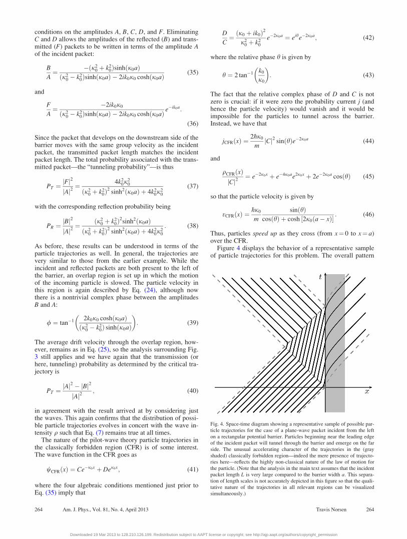
Figure 4 displays the behavior of a representative sampleof particle trajectories for this problem. The overall pattern

Fig. 4. Space-time diagram showing a representative sample of possible par-

ticle trajectories for the case of a plane-wave packet incident from the left

on a rectangular potential barrier. Particles beginning near the leading edge

of the incident packet will tunnel through the barrier and emerge on the far

side. The unusual accelerating character of the trajectories in the (gray

shaded) classically forbidden region—indeed the mere presence of trajecto-

ries here—reflects the highly non-classical nature of the law of motion for

the particle. (Note that the analysis in the main text assumes that the incident

packet length L is very large compared to the barrier width a. This separa-

tion of length scales is not accurately depicted in this figure so that the quali-

tative nature of the trajectories in all relevant regions can be visualized

simultaneously.)

264 Am. J. Phys., Vol. 81, No. 4, April 2013 Travis Norsen 264

Downloaded 19 Mar 2013 to 128.210.126.199. Redistribution subject to AAPT license or copyright; see http://ajp.aapt.org/authors/copyright_permission

is similar to the case of scattering from the step potential—particles that begin near the trailing edge of the incidentpacket will be swept up by the reflected packet before reach-ing x¼ 0, while those that begin nearer the leading edge ofthe incident packet will reach the barrier, tunnel across it,and emerge with the transmitted packet.

V. DISCUSSION

We have analyzed two standard textbook cases of one-dimensional quantum mechanical scattering and tunnelingfrom the point of view of the de Broglie-Bohm pilot-wavetheory. In particular, we have shown how the standard text-book expressions for the reflection and transmission/tunnel-ing probabilities—calculated using infinitely-extendedplane-wave states—can instead be understood as arisingfrom a certain type of idealized, non-Gaussian incident wavepacket. We then took advantage of this “plane-wave packet”approach to generate a tractable, indeed quite simple, pictureof how the particle trajectories in the pilot-wave theorydevelop.

It is hoped that the plane-wave packet approach mightprove clarifying for students learning standard textbookquantum mechanics. It is also hoped that introducing thepilot-wave theory through standard textbook examples willmake it easier for teachers to present the range of availableinterpretive options clearly and effectively to students.Recent work has shown that modern physics students haveparticular difficulty with conceptual questions involvingissues of interpretation,14 a finding that is hardly surprisinggiven that physics teachers themselves have divergent viewson interpretive questions and their place in the curriculum.15

These questions deserve to be discussed more explicitly andmore carefully, and it seems natural to do so in the contextof the kinds of example problems that students encounter insuch courses anyway.

Despite its not being suggested as an option in the text-book or lectures, several of the students interviewed in Ref.15 seem to have independently developed a pilot-wave typeunderstanding of single-particle interference phenomena.Many eminent physicists have also found a pilot-wave ontol-ogy to be the natural way to account for puzzling quantumeffects. Here, for example, is Bell on single-particle interfer-ence experiments:

“While the founding fathers agonized over the question”

‘particle’ or ‘wave’

de Broglie in 1925 proposed the obvious answer

‘particle’ and ‘wave’.

“Is it not clear from the smallness of the scintillationon the screen that we have to do with a particle?And is it not clear, from the diffraction andinterference patterns, that the motion of the particleis directed by a wave? De Broglie showed in detailhow the motion of a particle, passing through justone of two holes in [the] screen, could be influencedby waves propagating through both holes. And soinfluenced that the particle does not go where thewaves cancel out, but is attracted to where theycooperate. This idea seems to me so natural andsimple, to resolve the wave-particle dilemma in

such a clear and ordinary way, that it is a great mys-tery to me that it was so generally ignored.”16

In an earlier paper, Bell asked:

“Why is the pilot wave picture ignored in textbooks? Should it not be taught, not as the only way,but as an antidote to the prevailing complacency? Toshow that vagueness, subjectivity, and indeterminismare not forced on us by experimental facts, but bydeliberate theoretical choice?”17

If current physicists answered these questions, the majoritywould probably cite two factors, both of which involve someconfusion and mis-information. First, there is the oft-repeatedcharge that the pilot-wave theory involves an ad hoc and cum-bersome additional field—the so-called “quantum potential”—to guide the particle. The theory has indeed been presented insuch a form by Bohm and others.11,12 But as the examples inthe body of the present work should help make clear, this is anentirely unnecessary addition to the “minimalist” pilot-wavetheory, in which the field guiding the particle is none otherthan the usual quantum mechanical wave function obeying theusual Schr€odinger equation.

The second factor typically cited by critics of the pilot-wave theory is its non-local character and the associatedalleged incompatibility with relativity. It is true, as discussedjust after Eq. (5), that the pilot-wave theory is explicitly non-local. What the critics forget, however, is that ordinary quan-tum mechanics is also a non-local theory: already in itsaccount of the simple one-particle scattering phenomena dis-cussed here, orthodox quantum theory needs additional pos-tulates—in particular the infamous and manifestly non-localcollapse postulate—to explain what is empirically observed.The truth is that, as we know from Bell, no local theory canbe empirically adequate.4 So rejecting candidate interpreta-tions on the basis of their non-local character is hardlyappropriate. Nevertheless, it is interesting that the conven-tional wisdom on this point is completely backwards: thepilot-wave theory is actually less non-local than ordinaryquantum theory in the sense that it (unlike the orthodoxtheory) can at least account for the results of one-particlescattering/tunneling/interference experiments in a com-pletely local way.

It is thus hoped not only that the examples presented herewill provide a simple concrete way for the alternative pilot-wave picture to be introduced to students but also that theexamples will help to overturn some unfortunate and widelyheld misconceptions about the theory. And of course itshould be noted that the pilot-wave theory is just one of sev-eral alternatives to the usual Copenhagen-inspired theorythat appears in most textbooks. There is, for example, alsothe many-worlds (“Everettian”) theory, the spontaneous col-lapse (“GRW”) theory, the consistent (or decoherent) histor-ies approach, and many others. As someone who thinks thatthese questions—about the physics behind the quantum for-malism—are meaningful, important, fascinating, controver-sial, and too-often hidden under a shroud of unspeakability, Iwould like to see all of these interpretations more widelyunderstood and discussed by physicists, both in and out ofthe classroom. (Some suggestions for introducing the issuesand options to students can be found in Ref. 18.) At the endof the day, though, I cannot help but agree with Bell, who,after reviewing “Six possible worlds [i.e., interpretations] of

265 Am. J. Phys., Vol. 81, No. 4, April 2013 Travis Norsen 265

Downloaded 19 Mar 2013 to 128.210.126.199. Redistribution subject to AAPT license or copyright; see http://ajp.aapt.org/authors/copyright_permission

quantum mechanics,” concluded that “the pilot wave pictureundoubtedly shows the best craftsmanship.”16 Hopefully, theexamples discussed above will help others appreciate why.

ACKNOWLEDGMENTS

Thanks to Shelly Goldstein, Doug Hemmick, and twoanonymous referees for helpful comments on earlier draftsof the paper.

a)Electronic mail: tnorsen@smith.edu1An English translation of Louis de Broglie’s 1927 pilot-wave theory can be

found in G. Bacciagalluppi and A. Valentini, Quantum Theory at the Cross-roads (Cambridge University Press, Cambridge, 2009). David Bohm’s 1952

re-discovery of the theory is presented in “A Suggested Interpretation of the

Quantum Theory in terms of Hidden Variables, I and II,” Phys. Rev. 85,

166–193 (1952). A more contemporary overview, with further references,

can be found online at <plato.stanford.edu/entries/qm-bohm>.2J. S. Bell, “Beables for Quantum Field Theory” (1984) in Speakable andUnspeakable in Quantum Mechanics, 2nd ed. (Cambridge University

Press, Cambridge, 2004).3See, for example, R. G. Newton, Scattering Theory of Waves and Par-ticles, 2nd ed. (Springer, Berlin/Heidelberg/New York, 1982); M. Reed

and B. Simon, Methods of Modern Mathematical Physics III: ScatteringTheory (Academic Press, San Diego, 1979).

4J. S. Bell, “On the Einstein-Podolsky-Rosen Paradox,” Phys. 1, 195–200

(1964). Reprinted in Bell, 2004, in Speakable and Unspeakable in Quan-tum Mechanics, 2nd ed. For a contemporary systematic review of Bell’s

Theorem, see S. Goldstein, T. Norsen, D. Tausk, and N. Zanghi, “Bell’s

Theorem” online at <www.scholarpedia.org/article/Bell%27s_theorem>.5D. D€urr, S. Goldstein, and N. Zanghi, “Quantum equilibrium and the ori-

gin of absolute uncertainty,” J. Stat. Phys. 67, 843–907 (1992).6M. D. Towler, N. J. Russell, and A. Valentini, “Time scales for dynamical

relaxation to the Born rule,” Proc. R. Soc. London, Ser. A 468, 990–1013

(2012).7J. S. Townsend, Quantum Physics: A Fundamental Approach to ModernPhysics (University Science Books, Sausalito, CA, 2010).

8D. J. Griffiths, Introduction to Quantum Mechanics (Prentice-Hall, New

Jersey, 1995), p. 58.9R. Shankar, Principles of Quantum Mechanics, 2nd ed. (Springer, New

York, 1994).10C. Dewdney and B. J. Hiley, “A quantum potential description of one-

dimensional time-dependent scattering from square barriers and square

wells,” Found. Phys. 12, 27–48 (1982).11D. Bohm and B. J. Hiley, The Undivided Universe (Routledge, London

and New York, 1993), pp. 73–78.12P. Holland, The Quantum Theory of Motion (Cambridge University Press,

Cambridge, 1993), pp. 198–203 (and references therein).13For a rather different (alternative) approach to scattering that also uses the

terminology “plane-wave packet” see Stuart C. Althorpe, “General time-

dependent formulation of quantum scattering theory,” Phys. Rev. A 69,

042702-1–12 (2004).14S. Wuttiprom, M. D. Sharma, I. D. Johnston, R. Chitaree, and C. Soank-

wan, “Development and use of a conceptual survey in introductory quan-

tum physics,” Int. J. Sci. Educ. 31, 631–654 (2009).15C. Baily and N. D. Finkelstein, “Refined characterization of student per-

spectives on quantum physics,” PRST-PER 6, 020113-1–11 (2010).16J. S. Bell, “Six possible worlds of quantum mechanics,” 1986, reprinted in

Bell, 2004, in Speakable and Unspeakable in Quantum Mechanics, 2nd

ed. (Note: ellipsis in original.)17J. S. Bell, “On the impossible pilot wave,” 1982, reprinted in Bell, 2004, in

Speakable and Unspeakable in Quantum Mechanics, 2nd ed.18Bell’s paper, “Six Possible Worlds of Quantum Mechanics,” op. cit.,

reviews the relevant phenomena of single-particle interference and then

surveys six different extant interpretations. It is an extremely accessible

introduction to the nature (and existence) of the controversies, and I have

often used it as the basis for a one-class-period discussion in a sophomore-

level modern physics course. At a slightly more technical level, Sheldon

Goldstein’s two-part Physics Today article [March, 1998, pp. 42–46 and

April, 1998, pp. 38–42] gives an extremely clear presentation of three

attempts to formulate a “Quantum Theory Without Observers” and an illu-

minating explanation of why such a thing should be desirable in the first

place. For students who want to explore foundational issues (EPR, Bell,

etc.) and their emerging applications (quantum cryptography, computation,

etc.) in more depth, I would recommend GianCarlo Ghirardi’s lucid book,

Sneaking a Look at God’s Cards, Revised Edition, Gerald Malsbary, trans.

(Princeton U.P., 2005).

266 Am. J. Phys., Vol. 81, No. 4, April 2013 Travis Norsen 266

Downloaded 19 Mar 2013 to 128.210.126.199. Redistribution subject to AAPT license or copyright; see http://ajp.aapt.org/authors/copyright_permission