The Planning and Optimisation of DVB-H Radio...

9HSTFMG*aeaaia+

ISBN: 978-952-60-4009-7 (pdf) ISBN: 978-952-60-4008-0 ISSN-L: 1799-4934 ISSN: 1799-4942 (pdf) ISSN: 1799-4934 Aalto University

Department of Communications and Networking aalto.fi

BUSINESS + ECONOMY ART + DESIGN + ARCHITECTURE SCIENCE + TECHNOLOGY CROSSOVER DOCTORAL DISSERTATIONS

Aalto-D

D 4

/2011

The aim of this doctoral dissertation is to investigate advanced DVB-H radio network planning and optimisation. This dissertation presents the results of measurement techniques, network coverage and quality estimation, technological and economical optimisation, as well as error correction and single frequency network performance. The outcome includes proposed DVB-H radio network planning and optimisation methods that can be applied to the further investigation of detailed parameters in the radio link budget. There are also case studies that show the functionality of the presented methods with typical performance values.

Jyrki T. J. Penttinen T

he Planning and Optim

isation of DV

B-H

Radio N

etwork

Aalto

Unive

rsity

Department of Communications and Networking

The Planning and Optimisation of DVB-H Radio Network

Jyrki T. J. Penttinen

DOCTORAL DISSERTATIONS

School of Electrical Engineering

i

Preface

The idea of this thesis took a concrete form after I had worked in various DVB-H related pro-jects, including pre-FinPilot in Helsinki, Finland with TeliaSonera during 2004, and technical DVB-H trialling in USA with Nokia and Nokia Siemens Networks during 2007, among other smaller scale DVB-H radio network planning tasks I carried out in the international level. I also had chance to participate in the specification work of DVB-H Technical Module in 2004. As a result of these activities, I started to consider selected study items about the radio network planning and optimisation of DVB-H. As my main idea was to carry out an overall revision of the DVB-H planning, it was logical to divide the work into separate study items, process them in the format of sub-publications and write the thesis as an article dissertation.

The purpose of this thesis is to study the most relevant items that have effect on the radio plan-ning of DVB-H. For the selection of the study items, I designed a planning and optimisation process chart. The actual investigation is based on the DVB-H field tests, simulations and litera-ture studies about the radio network planning.

I express my warmest gratitude to my supervisor Professor Sven-Gustav Häggman and my in-structor Dr. Jukka Henriksson for the fruitful discussions and feedback. I thank my reviewers Professor Jens Zander and Professor Jukka Lempiäinen for the prompt work and most useful comments. I am honoured for having Professor Jens Zander and Professor Markku Renfors as my opponents. I thank my colleagues at Nokia, Nokia Siemens Networks, TeliaSonera, FinPilot trial group and DVB-H Technical Module for all the DVB-H discussions. I want to express my special thanks to Pekka H. K. Talmola, Petri Jolma, Juha Viinikainen, Tommi Auranen, Eric Kroon, Jouni Oksanen, Pekka Pesari, Anssi Korkeakoski, Francesco Calabrese, Ernst-Otto Afflerbach, Stefan Schneiders, Jesús Fernandez, Juha Jäntti, Jussi Brannfors, Dario Ambrosini and Paul Hartman. I thank my DVB-H teams in USA, Mexico and Finland, as those activities actually triggered the investigations of this thesis. I also want to thank Timo Kajamaa and Jouko Rautio for taking care of my initial ��ing to the investigation work back in 90's.

I would like to express my gratitude to Nokia Siemens Networks for the support. I give special thanks to the Foundation of the Finnish Society of Electronics Engineers (Elektroniikkainsinöö-rien säätiö), the Foundation of Ulla Tuominen (Ulla Tuomisen säätiö) and the Nokia Foundation for the scholarships which made it possible to carry out the task during my spare time.

Finally, I want to thank my close family, Katriina, Pertti, Aune, Elva, Stephanie, Carolyne and Miguel, for all the support and patience during the work.

Madrid, Spain, 17 January 2011 Jyrki T.J. Penttinen

ii

iii

Contents

Preface........................................................................................................................................... i

Contents ...................................................................................................................................... iii

List of Publications.................................................................................................................... vii

List of Abbreviations.................................................................................................................. ix

List of Symbols .......................................................................................................................... xv

List of Figures........................................................................................................................... xxi

List of Tables ........................................................................................................................... xxv

1 Introduction.......................................................................................................................... 1 1.1 DVB-H scene............................................................................................................... 1 1.2 DVB-H radio network planning references ................................................................. 2 1.3 Problem identification ................................................................................................. 4

1.3.1 Radio network planning process .................................................................... 4 1.3.2 Cost impact..................................................................................................... 4 1.3.3 Single frequency network performance.......................................................... 4 1.3.4 Field test and analysis methodology............................................................... 5 1.3.5 Coverage planning.......................................................................................... 6

1.4 Objectives of the thesis ................................................................................................ 7 1.5 Contributions of the thesis ........................................................................................... 7 1.6 Thesis outline............................................................................................................. 12

2 Principles of DVB-H .......................................................................................................... 13 2.1 Description................................................................................................................. 13 2.2 DVB-H network......................................................................................................... 16

2.2.1 Architecture .................................................................................................. 16 2.2.2 Functionality................................................................................................. 17 2.2.3 Elements ....................................................................................................... 19

iv

2.3 Radio functionality .................................................................................................... 20 2.3.1 Radio transmitter .......................................................................................... 20 2.3.2 Terminal ....................................................................................................... 20 2.3.3 Frequency ..................................................................................................... 21 2.3.4 OFDM parameters........................................................................................ 22 2.3.5 Error recovery............................................................................................... 25 2.3.6 Time Slicing ................................................................................................. 29 2.3.7 SFN / MFN................................................................................................... 30 2.3.8 Interaction channel ....................................................................................... 32

3 Initial radio network planning process ............................................................................ 35 3.1 High-level network dimensioning process ................................................................ 35 3.2 Capacity planning ...................................................................................................... 37

3.3 Coverage and QoS planning [Publications V, VII] ................................................... 41 3.3.1 Radio link budget ......................................................................................... 41 3.3.2 Propagation models ...................................................................................... 50

3.4 Safety distance [Publication VI] ................................................................................ 52

3.5 Cost prediction [Publication I]................................................................................... 54

4 Detailed radio network design .......................................................................................... 59 4.1 Identifying the planning items ................................................................................... 59 4.2 Detailed network planning process............................................................................ 60 4.3 Capacity planning ...................................................................................................... 62

4.4 Coverage planning [Publications V, VII] .................................................................. 62 4.4.1 Effect of site locations.................................................................................. 62 4.4.2 Site cell range predictions ............................................................................ 63

4.5 Local measurements [Publications II, VIII, IX] ........................................................ 64 4.5.1 Coverage area ............................................................................................... 66 4.5.2 Error correction ............................................................................................ 67 4.5.3 Accuracy of error correction analysis........................................................... 69

4.6 Effect of SFN [Publications III, IV, X] ..................................................................... 73 4.6.1 Non-interfered network ................................................................................ 74 4.6.2 Interfered network ........................................................................................ 80 4.6.3 Conclusion.................................................................................................... 86

v

4.7 Radiation limitations [Publication VI]....................................................................... 87

4.8 Cost prediction [Publication I]................................................................................... 89

5 Optimisation ....................................................................................................................... 91 5.1 Site parameters........................................................................................................... 91

5.1.1 Controlled SFN interference [Publications III, X] ....................................... 91

5.1.2 SFN gain and interferences [Publications IV, VII, X] ................................. 93

5.1.3 MPE-FEC gain [Publications II, VIII, IX] ................................................... 97

5.1.4 Antenna down-tilt [Publication V] ............................................................. 103 5.2 User experience related parameters ......................................................................... 104

5.3 Cost optimisation [Publication I] ............................................................................. 105 5.3.1 Cost optimisation in non-interfered network.............................................. 105 5.3.2 Cost optimisation in interfered SFN network............................................. 108

6 Summary and conclusions............................................................................................... 119 6.1 Main results of this thesis ........................................................................................ 119 6.2 Usability of the results ............................................................................................. 120 6.3 Further study items .................................................................................................. 121

References ................................................................................................................................ 123

Errata ....................................................................................................................................... 133

Appendix A: SFN Simulator

Appendix B: Publications I � X

vii

List of Publications

This thesis contains a summary of the following Publications which are referred to in the text by their Roman numerals. These Publications were presented in conferences or journals during 2008–2009.

I Jyrki T. J. Penttinen. CAPEX and OPEX optimisation as function of DVB-H trans-mitter power. The Third International Conference on Digital Telecommunications ICDT 2008. International Academy, Research, and Industry Association (IARIA). June 29�July 5, 2008. Bucharest, Romania. Pages 140�145.

II Jyrki T. J. Penttinen. Field measurement and data analysis method for DVB-H mo-bile devices. The Third International Conference on Digital Telecommunications ICDT 2008. International Academy, Research, and Industry Association (IARIA). June 29�July 5, 2008. Bucharest, Romania. Pages 146�151.

III Jyrki T. J. Penttinen. The simulation of the interference levels in extended DVB-H SFN areas. The Fourth International Conference on Wireless and Mobile Communi-cations ICWMC 2008. International Academy, Research, and Industry Association (IARIA). July 27�August 1, 2008. Athens, Greece. Pages 223�228.

IV Jyrki T. J. Penttinen. The SFN gain in non-interfered and interfered DVB-H net-works. The Fourth International Conference on Wireless and Mobile Communica-tions ICWMC 2008. International Academy, Research, and Industry Association (IARIA). July 27�August 1, 2008. Athens, Greece. Pages 294�299.

V Jyrki T. J. Penttinen. DVB-H coverage estimation in highly populated urban area. The 58th Annual IEEE Broadcast Symposium, October 15�17, 2008. Alexandria, VA, USA. 6 pages.

VI Jyrki T. J. Penttinen. DVB-H radiation aspects. The IEEE International Symposium on Wireless Communication Systems ISWCS 2008, October 21–24, 2008. Reykja-vik, Iceland. Pages 258�262.

VII Jyrki T. J. Penttinen. DVB-H performance simulations in dense urban area. The Third International Conference on Digital Society ICDS 2009. International Acad-emy, Research, and Industry Association (IARIA). February 1�7, 2009. Cancun, Mexico. Pages 83�88.

viii

VIII Jyrki T. J. Penttinen and Eric Kroon. MPE-FEC performance as function of the terminal speed in typical DVB-H radio channels. The IEEE International Symposium on Broadband Multimedia Systems and Broadcasting (BMSB). 13�15 May, 2009, Bilbao, Spain. 6 pages.

IX Jyrki T. J. Penttinen. Field measurement and data analysis method for DVB-H mo-bile devices. International Journal on Advances in Systems and Measurements. Inter-national Academy, Research, and Industry Association (IARIA). ISSN 1942�261x, Vol. 2, No. 1, year 2009. Pages 18–32.

X Jyrki T. J. Penttinen. The SFN gain in non-interfered and interfered DVB-H net-works. International Journal on Advances in Internet Technology. International Academy, Research, and Industry Association (IARIA). ISSN 1942�2652, Vol. 2, No. 1, 2009. Pages 115–134.

The author has contributed solely all the contents of the Publications I�VII and IX�X, including the creation of the simulator explained in Appendix 1. For Publication VIII, the author contrib-uted 50 % of the contents which included the theoretical revision, laboratory and indoor live network measurements and data collection, as well as the respective analysis and conclusions. The summary of the above mentioned Publications is presented in Chapters 4�6 and all the Publications are annexed in originally presented format.

ix

List of Abbreviations

16-QAM Quadrature Amplitude Modulation (with 16 constellation points)

2D Two-dimensional

2K FFT mode of OFDM

3D Three-dimensional

3G Third Generation

4K FFT mode of OFDM

64-QAM Quadrature Amplitude Modulation (with 64 constellation points)

8K FFT mode of OFDM

AAA Authentication, Authorisation and Accounting

AAC Advanced Audio Coding

ADSL Asymmetric Digital Subscriber Line

ADT Application Data Table

AWGN Additive White Gaussian Noise

BMCOFORUM Broadcast Mobile Convergence Forum

CAPEX Capital Expenditure

CBMS Convergence of Broadcasting and Mobile Services

CDF Cumulative Distribution Function

CELTIC Services to Wireless, Integrated, Nomadic, GPRS, UMTS & TV handheld terminals.

CINR Carrier and Interference to Noise Ratio, C/(N+I)

COFDM Coded Orthogonal Frequency Division Multiplex

x

CR Code Rate

CRC Cyclic Redundancy Check

DTTV Digital Terrestrial TV

DVB Digital Video Broadcasting

DVB-C Digital Video Broadcasting, Cable

DVB-H Digital Video Broadcasting, Handheld

DVB-NGH Digital Video Broadcasting, Next Generation Handheld

DVB-S Digital Video Broadcasting, Satellite

DVB-T Digital Video Broadcasting, Terrestrial

EIRP Effective Isotropic Radiated Power

EMC Electro-Magnetic Compatibility

ERP Effective Radiated Power

ES Elementary Stream

ESG Electronic Service Guide

ETSI European Telecommunications Standards Institute

EU European Union

FEC Forward Error Correction

FER Frame Error Rate

FFT Fast Fourier Transform

GI Guard Interval

GPS Global Positioning System

GSM Global System for Mobile communications

HP High Priority stream

xi

HW Hardware

I/Q In phase (I) and Quadrature (Q) signal components

IMSI International Mobile Subscriber Identity

IP Internet Protocol

IPDC IP Datacast

IPE IP Encapsulator

ITU-R International Telecommunication Union, Radio section

LAN Local Area Network

LOS Line-of-Sight

LP Low Priority stream

LTE Long Term Evolution

MBMS Mobile Broadcast / Multicast Service

MER Modulation Error Rate

MFER Frame Error Rate after MPE-FEC

MFN Multi Frequency Network

MMS Multimedia Messaging Service

MIMO Multiple Input Multiple Output

Motivate Mobile Television and Innovative Receivers project

MPE Multi-Protocol Encapsulation

MPE-FEC Multi-Protocol Encapsulation ⎯ Forward Error Correction

MPEG-2 Moving Pictures Expert Group 2

MS Mobile Station

MUX Multiplexer

xii

N/A Non-applicable

N-LOS Non-Line-of-Sight

OFDM Orthogonal Frequency Division Multiplex

OMS Operations and Maintenance System

OPEX Operating Expenditure

PDF Probability Density Function

PID Program Identifier

PSI Program Specific Information

PTM Point-to-Multipoint

PTP Point-to-Point

QEF Quasi Error-Free

QoS Quality of Service

QPSK Quadrature Phase Shift Keying (with four constellation points)

RF Radio Frequency

ROI Return of Investment

RS Reed-Solomon coding

RSSI Received Signal Strength Indicator

RX Receiver

SER SFN Error Rate

SFN Single Frequency Network

SI Service Information

SIM Subscriber Identity Module

SMS Short Message Service

xiii

Stdev Standard Deviation

TDMA Time Division Multiple Access

TPS Transmitter Parameter Signalling

TS Transport Stream

TX Transmitter

UHF Ultra High Frequency band

UMTS Universal Mobile Telecommunications System

VHF Very High Frequency band

WiMAX Worldwide Interoperability for Microwave Access

WLAN Wireless Local Area Network

xv

List of Symbols

� Alpha parameter expressing the hierarchical constellation shape

� Angle of the position of the DVB-H terminal (rad)

ε Safety margin of antenna feeder power (W)

)(tkφ OFDM subcarrier in time domain

π Pi ≈ 3.14159265 (constant)

ωk Frequency of the orthogonal subcarrier k (Hz)

Standard deviation (dB)

A Area (km2)

Atot Area, whole investigated (km2)

Acell Area, site cell coverage (km2)

a(hMS)LC Area type factor in Okumura-Hata path loss prediction model for large city

a(hMS)SMC Area type factor in Okumura-Hata path loss prediction model for small and medium city

B Bandwidth, receiver noise (Hz)

Bch Bandwidth, channel (MHz)

C Carrier level (dB)

commonC Costs, site dependent fixed common items (currency unit)

siteC Costs, total of the DVB-H site (currency unit)

totC Costs, total of the DVB-H network (currency unit)

CtotC Costs, total of CAPEX (currency unit)

OyeartotC / Costs, total of OPEX per year (currency unit)

xvi

iableCvar Costs, site dependent variable items (currency unit)

C/(N+I) Carrier to noise and interference level ratio (dB)

C/N Carrier to noise level ratio (dB)

(C/N)min Carrier to noise level ratio, minimum functional (dB)

C1 Carrier, reference (dB)

Ctot Sum of all received carriers (dB)

ce Cost of electricity (currency unit / kWh)

(cn)min Carrier to noise, minimum C/N requirement (dB)

Deff Difference of the arriving signals, effective distance (km)

DSFN Maximum allowed inter-site distance (diameter) within SFN area (km)

d Maximum distance (km)

dcell Radius of the site cell (km2)

delta-T Time for the beginning of the next time sliced burst (s)

E Number of errors (positive integer)

Ein_average Field strength, average in indoors (dBμV/m)

Emin(in) Field strength, minimum in indoors (dBμV/m)

Emin(out) Field strength, minimum in outdoors (dBμV/m)

Eout_average Field strength, average in outdoors (dBμV/m)

F Noise figure (dB)

Ferr_am Erroneous frames after MPE-FEC (positive integer)

Ferr_bm Erroneous frames before MPE-FEC (positive integer)

Fr Total number of received frames (positive integer)

FER Frame Error Rate (%)

xvii

FER1 The presence of a remaining frame error

FER5 Frame Error Rate limit of 5%

f Frequency (MHz)

fk Frequency of the subcarrier number k (Hz)

fN OFDM carrier (order number N)

Gant Gain, mobile station antenna (dBi)

GMPE-FEC Gain, MPE-FEC (dB)

GRX Gain, receiver antenna (dBi)

GSFN Gain, SFN (dB)

GTX Gain, transmitter antenna (dBi)

ht(t) Channel impulse response

hBS Height of the transmitter antenna of DVB-H site (m)

hMS Height of the DVB-H receiver (m)

I Interference level (dB)

Itot Sum of all interferences (dB)

K Reuse factor in hexagonal site cell layout (positive integer)

k Boltzmann’s constant 1.38·10-23 (J/K), or number of data symbols per block (positive integer), or positive integer in SFN reuse pattern formula (variable)

Lant Loss, antenna (dB)

Lb Loss, building (dB)

Lcc Loss, cable and connectors (dB)

LGSM Loss, GSM filter (dB)

Llv Loss, location variation (dB)

xviii

Lmax Loss, maximum path for the carrier (dB)

Lmaxinterference Loss, maximum path for the interfering signal (dB)

Lnorm Loss, fading caused by the long-term variations (dB)

Lopen Loss, Okumura-Hata path loss prediction for open area (dB)

Lpl(in) Loss, maximum path loss in indoors (dB)

Lpl(out) Loss, maximum path loss in outdoors (dB)

Lps Loss, power splitter (dB)

Lsub-urban Loss, Okumura-Hata path loss prediction for sub-urban area (dB)

LRayleigh Loss, fading caused by the short-term variations (dB)

LND Distribution for the long-term fading (table variable)

Locprob Location probability, area (%)

l Positive integer in SFN reuse pattern formula (variable)

MFER Frame Error Rate after MPE-FEC (%)

MFER1 The presence of a remaining frame error after MPE-FEC

MFER5 Frame Error Rate limit of 5% after MPE-FEC

m Number of bits in symbol (positive integer)

N Number of carriers in OFDM (positive integer)

Nsites Number of the sites in SFN (positive integer)

Ncells Number of the site cells of DVB-H network (positive integer)

Ny Number of the years (positive real number)

ND Distribution for fast fading (table variable)

Noisefloor Noise floor including noise limit and receiver’s noise figure (dBm)

xix

n Total number of m-bit symbols in the encoded blocks (positive integer), or amount of samples (positive integer)

totCP Total useful received power (W)

Pc Electrical power consumption (W)

totIP Total received power of the interfering components (W)

Pi Power, isotropic (dBm)

Pmin(in) Power, minimum required in indoors (dBm)

Pmin(out) Power, minimum required in outdoors (dBm)

Pn Noise floor (dBm)

PRX Received power level (dBm)

)(CPRX Received useful carrier power level (dBm)

)(IPRX Received interfering power level (dBm)

PRXmin Sensitivity, receiver (dBm)

PRXref Reference power level (dBm)

PTX Transmitter output power (dBm)

PTX,opt Optimal radiating power as a result of CAPEX / OPEX analysis (dBm)

PTX,reg Maximum radiating power as a result of regulatory limits (dBm)

PTX,safety Maximum radiating power as a result of EMC / radiation safety analysis (dBm)

effectiveTXP Transmitter power after the filter loss (dBm)

Ptx Power level, radiating power in EIRP (dBm)

R Sampling resolution (%)

r Site cell radius of the carrier C (km)

rinterference Site cell radius of the interfering site (km)

xx

S Number of erasures in the block (positive integer)

s(t) OFDM signal in time domain

T Temperature (Kelvin)

TF Time, frame duration (s)

TGI Time, Guard Interval duration (s)

TS Symbol duration of OFDM (s)

TU Time, useful symbol duration (s)

t Parameter in RS-coding (variable), or time (s)

tmax Maximum operating time of DVB-H network (years)

x Simulation area, x-coordinate point (km)

x Loss, average (dB)

xk Data symbol number k

olx Overlapping portion of the site cells in x-axis (%)

x1km Simulation area, x-coordinate, upper left corner point (km)

x2km Simulation area, x-coordinate, lower right corner point (km)

xkm Simulation area, total length of x-axis (km)

y Simulation area, y-coordinate point (km)

y1km Simulation area, y-coordinate, upper left corner point (km)

y2km Simulation area, y-coordinate, lower right corner point (km)

ykm Simulation area, total length of y-axis (km)

oly Overlapping portion of the site cells in y-axis (%)

xxi

List of Figures

Figure 2-1. The DVB-CBMS architecture as interpreted from [Dvb09]. ................................... 16 Figure 2-2. The complete DVB-H delivery chain can be divided into the core network (DVB-IPDC) and the radio network (DVB-H). ..................................................................................... 17 Figure 2-3. It is possible to multiplex DVB-H IP streams with DVB-T MPEG-streams. These streams can be delivered via a common infrastructure for DVB-H and DVB-T terminals. ....... 18 Figure 2-4. The high-level block diagram of the DVB-H receiver. The RF signal is directed to the input of the demodulator, and the output is further handled by the DVB-H terminal........... 18 Figure 2-5. The DVB-H reference receiver................................................................................. 21 Figure 2-6. The frame structure of DVB-H................................................................................. 22 Figure 2-7. OFDM is based on orthogonal subcarriers containing the useful data (marked with light grey colour) as well as pilot signals (marked with dark grey colour). ................................ 23 Figure 2-8. The principle of I/Q constellations of DVB-H. ........................................................ 24 Figure 2-9. The DVB-H error protection scheme. ...................................................................... 26 Figure 2-10. The MPE-FEC frame consists of the application data table for IP datagrams and the RS data table for RS parity bytes. ............................................................................................... 27 Figure 2-11. The principle of the Time Slicing functionality. .................................................... 30 Figure 2-12. The summing of the separate multi-path components can be done in the useful time window TU whilst all the components occur within the time delay TGI determined by the guard interval......................................................................................................................................... 31 Figure 2-13. The principle of overlapping GSM/UMTS coverage areas. ................................... 33 Figure 3-1. The high-level cross-relations of the most relevant DVB-H radio network planning items. ........................................................................................................................................... 35 Figure 3-2. The proposed radio network planning process in the initial phase. The process contains high-level estimations of the capacity and coverage by taking into account the economical and regulatory limitations. ....................................................................................... 36 Figure 3-3. An example of the typical building loss in a format of a cumulative RSSI histogram, which is obtained by the difference of the received power in the indoor and outdoor area. This case represents the deep building type of B2. ............................................................................. 46 Figure 3-4. Examples of the DVB-H site cell radius, when 16-QAM, CR 1/2 and MPE-FEC 1/2 are applied. Neither the SFN gain nor MPE-FEC gain are utilised in these calculations. .......... 51 Figure 3-5. An example of the transmitter cost in terms of a single watt as a function of the total power level. ................................................................................................................................. 54 Figure 4-1. The cross relations of the items affecting on the DVB-H radio dimensioning. In this diagram, the final aim is the balancing of the capacity and coverage by taking into account the restrictions and enhancements related to the technology, commercial and regulatory items...... 60

xxii

Figure 4-2. The detailed planning phase contains in-depth analysis of the effects of the performance parameters. The steps can be iterative.................................................................... 61 Figure 4-3. Comparison of the RSSI display of 3 different DVB-H terminals used in Publication IX. Cumulative distribution of the laboratory measurement with 90 samples per terminal. ...... 65 Figure 4-4. An example of the collected received power levels by moving the receiver close to the functional cell edge. The received power level samples and corresponding geographical locations can be observed by post-processing the measurement data to a map format which indicates the expected coverage limits. ....................................................................................... 66 Figure 4-5. The first step of the proposed methodology arranges the occurred samples as a function of the received power level, showing the amount of error-free instances, occurred instances with frame errors that could be corrected with MPE-FEC, and remaining erroneous frames after MPE-FEC................................................................................................................ 68 Figure 4-6. The method shows the normalized number of occurred events per each RSSI........ 69 Figure 4-7. An amplified view to the 5% FER / MFER level..................................................... 69 Figure 4-8. An example of the collected data distribution over the RSSI scale.......................... 71 Figure 4-9. A view to the case result graph showing the FER and MFER curves with the respective error margin that is calculated for the absolute values of the samples for each RSSI category individually................................................................................................................... 72 Figure 4-10. An example of individually received signal levels in the same area, and their total power based on the direct power summing. The same terminal was utilized. ............................ 76 Figure 4-11. CDF of the 3 individual and summed signals presented in Figure 4-11................. 76 Figure 4-12. An example of the simulated area with the SFN reuse pattern size K=7................ 77 Figure 4-13. The SFN gain obtained via the simulations of Publication IV for the non-interfered network (QPSK, FFT 8K, GI 1/4). The comparable results of the studied references are also presented. .................................................................................................................................... 80 Figure 4-14. There are no interferences when the sites are within the SFN area even if the receiver drifts outside of the SFN area. The reception within this outer zone is thus possible whenever the minimum required C/N can still be reached.......................................................... 82 Figure 4-15. When the distance of two sites exceed the SFN limit, there occur interferences in those areas where Deff > DSFN. Figure shows the interference zone that applies for Deff > DSFN everywhere with the I-component greater than the noise floor. In this case, PTX is +70 dBm and the site antenna height is 80 m. The total area size is 45 km × 45 km. ....................................... 82 Figure 4-16. The distribution of the destructive interference. It can be seen that the useful field strength is sufficiently high close to the nearest site cell to avoid the destructive interferences, but otherwise this type of interference may occur anywhere within the interference zone. ....... 83 Figure 4-17. The geographical distribution of C/I when PTX = +70 dBm. .................................. 84 Figure 4-18. The effect of the interference can be seen when the power level is set to +80 dBm in this specific case. The reduced C/I-level can be seen clearly behind the sites within the interference zone on the left and right hand sides. ...................................................................... 84 Figure 4-19. PDF of the 2-site simulations (PTX = +70 dBm). .................................................... 85 Figure 4-20. CDF of the 2-site simulations for PTX of +70 dBm. Also comparison results with PTX of +60 dBm and +80 dBm sites are included........................................................................ 86

xxiii

Figure 5-1. The outcome of the simulations of the extended SFN area interferences. ............... 92 Figure 5-2. An example of the balancing of SFN gain and SFN interference level in long-term fading channel. K represents the SFN reuse pattern size, i.e. the number of sites within the SFN area. ............................................................................................................................................. 95 Figure 5-3. The simulation results of the SFN gain and interference balancing for the 16-QAM cases. ........................................................................................................................................... 96 Figure 5-4. An example of the simulation results in Mexico City layout with parameter set of B=6MHz, QPSK modulation, CR=1/2, MPE-FEC=1/2, GI=1/32 and FFT=8K in a combined long-term and Rayleigh fading channel. The map in left hand site represents the carrier distribution with noise level as reference, and the right one the interference distribution. The site circles indicate the height of the antennas................................................................................... 96 Figure 5-5. The C/(N+I) distribution of the previous example. .................................................. 97 Figure 5-6. An example of the cumulative distribution of occurred frame errors as a function of the received power level.............................................................................................................. 98 Figure 5-7. An example of the error recovery in case of the impulse noise................................ 99 Figure 5-8. Summary of FER5 and MFER5 analysis in a single site cell case. ........................ 100 Figure 5-9. Cost optimisation process in non-interfered DVB-H network. .............................. 106 Figure 5-10. Cost optimisation in interfered DVB-H network.................................................. 108 Figure 5-11. The cost effect of the DVB-H network when the antenna height is varied. This case includes relatively high transmission costs as utilized in Publication I. ................................... 115 Figure 5-12. An example of the cost effect as a function of the antenna height when the transmission costs are assumed to be low. ................................................................................ 116 Figure 6-1. PDF and CDF of the Rayleigh distribution. ........................................................... 135 Figure 6-2. The PDF of the comparative analysis of the power summing in squared and direct manner....................................................................................................................................... 137 Figure 6-3. The CDF of the power summing analysis. ............................................................. 137 Figure 6-4. Comparative simulation results for the SFN gain in the non-interfered environment by applying squared and direct power summing....................................................................... 139 Figure 6-5. The high-level block diagram of the simulator...................................................... A–1 Figure 6-6. Simulator’s initiation phase. .................................................................................. A–3 Figure 6-7. The principle of the fast and long-term fading in the receiving end...................... A–4 Figure 6-8. PDF and CDF of the normal distribution representing the variations of long-term loss when the standard deviation is set to 5.5 dB..................................................................... A–5 Figure 6-9. Example of the transmitter site locations the simulator has generated.................. A–7 Figure 6-10. The active transmitter sites are selected from the 2-dimensional site cell matrix with the individual numbers of the sites................................................................................... A–8 Figure 6-11. The x and y coordinates for the calculation of the site locations. ........................ A–8 Figure 6-12. The geometrical characteristics of the hexagonal model used in the simulator. . A–9

xxiv

Figure 6-13. The idea of the SFN reuse pattern. In this case, K=9. The colours represent different frequencies, each forming a single SFN area with 9 sites. ...................................... A–10 Figure 6-14. The simulation phase. ........................................................................................ A–12 Figure 6-15. The terminal is placed in the map varying the x and y coordinates, and the distance from the site antenna is calculated in 3D space...................................................................... A–13 Figure 6-16. The principle of the snap-shot of each simulation round. ................................. A–13 Figure 6-17. An amplified view to the outage probability of 10% (area location probability of 90 %) with respective C/(N+I) values for SFN reuse pattern size of K=1…16. ......................... A–18 Figure 6-18. The formed curve for the distances of 1–20 km of the mountain site is close to the logarithmic form, as used in Publication VII. ........................................................................ A–21 Figure 6-19. The interpolated curve for the distance of 20–100 km can be formed linearly. A–21 Figure 6-20. The error margin of the estimated path loss values obtained via the original tabulated values of the model ITU-R P.1546-3 and the respective regression curves is within +0.2…–0.5 dB up to 60 km of distance. There is also a peak up to +0.8 dB in close distance which does not have significance in this case. ....................................................................... A–22 Figure 6-21. The uniformity of the coordinate distribution can be analyzed by slicing the x-axis and y-axis of the investigated area in 10 sub-areas and revise the percentage of the occurred locations in each slice............................................................................................................. A–24 Figure 6-22. The graphical presentation of occurred x- and y-coordinates in the sub-slices of the area. ........................................................................................................................................ A–25 Figure 6-23. Comparison of the effect of the number of the simulation rounds per complete simulation. A total of 5 simulations are presented in each case. A part of the S-curve is shown around the 5 % FER point. ..................................................................................................... A–27 Figure 6-24. Cumulative presentation of the standard deviation classes per different lengths of the simulation. ........................................................................................................................ A–28

xxv

List of Tables

Table 2-1. The effect of the GI and FFT size as a function of the maximum tolerable signal delay and the longest non-interfering distance between transmitters within SFN. ..................... 25 Table 3-1. The summary of total DVB-H bitrates as a function of the parameter values as presented in [Dvb09]. The values for the 5 MHz band can be extrapolated from the others...... 37 Table 3-2. An example of the DVB-H link budget. .................................................................... 42 Table 3-3. The area location probability in the site cell edge and over the whole site cell area for the mobile reception when the standard deviation is 5.5 dB, according to [Dvb09]................... 43 Table 3-4. The estimated site cell radius for a set of transmitter antenna heights hBS and transmitter power levels PTX by applying the Okumura-Hata model for the urban area. ............ 55 Table 3-5. The total number of sites in the planned area. ........................................................... 56 Table 3-6. An example of the unit cost of the sites for a set of power categories....................... 56 Table 3-7. The normalized cost for different parameter values in order to cover 100×100 km2.57 Table 3-8. The summary of pros and cons of DVB-H transmitter power levels......................... 57 Table 4-1. An MPE-FEC error analysis for the example shown above. (* indicates too low sampling rate).............................................................................................................................. 72 Table 4-2. Numerical values of individual signals of the example. ............................................ 76 Table 4-3. The values of the summed signals of the example. GSFN is calculated by comparing the average and 50%-ile level with the strongest individual signal of each case. ....................... 77 Table 4-4. Comparison of the SFN gain values via different studies.......................................... 78 Table 5-1. The MPE-FEC gain for the investigated parameter values in a single site cell. ...... 101 Table 5-2. Comparison of indoor pedestrian MPE-FEC results obtained from Publication VIII and [Apa06b]............................................................................................................................. 103 Table 5-3. The most relevant CAPEX items and relations. ...................................................... 110 Table 5-4. Cable types and main characteristics utilized in the CAPEX/OPEX analysis of this thesis.......................................................................................................................................... 111 Table 5-5. An example of the site cell radius obtained by varying the cable type and transmitter power levels. N/A is shown if the cable is not suitable for the respective power level. ........... 113 Table 5-6. The most relevant OPEX items and relations. ......................................................... 113 Table 6-1. Comparison of the squared and direct power summing........................................... 136 Table 6-2. An example of simulation results, C/(N+I) as a function of the cumulative area location probability. A total of 7 complete simulations are presented, for the SFN reuse patterns K of 1, 3, 4, 7, 9, 12 and 16. ................................................................................................... A–17 Table 6-3. Comparison of the values obtained by interpolating the tabulated form and the regression curves. ................................................................................................................... A–22

xxvi

Table 6-4. The percentage of the samples in each sliced area of x-axis. The ideal distribution would result 10 % of samples in each slice. The table presents a total of 5 complete simulations with 60,001 rounds each......................................................................................................... A–24 Table 6-5. The percentile values as a function of y-axis slices. A total of five simulation rounds are presented........................................................................................................................... A–24 Table 6-6. The analysis of probability variations when C/I = 8.5 dB reference point is observed in each simulation. Table shows the respective variations in probability values. .................. A–26 Table 6-7. The analysis of the variations of the interpretation of C/I value when 5% probability point is observed. ................................................................................................................... A–26 Table 6-8. The accuracy analysis of the simulation cases...................................................... A–28

1

1 Introduction

1.1 DVB-H scene

The time and location independent mobile communications has changed our living style glob-ally. It is thus not surprising that the evolution of mobile technologies contains ever advanced solutions. In addition to the convergence of mobile communications with terminals capable of handling various simultaneous services and bearers like GSM, 3G and wireless LANs, also the importance of the broadcast based services is increasing.

Mobile broadcasting is a method that provides high channel capacity. It brings new aspects in the personal information handling, whether it is about leisure time with entertaining TV pro-grams or real-time news, economics and business related information delivery. This interactive mobile multimedia is one of the key ideas in the evolution of mobile communications. Public service broadcasters deliver television and audio programs over terrestrial, satellite and cable transmission increasingly in digital mode. It is foreseen that this program offer will be enhanced for the reception on mobile devices [Dvb06c, p. 21], meaning that the contents and format of the information source will be adapted to the small screen of the terminal and to the environment with high level of mobility.

This thesis concentrates on the Digital Video Broadcasting in Handheld environment (DVB-H). The advantage of the broadcast system over the mobile network's Point-to-Point streaming is that it provides the services in large areas without capacity limitations, i.e. the amount of the actively receiving users does not limit the transmitting capacity. The site cell coverage area of DVB-H is normally between that of traditional cellular systems and TV broadcast networks. DVB-H has adopted solutions from both TV broadcast and cellular systems. It is especially suitable for the mobile environment because it takes into account the varying radio conditions in both indoors and outdoors, it has a small screen size, relatively long battery life and it is able to cope with the varying velocities of the terminal. Various DVB-H element vendors, service providers and broadcasters are actively working in the field as [Dvb09] shows.

The system has been standardised in DVB-H sub-groups working under ETSI (European Tele-communications Standards Institute). The first complete DVB-H specification was published in 2004 which generated various trials and pilots. One of the first trial setups called FinPilot was initiated in Finland in 2005, and Italy was the first country to launch the commercial DVB-H service in 2007. The system is also supported by European Union. Nevertheless, DVB-H is not European specific, but it has been evaluated as a candidate in other continents like North and Latin America as well as in Asia [web02].

2

DVB-H belongs to the DVB family, other variations being DVB-T (terrestrial), DVB-C (cable) and DVB-S (satellite). DVB-H is based on the DVB-T standard, but DVB-H is designed spe-cifically for the moving environment. Within a DVB-H frequency band, which would be useful only for a single DVB-T channel at the time, it is possible to transmit several DVB-H sub-chan-nels containing video and/or audio. This is a result of relatively low bit stream capacity demand as the screen size and thus the resolution is only a fraction of the typical DVB-T solution.

The evolved version of the DVB-H system is called DVB-NGH (Next Generation Handheld), and the main idea of it is to provide more capacity by optimising the coverage area. Also a sat-ellite version of DVB-H is being standardized, called as DVB-SH. It can be expected that DVB-H with its evolved variants will be part of a complete set of multimedia systems. Other bearer layer networks that can be compared technically with DVB-H are DAB/T-DMB (extended version of Digital Audio Broadcasting), MBMS (Mobile Broadcast Multicast Service of 3G) and MediaFLO (Forward Link Only) [Bmc07c, p. 41].

Even if the focus of this thesis is in the radio network planning of DVB-H, it can be assumed that the presented methods are applicable with minor modifications also for the evolved ver-sions of DVB-H and for other, parallel mobile TV systems in the broadcast environment. As the DVB-H is based on OFDM (Orthogonal Frequency Division Multiplex), the principles pre-sented in this thesis could be applied to the other systems utilizing the same technology, e.g. for the MBMS (Mobile Broadcast / Multicast Service) solution of LTE (Long Term Evolution).

1.2 DVB-H radio network planning references

The basic planning of DVB-H radio network is in principle a straightforward task as there is only a limited set of parameters available compared to the actual mobile communications sys-tems like GSM and UMTS. It can be assumed that the initial DVB-H radio network is thus pos-sible to deploy by applying environment-dependent default parameter values, according to the expected terminal speed and to the theoretical maximum size of the single frequency network. The optimal values obviously depend on the more specific regional aspects like terrain topology and radio signal propagation conditions, as well as on the expected local use cases, including the proportion of the indoor, outdoor and vehicle users. This means that the detailed radio network planning and optimisation should consider the regional differences.

The understanding of the general performance of ODFM that DVB-H utilizes in the radio inter-face is important in the initial DVB-H radio network planning phase for the selection of the suitable first parameter settings, and also to eliminate the least feasible settings in the early phase of the planning. The general OFDM performance as a function of the radio parameter values that is relevant in the nominal network planning phase were found in [Bee02], [Bee98], [Dvb09], [Far04], [Far05], [Far05b], [Fis08], [Law01], and [Pos05].

3

For this thesis, publicly available information about the estimated performance of the DVB-H radio parameter values was found for different planning items. By writing this thesis, there were already real field test reports available based on DVB-H trials and pilots, as can be seen in [Apa06a], [Apa06b], [Avo06], [Bou06], [Bov09], [Fan06a], [Far05c], [Dvb09], [Kru05], [Mäk05], [Mil06], and [San05]. There were also various studies available about the DVB-H link budget as described in [Bmc09], [Sci07], and [Zyr98]. The coverage and frequency planning issues, based on the DVB-T, DVB-H or other comparable OFDM systems, or on the applicable general radio propagation theories, were found in [Bac04], [Bmc07b], [Bro02], [Cha06], [Ecc04], [Fan06a], [Fan06b], [Fis08], [Goe02], [Gre06], [Hat80], [Itu07], [Jeo01], [Jos07], [Öst06], [Pal08], [Tun05], [Ung06], [Voj05], and [Zha08]. In the physical radio frequency layer in question, also the EMC (Electro-Magnetic Compatibility) and RF exposure limit analysis was noted to be an important part of the radio network planning. These studies were indentified in [Fcc98], [Min99], and [Sci07].

For the more in-depth phase of the radio network planning, the DVB-H error correction per-formance in the link layer is one of the important topics. There were various studies found about the error correction behaviour of DVB-H as can be seen in [Bou08], [Gar07], [Gom07], [Gom09], [Goz08], [Him06], [Him09], [Ili08], [Jok05], and [Jok06]. Another important detailed radio network planning related topic was noted to be the functionality and performance of SFN which is presented in [Bee07], [Ebu05], [Lig99b], [Lig99c], [Pit09], [Ple08], [Ple09], [Ple09b], [Sil06], [Ung08], and [Zir00].

The radio network planning would not be complete if the cost effect prediction were missing in the deployment processes. In fact, this is an essential part in the DVB-H business modelling which determines if the DVB-H network deployment is feasible in the first place. The deploy-ment cost and business model related studies were found in [Bal07], [Bmc07], [Hoi06], [Sat06], and [Sci06]. It was noted that the complete technical and economical joint analysis were not found too many by the writing of this thesis. References [Had07], [Hoi06], and [Sil06] were noted to be the most relevant techno-economical DVB-H studies. Also [Lig99a] and [Lig99c] were noted as highly relevant sources even if they describe the techno-economical planning for DVB-T, i.e. for higher power levels and antenna heights by default than DVB-H utilises. Also a relevant set of techno-economical analysis for the hybrid deployment of DVB-H and other mo-bile network infrastructure can be found in [Bri05], [Bar06], [Bar07], [Joh07].

It is obvious that in the deployment phase of DVB-H, a sufficiently complete network planning procedure is needed. In the most functional format, the planning process should take into ac-count the inter-dependencies between the technical, economical and regulatory issues. There are various cross-relations between the parameter values and their effects on the deployment and operating expenses of DVB-H. As an example, the QPSK modulation scheme provides the larg-est site cell coverage areas, i.e. lowest amount of sites and thus a base for the most economical

4

network. On the other hand, the resulting channel capacity is considerably lower than the one which 16-QAM or 64-QAM modulation schemes provide, but via smaller (and more expensive) coverage areas. The techno-economic optimisation is thus needed already in the early phase of the planning.

1.3 Problem identification

1.3.1 Radio network planning process

There are various references that describe the DVB-H radio network planning items as shown in Chapter 1.2. Nevertheless, based on these sources, it can be concluded that the complete and detailed level DVB-H specific radio network planning process was not possible to identify, or only selected parts of the process were explained at the time. Furthermore, by writing this thesis, no in-depth descriptions about the complete radio network planning were found.

The intention of this work was to seek for a complete and proven description that would provide as detailed information about the inter-dependencies of the technical items as possible, and which would take into account also the economical impact in a short and long term of the DVB-H network operation. The conclusion was that there would be room for a more complete and detailed network planning process. As a result of this observation, the process for an initial and detailed radio network planning was created as a basis for this thesis.

1.3.2 Cost impact

Cost optimisation is one of the most essential tasks of DVB-H operators. If the sufficiently in-depth methodology or confirming results are not possible to obtain, it can result in a decision to even reject the deployment project. Despite this fact, surprisingly low amount of the related studies were found by the initiation of this thesis. Furthermore, even relevant, these studies were either not DVB-H specific but related to DVB-T/DAB as described in [Lig99a] and [Lig99c], or they could still be enhanced for the realistic deployment purposes [Hoi06], [Sil06]. It was noted that the combined analysis of DVB-H and other mobile services or network infrastructure usage had been studied already thoroughly in [Bri05], [Bar06], [Bar07], [Joh07]. As a result, CAPEX and OPEX optimisation as a function of technical parameters was selected as a starting point for the complete, radio network planning studies of this thesis dedicated solely for DVB-H.

1.3.3 Single frequency network performance

The planning of the DVB-H radio network is relatively flexible due to the possibility to select either Multi Frequency Network (MFN) or Single Frequency Network (SFN) variant. The theo-

5

retical functionality of these is straightforward to apply in the network deployment phase. MFN is based on the handovers between the neighbouring DVB-H sites that utilize different frequen-cies, whilst SFN is based on the highly synchronized functionality of a set of sites. For MFN, the planning issues relate merely to the handover success rate. As this is a relatively limited item and can be solved by the provisioning of sufficiently overlapping site cell areas, the MFN was not studied further in this thesis.

As for the SFN, it is commonly understood that the additional benefit of it is a performance gain that is a result of the summing of received radio signals [Ebu05]. As Chapter 1.2 indicates, there are several references available that aims to estimate the level of the SFN gain. Nevertheless, the presented studies in these references give an impression that the definition of the SFN gain is not well harmonized. In fact, due to a relatively large variation of the publicly available estimates of the gain, no values are possible to apply for the radio planning purposes implicitly. According to the reference list, the value for the SFN gain seem to be either negative due to the increased modulation error rate [Bov09], or vary between about 0 dB [Bmc09, p. 15], [Ple09b] and over 6 dB [Apa06b, p. 163], [Apa06b, p. 133]. In average, the value seems to be in order of 2–3 dB [Ple09], [Apa06b, p. 30, 32, 35], [Apa06b, p. 116]. It is worth noting that all of these results have been obtained by assuming or measuring a low amount of DVB-H transmitters, i.e. in order of 2–3 sites.

Due to this inconsistency of the publicly available information, and because there was obviously no coherent definition for the DVB-H specific SFN gain available for the link budget purposes, in-depth studies of SFN in both normal-sized as well as in interfered, i.e. in over-sized SFN, was selected for one of the study items of this thesis. The presented studies also take into ac-count higher number of the DVB-H sites as can be found typically in available references.

1.3.4 Field test and analysis methodology

Based on the typical operation of mobile communications networks in general, as well as on the experiences from trial and pilot phases of DVB-H, it can be assumed that one of the essential tasks in the DVB-H network planning, performance evaluation and operation is the execution of the field tests. By carrying out the field tests, operators can evaluate the performance and quality of the service, and thus make sure that the network is constructed according to the planned crite-ria. Measurements also serve as a base for the in-depth network planning. Furthermore, due to the lack of the uplink report delivery mechanism of DVB-H, field test measurements provide a feasible manner to perform the fault management in the radio interface, i.e. to make sure that the coverage areas are functional and placed according to radio network plans.

The applied criteria for the field test results are typically the received power level and other meaningful performance indicators that quantify the received signal quality in numeric values or in the form of coverage maps. Drive tests can be executed throughout the life cycle of the net-

6

work. In the beginning of the deployment, the measurements are needed for the service func-tionality revisions and for the preliminary parameter adjustments. In the more mature phase of the network, the measurements are done for the optimisation purposes, quality revisions for the fault management (as the return channel is missing, radio quality measurements are not avail-able), and to audit the effects of the parameter value changes.

The drive testing typically requires dedicated radio measurement equipment. The monitoring of the effect of parameter values is important especially in the early phase of the network in order to select correctly the values. As an example of the effects, the use of the MPE-FEC (Multi Protocol Encapsulation – Forward Error Correction) might give additional performance gain in certain locations and situations. In order to assure the correct values are selected in each area and for expected use cases, field measurements and analysis are essential.

By the initiation of this thesis, the availability of DVB-H specific measurement equipment, e.g. for the MPE-FEC evaluation, was limited. Also the methodology for the MPE-FEC gain evaluation was still in early stage. Some results were already available via the trial and pilot DVB-H network measurements which showed typical performance of the selected DVB-H functions, including MPE-FEC as described in [Apa06a], [Apa06b], and [Mil06]. Nevertheless, the measurement setup was varying depending on the sub-activities of these network tests, and it was not always clear in a deep level how the measurements and post-processing had been per-formed. In order to clarify the field measurement methodology and post-processing, case studies were carried out for storing and post-processing data, and for analysing the MPE-FEC perform-ance. The method is based on the data collection with a mobile receiver which contained already embedded DVB-H field test software. The aim of these studies is to clarify the test methodology and post-processing, with typical performance values included.

1.3.5 Coverage planning

There are various path loss prediction models available for the cellular and broadcast network coverage planning. As DVB-H produces radio coverage area size that is typically between the cellular and TV or radio broadcast networks, it is not necessarily clear what are the most useful DVB-H specific prediction models. This problem is common in the initial and detailed coverage planning as well as in the site dependent safety distance estimations. The accuracy of the propa-gation prediction models affects on the estimates of the useful as well as the interfering signals. There is thus a relationship between the accuracy of the coverage and cost predictions of the network which means that the more reliable the useful signal propagation is, the more efficient also the cost optimisation is. Based on the limited availability of DVB-H specific coverage re-lated references, there is room for the further investigations of the interference distribution in the over-sized DVB-H SFN network.

7

The EMC (Electro-Magnetic Compatibility) and radiation exposure limit estimates are also part if this topic. It was noted that related references were not straightforward to find for the DVB-H planning, so EMC and RF exposure estimation in typical DVB-H scenarios were included.

1.4 Objectives of the thesis

The objective of this thesis is to find clarifications and solutions for the described set of prob-lems in Chapter 1.3. The initial aim was to clarify the DVB-H planning and optimisation proc-ess, and to find the items that need to be clarified due to the lack of consensus in the scientific field. The more specific objective was to plan and utilise scientific investigation methods in or-der to clarify the unclear topics. As for the methods and tools, the concrete aim was to apply both simulations and field tests with related analysis as well as to carry out general radio net-work planning related studies. In addition to the developed methods, also examples of the pa-rameter values are presented in order to estimate the functionality of the models and the per-formance of the DVB-H radio network in the investigated cases. They were compared with the other published results if such reference material was found.

The complete system can be divided into the radio part which is called the actual DVB-H net-work, and to the core network including the head-end, delivery and management blocks of the system, forming the IP Datacast part of the network. This thesis concentrates on the radio part of the system. In general, the main idea of this thesis is to present methodologies that can be ap-plied in the planning and optimisation of the DVB-H radio network. As the network designing values have inter-dependencies as a function of the radio propagation environment and other technical and commercial assumptions, the presented parameter values are meant for case ex-amples rather than for final link budget guidelines. The focus of this thesis is thus to present investigation methodologies as a basis for the local studies and adjustments of the DVB-H radio networks. As a concrete outcome, these studies provide a useful tool for the cost efficient de-ployment and operation of DVB-H.

1.5 Contributions of the thesis

The contributions of this thesis can be divided into the following high-level areas:

− Studies about the DVB-H radio network planning and optimisation. The presented study items consist of theoretical DVB-H coverage area calculations with comparisons of the results obtained via an operational network planning tool. There are also studies about the EMC and safety distances presented. This part clarifies the DVB-H network plan-ning methods compared to the typically presented like [Bro02], [Gre06], and [Ung06], and creates a general basis for the proposed network planning process charts.

8

− Clarified method for the field measurements with hand-held DVB-H terminal and method for the field test result analysis in order to obtain sufficiently in-depth informa-tion about the quality level of the DVB-H radio network. This part deepens the princi-ples and confirms the results for the MPE-FEC that can be found in the related sources as [Dvb09], [Apa06a], and [Apa06b]. Based on the presented measurements and analy-sis, the radio link budget can be adjusted accordingly.

− Creation of the SFN simulator based on the commonly utilised Monte-Carlo method, and execution of physical radio propagation related simulations for the investigations of the performance of the single frequency network in order to resolve the geographical and cumulative distribution of SFN interference and SFN gain levels of DVB-H. The simulator presented in this thesis provides a fast comparative method over the whole in-vestigated area instead of typically applied area element based approach. The presented simulations give more detailed information about the suitable parameter settings of the radio network compared to the other related theoretical or practical studies of [Bac04], [Bee07], [Ble09], and [Sil06] that were found by the production of this thesis. The simulation method can be utilized in theoretical studies for the approximation of the optimal parameter settings in uniform site cell layout cases, as well as in the in-depth phase of the network planning by varying site locations, power levels and antenna heights individually for each DVB-H site.

The outcome of the work is an overall revision of the DVB-H radio network planning with a selected set of investigated details that clarifies the radio network planning processes by pre-senting methods and case performance values that either confirm or gives new information to the already existing studies.

Publication I contains a techno-economic optimisation study for the DVB-H network. The main contribution of this Publication is a proposal of a complete method for the optimisation of the radio parameter values and costs of the DVB-H network in the deployment and operational phases. Although network cost calculations are important in the efficient network deployment, there were no analyses found from public sources that would present complete techno-economic DVB-H network optimisation principles that take into account the relationship between the technical planning items and related expenses in the network deployment phase as well as dur-ing the longer-term operation of the network. The most relevant reference was [Sil06, p. 48], which studies the cost-effect as a function of DVB-H cell size in Finnish environment. The ob-jective of Publication I was to create more complete and in-depth method that can be used as an iterative step in the cost-efficient network planning process. This publication clarifies the topic and presents in a deeper level the relevant cost items than the found references present. The out-come indicates the relationship between the CAPEX and OPEX of DVB-H network as a func-tion of the transmitter power level and antenna height.

9

Publication II shows a method that can be applied to the fast revisions of the network perform-ance with field measurement data collection, post-processing and analysis. The main contribu-tion of this Publication is a clarified method to analyse the performance of MPE-FEC, and a confirmation of the behaviour of the DVB-H error correction in mobile outdoor environment. The case examples and their results show the importance of the parameter adjustments as a function of the radio channel type. The presented method for the post-processing of the measurement data as well as for the respective analysis and case results are based on the com-mercial data collection software of the DVB-H terminals. The post-processing method and analysis had not been used in this specific format by the writing of this thesis. The closest meth-ods are found in the WingTV field measurement documentation [Bou06], [Apa06a] and [Apa06b] by the publication of the papers. Due to the developed method, Publication II gives added value for the optimisation process of the DVB-H radio network planning. This thesis also clarifies the accuracy of the respective measurements of MPE-FEC gain compared to the princi-ples presented in [Dvb06] and [Dvb09].

Publication III presents a method that can be applied for the simulations of the interference levels in an over-sized SFN area. The main contribution of this Publication is the method to esti-mate interference levels as a function of the geographical interference distribution by applying simulation code that is relatively straightforward to implement to the typical network planning tools as an additional module. A radio interface path loss prediction based simulator was devel-oped, and case studies were carried out with some of the most logical radio parameter values. The simulator is based on the Monte-Carlo method. Unlike typically in coverage planning tools, the developed simulator does not divide the investigated area into smaller area elements. In-stead, the proposed method simulates the whole investigated area and produces CDF of the car-rier, interference and C/(N+I) levels. This speeds up considerably the simulation time, yet pro-ducing sufficiently accurate results for the case comparison purposes of SFN cases. The results clarify the effect of the antenna height and transmitter power level on the errors. The method can thus be used for the estimation of the severity of the errors, and it provides information about the optimal setting of the antenna heights and transmitter power levels that still fulfils the final radio reception quality requirement even if the theoretical SFN limits are exceeded. The method is straightforward to implement in any other simulation platforms. The interference analysis results were not found in this format from the other references by the publication of the paper. Nevertheless, the effects can be compared with the SFN study references.

Publication IV presents a further development of the SFN interference simulator of Publication III. The main contribution of this Publication is the extended functionality of the simulation method, providing a possibility to estimate the balance between the SFN gain and self-interfer-ence levels. This version utilizes a hexagonal model layout that is comparable to the reuse pat-tern concept of TDMA networks. The type of the reuse pattern, which can be called as an "SFN reuse pattern", applies to the variable sizes of the SFN area, consisting of site cells (coverage

10

area produced by a single site) that functions in the same frequency and that forms a similar pattern than, e.g. in the case of GSM cells (although as a difference, the latter one is based on the different frequencies within the respective reuse pattern). The whole SFN area is called as a cell and it refers to a group of site cells working in a same frequency. Different SFN areas form thus MFN areas. The simulations of this Publication show the C/I distribution as a function of the SFN reuse pattern size K, i.e., as a function of the number of the sites within SFN. This gives added value for the DVB-H radio network planning in cases where the theoretical SFN limits are exceeded, e.g. due to the lack of available frequencies. The method gives more de-tailed information about the balancing of the SFN gain and SFN interferences than was found in other references by the writing of this thesis.

Publication V presents case studies about DVB-H coverage area predictions. The main contri-bution of this Publication is a set of study results which indicate the feasibility of generic radio propagation models in the initial phase of the DVB-H network planning. It evaluates the corre-lation of the Okumura-Hata path loss prediction model in theory and when it is embedded in an operational radio network planning software. The selected environment represents a dense urban area type. The outcome of the study can be utilized in the initial DVB-H radio network planning phase, as it shows that the first-hand estimate for the amount of the required sites can be done sufficiently accurately by simplifying the area for different cluster types and by applying the Okumura-Hata path loss prediction model. The presented findings indicate the issues of the practical environment which should be taken into account in the detailed radio network planning phase. Publication V also creates a base for the third phase SFN simulations presented in Publi-cation VII, so these documents can be utilized as a complementing pair for the coverage and interference analysis. A set of other references about the interference analysis were found by the publication of these papers. Nevertheless, the studies presented in this thesis show the expected interference behaviour from a new perspective with clarifying case results. At the same time, these papers confirm the previously published phenomena of the affected areas of the interfer-ences in case of the over-sized SFN network, and presents more detailed information about the cumulative interference levels.

Publication VI contains case studies about the radiation levels of DVB-H radio network. The main contribution of this Publication is to present the feasibility of the generic safety zone esti-mation principles on the DVB-H antenna location planning, with clarified method to estimate the radiation as a function of the vertical radiation pattern. In the radio network planning, the limits of the radiation should be taken into account when selecting the optimal parameter values. The limits are determined by the international and national legislation, as well as in the toler-ance levels of the other systems for the interfering electro-magnetic fields. Publication VI shows the calculations specifically adjusted to DVB-H environments. The findings can be utilized as a feedback loop module in the complete techno-economic radio network planning process for the final adjustment of the parameter values.

11

Publication VII presents a third version of the SFN interference simulator developed in Publi-cations III and IV. The main contribution of this Publication is an adjusted simulation method that can be applied in a realistic outdoor environment for the prediction of the radio perform-ance and interference distribution as a function of the parameter set that determines the SFN size. This version of the simulator is adjusted for the practical environment that represents a dense urban area. The network layout of the simulator was selected the same as was studied in Publication V, i.e. the site locations, antenna heights and transmitter power levels were equiva-lent. Okumura-Hata and ITU-R P.1546-3 radio propagation models were applied in the analysis. The outcome indicates the C/I distribution over the whole area as a function of all parameter values that have effect on the SFN size. The results show the severance of the interferences of each case, which gives possibility to select the optimal parameter values. Publication VII indi-cates that the presented SFN simulation method can be applied in practical environments. The presented technique is relatively straightforward to implement to existing network planning tools as an additional module that requires only low amount of processing power and memory capacity, which gives additional value for the method.

Publication VIII presents an analysis of the MPE-FEC performance in indoor and outdoor environments, i.e. in laboratory premises as well as in live network coverage areas. The main contribution of this Publication is the confirmation of the MPE-FEC performance levels in indoor and outdoor areas by applying the method developed in Publication II. The author of this thesis carried out the pedestrian test cases in indoors and outdoors by applying the analysis methodology presented in Publication II. Publication VIII confirms the general understanding about the MPE-FEC performance that has been presented publicly, e.g. in the WingTV field study documentation. Nevertheless, Publication VIII shows selected cases in more detailed level as a function of the relevant parameter values. The results show that the effect of MPE-FEC is most significant in the cell edge area. This means that in city areas, where the C/I level is high by default, the effect of MPE-FEC is not necessarily significant. Publication VIII presents also practical cases in the live network which indicated the presence of the impulse noise in a high field. By applying the presented method for the field measurement analysis, it was shown that even low MPE-FEC rate can recover the signal. This proves that there is a benefit of the usage of MPE-FEC also in the city environments, but the utilization of only low MPE-FEC rate opti-mizes the offered channel capacity when the overlapping network coverage is sufficiently good.

Publication IX is an extended version of Publication II, describing the field test method and MPE-FEC gain analysis in a journal format. The main contribution of this Publication is the de-scription of the presented field test analysis method with deeper analysis of the performance values. In Publication IX, there is a more detailed analysis done for different radio channel types by breaking the original test drive results into separate area types segments. The results indicate the logical behaviour of the MPE-FEC gain as a function of parameter values. This Publication

12

gives more detailed information about the topic compared to related studies presented, e.g. in WingTV documentation.

Publication X is an extended version of Publication IV. The main contribution of this Publica-tion is the more in-depth description of previously presented SFN interference simulations and case results that confirm and deepens the already available results about the SFN gain and inter-ference distribution. It presents the SFN simulations and case studies carried out in Publications III, IV and VII.

Appendix I presents the SFN simulator that is described in higher level in Publications III, IV and VII. The main content of this Annex is the detailed description of the simulator. A block diagram of the simulator is presented with applied models and main functionality, which pro-vides a possibility to implement the method to other platforms, including operational network planning programs as an additional module. There is also a performance analysis and estimate of the accuracy of the simulator presented in this Appendix.

1.6 Thesis outline

This thesis is divided into following chapters: introduction, overview of the DVB-H architecture and functionality, investigation of selected planning and optimisation related items of DVB-H, and conclusions. In addition, the developed SFN simulator description is presented annexed.

The first part of the thesis contains an introduction to the DVB-H system and the most relevant background information about the presented study items. Chapter 2 explains the functionality and architecture of the network by identifying relevant items for the investigation. The main references that are used in this thesis can be found in the IEEE Xplorer document library [web08], DVB specification groups [web01], BMCOFORUM [web04] and WingTV CELTIC field test and simulation documentation [web07].

The second part of this thesis presents the items for the planning and optimisation of the DVB-H radio network. For the complete radio network planning and optimisation description, the ini-tial and in-depth planning processes are presented in Chapters 3 and 4, and optimisation related investigations are presented in Chapter 5. These chapters form the core part of the thesis as they describe the presented investigations based on the annexed publications of the thesis. The stud-ies include literature comparisons with the references listed in Reference Chapter, the creation of the methodology for the field measurement, analysis and case results, as well as simulations with the results that were obtained by applying typical parameter settings.

Finally, the conclusions are presented in Chapter 6, followed by the annexed simulator descrip-tion and Publications.

13

2 Principles of DVB-H

2.1 Description

DVB-H (Digital Video Broadcasting, Handheld) is based on the terrestrial digital television standard DVB-T. The DVB-T system is designed for a static environment where a rooftop mounted receiver antenna is installed providing line-of-sight (LOS) or nearly-LOS with the transmitting site. Although it is possible to use the DVB-T receiver at some extend in a mobile reception, according to the related experiences, the use of DVB-T is not optimal in an environ-ment where multipath propagation, impulse noise and Doppler shift are present [Far06, p. 194].

The initiation of the DVB-H standardisation work was a result of the noted need for a suffi-ciently high-quality mobile TV reception when small portable or mobile terminals are used. An EU-sponsored Mobile Television and Innovative Receivers (Motivate) project studied the item and stated in the conclusion in 2000 that although DVB-T could be used in the mobile environ-ment, it was not an optimal solution. During the standardisation of DVB-T, TV subscribers had not yet used the service significantly in the mobile environment. Even if DVB-T contains also definitions for the mobile channel, the experience has shown that the usage of home set-top box solutions in the mobile reception is not feasible in practice due to the constantly changing radio conditions [Pek05, p. 36]. Among the general mobile communications development, the need for optimized broadcast system for the mobile environment increased and finally triggered the standardisation work of the DVB-H [Far06, p. 194].

There is a set of special aspects in TV reception when the terminal is moving. Main differences between the fixed TV and the mobile TV are related to the characteristics of the radio interface. Whilst DVB-T utilizes the fixed roof-mounted high-gain directional antenna, the mobile re-ceiver antenna is normally an internal one. The mobile users are typically on the street level where the radio wave propagation conditions are challenging to cope with as the radio interface consists of time and space dependent variations both in outdoor and indoor environments [Mar05]. In addition, the power consumption is an important issue with the hand-held devices. A considerable power saving can be achieved in the receiver functionality of DVB-H [Far06, p. 199] which provides sufficiently long usage time in the typical moving environment compared to the receiver that is switched on permanently.

It can be noted that TV is developing towards the use of multiple niche channels [Hum09, p. 18]. DVB-H would be a suitable platform for this as it contains several audio and video chan-nels with varying quality settings.

14

The first version of the DVB-H standard with the system name of Digital Video Broadcasting – Handheld, was published as an ETSI standard number EN 302 304 in November 2004. The standard actually compiles the existing DVB-T standards in such a way that the DVB-H system can be created based on those. In practice, the DVB-H includes the fixed and in-car standards of DVB-T, adding new functionalities that take into account the above mentioned specialties in the mobile environment [web01].

The most important additional parts in the link layer include the Time Slicing and MPE-FEC (Multi-Protocol Encapsulation ⎯ Forward Error Correction) functionalities as described in [Dvb09]. The DVB-T is defined in ETSI EN 301 744, and it includes now an annex for DVB-H. The DVB Data is defined in ETSI EN 301 192, which embeds the encapsulation mechanism to the DVB-H data. The DVB service information related information is defined in ETSI EN 300 468, with updated signalling definitions for the DVB-H handheld terminals [Far04, p. 2–3].

The Time Slicing functionality provides a possibility to transmit data within cyclic, high-capac-ity bursts. After the reception of a single burst, the terminal switches its receiver to a sleep-mode until the next burst is transmitted. According to the DVB-H implementation guidelines [Dvb09], Time Slicing reduces the average power consumption of the DVB-H receiver front-end ap-proximately 90�95%. Nevertheless, as the terminal includes also other functionality in addition to the DVB-H receiver (video processing capability with related audio and video player, sepa-rate mobile phone functionality of GSM and/or 3G as well as other functionalities, each reserv-ing part of the processing power), the overall saving of the power consumption is lower than the savings of the receiver sleep-mode provides, but it anyway extends the battery life in the mobile environment. In addition to the receiver’s power saving, Time Slicing can be used for the seam-less frequency handover when moving from one site cell area to another.

DVB-H contains the forward error correction (FEC) mechanism of DVB-T. There is also an additional error correction functionality included in DVB-H, i.e. MPE-FEC. It improves the per-formance under the impulse interference and the Doppler shift. MPE-FEC is defined as an op-tional functionality in DVB-H.

As Time Slicing and MPE-FEC are defined in the link layer, the already existing DVB-T re-ceivers are not disturbed due to the existence of DVB-H. On the other hand, DVB-H is back-wards compatible with DVB-T, so both of these broadcasting methods can be multiplexed into a single transmitter antenna.

Also the physical layer of DVB-H has some important additions. According to [Dvb09], these are transmitter parameter signalling (TPS), 4K OFDM (Orthogonal Frequency Division Multi-plex) mode, new interleaving depths and additional bandwidth of 5 MHz.

15

The DVB-T Transmission Parameter Signalling (TPS) is upgraded for DVB-H. The DVB-H system’s TPS includes thus two additional bits that indicates the presence of the DVB-H ser-vices and the presence of the possible MPE-FEC. The signalling enhances the service discovery process speed. TPS bits also carry the cell identifier in order to support a fast frequency scanning of the mobile receiver and to perform a frequency handover. TPS is mandatory in the DVB-H system.

In addition to the already existing OFDM FFT modes of 2K and 8K of DVB-T, a new 4K mode is specified in order to optimize the mobility of the DVB-H terminal and the size of the single frequency network (SFN). This allows single-antenna reception in a medium-sized SFN with a relatively high mobile speed. 4K mode is not mandatory for DVB-H, though.

The DVB-H standard defines new symbol interleaving options. In DVB-T, the 8K mode has a native interleaver in order to spread the bits over time domain and minimize the bursty errors over a complete symbol. In DVB-H, it is possible to interleave the data also in 2K mode, which results the interleaving over four OFDM symbols. In case of 4K mode, the interleaving is done accordingly over two OFDM symbols. This DVB-H functionality is called in-depth interleaving which reduces the effects of the impulse noise up to the level that is possible to obtain with the native interleaver of 8K mode.

It is worth noting that neither the 4K mode nor the in-depth interleaver are mandatory for DVB-H, but TPS is obligatory as well as Time Slicing and the cell identifier. As DVB-H is backwards compatible with DVB-T, all of its modulation schemes, i.e. QPSK, 16-QAM and 64-QAM, are possible to use also in DVB-H.

In addition to the already existing bandwidth definition for 6, 7 and 8 MHz of DVB-T, the DVB-H standard defines also a new 5 MHz bandwidth for the areas where this value is possible to utilize according to the regulation. In practice, this new definition was added to specifications to ease the potential DVB-H activities in the Americas.

It can be generalized that DVB-H defines the radio functionality of the system whilst the re-maining part of the network, i.e. the leg from the encoders up to the IP Encapsulator (IPE which is the interface towards DVB-H) is called DVB-IPDC (DVB IP Datacast) network. DVB-IPDC delivers the video, audio and/or file content in form of data packets by applying standard routing principles of Internet.

The benefit of the IP delivery is the possibility to use standard components and protocols for the content transmission, storage and manipulation [Dig05]. In addition, the DVB-CBMS (Conver-gence of Broadcasting and Mobile Services) defines the video and audio formats, Electronic Service Guide (ESG) and the content protection on top of the DVB-H.

16

2.2 DVB-H network

2.2.1 Architecture

Figure 2-1 shows the functional architecture of DVB-H as interpreted from [Dvb09]. The inter-faces that are specified in DVB-CBMS are CBMS-2 (for audio/video streams and files), CBMS-3 (delivery of ESG metadata and Point-to-Multipoint, i.e. PTM), CBMS-1 (PSI/SI), CBMS-4 (access control to service applications, ESG metadata and PTP delivery), and CBMS-5 (PTP, i.e. Point-to-Point transport services, i.e. SMS, MMS and IP connectivity). The interfaces that are not in the scope of DVB-CBMS are X-1, X-2 and X-3, and the elements that are related to DVB-CBMS are marked with the grey colour in Figure 2-1.

Serviceapplication

Contentcreation

Servicemanagement

Broadcastnetwork

Interactivenetwork

Terminal

Mobile network’sair interface

DVB-H network’sair interface

X-1

CBM

S-7

CBM

S-5

CBM

S-2

X-3

X-2

CBMS-1

CBMS-6CBMS-3

CBMS-4

Figure 2-1. The DVB-CBMS architecture as interpreted from [Dvb09].

The term DVB-H refers to the radio part, i.e. the air interface of the broadcast network system, which includes transmitters, modulators, antenna systems and connections from IP Encapsula-tors. As [Dvb07b] states, the standard ETSI EN 302 304 defines the DVB-H radio transmission, whereas the ETSI TS 102 470 defines the DVB-H transmitter’s and receiver’s system-level sig-nalling. The DVB IPDC network refers to the rest of the system, including the DVB-H Head-End, the transporting of the contents and the signalling up to the IP Encapsulator and to the re-lated management systems. In the terminology of this thesis, the DVB-IPDC part can be re-ferred as the DVB-H core network.

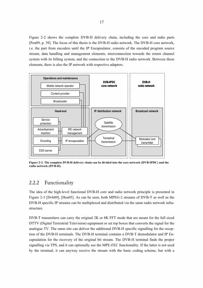
17

Figure 2-2 shows the complete DVB-H delivery chain, including the core and radio parts [Pen09, p. 39]. The focus of this thesis is the DVB-H radio network. The DVB-H core network, i.e. the part from encoders until the IP Encapsulator, consists of the encoded program source stream, data handling and management elements, interconnection towards the return channel system with its billing system, and the connection to the DVB-H radio network. Between these elements, there is also the IP network with respective adapters.

Service protection

Head-end

Advertisement insertion

Encoding

ESG server

IPE network management

IP encapsulation

Content provider

Broadcaster

Mobile network operator

IP distribution network Broadcast network

DVB-IPDCcore network

Operations and maintenanceDVB-H

radio network

Satellite transmission

Modulator and transmitter

Terrestrial transmission

Service protection

Head-end

Advertisement insertion

Encoding

ESG server

IPE network management

IP encapsulation

Content provider

Broadcaster

Mobile network operator

IP distribution network Broadcast network

DVB-IPDCcore network

Operations and maintenanceDVB-H

radio network

Satellite transmission

Modulator and transmitter

Terrestrial transmission

Figure 2-2. The complete DVB-H delivery chain can be divided into the core network (DVB-IPDC) and the radio network (DVB-H).

2.2.2 Functionality

The idea of the high-level functional DVB-H core and radio network principle is presented in Figure 2-3 [Dvb09], [Hen05]. As can be seen, both MPEG-2 streams of DVB-T as well as the DVB-H specific IP streams can be multiplexed and distributed via the same radio network infra-structure.

DVB-T transmitters can carry the original 2K or 8K FFT mode that are meant for the full sized DTTV (Digital Terrestrial Television) equipment or set top boxes that converts the signal for the analogue TV. The same site can deliver the additional DVB-H specific signalling for the recep-tion of the DVB-H terminals. The DVB-H terminal contains a DVB-T demodulator and IP En-capsulation for the recovery of the original bit stream. The DVB-H terminal finds the proper signalling via TPS, and it can optionally use the MPE-FEC functionality. If the latter is not used by the terminal, it can anyway receive the stream with the basic coding scheme, but with a

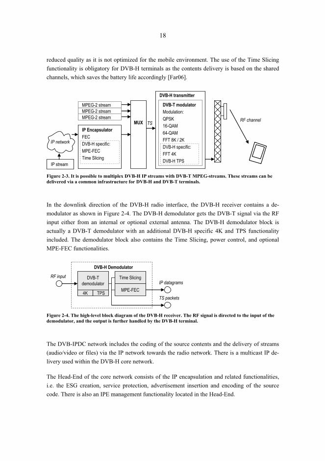
18

reduced quality as it is not optimized for the mobile environment. The use of the Time Slicing functionality is obligatory for DVB-H terminals as the contents delivery is based on the shared channels, which saves the battery life accordingly [Far06].

DVB-T modulatorModulation:QPSK16-QAM64-QAMFFT 8K / 2KDVB-H specific:FFT 4KDVB-H TPS

MUXIP EncapsulatorFECDVB-H specific:MPE-FECTime Slicing

MPEG-2 streamMPEG-2 streamMPEG-2 stream

DVB-H transmitter

RF channelTS

IP network

IP stream

Figure 2-3. It is possible to multiplex DVB-H IP streams with DVB-T MPEG-streams. These streams can be delivered via a common infrastructure for DVB-H and DVB-T terminals.

In the downlink direction of the DVB-H radio interface, the DVB-H receiver contains a de-modulator as shown in Figure 2-4. The DVB-H demodulator gets the DVB-T signal via the RF input either from an internal or optional external antenna. The DVB-H demodulator block is actually a DVB-T demodulator with an additional DVB-H specific 4K and TPS functionality included. The demodulator block also contains the Time Slicing, power control, and optional MPE-FEC functionalities.

DVB-Tdemodulator

MPE-FEC

Time Slicing

4K TPS

DVB-H Demodulator

RF inputIP datagrams

TS packets

Figure 2-4. The high-level block diagram of the DVB-H receiver. The RF signal is directed to the input of the demodulator, and the output is further handled by the DVB-H terminal.

The DVB-IPDC network includes the coding of the source contents and the delivery of streams (audio/video or files) via the IP network towards the radio network. There is a multicast IP de-livery used within the DVB-H core network.

The Head-End of the core network consists of the IP encapsulation and related functionalities, i.e. the ESG creation, service protection, advertisement insertion and encoding of the source code. There is also an IPE management functionality located in the Head-End.

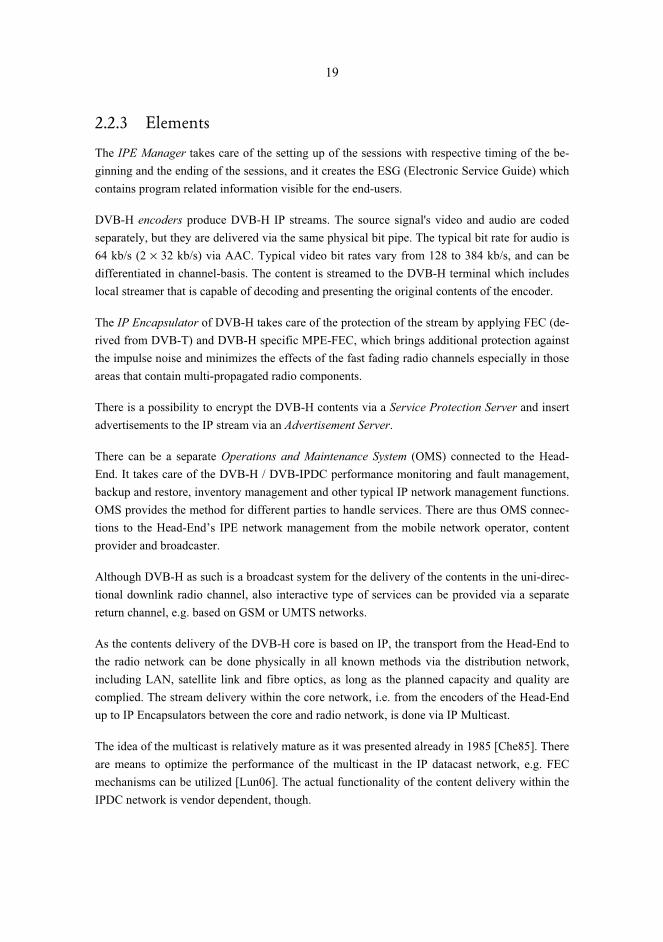
19

2.2.3 Elements

The IPE Manager takes care of the setting up of the sessions with respective timing of the be-ginning and the ending of the sessions, and it creates the ESG (Electronic Service Guide) which contains program related information visible for the end-users.

DVB-H encoders produce DVB-H IP streams. The source signal's video and audio are coded separately, but they are delivered via the same physical bit pipe. The typical bit rate for audio is 64 kb/s (2 × 32 kb/s) via AAC. Typical video bit rates vary from 128 to 384 kb/s, and can be differentiated in channel-basis. The content is streamed to the DVB-H terminal which includes local streamer that is capable of decoding and presenting the original contents of the encoder.

The IP Encapsulator of DVB-H takes care of the protection of the stream by applying FEC (de-rived from DVB-T) and DVB-H specific MPE-FEC, which brings additional protection against the impulse noise and minimizes the effects of the fast fading radio channels especially in those areas that contain multi-propagated radio components.

There is a possibility to encrypt the DVB-H contents via a Service Protection Server and insert advertisements to the IP stream via an Advertisement Server.

There can be a separate Operations and Maintenance System (OMS) connected to the Head-End. It takes care of the DVB-H / DVB-IPDC performance monitoring and fault management, backup and restore, inventory management and other typical IP network management functions. OMS provides the method for different parties to handle services. There are thus OMS connec-tions to the Head-End’s IPE network management from the mobile network operator, content provider and broadcaster.

Although DVB-H as such is a broadcast system for the delivery of the contents in the uni-direc-tional downlink radio channel, also interactive type of services can be provided via a separate return channel, e.g. based on GSM or UMTS networks.

As the contents delivery of the DVB-H core is based on IP, the transport from the Head-End to the radio network can be done physically in all known methods via the distribution network, including LAN, satellite link and fibre optics, as long as the planned capacity and quality are complied. The stream delivery within the core network, i.e. from the encoders of the Head-End up to IP Encapsulators between the core and radio network, is done via IP Multicast.

The idea of the multicast is relatively mature as it was presented already in 1985 [Che85]. There are means to optimize the performance of the multicast in the IP datacast network, e.g. FEC mechanisms can be utilized [Lun06]. The actual functionality of the content delivery within the IPDC network is vendor dependent, though.

20

2.3 Radio functionality

The audio / video stream or data file is delivered from the DVB-IPDC network to the DVB-H radio network, the IP Encapsulator being their interface. The signal is delivered to the DVB-H modulator, DVB-H transmitter and finally to the radio interface via the antenna system.

2.3.1 Radio transmitter

A typical DVB-H transmitter output power is in range of some hundreds of watts up to some thousands of watts. For the DVB-H radio transmission, the transmitter includes DVB-H specific functionality, although also separate DVB-H modulator can be used with the standard DVB-T transmitter. The DVB-H modulator can also be connected in front of an analogue transmitter if the power amplifier functions in the desired frequency and bandwidth.

Due to the physical obstacles like buildings and variations of the terrain height, outages can oc-cur in the coverage area of the site cell. The coverage of these problematic areas can be en-hanced by installing separate gap-fillers nearby, which are either passive or active repeaters. The latter can be either direct amplifier or regenerating one, which decodes, amplifies and codes again the bit stream. The output power of gap-fillers varies typically from few watts to some hundreds of watts. Gap-fillers may also perform a frequency translation. In practice, this variant is not useful in typical DVB-H networks as multiple channels are not likely to be available in reduced areas.

Even if gap-fillers could be used relatively freely to fill in the coverage holes, the location of these elements should be taken into account in the network planning in order to maximize the isolation between the receiving and transmitting end and thus to avoid the uncontrolled oscilla-tion effect which would lower the gain significantly [Gom09, p. 81].

2.3.2 Terminal

Figure 2-5 shows a high-level block diagram of the DVB-H receiver [Dvb09]. The reception of the Transport Stream (TS) in DVB-H is compatible with the DVB-T system, and the demodula-tion is thus done with same principles. The additional DVB-H specific functionality consists of the Time Sliced burst handling, the MPE-FEC module and the DVB-H de-encapsulation.

As can be seen from Figure 2-5, the FER information, i.e. frame errors before MPE-FEC func-tionality, is obtained after the Time Slicing process, and the MFER (remaining FER after MPE-FEC) is obtained after the MPE-FEC module. The IP level information is obtained after the de-modulation procedure.

21

DVB-H specificfunctionality

IP output

DVB-TDemodulator

DVB-HTime Slicing

DVB-HMPE-FEC

DVB-HDe-encapsulation

FER reference

MFER reference

IP reference

TS reference

RF reference

Figure 2-5. The DVB-H reference receiver.

The measurement point for the received RF power level is found after the antenna element and the optional GSM interference filter. There might also be an optional external antenna connector implemented in the terminal before the RF reference point. The presence of the filter and an-tenna connector has thus a frequency-dependent loss effect on the measured received power level in the RF point. It should be noted that the receiver antenna diversity can enhance the per-formance of DVB-H lowering the required C/N value with several dB [Far01, p. 11].

2.3.3 Frequency

DVB-H specifications define the system for VHF III (174�230 MHz), UHF IV (470�598 MHz) and UHF V (598�862 MHz) bands. There is also a possibility to adopt DVB-H to other fre-quencies like in L-band. As an example, DVB-H has been tested in USA in the 1.6 GHz band. In practice, the terminal’s DVB-H engine might contain a limited band, e.g. 470�702 MHz as stated in [Nok05] because the upper frequencies of UHF are close to the GSM 850 system which might cause interferences to the reception of DVB-H. On the other hand, despite the good propagation characteristics, the lowest frequencies in the VHF band are demanding for the re-ceiver’s physical antenna dimensions as the wavelength is relatively large [Far05]. In Europe, the UHF is identified as the primary band for DVB-H [Bmc07b, p.3].

According to the specifications, the DVB-H frequency bandwidth can be 6, 7 or 8 MHz. There is also an additional bandwidth of 5 MHz included to the specification. These bandwidth values of DVB-H correspond to the analogue TV channel division in different countries. The modula-tion bandwidth of DVB-H is mapped into these frequency bandwidth values in such a way that it is the difference between the last (N) and the first carrier of the OFDM symbol being equal to

22

(N-1)/TS, where TS is the symbol length. This results in a modulation bandwidth of 4.76 MHz, 5.71 MHz, 6.66 MHz and 7.61 MHz, respectively, for the bands of 5, 6, 7 and 8 MHz.

Figure 2-6 shows the frame structure of DVB-H. The symbol forms the basic unit which has duration of TS. There are 68 symbols in a single frame which has duration of TF. The frames are repeated in superframe cycles.

TUTGI

Symbol (duration: TS)

670 1 2 3 66...

1 2 3 4

Frame (duration: TF)

Guard Interval

Useful symbol

Figure 2-6. The frame structure of DVB-H.

The DVB-H symbol consists of the Guard Interval (GI) and the useful part that delivers the data. GI is needed in order to cope with the multipath propagation with a delay spread less than the GI determinates. The useful part contains the OFDM carriers of f1…fN. The carrier spacing is 1/TU for the separation of two consecutive carriers. The channel bandwidth Bch = (fN–f1) is thus (N–1)/TU. The amount of carriers (that are transferring pilot and data information) within a single symbol depends on the FFT mode. In the 2K mode, the carrier number is 1705, in the 4K mode 3409, and in the 8K mode it is 6817. A total of 68 consecutive symbols (numbered from 0 to 67) form a superframe which is repeated in cycles [Sci07].

2.3.4 OFDM parameters

DVB-H is based on OFDM (Orthogonal Frequency Division Multiplexing). It is a spread spec-trum technique that delivers the high speed bit stream via several subcarriers each containing lower speed bit streams. It is used in various systems like DVB-T, LTE, ADSL and WiMAX. The transmission of OFDM subcarriers is parallel, and they are separated by different frequen-cies as shown in Figure 2-7 [Far07]. The information is distributed in an interleaved way to the multiple subcarriers with the error protection, resulting COFDM (Coded Orthogonal Frequency Division Multiplexing) [Fis08, p. 316], [Wan03, p. 952].

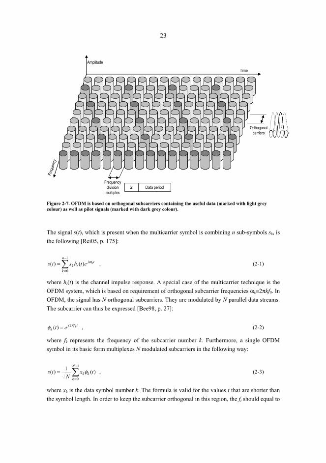
23

Time

Freq

uenc

y

Frequency division

multiplex

Orthogonal carriers

GI Data period

Amplitude

Figure 2-7. OFDM is based on orthogonal subcarriers containing the useful data (marked with light grey colour) as well as pilot signals (marked with dark grey colour).

The signal s(t), which is present when the multicarrier symbol is combining n sub-symbols sk, is the following [Rei05, p. 175]:

�−

=

=1

0

)()(n

k

tjtk

kethsts ω , (2-1)

where ht(t) is the channel impulse response. A special case of the multicarrier technique is the OFDM system, which is based on requirement of orthogonal subcarrier frequencies ωk≡2πkf0. In OFDM, the signal has N orthogonal subcarriers. They are modulated by N parallel data streams. The subcarrier can thus be expressed [Bee98, p. 27]:

tfjk

ket πφ 2)( = , (2-2)

where fk represents the frequency of the subcarrier number k. Furthermore, a single OFDM symbol in its basic form multiplexes N modulated subcarriers in the following way:

�−

=

=1

0

)(1)(N

kkk tx

Nts φ , (2-3)

where xk is the data symbol number k. The formula is valid for the values t that are shorter than the symbol length. In order to keep the subcarrier orthogonal in this region, the ft should equal to

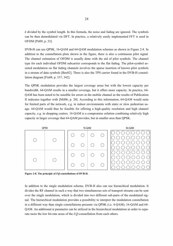
24

k divided by the symbol length. In this formula, the noise and fading are ignored. The symbols can be then demodulated via DFT. In practice, a relatively easily implemented FFT is used in OFDM [Pit09, p. 33].

DVB-H can use QPSK, 16-QAM and 64-QAM modulation schemes as shown in Figure 2-8. In addition to the constellation plots shown in the figure, there is also a continuous pilot signal. The channel estimation of OFDM is usually done with the aid of pilot symbols. The channel type for each individual OFDM subcarrier corresponds to the flat fading. The pilot-symbol as-sisted modulation on flat fading channels involves the sparse insertion of known pilot symbols in a stream of data symbols [Bee02]. There is also the TPS carrier found in the DVB-H constel-lation diagram [Fis08, p. 337, 342].

The QPSK modulation provides the largest coverage areas but with the lowest capacity per bandwidth. 64-QAM results in a smaller coverage, but it offers more capacity. In practice, 64-QAM has been noted to be sensible for errors in the mobile channel as the results of Publication II indicates together with [Mil06, p. 20]. According to this information, 64-QAM would suite for limited parts of the network, e.g. in indoor environments with static or slow pedestrian us-age. 64-QAM would thus be feasible for offering a high-quality resolution and high channel capacity, e.g. in shopping centres. 16-QAM is a compromise solution combining relatively high capacity in larger coverage that 64-QAM provides, but in smaller area than QPSK.

QPSK 16-QAM 64-QAM

Figure 2-8. The principle of I/Q constellations of DVB-H.

In addition to the single modulation scheme, DVB-H also can use hierarchical modulation. It divides the RF channel in such a way that two simultaneous sets of transport streams can be sent over the single modulation, which is divided into two different sub-parts of the modulated sig-nal. The hierarchical modulation provides a possibility to interpret the modulation constellation in a different way than single constellations presents via QPSK (i.e. 4-QAM), 16-QAM and 64-QAM. An additional α parameter can be utilized in the hierarchical modulation in order to sepa-rate more the low bit-rate areas of the I/Q-constellation from each others.

25

One of the essential OFDM parameters for DVB-H is the FFT size that represents the amount of modulated subcarriers. In DVB-H, it can be the original DVB-T value of 2K or 8K, as well as the DVB-H specific 4K. The 4K size is a compromise which results in a balanced performance between the terminal speed and the SFN size. 8K provides with largest SFN areas (without in-terferences) but with the cost of the maximum terminal speed. 2K offers reversed benefits, i.e. highest terminal speeds but with the cost of reduced SFN size.

Guard Interval (GI) is also a relevant parameter for DVB-H. It can have values of 1/4, 1/8, 1/16 and 1/32, each representing the proportion of the signal that is not used for the delivery of the data. GI affects directly on the SFN size. GI is important in order to reduce negative effects of the multipath radio propagation, including those paths caused by the environment itself (e.g. buildings) as well as co-channel interferences in case of the SFN network.

The combination of FFT and GI parameter values determines the maximum distance between physical DVB-H transmitters [Dvb09], [Mil06] as shown in Table 2-1.

Table 2-1. The effect of the GI and FFT size as a function of the maximum tolerable signal delay and the longest non-interfering distance between transmitters within SFN.

Guard interval time / maximum SFN diameter FFT mode

GI=1/4 GI=1/8 GI=1/16 GI=1/32

FFT=2K 56 μs / 16.8 km 28 μs / 8.4 km 14 μs / 4.2 km 7 μs / 2.1 km

FFT=4K 112 μs / 33.6 km 56 μs / 16. 8 km 28 μs / 8.4 km 14 μs / 4.2 km

FFT=8K 224 μs / 67.2 km 112 μs / 33.6 km 56 μs / 16.8 km 28 μs / 8.4km

As can be seen, longer guard interval means higher immunity to inter-OFDM symbol interfer-ences. In practice, longest GI values do have most significant benefits in static channel types like AWGN-channel [Mil06]. According to simulations and practical field tests [Mil06], shorter GI values do have better Doppler tolerance compared to longer ones. According to [Mil06], the maximum Doppler performance enhances linearly about 25% when {GI=1/4} is changed to {GI=1/32}.

2.3.5 Error recovery

Error control coding is an essential part of mobile communication systems. The error detection and recovery of DVB-H is based on the inner forward error correction (FEC) that is also used in DVB-T. As the receiving end can recover the occurred errors up to a certain parameter depend-ent limit, it is especially suitable for uni-directional broadcast systems like DVB. Both DVB-H and DVB-T defines five levels for the respective code rate (CR), i.e. 1/2, 2/3, 3/4, 5/6 and 7/8. There is also an optional in-depth interleaver defined for DVB-H. It can be used to increase the robustness of 2K and 4K modes as they can be used to further widen the depth of the native 8K

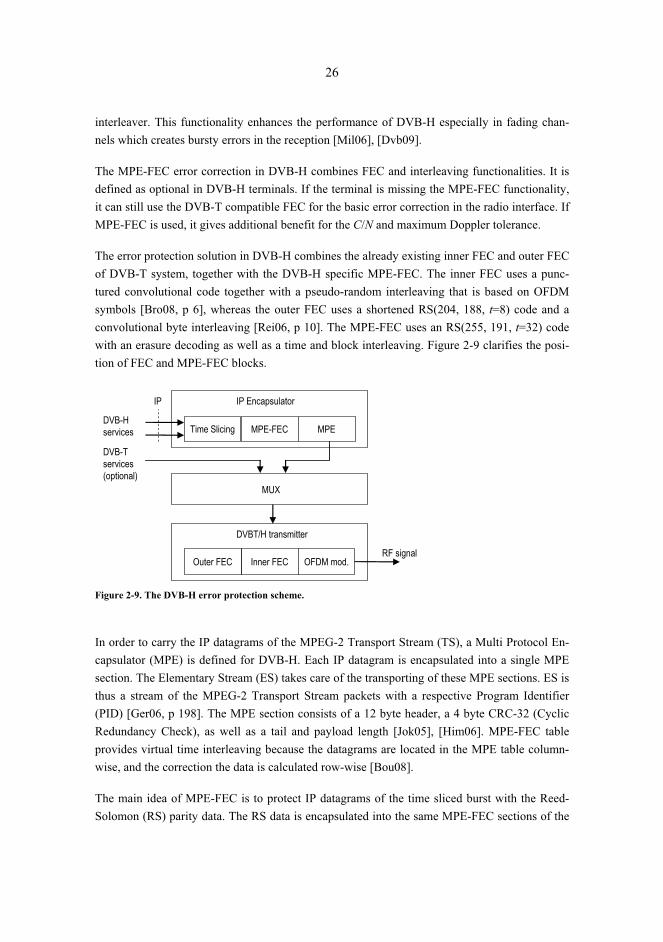
26

interleaver. This functionality enhances the performance of DVB-H especially in fading chan-nels which creates bursty errors in the reception [Mil06], [Dvb09].

The MPE-FEC error correction in DVB-H combines FEC and interleaving functionalities. It is defined as optional in DVB-H terminals. If the terminal is missing the MPE-FEC functionality, it can still use the DVB-T compatible FEC for the basic error correction in the radio interface. If MPE-FEC is used, it gives additional benefit for the C/N and maximum Doppler tolerance.

The error protection solution in DVB-H combines the already existing inner FEC and outer FEC of DVB-T system, together with the DVB-H specific MPE-FEC. The inner FEC uses a punc-tured convolutional code together with a pseudo-random interleaving that is based on OFDM symbols [Bro08, p 6], whereas the outer FEC uses a shortened RS(204, 188, t=8) code and a convolutional byte interleaving [Rei06, p 10]. The MPE-FEC uses an RS(255, 191, t=32) code with an erasure decoding as well as a time and block interleaving. Figure 2-9 clarifies the posi-tion of FEC and MPE-FEC blocks.

Time Slicing MPE-FEC MPE

IP Encapsulator

DVB-H services

IP

MUX

DVB-T services(optional)

DVBT/H transmitter

Outer FEC Inner FEC OFDM mod.RF signal

Figure 2-9. The DVB-H error protection scheme.

In order to carry the IP datagrams of the MPEG-2 Transport Stream (TS), a Multi Protocol En-capsulator (MPE) is defined for DVB-H. Each IP datagram is encapsulated into a single MPE section. The Elementary Stream (ES) takes care of the transporting of these MPE sections. ES is thus a stream of the MPEG-2 Transport Stream packets with a respective Program Identifier (PID) [Ger06, p 198]. The MPE section consists of a 12 byte header, a 4 byte CRC-32 (Cyclic Redundancy Check), as well as a tail and payload length [Jok05], [Him06]. MPE-FEC table provides virtual time interleaving because the datagrams are located in the MPE table column-wise, and the correction the data is calculated row-wise [Bou08].

The main idea of MPE-FEC is to protect IP datagrams of the time sliced burst with the Reed-Solomon (RS) parity data. The RS data is encapsulated into the same MPE-FEC sections of the

27

burst with the actual data. The RS part of the burst belongs to the same elementary stream (MPE section), but they have different table identifications. The benefit of this solution is that the re-ceiver can distinguish between sections, and if the terminal does not have the capability to use the DVB-H specific FEC, it can decode in any case bursts although with lower error correction quality when the terminal experiences difficult radio conditions.

The part of the MPE-FEC frame that includes IP datagrams is called Application Data Table (ADT). ADT has a total of 191 columns. In case IP datagrams do not fill completely the ADT field, the remaining part is padded with zeros. The division between ADT and RS table is shown in Figure 2-10. The number of RS rows can be selected from 256, 512, 768 and 1024. The amount of rows is indicated in Service Information (SI). The RS data has a total of 64 columns. For each row, 191 IP datagram bytes are used for calculating 64 parity bytes of RS rows. Also in this case, if the row is not filled completely, padding is applied. The result is a relative deep interleaving as the application data is distributed over the whole burst.

.

.

.

.

.

.

IPdatagrams

PADDED

SPACE

PADDED

SPACE

PADDED

SPACE

.

.

.

1st byte

2nd byte PUNCTURED

COLUMNS

RSparity bytes

191 data columns 64 RS columns

256,512,768or

1024rows

. . .

. . .

Figure 2-10. The MPE-FEC frame consists of the application data table for IP datagrams and the RS data table for RS parity bytes.

The Reed-Solomon code is based on the polynomial correction method. The polynomial is en-coded for the transmission over the air interface. If the data is corrupted during the transmission, the receiving end can calculate the expected values of the data within a certain setting specific limit.

The RS data of DVB-H is sent in encoded blocks, with a total number of m-bit symbols in the encoded block of n = 2m – 1 [Pos05, p. 22]. With 8-bit symbols the amount of symbols per block is n = 28 – 1 = 255. This is thus the total size of the DVB-H frame. The actual user data inside

28

the frame is defined as a parameter value k, which indicates the number of data symbols per block. The normal value of k is 223 and the number of parity symbols is 32 (with 8 bits per symbol). The universal format of presenting these values is (n, k) = (255, 223). In this case, the code is capable of correcting up to 16 symbol errors per block. RS can correct the errors de-pending on the redundancy of the block. For the erroneous symbols whose location is not known in advance, the RS code is capable of correcting up to (n–k)/2 symbols. This means that RS can correct half as many errors as the amount of redundancy symbols is added to the block.

If the location of errors is known (indicating erasures), then RS can correct twice as many erasures as errors. If E is the number of errors and S is the number of erasures in the block, the error correction capability is given by 2E+S < n.

The characteristic of RS error correction is well suited to the environment with a high probabil-ity of errors occurring in bursts, like happens typically in the radio interface. This is because it does not matter how many bits are erroneous in the symbol. If multiple errors occur in byte, it is considered as a one single error. It is possible to use also other block sizes. The shortening can be done by padding the remaining (empty) part of the block (bytes). These padded bytes are not transmitted, but the receiving end fills in automatically the empty space.

FEC consists of block and convolutional coding parts. RS is an example of the block coding, where blocks or packets of bits (symbols) are of a fixed size whereas the convolutional coding is based on bit or symbol lengths. In practice, block and convolutional codes are combined in con-catenated coding schemes; the convolutional coding handles the major part of the process whilst the block code, e.g. RS, carries out the recovery of the remaining errors as much as possible af-ter the convolutional coding. In mobile communications, convolutional codes are mostly de-coded with the Viterbi algorithm. The Viterbi algorithm is an error-correction scheme for noisy digital communication links. It is widely used, e.g. in GSM, dial-up modems, satellite commu-nications and in 802.11 LANs.

The performance of different RS decoding schemes has been investigated in [Jok05] and [Him06]. The MPE-FEC error detection and correction can be done based on conventional non-erasure RS decoding, where a maximum of 32 erroneous RS symbols, or bytes, are allowed on each row of the MPE-FEC frame. Frames of one or more rows with more than 32 errors are in-terpreted as erroneous. Another option for the MPE-FEC is to use erasure decoding, as has been selected for the DVB-H. In that case, a complete section is marked as unreliable if it contains an error. One section erasure leads to one column erasure in the MPE-FEC frame, when the IP datagram length equals to the number of rows in the MPE-FEC frame. For the erasure decoding a maximum of 64 erasures are allowed on a single row in the MPE-FEC frame. Frames con-sisting of at least one row with more than 64 erasures are considered erroneous. The perform-ance of different decoding schemes depends on the radio channel type, the AWGN channel in open areas being more controlled than the multipath channel of city centres. Simulation results

29

of [Jok05] show that the non-erasure decoding is substantially stronger in the AWGN environ-ment than in multipath cases. The performance of the non-erasure decoding is furthermore bet-ter in bursty error cases if the error distribution is uniform.

The transmitted data contains a checksum, which is typically created via CRC-32, but the stan-dard leaves the selection of the terminal’s decoding method for receiver designers. The use of CRC-32 in the receiver is thus optional. A probable reason for the selection of the erasure de-coding in DVB-H has been the need to reduce the computational complexity of conventional Reed-Solomon decoding algorithms, even if the over-head due to CRC-32 increases regardless of it’s use in the terminal’s side.

It is shown in [Him06] that decoding methods inserting also erroneous data into the MPE-FEC frame are in fact more efficient than erasure decoding methods suggested in the DVB-H stan-dard. The gain seem to exceed 1 dB in favour of so called hierarchical transport stream decod-ing if compared to the pure section erasure decoding. Results of [Him06] indicate that the end-user’s video quality can be increased significantly when allowing erroneous data to be used for decoding and passed to the application layer rather than using erasure decoding methods, where erroneous IP packets or even MPE-FEC frames are rejected.

Furthermore, [Jok06] claims that all other investigated decoding methods including the TSE decoding (transport stream erasure derived from the transport stream headers) that ignore the CRC-32 information would perform better than the CRC Erasure decoding. These findings indi-cate that the optimal setting for the decoding method can improve significantly the subjective DVB-H reception quality level that the end-user experiences.

2.3.6 Time Slicing

The basic idea of the Time Slicing functionality is to send the DVB-H specific elementary stream data in bursts with a higher data rate than the actual average bit rate of the stream would be. This allows the terminal to get a certain data stream portion in advance and to switch off the receiver whilst the terminal buffers the data and presents the video and/or audio content. The obvious advantage of the functionality is the battery saving as the power consumption of the receiver gets considerably lower. According to [Far06], the normal power saving is typically in order of 90�95 %. The significance of the final power saving of the terminal lowers, though, as there are applications and functionalities, e.g. the video streamer and the mobile system trans-ceiver which consumes their proportion of the processing power.

The Time Slicing functionality also provides the possibility to perform a seamless handover between the frequencies, because the terminal can monitor other MFN's during the off-period of the reception.

30

Figure 2-11 shows the principle of the Time Slicing functionality. The burst window can consist of several time sliced bursts, but the terminal needs to activate itself only when the contents of the own channel is transmitted.

The correct dimensioning of the Time Slicing functionality is important as it affects directly on the waiting period when the user changes the time sliced channel. The interval of the time sliced burst can be calculated when the peak bit rate, the average ES bit rate and the complete burst size are known. Assuming the average bit rate is 500 kb/s, the peak bit rate is 10 Mb/s, and the burst size is 2 Mb, the burst cycle is 4 seconds. In this case, it can be estimated that the average waiting time of the switching that the user experiences is approximately 2 seconds (an average of the extreme values). Taking the typical DVB-T channel switching time as a reference, it can be estimated that the channel switching time of less than 2 seconds is still tolerable from the user’s point of view.

Averagebit rate

Time (s)

BurstRate(kb/s)

Peak bit rate of single burst

On Off

Windowfor thebursts

Single frame

Figure 2-11. The principle of the Time Slicing functionality.

The header of each MPE section contains a delta-t parameter. It indicates the time for the be-ginning of the next time sliced burst. In this way, it is not necessary to synchronize the receiver and transmitter separately as the timing for the next reception is indicated in each burst.

2.3.7 SFN / MFN

DVB-H can be deployed as a single frequency network (SFN) or multi frequency network (MFN). In practice, the network may consist of both modes. One of the feasible strategies is to cover single cities with SFN isles, and the remaining part of the network can be done as MFN in order to inter-connect the isles.

When the DVB-H terminal moves from the coverage area of one DVB-H cell to another, the Time Slicing functionality provides a fluent frequency handover in the MFN mode. This is a re-sult of the off-time period of the time sliced bursts, as the terminal can scan the other frequen-

31

cies during this time. The terminal evaluates the best frequency, and when the order change, the terminal executes the handover process during the off-time period. The scanning procedure is implementation dependent as stated in [Dvb07], which also describes various use cases for the handover.

Time Slicing provides a seamless MFN-handover without disturbing the fluent following of the received contents. The handover process requires though a sufficiently good overlapping of the cell coverage areas. In case the same content is delivered via different adjacent cells, the syn-chronization of the site transmitters is important. This provides a transparent delivery of the contents to the users.

SFN provides the fluent implementation of the transmitters inside the theoretical limits of the SFN network area. New transmitters can be added to the same frequency basically without extra planning efforts whenever the SFN limits are not exceeded and the correct setting of the trans-mitter synchronization is taken care of, by default via the GPS timing. In this case, the overlap-ping parts of the coverage provide additional SFN gain.

The functionality and the gain due to the combination of separate signals, e.g. echoes from the individual transmitter as well as signals from separate transmitters, is based on the sum of all the received multipath components [Rei05, p. 178]. If the separate components are within the win-dow determined by the guard interval, the summing of the paths can be done without affecting interferences as shown in Figure 2-12.

TGI TU

First OFDM symbol

First OFDM symbol

First OFDM symbol

GI

GI

GI

Second OFDM symbol

Second OFDM symbol

Second OFDM symbol

Second OFDM symbolFirst OFDM symbol

Interference

1st path:

2nd path:

3rd path:

Sum of paths:

TGI TU

First OFDM symbol

First OFDM symbol

First OFDM symbol

GI

GI

GI

Second OFDM symbol

Second OFDM symbol

Second OFDM symbol

Second OFDM symbolFirst OFDM symbol

Interference

1st path:

2nd path:

3rd path:

Sum of paths:

Figure 2-12. The summing of the separate multi-path components can be done in the useful time window TU whilst all the components occur within the time delay TGI determined by the guard interval.

The COFDM bit stream is distributed over several individual carriers, i.e. the transmission is carried out by spreading the baseband bit stream. A set of carriers form a COFDM symbol. The processing of symbols is parallel. Before the receiver starts to evaluate the individual symbol, it waits a time window determined by TGI, i.e. during the guard interval in order to collect all the echoes. When the echoes occur within the GI window, they can be combined in order to add

32

energy for the original signal [Rei98, p. 4]. This enhances the carrier to noise and interference ratio of the received signal, resulting in a gain in the cell coverage and/or capacity. In practice, part of the symbol is copied from the beginning of the symbol to the end, which increases its duration determined by the guard interval [Gre06, p. 26].

The evaluation of the symbol takes place inside the FFT window determined by TU, and the or-thogonal criterion is also considered within this original symbol duration, without considering the extended part of the signal. The FFT window position is then selected depending on the re-ceived radio components.

If the SFN limits are exceeded, i.e., there are sites outside of the theoretical SFN area, they start acting as interfering sources in those locations where the radio propagation delay is higher than the GI determines. Whilst the level of the combined useful carrier is high enough compared to the total interference level, as Publications III, IV, VII and X show, the exceeding of the SFN limits can be done in a controlled way, and it is possible to find optimal parameter sets by bal-ancing the SFN gain and SFN interferences. The assumption of the above mentioned publica-tions is that the total contribution of interfering components, as well as the useful carrier com-ponents, can be calculated by summing directly the power levels of separate radio components that are propagated form different sites.

In the investigations of this thesis, the minimum required C/(N+I) ratio as presented in [Dvb09, p96] was utilized as criteria. The value depends on the channel type, and the minimum value is also frequency selective over the considered bandwidth. Nevertheless, as this higher-level value set includes effects of the channel type, the respective behaviour of the C/N and C/(N+I) was not investigated in more detailed level in Publications of this thesis.

2.3.8 Interaction channel

The DVB-H system does not define the uplink communications for the interactions. Neverthe-less, the uplink part can be included via the other delivery mechanisms, e.g. by using GSM or UMTS networks. The management of the chargeable channels can also be done by using the local terminal functionality. One possibility for the DVB-H stand-alone terminal can be based on separate codes that are delivered in form of scratch cards.

The interaction channel provides means for the opening of the ciphered contents, and it can be used, e.g. for the real time voting type of activities during a television program. In theory, there are no obstacles in using any other radio interfaces for the interactions, like WLAN. In any case, the most logical combination is the DVB-H and GSM/UMTS modules integrated physically into the same terminal, as the coverage areas of the 2G and 3G mobile networks can be assumed to usually overlap with DVB-H.

33

In a typical DVB-H network planning process, it can be assumed that DVB-H and GSM/UMTS networks are overlapping. The overlapping is most perfect if DVB-H can be co-sited with mo-bile communication networks.

As suggested in [Ung06], in order to build a DVB-H network, position and size of site cells could be selected to maximize the benefit of a hybrid network. The implementation of the DVB-H network on top of the existing 3G and DVB-T network infrastructure is attractive also be-cause it lowers the initial network investments [Had07]. Furthermore, as suggested in [Gom07], the DVB-H and mobile communications networks could collaborate more in such a way that the DVB-H deployment is incremental, mobile networks providing seamlessly a secondary route.

Despite the obvious benefits of the collaborating mode, the challenge in the hybrid network is the establishment of the in-depth co-operation between different infrastructure owners. When data is sent over separate networks, the additional challenge arises from the practical fact that the common algorithms and data flow management methods are not straightforward to deploy for different live networks. Also the site reuse for DVB-H and other systems is not necessarily easy in practice due to the potential non-technical restrictions. For this reason, the analyses of this thesis are based on the assumption of the stand-alone DVB-H network.

Nevertheless, in practice, there might be locations where the coverage areas of either DVB-H or mobile communications networks are present as shown in Figure 2-13. In these cases, the interaction channel does not work at that specific moment and/or location, and it is thus impos-sible to initiate the opening procedure of a channel that requires separate signalling in order to be used. If the initiation has been done earlier, the channel can be used without the presence of an interaction channel until the possible expiration time of the channel deciphering and scram-bling key validity is reached.

DVB-H coverage

GSM/UMTS coverage

DVB-H coverage

GSM/UMTS coverage

Figure 2-13. The principle of overlapping GSM/UMTS coverage areas.

In case of the in-depth radio analysis, if the DVB-H interaction is utilized via 2G/3G, it might be interesting to take into account the effects of the packet switched data on the mobile network

34

performance. As concluded in [Pen99], [Pen99b] and [Pir99], the amount of the GSM traffic load can have an effect on the useful coverage areas, because the varying load might create a small-scale UMTS-type of cell breathing in the cell edge areas of the network’s non-BCCH fre-quencies, i.e., in the frequency hopping layer of GSM.

In practice, though, the C/I of typical GSM mobile networks is dimensioned into a sufficiently high level which provides enough overlapping areas even in the presence of co-channel interfer-ences, which thus minimizes the presence of the outages within the planned coverage areas. Also UMTS can be assumed to provide a sufficiently robust performance even in the highest load cases. For this reason, the investigation of the effect of the 2G/3G traffic load on the suc-cess rate can be rejected in those cases of the interactions where the common DVB-H and mo-bile communications networks are found.

35

3 Initial radio network planning

process

3.1 High-level network dimensioning process

The dimensioning of the high level DVB-H radio network can be summarized by presenting three main variables, i.e. the channel capacity, the coverage area and the quality of the service, which all together have effect on the total cost of the network as illustrated in Figure 3-1. The network with poor capacity, coverage and QoS (Quality of Service) has a minimum cost, but the revenue per customer would also be low due to the unsatisfactory service. On the other hand, the highly overlapping and high-capacity network with excellent outdoor and indoor coverage in a large area is technically desirable, but the cost for the building and operating of the network might be too high in order to recover the expenses as there is a practical limit for the user fees.

Cost

Capacity

Coverage QoS

Figure 3-1. The high-level cross-relations of the most relevant DVB-H radio network planning items.

The task is thus to design a network with sufficiently high quality, and with initial and operating costs that can be recovered in a planned time period, e.g. via monthly fees. It can be estimated that the quality of the network is on correct level when the customers are willing to use the ser-vice and accept the technical performance of the services as well as the related usage fee. In the complete network design, it is thus essential to take into account both technical issues as well as their costs, and to seek for their balance in order to make sure that the return of investments (ROI) are on acceptable level.

As an example of the cross-relation between the values, by keeping the site number the same, 16-QAM modulation would offer high-capacity with lower coverage, whilst QPSK offers less capacity but in larger area with the same location probability for the coverage.

36

A process chart shown in Figure 3-2 was created as a part of this thesis as a basis for the nomi-nal network planning in order to find the relevant items of the planning and optimisation of the DVB-H radio network in the initial phase. The presented process chart provides an approxima-tion of the number of needed sites by the utilisation of the uniform radio planning assumptions for all the sites.

In this initial planning phase, there is not yet need for a detailed analysis that take into account the realistic site locations and topological variations, different antenna heights and power levels. Nevertheless, the high-level regulatory limitations for the maximum power should be known.

Capacity planningInput: total capacity and/or number of channels with possibly requirement for

kb/s. Set the parameters: modulation, FFT, GI that complies with the requirement.

Output: set of parameter values that provides the channels.

Coverage planningInput: quality level (area location probability).

Apply link budget and prediction models, tune antenna height, transmitter power level (max: regulatory limit)Output: radius per cell (generic)

Is the coverage per site good enough?No Yes

Is it possible to tune the coverage related parameters?

Cost optimizationCalculate the total network cost

(CAPEX, OPEX per x year)

Acceptable level of costs vs. technical performance?No Yes

Go to detailed planning process

General nominal radio network assumptions

Is the EMC and radiation safety ok?No Yes

yes

noChange the capacity requirement

Change the coverage

parameter values and/or quality

level requirement.

Initial optionsSelect transmitter type (power levels), antenna types (gains), general

assumptions for the environment type (% of dense urban/urban/sub-urban, rural)

Change the transmitter type (maximum power levels), antenna

types (gains)

Figure 3-2. The proposed radio network planning process in the initial phase. The process contains high-level estimations of the capacity and coverage by taking into account the economical and regulatory limitations.

37

3.2 Capacity planning

In the initial phase of the DVB-H network planning, the procedure is to decide first the offered capacity of the system. The total capacity in certain DVB-H bandwidth ⎯ defined as 5, 6, 7, or 8 MHz ⎯ affects also on the size of the site coverage area. The dimensioning process is thus iterative, and the aim is to find a balance between the capacity, coverage and cost of the net-work.

The capacity can be varied by adjusting the modulation, guard interval, code rate and channel bandwidth. As an example, the parameter set of QPSK, GI 1/4, code rate 1/2 and channel band-width 8 MHz provides a total capacity of 4.98 Mb/s, which can be divided into one or more electronic service guides (ESG) and various audio/video sub-channels with about 200–500 kb/s bit stream dedicated for each.

The capacity does not depend on the number of carriers which is indicated by the FFT mode. Nevertheless, the selected FFT affects on the Doppler shift tolerance. As a comparison, the pa-rameter set of 16-QAM, GI 1/32, code rate 7/8 and channel bandwidth of 8 MHz, provides a total capacity of 21.1 Mb/s. It should be noted, though, that the latter parameter set is not practi-cal due to the clearly increased C/N requirement which reduces considerably the useful cover-age area and makes the reception sensible for the variations in the radio interface.

Table 3-1 shows the reachable capacity in Mbit/s per a total DVB-H frequency band as a func-tion of the radio parameter values. This useful bit rate would be reduced accordingly by the di-rect proportion of MPE-FEC rate when it is present, i.e. MPE-FEC rate of 3/4 (which corre-sponds about 25 % of overhead) results in 3/4 out of the original capacity value to be available for the useful bits. In this sense, e.g. the combination of CR of 1/2 and MPE-FEC of 1/2 results in the highest protection over the radio transmission but with the lowest capacity.

Table 3-1. The summary of total DVB-H bitrates as a function of the parameter values as presented in [Dvb09]. The values for the 5 MHz band can be extrapolated from the others.

GI=1/4 GI=1/8 GI=1/16 GI=1/32 Modul. CR 6MHz 7MHz 8MHz 6MHz 7MHz 8MHz 6MHz 7MHz 8MHz 6MHz 7MHz 8MHz 1/2 3.73 4.35 4.98 4.14 4.83 5.53 4.39 5.12 5.85 4.52 5.27 6.03 2/3 4.97 5.80 6.64 5.52 6.45 7.37 5.85 6.83 7.81 6.03 7.03 8.04 3/4 5.59 6.53 7.46 6.22 7.25 8.29 6.58 7.68 8.78 6.78 7.91 9.05 5/6 6.22 7.25 8.29 6.91 8.06 9.22 7.31 8.53 9.76 7.54 8.79 10.05

QPSK

7/8 6.53 7.62 8.71 7.25 8.46 9.68 7.68 8.96 10.25 7.91 9.23 10.56 1/2 7.46 8.70 9.95 8.29 9.67 11.06 8.78 10.24 11.71 9.04 10.55 12.06 2/3 9.95 11.61 13.27 11.05 12.90 14.75 11.70 13.66 15.61 12.06 14.07 16.09 3/4 11.19 13.06 14.93 12.44 14.51 16.59 13.17 15.36 17.56 13.57 15.83 18.10 5/6 12.44 14.51 16.59 13.82 16.12 18.43 14.63 17.07 19.52 15.08 17.59 20.11

16-QAM

7/8 13.06 15.24 17.42 14.51 16.93 19.35 15.36 17.93 20.49 15.83 18.47 21.11 1/2 11.19 13.06 14.93 12.44 14.51 16.59 13.17 15.36 17.56 13.57 15.83 18.10 2/3 14.92 17.41 19.91 16.58 19.35 22.12 17.56 20.49 23.42 18.09 21.11 24.13 3/4 16.79 19.59 22.39 18.66 21.77 24.88 19.76 23.05 26.35 20.35 23.75 27.14 5/6 18.66 21.77 24.88 20.73 24.19 27.65 21.95 25.61 29.27 22.62 26.39 30.16

64-QAM

7/8 19.59 22.86 26.13 21.77 25.40 29.03 23.05 26.89 30.74 23.75 27.71 31.67

38

The first task of the initial capacity planning is thus to select the whole parameter value set that complies with the target capacity value. As an example, if the target capacity value is a mini-mum of 8 Mb/s, and the bandwidth is 8 MHz, Table 3-1 indicates the compliant parameter val-ues for QPSK that are {GI=1/4, CR=5/6}, {GI=1/4, CR=7/8}, {GI=1/8, CR=3/4}, {GI=1/8, CR=5/6}, {GI=1/8, CR=7/8}, {GI=1/16, CR=3/4}, {GI=1/16, CR=5/6}, {GI=1/16, CR=7/8}, {GI=1/32, CR=2/3}, {GI=1/32, CR=3/4}, {GI=1/32, CR=5/6} and {GI=1/32, CR=7/8}. For the 16-QAM and 64-QAM modulations, all the GI and CR combinations complies with the mini-mum requirement of 8 Mb/s in this case.

Knowing that the MPE-FEC rate will reduce the final useful data with the direct proportion, the set of the compliant parameters is reduced in the following way when the MPE-FEC is added:

• For MPE-FEC 7/8: {QPSK, GI=1/8, (CR=5/6, 7/8)}, {QPSK, GI=1/16, (CR=5/6, 7/8)}, {QPSK, GI=1/32, (CR=5/6, 7/8)}, {16-QAM, GI=all, CR=all}, {64-QAM, GI=all, CR=all}

• For MPE-FEC 5/6: {QPSK, GI=1/8, CR=7/8}, {QPSK, GI=1/16, (CR=5/6, 7/8)}, {QPSK, GI=1/32, (CR=5/6, 7/8)}, {16-QAM, GI=all, CR=all}, {64-QAM, GI=all, CR=all}

• For MPE-FEC 3/4: {16-QAM, GI=1/4, (CR=2/3, 3/4, 5/6, 7/8)}, {16-QAM, (GI=1/8, 1/16, 1/32), CR=all}, {64-QAM, GI=all, CR=all}

• For MPE-FEC 2/3: {16-QAM, GI=1/4, (CR=2/3, 3/4, 5/6, 7/8)}, {16-QAM, GI=1/8, (CR=2/3, 3/4, 5/6, 7/8)},{16-QAM, GI=1/16, (CR=2/3, 3/4, 5/6, 7/8)}, {16-QAM, GI=1/32, CR=all}, {64-QAM, GI=all, CR=all}

• For MPE-FEC 1/2: {16-QAM, GI=1/4, (CR=5/6, 7/8)}, {16-QAM, GI=1/8, (CR=3/4, 5/6, 7/8)}, {16-QAM, GI=1/16, (CR=3/4, 5/6, 7/8)}, {16-QAM, GI=1/32, (CR=2/3, 3/4, 5/6, 7/8)}, {64-QAM, GI=1/4, (CR=2/3, 3/4, 5/6, 7/8)},{64-QAM, (GI=1/8, 1/16, 1/32), CR=all}

As the increased capacity reduces respectively the radio coverage, the task is to find a parameter combination that complies with the original capacity requirement with a possible margin that should be decided beforehand. The division for the margin categories can be decided in such a way that the excess of the capacity of, e.g. 0...10% is still acceptable and complies with the target capacity dimensioning. If the excess is, e.g. 10...25 %, it can be called as slightly over- dimensioned capacity, 25...50% can be categorized as clearly over-dimensioned, and more than 50% can be considered as heavily over-dimensioned.

In this example, the parameter values that comply with the target value of 8.0...8.8 Mb/s are the following:

39

• For MPE-FEC off: {QPSK, GI=1/4, CR=5/6}, {QPSK, GI=1/4, CR=7/8}, {QPSK, GI=1/8, CR=3/4}, {QPSK, GI=1/16, CR=3/4}, {QPSK, GI=1/32, CR=2/3}

• For MPE-FEC 7/8: {QPSK, GI=1/8, CR=5/6}, {QPSK, GI=1/8, CR=7/8}, {QPSK, GI=1/16, CR=5/6}, {QPSK, GI=1/32, CR=5/6}, {16-QAM, GI=1/4, CR=1/2}

• For MPE-FEC 5/6: {QPSK, GI=1/8, CR=7/8}, {QPSK, GI=1/16, (CR=5/6, 7/8)}, {QPSK, GI=1/32, (CR=5/6, 7/8)}

• For MPE-FEC 3/4: {16-QAM, GI=1/8, CR=1/2}, {QPSK, GI=1/16, CR=1/2}

• For MPE-FEC 2/3: {16-QAM, GI=1/32, CR=1/2}

• For MPE-FEC 1/2: {16-QAM, GI=1/4, (CR=5/6, 7/8)}, {16-QAM, GI=1/8, CR=3/4}, {16-QAM, GI=1/16, CR=3/4}, {16-QAM, GI=1/32, CR=2/3}, {64-QAM, GI=1/8, CR=1/2}, {64-QAM, GI=1/16, CR=1/2}

When the parameter value candidate short list is selected for the coverage planning, some high-level rules should be already known about the effects of the MPE-FEC, modulation, GI and CR for the final selection of the combination of the parameters. As an example, the optimal per-formance of MPE-FEC depends on the environment. It functions best when the field strength is low enough, and impulse noise is present. Publication II shows that MPE-FEC does have a clear benefit in the extending of the coverage area in the vehicular outdoor channel as the MPE-FEC functionality can provide the same reception quality with a several dB's lower field strength compared to the sole FEC performance.

Nevertheless, the results of Publication VIII show that when operating within the functional Doppler limits, the importance of MPE-FEC lowers in the low speed pedestrian channel in the city areas where the outdoor field strength is good and the received power levels where MPE-FEC would be most useful are actually rarely present compared to the single site cell. Publica-tion VIII shows that in the indoor pedestrian channel, the negative effect of the occasionally occurring impulse noise lowers even with the lowest MPE-FEC rates. Also, the frame error rate in the low field of the buildings can be enhanced, although Publication VIII shows that it hap-pens typically only within small areas as the indoor field strength lowers relatively fast in the cell edge region due to the strong diffraction attenuation of walls.

Based on Publications II and VIII, the strongest MPE-FEC rates are not recommendable to ap-ply in areas where sufficiently high field strength is found as this would waste capacity but not offering clear performance gains. It has been noted in [Apa06a, p. 4] that the combination of high code rate and low MPE-FEC rate gives better balance between the capacity and coverage compared to the low code rate and high MPE-FEC rate. On the other hand, as concluded in Publication VIII, it is not recommendable to switch off the MPE-FEC as it reduces occasionally

40

appearing impulse noise and helps to extend the useful coverage when the terminal is found in the edge area of the site cell.

QPSK is the most robust of the available DVB-H modulations. It provides largest coverage areas, but with lowest capacity. As [Rei05, p. 172] and [Law01, p. 65] show, the bit error rate of 1⋅10-4 for QPSK (4-QAM) requires about 8.2 dB Eb/No, whereas the requirement for the 16-QAM is about 12.1 dB and for the 64-QAM about 16.4 dB. This indicates that 16-QAM in-creases the path loss approximately 4 dB compared to QPSK when applied as such on the radio link budget. On the other hand, 16-QAM provides a double capacity compared to QPSK. 64-QAM further decreases the coverage approximately with an additional 4 dB in theory. Based on the outdoor field tests carried out in Publication II, though, 64-QAM was noted to be very sen-sitive to the varying radio channel conditions and is thus not recommendable as the primary choice of modulation in large areas.

When analysing further the case results of Publication II, Tables I�III, the QEF point of BER, i.e. 2⋅10-4, is obtained typically with about 7�8 dB stronger C/N values for 16-QAM compared to QPSK. According to the case results of Publication II, the QEF point in case of the 64-QAM seem to require typically more than 20 dB compared to QPSK, which indicates strong practical challenges for 64-QAM in a mixed radio channel type although the results in this specific case were obtained by collecting the data with a prototype terminal. It should be noted that even if the practical 64-QAM performance might require higher C/N than indicated in theory especially in vehicular channels, there are isolated pedestrian locations where 64-QAM could be used effi-ciently, e.g. in airports and shopping centres, with a clearly separated SFN or MFN.

If the SFN mode is used, smallest GI values provide also smallest functional area as can be seen in Table 2-1. It means that when using only one or two frequencies and there is a need to cover large areas, GI-values of 1/32 and 1/16 are not recommendable. The largest SFN area can be obtained by using the GI value of 1/4. On the other hand, the small GI values provide more Doppler tolerance which is beneficial in the fast vehicular channel type.

According to the above information, in this specific case, it would be logical to select the fol-lowing settings as primary generic option for the first iteration of the capacity planning phase: {16-QAM, GI=1/4, CR=1/2, MPE-FEC 7/8}, {16-QAM, GI=1/8, CR=1/2, MPE-FEC 3/4} or {QPSK, GI=1/16, CR=1/2, MPE-FEC 3/4}.

The outcome of this first step of the investigation is a compliant set of DVB-H parameter values for the capacity requirement taking into account the acceptable excess of the capacity. If the forthcoming coverage analysis does not produce a desired plan, the initial capacity target should be changed and the above described process needs to be repeated. If the parameter value set is not considered feasible, the values should be revised until the wanted capacity can be achieved with the required coverage and quality level of the network.

41

3.3 Coverage and QoS planning [Publications V, VII] When the capacity requirement and the respective radio parameter value set is known, the next step of the DVB-H network dimensioning is to estimate the coverage of the site cells. The major items for the first hand coverage estimation are: coordinates of the transmitter, radiated power, frequency and antenna pattern [Goe02]. In addition to the antenna height, radiating power and radio path loss in different propagation types, the coverage area size depends on the required quality level of the reception.

The estimation of the radio channel type is important in this phase as it includes the fading pro-file and has thus effect on the radio link budget and Doppler tolerance limits. In order to get the first estimation of the number of the transmitters, the nominal plan can be carried out by as-suming an ideal distribution of sites and the most probable channel type. The practical radio net-work is always non-ideal as for the site locations, so the final plan must be adjusted accordingly, by using non-uniform power levels and antenna heights. The coverage holes, e.g. in street can-yons and indoors, can be further enhanced by using separate DVB-H gap-fillers.

As there is time and location dependent fluctuation in the received power, the dimensioning is done by estimating the probability for the reception of the sufficiently high-level signal, i.e. the task is to design the wanted quality target of the coverage. The margin is presented by the loca-tion variation parameter in the link budget. The margin is estimated for the coverage area over the whole site cell.

3.3.1 Radio link budget

When the coverage criteria are known, the site cell radius can be estimated by applying the ra-dio link budget calculation. As DVB-H is a broadcast system, the radio link budget is calculated only for the downlink direction. For the possible interaction channel, the respective downlink and uplink path losses can be estimated by applying a separate radio link budget of the used system for the interactions (e.g. GSM/GPRS or UMTS). In the normal planning case, though, it can be assumed that the coverage area of the interaction channel is present ideally where also DVB-H is found.

The generic principle of the DVB-H link budget can be seen in Table 3-2. The calculation shows an example of the transmitter output power level of 2,400 W, with the quality value of 90 % for the area location probability. There are four different cases shown in the table as a func-tion of the modulation and MPE-FEC rate. The SFN gain has assumed as 0 dB in these cases. According to the link budget, the outdoor reception of this specific case results in a successful reception for {QPSK, CR 1/2, MPE-FEC 2/3} when the radio path loss is equal or less than 144.2 dB. The principles of Table 3-2 have been used throughout of the publications of this the-sis, including the SFN simulator presented in Annex A.

42

Table 3-2. An example of the DVB-H link budget.

Case: 1 2 3 4Modulation: QPSK QPSK 16-QAM 16-QAM

DVB-H Link Budget CR: 1/2 1/2 1/2 1/2MPE-FEC: 1/2 2/3 1/2 2/3

General parameters Variable UnitFrequency f MHz 600.0 600.0 600.0 600.0Noise floor for 8 MHz bandwidth P n dBm -105.2 -105.2 -105.2 -105.2RX noise figure F dB 5.0 5.0 5.0 5.0TXTransmitter output power P TX W 2400.0 2400.0 2400.0 2400.0Transmitter output power P TX dBm 63.8 63.8 63.8 63.8Cable and connector loss L cc dB 3.0 3.0 3.0 3.0Power splitter loss L ps dB 3.0 3.0 3.0 3.0Antenna gain G TX dBi 13.1 13.1 13.1 13.1Antenna gain G TX dBd 11.0 11.0 11.0 11.0Eff. Isotropic radiating power EIRP dBm 70.9 70.9 70.9 70.9

EIRP W 12309 12309 12309 12309Eff. Radiating power ERP dBm 68.8 68.8 68.8 68.8

ERP W 7502.6 7502.6 7502.6 7502.6RXMin C/N for the used mode (C/N) min dB 8.5 11.5 14.5 17.5Sensitivity P RXmin dBm -91.7 -88.7 -85.7 -82.7Antenna gain, isotropic ref G RX dBi -8.4 -8.4 -8.4 -8.4Antenna gain, 1/2 wavelength dipole G RX dBd -6.2 -6.2 -6.2 -6.2Isotropic power P i dBm -83.3 -80.3 -77.3 -74.3Location variation for 90% area prob L lv dB 7.0 7.0 7.0 7.0SFN gain G SFN dB 0.0 0.0 0.0 0.0MPE-FEC gain G MPE-FEC dB 0.0 0.0 0.0 0.0Building loss L b dB 14.0 14.0 14.0 14.0GSM filter loss L GSM dB 0.0 0.0 0.0 0.0

Min required received power outdoors P min(out) dBm -76.3 -73.3 -70.3 -67.3

Min required received power indoors P min( in) dBm -62.3 -59.3 -56.3 -53.3Min required field strength outdoors E min(out) dBuV/m 56.4 59.4 62.4 65.4Min required field strength indoors E min( in) dBuV/m 70.4 73.4 76.4 79.4Maximum path loss, outdoors L pl(out) dB 147.2 144.2 141.2 138.2Maximum path loss, indoors L pl(in) dB 133.2 130.2 127.2 124.2

The interpretation of the quality of the coverage area depends on the agreed area location prob-ability level. In general, the location variation is considered to follow a log-normal distribution [Bee07], meaning that the logarithm of the signal level follows a normal or Gaussian distribu-tion. The statistical distribution should be applied in the respective quality level estimations. The mean value means that 50 % of the samples are above this value and the other half below. In case of any other percentage for the coverage quality criterion, the relationship between the

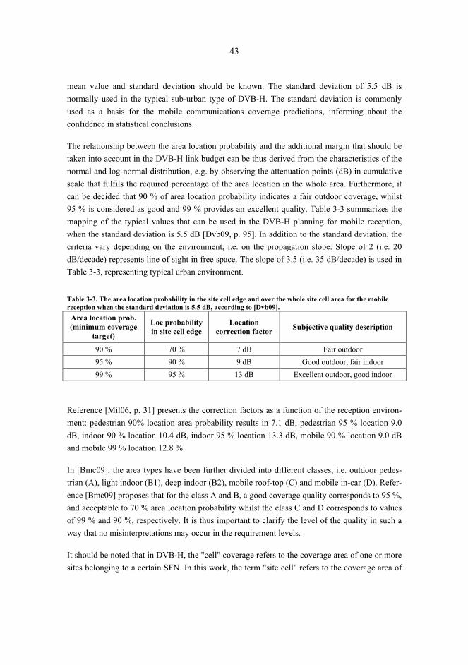
43

mean value and standard deviation should be known. The standard deviation of 5.5 dB is normally used in the typical sub-urban type of DVB-H. The standard deviation is commonly used as a basis for the mobile communications coverage predictions, informing about the confidence in statistical conclusions.

The relationship between the area location probability and the additional margin that should be taken into account in the DVB-H link budget can be thus derived from the characteristics of the normal and log-normal distribution, e.g. by observing the attenuation points (dB) in cumulative scale that fulfils the required percentage of the area location in the whole area. Furthermore, it can be decided that 90 % of area location probability indicates a fair outdoor coverage, whilst 95 % is considered as good and 99 % provides an excellent quality. Table 3-3 summarizes the mapping of the typical values that can be used in the DVB-H planning for mobile reception, when the standard deviation is 5.5 dB [Dvb09, p. 95]. In addition to the standard deviation, the criteria vary depending on the environment, i.e. on the propagation slope. Slope of 2 (i.e. 20 dB/decade) represents line of sight in free space. The slope of 3.5 (i.e. 35 dB/decade) is used in Table 3-3, representing typical urban environment.

Table 3-3. The area location probability in the site cell edge and over the whole site cell area for the mobile reception when the standard deviation is 5.5 dB, according to [Dvb09]. Area location prob. (minimum coverage

target)

Loc probability in site cell edge

Location correction factor Subjective quality description

90 % 70 % 7 dB Fair outdoor 95 % 90 % 9 dB Good outdoor, fair indoor 99 % 95 % 13 dB Excellent outdoor, good indoor

Reference [Mil06, p. 31] presents the correction factors as a function of the reception environ-ment: pedestrian 90% location area probability results in 7.1 dB, pedestrian 95 % location 9.0 dB, indoor 90 % location 10.4 dB, indoor 95 % location 13.3 dB, mobile 90 % location 9.0 dB and mobile 99 % location 12.8 %.

In [Bmc09], the area types have been further divided into different classes, i.e. outdoor pedes-trian (A), light indoor (B1), deep indoor (B2), mobile roof-top (C) and mobile in-car (D). Refer-ence [Bmc09] proposes that for the class A and B, a good coverage quality corresponds to 95 %, and acceptable to 70 % area location probability whilst the class C and D corresponds to values of 99 % and 90 %, respectively. It is thus important to clarify the level of the quality in such a way that no misinterpretations may occur in the requirement levels.

It should be noted that in DVB-H, the "cell" coverage refers to the coverage area of one or more sites belonging to a certain SFN. In this work, the term "site cell" refers to the coverage area of

44

a single antenna system of one transmitter. The antenna of the site cell can be omni-radiating or a set of directional antennas. The definition of the "cell" can be found in [Dvb09] which de-scribes that in the DVB-H system, the cell_frequency_link_descriptor indicates the frequencies that are used for the different cells of the network. The frequencies (and thus cells) are further-more mapped with Transport Streams. The cell_list_descriptor contains the needed information of the coverage area of the cells. Physically, cell is defined as a geographical area covered by the signals that contain one or more transport streams, which can be done with one or more transmitters. In the simulations of this thesis, the hexagonal model with omni-radiating antennas per site cell is used for the coverage estimate. In Publication V, though, sectorized site cells are used with realistic topological information about the surrounding areas in order to estimate the DVB-H coverage areas in dense urban area.

Path loss

The maximum path loss L (dB) is the difference between the effective isotropic radiating transmitter power PEIRP and the required received power in outdoors Pmin(out):

)min(outEIRP PPL −= (3-1)

In this formula, PEIRP (dBm) is:

TXpsccTXEIRP GLLPP +−−= (3-2)

The minimum received power level Pmin(out) (dBm) is:

GSMFECMPESFNlviout LGGLPP +−−+= −)min( , (3-3)

where Pi is the isotropic received power, Llv is the location variation for a certain area probabil-ity (that can be obtained from Table 3-3), GSFN is the SFN gain, GMPE_FEC is the MPE-FEC gain, and LGSM is the GSM filter loss due to the isolation of the DVB-H receiver and GSM transmitter.

The isotropic received power is obtained from:

RXRXi GPP −= min , (3-4)

where PRXmin is the receiver sensitivity, or the minimum power level the receiver requires, and GRX is the receiver's antenna gain. The latter depends on the frequency. Based on the informa-tion of [Dvb09, p. 87] a linear interpolation has been applied for {474 MHz < f < 858 MHz} for the antenna gain (which is in fact loss) throughout in the simulations of this thesis:

[ ] 172.16013.010384

47453845 −=−⋅−= ffdBiGRX (3-5)

The minimum required receiver's power level PRXmin is obtained by:

45

minmin )/( NCPP nRX += , (3-6)

where Pn is the receiver noise input power level, and (C/N)min is the minimum functional C/N which depends on the used modulation, CR and MPE-FEC rate.

The receiver noise input power Pn (dBW) can be presented further by:

)log(10 kTBFPn += , (3-7)

where F (dB) is the receiver's noise figure (component dependent) and Pt=10·log(kTB) is the thermal noise level, k is Boltzmann's constant 1.38·10-23 J/K, T is the temperature in Kelvin (290 K is normally used as an average value) and B is the receiver's noise bandwidth (Hz). In DVB-H, the value for B is 7.6 MHz in case of the 8 MHz variant. As an example, for the 8MHz band, the thermal noise floor is –105.2 dBm. Combined with the terminal's noise figure of 5 dB (this depends on the quality of the receiver's components, and it has frequency dependency), the Pn would be –100.2 dBm.

There is still one important item that should be taken into account when estimating the final maximum allowed path loss. This is the loss that the transmitter filter absorbs from the radiating power. In the general calculations, it can be estimated as 10% of the radiating power level (W). As an example, Publication I utilized the 10 % assumption for the transmitter filter loss. The effect can be taken into account when the transmitter power level is presented in dBm:

[ ] [ ]( )��

��

⋅⋅⋅= −3101

9.0log10 WPdBmP TXeffectiveTX (3-8)

The complete formula for the maximum path loss is thus:

[ ]( ) [ ] [ ] [ ] [ ] [ ][ ]( ) [ ] [ ]( )[ ] [ ]

[ ] [ ] [ ]dBLdBGdBGdBLdBMHzfdBNCdBmkTB

dBmNFdBiGdBLdBLdBmWPdBL

GSMFECMPESFN

lv

TXpsccTX

−+++−−+−+−

−−+−−��

��

⋅⋅⋅=

−

−

172.16013.0)/()log(1030101

9.0log10)(

min

3

(3-9)

Building loss

The building loss, or building penetration loss, can be estimated in a general level as an average value in different environment types, and it can thus be considered as a fixed radio link budget value for different area types. The DVB-H implementation guideline recommends a median value of 11 dB and a standard deviation value of 6 dB to be used for the building loss [Dvb09, p. 94]. In addition to the building penetration loss, i.e. the ratio of the average powers measured outside and inside the building with a fixed transmitter, also the building floor loss may be important to take into account in the detailed network planning. Reference [Jos07, p 3008] has concluded that the floor loss can be in certain cases approximately between 30 and 40 dB.

46

In [Bmc07], it is stated that the building loss is frequency dependent. This is logical as the radio wave penetrates into the buildings depending on the conditions. As an example, a typical urban building normally contains metallic supports that might create a Faraday cage. Depending on the wavelength of the signal and the hole-size of the supporting metal the respective attenuation varies. Reference [Bmc09, p. 12] includes typical building penetration losses for the general use of the radio link budget. They have been adjusted from the previous [Bmc07] link budget document. The updated table shows values of 7 dB for class D (in-car) for all the bands of VHF, UHF, L-band and S-band with no standard deviation. For the class B1 (light indoor), the pene-tration loss is given as 9 dB (with the standard deviation p of 4.5) for VHF, 11 dB (p = 5 dB) for UHF, 13 dB (p = 5 dB) for the L-band and 14 dB (p = 5 dB) for the S-band. For the class B2 (heavy indoor), the respective values are: 15 dB (p = 5 dB), 17 dB (p = 6 dB), 19 dB (p = 6 dB) and 19 dB (p = 6 dB).

The snap-shot measurements carried out during the field tests of Publication IX correlate with the above mentioned information. There were two building types investigated, first case (A) being an 8-floor hotel with an open centre area representing deep indoor (class B2), and the sec-ond (B) being a lighter 1-floor construction (class B1). In both cases, the received power level was stored with one-second interval in a slow-moving pedestrian radio channel type by walking outside of the building on the side where the transmitter antenna was installed, and then by re-peating the same measurements in the ground floor inside the centre of the building. A UHF frequency of 701 MHz was used in these measurements. The investigated buildings were lo-cated in a typical sub-urban area. It should be noted, that the building loss might vary consid-erably depending on the environment and building material. Figure 3-3 shows the cumulative normalized histogram of RSSI values for the first case (A). This format gives the 50-percentile of the indoor and outdoor. The graph is further post-processed from Figure 25 of Publication IX.

Building penetration loss

0102030405060708090

100

-49

-53

-57

-61

-65

-69

-73

-77

-81

-85

dB

Cum

ulat

ive

perc

enta

ge

IndoorsOutdoors

Figure 3-3. An example of the typical building loss in a format of a cumulative RSSI histogram, which is obtained by the difference of the received power in the indoor and outdoor area. This case represents the deep building type of B2.

47

The analysed results show that the difference in the average RSSI values of indoor and outdoor, i.e. the building loss, for the first case A, which represents the class B2, is 16.1 dB with the standard deviation of 5.8 dB in indoors and 3.9 dB in outdoors. The respective value set of [Bmc09, p. 12] is very close to this result, the difference between the measured one being about 1 dB. When comparing the building loss via the 50-percentile values the result would be about 18 dB. For the second case (B), which represents the class B1, the building loss that is calcu-lated via the differences of the average values, is 14.1 dB, with the standard deviation of 6.1 dB in outdoors and 2.9 dB in indoors. The difference between the [Bmc09] is now about 3 dB. The respective 50-percentile comparison indicates that the building loss is about 13 dB.

As both cases show differences between the average and respective 50-percentile values, it is important to define which the used method is for solving the building loss. In [Bmc09, p. 11], the average values are used, and the building penetration loss LP is obtained by comparing the signal level distributions E inside and outside of the building:

averageinaverageoutP EEL __ −= (3-10)

The examples presented in this thesis show that sufficiently amount of field tests clarifies the typical building loss values that can be used for the local adjustment of the link budget. Al-though only two snap-shot cases were investigated in Publication IX (shown in Publication’s Figure 25), they correlate with [Bmc09, p. 12] indicating that the respective building loss values can be used as default ones in the radio link budget until possible more in-depth local modifica-tion is made.

Effect of the antenna height: Receiver

The mobile environment affects on the coverage area of DVB-H differently compared to DVB-T. The planning assumption of the DVB-H radio link budget is outdoors with a 1.5 meter terminal height, typically in N-LOS in the city area. This causes a penalty for the DVB-H link budget compared to the DVB-T that is based on the fixed rooftop antenna with LOS [Far07]. Reference [Mil06, p. 32] indicates that the receiver antenna height loss can be 11 dB for rural area, 16 dB in suburban and 22 dB in urban area in Band IV. For the band V, the respective values are 13, 18 and 24 dB.

Effect of the antenna height: Transmitter

As Figure 3-4 and Publications I and V indicate, the height of the DVB-H transmitter site an-tenna has a key role in the coverage area of the DVB-H site cell. By observing Figure 3-4, the doubling of radiating power level, i.e. adding 3 dB to the radio link budget might raise the ra-dius of the site cell by about 30% in the typical DVB-H antenna heights, meaning that the cov-erage area would enhance around 70%. This could happen, e.g. by changing the 2400 W trans-mitter model to 4700 W model when using the antenna in 60 m height. On the other hand, if the

48

transmitter antenna height is moved from 60 m to 85 m (40% rise to the height) but using the same 2,400 W transmitter, the effect of the coverage area would be the same as doubling the transmitter power. This phenomenon should be considered in the cost optimisation of DVB-H.

SFN gain

One possible item in the radio link budget is the SFN gain that can enhance the performance in the overlapping areas, or provide the theoretical possibility to construct the sites further away from each others as the coverage area of each site cell rises. The interpretation of the benefit of SFN varies though.

The implementation guidelines [Dvb09, p. 78] mentions that there is a potential SFN diversity gain but without specifying more concrete values. The SFN gain in general has been noted as useful in [Zir00] and [Cha06]. On the other hand, [Bmc09, p. 15] recommends that the SFN gain would not be taken into account in the radio link budget. Nevertheless, the simulations car-ried out in Publication III show that the SFN gain is present in an SFN network that does not contain interfering sites (i.e. the distance of the extreme sites is within the distance determined by GI). Furthermore, Publication IV has concluded that as the number of the sites grows, the SFN gain rises to about 6 dB level in the theoretical case over a large SFN where the absolute signal power levels are summed in a completely non-interfered environment. With the parame-ter sets that results in smaller SFN sizes, as the number of sites grows, part of the sites may start to add interference thus reducing the SFN gain. Depending on the radio parameter set (FFT size and GI), the balance can still be achieved by adjusting the transmitter antenna heights and power levels, but some of the parameter values leads to the highly interfered network as shown via the simulations in Figures 6–7, 11–13 and 16–17 of Publication VII.

The challenge of using the SFN item in the link budget is that there is no coherent definition available for the gain. It could be interpreted as the difference between the received power lev-els in dB, comparing a single stream with a varying number of streams as has been presented in [Ple08]. The value could also be resolved by mapping the C/(N+I) distribution over the whole investigated area as has been presented in the simulations of Publications III, IV and X.

Minimum C/N

The minimum C/N ratio that is required for the successful reception of DVB-H video / audio streams depends on the combination of the modulation, code rate and MPE-FEC. Also the radio channel type has a clear effect. The information about the modulation and code rate dependency can be seen in [Dvb09] and [Bou06, p. 27]. The required carrier level values presented in these references have been used in the presented analysis throughout this thesis. It should be noted that as the values have been published in relatively early stage of DVB-H, they might not be the final ones, though, but as for the accuracy of the results presented in this thesis, it can be as-sumed that the values are sufficiently close to the reality for different channel types.

49

MPE-FEC

The MPE-FEC functionality has been designed to DVB-H in order to provide additional protec-tion for the radio transmission, which enhances the received signal quality. The MPE-FEC rate can be varied between 0�50%. According to [Dvb09, p. 14] MPE-FEC is suitable for the im-provement of the C/N performance in mobile radio channels. It also gives additional protection against the impulse noise, and enhances the performance of fast moving terminals by adding the Doppler shift resistance. The MPE-FEC gain depends on the environment. In general, the closer the radio channel is to the AWGN type, the less gain MPE-FEC offers. On the other hand, the MPE-FEC gain is more notable in the Rayleigh type of fast fading channel as the OFDM can utilize the separate radio components inside of the SFN area providing this additional gain.

Among various other references, [Him09] indicates a clear advantage in the use of MPE-FEC. The effect might be in order of several dB. In addition to the streaming services, MPE-FEC is also useful for the file-cast mode of DVB-H. According to [Gom07, p. 5], the needed time for the file transfer is considerably reduced, and more content can thus be delivered with the same infrastructure by utilising MPE-FEC. On the other hand, if the transmission time is kept the same, the area coverage for the reliable reception is enlarged. Publications II, VIII and X inves-tigates the behaviour of MPE-FEC by varying the radio parameter values and area types. The results correlate with the common understanding about the benefits of MPE-FEC. According to these results, depending of the parameter settings and radio channel type, the MPE-FEC can move the 5 % frame error rate point up to 7 dB in RSSI scale in the single site cell case, indi-cating that in the best case, the additional error correction can enhance considerably the link budget.

Other effects

The seasonal conditions might cause low-level yearly fluctuations in the radio propagation due to the variations of the moisture level of vegetation and weather conditions (e.g. via occasional tunnelling effects in the ionosphere). As an example, [Apa06a, p. 64] has noted that the field measurement results do have certain deviation due to the rain. It can be assumed though that in the typical link budget, the effect of the vegetation and rain is minimal for DVB-H in VHF/UHF bands. In case of the 1.6 GHz version, the effect might be more considerable due to the radio propagation characteristics in higher frequencies. In any case, the seasonal path loss variation can be considered as a minor detail in a practical radio link budget, and due to the challenges in the periodical adjustment of broadcast type of network, it is not necessary to take into account.

As another possible link budget item, the reception antenna diversity could be utilized to exploit the multipath propagation. According to [Bmc09, p. 15], this feature may not be implemented on all devices, though, so the diversity effect is not needed to be taken into account in the link budget until the penetration of the terminals containing possible receiver diversity or MIMO type of functionality is sufficiently high.

50

3.3.2 Propagation models

The most important radio related task in the nominal as well as in the detailed network planning is to estimate the DVB-H coverage area with the given parameters. There are various models available that are based on the radio propagation theories and experiments. There are also inter-polation methods presented [Bac04]. The outcome is typically a method that can be applied for the mathematical calculation of the estimated site cell radius. Some of the widely used experi-mental models in the mobile communications are based on the Okumura-Hata [Hat80], Cost 231-Hata [Cos99] and ITU-R [Itu07] path loss predictions. This type of models divides the for-mulation into separate area types, e.g. presenting urban, sub-urban and open areas. Cost 231-Walfisch-Ikegami based model is a slightly different as it tends to quantify the propagation en-vironment. Typically after the initial presentation of the models, there have been various valida-tion rounds that have confirmed the functionality, or have adjusted the models closer to the re-ality. As an example, the original Cost 231-Walfisch-Ikegami had a minor error in the initial presentation which was found later. Furthermore, the functionality of the model has been inves-tigated, e.g. in [Jeo01], which concluded that the results of the model are relatively close to the ones obtained from the Okumura-Hata based models especially when the building group height is close to the value of half of the street width.

The original Okumura-Hata path loss prediction model [Hat80] is useful in the approximate coverage estimation of DVB-H in many cases especially in the nominal radio network planning phase. As an example, the estimated path loss L (dB) in the large city type can be obtained by:

[ ] )lg()lg(55.69.44

)()lg(82.13)lg(16.2655.69)(

dh

hahfdBL

BS

MSBS i

−+

−−+= (3-11)

where hBS is the height of the DVB-H transmitter antenna (in range of 30–200 m), hMS is the height of the receiver (m), and d is the distance between the transmitting and receiving antennas (km). For the frequency range of 400–1500 MHz, the area type factor for the large city is:

( )( ) 97.475.11log2.3)( 2 −= MSLCMS hha (3-12)

The maximum distance d up to 20 km can now be obtained:

[ ]��

��

�

−

−−+−

= )log(55.69.44

)()lg(82.13)log(16.2655.69)(

10 BS

iMSBS

hhahfdBL

d (3-13)

For the medium-small city type, the correction factor is:

( ) ( )8.0log56.17.0log1.1)( −−−= fhfha mSMCMS (3-14)

For the sub-urban area type, the path loss L of (3-11) is used as a basis with the following:

51

4.528

log22

−��

��

��

��−=−

fLL urbansub (3-15)

Finally, the loss in the open area can be obtained by applying the following correction:

( ) 94.40log33.18log78.4 2 −+−= ffLLopen (3-16)

Figure 3-4 presents the estimated site cell range of the example calculated with the large city correction factor of the Okumura-Hata prediction model and by varying the transmitter antenna height and power levels according to Table 3-2. As can be noted, the antenna height has a major impact on the site cell radius compared to the transmitter power level.

Cell radius

0.0

2.0

4.0

6.0

8.0

10.0

12.0

14.0

20 40 60 80 100

120

140

160

180

200

Antenna height (m)

d (k

m)

P=1500WP=2400WP=3400WP=4700W

Figure 3-4. Examples of the DVB-H site cell radius, when 16-QAM, CR 1/2 and MPE-FEC 1/2 are applied. Neither the SFN gain nor MPE-FEC gain are utilised in these calculations.

Another suitable model for practically all DVB-H environments is ITU-R P.1546 [Itu07]. The model is based on pre-defined curves for the frequency range of 30 MHz to 3,000 MHz and for maximum antenna heights of 3,000 m from the surrounding ground level. The model is valid for terminal distances of 1 to 1,000 km from the base station over the terrestrial and sea levels, or for the combination of these.

If the investigated frequency or antenna height does not coincide with the pre-defined curves, the correct values can be obtained by interpolating or extrapolating the pre-defined values ac-cording to the annexes of [Itu07] and by applying the calculation principles presented in its An-nex 5. The case curves represent field strength values for 1 kW effective radiated power level (ERP), and the curves have been produced for the frequencies of 100 MHz, 600 MHz and 2

52

GHz. The curves are based on the empirical studies about the propagation. In addition to the graphical curve format, the values can be obtained also in a tabulated numerical format.

The ITU-R P.1546 method has been evaluated in different sources. Reference [Öst06] has con-cluded that in the rural area of Australia, P.1546-0 and P.1546-1 provide better overall predic-tion of the path loss compared to traditional models like Okumura-Hata. The comparison also shows that P.1546-2 on average underestimates the field strength by more than 10 dB in that area type. Nevertheless, it was shown that P.1546-2 improves the standard deviation of the pre-diction error compared to previous versions of the ITU-R P.1546. This result correlates with [Tun05] which has concluded that the accuracy of the ITU-R P.1546 is consistent with the Oku-mura-Hata model up to about 20 km for urban areas. For rural areas, the predicted field values of the ITU-R P-1546 model differ from the reference solution more than those of the older ITU models do. At the moment, the latest version of the model is ITU-R P.1546-3 [Itu07]. It was used in the simulation of the performance of a mountain site in Publication VII.

It can be assumed that the basic and extended versions of Okumura-Hata as well as ITU-R P.1546-3 models provide a sufficiently good first-hand estimate for the DVB-H coverage areas and respective capacity and quality levels in the initial network planning phase. These models have been designed for environments with antenna heights and site cell distances that fall into the typical assumptions of DVB-H networks. Reference [Mil06] identifies several other models, including ray-tracing type of estimates for the dense city centres. These models require more detailed digital map data with respective terrain height and cluster attenuations. In the most ad-vanced prediction models, a vector-based 3D map is needed. It logically has a cost effect on the planning but it increases considerably the accuracy of the coverage estimate. It can further be enhanced via local reference measurements by adjusting the model's estimate accordingly. As a cost-efficient compromise, 3D models could be utilised in the advanced phase of the radio net-work planning in the most important areas.

3.4 Safety distance [Publication VI] A preliminary calculation about the transmitter power levels should be carried out already in the initial radio network planning phase. In this stage, regulatory rules, as well as a rough estimate about EMC and safety zones give a base for estimating the minimum distance between DVB-H antennas and the surrounding population or the antenna systems of other telecommunication systems like GSM and UMTS.

In the initial phase of the radio network planning, it is sufficient to investigate the high level regulatory limits for the non-ionising radiation. A typical maximum allowed value for the DVB-H site might be in order of 50 kW (EIRP), with additional rules to be taken into account, e.g. as a function of the antenna height and site type (differentiating the wall-mounted, roof-top and

53

tower mounted antennas). The international and regional regulation provides sufficient infor-mation about the upper limits of the radiation that should be taken into account in the nominal plan. The radiation level might need to be limited further depending on the area type (urban or open), the antenna height, and the frequency. The practical limitations might mean that the highest power class transmitters and high-gain directional antennas can not be used in the im-plementation and the level should thus be revised case basis.

Detailed safety zone and EMC limit calculations can be carried out when the concrete site loca-tions are known. The allowed antenna distance from the other system antennas or from the in-stallation personnel and the population depends on the type of the installation, i.e. the limits vary depending on the rooftop, tower or indoor antenna placement. In a typical broadcast tower case, the main task is to calculate the EMC limitations, i.e. the interferences that DVB-H causes to other systems and vice versa, as the antennas are installed sufficiently high in towers by de-fault. In the roof-top and indoor installations, also the safety distance limits for the human expo-sure should be taken care of with related safety zone marking, e.g. for the occasional mainte-nance visits.

Publication VI presents studies about the safety distance calculations of the DVB-H installation in rooftops or towers. A simple yet functional model that is suitable for the DVB-H deployment is proposed in Publication VI for the safety distance estimates.

When the electrical field is calculated above or below the antenna, the attenuation factor of the vertical radiation pattern should be taken into account accordingly. The methodology applies in the close distance of the site, and the outcome is to minimize the interference level caused by DVB-H to the other systems nearby, as well as to make sure the human exposure limits are not exceeded. In the back-lobe of the antenna, the method proposes the use of the maximum value (i.e., the minimum possible attenuation value of the radiation pattern) over the whole half-hemi-sphere. Although the DVB-H frequency usage is regulated, there might also be need to calculate some special cases for the longer distances, like safety zones in the area where sensible space signal reception stations or military bases are present. In these cases, the related safety zone cal-culation is straightforward and the methodologies of, e.g. [Chu00] can be utilized.

In the site installations, it can be expected that the total exposure increases close to the sites due to the DVB-H. Field measurements presented in [Ple09, p. 332] show that in most of the loca-tions around the transmitter site, DVB-H is the dominating source of radiation. The methodol-ogy presented in Publication VI gives an estimate of the effect, and field tests can be performed in selected locations especially on the rooftop sites in order to fine-tune the calculations.

The outcome of the safety distance calculations in the nominal planning phase helps to reject those radiation levels from the planning assumptions that exceed the regulatory limits and are thus not possible to utilize in the detailed planning, either.

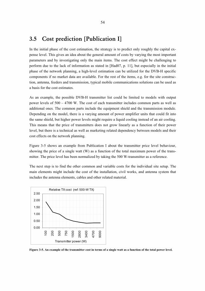
54

3.5 Cost prediction [Publication I] In the initial phase of the cost estimation, the strategy is to predict only roughly the capital ex-pense level. This gives an idea about the general amount of costs by varying the most important parameters and by investigating only the main items. The cost effect might be challenging to perform due to the lack of information as stated in [Had07, p. 11], but especially in the initial phase of the network planning, a high-level estimation can be utilized for the DVB-H specific components if no market data are available. For the rest of the items, e.g. for the site construc-tion, antenna, feeders and transmission, typical mobile communications solutions can be used as a basis for the cost estimates.

As an example, the possible DVB-H transmitter list could be limited to models with output power levels of 500 – 4700 W. The cost of each transmitter includes common parts as well as additional ones. The common parts include the equipment shield and the transmission module. Depending on the model, there is a varying amount of power amplifier units that could fit into the same shield, but higher power levels might require a liquid cooling instead of an air cooling. This means that the price of transmitters does not grow linearly as a function of their power level, but there is a technical as well as marketing related dependency between models and their cost effects on the network planning.

Figure 3-5 shows an example from Publication I about the transmitter price level behaviour, showing the price of a single watt (W) as a function of the total maximum power of the trans-mitter. The price level has been normalized by taking the 500 W-transmitter as a reference.

The next step is to find the other common and variable costs for the individual site setup. The main elements might include the cost of the installation, civil works, and antenna system that includes the antenna elements, cables and other related material.

Relative TX cost (ref: 500-W TX)

0.00

0.50

1.00

1.50

2.00

2.50

100

200

500

750

1500

2800

3400

4700

9000

Transmitter power (W)

Figure 3-5. An example of the transmitter cost in terms of a single watt as a function of the total power level.

55

The study can be done for the initial parameter set, i.e. according to the wanted capacity and the estimated average antenna heights. The coverage can be obtained for an individual site based on the suitable radio path loss prediction model. The cost of the network can thus be estimated by multiplying the expenses of a single site and the number of the site cells according to the single site cell radius.

As an example, the initial capacity target could be 5 Mb/s, which can be divided into a program guide (about 300 kb/s) and 10 channels consisting about 450 kb/s each for the combination of audio and video streams. As Table 3-1 indicates, this capacity requirement can be complied with the QPSK modulation, code rate of 1/2 and MPE-FEC rate of 2/3. Assuming that this mode requires C/N of 11.5 dB, and that the environment is urban vehicular with the coverage quality target for the location probability of 70% in the site cell edge and 90% in the site cell area, Table 3-4 can be created by applying the Okumura-Hata prediction model and the hexagonal site cell layout.

Table 3-4. The estimated site cell radius for a set of transmitter antenna heights hBS and transmitter power levels PTX by applying the Okumura-Hata model for the urban area.

Radius of the site cell (km) PTX (W)

hBS=30m hBS=60m hBS=90m hBS=120m

500 2.4 3.3 4.0 4.6 750 2.8 3.9 4.8 5.6

1500 3.4 4.8 6.0 7.1 2800 4.0 5.8 7.3 8.7

After the capacity and coverage analysis, the estimation of the expenses can be done. The cost of the single site can be calculated with the following Formula:

iablecommonsite CCC var+= (3-17)

Ccommon represents the fixed costs and it consists of the site civil and installation work as well as other costs that are constant independently of the power class. Cvariable consists of the transmitter cost (depending on the power level), feeder cost (which depends on the feeder length and on the type of the feeder which is selected based on the maximum supported power), and on other di-rectly related material that depends on the cable type / length and transmitter power level.

When taking the PTX = 500 W-case as a reference as shown in Figure 3-5, the cost for the trans-mitters with 500, 750, 1500 and 2800 W is now 1, 0.6, 0.5 and 0.45, respectively. The unit cost per meter of the antenna feeder is estimated in this analysis by comparing it with the normalized cost of 500W transmitter. In a practical case, the costs can logically be expressed in absolute commercial values of each item.

56

It is now possible to estimate the approximate cost for each site combination in order to build sufficient amount of sites in a certain area. The total cost is thus:

Asitetot NCC ⋅= , (3-18)

where NA is the total amount of sites in the area A.

As an example, the A could be selected as 100×100 km2. The radius of the site cell for, e.g. 500 W-case and antenna height of 30 m is 2.4 km. The ideal overlapping in the hexagonal model can be taken into account as shown in the network layout calculation of Annex I. Based on this information it is possible to calculate the number of the partially overlapping sites in the inves-tigated area as shown in Table 3-5.

Table 3-5. The total number of sites in the planned area.

PTX (W) hBS=30m hBS=60m hBS=90m hBS=120m

500 1113.1 574.8 379.6 279.5 750 884.2 450.4 294.9 215.7

1500 596.5 296.9 191.5 138.5 2800 418.5 203.9 129.8 92.9

When investigating further the cases, the unit cost of the sites can be obtained per transmitter power level category as shown in Table 3-6. The information represents a snap-shot example of certain transmitter vendor's different models when they are compared with the 500 W-model of this specific provider. It should be noted that the relative comparison depends on each case.

Table 3-6. An example of the unit cost of the sites for a set of power categories.

PTX (W) Normalized cost

500 1.00 750 0.60 1500 0.50 2800 0.45

In this analysis, an assumption for the impact of the cable length on the costs can be rejected. As a next step, the normalized cost per transmitter category can be obtained. Table 3-7 shows the cost of the solution as a function of the antenna height in the investigated area. In this analysis, the cost effect of the towers is not considered as the assumption of the cost calculation is to use already existing ones.

57

Table 3-7. The normalized cost for different parameter values in order to cover 100×100 km2. PTX (W) hBS=30m hBS=60m hBS=90m hBS=120m

500 1113.1 574.8 379.6 279.5 750 530.5 270.2 176.9 129.4

1500 298.3 148.4 95.7 69.2 2800 188.3 91.8 58.4 41.8

As can be noted from Table 3-7, by using only the basic parameters, we can note the cost effect of the antenna height compared to the transmitter power category. As can be seen in Table 3-7, the 1500 W transmitter solution with the antenna installed in 120 m comes more attractive than 2800 W transmitter with the antenna installed to 60 m height.

As the CAPEX analysis shows, the strategy for the antenna height and transmitter power cate-gory should be done in a sufficiently in-depth level in order to make sure the optimal combina-tions of the parameter values and respective costs. At the initial planning phase, though, a rough estimation is sufficient in order to understand the cost-effect of different solutions as presented above.

The starting point of the technical parameter designing in the very initial phase of the network planning is the selection of the transmitter type. Table 3-8 summarises the most important as-pects that should be taken into account in the techno-economic cost optimization when the transmitter strategy is decided.

Table 3-8. The summary of pros and cons of DVB-H transmitter power levels. Transmitter type Benefits Drawbacks

Low power − Low energy consumption. − Economical and easy to install and

maintain. − The installation is possible also in

rooftop sites due to the smaller safety zones.

− Single site coverage small which requires high number of sites. The obtaining of sites is not straightfor-ward in practice.

− High transmission costs in case of terrestrial solution.

High power − Low number of transmitters which results in the easier site candidate planning and the actual obtaining of sites.

− The network can be build up rela-tively fast.

− Provides large coverage areas espe-cially in relatively open area and if the antenna can be installed high.

− Power consumption rises exponen-tially as the transmitter power is higher.

− Liquid cooled transmitter needs additional maintenance.

− The outages in coverage if obstacles (especially in urban areas) which requires additional gap fillers.

− A single site breakdown causes a large service outage.

58

The high-level cost estimate is important to include already in the nominal planning phase in order to reject the least feasible parameter values and materials. In the detailed network dimen-sioning and optimisation phase, also the CAPEX analysis should be more in-depth. In that phase, the OPEX should be taken into account, as the importance of the operating costs of the network might rise considerably during the operational years of the network. In that phase, the more thorough investigation of the items that have cost effect should be carried out. The respec-tive methodology is presented in Publication I and Chapter 5.3 of this thesis.

59

4 Detailed radio network design

4.1 Identifying the planning items

In the detailed network dimensioning, the aim is to find the optimal balance of all the relevant items that have effect on the network performance and costs. There are various different pieces of information and investigations available describing the possible sub-tasks of DVB-H network planning, including technical parameter effects, economical and regulation aspects as shown in [Dvb09], [Gre06], [Apa06a], [Apa06b], [Bee07], [Far06], [Had07], [Him09], [Mil06], [Ung08], [Apt06], [Ecc04], [Bro02] and [Min99].

Based on the above mentioned sources as well as on the field tests, analysis and simulations carried out in Publications I–X, a complete process of the planning aspects and their relations was formed as an initial part of this thesis. Figure 4-1 shows the outcome of the investigations, i.e., the main topics to be considered as a basis for the detailed DVB-H network planning phase.

The balancing of the radio network performance can be done by investigating and dimensioning the cross-relations of technical, economical and regulatory items in a deep level. The ultimate goal of the detailed DVB-H radio network dimensioning is to find the cost-efficient balance between the coverage, capacity and the quality by taking into account the relevant parameters.

There might be several optimal points for the balance, i.e. several different combinations of the parameter values could result in the same optimal solution technologically. Whilst the suffi-ciently good balance is found, it does not matter what is the theoretical set of solutions. The practical restrictions can determine though the perfect solution. As an example, even if different number of sites could produce the same optimal solution by varying several radio parameter values, the lower amount of sites could be more practical as the obtaining of the site locations is not straightforward task in practice. As an example, it might not be always possible to purchase or rent a site in the technically most suitable location due to the practical reasons that are not always predictable in the network design.

The ideal network dimensioning takes into account the future enhancement needs. It is thus im-portant to make sure that the service areas are not reduced in the later phases. As an example, if the coverage area is done with QPSK providing large operational areas but with low capacity, the preferable aim should be that if the modulation is switched to 16-QAM which provides more capacity but with a lower coverage area per site, there are sufficient amount of gap-fillers and additional main sites operating in the critical areas, so that the customers would not experience a degradation of the services.

60

The mature network operation phase requires technical optimisation, which might be a continu-ous process even in a stable network. The optimisation can be done by carrying out field meas-urements in selected, most relevant areas of the network. The correct measurement methodology as well as the right interpretation of the measurement data is important in this phase.

Capacity

Coverage

SFN gain /SFN interferences

-FFT, GI

Over-sized SFN

Standard SFN

SFN gain level-overlapping

MFN

MFN functionality-signalling speed,

overlapping

Effect of network type

Site performance

Antenna height

TX power

Regulatory limitations

EMC/Safety distance

Frequency coord.OPEX

Economical limitations

CAPEX

Correction capability

MPE-FEC

Code rate

User experiences

CH switching time

Reception quality

Bit/frame rates

Performance

Measurements

Fault Management

Analysis

Link budget

Publication I Publication VI

Publications II, IX

Publication VIIIPublications III, IV, X Publications V, VII

Capacity

Coverage

SFN gain /SFN interferences

-FFT, GI

Over-sized SFN

Standard SFN

SFN gain level-overlapping

MFN

MFN functionality-signalling speed,

overlapping

Effect of network type

Site performance

Antenna height

TX power

Regulatory limitations

EMC/Safety distance

Frequency coord.OPEX

Economical limitations

CAPEX

Correction capability

MPE-FEC

Code rate

User experiences

CH switching time

Reception quality

Bit/frame rates

Performance

Measurements

Fault Management

Analysis

Link budget

Publication I Publication VI

Publications II, IX

Publication VIIIPublications III, IV, X Publications V, VII

Figure 4-1. The cross relations of the items affecting on the DVB-H radio dimensioning. In this diagram, the final aim is the balancing of the capacity and coverage by taking into account the restrictions and enhance-ments related to the technology, commercial and regulatory items.

4.2 Detailed network planning process

Figure 4-2 presents the needed steps of the detailed DVB-H radio network planning process based on the identified topics of Figure 4-1. The detailed process was developed as a part of this thesis in order to seek for the relevant study items. It is a continuum of the nominal planning phase, and it is meant for adjusting the higher level planning assumptions by identifying the items that may change the coverage, capacity and quality of the radio network compared to the original plan.

61

Optim

isatio

nMe

asur

emen

ts, us

er ex

perie

nces

Capacity planningRevise / confirm the capacity requirement per SFN area => tune

parameters if needed

Decision of the site locationsSite candidates e.g. in rooftops, BC or telecom towers => confirm / adjust

the preferable set

Coverage planning IRadio planning program: Adjust antenna heights, transmitter powers per

site => estimate the radius per site cell

Coverage planning IISFN interference analysis to adjust coverage accordingly.

Is the interference and radiation level sufficiently low?No Yes

Cost planningAdjust the cost prediction according to the detailed coverage plan (detailed

CAPEX/OPEX optimization).Acceptable level of costs?

No Yes

Coverage planning IVRevise that coverage fulfils the requirements (with x % area/location

probability) and sufficient overlapping existsNo Yes

Initial planning process

End of planning process

Coverage planning IIIMFN analysis to adjust coverage accordingly.Is there sufficient overlapping for handovers?

No YesOp

timisa

tion

Meas

urem

ents,

user

expe

rienc

es

Capacity planningRevise / confirm the capacity requirement per SFN area => tune

parameters if needed

Decision of the site locationsSite candidates e.g. in rooftops, BC or telecom towers => confirm / adjust

the preferable set

Coverage planning IRadio planning program: Adjust antenna heights, transmitter powers per

site => estimate the radius per site cell

Coverage planning IISFN interference analysis to adjust coverage accordingly.

Is the interference and radiation level sufficiently low?No Yes

Cost planningAdjust the cost prediction according to the detailed coverage plan (detailed

CAPEX/OPEX optimization).Acceptable level of costs?

No Yes

Coverage planning IVRevise that coverage fulfils the requirements (with x % area/location

probability) and sufficient overlapping existsNo Yes

Initial planning process

End of planning process

Coverage planning IIIMFN analysis to adjust coverage accordingly.Is there sufficient overlapping for handovers?

No Yes

Figure 4-2. The detailed planning phase contains in-depth analysis of the effects of the performance parame-ters. The steps can be iterative.

In the operational phase of the network, a continuous optimisation may take place via the field testing and customer feedback. The optimisation includes the performance monitoring as well as the fault management in case the planned coverage changes, e.g. due to the faulty antenna that does not trigger alarm for the operations and management system.

The proposed model can be considered as an enhanced version compared to typical processes presented in publicly available sources due to the including of the cost planning and optimisa-tion modules. As an example, [Ebu05] and [Dvb09] describe in detailed level different aspects of the network planning, but they do not present a complete DVB-H planning process.

62

4.3 Capacity planning

In the detailed phase of the radio network dimensioning, the capacity planning methodology does not change much compared to the one presented in the initial phase. The principle remains the same, but the balancing of the capacity and coverage, i.e. the number of the sites and related costs might need several iteration rounds.

The provided capacity does have a direct relation with the cash flow of the operational network. The end-user requires normally several channels to choose from, and the quality of each one should be in acceptable level, taking into account the content type of the channels. The balanc-ing of the number of channels and the bit rate of each one is relatively flexible in DVB-H. There can be several different bitrates defined for different channels, i.e. there could be low bit rate channels for audio news type of service, whilst the highest resolution and audio quality might be required, e.g. for music video channels. The upper limit for the dimensioning is determined by the bandwidth, which can be divided for several sub-channels.

4.4 Coverage planning [Publications V, VII]

4.4.1 Effect of site locations

In the initial phase of the coverage planning, a rough estimation of the number of the sites is needed. The estimation can be done by carrying out a theoretical estimation of the overall path loss to different environments, e.g. urban and dense urban, sub-urban and rural/open areas. The estimation can be done by filling in the planned areas, e.g. by hexagonal type of site cells. Al-though this approach is theoretical, it gives a first estimation about the needed sites. If the aver-age site antenna height and the transmitter power level are close to the reality, the prediction is sufficiently good for the nominal planning purposes.

In the detailed planning phase, the more accurate site locations should be known. This is the most challenging part of the coverage planning, as the practical sites can rarely be found in the ideal locations according to the uniform type of the initial network layout. In addition, there might be restrictions in the antenna height and transmitter power level usage. As an example, the already existing broadcast or mobile communications towers are normally equipped with other antennas of various systems, as GSM, UMTS, radio, TV and link antennas, which might prevent the additional installations due to the EMC restrictions.

The variation of the practical antenna heights and transmitter power levels affects on the optimal CAPEX and OPEX calculations, so the techno-economical analysis should be done accordingly in order to find the proper balance for the radio parameter values and the network cost.

63

In order to provide positive user experiences, the coverage areas should be overlapping. In the SFN network, this results in the additional SFN gain, which does have effect on the perform-ance via the link budget enhancement [Ebu05]. In case of the MFN, the sufficiently overlapping areas provide the handover functionality without problems.

4.4.2 Site cell range predictions

When the final site locations are known, the detailed coverage estimation can be done. The se-lection of the suitable radio propagation prediction model is important, and in the detailed analysis, a local adjustment of the propagation model parameters is recommendable. The latter can be done by carrying out field measurements and by correlating results with predictions, and correcting the propagation model’s parameter set (e.g. by tuning clutter attenuation values).

In the detailed phase of the network coverage planning, the possible SFN interference level should be investigated thoroughly. If the theoretical SFN limits are not exceeded, it is straight-forward to assume that there are no interferences present. If reflections are expected from dis-tant obstacles, they increase the effective delay of the radio components and the probability of the occurrence of interferences increases.

In case of interferences, the path loss prediction method, i.e. analysis to estimate the carrier lev-els as a function of the geographical location, should include also the interference analysis. One possibility is to integrate the method shown in Publications III, IV, VII and X into the tradi-tional radio planning program.

As for the sole coverage within non-interfered SFN area, Publication V shows examples about the commercial planning tool's (NetAct Planner) prediction model usage in urban and dense urban environment. The model of the NetAct Planner is based on the Okumura-Hata [Hat80], which also takes into account the local clutter attenuation factors. As the used map resolution in the presented cases studies is in order of 30 meters, it does not provide the most accurate cover-age prediction, e.g. inside the street canyons. Nevertheless, the model is sufficiently accurate for planning purposes especially in sub-urban areas, like Publication V has been concluded.

NetAct Planner is typically utilized in the 2G and 3G mobile network coverage predictions, and can be adapted to the basic DVB-H coverage prediction by applying the same principles. Vari-ous different models can be utilized as a base of the predictions, including the more accurate ray-tracing based 3-dimensional models. If the Okumura-Hata model is utilized, the basic out-come of the tool's propagation model is further enhanced by taking into account additional at-tenuation values that depend on a separate cluster map of the investigated area. Several different cluster types can be defined, e.g., for the water areas and forests with different vegetation densi-ties. The cluster values can be further adjusted by comparing the prediction of different area types with the field test results. If the attenuation values of the clusters are estimated well

64

enough, this method results in more realistic predictions compared to the sole Okumura-Hata model that generalizes the prediction solely over different city and rural environments. Never-theless, as Publication V concludes, the basic Okumura-Hata model as such indicates the needed number of the sites per area type sufficiently accurately for the nominal planning purposes.

In practice, according to [Mil06, p. 17], there might be well over 20 taps in the radio channel. This should be taken into account in the deep level radio network planning and analysis. The recommendation of [Mil06, p. 17] is to use at least 12 taps for the respective simulations al-though the practical terminal deployment would not take the full advantage of all these compo-nents. The basic coverage area is studied in [Mil06, p.66]. The outcome correlates with the analysis done in Publication V, although the studies represent different densities of the urban area types.

The balance between the economical aspects and technical solutions depends highly on the wanted quality of the service level. It is thus logical to decide an initial target for the network's coverage and capacity, and to investigate with what parameter combinations the target could be achieved. The detailed network planning might require several iteration rounds depending on the outcome, i.e. if the network cost in initial and longer term turns out to be expensive even in the technically optimal point.

The main idea of this thesis is to investigate the useful coverage area that is a result of the basic link budget and area dependent propagation models, added by the possible MPE-FEC and SFN-gain and which is reduced by the possible SFN interference in the over-sized SFN. The found sources typically do not consider this type of complete vision at the same time but concentrates on the selected details [Bac04] [Bmc09] [Bro02] [Ecc04] [Fan06a] [Fan06b] [Far01] [Fcc07] [Goe02] [Gre06] [Hum09] [Mar05] [Pal08] [Sil06] [Tun05] [Ung06] [Wan03] [Zha06] [Zha08] [Zyr98].

4.5 Local measurements [Publications II, VIII, IX] The field measurements are needed for the revisions of the performance level of DVB-H. As DVB-H is a broadcast system without its own uplink channel, the terminals themselves cannot be used directly as reporting devices. The field measurements provide data for the performance analyse as well as for the fault management.

Other usage of the field measurements is related to the radio propagation prediction model ad-justment of DVB-H. The received power level combined with the location information can be utilised in the typical planning programs in order to correlate and correct the model parameter values, e.g. the cluster attenuation values. The correction can normally be made either manually or automatically.

65

When the field measurements are initiated, it is important to calibrate the equipment. Publica-tion IX, Figure 21 shows an example of the differences in the channel display when three differ-ent DVB-H terminal units are used as measurement equipment. Figure 4-3 shows the further processed cumulative presentation of the differences of the channel displays. As can be seen, the 50%-ile point results in �57.3 dBm, �58.8 dBm and �61.2 dBm for each terminal.

CDF, P(RX) of 3 terminal displays

0.00.10.20.30.40.50.60.70.80.91.0

-70

-67

-64

-61

-58

-55

-52

-49

-46

-43

-40

RSSI (dBm)

MS1MS2MS3

Figure 4-3. Comparison of the RSSI display of 3 different DVB-H terminals used in Publication IX. Cumulative distribution of the laboratory measurement with 90 samples per terminal.

In the field measurements described above, the terminal’s already existing field test program displays the received power level based on the interpretation of the gain values of the automatic gain control (AGC). The minimum step size of the AGC tends to be typically in order of 1 dB. The accuracy of this method is approximately 1...2 dB depending on the received power range [Aur09]. If a power meter is used instead, the accuracy is roughly in the same order. In addition, the quality of the calibration affects on the final estimate of the received power level. The importance of the calibration has been noted also in [Apa06a, p. 20] which describes the challenge in the interpretation of field tests when high accuracy is required.

In order to minimize the inaccuracy of the channel display, the corresponding calibration can be carried out, e.g. by installing a coaxial cable directly to the input of the DVB-H receiver and by connecting a TS generator to it [Aur09]. If instead more advanced field or laboratory equipment like spectrum analyzer is used as in [Jos07], the accuracy of the averaged samples is logically more reliable. There are also other measurement criteria like error vector that can be utilized in the signal-to-noise ratio calculations as presented in [Fan06a, p. 33]. Nevertheless, the main idea of the presented field test methodology is based on a portable device which can collect suffi-ciently accurate measurement data in all the user environments, including indoors, without the need to connect it to the external power supply.

66

4.5.1 Coverage area

The basic coverage area can be studied by observing the received power level PRX of the site cell around the functional coverage limit as presented in Figure 4-4. The receiving of the radio sig-nal can be done with a scanner using respective bandwidth and averaging settings, or with a terminal capable of showing the radio parameter values as explained in Publications II, VIII and IX. In the analysis, it is important to understand the effect of the averaging of the samples dur-ing the measurement. If a real audio / video stream can be transmitted, a normal DVB-H re-ceiver can be used as parallel equipment for the subjective quality check. This method would be sufficient in the very initial phase of the planning, in order to understand the parameter value behaviour on the quality of the received contents.

Received power level

-90

-85

-80

-75

-70

-65

-60200 400 600 800

Sample #

RS

SI (

dB)

Figure 4-4. An example of the collected received power levels by moving the receiver close to the functional cell edge. The received power level samples and corresponding geographical locations can be observed by post-processing the measurement data to a map format which indicates the expected coverage limits.

One of the aims of the radio coverage measurements is to revise the accuracy of the applied prediction models in the investigated area type. Based on the received power level distribution, the respective model adjustment can be made by adjusting the outcome of the prediction with the offset the field measurements provide. Depending on the model the area cluster attenuation factors can be modified as it is one of the main items that affect on the accuracy of the predic-tions.

It should be noted that the accuracy of the received power level measurement depends on the equipment. As shown in Publication II, the DVB-H terminals can be used well for the fast revision of the basic coverage, but the respective accuracy of the analysis suffers about 2 dB additional margin due to the lack of calibration of the field strength displays.

67

For the more in-depth revision of the achieved quality levels as a function of the received power level requires deeper analysis which is presented in the following Chapter 4.5.2. The method is based on the data collection from the field and on the respective post-processing.

4.5.2 Error correction

Publications II, VIII and IX show the methodology for the field measurements and their analysis in order to find the detailed level of information about the performance of the network. For the optimisation of the network performance, basic field strength measurements are important to carry out in an early phase of the network deployment, by observing the functional limits via the measurement equipment, e.g. with a GPS receiver producing the location information for the measurement results. Publication IX describes the more in-depth quality measurements and re-spective results for resolving the QEF, FER and MFER breaking points for different operational modes of DVB-H.

In the method presented in Publications II, VIII and IX, the frame error rate has been identified as a useful criterion when the basic performance indicators can be collected from the air inter-face. This is logical as the end-users experiences the quality level variations in the real-time de-pending on the correctness of the received frames.

The method shows that the quality can be analyzed by arranging the collected FER and MFER occurrences as a function of the received power level. The MPE-FEC gain can be obtained when the results are converted into a cumulative distribution format. As the resolution of the presented equipment is 1 dB for the received power level, the corresponding proportion of error-free frames, frames that can be corrected with MPE-FEC and the ones that remain erroneous can be normalized per each RSSI category. In this way, the breaking point of the observed criterion of MPE-FEC and FEC is possible to obtain. When this method is utilised, it is important to col-lect a sufficient amount of measurement data for the statistical reliability. According to [Dvb09, p. 83] the accuracy of the frame error rate would be sufficient if at least 100 samples are col-lected. These samples include both error-less and erroneous MPE-FEC frames.

The FER information, i.e. frame errors before MPE-FEC specific analysis, is obtained after the Time Slicing process, and the MFER is obtained after the MPE-FEC module. If the data after MPE-FEC is free of errors, the respective data frame is de-encapsulated correctly and the IP output stream can be observed without disturbances. As the erroneous frame indicates directly the user perception of the quality, the frame error rate before and after MPE-FEC are useful in-dicators for the performance studies. As stated in [Dvb09, p. 83], an erroneous frame destroys the service reception for the whole interval between the time-sliced bursts.

According to [Dvb09, p. 83] the 5 % FER / MFER can be considered as a criterion for the ac-ceptable quality level. This point can be studied in various ways. One method is to collect suffi-

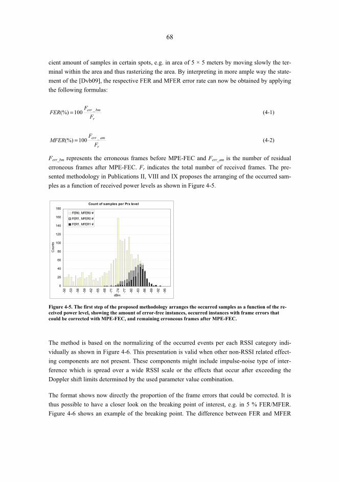
68

cient amount of samples in certain spots, e.g. in area of 5 × 5 meters by moving slowly the ter-minal within the area and thus rasterizing the area. By interpreting in more ample way the state-ment of the [Dvb09], the respective FER and MFER error rate can now be obtained by applying the following formulas:

r

bmerr

FF

FER _100(%) = (4-1)

r

amerr

FF

MFER _100(%) = (4-2)

Ferr_bm represents the erroneous frames before MPE-FEC and Ferr_am is the number of residual erroneous frames after MPE-FEC. Fr indicates the total number of received frames. The pre-sented methodology in Publications II, VIII and IX proposes the arranging of the occurred sam-ples as a function of received power levels as shown in Figure 4-5.

Count of samples per Prx level

0

20

40

60

80

100

120

140

160

180

-50

-53

-56

-59

-62

-65

-68

-71

-74

-77

-80

-83

-86

-89

-92

-95

dBm

Cou

nts

FER0, MFER0 #

FER1, MFER0 #

FER1, MFER1 #

Figure 4-5. The first step of the proposed methodology arranges the occurred samples as a function of the re-ceived power level, showing the amount of error-free instances, occurred instances with frame errors that could be corrected with MPE-FEC, and remaining erroneous frames after MPE-FEC.

The method is based on the normalizing of the occurred events per each RSSI category indi-vidually as shown in Figure 4-6. This presentation is valid when other non-RSSI related effect-ing components are not present. These components might include impulse-noise type of inter-ference which is spread over a wide RSSI scale or the effects that occur after exceeding the Doppler shift limits determined by the used parameter value combination.

The format shows now directly the proportion of the frame errors that could be corrected. It is thus possible to have a closer look on the breaking point of interest, e.g. in 5 % FER/MFER. Figure 4-6 shows an example of the breaking point. The difference between FER and MFER

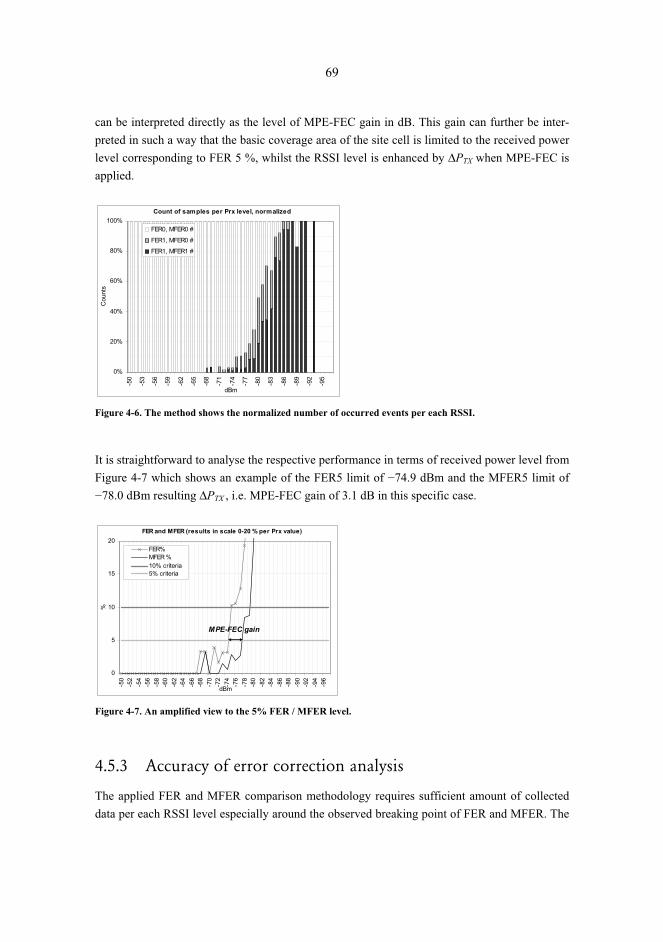
69

can be interpreted directly as the level of MPE-FEC gain in dB. This gain can further be inter-preted in such a way that the basic coverage area of the site cell is limited to the received power level corresponding to FER 5 %, whilst the RSSI level is enhanced by ΔPTX when MPE-FEC is applied.

Count of samples per Prx level, normalized

0%

20%

40%

60%

80%

100%

-50

-53

-56

-59

-62

-65

-68

-71

-74

-77

-80

-83

-86

-89

-92

-95

dBm

Cou

nts

FER0, MFER0 #

FER1, MFER0 #

FER1, MFER1 #

Figure 4-6. The method shows the normalized number of occurred events per each RSSI.

It is straightforward to analyse the respective performance in terms of received power level from Figure 4-7 which shows an example of the FER5 limit of �74.9 dBm and the MFER5 limit of �78.0 dBm resulting ΔPTX , i.e. MPE-FEC gain of 3.1 dB in this specific case.

FER and MFER (results in scale 0-20 % per Prx value)

0

5

10

15

20

-50

-52

-54

-56

-58

-60

-62

-64

-66

-68

-70

-72

-74

-76

-78

-80

-82

-84

-86

-88

-90

-92

-94

-96

dBm

%

FER%MFER %10% criteria5% criteria

MPE-FEC gain

Figure 4-7. An amplified view to the 5% FER / MFER level.

4.5.3 Accuracy of error correction analysis

The applied FER and MFER comparison methodology requires sufficient amount of collected data per each RSSI level especially around the observed breaking point of FER and MFER. The

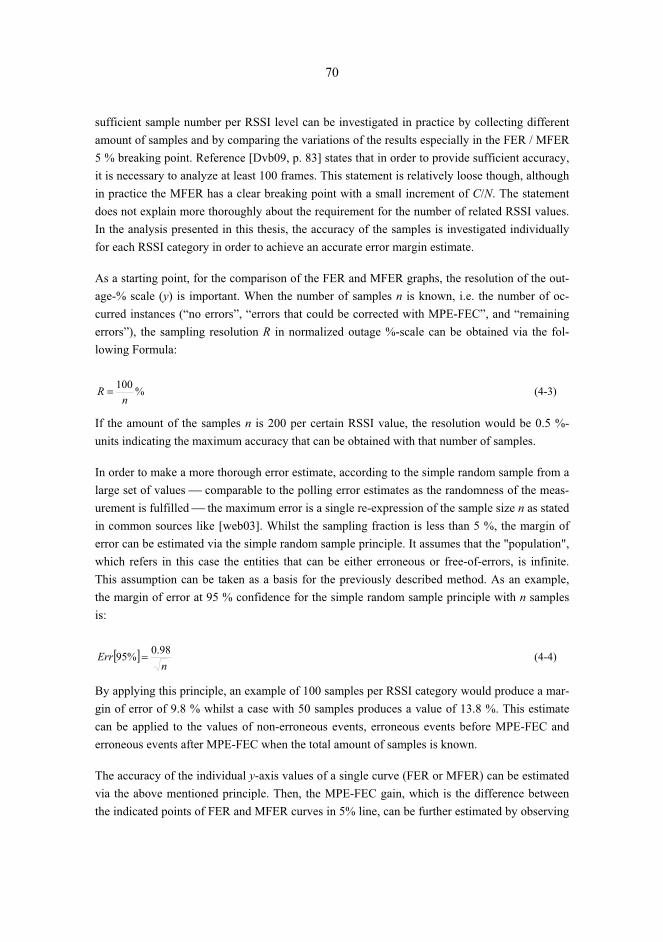
70

sufficient sample number per RSSI level can be investigated in practice by collecting different amount of samples and by comparing the variations of the results especially in the FER / MFER 5 % breaking point. Reference [Dvb09, p. 83] states that in order to provide sufficient accuracy, it is necessary to analyze at least 100 frames. This statement is relatively loose though, although in practice the MFER has a clear breaking point with a small increment of C/N. The statement does not explain more thoroughly about the requirement for the number of related RSSI values. In the analysis presented in this thesis, the accuracy of the samples is investigated individually for each RSSI category in order to achieve an accurate error margin estimate.

As a starting point, for the comparison of the FER and MFER graphs, the resolution of the out-age-% scale (y) is important. When the number of samples n is known, i.e. the number of oc-curred instances (“no errors”, “errors that could be corrected with MPE-FEC”, and “remaining errors”), the sampling resolution R in normalized outage %-scale can be obtained via the fol-lowing Formula:

%100n

R = (4-3)

If the amount of the samples n is 200 per certain RSSI value, the resolution would be 0.5 %-units indicating the maximum accuracy that can be obtained with that number of samples.

In order to make a more thorough error estimate, according to the simple random sample from a large set of values ⎯ comparable to the polling error estimates as the randomness of the meas-urement is fulfilled ⎯ the maximum error is a single re-expression of the sample size n as stated in common sources like [web03]. Whilst the sampling fraction is less than 5 %, the margin of error can be estimated via the simple random sample principle. It assumes that the "population", which refers in this case the entities that can be either erroneous or free-of-errors, is infinite. This assumption can be taken as a basis for the previously described method. As an example, the margin of error at 95 % confidence for the simple random sample principle with n samples is:

[ ]n

Err 98.0%95 = (4-4)

By applying this principle, an example of 100 samples per RSSI category would produce a mar-gin of error of 9.8 % whilst a case with 50 samples produces a value of 13.8 %. This estimate can be applied to the values of non-erroneous events, erroneous events before MPE-FEC and erroneous events after MPE-FEC when the total amount of samples is known.

The accuracy of the individual y-axis values of a single curve (FER or MFER) can be estimated via the above mentioned principle. Then, the MPE-FEC gain, which is the difference between the indicated points of FER and MFER curves in 5% line, can be further estimated by observing

71

the extreme values of the accuracy of the single curve. As an example, a measurement result of Publication IX can be analysed. Let’s select a case of {16-QAM, CR 2/3, MPE-FEC 2/3, GI 1/4, FFT 4K}, which produced the sample distribution as shown in Figure 4-8.

Samples per Prx level

0

20

40

60

80

100

120

-50

-54

-58

-62

-66

-70

-74

-78

-82

-86

-90

-94

RSSI (dBm)

# of

sam

ples

FER0, MFER0 #FER1, MFER0 #FER1, MFER1 #

Figure 4-8. An example of the collected data distribution over the RSSI scale.

Table 4-1 summarises the occurred total amount of samples per RSSI category and shows the respective margin of error for 95 % confidence by applying the above mentioned formulas. As can be seen, the accuracy of the RSSI levels of �70 dBm and �71 dBm is not sufficient, but Figure 4-8 indicates that even if the respective number of total samples is low for these RSSI categories, the received power level has been clearly sufficient for error-free functioning. It can be seen from the margin error analysis that the MFER5 can be found between RSSI levels of �76 dBm and �77 dBm when the confidence level of 95 % is applied.

Let us observe the RSSI scale of �70…�80 dBm by analyzing individually the error margin for each RSSI category in such a way that the total number of occurred events, i.e. “error-free” (FER0, MFER0), “FEC resulting error but MPE-FEC has corrected” (FER1, MFER0) and “error after MPE-FEC” (FER1, MFER1) is taken into account for the error margin calculation.

Figure 4-9 shows the result of the analysis with respective marginal for each respective FER and MFER value. When the FER5 and MFER5 is observed, FER5 results in values of PRXmin = �71.9 dBm, PRX = �72.1 dBm and PRXmax = �72.3 dBm. MFER results in PRXmin = �76.3 dBm, PRX = �76.4 dBm and PRXmax = �76.5 dBm dBm. The respective MPE-FEC gain can thus be informed as �76.4 � (�72.1) dBm = 4.3 dB with the value range of [4.0, 4.6], taking into account the error margin. This example represents a typical situation for the measurements presented in this thesis and the error margin can thus be assumed to reside within 10...15 % for individual FER5 and

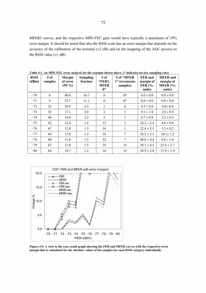
72

MFER5 curves, and the respective MPE-FEC gain would have typically a maximum of 10% error margin. It should be noted that also the RSSI scale has an error margin that depends on the accuracy of the calibration of the terminal (±2 dB) and on the mapping of the AGC process to the RSSI value (±1 dB).

Table 4-1. An MPE-FEC error analysis for the example shown above. (* indicates too low sampling rate). RSSI (dBm)

# of samples

Margin of error (95 %)

Sampling fraction

# of “FER1, MFER

0”

# of “MFER 1” (erroneous

samples)

FER and margin of FER (%-

units)

MFER and margin of

MFER (%-units)

�70 6 40.0 16.7 0 0* 0.0 ± 0.0 0.0 ± 0.0 �71 9 32.7 11.1 0 0* 0.0 ± 0.0 0.0 ± 0.0 �72 22 20.9 4.5 1 0 4.5 ± 0.9 0.0± 0.0 �73 33 17.1 3.0 2 1 9.1 ± 1.0 3.0 ± 0.5 �74 46 14.4 2.2 3 1 8.7 ± 0.9 2.2 ± 0.3 �75 62 12.4 1.6 12 3 24.2 ± 2.4 4.8 ± 0.6 �76 67 12.0 1.5 14 1 22.4 ± 2.5 1.5 ± 0.2 �77 69 11.8 1.4 18 7 36.2 ± 3.1 10.1± 1.2 �78 80 11.0 1.3 32 7 48.8 ± 4.4 8.8 ± 1.0 �79 67 12.0 1.5 25 15 59.7 ± 4.5 22.4 ± 2.7 �80 84 10.7 1.2 16 15 36.9 ± 2.0 17.9 ± 1.9

CDF, FER and MFER with error margins

0.0

5.0

10.0

15.0

20.0

-70 -71 -72 -73 -74 -75 -76 -77 -78 -79 -80RSSI (dBm)

Out

age-

%

FERMFERFER minFER maxMFER minMFER max

Figure 4-9. A view to the case result graph showing the FER and MFER curves with the respective error margin that is calculated for the absolute values of the samples for each RSSI category individually.

73

If the accuracy of the above mentioned measurement methodology should be enhanced, more samples would need to be collected per RSSI category. It is obvious that apart from the impulse noise environment which might produce errors in large RSSI window, a sufficiently good field strength provides with reliable results (non-erroneous samples) even with low amount of sam-ples, whereas erroneous frames are produced relatively often in the lowest field. If the investi-gation does not concentrate on the impulse noise, it is thus sufficient to collect the major part of the samples around the critical RSSI scale of the 5% breaking point of FER and MFER.

On the other hand, the idea of the above mentioned method is to collect fast snap-shot data which means that the task could be carried out in relatively short time period per investigated area. Typically, the storing of each measurement sample (frame) could take about 1 second, and assuming that in sufficiently accurate analysis ±5 RSSI values, i.e. about 11 RSSI categories need to be measured, e.g. with 300 samples per RSSI category producing margin of error of 5.7 %, this would require 11 ⋅ 300 ⋅ 1 s = 3300 s, i.e. 55 minutes would be needed. In typical meas-urement routines of an operator, this might be in the practical limit of the used work time for a single measurement, although the error margin would provide with a better accuracy.

According to the results, the analysis described in Publication II might produce relatively smooth FER and MFER curves, which results in a straightforward way of comparison of FER5 and MFER5 points and indicates thus the respective MPE-FEC gain with a relatively high con-fidence level. In some cases, though, the curve behaviour is more "aggressive", producing high peaks along the RSSI scale an making the FER5 and MFER5 interpretation challenging. A part of these peaks can be explained by impulse noise, and some can be occurring due to the lack of samples. Nevertheless, the most important RSSI scale is in the range corresponding the FER5 and MFER5, and normally the phenomena of the correction capability can be seen graphically even if the FER5 and MFER5 breaking points are not implicitly possible to interpret. One way of trying to get the approximate value for the breaking point in this type of cases would be to interpolate regression curves for the FER and MFER graphs. The error margin could be esti-mated by observing the difference between the regression curve and the original deviating points. Nevertheless, the method would not reflect totally the reality as the errors do occur in non-predictable way along the RSSI scale in these cases making the reception unstable. The deeper analysis has thus not been made for this type of results in this thesis.

4.6 Effect of SFN [Publications III, IV, X] The SFN functionality has advantages in the normal operation as it produces gain by combining the signal energy of the multipath propagated separate radio signals. Reference [Bmc09, p. 15], though, has concluded that as SFN gain is not persistent across all locations of the DVB-H net-work, it is not considered in the radio link budget. In the theoretical case, if the carrier level is considered useful only if the minimum functional level of the investigated parameter settings is

74

achieved, the SFN gain can be obtained only in the overlapping area with C/N complying with the minimum functional value. Nevertheless, the C/N values just below the functional limit combined with the C/N value of other signals below the functional limit might set the sum of these signals above the functional level which enhances the coverage area between the sites. The more carrier components (above the noise limit) there is present in a certain spot, the more probably the sum of the signals exceed the minimum required C/N limit.

4.6.1 Non-interfered network

Publications IV and X present a variation of the Monte-Carlo simulation method, which can be utilized for estimating the SFN gain as a function of the most relevant radio parameters. The method is based on the investigation of the gain that is achieved in the physical level. The simulations resolve the received power level distribution in a single cell case, which is com-pared to the combined signals that are produced by n site cells. As the simulations are carried out over the whole investigated area at once instead of individual simulations of the sub-regions formed by the raster of the area map, the method provides a fast yet sufficiently accurate esti-mate of the gain, i.e. about the increased probability to receive the signal correctly.

Although the developed method is different from the other theoretical studies found in [Sil06], [Bee98], [Cha06], [Dvb09], [Law01], and [Ung08], it can be compared with the results found in these references. The practical field test based references are, on the other hand, limited as they are typically based on only few sites [Ple08] [Ple09] [Ple09b] [Bov09]. The presented simula-tion method takes into account all the site cells that contribute either to the useful received car-rier power or to the received interfering power within their range of radio propagation.

In the non-interfering case, there are only useful carriers present. The basic principle of the SFN gain calculation is based on the summing of the received power levels [ ]kRX CP )( in absolute values (W) as shown in Formula:

[ ] [ ]( ) )()()()(1

WCPWCPn

kkRXtotRX �

=

= (4-5)

The principle of power summing has been presented in [Ebu05] and it has been used in the re-ceived power level estimations, e.g. in [Sil06]. In the annexed Publications, the received power level is observed originally in dBm. For the power summing, the absolute value is thus first ob-tained by:

[ ]1000

10)()(10

)(��

��

�

=

dBmP

RX

RX

WCP (4-6)

75

In order to compare the SFN gain value, the reference level of received power level, at given time and location, is the strongest possible from the sites that can be received above the noise floor:

[ ] [ ] [ ]{ }nRXRXRXRXref CPCPCPP )(,...,)(,)(max 21= (4-7)

Now, the SFN gain GSFN is the difference between the summed and reference levels in dBm val-ues:

[ ] [ ]��

��

⋅= −3101

)()(log10)()( WCPdBmCP RXRX (4-8)

[ ] [ ] )()()()()( dBmCPdBmCPdBG refRXtotRXSFN −= (4-9)

Publications III, IV, VII and X assumes that the whole OFDM channels, i.e. multi-propagated signals, can be summed without taking into account the frequency selectivity within each band-width. It is obvious that especially in case of Rayleigh fading, a part of the subcarriers of a sin-gle OFDM bandwidth experiences higher attenuation than the others.

As the overall effect is a combination of possibly some destroyed sub-channels via the Rayleigh fading, and corrected sub-channels via the error recovery properties of MPE-FEC, it can be es-timated that the significance of the frequency selectivity is low for the calculation of the SFN gain in the way that is presented in this thesis. The practical observations from the DVB-H trials support this reasoning [Tal10]. Furthermore, the C/N values that are utilized as criteria in the simulations of this thesis are based on the [Dvb09] which has included the radio channel be-haviour already in the presented C/I limits.

The principle of the general power level summing for the high-level simulation purposes is shown in Figure 4-10 which presents an example of three non-correlating individual signals with approximately the same average levels as a function of time and location. These data is derived from the individual measurements of a single site carried out in Publication III, and the represent a mix of channel types including the long-term and fast fading. These data are aver-aged by the terminal to the 1 second resolution, so the highest Rayleigh attenuation peaks can not be shown in this example.

Figure 4-10 presents also the sum of these signals by applying the SFN expression (4-5). As can be noted, the resulting signals, in addition to the increased total received power level, have smaller variations. Figure 4-11 shows the CDF of the individual and combined signal levels. Table 4-2 and

Table 4-3 summarise this behaviour by presenting the numerical values.

76

Individual signals

-85

-80

-75

-70

-65

Signal 1

Signal 2

Signal 3

Summed signals

-85

-80

-75

-70

-651

Sum (1-2)

Sum (1-3)

Figure 4-10. An example of individually received signal levels in the same area, and their total power based on the direct power summing. The same terminal was utilized.

CDF

0.0

0.1

0.2

0.3

0.4

0.5

0.6

0.7

0.8

0.9

1.0

-90

-88

-86

-84

-82

-80

-78

-76

-74

-72

-70

-68

-66

Signal 1, original

Signal 2, original

Signal 3, original

Signals 1-2, summed

Signals 1-3, summed

Figure 4-11. CDF of the 3 individual and summed signals presented in Figure 4-11.

Table 4-2. Numerical values of individual signals of the example.

Signal # Average RSSI (dBm) Stdev (dB) 50%-ile of CDF

(dBm)

1 �75.0 2.9 �75.5 2 �79.2 3.5 �79.5 3 �77.2 3.9 �77.2

77

Table 4-3. The values of the summed signals of the example. GSFN is calculated by comparing the average and 50%-ile level with the strongest individual signal of each case.

Summed signals Average RSSI (dBm) Stdev (dB) 50%-ile of CDF

(dBm) GSFN /

reference signal #

1, 2 �73.2 2.3 �74.2 +1.8 dB (averages) +1.3 dB (50%-iles)

Ref: Signal #1

1, 2, 3 �71.4 2.3 �72.2 +3.6 dB (averages) +3.3 dB (50%-iles)

Ref: Signal #1

The above presented example shows the principle of the summing of power levels. The same principle is applied in the simulator presented in Annex 1. There are also analytical methods developed for the fast fading signal combining as presented in [Fus08], and SFN coverage prob-ability estimation as presented in [Lig99b] and [Lig99c]. Nevertheless, this thesis uses the power summing of the carriers and interfering components only via Monte-Carlo simulations.

The non-interfered case of the simulation results presented in IV can be used for the SFN gain estimations. The suitable principle is based on the filtered coverage area of a single cell, which gives the reference for the cumulative C/N. Then, more cells are added according to the SFN reuse pattern size presented in Figure 3 of Publication IV, and the C/N distribution is simulated for each case. The GSFN can be obtained by comparing the 10 % outage probability level (which corresponds to a 90 % area location probability within the whole area) of the CDF of each case.

Figure 4-12. An example of the simulated area with the SFN reuse pattern size K=7.

Table 4-4 presents comparisons of the SFN gain studies presented in the references that were found by the writing of this thesis.

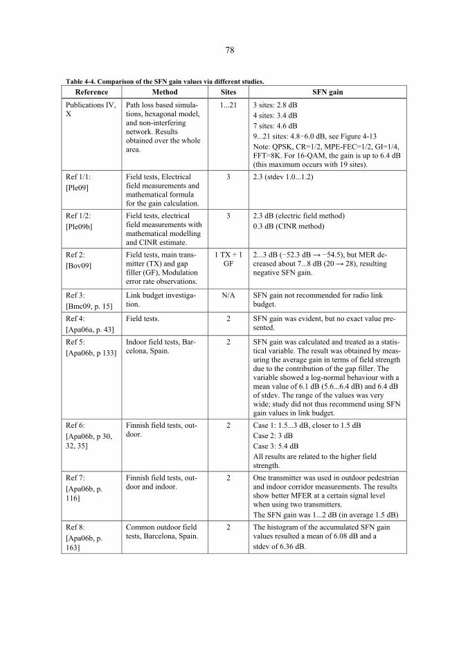
78

Table 4-4. Comparison of the SFN gain values via different studies. Reference Method Sites SFN gain

Publications IV, X

Path loss based simula-tions, hexagonal model, and non-interfering network. Results obtained over the whole area.

1...21 3 sites: 2.8 dB 4 sites: 3.4 dB 7 sites: 4.6 dB 9...21 sites: 4.8�6.0 dB, see Figure 4-13 Note: QPSK, CR=1/2, MPE-FEC=1/2, GI=1/4, FFT=8K. For 16-QAM, the gain is up to 6.4 dB (this maximum occurs with 19 sites).

Ref 1/1: [Ple09]

Field tests, Electrical field measurements and mathematical formula for the gain calculation.

3 2.3 (stdev 1.0...1.2)

Ref 1/2: [Ple09b]

Field tests, electrical field measurements with mathematical modelling and CINR estimate.

3 2.3 dB (electric field method) 0.3 dB (CINR method)

Ref 2: [Bov09]

Field tests, main trans-mitter (TX) and gap filler (GF), Modulation error rate observations.

1 TX + 1 GF

2...3 dB (�52.3 dB �54.5), but MER de-creased about 7...8 dB (20 28), resulting negative SFN gain.

Ref 3: [Bmc09, p. 15]

Link budget investiga-tion.

N/A SFN gain not recommended for radio link budget.

Ref 4: [Apa06a, p. 43]

Field tests. 2 SFN gain was evident, but no exact value pre-sented.

Ref 5: [Apa06b, p 133]

Indoor field tests, Bar-celona, Spain.

2 SFN gain was calculated and treated as a statis-tical variable. The result was obtained by meas-uring the average gain in terms of field strength due to the contribution of the gap filler. The variable showed a log-normal behaviour with a mean value of 6.1 dB (5.6...6.4 dB) and 6.4 dB of stdev. The range of the values was very wide; study did not thus recommend using SFN gain values in link budget.

Ref 6: [Apa06b, p 30, 32, 35]

Finnish field tests, out-door.

2 Case 1: 1.5...3 dB, closer to 1.5 dB Case 2: 3 dB Case 3: 5.4 dB All results are related to the higher field strength.

Ref 7: [Apa06b, p. 116]

Finnish field tests, out-door and indoor.

2 One transmitter was used in outdoor pedestrian and indoor corridor measurements. The results show better MFER at a certain signal level when using two transmitters. The SFN gain was 1...2 dB (in average 1.5 dB)

Ref 8: [Apa06b, p. 163]

Common outdoor field tests, Barcelona, Spain.

2 The histogram of the accumulated SFN gain values resulted a mean of 6.08 dB and a stdev of 6.36 dB.

79

According to Table 4-4, the SFN gain value varies largely even with a low number of transmit-ters (2–3), the minimum gain being 1...1.5 dB and maximum being over 6 dB, depending on the source. The gain obtained from Publications IV and X represents a typical average value range of the other sources thus correlating with major part of the presented references when the num-ber of sites is up to 3.

Unlike the other presented results, [Bov09] has concluded that the SFN gain would actually be negative in a two-transmitter case due to the significant degradation of the signal quality meas-ured by the modulation error rate (MER) indicator. This outcome clearly differs from the other references. The source does not present the cause for the effect, but the explanation might be that the presented test setup includes some feedback loop interferences between the input and output of the gap filler.

The reference [Mil06, p. 71] shows that as the gain margin of the gap filler gets close to zero the ripple increases considerably. At 0 dB gain margin point the system is already unstable. As the gap filler setup is critical in the SFN analysis, the most reliable results might be derived from the test cases where only main transmitters are switched on and off as explained in [Ble08] and [Ble09].

As an overall observation, the field tests that are related to the SFN gain have normally been carried out with only two transmitters. In [Ble08], a method of adding the electrical field strengths from a total of three main transmitters resulted in a total SFN gain of 2.3 dB. Never-theless, in a further analysis related to the same network, [Ble09] has found that the CINR re-sults in only 0.3 dB gain. This indicates that SFN gain should be estimated case-by-case by in-vestigating what is the effect of the interference level, e.g. for the MER degradation, not only the sum of electrical field strength.

Figure 4-13 shows a summary of the SFN gain results obtained via the simulations of Publica-tion IV, Figure 12. The originally presented non-uniform SFN reuse pattern size scale has been converted linear and a logarithmic regression curve has been added to the resulting plots. The reference results from Table 4-4 have also been marked in the graph for comparison purposes. As can be observed, the SFN gain values of the found references vary considerably. The main reason for this can probably be explained by the differences in the practical setup, which might not be described in a sufficiently detailed level in the references in order to understand, what the size of the coverage area of a single site is compared to the coverage are produced by the gap-filler or secondary transmitter.

Although the results of Publications IV and X are based on simulations, the setup was made in a controlled way by selecting the overlapping proportions of the site cells according to the hex-agonal layout model, i.e. there were sufficiently overlapping parts present but without excess. The results are derived always from the filtered cell areas, i.e. within the dimensioned cell based

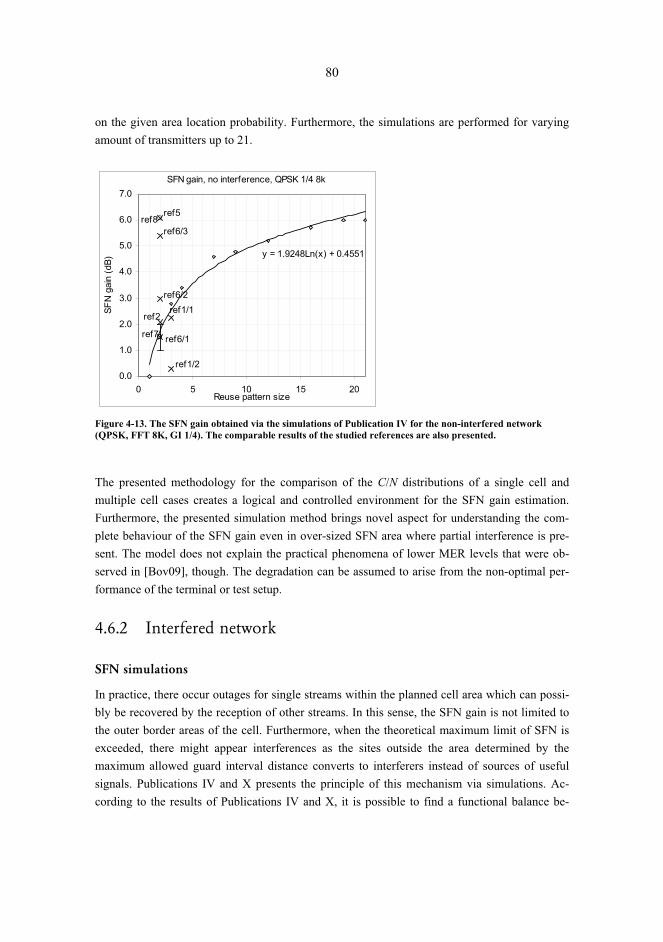
80

on the given area location probability. Furthermore, the simulations are performed for varying amount of transmitters up to 21.

SFN gain, no interference, QPSK 1/4 8k

ref1/1ref2

ref1/2

ref5

ref6/1

ref6/2

ref6/3

ref7

ref8

y = 1.9248Ln(x) + 0.4551

0.0

1.0

2.0

3.0

4.0

5.0

6.0

7.0

0 5 10 15 20Reuse pattern size

SFN

gai

n (d

B)

Figure 4-13. The SFN gain obtained via the simulations of Publication IV for the non-interfered network (QPSK, FFT 8K, GI 1/4). The comparable results of the studied references are also presented.

The presented methodology for the comparison of the C/N distributions of a single cell and multiple cell cases creates a logical and controlled environment for the SFN gain estimation. Furthermore, the presented simulation method brings novel aspect for understanding the com-plete behaviour of the SFN gain even in over-sized SFN area where partial interference is pre-sent. The model does not explain the practical phenomena of lower MER levels that were ob-served in [Bov09], though. The degradation can be assumed to arise from the non-optimal per-formance of the terminal or test setup.

4.6.2 Interfered network

SFN simulations

In practice, there occur outages for single streams within the planned cell area which can possi-bly be recovered by the reception of other streams. In this sense, the SFN gain is not limited to the outer border areas of the cell. Furthermore, when the theoretical maximum limit of SFN is exceeded, there might appear interferences as the sites outside the area determined by the maximum allowed guard interval distance converts to interferers instead of sources of useful signals. Publications IV and X presents the principle of this mechanism via simulations. Ac-cording to the results of Publications IV and X, it is possible to find a functional balance be-

81

tween the raised interference level and the compensating SFN gain even in the over-sized SFN network.

The simulation method presented in Publication IV takes into account the SFN gain in interfered DVB-H networks, i.e. when the parameters affecting on the SFN size are selected in such a way that there are sites found outside the theoretical SFN area (as shown in Table 2-1).

The level of the interference can first be investigated in a general level by observing the interfered links between the sites that are exceeding the SFN limits. When the number of these potential interference sources is compared with the total number of links between all the sites, the severity of the interference in the investigated area can be noted. As can be observed from Tables 3 and 4 of Publication IV, there exists parameter sets which result in interference levels up to 100 %. The higher the amount of the potential interfering links is, the more probable the network experiences quality degradation.

There is also a set of parameters that results only partial interference levels. As shown in Figure 6 of Publication X, the interference level is not constant, though, but tends to be switched on and off depending on the location of the terminal in the field. This is due to the fact that the dif-ference between the arriving signals is the one that determinates weather the signal is interfered or not.

When all the sites are within the SFN area, i.e. when the distance between of any of the sites is equal or less than the theoretical maximum SFN diameter distance DSFN, there will be no inter-ferences. This is the case also if the receiver is located outside the circle defined by DSFN. This can be shown by investigating the distance between the receiver and the dominating site com-pared to the distance of the receiver and any of the other sites. The difference between these distances defines the effective distance Deff of the signal. This distance can be investigated by making the receiver drift away of the SFN circle towards any direction as presented in Figure 4-14. The absence of the interferences can be investigated by observing the angle β of Figure 4-14. It can be seen that Deff is maximum when cos β = 1. In that case, Deff = DSFN, i.e. Deff never exceeds DSFN when no sites are located outside of the SFN area.

When the distance between any of the two sites using the same frequency is longer than the DSFN, there will be interferences in the locations where the Deff > DSFN. The interference distri-bution can be observed by defining two sites in the simulator that was used in Publications III, IV and VII. By selecting a parameter set of GI=1/4 and FFT = 2K, the DSFN would be 16.8 km. The simulation of two sites in a 45 × 45 km2 area, with x/y-coordinates of (14.9, 22.5) and (30.1, 22.5) shows that there are no interferences present at any point as the inter-site distance is at the maximum allowed value of 16.8 km. The site antenna height was then set to 80 m, EIRP to +70 dBm, and the first site was moved to the coordinate (10.0, 22.5), i.e. the inter-site distance was extended to 20.1 km. The standard deviation of the long-term fading was maintained in 5.5 dB

82

and the area location probability as 70 %. When the maximum DSFN is exceeded by 4.9 km, the interference is present in areas where Deff > DSFN as can be seen via the simulation result shown in Figure 4-15.

Delay 1

Delay 2

Max SFN diameter = DSFN

SFN area

TX1 TX2

β

Delay 1

Delay 2

Max SFN diameter = DSFN

SFN area

TX1 TX2

β

Figure 4-14. There are no interferences when the sites are within the SFN area even if the receiver drifts out-side of the SFN area. The reception within this outer zone is thus possible whenever the minimum required C/N can still be reached.

Figure 4-15. When the distance of two sites exceed the SFN limit, there occur interferences in those areas where Deff > DSFN. Figure shows the interference zone that applies for Deff > DSFN everywhere with the I-component greater than the noise floor. In this case, PTX is +70 dBm and the site antenna height is 80 m. The total area size is 45 km × 45 km.

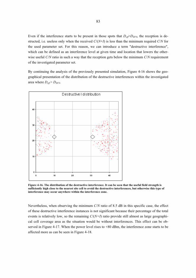
83

Even if the interference starts to be present in those spots that Deff>DSFN, the reception is de-structed, i.e. useless only when the received C/(N+I) is less than the minimum required C/N for the used parameter set. For this reason, we can introduce a term "destructive interference", which can be defined as an interference level at given time and location that lowers the other-wise useful C/N ratio in such a way that the reception gets below the minimum C/N requirement of the investigated parameter set.

By continuing the analysis of the previously presented simulation, Figure 4-16 shows the geo-graphical presentation of the distribution of the destructive interferences within the investigated area where Deff > DSFN.

Figure 4-16. The distribution of the destructive interference. It can be seen that the useful field strength is sufficiently high close to the nearest site cell to avoid the destructive interferences, but otherwise this type of interference may occur anywhere within the interference zone.

Nevertheless, when observing the minimum C/N ratio of 8.5 dB in this specific case, the effect of these destructive interference instances is not significant because their percentage of the total events is relatively low, so the remaining C/(N+I) ratio provide still almost as large geographi-cal cell coverage area as the situation would be without interferences. This effect can be ob-served in Figure 4-17. When the power level rises to +80 dBm, the interference zone starts to be affected more as can be seen in Figure 4-18.

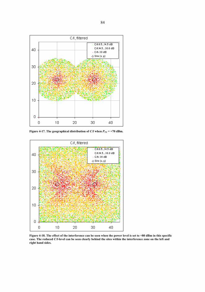
84

Figure 4-17. The geographical distribution of C/I when PTX = +70 dBm.

Figure 4-18. The effect of the interference can be seen when the power level is set to +80 dBm in this specific case. The reduced C/I-level can be seen clearly behind the sites within the interference zone on the left and right hand sides.

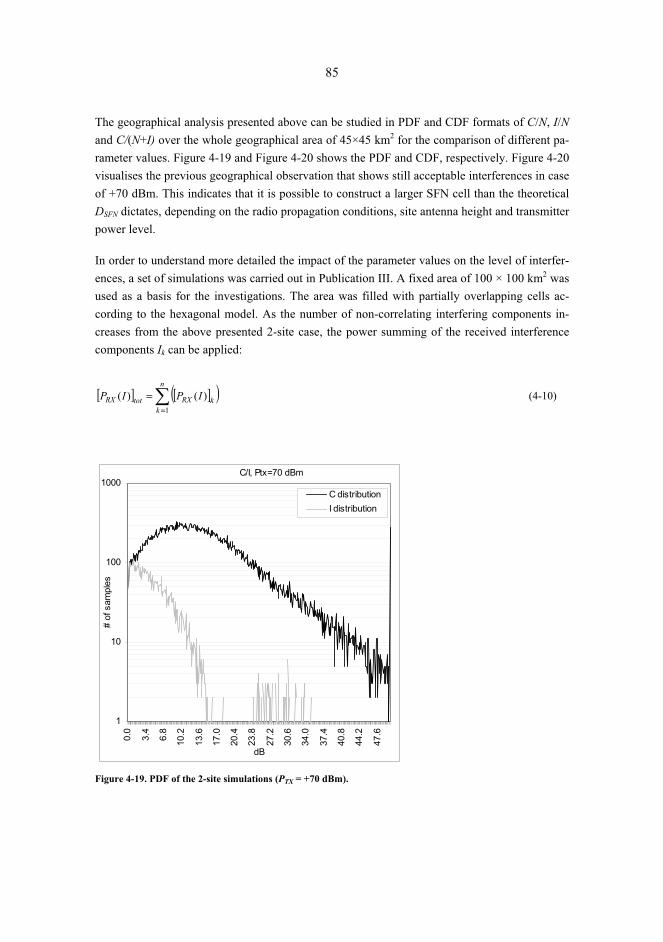
85

The geographical analysis presented above can be studied in PDF and CDF formats of C/N, I/N and C/(N+I) over the whole geographical area of 45×45 km2 for the comparison of different pa-rameter values. Figure 4-19 and Figure 4-20 shows the PDF and CDF, respectively. Figure 4-20 visualises the previous geographical observation that shows still acceptable interferences in case of +70 dBm. This indicates that it is possible to construct a larger SFN cell than the theoretical DSFN dictates, depending on the radio propagation conditions, site antenna height and transmitter power level.

In order to understand more detailed the impact of the parameter values on the level of interfer-ences, a set of simulations was carried out in Publication III. A fixed area of 100 × 100 km2 was used as a basis for the investigations. The area was filled with partially overlapping cells ac-cording to the hexagonal model. As the number of non-correlating interfering components in-creases from the above presented 2-site case, the power summing of the received interference components Ik can be applied:

[ ] [ ]( )�=

=n

kkRXtotRX IPIP

1

)()( (4-10)

C/I, Ptx=70 dBm

1

10

100

1000

0.0

3.4

6.8

10.2

13.6

17.0

20.4

23.8

27.2

30.6

34.0

37.4

40.8

44.2

47.6

dB

# of

sam

ples

C distributionI distribution

Figure 4-19. PDF of the 2-site simulations (PTX = +70 dBm).

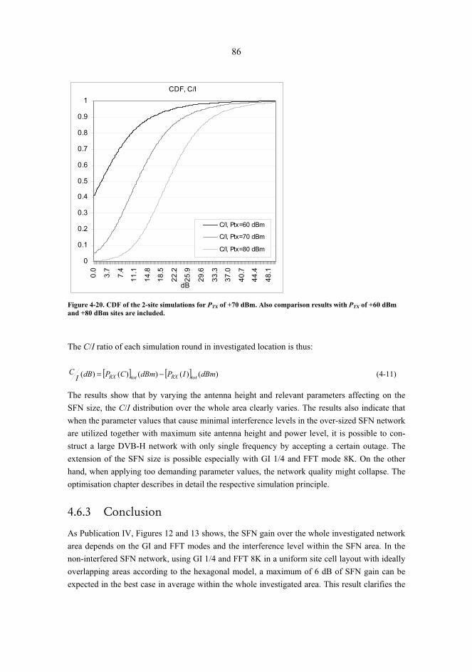
86

CDF, C/I

0

0.1

0.2

0.3

0.4

0.5

0.6

0.7

0.8

0.9

10.

0

3.7

7.4

11.1

14.8

18.5

22.2

25.9

29.6

33.3

37.0

40.7

44.4

48.1

dB

C/I, Ptx=60 dBm

C/I, Ptx=70 dBm

C/I, Ptx=80 dBm

Figure 4-20. CDF of the 2-site simulations for PTX of +70 dBm. Also comparison results with PTX of +60 dBm and +80 dBm sites are included.

The C/I ratio of each simulation round in investigated location is thus:

[ ] [ ] )()()()()( dBmIPdBmCPdBIC

totRXtotRX −= (4-11)

The results show that by varying the antenna height and relevant parameters affecting on the SFN size, the C/I distribution over the whole area clearly varies. The results also indicate that when the parameter values that cause minimal interference levels in the over-sized SFN network are utilized together with maximum site antenna height and power level, it is possible to con-struct a large DVB-H network with only single frequency by accepting a certain outage. The extension of the SFN size is possible especially with GI 1/4 and FFT mode 8K. On the other hand, when applying too demanding parameter values, the network quality might collapse. The optimisation chapter describes in detail the respective simulation principle.

4.6.3 Conclusion

As Publication IV, Figures 12 and 13 shows, the SFN gain over the whole investigated network area depends on the GI and FFT modes and the interference level within the SFN area. In the non-interfered SFN network, using GI 1/4 and FFT 8K in a uniform site cell layout with ideally overlapping areas according to the hexagonal model, a maximum of 6 dB of SFN gain can be expected in the best case in average within the whole investigated area. This result clarifies the

87

SFN gain behaviour. It can thus be assumed that this result is more realistic than the information of [Bmc09, p. 15] that recommends the use of 0 dB as SFN gain value in DVB-H radio link budget.

On the other hand, the definition of [Bmc09] is not very accurate. Instead, it informs that SFN gain is “the reduction of number of transmitters to cover a given area using synchronised trans-mitters compared to the number of independent MFN transmitters”. [Bmc09] concludes that “depending on the network topology, this transmitter savings may be carefully translated into an average increase of coverage. However, the SFN gain is not persistent across all points of the network, so it will not be considered in the link budget.” It can be interpreted that this definition assumes that the benefit of SFN could be obtained basically in the site cell edges and that the overall gain is challenging to estimate. Publication IV shows, though, that the total gain is pos-sible to estimate over the whole investigated area to be utilized as a generalized radio link budget value.

Based on the simulations of Publication IV, SFN gain of 0�6 dB could be applied to the DVB-H radio link budget depending on the parameter settings and the total number of the transmitter sites per SFN area. For the local adjustments of the SFN value of the link budget, a respective simulation method can be applied by varying the GI, FFT, code rate, power level and antenna height settings. In a realistic network, the SFN gain could be taken into account when the site locations and other parameters are selected. The SFN gain can be simulated over the planned area, and its effect can be taken into account both in non-interfered and over-sized SFN cell by reducing the transmitter power levels and/or lowering the assumption of the antenna height, which gives more freedom in the optimal deployment if there are problems in using the values for the power or antenna height that the original plan indicates. If the SFN gain can be simulated in early phase of the first deployment plan, it can influence on the optimal site selections.

As an outcome of the SFN gain related simulations presented in this thesis, the definition of the SFN gain has been clarified. The method takes into account the combination of the gain and interference within the whole investigated network, not only non-interfered environment and in limited locations as the other found publications typically show. The case dependent SFN gain value could thus be investigated by applying the proposed simulation method.

4.7 Radiation limitations [Publication VI] The installation of the DVB-H sites must comply with the local and international regulations of the EMC limits and the safety zones related to the limitations of exposure of the public to non-ionizing radiation of the signals. On the other hand, the installation of DVB-H antennas should be designed in such a way that the other systems located nearby will not cause interferences to the DVB-H transmission, and vice versa.

88

The general limitations of exposure should be investigated via the national and international regulations. European Union dictates the limits for the member countries. As an example, the regulation in Finland covers the frequency band 0�300 GHz [Reg02]. The format and values of the limits varies though depending on the regulator. As another example, FCC informs the limitations for cellular and broadcast environment in USA as a function of the antenna height and installation type as indicated in [Fcc98] and [Fcc07]. The allowed limit in 700 MHz band is maximally 50 kW ERP, but decreases when the antenna height is lower.

When initiating the planning process, the general maximum power limit should be taken into account. When the plan advances, also the EMC and safety zones should be estimated as accu-rately as the planning phase allows. When the final plan is under work, the site specific safety zones should be estimated.

Publication VI describes the principles for the dimensioning of the radiation levels and how the safety zone can be taken into account in rooftop and tower installations of DVB-H. The calcula-tions are based on the formulas shown in [Min99]. The respective level should also be taken into account in the CAPEX/OPEX optimisation as the maximum allowed power level may change the optimal transmitter power depending on the case.

Publication VI shows case examples about the estimation of the levels in a typical DVB-H an-tenna installation setup. In a standard scenario, the DVB-H site consists of directional antennas either in towers or rooftops. The radiation pattern should be taken into account accordingly in vertical and horizontal layers. The radiation safety distance calculations should be carried out for different sides of the antenna. Publication VI proposes a method that takes into account the radiation in back lobe by estimating a maximum value over the complete half of the hemisphere. For the field below the antenna, the estimation can be made based on the vector's angle in verti-cal plane and respective amplitude that depends on the vertical radiation pattern of the antenna. This method is relatively simple but functional in the typical DVB-H deployment. The method was not found in this specific format in the related references [Chu00] [Fcc98] [Min99] [Reg02] [Sci07].

As a summary, the regulatory limits dictates the maximum radiating power PTX,reg and EMC / radiation safety analysis results in the maximum radiating power in site-basis PTX,safety, the opti-mal radiating power PTX,opt that is obtained via the CAPEX / OPEX optimisation can thus move based on the formula:

{ }safetyTXregTXoptTXTX PPPP ,,, ,,min= (4-12)

The selection of the final radiating power level PTX, might thus require changes of either the an-tenna heights, transmitter power levels or both, reducing the site cell coverage. The respective analysis should be taken into account in general level in the nominal radio network planning

89

(the correct selection of the uniform power levels) and in the detailed radio network planning (by applying the analysis in individual site basis). The final selection of PTX might also require various iteration rounds in order to find the optimal point of technical and economical parame-ters.

It should be noted that the radiation analysis method presented in Publication VI utilizes direc-tional antennas as a basis for the examples. Nevertheless, only omni-radiating antennas were utilized in the SFN simulations described in Publications III and IV. The selection of the omni-directional antennas in the simulations is due to the practical point of view that the DVB-H site cell is typically done as omni-directional, either by utilizing the omni-radiating antenna (pole), or a set of directional antennas in order to create the omni-radiating coverage. The utilization of the directional antennas in the simulations has been noted as a potential future study, with the analysis of the effect of the antenna down-tilt on the radio performance (for maximizing the SFN gain and minimizing the SFN interference level).

The directional antenna has been studied in the radiation related publication because this pro-vides a practical methodology and useful examples of the expected outcome for the installation of the antenna elements, with safety distance estimations below and on the sides of the antennas. The outcome gives a realistic estimation of the radiation for the antenna installations in roof-tops, in roof edge parts, where the omni-directional element would not be a logical solution. Nevertheless, the method is valid also for the omni-radiating elements.

4.8 Cost prediction [Publication I] In the complete network planning, the cost effect needs to be taken into account in every phase. In the initial phase of the network planning, a rough estimation of the average site cost as well as the total cost of the area of interest is sufficient. The total channel capacity requirement de-pends on the number of the channels and their respective quality level. The demand for the ser-vices and thus additional capacity can be expected to grow as a function of time as stated in [Ski06, p.2].

The detailed plan should already contain more in-depth analysis of the network costs as for the CAPEX and OPEX. In this phase, it is possible to take into account different solutions, includ-ing the transmitter type, transmission, preferable and available antenna heights, antenna types, site solutions in general etc. It is important to balance the costs with the technical solutions, i.e. the hardware, software and related technical quality, coverage and capacity of the network. The cost effect is such an important item that it should be taken into account preferable in an itera-tive way, i.e. in order to seek the optimal point of technical and commercial balance, possibly several planning scenarios should be carried out. The more detailed cost optimisation is ex-plained in Chapter 5.3.

90

It can be assumed that uniform parameter values may be applied for the site costs in the initial planning, because the final site locations or site specific radio parameters are not necessarily confirmed yet. In the later phase, during the detailed planning, site-specific assumptions should be utilized instead for the more in-depth cost optimisation.

In this thesis, the case examples of the DVB-H deployment and operation cost optimization are studied by using the hexagonal network layout. In practice, the sites do have variable antenna heights and power levels as well as non-uniform locations. The presented case examples are shown for the uniform comparison in order to select the most feasible parameter combination from the relative analysis, but the methodology can be applied also in the real environment with site specific parameter values. In that case, the model should be applied by selecting the already existing sites – that can be from both broadcast and mobile networks – and by identifying a set of additional site candidates with a "best effort" assumption for their probable, individual pa-rameter values. As the site locations are fixed in that case in a non-uniform way, the coverage analysis should be carried out by adjusting the power levels, antenna heights, and respective costs of each site separately iteratively way until each case produces the wanted coverage qual-ity level. This thesis does not consider the non-uniform cases, though.

91

5 Optimisation

5.1 Site parameters

5.1.1 Controlled SFN interference [Publications III, X]

In some cases, there might be a need to extend the maximum theoretical SFN by building more sites in wider areas than the guard interval allows in theory. This might be relevant, e.g. in a very large city with a single network topology. The division of the area could be made by se-lecting two or more frequencies for MFN and creating separate SFN isles. The handover be-tween the isles provide a fluent continuum of the service. Nevertheless, e.g. the lack of available frequencies might require the use of an extended SFN.

Publication III presents a method for the simulations of the over-sized SFN area, including case results that indicate how the C/(N+I) ratio behaves over the whole investigated area. The simu-lations are based on the hexagonal model, and the idea is to select a rectangular area with x- and y-coordinates which is filled in with partially overlapping cells. A set of parameters was studied by varying the modulation scheme, FFT and antenna height of all the sites, i.e. a uniform net-work was considered in each simulation case. The radius of the cells was calculated in the initial phase of each simulation in order to create a perfectly dimensioned radio network. The C/(N+I) ratio of 8.5 dB was utilised as a limit for QPSK, and 14.5 dB for 16-QAM. The radiating power level of the sites was maintained constantly in +60 dBm. The GI was fixed to 1/4, CR to 1/2 and MPE-FEC rate to 1/2. The studied area was 100 × 100 km2 for each case, i.e. depending of the antenna height and modulation, the total amount of the site cells varied according to the cell ra-dius.

The power summing for the useful carriers as well as for the interfering signals was applied in the simulations as indicated in [Ebu05, p. 55]. The developed simulator is based in the Monte-Carlo method. As a difference for the typical area element based coverage study mentioned in [Ebu05, p. 55] and [Gom09, p. 86], the percentage of the useful signal levels was simulated over the complete area without sub-area division. This is because the coverage area as such was not investigated visually, but the relative difference of the CDF of C/(N+I) was solved for the in-vestigated parameter values. It can be estimated that this method gives an accurate result for this purpose in much faster time frame compared to the separate simulations of each sub-area.

Figure 5-1 shows the outcome of the simulations for the QPSK and 16-QAM modulation schemes. Each plot represents an individual simulation of 60,001 snap-shot rounds. Figure 5-1

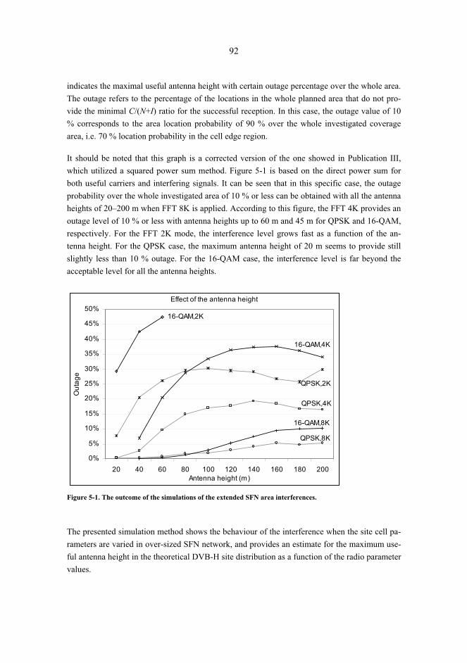
92

indicates the maximal useful antenna height with certain outage percentage over the whole area. The outage refers to the percentage of the locations in the whole planned area that do not pro-vide the minimal C/(N+I) ratio for the successful reception. In this case, the outage value of 10 % corresponds to the area location probability of 90 % over the whole investigated coverage area, i.e. 70 % location probability in the cell edge region.

It should be noted that this graph is a corrected version of the one showed in Publication III, which utilized a squared power sum method. Figure 5-1 is based on the direct power sum for both useful carriers and interfering signals. It can be seen that in this specific case, the outage probability over the whole investigated area of 10 % or less can be obtained with all the antenna heights of 20–200 m when FFT 8K is applied. According to this figure, the FFT 4K provides an outage level of 10 % or less with antenna heights up to 60 m and 45 m for QPSK and 16-QAM, respectively. For the FFT 2K mode, the interference level grows fast as a function of the an-tenna height. For the QPSK case, the maximum antenna height of 20 m seems to provide still slightly less than 10 % outage. For the 16-QAM case, the interference level is far beyond the acceptable level for all the antenna heights.

Effect of the antenna height

QPSK,8K

QPSK,4K

QPSK,2K

16-QAM,8K

16-QAM,4K

16-QAM,2K

0%

5%

10%

15%

20%

25%

30%

35%

40%

45%

50%

20 40 60 80 100 120 140 160 180 200Antenna height (m)

Out

age

Figure 5-1. The outcome of the simulations of the extended SFN area interferences.

The presented simulation method shows the behaviour of the interference when the site cell pa-rameters are varied in over-sized SFN network, and provides an estimate for the maximum use-ful antenna height in the theoretical DVB-H site distribution as a function of the radio parameter values.

93

The simulation result of Figure 5-1 is interesting as it indicates that the DVB-H network can be build by exceeding the theoretical SFN size if QPSK or 16-QAM and {FFT=8K, GI=1/4} are utilized together with all the antenna heights of at least up to 200 m. Furthermore, {FFT=8K, GI=1/4} provides a functional QPSK or 16-QAM network for the typical mobile network sys-tems antenna heights.

By writing this thesis, only limited information about the over-sized SFN especially in DVB-H was found. Based on [Lig99c], the self-interference can be coped with in a large SFN. Also ref-erence [Ebu09] mentions the possibility to utilize nation-wide SFN deployment for the DVB-T, if the synchronization of the sites is planned. It also mentions that "For DVB-T, only the most rugged system variants allow for a national extension of the SFN coverage area (for larger coun-tries). These rugged system variants, however, provide only restricted data capacity (typically, 5 – 6 Mbit/s). For more practical system variants, with a data capacity between 13 and 24 Mbit/s, the size of the SFN coverage area is restricted to a diameter of 150 – 250 km."

Reference [Ebu05] shows an example about the effect of the slightly over-sized SFN by investi-gating the complete area location probability distribution in a geographical format. A fixed an-tenna height of 150 m, GI of 1/4 and FFT of 8K were selected for the study. The study mentions that the inter-transmitter distance in an SFN should not exceed by too much the distance equivalent to the guard interval length. The result shows the minimum coverage probability for DVB-T as a function of the transmitter power. It was concluded that the coverage probability did not fall below the designed value of 95% in any part of the network regardless of the over-sized SFN. It should be noted that the study was made for a relatively small amount of sites (7), and the setup was terrestrial digital television system specific.

The information about the more specific effect of the transmitter antenna height on the quality and utilization of the SFN especially in a typical DVB-H environment was still missing from the found references. Even the simulations presented in this thesis are based on a fixed DVB-H transmitter power, the results in anyway align with the observation of [Ebu09] about the useful-ness of the most robust variants of the DVB-T that works as a nationwide solution, i.e. in an over-sized SFN. Publication III confirms thus the possibility to extend the SFN by having in-vestigated a large amount of the DVB-H sites with a typical DVB-H transmitter power range that can be assumed to be between the power levels typically utilized in the DVB-T and mobile communications, and shows additional examples about the impact of the antenna installation in the DVB-H specific environment.

5.1.2 SFN gain and interferences [Publications IV, VII, X]

In addition to the interferences in the over-dimensioned SFN, there are also overlapping carriers producing SFN gain. Publications IV and X indicate that the balancing of the SFN interferences

94

and SFN gain can be done in controlled way. The presented studies show a methodology to simulate the quality level of the over-sized SFN by using theoretical hexagonal model as well as practical site locations.

The modelling of the radio interface was done by applying the long term and fast fading profiles in snap-shot simulation rounds. The simulation was repeated 60,001 times in order to achieve statistical reliability. It should be noted that for the simulations that used Rayleigh fading (that is applied only in Publication VII), the modelling of the fading was simplified and considered over the whole OFDM channel per simulation round. In the more detailed simulation, the attenuation peaks of the Rayleigh fading should affect only on part of the OFDM subcarriers. As this inves-tigation was done in higher level, and due to the practical limitations of the simulator, the sub-carrier specific behaviour was not considered and flat fading was applied even if the channel is frequency selective. This is justified as [Dvb09] considers the respective performance limits as a function of the overall C/N values. In other words, the fast fading can be assumed to be mini-mised at the physical layer with FEC and interleaving. Nevertheless, the more in-depth model-ling of the fast fading in wide-band DVB-H signal can be noted as a further study item.

In case of a non-interfered network, i.e. when the SFN area is dimensioned in such a way that the common distance of the sites never exceeds the maximum SFN limit, the SFN gain can be estimated by simulating and observing the cumulative presentation of the sum of the carrier power. If the SFN limit is exceeded, part of the sites starts acting as interfering sources. Simula-tions were carried out in this thesis in order to investigate the behaviour of the balance of the SFN gain of the useful carriers, and the negative SFN gain that the interferers cause.

Figure 5-2 shows an example of the balance that can be obtained with QPSK and the investi-gated radio parameter values presented in Publication IV (Figure 12). Publication IV estimated the maximum SFN gain in a slightly more pessimistic way due to the difference in the power summing whilst Figure 5-2 presents the outcome of the direct power summing.

The analysis shows that when the radio parameter values presented in Publication IV are util-ized, the parameter set of {QPSK, GI=1/4 and FFT=8K or 4K} produces an interference-free network for 1...21 sites. In this analysis, the sites are located according to the hexagonal network layout and are overlapping ideally. It can be seen from the figure that as the amount of the sites grows, the SFN gain (sum of the received power levels compared to a single site) reaches the saturation point which in this case is about 6.0 dB. The observation has been done inside the calculated site cell areas, by using a limit of the radius of the site cell that complies with the de-signing value of 10% outage probability in the site cell area. The parameter set of {QPSK, GI=1/4, FFT=2K} is still capable of producing SFN gain of about 3 dB in a large SFN, even the interference starts taking place after K=7 is exceeded. The parameter set of {QPSK, GI=1/8, FFT=2K} produces SFN gain in a small SFN, but the gain starts decreasing when K grows. With K value between 9 and 12, the SFN gain is 0 dB.

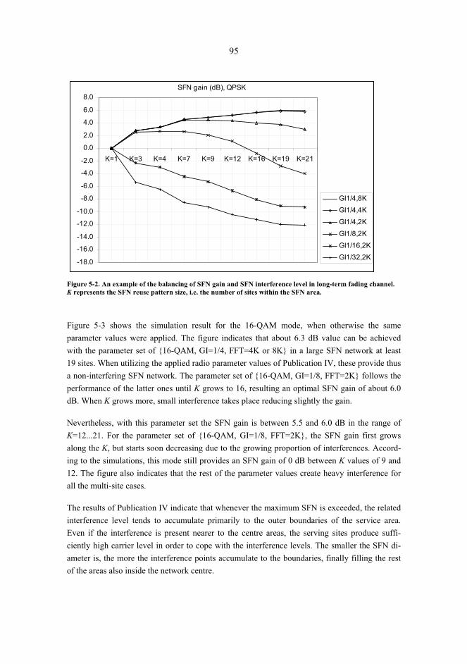
95

SFN gain (dB), QPSK

-18.0

-16.0

-14.0

-12.0

-10.0

-8.0

-6.0

-4.0

-2.0

0.0

2.0

4.0

6.0

8.0

K=1 K=3 K=4 K=7 K=9 K=12 K=16 K=19 K=21

GI1/4,8K

GI1/4,4K

GI1/4,2K

GI1/8,2K

GI1/16,2K

GI1/32,2K

Figure 5-2. An example of the balancing of SFN gain and SFN interference level in long-term fading channel. K represents the SFN reuse pattern size, i.e. the number of sites within the SFN area.

Figure 5-3 shows the simulation result for the 16-QAM mode, when otherwise the same parameter values were applied. The figure indicates that about 6.3 dB value can be achieved with the parameter set of {16-QAM, GI=1/4, FFT=4K or 8K} in a large SFN network at least 19 sites. When utilizing the applied radio parameter values of Publication IV, these provide thus a non-interfering SFN network. The parameter set of {16-QAM, GI=1/8, FFT=2K} follows the performance of the latter ones until K grows to 16, resulting an optimal SFN gain of about 6.0 dB. When K grows more, small interference takes place reducing slightly the gain.

Nevertheless, with this parameter set the SFN gain is between 5.5 and 6.0 dB in the range of K=12...21. For the parameter set of {16-QAM, GI=1/8, FFT=2K}, the SFN gain first grows along the K, but starts soon decreasing due to the growing proportion of interferences. Accord-ing to the simulations, this mode still provides an SFN gain of 0 dB between K values of 9 and 12. The figure also indicates that the rest of the parameter values create heavy interference for all the multi-site cases.

The results of Publication IV indicate that whenever the maximum SFN is exceeded, the related interference level tends to accumulate primarily to the outer boundaries of the service area. Even if the interference is present nearer to the centre areas, the serving sites produce suffi-ciently high carrier level in order to cope with the interference levels. The smaller the SFN di-ameter is, the more the interference points accumulate to the boundaries, finally filling the rest of the areas also inside the network centre.

96

SFN gain (dB), 16-QAM

-18.0

-16.0

-14.0

-12.0

-10.0

-8.0

-6.0

-4.0

-2.0

0.0

2.0

4.0

6.0

8.0

K=1 K=3 K=4 K=7 K=9 K=12 K=16 K=19 K=21

GI1/4,8K

GI1/4,4K

GI1/4,2K

GI1/8,2K

GI1/16,2K

GI1/32,2K

Figure 5-3. The simulation results of the SFN gain and interference balancing for the 16-QAM cases.

Figure 5-4. An example of the simulation results in Mexico City layout with parameter set of B=6MHz, QPSK modulation, CR=1/2, MPE-FEC=1/2, GI=1/32 and FFT=8K in a combined long-term and Rayleigh fading channel. The map in left hand site represents the carrier distribution with noise level as reference, and the right one the interference distribution. The site circles indicate the height of the antennas.

Publication VII clarifies the phenomena. Figure 5-4 and Figure 5-5 summarise the behaviour of the interference in a practical environment presented in Publication VII. This example shows the effect of the smallest defined GI. The results of Publications III, IV, VII and X correlate with the reference [Sil06]. The outcome of the reference shows that the interferences, which are a result of the long distance paths of SFN, tend to accumulate to the outer parts of the investigated network.

97

Figure 5-5. The C/(N+I) distribution of the previous example.

Only few references for the overall effect of the SFN gain were found by writing this thesis. The most relevant is [Ebu05] which is considering the SFN gain over the whole network, not only in certain limited locations as the rest of the found references study. In particular, the reference has concluded that the additive network gain is not constant and is an increasing function of the per-centage location probability of interest. This indicates that the simulations presented in this the-sis are more realistic for estimating the SFN gain over the whole area than the typical drive test based investigations with a limited drive route, or theoretical calculations of only few sites.

As an additional note, it has been shown in [Bov09] that even in good field the Modulation Er-ror Rate (MER) can increase and thus destroy the potential SFN gain in some of the locations. Nevertheless, based on [Bov09], it is not fully clear, what is causing the increased MER in a relatively good field. The problem might be caused by the non-ideal synchronization (as the ref-erence utilized gap-filler for the secondary source) or practical limitations in the receiver per-formance. In general, the constructive SFN gain can be assumed to be best in the border areas of the cells where no clearly dominating signals are found.

5.1.3 MPE-FEC gain [Publications II, VIII, IX]

The detailed network planning might require regional adjustment of the parameters. As an ex-ample, the MPE-FEC rate can be selected lower in the areas that clearly have a good coverage and where users are not close to the Doppler limit of DVB-H. Even the MPE-FEC gain can be in order of several dB as indicated in [Far05b, p. 24] and [Far05c, p. 11], MPE-FEC does not bring added value in areas with a good field strength as it does not activate until the received power level reaches a critical level as has been shown in Publication VIII, except against the effects of the impulse noise. In order to enhance the capacity in such areas where impulse noise is present, low MPE-FEC rate can be used as has been concluded in Publication VIII. The com-plete removal of MPE-FEC might not be justified in any case because even within high received

98

power level areas there might be occasional spots of impulse noise and multipath propagated radio signals, and where even a low MPE-FEC rate does enhance the reception.

Outdoor

The field measurement guideline [Bou06] was taken as a basis for the field tests carried out in Publications II, VIII and IX. As the analysis in Publication VIII concludes, the MPE-FEC is normally useful only when the received power level is low enough, taken that the users are within the useful Doppler values. Figure 5-6 shows the basic principle of the functional scale of MPE-FEC via a case example presented in Publication VIII, Figure 4, indicating that the RSSI window where MPE-FEC takes effect and is able to correct the erroneous frames is relatively small and near the performance limits of the site cell. This means, that in mid-level and good radio field, MPE-FEC does not give too much added value even if there are multi-propagated radio components present. This applies for the indoor and outdoor pedestrian and slow vehicular environments. With the used parameter set, the Doppler shift was not the limiting factor in the city areas as the maximum velocity normally does not reach the limits of the maximum velocity.

FER/MFER%, cumulative over the route

0

10

20

30

40

50

60

70

80

90

100

-50

-53

-56

-59

-62

-65

-68

-71

-74

-77

-80

-83

-86

-89

-92

-95

dBm

FER0, MFER0 cum%

FER1, MFER1 cum%FER1, MFER0 cum%

Figure 5-6. An example of the cumulative distribution of occurred frame errors as a function of the received power level. As the MPE-FEC reserves a part of capacity from the total radio channel bandwidth, the bal-ancing of the capacity and the MPE-FEC gain should be planned according to the operational environment. Based on this analysis, it would be recommendable to limit the MPE-FEC rate to lower values of the scale in the dense city environments as the MPE-FEC reserves thus only small proportion of the capacity but still corrects to some extent the occurred frame errors, in-cluding the ones caused by possible impulse noise as shown in Figure 5-7 (example from Publication VIII, Figure 6).

As can be seen, it is impossible to estimate the numerical value of the MPE-FEC gain in this case by comparing the 5 % cumulative occurrence point. Nevertheless, the MPE-FEC has

99

cleaned the impulse interference peaks that the basic FEC could not handle. This specific inter-ference occurred in a specific spot near a mechanical escalator in indoor environment, and was repeated systematically.

FER and MFER (re sults in scale 0-20 % pe r Prx value )

0

5

10

15

20

-50

-52

-54

-56

-58

-60

-62

-64

-66

-68

-70

-72

-74

-76

-78

-80

-82

-84

-86

-88

-90

-92

-94

-96

dBm

%

FER%MFER %10% criter ia5% criter ia

Figure 5-7. An example of the error recovery in case of the impulse noise.

The low MPE-FEC level would be justified in indoor environment as the field tends to drop fast in the site cell edge according to the laboratory and indoor field measurements carried out in this study. On the other hand, in the typical urban and dense urban environment, the DVB-H radio coverage is normally good enough in order to provide sufficiently high quality indoor coverage. This means that the field in outdoor is so high that MPE-FEC is not normally needed, but rec-ommendable due to multipath fading.

Also a practical sub-urban area within the DVB-H coverage seems to benefit only little from MPE-FEC. In the buildings, the gain seems to be even less than in urban areas due to the lower amount of multipath components. Nevertheless, approaching the service area edge, the field strength is sufficiently low in order to activate the MPE-FEC, which brings about 1 dB MPE-FEC gain in normal motorway environment with the lowest MPE-FEC rate.

When MPE-FEC is studied in lower received power level areas, i.e. near the site cell edge, the effect of MPE-FEC is more remarkable. Publication II shows the MPE-FEC behaviour in typi-cal vehicular environments in sub-urban area type. It shows that the MPE-FEC performance depends clearly on the environment, and the variation of the effect can be seen in typical urban type of cases with sufficiently reflected multipath components even within the Doppler limit.

Publication IX shows the further post-processed analysis about the MPE-FEC behaviour for different radio channel types. The clearest result of MPE-FEC was obtained for the nearly LOS situation in the main lobe of the transmitter antenna. Figure 5-8 presents the post-processed val-

100

ues for the MPE-FEC gain with a varying QPSK, code rate, MPE-FEC rate and FFT size, the GI being 1/4 in all the cases. The analysis presented in Chapter 4.5.2 was applied.

Table 5-1summarizes the MPE-FEC values for each investigated parameter set for the main lobe case. The summary indicates that the MPE-FEC gain can be more than 7 dB in the investi-gated radio channel type. It seems that in this type of channel, regardless of the modulation and CR, the MPE-FEC gain correlates with the FFT size, i.e. the lower the FFT size is, the less is the MPE-FEC gain also is in general except in the case of (QPSK, CR 2/3, MPE-FEC 1/2, FFT 2K) which has produced the highest MPE-FEC gain. For the (QPSK, CR 1/2, MPE-FEC 1/2, FFT 8K), the result is not possible to interpret although around 4 dB gain could be seen when the strongly varying curves are averaged. In general, if there are too many variations in the FER and MFER curves, no accurate estimate about the breaking points of FER5 and/or MFER 5 can be made with the presented method.

FER 5% and MFER 5%, RSSI per parameter set, terminal 1

-90-85-80-75-70-65

QPSK, CR 2/3, MPE 1/2, FFT 2k




16-QAM, CR 1/2, MPE 2/3, FFT 8k



16-QAM, CR 2/3, MPE 2/3, FFT 2k

16-QAM, CR 2/3, MPE 1/2, FFT 2k

16-QAM, CR 2/3, MPE 1/2, FFT 4k

16-QAM, CR 2/3, MPE 2/3, FFT 4k


dBm

Figure 5-8. Summary of FER5 and MFER5 analysis in a single site cell case.

The measurement results were not always possible to interpret explicitly due to the large varia-tion of FER and MFER curves. This indicates the insufficient amount of samples per RSSI category. In those cases, further measurements with a larger set of collected data would be needed. Nevertheless, the values that could be obtained are shown in Table 5-1. The results are in align with the references [Far05b, p. 24] and [Far05c, p. 11] which have concluded that the MPE-FEC gain might be in order of 5�9 dB in certain conditions.

101

Table 5-1. The MPE-FEC gain for the investigated parameter values in a single site cell.

Modulation CR MPE-FEC rate FFT MPE-FEC gain

16-QAM 2/3 1/2 2K 1.1 16-QAM 2/3 2/3 2K 1.5

QPSK 2/3 2/3 4K 2.0 16-QAM 2/3 2/3 4K 2.8

QPSK 2/3 2/3 2K 4.1 16-QAM 2/3 1/2 4K 4.3

QPSK 2/3 1/2 4K 6.2 QPSK 2/3 2/3 8K 6.6

16-QAM 1/2 2/3 8K 6.7 QPSK 2/3 1/2 8K 7.4 QPSK 2/3 1/2 2K 7.7

As a conclusion of the vehicular test in near-LOS main lobe, the MPE-FEC gain can be seen clearly when the field reaches the critical limit where FEC does not help but MPE-FEC still takes care of the frame errors, i.e. in the area where MPE-FEC starts to take effect. The level seems to be in order of 1�4 for FFT 2K, about 2�6 for FFT 4K, and about 6�7 for FFT 8K. Nevertheless, when sufficiently good overlapping is found, as concluded in Publication VIII the MPE-FEC does not improve the performance except for the occasional moments where impulse noise is present. In the latter case, MPE-FEC seems to clean the impulses quite efficiently in the entire received power level interval.

Comparison of the outdoor results

According to [Mil06, p. 20], with moderate Doppler values the MPE-FEC curve is very flat and has a constant gain of 6 to 7 dB compared to the DVB-T with the same receiver. The effect of the code length is studied in [Apa06a, p. 28]. There is a relationship between the MPE-FEC per-formance and the number of MPE-FEC rows noted. In the studies of Publication II, the row number was varied but the effect was not analysed. The overall MPE-FEC gain results obtained in [Apa06a, p. 23] concludes though that the MPE-FEC has positive effect in mobile reception. When the vehicle speed is well below the Doppler limit as also has been the case in Publication II and IX, [Apa06a, p. 23] has found that the effect can be seen to some extent. The analysis presented in [Apa06a] is comparable with Publications II and IX, presenting curves that indicate the frame error ratio after MPE-FEC.

Even [Apa06a] has not specifically analysed the MFER5 point, it is possible to interpret the curves of [Apa06a, p 24] which indicates the breaking point of MFER5 for {QPSK, CR 2/3, MPE-FEC 2/3} in approximately �85 dBm region whereas the {QPSK, CR 1/2, MPE-FEC 1},

102

i.e. no MPE-FEC produces about �83 dBm and thus 2 dB gain for MFER5. This does not give direct comparison though as the CR has been varied in the same graph. Nevertheless, [Apa06a, p 23] has concluded that the performance seem to be better, when main part of the overall re-dundancy is used by convolutional coding, i.e. it seems to be more efficient to combine CR 1/2 and MPE-FEC 2/3 rather than CR 2/3 and MPE-FEC 1/2. According to Publication IX, Figure 28, this phenomenon is not very clearly seen by varying the values of CR and MPE-FEC be-tween 1/2 and 2/3. As an example, in the vehicular environment with almost LOS in sub-urban area, the combination of {QPSK, CR 2/3, MPE-FEC 1/2, FFT 8K, GI 1/4} has produced almost 7 dB MPE-FEC gain, and {QPSK CR 1/2, MPE-FEC 1/2, FFT 8K, GI 1/4} slightly over 7 dB.

As another example, Publication IX, Table 1 and Table 2 show the results with a mixture of dif-ferent radio channel types in vehicular environment in sub-urban area. For GI 1/4 and FFT 8K, the combination of {QPSK, CR 1/2, MPE-FEC 2/3} gives 4.0 dB gain whereas {QPSK, CR 2/3, MPE-FEC 1/2} gives 6.5 dB. Furthermore, {16-QAM, CR 1/2, MPE-FEC 2/3} gives 4.9 dB and {16-QAM, CR 2/3, MPE-FEC 1/2} gives 0.3 dB. These are naturally snap-shot examples with about 25-minute data collection period per each parameter setting, but they do not confirm the statement of strong CR and lighter MPE-FEC producing better performance compared to a strong MPE-FEC and lighter CR. As it seems that the [Apa06a] is not based on very complete field test data, further investigations with larger data collection would be needed in order to con-firm this behaviour.

There is also an evolution version of MPE-FEC developed for the satellite version of DVB-H, i.e. DVB-SH. It is backwards compatible with the link layer of the original MPE-FEC, but uses sliding mechanisms. According to [Goz08], the new version called MPE-iFEC improves the performance of MPE-FEC, and it could be used also in DVB-H. The comparison of the MPE-FEC and MPE-iFEC would be thus an interesting further study item.

Indoor

Publication VIII presents pedestrian field tests in indoor environment. A laboratory network with a single site cell was utilised with a radius of about 50 meters. The methodology presented in Publication II and Chapter 4.5.2 of this thesis was applied in the respective analysis, i.e. FER5 and MFER5 behaviour was observed as a function of RSSI.

The outcome of the laboratory tests shows that the MPE-FEC rate has an expected effect on the performance. A MPE-FEC rate of 15 % produced MPE-FEC gains close to zero whereas 25 % indicated about 0.5 dB gain, and 35 % rate showed about 2 dB gains. The respective environ-ment was challenging for the MPE-FEC as the channel included only one dominating radio path. This 1-tap environment would not provide too much MPE-FEC gain.

As Publication VIII shows, the indoor tests were carried out also in live network. There was only MPE-FEC rate 15 % in use. The comparative analysis showed that the laboratory results

103

show pessimistic values for MPE-FEC 15 %, being about 0.2 dB, whereas the live network re-sults with the same MPE-FEC rate provided about 1 dB MPE-FEC gains. The value depends though on the case; where low amount of multipath radio components are expected, the gain is respectively lower. It is interesting to note that in those cases where obviously impulse noise occurred, even low MPE-FEC rate indicated good performance.

Comparison of the indoor results

Reference [Apa06a, p. 25] presents indoor test results for the pedestrian environment. The pres-entation is slightly different from the one used in Publication VIII, but it is possible to interpret the general behaviour of the MPE-FEC in the 5 % cumulative point. Publication VIII uses pa-rameter set of {16-QAM, CR 1/2, FFT 8K and GI 1/8}. FEC rows were 512 for 15 % and 25 % MPE-FEC, and 768 for MPE-FEC 35 %. In [Apa06a, p. 25], the settings have been {QPSK, CR 1/2} and 512 FEC rows. Some of the MPE-FEC results can be obtained also via the impulse noise test case in discharging the impulse area as shown in [Apa06a, p. 28]. The setting was {16-QAM, CR 1/2, MPE-FEC 2/3}, i.e. MPE-FEC 35 %.

Reference [Apa06a] does not describe thoroughly the indoor environment or the test setup, but the comparative results of Table 5-2 seem to fall in the same range for the MPE-FEC 15...35 % cases. Also [Gom09, p. 61] has concluded that MPE-FEC provides its minimum gain for low Doppler frequencies (pedestrian reception) due to the reduced mobility.

Table 5-2. Comparison of indoor pedestrian MPE-FEC results obtained from Publication VIII and [Apa06b]. MPE-FEC Publication VIII [Apa06a]

15% 0.05…0.2 (2 terminals) not possible to interpret implicitly 25% 0.4 (1 terminal) ∼0.2 35% 1.9…2.0 (2 terminals) 1.5 (via impulse noise tests),

∼1.0 (via non-impulse noise tests)

5.1.4 Antenna down-tilt [Publication V]

For the remaining site parameters, the down-tilting of the transmitter antenna is one of the most relevant optimisation items. The studies carried out in Publication V showed that the effect can be seen clearly when varying the down-tilt of the sites in order of 0�6 degrees. Its relevance has been studied in [Fan06b]. It concluded via propagation analysis using smooth-earth and Long-ley-Rice models that significant coverage improvements may be obtained by simply increasing the antenna beam tilt.

It is worth noting that the down-tilt of the main beam raises at the same time the vertical back lobe of the antenna. Especially in the LOS environment, this might cause fragmented coverage

104

spots in long distances in the back lobe of the antenna. When they do not exceed the SFN limits, they do not have harmful effects within SFN. On the other hand, they also can be interference sources outside the limits of the SFN. It is thus important to study the effect of the down-tilt in the detailed planning phase of DVB-H network.

5.2 User experience related parameters

The user experiences are important feedback for the operators in order to tune the radio and core network of DVB-H correctly. The experiences are normally collected already in the trial or pilot phase of the network. There is often a friendly user phase organized before the commercial launch of a DVB-H network, and selected customers can test the services and give feedback to the operator. This helps in understanding the technical limits for the adequate service level, pre-ferred program types as well as the commercial aspects with cost structure of the provided ser-vices.

The user experiences can also be utilized in the operational phase of the network. Depending on the technical abilities of the DVB-H network, it might be able to collect and send automatically the statistics of the usage via the interaction channel, i.e. GSM or UMTS packet service.

One of the concrete parameters related to the user experiences is the time-slice as the average channel switching time depends directly on that. The correct dimensioning is important in order to create fluent user experiences when the channel is switched. It can be estimated that the aver-age waiting period should not exceed considerably that of terrestrial DVB system in fixed use. On the other hand, the channel switching time has direct relation with the battery saving value. This is logical as faster the switching time is, more often the receiver has to be switched on.

A short unpublished snap-shot test with the variation of the Time Slicing window size was car-ried out in the test setup aside the activities that are explained in Publication II. It can be esti-mated by a subjective test, that four seconds is already too long waiting time, two seconds being in the limit of typical tolerance of the user. As the battery saving benefit lowers along the faster switching time, it would be important to carry out related user experience test cases with suffi-ciently large audience.

The power saving at the receiver can be defined as the fraction of the time during which the front-end of the receiver is inactive. A typical battery saving value is at least 90 % [Hen05, p. 16]. The source [Gar07, p.5] has investigated the battery saving effect of the Time Slicing func-tionality. The results show that in a realistic scenario, the TS rate could be approximately 10 Mb/s, with a typical video service bit rate of 500 kb/s. Defining bursts of 2 Mb, each burst has duration of 200 ms and the inter-burst time is 4 seconds. The theoretical power saving is thus 96%. It should be noted, though, that in the complete DVB-H terminal the receiver end is only

105

one part that consumes battery. As there are other functionalities and components like video stream player, display, GSM/UMTS terminal, among others, the percentage of the battery sav-ing of the DVB-H is logically lower when the reference is the complete equipment. In this sense, the optimal balance of the channel switching time (i.e. user experience as the usability) and battery saving (i.e. user experience as the usage time without power outlet) can be found probably around 2 seconds area.

Other important aspect is related to the video and audio quality. The bit rate as well as frame rate should thus be dimensioned correctly for each content type.

5.3 Cost optimisation [Publication I] The whole chain of the DVB-H network, including the IPDC part (core) and radio networks, includes many business parties [Sat06]. As each one of the delivery chain representatives has their costs due to the investments, they might face the cost optimisation issues. It is thus essen-tial to take into account the cost effect of the technical solutions of the DVB-H network de-ployment as deeply as possible as there might be several parameter values producing a zero-point in the derivative of the cost as a function of the selected parameter values.

5.3.1 Cost optimisation in non-interfered network

Publication I shows the methodology for the seeking of an optimal parameter set for the OPEX and the CAPEX of the network. It is based on the adjustment of the essential variables, i.e. an-tenna heights and transmitter power levels, in order to vary the size of the single site cells of the network assuming there are no interferences found in the planned area, i.e. either MFN or non-interfered SFN is used. Based on the methodology of Publication I, a more detailed version of the cost optimisation module was formed in this thesis as shown in Figure 5-9.

The variables for the complete techno-economic network optimisation include the total cost of the site, radius of the site cell and radiating power level vs. the respective cost of the equipment. There are various sources of information as well as tools in order to find the main aspects in the physical environment, including the geographical distribution of the population and economical levels, data bases of the site locations (existing towers, the height of the antennas), digital maps with the area types and respective propagation models etc. In the detailed network optimisation, unlike in the nominal plan, uniform power levels would not provide the best performance due to the practical differences of the areas and site solutions, so the power levels and antenna heights should be planned on site-by-site basis in this phase.

In the initial phase of the planning, the area type can be assumed as uniform, or that there are only few different area types each one being uniform as a cluster class. As an example, the area

106

inside of ring road of a large city could be assumed as dense city area type, whilst outside of the ring road, a sub-urban cluster could be applied.

Set general limitsMaximum available transmitter power

Maximum available antenna gainsMaximum allowed radiating power level

Cost planningAdjust the cost prediction according to the detailed coverage plan

(detailed CAPEX/OPEX optimisation).Acceptable level of costs?

No Yes

Select parameter values for each sitePower levels

Antenna heights

Adjust parameter values for selected sitePower levels

Antenna heights

RevisionIs it possible to still tune site

parameters?

yes

no

Adjust general parameter values

Modulation, CR, MPE-FEC, FFT, GI

Previous planning item

Next planning item

Figure 5-9. Cost optimisation process in non-interfered DVB-H network.

The first step of the cost estimation is to identify all the relevant items that do have cost effect on the network implementation. Then, the CAPEX and OPEX of a single site can be estimated, with a respective radio coverage area in that cluster type. In order to have a reliable estimate of the cost effect of the whole network, a sufficiently large area can be selected and filled in with the sites according to the coverage area of each transmitter. In the nominal planning phase, a hexagonal model can be utilized whilst in the detailed planning, site-by-site adjustment and real map data should be applied. Then, by varying the essential parameters like antenna heights and gains, transmitter power levels etc., this process can be repeated. The combined CAPEX and OPEX curves now indicate what would be optimal solution as a function of time.

The CAPEX represents the initial one-time cost of the site. It should contain cost information about the investigated transmitter type, antenna system with related jumpers, connectors, feeders and power splitters, other material for the mounting etc, the work for site acquisition, legal and technical preparation, and finally the work for actual installation and commissioning of the site. The OPEX indicates the costs that are generated during the time after the initial installation of

107

the site. The most important long-term cost items are related to the transmission type, mainte-nance of the equipment, possible tower and site rental agreements, and electrical power con-sumption.

Publication I shows the analysis by applying an estimate for the transmitter costs as a function of the power level. The cost information was obtained in a snap-shot way from the typical com-mercial transmitter models and the values were normalized by taking the cost of the 500 W-transmitter as a reference. It is obvious that this utilized cost information can vary notably de-pending on the case, including the effect of possible discounts for the purchase of high amount of transmitters. Nevertheless, it indicates the cost behaviour depending on the variations of the power level. As a result, it is possible to create a power vs. cost -dependency graph, i.e. what is the cost of single watt as a function of the transmitter type.

Next, the CAPEX and OPEX per site can be presented in graphical format by normalizing the values. In Publication I, the transmitter type producing 500 W is selected as a reference. For the CAPEX, the higher power transmitters are logically more expensive, they require more installa-tion work, and the respective feeders are more expensive. As for the OPEX, the transmission and site rent are the major cost items. Assuming that the power consumption is about six times more than the produced output power, the energy consumption can be important for the highest power transmitter models. In the example shown in Publication I, Figure 4, the energy con-sumption represents about 25 % of the total operating costs of a single site.

For the coverage estimation with the Okumura-Hata propagation model, Publication I assumes that QPSK is used, area location probability 90 %, shadowing margin 5.5 dB, frequency 700 MHz, transmitter antenna gain 13 dBi, receiver antenna gain �7 dBi, CR 1/2, and MPE-FEC 3/4. This results in a received power level requirement of �87 dBm.

For each transmitter power level case, the feeder was selected according to the output power requirements, i.e. less output power requires thinner feeder, which is more economical and eas-ier to install, but on the other hand its loss is higher reducing the coverage area. As there is clear inter-dependency, this item requires additional iteration rounds in order to find the optimal bal-ance between the total cost and performance, i.e. the task is to select the feeder that complies with the maximum power requirement and that keeps the total cost on minimum level by bal-ancing the cable type (attenuation) and its cost.

In the analysis shown in Publication I, the cables were selected in such a way that power levels up to 3400 W use 1-5/8'' feeder (with 1.9 dB attenuation per 100 m) and power classes 4700 W and 9000 W used 3'' feeders (with 1.5 dB attenuation per 100 m but resulting about 30 % more costly material than the previous one). The cable cost for different cable models can vary sev-eral tens of percents. The portion of the cable cost reduces to only some percents when the over-all site cost gets higher, i.e. when the transmitter power increases.

108

Even if the hexagonal model used in the large network area analysis of this thesis is theoretical, the model reflects the reality especially for the comparison of cases as the overlapping areas can be utilized in the practical network for handover purposes of the multi frequency network, or for producing the SFN gain in the single frequency network. The presented method of creating a uniform site distribution for each case with same parameter values and ideally overlapping cov-erage areas of each site cell is thus functional for the relative investigation of the cost effect. As Publication I concluded, e.g. the operating cost effect of transmission and electrical power might be considerable and thus a significant OPEX item.

5.3.2 Cost optimisation in interfered SFN network

When the over-sized SFN is applied, the cost optimisation method presented in Chapter 4 can still be used, but a feed-back loop should be added to the process as proposed in Figure 5-10.

Set general limitsMaximum available transmitter power

Maximum available antenna gainsMaximum allowed radiating power level

Cost planningAdjust the cost prediction according to the detailed coverage plan

(detailed CAPEX/OPEX optimisation).Acceptable level of costs?

No Yes

Is the SFN intereferencelevel < allowed outage%

Select parameter values for each sitePower levels

Antenna heights

Adjust parameter values for selected sitePower levels

Antenna heights

RevisionIs it possible to still tune site

parameters?

yes

no

Adjust general parameter values

Modulation, CR, MPE-FEC, FFT, GI

SimulationAnalyse the interference level

yes

no

Previous planning item

Next planning item

Figure 5-10. Cost optimisation in interfered DVB-H network.

109

The SFN simulator method of Publications III, IV and X can be utilized in the feedback loop. The iteration level of the cost optimisation thus rises, but in the in-depth network planning and optimisation it is recommendable to carry out as thorough cost optimisation as possible as it might have remarkable effects on the final savings in the network deployment and operating phases. The CAPEX/OPEX analysis of Publication I can be presented in an analytical format in the following way.

Path loss

The initial task is to define the basic loss L (dB). The L is obtained from the link budget as pre-sented in Table 3-2. As an example, for the QPSK, CR 1/2 and MPE-FEC 2/3, the required C/N is 11.5 dB according to [Dvb09]. With this combination, the maximum allowed path loss in outdoor is 144.2 dB, when the frequency f is 600 MHz, receiver's noise figure F is 5 dB, trans-mitter output power PTX is 2400 W, cable and connector loss Lcc is 3 dB, power splitter loss Lps is 3 dB, transmitter antenna gain GTX is 13.1 dBi, receiver antenna gain –8.4 dBi, and the loca-tion variation for 95% area probability is 7.0 dB.

In the cost analysis, the variables shall be the cable and connector loss Lcc, the transmitter power PTX and the height of the transmitter antenna hBS. The receiver antenna can be assumed to be fixed to 1.5 meters. Following the principle of the link budget of Table 3-2, the initial L is esti-mated as shown in the link budget analysis based on Table 3-2.

Cell radius

When the maximum allowed path loss is known for the investigated radio parameter values, the next step of the CAPEX/OPEX analysis is to estimate the single cell radius. A uniform analysis can be utilized in the first phase of the analysis, as has been done in Publication I. This gives an overall estimate about the situation by presenting the global values in an ideally overlapping site setup which can be presented by the hexagonal layout model. The drawback of this method is that in practice, it is not possible to build the sites according to the ideal distribution the model suggests. Nevertheless, the model provides a functional estimate about the feasible parameter value ranges as for the antenna heights and transmitter power levels. The method presented in Publication I can also be applied in a practical DVB-H network layout, e.g., by extending the coverage and interference analysis of Publication VII with the CAPEX/OPEX module.

This uniform cost analysis is based on the estimate of a single cell radius. In the simplest for-mat, the free path loss calculation could be applied with a rough estimate of the attenuation factor that represents different area types. Throughout this thesis, the basic Okumura-Hata model [Hat80] or ITU-R p.1546.3 [Itu07] are used as they provide a realistic estimate for the path loss, and they are commonly utilised in the coverage predictions. If the basic Okumura-Hata model is applied for the CAPEX/OPEX analysis, the cell radius d (km) can be estimated as an example in medium and small city environment as presented in (3-13) and (3-14):

110

( )[ ]��

��

�−

−−−−−+−

= )log(55.69.44)8.0log56.1(7.0log1.1()lg(82.13)log(16.2655.69

10 BS

mBS

hfhfhfL

d , (5-1)

where L is the outcome of (3-9) in dB, f is the frequency (MHz), hbs is the transmitter antenna height (m), and hm is the mobile antenna height (m).

As soon as the cell radius in known, the next task is to model the cost items in order to under-stand the expenses of the parameter values. The items can be divided to the initial investments (CAPEX), and to the longer term yearly costs (OPEX).

CAPEX items

The initial network deployment costs include various cost items that impact on the CAPEX. Table 5-3 summarizes the most important variables for a single site.

Table 5-3. The most relevant CAPEX items and relations. Variable OPEX item Observations

CC1 Transmitter The transmitter cost depends on the power level PTX as presented in Figure 3-5, and thus on the cell radius. The complexity of the transmitter has impact on the cost.

CC2 Antenna system The transmitter power level dictates the minimum power level that the antenna elements should support, with a practical margin. The elements can be omni-directional or directional.

CC3 Antenna feeder The antenna feeder must support the transmitter power level, and a safety margin should be taken into account. The antenna feeder has an impact on the L as the cable and connector losses decrease the cell radius. Higher power requires thicker antenna feeder, which is more expensive, but with also lower losses.

CC4 Installation, antenna system

The installation cost depends on the height and weight of the an-tennas, height of the cables, as well as the length of the cable.

CC5 Power splitter If various directional antennas are used, the power splitter is util-ized. The cost depends on the power levels and antenna ports. The power splitter has a direct impact on the cell radius.

CC6 Cable brackets The cable mounting requires brackets. The amount and cost de-pend on the antenna feeder type and antenna height.

CC7 Installation Personnel's compensation of the work.

CC8 Other installation costs Special fees, e.g., due to the helicopter installation etc.

CC9 Site acquisition The identification of the location and acquiring of the site, in-cluding personnel's compensation.

CC10 Planning, drawings The preparations of the site, personnel's compensation.

CC11 Miscellaneous costs Any other sufficiently significant site related cost.

CC12 Tower / site building If the site and/or tower are purchased, this item triggers a one-time cost effect. It should be noted that the building costs might be ex-ponential as a function of the tower height.

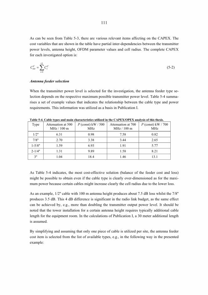
111

As can be seen from Table 5-3, there are various relevant items affecting on the CAPEX. The cost variables that are shown in the table have partial inter-dependencies between the transmitter power levels, antenna height, OFDM parameter values and cell radius. The complete CAPEX for each investigated option is:

�=

=12

1i

Ci

Ctot CC (5-2)

Antenna feeder selection

When the transmitter power level is selected for the investigation, the antenna feeder type se-lection depends on the respective maximum possible transmitter power level. Table 5-4 summa-rises a set of example values that indicates the relationship between the cable type and power requirements. This information was utilized as a basis in Publication I.

Table 5-4. Cable types and main characteristics utilized in the CAPEX/OPEX analysis of this thesis.

Type Attenuation at 500 MHz / 100 m

P (const) kW / 500 MHz

Attenuation at 700 MHz / 100 m

P (const) kW / 700 MHz

1/2'' 6.31 0.98 7.58 0.82 7/8'' 2.70 3.38 3.44 2.65

1-5/8'' 1.59 6.93 1.91 5.77 2-1/4'' 1.31 9.89 1.58 8.21

3'' 1.04 18.4 1.46 13.1

As Table 5-4 indicates, the most cost-effective solution (balance of the feeder cost and loss) might be possible to obtain even if the cable type is clearly over-dimensioned as for the maxi-mum power because certain cables might increase clearly the cell radius due to the lower loss.

As an example, 1/2'' cable with 100 m antenna height produces about 7.5 dB loss whilst the 7/8'' produces 3.5 dB. This 4 dB difference is significant in the radio link budget, as the same effect can be achieved by, e.g., more than doubling the transmitter output power level. It should be noted that the tower installation for a certain antenna height requires typically additional cable length for the equipment room. In the calculations of Publication I, a 30 meter additional length is assumed.

By simplifying and assuming that only one piece of cable is utilized per site, the antenna feeder cost item is selected from the list of available types, e.g., in the following way in the presented example:

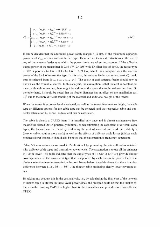
112

��

�

��

�

�

−=<−=<−=<

−=<−=<

=−

−

−−

εεε

εε

kWPPmckWPPmckWPPmc

kWPPmckWPPmc

C

TX

TX

TX

TX

TX

C

09.13,/21.8,/77.5,/

65.2,/82.0,/

''3max''3

''4/12max''4/12

''8/51max''8/51

''8/7max''8/7

''2/1max''2/1

3 (5-3)

It can be decided that the additional power safety margin ε is 10% of the maximum supported power level Pmax of each antenna feeder type. There are no technical restrictions in the use of any of the antenna feeder type whilst the power limits are taken into account. If the effective output power of the transmitter is 2.16 kW (2.4 kW with TX filter loss of 10%), the feeder type of 7/8'' supports 2.65 kW – 0.1·2.65 kW = 2.39 kW, which thus complies with the realistic power of the 2.4 kW transmitter type. In this case, the antenna feeder and related cost CC3 could thus be selected from {c7/8'', c1-5/8'', c2-1/4'', c3''}. The cost c of each antenna feeder should now be known via the available sources. In this analysis, the assumption is that the cost is constant per meter, although in practice, there might be additional discounts due to the volume purchase. On the other hand, it should be noted that the feeder diameter has an effect on the installation cost

CC4 due to the more difficult handling of the material and additional weight of the feeder.

When the transmitter power level is selected, as well as the transmitter antenna height, the cable type or different options for the cable type can be selected, and the respective cable and con-nector attenuation Lcc as well as total cost can be calculated.

The cable is clearly a CAPEX item. It is installed only once and is almost maintenance free, making the related OPEX practically minimal. When estimating the cost effect of different cable types, the balance can be found by evaluating the cost of material and work per cable type (heavier cable requires more work) as well as the effects of different cable losses (thicker cable produces lower losses). It should also be noted that the attenuation is frequency dependent.

Table 5-5 summarises a case used in Publication I by presenting the site cell radius obtained with different cable types and transmitter power levels. The assumption is to use all the antennas in 100 m tower. This table indicates that the cable types of {1-5/8'', 2-1/4'', 3''} provide similar coverage areas, so the lowest cost type that is supported by each transmitter power level is an obvious selection in order to optimize the cost. Nevertheless, the table shows that there is a clear difference between {1/2'', 7/8'', 1-5/8''}, the thinner cable producing clearly lower coverage ar-eas.

By taking into account this in the cost analysis, i.e., by calculating the final cost of the network if thicker cable is utilized in these lower power cases, the outcome could be that the thicker ca-ble, even the resulting CAPEX is higher than for the thin cables, can provide more cost-efficient OPEX.

113

Table 5-5. An example of the site cell radius obtained by varying the cable type and transmitter power levels. N/A is shown if the cable is not suitable for the respective power level.

Cell range (km) for cable type of: PTX / W

1/2" 7/8" 1-5/8" 2-1/4" 3"

100 3.7 5.6 6.4 6.6 6.7 200 4.6 6.9 8.0 8.3 8.4 500 6.2 9.2 10.7 11.0 11.1 750 7.0 10.5 12.1 12.5 12.7

1500 N/A 13.0 15.1 15.6 15.7 2800 N/A N/A 18.4 18.9 19.2 3400 N/A N/A 19.5 19.9 20.0 4700 N/A N/A 20.4 20.6 20.7 9000 N/A N/A N/A N/A 22.6

OPEX items

Table 5-6 summarizes the OPEX items that were utilized in the cost analysis of Publication I. As was the case in CAPEX item identification, also the OPEX items were selected according to the realistic deployment.

Table 5-6. The most relevant OPEX items and relations. Variable OPEX item Observations

OC1 Electricity The electricity consumption depends mainly on the transmitter type (power level) as well as the power consumption of the related other site elements like modulator, site cooling system, routers etc.

OC2 Maintenance The maintenance includes principally the transmitter maintenance that depends on the complexity of the transmitter. As an example, air cooled requires less site visits than oil cooled, which in turn also requires oil changes.

OC3 Transmission The transmission can be either terrestrial or via satellite. Both have cost effect, terrestrial triggering site specific costs whilst the costs of a single satellite usage can be divided between all the respective sites.

OC4 Tower / site rent If no own site or tower has been obtained, the rental costs of the equipment shelter and / or antenna system usage are added to the OPEX.

OC5 Other expenses Any other item triggering regular costs like average level of the general site maintenance.

The electrical power consumption Pc of the transmitters can be estimated in a general level as a function of the transmitter output power level, unless there is no more accurate estimate avail-able:

114

TXc PP ⋅= 6 (5-4)

The yearly cost of the transmitter with a power level of PTX is thus:

1000/3652461 ⋅⋅⋅⋅= hcPC eTXO , (5-5)

where ce is the cost of electricity per kWh. Equally, the other OPEX items should be estimated in absolute values in yearly basis, which results in the total OPEX per year:

�=

=5

1/

i

Oi

Oyeartot CC (5-6)

The yearly costs might vary over the time, but in this level analysis it is sufficient to estimate an average cost per year.

Combined CAPEX/OPEX of the whole network

When the CAPEX and OPEX are calculated for all the investigated options as a function of transmitter power levels (transmitter types), antenna heights and OFDM parameters (which re-sults in the balance between the capacity and coverage), the combined network cost can be cal-culated.

The single cell radius d, or the distance between the site and calculated cell edge with the given area location probability, indicates how many partially overlapping sites can be located within a certain area, which can be the whole planned network or part of that. By taking into account the overlapping share of the hexagonal model as presented in Figure 6-8 of the simulator Appendix, and in Figure 5 of Publication I, the number of the site cells Ncells is:

827.0827.0 2 ⋅=⋅=cell

tot

cell

totcells d

AAAN

π , (5-7)

where Atot is the whole investigated area (km2) and Acell is the single site cell coverage area (km2). This information is the key for the CAPEX/OPEX analysis in Publication I as it provides the possibility to compare the efficiency of the selected parameters in order to minimize the cost when filling the area with the full coverage area.

The total cost of the investigated part of the network is thus:

( )yO

yeartotCtotcellstot NCCNC ⋅+⋅= / , (5-8)

where Ny is the number of the operating years with {Ny∈ℜ⏐0<Ny<tmax}, where tmax is the maxi-mum operating years of the network. The aim is now calculate as many options as are logical to investigate, by following the planning process from the beginning. The first task is to fix the

115

maximum offered capacity, which results in a certain limited set of OFDM parameter values for the modulation scheme, CR and MPE-FEC. The analysis can also be limited by selecting realis-tic general values for the possible maximum antenna heights in the investigated area. Also the regulatory radiation values might be needed to be taken into account when limiting the antenna heights and maximum possible radiating power levels.

The most logical set of parameters can now be tested by calculating the maximum path loss L and respective cell radius d, which gives the cost estimate for each case. The results of Publication I show that there is an optimal point in the combined CAPEX and OPEX curves when varying the transmitter powers. In the presented case analysis of Publication I, the optimal transmitter power class is found in mid-range models. A further analysis shows that the optimal point varies during the time, higher power transmitters becoming more cost-efficient solution in the longer run.

This outcome of the optimal power level which is not necessarily the highest possible one is an interesting deviation to the typically presented assumption which indicates that the optimization via the reducing of sites by increasing as high masts and as high output powers as possible is assumed to lead directly to the reduction of costs as presented, e.g. in [Hoi06, p.4].

CAPEX and OPEX (4 years)

0,1

1

10

100W 200W 500W 750W 1500W 2800W 3400W 4700W 9000W

h(ant)=50m

h(ant)=75m

h(ant)=100m

h(ant)=150m

h(ant)=200m

h(ant)=250m

h(ant)=300m

Figure 5-11. The cost effect of the DVB-H network when the antenna height is varied. This case includes relatively high transmission costs as utilized in Publication I.

116

There are many inter-dependencies between the variables which require various iteration rounds if the optimal set of parameter values are investigated thoroughly. As an example, by keeping the variables the same as in the presented example of Publication I, but varying the antenna height in a sub-urban area, Figure 5-11 can be obtained. The presented values are normalized to 500W-transmitter case and for the antenna height hant of 100 meters. The analysis shows the combined CAPEX and OPEX after 4 years of operation.

Figure 5-11 indicates that the higher the antenna is located the lower the cost of the network is. This is logical outcome because the coverage areas grow as a function of the antenna height. It is interesting to note though, that in this specific case and in a range of about 75...150 meters of antenna height, the optimal transmitter power level is in mid-range models whereas in lowest and highest antenna locations the high-power solution is the optimal in each antenna height category.

For the high antenna cases this is understandable as the number of high-power transmitters is relatively low in order to achieve the same coverage area as with the lower power cases. The explanation for the low antenna height behaviour is that the number of the high-power sites in that specific situation is low enough to favour the high-power transmitters even if their relative cost of power consumption is clearly higher.

CAPEX and OPEX (4 yers), low transmission costs

0,1

1

10

100W 200W 500W 750W 1500W 2800W 3400W 4700W 9000W

h(ant)=50mh(ant)=75m


h(ant)=200m


, 4 years, CAPEX and OPEX (4 yers), low transmission costs

0,1

1

10

100W 200W 500W 750W 1500W 2800W 3400W 4700W 9000W



h(ant)=200m


, 4 years,

Figure 5-12. An example of the cost effect as a function of the antenna height when the transmission costs are assumed to be low.

117

In the above mentioned examples, the transmission cost has been assumed to be based on leased lines with relatively high cost (in order of 150,000 euros per year per site). The tower rental and site cost has been assumed to be in order of 20,000 euros per year. If the transmission cost can be reduced considerably, e.g. down to 15,000 euros per year per site, the result changes. This is due to the fact that the relative proportion of the electricity consumption gets much higher in the total OPEX. Figure 5-12 shows a related analysis, with all the other parameters being the same as in case of Figure 5-11.

The reference for the normalized y-values (costs) has been kept the same in Figure 5-12 as in Figure 5-11, i.e. the analysis is based on the 500 W transmitter case and for 100 meters of an-tenna height. As can be noted, the relative cost of the network is considerably lower with low transmission costs. In this case, the highest power case of 9,000 W results now in about 49 % of the OPEX out of the total operating expenses. This effect can be seen in Figure 5-12 as the opti-mal point per antenna height category is clearly indicating the mid-range power transmitters.

It is worth noting that the above mentioned analysis results in optimal transmitter power level and antenna height values, which in many cases indicates the mid-level range. As a comparison, [Mil06, p. 63] has identified the optimal point in mid antenna height in city area case, but the transmitter power seem to behave in linear way, i.e. the higher the power level is, the more eco-nomical the network cost is as the coverage areas of single site is large. The lack of clear opti-mal points indicates that the study might be missing of such detailed inputs that were used in Publication I. Furthermore, the operating costs were not taken into account in [Mil06, p. 63].

Cost optimisation in varying sites

The method shown in this thesis for the CAPEX/OPEX optimisation is based on the uniform parameter values over the whole investigated network. Nevertheless, the method can also be applied for the varying site configurations, e.g., in the environment presented in Publication VII. Furthermore, the analysis can be combined to the coverage area study, as well as to the SFN gain and SFN interference balancing study by varying the radio parameters and by calculating the respective costs either in uniform case or site-dependent parameter values.

Conclusions

As a conclusion of the cost optimisation, it is important to identify all the relevant cost items case-by-case and carry out the related analysis. If the DVB-H transmitter antennas can be lo-cated relatively high, it helps in the optimisation of the coverage areas. There are limits though, the increased power consumption being one of the critical items in the case of the highest power level transmitters. As Figure 5-11 and Figure 5-12 shows, the antenna height does have a considerable effect on CAPEX and OPEX and the optimal cost point can be found.

118

On the other hand, the optimal height might depend also on the other aspects like on the fine-tuning of the maximum size of the single frequency network, i.e. when sufficiently low EIRP levels are used, the theoretical SFN diameter is not necessarily a limit in practice and the single frequency can be used in large areas as shown in Chapter 5.1.1. An optimal solution would possibly include part of the antennas installed as high as possible to broadcast towers and others in telecom towers and rooftops due to the easier access.

Furthermore, there might be possibilities to adopt the transmit diversity for the DVB-H net-works. It would improve the reception and QoS in the site cell edges and the outage areas within the site cell. The technique provides thus a robust reception with improved QoS, and can reduce the network costs by lowering the transmit power and the number of infrastructure elements as has been noted in [Zha08, p. 575].

Reference [Hoi06] contains DVB-H specific techno-economic considerations. Nevertheless, the analysis it presents is not sufficiently detailed for the comparison of the results obtained in this thesis. Other highly relevant references for the comparison of the presented method and case results are [Gom06], [Gom07], [Joh07], and [Bri05]. They present analysis for the optimizing of the network deployment and operation costs, e.g., by comparing broadcast and mobile network towers and by combining DVB-H and other cellular systems infrastructure. Unfortunately, none of these considers a DVB-H network deployment scenario like presented in this thesis, making the final comparison of the results challenging.

As a conclusion of the cost optimisation part of this thesis, a sufficiently detailed method was developed to be taken into account in the typical DVB-H deployment. The other found refer-ences presented the related aspects either from purely economical point of view [Bal07] [Sat07], or taking into account only partially the relationship between cost and technical items [Bmc07] [Sat06] [Ski06]. Instead, this thesis presents a complete set of CAPEX and OPEX items which were investigated as a function of transmitter antenna height and power levels, taking into ac-count all the relevant deployment aspects of the equipment and planning environment in a more detailed way than was found in other related references.

119

6 Summary and conclusions

6.1 Main results of this thesis

As a basis for this thesis, a radio network planning and optimisation process chart was created for the nominal as well as for the detailed phase of the planning. The process modules were de-signed based of the publicly available information, but enhancing the processes. Based on these process charts, the methods of the most relevant parts of the processes were identified and in-vestigated. The outcome clarifies the DVB-H link budget usage. The results include the optimi-sation of the essential network parameter values taking into account the related network build-ing and operation costs, as well as the regulatory limitations of the radiation powers.

An enhanced methodology for the field measurements and analysis with hand-held DVB-H ter-minal was created. The outcome of this part was the introduction of the procedure for the meas-uring and post-processing of the field test data. Selected cases were carried out, and the respec-tive results can be used in order to fine-tune the radio link budget in similar locations the tests were performed. The closest similar analysis can be found in [Amp06a]. This thesis clarifies the way to present and interpret MPE-FEC gain, and gives a more detailed means for the estimation of the accuracy of the results.

A simulation method for the SFN investigations was developed and respective case studies were carried out by utilizing a set of practical parameter values. The method is based on the physical radio propagation analysis assuming that the upper layer functionality is ideal. The respective carrier-to-noise and carrier-to-interference ratios are assumed to be fixed for the used parame-ters. The method is thus valid for obtaining information about the limits of the network per-formance and is thus sufficiently accurate to select the optimal parameter values, e.g. as a func-tion of transmitter antenna height and power level. The initial version of the simulator is based on the hexagonal site cell layout, common antenna heights and power levels, but it was also shown that the tool can be utilized for more practical environments with individual site configu-rations.

One of the outcomes of the simulations was the confirmation that the large (over-sized) SFN network can be applied when the essential parameters are tuned correctly like the height of the antennas and radiating power levels of the transmitters. The used analysis method is slightly different than the found references because the comparative simulations are proposed to be done over the whole investigated area instead of individual sub-regions. The proposed method gives sufficiently accurate results for the comparison of different parameter settings, and the simula-tions require considerably less time than the sub-region method. Nevertheless, the results corre-

120

late with the outcome of the available reference material. Furthermore, the results show accept-able quality when the balance between the SFN gain and SFN interference levels are taken into account. The performance of the network can be further optimized by using directional anten-nas, down-tilting and case-by-case adjustment of the antenna directions by utilizing the topol-ogy of the surrounding areas. At the same time, the simulator shows the overall cumulative dis-tributions of C/N and C/(N+I) over the investigated area in numeric format as well as in visual format within the geographical area.

The simulator also shows the level of the SFN gain in a non-interfered DVB-H network. Al-though [Bmc09] recommends that the SFN gain should be set to zero in the radio link budget assumption, the results of this thesis indicate that the SFN gain can be taken into account in a sufficiently overlapping site cell layout. As one of the outcomes of the SFN gain related simula-tions, the definition of the SFN gain has been clarified. The method takes into account the com-bination of the gain and interference within the whole investigated network, not only non-inter-fered environment and in limited locations as the found other publications typically show.

6.2 Usability of the results

The results of this thesis can be used for the DVB-H network planning and optimisation which benefits primarily the network operators. The main focus of the thesis was to develop method-ologies that can be applied in arbitrary parameter value settings depending on the area and radio channel type. The numerical values are meant for examples, but as such they indicate that the adjustment of the DVB-H radio link budget accordingly is one of the most important tasks in the technical radio network planning. The results clearly show the importance of the selection of cost-effective assumptions in the network deployment, which is essential in the designing of the business models with efficient return of investment schemes.

By applying the presented methodologies for the measurements and simulations, it is possible to adjust the parameter values in an optimal way in each environment of the commercial networks. The presented methods for the field tests as well as for the SFN interference estimate can be proposed as complementary modules for the typical network planning process, giving added value especially in the beginning of the deployment due to their time savings. The proposed field test method eases and speeds considerably the data collection and analysis compared to the more in-depth studies, yet providing sufficiently information in order to, e.g. eliminate the less feasible parameter values already in the early stage of the planning. The simulation method, on the other hand, complements the usual area element based coverage planning. It provides the first-hand comparative results for the selection of the functional SFN interference levels in a considerably faster time than the traditional coverage planning programs do. This outcome can be utilized, again, for rejecting the least feasible parameter values, and the more accurate and

121

time consuming coverage investigation can the be made by applying the traditional area element approach for the most suitable values obtained via the proposed method.

6.3 Further study items

The transmitter diversity in DVB-H can increase the network performance with several decibels as has been concluded in [Zha06]. It would be interesting to take into account the balance of SFN gain and SFN interference level in over-dimensioned SFN networks that uses transmitter diversity. The SFN simulator presented in Publications III, and IV could thus be enhanced in order to obtain the optimal parameter settings, transmitter antenna height and transmitter power.

The quality criterion of DVB-H has been studied in [Him09]. Even this thesis uses the typical error criteria presented in [Dvb09], the frame error rate before and after MPE-FEC being the most important, there might be parallel criteria that reflect the service quality better as stated in [Him06]. Based on the experiences during the field measurement with the methodology pre-sented in Publication II, it seems that the BER before and after Viterbi are not reliable criteria especially in the edge of the coverage area as the algorithm for calculating the error rate in ter-minal or measurement equipment side is inaccurate due to the lack of information of correct and erroneous data. Furthermore, based on the observations of Publication II it seems justified to claim that frame error rate gives practical indication about the quality level that the end-user can observe. This is due to the fact that if the frame is erroneous, it is seen immediately in the termi-nal side as non-fluent streaming of audio and/or video.

The MPE-FEC receiver is implementation dependent and decides what the streamer should do when erroneous frame is detected. In some cases, according to [Him06], it might be more bene-ficial to simply accept the erroneous frame and stream it in any case as the end-user might be less disturbed about the small occurred error than losing the whole frame. The practical limit of acceptable level of passing these erroneous frames is an interesting further study item in order to optimize the quality of the service in the terminal side.

Other items for potential further study that are not much reported are listed below:

− The effect of hierarchical modulation on DVB-H. The hierarchical modulation has been designed for the DVB-T and might thus be considered as a relatively complicated item in DVB-H environment with varying radio conditions, but a further study could bring deeper understanding about any benefits hierarchical modulation could bring in certain network areas.

− Advanced measurement methodologies that include MER, i.e. vector error mapping to the quality level that the end-user experiences. The frequency response information could first be used in the measurements by identifying the number and characteristics of

122

different components. This information could further be used for the MER / vector error or other information in order to get the perceived error effect. The clarified method could explain the degraded MER performance of SFN gain analysis that is presented in [Bov09].

− A further techno-economic study by taking into account a realistic map (either realistic site distribution or hexagonal). The map could include a candidate site rings. The analy-sis could be carried out by switching on and off different sites according to the func-tional site combinations, and tune the complete set of parameters of each site separately. Different radio propagation models can be used individually for each site depending on the surrounding environment, cluster type, topography etc. By iterating, and taking into account the radiation limitations (regulatory limits), and cost optimisation, it would be possible to search for parameter combinations that comply with the quality criteria and minimize costs over the investigated time period. As a continuum, a complete techno-economical optimisation tool could be created that integrates an iterative CAPEX / OPEX analysis based on the technical parameter selection and SFN gain/interference simulator and a commercial coverage planning tool.

− More detailed level simulations in link level might be interesting to design by applying the same physical level ideas as presented in this thesis. The idea would be to create complete DVB-H frames with varying error correction schemes. The frames could be created by utilizing real audio / video contents that is encoded, or samples of the real frames. When the frames are distributed over the radio interface, a bit error rate can be applied depending on the radio conditions, i.e. fading profile, signal level and the pres-ence of interferences. The error rate could be applied on bit-by-bit basis, and study the error correction capability in the receiving end. Furthermore, more realistic fading schemes could be applied in the simulator by taking into account the frequency selec-tivity in the Rayleigh channel, and by modelling real measured fading data from the in-vestigated area type.

123

References

[Apa06a] Maite Aparicio (editor). Wing TV. Services to Wireless, Integrated, Nomadic, GPRS, UMTS & TV handheld terminals. D6: Common field trials report. Novem-ber 2006. 86 p.

[Apa06b] Maite Aparicio (editor). Wing TV. Services to Wireless, Integrated, Nomadic, GPRS, UMTS & TV handheld terminals. Wing TV Country field trial report. No-vember 2006. 258 p.

[Apt06] APT Recommendation on Guidelines for the Frequency Coordination for the Terrestrial Services at the Border Areas Between Administrations. No. APT / AWF / 2. Edition: Asia-Pacific Telecommunity. The APT Wireless Forum February 2006. Approved By The 30th Session of the APT Management Committee 18 – 21 Sep-tember 2006 Maldives.

[Aur09] Interview of Tommi Auranen, Nokia, Salo, Finland. 15.12.2009.

[Avo06] Peter MacAvock. The DVB-H Experience. 3GSM ’06 Barcelona. 15th February 2006. 12 p.

[Bac04] Wenche Backman. Signal Level Interpolation for Coverage Area Prediction. 0-7803-8521-7/04. IEEE 2004. Pp. 67-71.

[Bal07] Gian Paolo Balboni. How Advertising Revenues Can Increase Profitability of DVB-H Services. Presentation, Deploying and Managing DVB-H, Gruppo Telecom Italia. London, September 27, 2007. 33 p.

[Bar06] David Gómez-Barquero, Aurelian Bria, José F. Monserrat, Narcis Cardona. Minimal cost planning of DVB-H networks on existing wireless infrastructure. IEEE 17th International Symposium on Personal, Indoor and Mobile Radio Communications 2006. Pages 1-5.

[Bar07] David Gómez-Barquero, Narcís Cordona, Aurelian Bria, Jens Zander. Affordable mobile TV services in hybrid cellular and DVB-H systems.

[Bee02] J. J. van de Beek, P. Ödling, S. K. Wilson, P. O. Börjesson. Orthogonal Frequency-Division Multiplexing (OFDM). International Union of Radio Science (URSI). 2002.

[Bee07] Karina Beeke. Spectrum Planning — Analysis of methods for the summation of Log-normal distributions. EBU technical review– October 2007. 9 p.

124

[Bee98] Jan-Jaap van de Beek. Synchronization and Channel Estimation in OFDM Systems. PhD thesis, Lulea University of Technology, Division of Signal Processing, Lulea, Sweden. 1998. 158 p.

[Bmc07] Claus Sattler. Mobile Broadcast Business Models. A State of the Art Study. BMCOFORUM, November 2006. 36 p.

[Bmc07b] Spectrum Position for Mobile TV. BMCOFORUM, March 2007. 4 p.

[Bmc07c] Mobile Broadcast Bearer Technologies – A Comparison. BMCOFORUM, January 2007. 58 p.

[Bmc09] Link Budgets. Update 02/2009. BMCOFORUM, February 2009. 178 p.

[Bou06] Thibault Bouttevin (editor). D8 - Wing-TV Measurement Guidelines & Criteria. Wing TV. Services to Wireless, Integrated, Nomadic, GPRS, UMTS & TV hand-held terminals. June 2006. 45 p.

[Bou08] Imed Bouazizi, Miska Hannuksela, Lukasz Kondrad, Moncef Gabbouj. Efficient FEC Protection of Scalable Media Streams in DVB-H. BTS08, Alexandria, USA. 6 p.

[Bov09] Jose Bóveda, Gorka Marcos, Jesús Maria Pérez, Sara Ponce, Ane Aranaz. MER degradation in a Broadcast Mobile Network. IEEE International Symposium on Broadband Multimedia Systems and Broadcasting (Broadband Multimedia 2009). Bilbao, Spain, 13-15 May, 2009. 5 p.

[Bri05] Aurelian Bria, David Gómez-Barquero. Scalability of DVB-H deployment on existing wireless infrastructure. IEEE 16th International Symposium on Personal, Indoor and Mobile Radio Communications 2005. Pages 716-720.

[Bro02] P. G. Brown, K. Tsioumparakis, M. Jordan, A. Chong. UK Planning Model for Digital Terrestrial Television Coverage. Esearch & Development. White Paper WHP 048. September 2002. 12 p.

[Bro08] Petter Brodal, Henning Gundersen, Gunn Kristin Klungsøyr. DVB-H technology overview. R&I N 24/2008. R&I Research Note. ISSN 0809-1021. 11.4.2008. 43 p.

[Cha06] Joo Chan Kim, Jin Young Kim. Single Frequency Network Design of DVB-H (Digital Video Broadcasting – Handheld) System. ICACT2006. February 20-22, 2006. Pp. 1595-1598.

[Che85] David R. Cheriton, Stephen E. Dewing. Host groups: A Multicast Extension for Datagram Internetworks. Report No. STAN-CS-85-1058 (also numbered CSL-85-280). Department of Computer Science, Stanford University. July 1985. 9 p.

125

[Chu00] Arto Chubukjian, Hughes Nappert, Kirit Mehta, Andrk Legris. An example of effi-cient spectrum management: Army tactical radio operations in broadcasting bands. Industry Canada, Ottawa, Ontario, Canada. 0-7803-6521-6. IEEE, 2000. Pp 15-18.

[Cos99] Digital Mobile Radio Towards Future Generation Systems. COST 231 Final Re-port. COST/EC, Brussels, Belgium, 1999. 474 p.

[Dig05] Television on a handheld receiver – broadcasting with DVB-H. Digital Terrestrial Television Action Group. Version 1.2, Grand-Saconnex, Geneva, Switzerland, 2005. 24 p.

[Dvb04] Digital Video Broadcasting (DVB); Transmission System for Handheld Terminals (DVB-H). ETSI EN 302 304, V1.1.1 (2004-11). 14 p.

[Dvb06] DVB-H Implementation Guidelines. Draft TR 102 377 V1.2.2 (2006-03). European Broadcasting Union, March 2006. 108 p.

[Dvb06b] Digital Video Broadcasting (DVB); IP Datacast over DVB-H: Architecture. ETSI TR 102 469 V1.1.1 (2006-05). 28 p.

[Dvb06c] Digital Video Broadcasting (DVB); IP Datacast over DVB-H: Use Cases and Ser-vices. ETSI TR 102 473 V1.1.1 (2006-04). 29 p.

[Dvb07] IP Datacast over DVB-H: Implementation Guidelines for Mobility. DVB Document A117 (BlueBook), July 2007. 26 p.

[Dvb07b] Digital Video Broadcasting (DVB); IP Datacast over DVB-H: Set of Specifications for Phase 1. ETSI TS 102 468 V1.1.1 (2007-11). 8 p.

[Dvb08] Broadcasting to Handhelds. DVB Fact Sheet, August 2008. Produced by the DVB Project Office. 2 p.

[Dvb09] Digital Video Broadcasting (DVB); DVB-H Implementation Guidelines. ETSI TR 102 377 V1.3.1 (2009-03). 114 p.

[Ebu05] BPN – 066, issue 1.0, guide of SFN Frequency Planning and Network Implementa-tion with regard to T-DAB and DVB-T, EBU – technical department 2005, 124 p.

[Ebu09] General issues to be considered when planning SFNs. EBU Technical Media Tech-nology & Innovation. 13 March 2009. 5 p.

[Ecc04] ECC Report 49. Technical Criteria of Digital Video Broadcasting Terrestrial (DVB-T) and Terrestrial – Digital Audio Broadcasting (T-DAB) Allotment Planning. Electronic Communications Committee (ECC) within the European Conference of Postal and Telecommunications Administrations (CEPT) Copenhagen, April 2004. 36 p.

126

[Fan06a] Myron D. Fanton. Analysis and Measurement of RF System Reflections and DTV Transmission. Electronics Research, Inc. ERI Technical Series, Vol. 6, April 2006. 7 p.

[Fan06b] Myron D. Fanton. Analysis of Antenna Beam-tilt and Broadcast Coverage. Elec-tronics Research, Inc. ERI Technical Series, Vol. 6, April 2006. 3 p.

[Far01] Gerard Faria. Mobile DVB-T using antenna diversity receivers. IBC 2001. Amster-dam, September 2001. 11 p.

[Far04] Gerard Faria. DVB-H to deliver Digital TV to Hand-Held Terminals. IBC 2004. September 2004, Amsterdam. 12 p.

[Far05] Gerard Faria. DVB-H: Digital TV in the hands. IBC’05, Amsterdam, September 2005. 12 p.

[Far05b] Gerard Faria. The handheld world outside – DVB-H. Presentation material, DVB World 2005, 4th March 2005, Dublin. 27 p.

[Far05c] Gerard Faria. Validation Task Force Field Trials. Embedded Systems Conference – 3G Cellular System Design Seminar. March 2005. 17 p.

[Far06] Gerard Faria, Jukka A. Henriksson, Erik Stare, Pekka Talmola. DVB-H: Digital Broadcast Services to Handheld Devices. Proceedings of the IEEE, Vol. 94, No. 1, January 2006. Pp 194-209.

[Far07] Gerard Faria. From Digital TV to Mobile TV. CSTB’07 – Media on the Move – DVB tutorial. 5th February 2007. 48 p.

[Fcc07] Federal Communications Commission. Report and order and further notice of pro-posed rulemaking (FCC 07-72). Adopted: April 25, 2007. Released: April 27, 2007. 191 p.

[Fcc98] Federal Communications Commission, Office of Engineering & Technology. Washington, D.C. 20554. Information on Human Exposure to Radiofrequency Fields from Cellular and PCS Radio Transmitters. January 1998.

[Fis08] R. Fuschini, H. El-Sallabi, V. Degli-Esposti, L. Vuokko, D. Guiducci, P. Vaini-kainen. Analysis of multipath propagation in urban environment through multidi-mensional measurements and advanced ray tracing simulation. IEEE Transactions on Antennas and Propagation, Vol. 56, no. 3, 2008. Pp. 848-857.

[Fis08] Walter Fischer. Digital Video and Audio Broadcasting Technology. A Parctical Engineering Guide. ISBN 978-3-540-76357-4. 2008, Spriner-Verlag Berlin Heidel-berg. 580 p.

[Gar07] G. Gardikis, H. Kokkinis, G. Kormentzas. Evaluation of the DVB-H Data Link Layer. European Wireless 2007. 1–4 April 2007, Paris, France. 6 p.

127

[Goe02] Roland Götz. Supporting Network Planning Tools II. Presentation, LS telcom AG, 2002. 38 p.

[Gom07] David Gómez-Baquero, Aurelian Bria. Forward Error Correction for File Delivery in DVB-H. Polytechnic University of Valencia, Spain, and Royal Institute of Tech-nology, Sweden. Vehicular Technology Conference VTC 2007, Spring. Dublin, 22-25 April 2007. 5 p.

[Gom09] David Gómez-Baquero. Cost efficient provisioning of mass mobile multimedia services in hybrid cellular and broadcasting systems. Doctoral dissertation in telecommunications. Universidad Politecnica de Valencia, Departamento de Comunicaciones. Valencia, Spain, 2009. 160 p.

[Goz08] David Gozálvez, David Gómez-Barquero, Narcis Cardona. Performance Evaluation of the MPE-iFEC Sliding RS Encoding for DVB-H Streaming Services.PIMRC’08. 5 p.

[Gre06] Emmanuel Grenier. DVB-H radio planning aspects in ICS telecom. White paper, ATDI. July 2006. 39 p.

[Had07] Kamel Haddad. DVB-H in Denmark. Technical and Economic aspects. Master’s Thesis. Technical University of Denmark (DTU), Center for Information & Com-munication Technologies (CICT). September 10, 2007. 98 p.

[Hat80] Masaharu Hata. Empirical Formula for Propagation Loss in Land Mobile Radio Services. IEEE Transactions on Vehicular Technology, Vol. VT-29, No. 3, August 1980. 9 p.

[Hen05] Jukka Henriksson. DVB-H standard, principles and services. HUT seminar T-111.590, presentation. Helsinki, 24.2.2005. 53 p.

[Him06] Heidi Himmanen, Ali Hazmi, Jarkko Paavola. Comparison of DVB-H link layer FEC decoding strategies in a mobile fading channel. The 17th Annual IEEE Inter-national Symposium on Personal, Indoor and Mobile Radio Communications (PIMRC'06). 1-4244-0330-8/06. IEEE 2006. 5 p.

[Him09] Heidi Himmanen. On Transmission System Design for Wireless Broadcasting. Aca-demic dissertation. University of Turku Department of Information Technology Turku, Finland, 2009. 165 p.

[Hoi06] Anssi Hoikkanen. Economics of wireless broadcasting over DVB-H networks. Wireless Telecommunications Symposium 2006. Pages 1-5.

[Hum09] The limits to terrestrial television’s case for further spectrum. Human Capital. February 2009. 31 p.

128

[Ili08] Teodor Iliev, Dimitar Radev, Izabella Lokshina, Georgi Hristov. Analysis and Evaluation of Reed–Solomon Codes in Digital Video Broadcasting Systems. Wire-less Telecommunications Symposium WTS 2008. 24-26 April 2008. Pp. 92-96.

[Itu07] Recommendation ITU-R P.1546-3. Method for point-to-area predictions for terres-trial services in the frequency range 30 MHz to 3000 MHz. 2007. 57 p.

[Jeo01] Minseok Jeong, Bomson Lee. Comparison between Path-Loss Prediction Models for Wireless Telecommunication System Design. 0-7803-7070-8/01. IEEE 2001. Pp. 186-189.

[Joh07] Klas Johansson, Jens Zander, Anders Furuskär. Cost efficient deployment of hetero-generous wireless access networks. IEEE 65th Vehicular Technology Conference 2007. Pages 3200-3204.

[Jok05] Heidi Joki, Jarkko Paavola, Valery Ipatov. Analysis of Reed-Solomon Coding Combined with Cyclic Redundancy Check in DVB-H link layer. ISWCS05. 0-7803-9206-X/05. IEEE 2005. Pp 313-317.

[Jok06] Tero Jokela, Jarkko Paavola, Heidi Himmanen,Valery Ipatov. Performance of Different Reed-Solomon Erasure Decoding Strategies at the DVB-H Link Layer. The 17th Annual IEEE International Symposium on Personal, Indoor and Mobile Radio Communications (PIMRC’06). 1-4244-0330-8/06. IEEE 2006. 5 p.

[Jos07] Wout Joseph, Emmeric Tanghe, Daan Pareit, Luc Martens. Building penetration measurements for indoor coverage prediction of DVB-H systems. 1-4244-0878-4/07. IEEE 2007. Pp. 3005-3008.

[Kru05] Stefan Krueger. DVB-H Pilot Berlin. Presentation. T-Systems International GmbH Media&Broadcast, Broadcast Network & Services. September 2005. 23 p.

[Law01] Eric Phillip Lawrey Be. Adaptive Techniques for Multiuser OFDM. Doctoral thesis. School of Engineering, James Cook University, 2001. 327 p.

[Lee86] William C.Y. Lee. Elements of Cellular Mobile Radio System. IEEE Transactions on Vehicular Technology, Vol. VT-35, No. 2, May 1986. pp. 48-56.

[Lig00] Agnes Ligeti. Outage Probability in the Presence of Correlated Lognormal Useful and Interfering Components. IEEE Communications Letter, Vol. 4, No. 1, January 2000. Pp. 15-17.

[Lig99a] Agnes Ligeti, Jens Zander. Minimal Cost Coverage Planning for Single Frequency Networks. IEEE Transactions on Broadcasting, Vol. 45, No. 1, March 1999. Pp. 78-87.

[Lig99b] Agnes Ligeti. Coverage Probability Estimation in Single Frequency Networks in Presence of Correlated Useful and Interfering Components. VTC 1999. Pp. 2408-2412.

129

[Lig99c] Agnes Ligeti. Single Frequency Network Planning. PhD thesis. Royal Institute of Technology. 1999. 175 p.

[Lun06] Janne Lundberg. A Wireless Multicast Delivery Architecture for Mobile Terminals. Dissertation for the degree of Doctor of Science in Technology. Helsinki University of Technology (Espoo, Finland) on the 15th of May, 2006. 138 p.

[Mäk05] Juri Mäki. Finnish Mobile TV Pilot Results. August 30th, 2005. Research Interna-tional Finland. 13 p.

[Mar05] Peter Marshall. Digital Television Project. Advanced Receiver Techniques with emphasis on Portable TV Reception. Issue 1.1. DTG Management Services Ltd, March 2005. 65 p.

[Mil06] Davide Milanesio (editor). Wing TV. Services to Wireless, Integrated, Nomadic, GPRS, UMTS & TV handheld terminals. D11 – Wing TV Network Issues. May 2006. 140 p.

[Min99] Limits of Human Exposure to Radiofrequency Electromagnetic Fields in the Fre-quency Range from 3 kHz to 399 GHz. Safety Code 6. Environmental Health Di-rectorate, Health Protection Branch. Publication 99-EHD-237. Minister of Public Works and Government Services, Canada 1999. ISBN 0-662-28032-6. 40 p.

[Nok05] Technical data sheet of Nokia N-92. Nokia, 2005. 1 p.

[Paa06] Paavola, J. (Editor); Kornfeld, M.; Rinne, J.; Björkqvist, J. Simulation Report. Deliverable D15, August 2006, EU CELTIC Project Wing TV. 67 p. http://projects.celtic-initiative.org/WING-TV.

[Pal08] Gema Roig Pallardó. On DVB-H Radio Frequency Planning: Adjustment of a Propagation Model Through Measurement Campaign Results. Master’s Thesis, University of Gävle, March 2008. 78 p.

[Pek05] Stuart Pekowsky, Khaled Maalej. DVB-H architecture for mobile communications systems. RF Design, April 2005. Pp 36-42.

[Pen09] Jyrki T.J. Penttinen, Petri Jolma, Erkki Aaltonen, Jani Väre. The DVB-H Hand-book. The Functioning and Planning of Digital Mobile TV. ISBN 978-0-470-74829-9. Wiley 2009. 236 p.

[Pen99] Jyrki Penttinen. The effects of the new data services on the GSM radio network planning. Licentiate thesis. Helsinki university of Technology. 1999.

[Pen99b] Jyrki Penttinen. Effects of GPRS on GSM Radio Network. International Conference on Telecommunications (ICT). Acapulco, Mexico, 2000. 5 p.

[Pir99] Riku Pirhonen, Tapio Rautava, Jyrki Penttinen. TDMA Convergence for Packet Data Services. IEEE Personal Communications. June 1999. pp. 68-73.

130

[Pit09] Renaud-Alexandre Pitaval. Relay Deployment in Single Frequency Network. Mas-ter's thesis. Helsinki University of Technology, Faculty of Electronics, Communi-cations and Automation, Department of Signal Processing and Acoustics, 2009. 101 p.

[Ple08] David Plets, Leen Verloock, Wout Joseph, Luc Martens, Etienne Deventer, Hugo Gauderis. New Method to Determine the SFN Gain of a DVB-H Network with Multiple Transmitters. 58th Annual IEEE Broadcast Symposium. 15-18 October 2008. Alexandria, VA, USA. 4 p.

[Ple09] David Plets, Leen Verloock, Wout Joseph, Luc Martens. Influence of DVB-H Net-work Deployment on Total RF Exposure. Proceedings, 20th Int. Zurich Symposium on EMC, Zurich 2009. Pp 329-332.

[Ple09b] David Plets, Leen Verloock, Wout Joseph, Luc Martens, Etienne Deventer, Hugo Gauderis. Weighing the Benefits and Drawbacks of an SFN by Comparing Gain and Interference caused by SFN Operation. IEEE International Symposium on Broadband Multimedia Systems and Broadcasting (Broadband Multimedia 2009). Bilbao, Spain, 13-15 May, 2009. 5 p.

[Pos05] Renzo Posega. Advanced OFDM Systems for Terrestrial Multimedia Links. Doc-toral thesis No. 3220/2005. École polytechnique fédérale de Lausanne. 194 p.

[Reg02] Decree on the limitation of exposure of the public to non-ionizing radiation 294/2002, based on the law on radiation protection 592/1991, 43.

[Rei05] Ulrich Reimers. DVB – The Family of International Standards for Digital Video Broadcasting. Second Edition. ISBN 3-540-43545-X. Springler-Verlag Berlin Hei-derberg 2005. 408 p.

[Rei06] Ulrich Reimers. DVB-H and IP Datacast: Technologies for Broadcasting to Hand-held Devices. Beijing, 22 November 2006. 26 p.

[San05] Finnish Mobile TV: Analysis on log file data. April – June 2005. Press event 30.8.2005. 16 p.

[Sat06] Claus Sattler. Mobile Broadcast Business Models: A State of the Art Study. BMCOFORUM, November 2006. 36 p.

[Sat07] Claus Sattler. Mobile Broadcasting: Trends and Challenges. LS Summit. 20. June 2007, Lichtenau. BMCOFORUM. 23 p.

[Sci07] Grzegorz Scibior. DVB-H Network Engineering – Link Budget & Human Exposure to EM fields prelUS 1.0. March 2007. Siemens Networks.

[Sil06] Airi Silvennoinen. DVB-H Network Optimization under Finnish Conditions (DVB-H –lähetysverkon optimointi Suomen olosuhteissa). Written in Finnish. Helsinki

131

University of Technology, Department of Electrical and Communications Engi-neering. Master’s Thesis. Espoo, Finland, 15.5.2006. 111 p.

[Ski06] Daniel Skiöld. An economic analysis of DAB & DVB-H. EBU Technical Review – January 2006. 10 p.

[Tal10] Interviews of Pekka H. K. Talmola, Finland, March 2010.

[Tun05] Celal Alp Tunc, Ayhan Altintas, Vakur B. Ertürk. Examination of Existent Propagation Models Over Large Inhomogeneous Terrain Profiles Using Fast Inte-gral Equation Solution. IEEE Transactions on Antennas and Propagation, Vol. 53, No. 9, September 2005. Pp. 3080-3083.

[Ung06] Peter Unger, Thomas Kürner. Radio Network Planning of DVB-H/UMTS Hybrid Mobile Communication Networks. Institut für Nachrichtentechnik (IfN), Tech-nische Universität Braunschweig, Germany. European Transaction on Telecommu-nication, special issue ETT 17-2, March 2006. pp.193-201.

[Ung08] Peter Unger, Thomas Kuerner. Optimizing the Local Service Areas in Single Fre-quency Networks. COST 2100 TD(08)467. Wroclaw, Poland, 2008/Febr/6-8. 7 p.

[Voj05] Ondrej Vojtko, Florian Makan. Radio Signal in WLAN Networks. Journal of Electrical Engineering, Vol. 56, No. 11-12, 2005. Pp. 331-332.

[Wan03] Xianbin Wang, Yiyan Wu, Jean-Yves Chouinard, Sili Lu, and Bernard Caron. A Channel Characterization Technique Using Frequency Domain Pilot Time Domain Correlation Method for DVB-T Systems. IEEE Transactions on Consumer Elec-tronics, Vol. 49, N0. 4, November 2003. Pp. 949-957.

[Zha06] Yue Zhang, John Cosmas, Maurice Bard, Yong-Hua Song. Diversity Gain for DVB-H by Using Transmitter/Receiver Cyclic Delay Diversity. IEEE Transactions on Broadcasting, Vol. 52, No. 4, December 2006. Pp 464-474.

[Zha08] Yue Zhang, C. Zhang, J. Cosmas, K. K. Loo, T. Owens, R. D. Di Bari, Y. Lostanlen, M. Bard. Analysis of DVB-H Network Coverage With the Application of Transmit Diversity. IEEE Transactions on Broadcasting, Vol. 54, No. 3. Septem-ber 2008. Pp. 568-576.

[Zir00] Single Frequency Network Concepts for cellular OFDM Radio Systems. Wolfgang Zirwas. Siemens AG, München. OFDM workshop, Hamburg, Germany, Sept. 2000. 4 p.

[Zyr98] Jim Zyren, Al Petrick. Tutorial on Basic Link Budget Analysis. Application note AN9804.1, Intersil, June 1998. 8 p.

[Öst06] Erik Östlin, Hajime Suzuki, Hans-Jürgen Zepernick. Evaluation of the Propagation Model Recommendation ITU-R P-1546 for Mobile Services in Rural Australia. 63rd IEEE Vehicular Technology Conference, Melbourne, Australia, May 2006.

132

Internet sources

Reference Link Contents, date of link validity revision

[web01] http://www.dvb-h.org Official web site of DVB-H project of-fice. 7.1.2011

[web02] http://www.dvb-h.org/services.htm Complete list of DVB-H networks that are launched or in trial stage. 7.1.2011

[web03] http://en.wikipedia.org/wiki/ Margin_of_error

Wikipedia pages for "Margin of error". 7.1.2011

[web04] http://www.bmcoforum.org Broadcast Mobile Convergence Forum. 7.1.2011

[web05] http://www.fcc.gov/oet/rfsafety USA regulations about the radiation safety limits. 7.1.2011

[web06] http://www.itu.int International Telecommunication Union. 7.1.2011

[web07] http://www.celtic-initiative.org/About_us/about.asp

Eureka cluster programme. 7.1.2011

[web08] http://ieeexplore.ieee.org/Xplore/ guesthome.jsp

IEEE Xplorer digital library. 7.1.2011

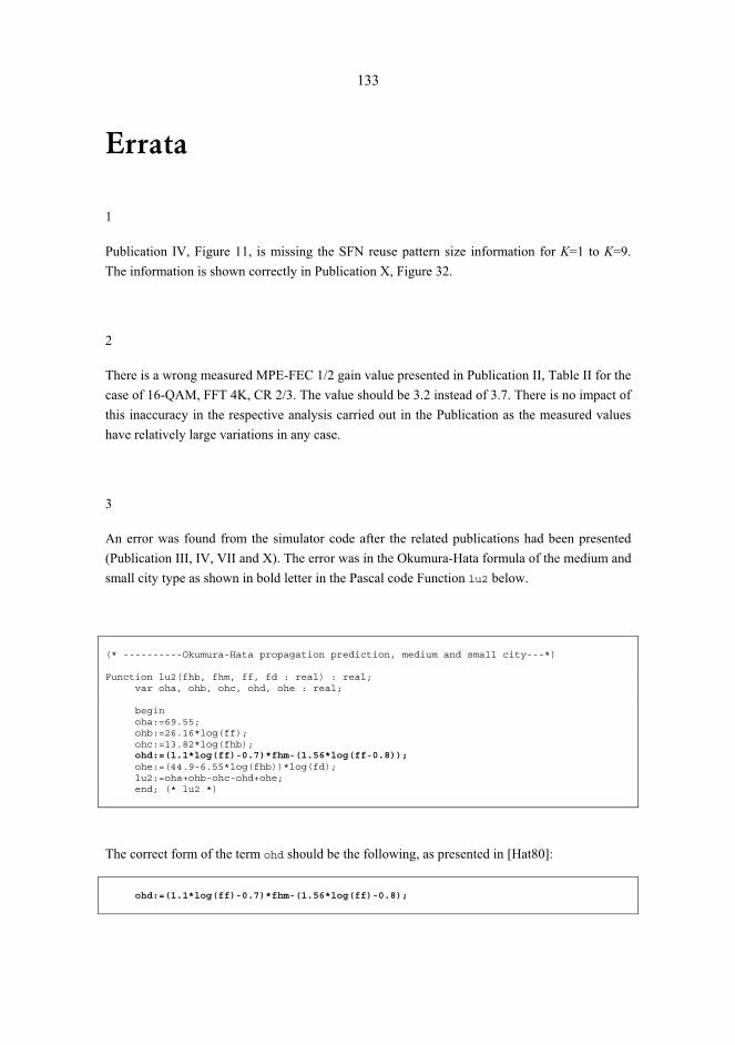
133

Errata

1

Publication IV, Figure 11, is missing the SFN reuse pattern size information for K=1 to K=9. The information is shown correctly in Publication X, Figure 32.

2

There is a wrong measured MPE-FEC 1/2 gain value presented in Publication II, Table II for the case of 16-QAM, FFT 4K, CR 2/3. The value should be 3.2 instead of 3.7. There is no impact of this inaccuracy in the respective analysis carried out in the Publication as the measured values have relatively large variations in any case.

3

An error was found from the simulator code after the related publications had been presented (Publication III, IV, VII and X). The error was in the Okumura-Hata formula of the medium and small city type as shown in bold letter in the Pascal code Function lu2 below.

(* ----------Okumura-Hata propagation prediction, medium and small city---*) Function lu2(fhb, fhm, ff, fd : real) : real; var oha, ohb, ohc, ohd, ohe : real; begin oha:=69.55; ohb:=26.16*log(ff); ohc:=13.82*log(fhb); ohd:=(1.1*log(ff)-0.7)*fhm-(1.56*log(ff-0.8)); ohe:=(44.9-6.55*log(fhb))*log(fd); lu2:=oha+ohb-ohc-ohd+ohe; end; (* lu2 *)

The correct form of the term ohd should be the following, as presented in [Hat80]:

ohd:=(1.1*log(ff)-0.7)*fhm-(1.56*log(ff)-0.8);

134

An analysis shows that the direct effect of the faulty formula is 0.799 dB for the L, when 700 MHz frequency is used in small and medium city area.

A snapshot investigation was made in order to evaluate the effect of the wrong formula. Five consecutive simulations were carried out with the erroneous formula, and other five simulations with the corrected version. The parameter values were selected in such a way that they are close to the previous simulation assumptions. An area of 100 km × 100 km was created with base sta-tion antenna height of 100 m, MS height of 1.5 m, MS antenna gain of �7 dBi, frequency of 700 MHz, standard deviation of 5.5 dB and TX power of +70 dBm. Rayleigh fading was not se-lected but large-scale fading was on. The area location probability was 90% in a small and me-dium city type with bandwidth of 8 MHz, modulation of QPSK, code rate of 1/2, MPE-FEC rate of 2/3, guard interval of 1/4 and FFT mode of 8K. The cumulative C/I distribution was investi-gated in such a way that the five simulation results were averaged per C/I (dB) value for the cor-rect version and for the erroneous version. By observing the mapping between the probability level and C/I, the following correction Tables can be formed to present the most important val-ues.

Table E-1. The C/I as a function of the probability scale. Probability C/I, correct C/I, faulty C/I, difference, correct

as reference

5% 9.5 dB 9.9 dB +0.4 dB 10% 13.5 dB 14.7 dB +1.2 dB 50% 22.7 dB 23.3 dB +0.6 dB

Table E-2. The C/I as a function of the probability scale. C/I Probability, correct Probability, faulty Probability,

difference, correct as reference

8.5 4.3 % 4.1 % –0.2 % units 14.5 12.0 % 9.7 % –2.3 % units 18.5 25.5 % 21.6 % –3.9 % units

As can be noted, the investigated probability per C/I value, i.e. the minimum limit for certain C/I, has been slightly optimistic. This does not have major impact on the previously presented results, though. Publication IV takes into account the balance of the SFN gain due to the over-lapping areas as well as for the loss of the gain due to the SFN interference. Slight difference in the mapping of absolute C/I values to the probability figures affects in both ways, so the relative balance of the gain and interference can be assumed to be practically unchanged. The impact of the error is not significant on the results of the Publication III either.

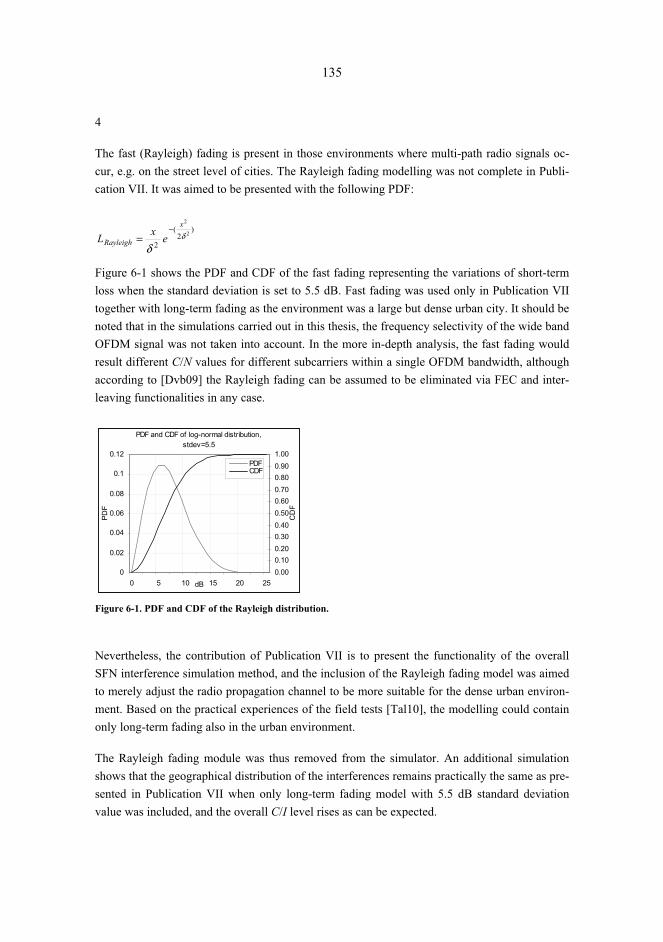
135

4

The fast (Rayleigh) fading is present in those environments where multi-path radio signals oc-cur, e.g. on the street level of cities. The Rayleigh fading modelling was not complete in Publi-cation VII. It was aimed to be presented with the following PDF:

)2

(

22

2

δ

δ

x

Rayleigh exL−

=

Figure 6-1 shows the PDF and CDF of the fast fading representing the variations of short-term loss when the standard deviation is set to 5.5 dB. Fast fading was used only in Publication VII together with long-term fading as the environment was a large but dense urban city. It should be noted that in the simulations carried out in this thesis, the frequency selectivity of the wide band OFDM signal was not taken into account. In the more in-depth analysis, the fast fading would result different C/N values for different subcarriers within a single OFDM bandwidth, although according to [Dvb09] the Rayleigh fading can be assumed to be eliminated via FEC and inter-leaving functionalities in any case.

PDF and CDF of log-normal distribution, stdev=5.5

0

0.02

0.04

0.06

0.08

0.1

0.12

0 5 10 15 20 25dB

PDF

0.000.100.200.300.400.500.600.700.800.901.00

CD

F

PDFCDF

Figure 6-1. PDF and CDF of the Rayleigh distribution.

Nevertheless, the contribution of Publication VII is to present the functionality of the overall SFN interference simulation method, and the inclusion of the Rayleigh fading model was aimed to merely adjust the radio propagation channel to be more suitable for the dense urban environ-ment. Based on the practical experiences of the field tests [Tal10], the modelling could contain only long-term fading also in the urban environment.

The Rayleigh fading module was thus removed from the simulator. An additional simulation shows that the geographical distribution of the interferences remains practically the same as pre-sented in Publication VII when only long-term fading model with 5.5 dB standard deviation value was included, and the overall C/I level rises as can be expected.

136

5

An error was found in the power sum formula of the simulator. The original version suggested that the multi-propagated components of the DVB-H radio signal was possible to estimate in SFN by summing the components in squared form, i.e., by presenting the useful received signal as shown in Publication III, Formula (1). Equally, in order to estimate the C/(N+I) level, the original simulator was based on the assumption that the total received interfering power would be calculated in a squared form as shown in Publication III, Formula (2).

Nevertheless, the squared form is utilized in the summing of individual amplitudes of the signal, not for the power levels. The useful carrier signals between the multi-propagated components, as well as the interfering signals between each individual interferer, can be assumed to be non-coherent. A direct power summing should be applied for the received power calculation as indi-cated in [Ebu05]. This means that the useful total received power (W) is:

�=

=n

iC

totC

iPP

1

(6-1)

Equally, the total received power (W) of the interfering components is:

�=

=n

iI

totI

iPP

1

(6-2)

When comparing the squared and direct form, it can be seen that the error for the estimate of the received power level is highest when two or more signal components are received at the same level. As an example, a practical worst case can be assumed to occur in the overlapping area of three sites where the signal level is the same. Assuming the received power level is �90 dBm for a parameter set of {QPSK, CR=1/2, MPE-FEC=1/2, GI=1/4} in such a location, the received total power of these three signals would result in the total power values by applying the squared and direct power summing as presented in Table 6-1. The received power level in dBm is con-verted to absolute powers (W) for the summing, and the result is converted back to dBm form by applying the formula PRX[dBm]=10log10(PRX[W]/1mW).

Table 6-1. Comparison of the squared and direct power summing. )(

1dBmPC

Signal 1

)(2

dBmPC

Signal 2

)(3

dBmPC

Signal 3 )(dBmPtot

C Squared form

)(dBmPtotC

Direct form

Error (direct form – squared

form)

�90 �90 �90 �87.6 �85.2 2.4 �90 �85 �80 �79.8 �78.5 1.3 �90 �80 �70 �70.0 �69.5 0.4

137

In order to estimate the effect of the error in the simulations presented in the publications of this thesis, comparative simulations were carried out.

First comparative simulation was carried out for the analysis presented in Publication VII, i.e., the effect of the SFN parameter values for the useful coverage area in a large urban area. A pa-rameter set was selected in such a way that both useful and interfering signals were present about equally, i.e., {16-QAM, CR=2/3, MPE-FEC=2/3, GI=1/8, FFT=4K}. Otherwise all the other settings, including the site locations and antenna heights, were the same as presented in Publication VII. Figure 6-2 summarizes the PDF analysis, and Figure 6-3 presents the CDF analysis of the C(N+I) distribution.

Pow er sum comparison, PDF

0

50

100

150

200

250

300

350

400

0.0 5.0 10.0 15.0 20.0 25.0 30.0 35.0 40.0 45.0C/(N+I), dB

# of

sam

ples

C, direct sumI, direct sumC, squared sumI, squared sum

Figure 6-2. The PDF of the comparative analysis of the power summing in squared and direct manner.

Power sum comparation, CDF

00.10.20.30.40.50.60.70.80.9

1

-20.

0

-15.

0

-10.

0

-5.0 0.0

5.0

10.0

15.0

20.0

25.0

30.0

35.0

40.0

45.0

50.0

C/(N+I), dB

C/(N+I), direct sumC/(N+I), squared sum

Figure 6-3. The CDF of the power summing analysis.

138

As Figure 6-2 and Figure 6-3 show, the final effect of the power summing in a squared and di-rect way produces very similar results in this specific case. The selected parameter set means that the minimum C/(N+I) should be at 17.5 dB. According to the simulations, the squared summing results in an area coverage probability of 60.0 % whereas the direct summing results in 60.8 %. The difference is 0.8 %-units which can be noted as insignificant in this analysis.

The most important reason for the small difference between the power levels summing in this very case is that the received useful and interfering signals compensated largely each others. This case also represents the most practical manner to carry out the analysis as the investigated area is not limited to the expected site cell coverage areas. Due to the relatively high proportion of the coverage outages in the area (45 km × 45 km) with only 7 sites, this analysis gives thus the most optimistic value (lower limit) to the power summing error. It can be concluded that the error does not affect on the examples of Publication VII.

As a second part of the power summing error analysis, the simulation was carried out as pre-sented in Publication IV for a selected set of the most relevant parameters. The upper limit for the power summing error can be found via the non-interfering cases when no compensation of the SFN interferences can be achieved. The worst case scenario for the error margin was thus selected by utilizing the most robust parameters for QPSK and 16-QAM. The SFN reuse pattern size was varied between 1 and 21. The other parameters were {CR=1/2, MPE-FEC=1/2, GI= 1/4, FFT=8K}.

Figure 6-4 summarises the comparative simulations. The results indicate that the SFN gain, as well as the absolute error value for the SFN gain estimate grows up to the SFN reuse pattern size of 19. After that, the gain saturates to approximately 6.0 dB for QPSK and 6.3 dB for 16-QAM when the correct version of the direct power summing is applied. The original, not correct squared power summing method produces the saturated SFN gain at 4.2 dB for both QPSK and 16-QAM. This means that the upper limit for the occurred error of the SFN gain estimate is ap-proximately 2 dB. For the cases with 4 sites, i.e., when the SFN size is K=4, the SFN gain esti-mate error is 1.1 dB and 1.3 dB for QPSK and 16-QAM, respectively.

The correct values of the SFN gain are presented in all related analysis of the summary of this thesis. Furthermore, the simulation of the effect of the SFN interference in a large DVB-H net-work (Publication III), where SFN limits are exceeded, was carried out for {QPSK, CR=1/2, MPE-FEC=1/2, GI=1/4} by varying the FFT size between 2K, 4K and 8K. The correct simula-tion result is shown in Figure 5-1.

The outcome of Publication III is the estimate of the antenna height that provides a useful DVB-H coverage in a large, over-dimensioned SFN which contains interferences. Publication III con-cluded that the {QPSK, FFT=8K, GI=1/4} and {16-QAM, FFT=8K, GI=1/4} modes can be utilized with all the antenna heights of 20...200 m when 10 % outage criterion is applied. The

139

correct power summing gave the same outcome for this, although the curves are different. Pub-lication III also concluded that for the {QPSK, FFT=4K, GI=1/4} the maximum useful antenna height was noted to be 35 m, and for the {16-QAM, FFT=4K, GI=1/4} the value was 30 m. Based on the new simulations, these values are about 60 m and 45 m, respectively, as Figure 5-1 indicates.

SFN gain (dB)

0.0

1.0

2.0

3.0

4.0

5.0

6.0

7.0

K=1 K=3 K=4 K=7 K=12 K=16 K=19 K=21

Squared sum, QPSKSquared sum, 16-QAMDirect sum, QPSKDirect sum, 16-QAM

Figure 6-4. Comparative simulation results for the SFN gain in the non-interfered environment by applying squared and direct power summing.

The formulas of Publications that are wrongly presented are:

Publication Formula Error level and actions

1 Wrong carrier power sum. The correct formula is shown in (6-1) III 2 Wrong interference signal sum. The correct formula is shown in (6-2)

IX 5 Wrong carrier power sum. The correct formula is shown in (6-1) 6 Wrong carrier power sum. The correct formula is shown in (6-1) 7 Wrong interference signal sum. The correct formula is shown in (6-2)

The figures of Publications III, IV, VII and X that are affected are listed in the following table.

140

Publication Figures Corrections

III 12–16 The C/I level of figures 12–15 is shown in a pessimistic way due to the squared power summing. Figure 16 of Publication III summarizes these by showing the outage as a function of the antenna height. These simu-lations were repeated completely, and the correct version of Figure 16 is presented in Figure 5-1 of the optimisation chapter.

IV 5–11 Examples of the simulation functionality. These figures are not utilized in the analysis and correction is thus not needed.

12–13 Simulation results for the SFN gain of QPSK and 16-QAM. These simulations were repeated by utilizing the correct power summing. The correct results are shown in Figure 5-2 and Figure 5-3.

VII 2–20 Visual presentation of the interference distribution for different cases. The error analysis presented above shows that the wrong power sum method did not affect on these figures because the amount of the sites was low (7), and the investigated area contained a large outage portion.

X 11, 14–18, 26–32

Examples with minor impacts, not utilized in the analysis.

33–34 Simulation results for the SFN gain of QPSK and 16-QAM as presented in Publication IV. These simulations were repeated by utilizing the cor-rect power summing. The correct results are shown in Figure 5-2 and Figure 5-3.

41–46 Case examples with a minor impact to the absolute values. The power sum method did not affect in this analysis as it is based on Publication VII. In addition, the comparison is done only in a relative manner.

A–1

Appendix A SFN Simulator

A.1 The principle

In order to investigate the effects of the SFN mode of DVB-H on the network planning, simula-tion software was designed and written for this thesis. The principle of the simulator is pre-sented in Figure 6-5. Also a set of simulation cases was selected and carried out for the studies of the SFN gain and interference levels. The simulations are described in Publications III, IV, VII and X.

Parameter value inputhbs, hms, Gant, Lant, stdev of the distribution, location probability in cell edge, area size (x/y coordinates or reuse pattern size K), simulation area (inside the calculated cells or in the whole rectangular area), area type, bandwidth, modulation, code rate, MPE-FEC rate, GI, FFT.

Simulation roundsIncrease the round count and place the mobile station on map. Calculate the C/I levels and store to text file row together with location. Update the C/N, I/N and C/(N+I) tables.

Data storingSave the C/I PDF and CDF results (-50..50 dB range, 0.1 dB resolution).

Initial phase

Simulation phase

Finalization phase

Table creationPDF and CDF of normal and log-normal cases.Initiate (clean) C and I tables.

Start

60,001 rounds?No

Yes

End

Figure 6-5. The high-level block diagram of the simulator.

A–2

The simulator was coded with standard Pascal language. The basic functionality of the simulator does not require complicated procedures, which means that the code can be produced with ma-jor computer languages as long as the simulation results can be stored to one and two dimen-sional tables and produced as text files for the post processing purposes. The simulator repre-sents thus a methodology that provides high-level information about the relative parameter be-haviour of DVB-H, and gives indication about the radio performance limits. More detailed modelling of different DVB-H protocol layers can be found, e.g. in [Paa06].

The idea of the simulator is based on the collection of snap-shot values of the useful and inter-fering signal levels, the latter in case the theoretical SFN limits are exceeded. The DVB-H re-ceiver is located randomly in the pre-defined area according to the Monte-Carlo method, which is either given as x and y coordinates of the corners of the area (in kilometres) or as an SFN re-use pattern size (by using the reuse factor K, which determines the number of the sites within the SFN area). In each simulation round, the calculation of the sum of carriers and interfering signals is done separately, and the results are stored both individually as well as in cumulative format for the post-processing.

For each simulation round, a new receiver location is determined by random x and y values. The radio channel type is estimated by using slow fading profile by applying relevant mathematical format. Even if the simulator does not include dynamic continuum of the terminal path with re-spective velocities, the fading profiles gives sufficiently good estimate of the performance as-suming the maximum Doppler limit is not exceeded. Figure 6-5 shows the high level block dia-gram of the simulator. The diagram consists of the initial and simulation phases as described in next Chapter.

A.2 Initiation phase

Figure 6-6 shows the block diagram of the simulator in the initiation phase. When the simulator code is executed, the initiation of the case begins. First, the user input is delivered either by typing manually the parameter values, or by fetching the pre-defined values from a text file.

The requested parameters are the following: Height of the transmitter site antenna hbs in m, height of the DVB-H receiver hms in m, antenna gain of the mobile Gant in dBi, which is handled as antenna loss Lant = �Gant in the simulator calculations. The DVB-H Implementation Guide-lines suggests that the antenna gain can be estimated as �10 dBi in 474 MHz frequency and as �5 dBi in 858 MHz frequency [Dvb09]. In the simulations, it can be assumed that the value of the antenna gain can thus be interpolated linearly as a function of the frequency f with {474 MHz < f < 858 MHz}, by applying the following formula:

A–3

103844745

3845 −−= fMHz

Gant (A-1)

Other requested initial parameters are frequency f in MHz, standard deviation stdev of long-term fading that should be estimated depending on the area type, and radiated isotropic transmitter power level in dBm. According to [Dvb09], the typical standard deviation value is 5.5 dB in sub-urban environment. The value is lower in open areas, and respectively higher in multi-path rich environments like dense city centres.

Inputs: hbs, hms, Lant, f, stdev, Ptx, LND, ND, locprob, area (xkm, ykm, x1km, y1km, x2km, y2km) or reuse pattern size (K), areatype, bw,

modulation, CR, MPEFEC, GI, mode.

Form tables: Probability table of log-normal distribution, probability table of normal

distribution.

Calculate parameter values:Delay, DSFN, noisefloor, cnmin.

Calculate maximum allowed path loss: Lmax, Lmaxinterference. Calculate radius: r, rinterference

Begin

Create cell layout:1) Area filled with cells, or 2) reuse patterns, or

3) case specific layout

Show simulation assumptions:Cell number, TX-TX links for C and I, cell

coordinates,

Assign and open log files.

Simulation

Figure 6-6. Simulator’s initiation phase.

The standard deviation and area location probability has an important inter-dependency. When estimating the coverage areas, it is essential to utilize realistic values for the standard deviation. If the value for the standard deviation is overestimated, it results in too pessimistic predictions and the radio network is more expensive than it needs to be. On the contrary, underestimating the standard deviation value produces too optimistic plans and thus too few sites which will re-sult in more outages than estimated [Bee07]. The standard deviation is estimated for a single transmitter site cell. Nevertheless, in a realistic network, the transmitter site cells are overlap-ping. In the SFN case, the reception of two or more signals from different transmitter site cells increases the area location probability both in the edge and over the whole site cell.

The simulations can use large scale (slow) fading and fast (Rayleigh) fading individually or as a combination as shown in Figure 6-7. The simulator does not include though the AWGN profile which is basically representing the situation in pure LOS situation. Nevertheless, as the code is modular, it would be straightforward to implement additional fading profiles in a mathematical format. Equally, it would be possible to replace the formulas and include a real fading example

A–4

as a file that is based on the field measurement results. This would be a possible further devel-opment item in order to tune the simulator into real environments.

In the simulator, the location probability at site cell edge is given in percentages, the realistic functional scale being 70�95 %. The mapping of area location probability over the whole site cell and in the site cell edge appears after the simulation has been carried out, by selecting the “filtered” option of the simulation, i.e. by limiting the results to the snap-shots that have the mobile terminal only inside the pre-calculated site cell.

Long-term fading

Rayleigh fading

Figure 6-7. The principle of the fast and long-term fading in the receiving end.

Depending on the simulator version, the investigated area is given either in x and y coordinates of the area corners (km), or in SFN reuse pattern size K (which refers to the number of the sites within SFN area). The simulator gives a possibility to investigate the performance either inside the calculated site cell areas (by applying the above mentioned values), or in the whole map. In the former case, the terminal locations that occur outside of the site cells are rejected.

The simulator uses Okumura-Hata path loss model for the coverage prediction. For this reason, the simulator requests the area type that can be large city, small and medium city, sub-urban or open area. The bandwidth is given in MHz (5, 6, 7 or 8 MHz). In the developed version of the simulator, the modulation can be QPSK or 16-QAM, code rate 1/2 or 2/3, MPE-FEC rate 1/2 or 2/3, guard interval 1/4, 1/8, 1/16 or 1/32, and FFT mode 2K, 4K or 8K. When all the parameter values have been defined, the initiation procedure begins. First, the probability tables are formed for the fading. Lnorm represents the fading loss caused by the long-term variations, and other losses may include the fast fading as well as antenna losses. For the long-term fading, a normal distribution is commonly used in order for modelling the variations of the signal level. The PDF of the long-term fading is the following:

( )��

�

��

� −−= 2

2

_ 2exp

21)(

σσπxxLPDF termlong (A-2)

The term x represents the loss value, and x is the average loss (0 in this case) in dB. In the snap-shot based simulations, the Llong_term is calculated for each arriving signal individually as

A–5

the different events do not correlate. The respective PDF and CDF are obtained by creating a probability table for normal distributions. Figure 6-8 shows an example of PDF and CDF of normal distributed loss variations when the mean value is 0 and standard deviation is 5.5 dB.

PDF and CDF of normal distribution, stdev=5.5

0.000.010.020.030.040.050.060.070.080.090.10

-30 -25 -20 -15 -10 -5 0 5 10 15 20 25 30dB

0.000.100.200.300.400.500.600.700.800.901.00

PDFCDF

Figure 6-8. PDF and CDF of the normal distribution representing the variations of long-term loss when the standard deviation is set to 5.5 dB.

Large scale fading is formed depending on the standard deviation value that was given as input. First, a PDF is formed in the following way presented in Pascal language:

for count:=-30 to 30 do begin PDFnorm[count]:=(1/((sqrt(2*3.14159))*stdev)) * exp(-(abs(count*count))/(2*stdev*stdev)); end;

After this, the CDF table is created in the following way:

(* Absolute values of CDF (which may not result exactly 1 in the tail): *) for count:=-30 to 30 do temp2[count]:=0.0; for count:=-30 to 30 do begin for count2:=-30 to count do begin temp2[count]:=temp2[count]+PDFnorm[count2]; end; (* for count2 *) end; (* for count *) (* Normalised values of CDF (the last value of CDF table is set to 1): *) for count:=-30 to 30 do

CDFnorm[count]:=temp2[count]/temp2[30];

Now, the task is to convert the CDF table into an inversed version, i.e. instead of the function of the attenuation in scale of –30 to +30 dB, the table should be presented as a function of prob-ability with scale of 0 to 1. The conversion can be done in the following way:

A–6

CDFnormprob[0]:=-30; for count:=1 to 100 do begin count2:=0; repeat count2:=count2+1; until ( (CDFnorm[count2] >= count/100) or (count2>=30) ); value_hi:=CDFnorm[count2]; value_lo:=CDFnorm[count2-1]; parA:=value_hi-value_lo; parB:=(count/100.0)-value_lo; CDFnormprob[count]:=(count2-1)+(parB/parA); end;

The resolution of the probability table is of 1 %. It is now straightforward to give a long-term snap-shot attenuation value in each simulation round by utilizing a random value of 0 to 100. Even the simulator does not give correlation for the location between the simulation rounds, the overall channel type approaches the mathematical model over the whole area as the number of snap-shots grows.

The next step is to assign the SFN limits based on the GI, i.e. the maximum radio signal propa-gation delay (μs), the FFT mode which together defines the maximum diameter of the SFN area (the maximum distance of the extreme sites) in km.

The simulator then assigns the noise floor depending on the band width. The simulator takes into account the noise figure of the typical terminal, which in this case is 5 dB as stated in the DVB-H Implementation Guidelines [Dvb09]. The result is thus –102.2 dBm for the 5 MHz band, –101.4 dBm for 6 MHz, –100.7 for 7 MHz and –100.2 dBm for 8 MHz band.

The modulation scheme and code rate give requirement for the minimum functional C/N value. The simulator assigns 8.5 dB for QPSK CR 1/2, 11.5 dB for QPSK CR 2/3, 14.5 dB for 16-QAM CR 1/2 and 17.5 dB for 16-QAM CR 2/3. These values are derived from [Dvb09], and they are valid for TU3 channels with Rayleigh fading profile. For the other radio channel types, as presented in [Bou06, p. 27], the values can be added in the code and the rest of the parameter combinations can be coded directly to the source, but the respective simulations were not car-ried out in the studies of this thesis.

Next, the theoretical maximum site cell size r for the useful signal (carrier C) as well as for the interference I site cell size rinterference is calculated according to the respective Okumura-Hata model. The carrier distance is calculated based on the required carrier level compared to the noise floor (which in this case includes already the terminal’s own noise figure). The calculation of the radius is done in iterative way, i.e. by growing the radius value from the initial one (0.01 km) with increments of 0.01 km, calculating the respective path loss L with the Okumura-Hata

A–7

using the respective area type correction, until the maximum allowed path loss L is achieved. The maximum path loss is achieved when the following formula is fulfilled:

min)(cnLnoisefloorPL anttx −−−= (A-3)

The term Ptx is the transmitter’s radiating power (EIRP) in dBm, noisefloor is the noise floor in dBm that takes into account the actual noise limit and receiver’s noise figure of 5 dB, Lant is the receiver’s antenna gain (attenuation) in dBi and (cn)min is the minimum C/N requirement for the respective parameter set in dB. The result of this calculation is the maximum allowed path loss for the carrier Lmax and interference Lmaxinterference.

Next, there exist two variations of the area forming. The first variation is based on the filling the defined rectangular area with hexagonal site cells and the second is based on the SFN reuse patterns.

In the first version, the simulator calculates the expected radius of single site cell in non-inter-fering case and fills the area with uniform site cells according to the hexagonal model. This pro-vides partial overlapping of the site cells. Each simulation round provides information if that specific connection is useless, e.g. if the criteria set of 1) effective distance, i.e. the difference of the arriving signals Deff > Dsfn (maximum allowed distance within SFN area) in any of the site cells, and 2) C/(N+I) < minimum C/N threshold. If both criteria are valid, and if the C/N would have been sufficiently high without the interference in that specific round, the SFN interference level is calculated.

TX locations

0

20

40

60

80

100

0 20 40 60 80 100km

km

Figure 6-9. Example of the transmitter site locations the simulator has generated.

Figure 6-9 shows an example of the site locations. As can be seen, the simulator calculates the optimal site cell radius according to the parameter settings and locates the transmitters on map

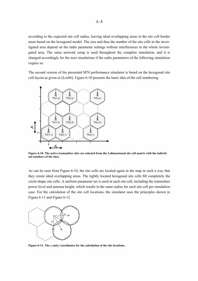
A–8

according to the expected site cell radius, leaving ideal overlapping areas in the site cell border areas based on the hexagonal model. The size and thus the number of the site cells in the inves-tigated area depend on the radio parameter settings without interferences in the whole investi-gated area. The same network setup is used throughout the complete simulation, and it is changed accordingly for the next simulations if the radio parameters of the following simulation require so.

The second version of the presented SFN performance simulator is based on the hexagonal site cell layout as given in [Lee86]. Figure 6-10 presents the basic idea of the cell numbering.

TX(1,1) TX(2,1) TX(x,1)

TX(x,2)TX(2,2)TX(1,2)

TX(1,y) TX(2,y) TX(x,y)

r

r

dx

dy

TX(1,1) TX(2,1) TX(x,1)

TX(x,2)TX(2,2)TX(1,2)

TX(1,y) TX(2,y) TX(x,y)

r

r

dx

dy

Figure 6-10. The active transmitter sites are selected from the 2-dimensional site cell matrix with the individ-ual numbers of the sites.

As can be seen from Figure 6-10, the site cells are located again in the map in such a way that they create ideal overlapping areas. The tightly located hexagonal site cells fill completely the circle-shape site cells. A uniform parameter set is used in each site cell, including the transmitter power level and antenna height, which results in the same radius for each site cell per simulation case. For the calculation of the site cell locations, the simulator uses the principles shown in Figure 6-11 and Figure 6-12.

rx

y

rx

y

Figure 6-11. The x and y coordinates for the calculation of the site locations.

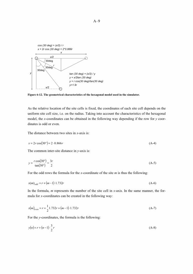
A–9

30deg

r30deg

x/2

cos (30 deg) = (x/2) / rx = 2r cos (30 deg) = 2*0.866r

x

y

x/2

30degtan (30 deg) = (x/2) / yy = x/2tan (30 deg)y = r cos(30 deg)/tan(30 deg)y=1.5r

Figure 6-12. The geometrical characteristics of the hexagonal model used in the simulator.

As the relative location of the site cells is fixed, the coordinates of each site cell depends on the uniform site cell size, i.e. on the radius. Taking into account the characteristics of the hexagonal model, the x-coordinates can be obtained in the following way depending if the row for y coor-dinates is odd or even.

The distance between two sites in x-axis is:

( ) rrx 866.0230cos2 ⋅=°= (A-4)

The common inter-site distance in y-axis is:

( )( ) 2

330tan30cos rry =

°°= (A-5)

For the odd rows the formula for the x-coordinate of the site m is thus the following:

( ) rmrmx odd 732.11)( ⋅−+= (A-6)

In the formula, m represents the number of the site cell in x-axis. In the same manner, the for-mula for x-coordinates can be created in the following way:

( ) ( ) rmrrmx even 732.11732.121 ⋅−++= (A-7)

For the y-coordinates, the formula is the following:

( ) ( ) rnrny231 ⋅−+= (A-8)

A–10

The simulations can be carried out for different site cell layouts. The symmetrical reuse pattern concept was selected for the simulations of Nsites=K sites presented in Publication IV. The reuse pattern size refers in this case to the SFN size, i.e. the site cells utilize the same frequency within the reuse patter size (unlike the original use of the SFN reuse patterns, e.g. in GSM fre-quency planning). Different SFN areas can thus be repeated by utilizing this pattern and by ap-plying different frequency for each SFN pattern, i.e. by utilising MFN for different SFN areas.

The term "SFN reuse pattern" is utilized to distinguish the idea from the original reuse pattern concept. Figure 6-13 clarifies the SFN reuse pattern concept.

Figure 6-13. The idea of the SFN reuse pattern. In this case, K=9. The colours represent different frequencies, each forming a single SFN area with 9 sites.

The most meaningful SFN reuse pattern size K can be obtained with the following formula by applying the TDMA reuse pattern concept [Lee86]:

kllkK −−= 2)( (A-9)

The variables k and l are positive integers with minimum value of 0. In the simulations, the SFN reuse pattern sizes of 1, 3, 4, 7, 9, 12, 16, 19 and 21 were used for the C/(N+I) distribution in order to obtain the carrier and interference distribution in both non-interfering and interfering networks (i.e. the presence of SER depends on the size of the SFN area). In this way, the lower values of K provides with the non-interfering SFN network until a limit that depends on the GI and FFT size parameters.

As a last step of the initial phase, the text files are named and the respective files are opened as a database for the writing of the results.

A–11

A.3 Simulation phase

Figure 6-14 shows the block diagram of the simulator in the simulation phase. Once the initialization of the simulator is done, the simulation rounds will be started. The simulations are repeated a total of 60,001 times by placing the DVB-H receiver in the investigated geographical area, calculating the total level of carriers and interferences in that spot. The value 60,001 is a result of the applied loop which is repeated from integer value of �30,000 to +30,000.

The first step is to initiate the random number generator. In this case, this is done by executing the only non-standard Pascal command of the simulator, i.e. “Randomize”. This provides the means to repeat the simulations with the same parameter values but with different locations of the receiver. As the round number of each complete simulation is sufficiently high, the final placement of the receiver is close to the uniform distribution over the whole area in x and y co-ordinates.

Next, all the relevant tables are cleaned by giving zero-values for all the table indexes. This guarantees that the values are stored and cumulated correctly even in the case of possible resid-ual values in the tables in the execution of the simulation.

Then, the DVB-H receiver is placed in the field by applying the random function. As the exact location in x/y coordinates of the sites is known from the initial phase of the code execution, as well as the height of the transmitter antennas (which is uniform in the basic version of the simulator, and can be given separately for each site in the 3rd version), the distance between the receiver and each one of the site antenna can be calculated in 3-dimensional space. These dis-tance objects are stored in respective tables during each simulation round. Furthermore, the re-spective path loss L can be calculated by applying the Okumura-Hata models that are coded in respective functions as sub programs. Furthermore, the long term and/or fast fading is added to this path loss value by using the respective cumulative presentations of the probability density functions created in the initial phase. As the simulator is snap-shot type, this is done separately for each location, i.e. in each simulation round.

It should be noted, that as the terminal can be located anywhere in the x/y-coordinates, the transmitter antenna height results in the minimum distance with the terminal as shown in Figure 6-15. If the terminal is relatively close to the site, the respective carrier could be higher than the upper scale limit of the C table (+50.0 dB). In such cases, the value is added to the table index C[500] representing the +50.0 dB value, or if that already contains 30,000 values (which is highly theoretical and not probable), the index C[499] representing the +49.9 dB value is in-creased respectively. This is due to the fact that the utilised Pascal compiler’s maximum integer value is limited to 32,000 unless possible longer integer values would be available and applied. This procedure assures that the cumulative presentation can be calculated correctly over the

A–12

whole area. Another solution would be to limit the minimum distance in x/y-coordinates be-tween the terminal and site sufficiently in order to limit the C value, but in this investigation it is not necessary. It should also be noted that the transmitter and receiver antennas are considered isotropic.

Initiate random generator.

Initiate the log files:Write headers with the parameter values.

Place the mobile randomly on the map.

Calculate the 3-D distance and path loss(taking into account fast and long term fadingand antenna gain) between the mobile and all

the TXs.

Initialization

Find nearest TX to the terminal as a reference.

Indicate if TXs are producing C or I (comparingeach one with the reference TX).

Calculate the dB level of C and I for each TX.

Finalization

Convert each C and I value from dB to absolutepower levels (W) and sum the total C and total

I. Convert the C and I back to dB values.

Write terminal’s x/y coordinates, C and I to file number 1.

Add C or I to cumulative tables.

Save cumulative results to log file number 2.

Are 60,001 rounds

complete?

Increase round counter by 1.

no

yes

Figure 6-14. The simulation phase.

A–13

x

y

z

x1

x2

y1 y2

z1

z2

DMS

Figure 6-15. The terminal is placed in the map varying the x and y coordinates, and the distance from the site antenna is calculated in 3D space.

The idea of the simulator is based on snap-shot analysis, i.e. the terminal is located on the map during each round without continuum from the previous round. If the distance between terminal and investigated site is less than the theoretical SFN limit shows, the signal is considered as use-ful carrier C, otherwise it is considered as interfering signal I. The effective distance Deff is used to decide weather the SFN limit is exceeded per site or if the terminal is within the SFN limits, i.e. it expresses the difference between the physical 3D distances of the arriving signals of the sites that are compared.

C1C2

C3

C4

C5

I1

I2

Effective SFN limit

Figure 6-16. The principle of the snap-shot of each simulation round.

The nearest site is identified and handled as a reference carrier C1. The comparison of the other sites, i.e. the effective distance that is the difference between the nearest site’s signal and the other one, is calculated. When the distance is within the maximum allowed SFN distance, i.e. when Deff � Dsfn, the respective carrier signal is taken into account if its level is more than the noise level, i.e. the sum of the noise floor and terminal noise figure. Equally, for the Deff > Dsfn, the interfering signal is taken into account only if it is greater than the sum of noise floor and terminal noise figure, in order to simplify the measurement procedure. The value for Dsfn is based on the initial values of FFT size and GI which together dictates the maximum allowed distance between the sites in non-interfering SFN. Figure 6-16 shows the basic principle of this idea. The distances between the terminal and each site are calculated separately as well as the

A–14

respective signal level of the investigated site. If the effective distance with the reference site is inside SFN, the signal component is considered as carrier, and otherwise it is considered as in-terference.

Now, all the relevant components of the carrier and interfering signals are summed in order to obtain the total level of C and I. This is done by converting the signal levels into absolute power levels and carrying out the summing, assuming that the signals are always non-coherent:

�=

=n

iitot CC

1

(A-10)

�=

=n

iitot II

1

(A-11)

In the formula, n represents the number of identified carriers, and m is the number of the inter-fering sources, per simulation round. After the summing, the value is again converted to the original presentation of received power level in dBm.

The total C and I of the simulation round is now stored into a text file with the respective infor-mation about the coordinates. It is also added into a cumulative C and I table, which in this case is an indexed table with index values of –500 to +500. If the C/N value is 12.5 dB, the value of the table index C[125] is increased by one. In this format, the C scale can thus be obtained di-rectly by observing the indexes, and the cumulative amount of the values per index is obtained by observing the respective value of the index. As can be noted, the raster of the indexed format is 0.1 dB. In cases when the C or I value is outside of the indexed range, the respective value is added to the extreme indexes (�500 or 500 presenting �50 dB and +50 dB and �499 or 499 pre-senting 49.9 dB) in order to maintain the statistical accuracy of the cumulative presentation.

When all the 60,001 simulation rounds have been executed, the text files are closed and the simulation ends.

A.4 Data analysis

The simulation model is based on the snap-shot principle, i.e. Monte-Carlo method. The re-ceiver is thus located on the field randomly, and the received total carrier power, as well as the possible received total interfering power, is calculated by taking into account the selected fading profile. The snap-shots are repeated until sufficient amount of samples has been collected.

A–15

The main outcome is the cumulative function of the occurred carrier levels within the simulated area, as well as interfering power levels. In this format, the percentage of the useful coverage area can be investigated directly by observing the dimensioned area location values.

The results are stored in a cumulative table which shows the CDF as such. Other option that is typically utilized in the coverage prediction of the planning tools like NetAct, would be to di-vide the area into relatively small sub-areas, e.g. 100 m × 100 m sized squares. The simulations can be repeated within each square in order to observe if the level of the carrier is above the minimum functional carrier threshold for more or equal percentage of the snap-shots compared to de designed area location probability value. If the level is high enough, the square is selected as a part of the functional coverage area.

This method presented in this thesis can also be utilized for the visual presentation of the cover-age area, but the principle is more suitable for the calculation of the CDF of the C/(N+I) distri-bution in a numerical format, taking into account each simulated point over the whole area. In any case, the simulator stores all the locations in x, y coordinates with the respective C and I values, so the post-processing to present the sub-region analysis would be possible. This was not done in these studies, though, as the visual presentation would not give added value for the presented C/(N+I) analysis.

As a result of the simulation, there are two files produced in plain text format, with the values separated by semi-commas. One file contains the entire C, I and location information of each simulation round, and the other one contains the C/N and I/N distribution in �50.0 dB…+50.0 dB scale. These tables can be post-processed in order to obtain the geographical distribution of the C and I levels (as shown in Publication VII), and the CDF and PDF of C/N, I/N and C/(N+I) curves as shown in Publications III, IV and, X.

The post-processing of the results was done by using MICROSOFT EXCEL. The respective text files can be imported to the EXCEL sheet by selecting the “;” as a separator.

The PDF of C and I distribution over the complete scale gives information about the presence and level of the carriers and interferences. If the whole area is within SFN, there are no I-com-ponents present whereas the extension of the SFN over its theoretical limits starts producing I components. The effect of parameter values like site antenna height and transmitter power levels on the interference levels can be thus investigated by repeating the complete simulations and varying the parameter values respectively. Publication III shows the antenna height and power level effects on the SFN interference level. In the second version of the simulator, the network layout can be designed by using SFN reuse patterns. Furthermore, the analysis can be limited into the coverage area of the used site cells. This gives possibility to compare the C/N and C/(N+I) distributions with different number of the used site cells. When multiple site cells are

A–16

compared with a single site cell, the effect of SFN gain can be investigated as shown in Publi-cation IV.

As an example about the interpretation of the results, the first log-file contains an individual simulation round’s x, y, total C and total I values in a single row. It is thus possible to make an additional analysis that plots the x and y coordinates when certain C, I, C/N and C/(N+I) criteria is achieved. This gives means of producing coverage maps that takes into account the balance of SFN gain and SFN interference as is presented in Publication IV.

The second log-file contains the C, I and C/(N+I) distribution in dB scale of �50...+50 dB. It is possible to present the C, I and C/(N+I) occurrences, e.g. in relative percentages over the whole scale as shown in Publication III. It is also possible to post-process the results in cumulative format, which gives the typical S-curves over the investigated area. In this way, it is possible to interpret the area outage or area location probabilities as a function of the C/(N+I) as shown in Publication III.

The idea is to investigate from the simulation results the cumulative C/(N+I) value that complies with the minimum percentage of the occurred events. This gives directly the area location prob-ability of the whole investigated area. If the area is not limited to the pre-calculated site cell ar-eas, the percentage shows the area location probability over the whole x/y-area. Otherwise, the results reflect the realistic situation of only site cells (including the overlapping proportion) in-cluded.

As for the interpretation of the results, Table 6-2 shows an example of the simulation that has been done by limiting the occurred events to the pre-calculated site cell area. This example re-fers to the second version of the simulator that uses the SFN reuse pattern sizes as a basis for creating the site cell areas. The related results are presented in deeper level in Publication IV by utilizing a more complete set of parameter values.

The reference site cell (K=1) represents the situation without SFN gain as only one radio path is present. When the simulation is done for larger SFN reuse pattern sizes, more radio paths are present. The total amount of carrier and interference components are summed, which makes it possible to obtain the SFN gain by comparing the results with wanted area location criteria. In this specific case, the radio parameters were: FFT=2K, GI=1/4, 16-QAM modulation, CR 1/2, MPE-FEC 1/2. The standard deviation value was selected to 5.5 and the location probability in the cell edge to 70 % which corresponds to 90 % area location probability. The height of the transmitter antenna was 60 meters, and the height of the terminal was 1.5 meters. The transmit-ter power level (EIRP) was +60 dBm. If we seek for the location area probability of 90% (which corresponds to 70% of area location probability in the site cell edge), it is now found as the 10% outage point of the results shown in Table 6-2.

A–17

Table 6-2. An example of simulation results, C/(N+I) as a function of the cumulative area location probability. A total of 7 complete simulations are presented, for the SFN reuse patterns K of 1, 3, 4, 7, 9, 12 and 16.

C/(I+N). dB K=1 K=3 K=4 K=7 K=9 K=12 K=16… … … … … … … …14 0.0871 0.0439 0.0375 0.0274 0.0377 0.05 0.0709

14.1 0.0894 0.0453 0.0397 0.0286 0.0391 0.0511 0.07214.2 0.0922 0.0473 0.0411 0.0296 0.0405 0.0521 0.073414.3 0.0947 0.0492 0.043 0.0314 0.0416 0.0532 0.074414.4 0.0973 0.0512 0.0448 0.0332 0.0433 0.0544 0.075614.5 0.0995 0.053 0.0466 0.0344 0.0447 0.0557 0.077214.6 0.1022 0.0552 0.0485 0.0361 0.0461 0.0572 0.078714.7 0.1049 0.057 0.0501 0.0375 0.0476 0.059 0.0814.8 0.1076 0.0591 0.052 0.0388 0.0495 0.0606 0.081514.9 0.1107 0.0612 0.0539 0.0403 0.0514 0.0621 0.083315 0.1137 0.0635 0.0557 0.0423 0.053 0.0635 0.0848

15.1 0.1162 0.0657 0.0579 0.0438 0.0548 0.0651 0.086615.2 0.1194 0.068 0.0602 0.0455 0.0565 0.0668 0.088515.3 0.123 0.0702 0.0622 0.0474 0.0581 0.0688 0.090315.4 0.1263 0.0729 0.0643 0.0491 0.0601 0.0707 0.09215.5 0.1294 0.0754 0.0665 0.0514 0.0618 0.0725 0.093915.6 0.133 0.078 0.0689 0.053 0.0636 0.0744 0.09615.7 0.1363 0.0808 0.0715 0.0545 0.0657 0.0762 0.09815.8 0.1394 0.0832 0.0738 0.0569 0.0677 0.0785 0.100315.9 0.1429 0.0858 0.0764 0.0592 0.0698 0.0805 0.102816 0.1467 0.0886 0.079 0.0614 0.0719 0.083 0.1051

16.1 0.1502 0.0916 0.0817 0.0638 0.0741 0.0854 0.107516.2 0.1537 0.0949 0.0847 0.0657 0.0765 0.0882 0.1116.3 0.1575 0.0978 0.0874 0.0681 0.0791 0.0907 0.112516.4 0.161 0.1007 0.0906 0.0708 0.0815 0.0933 0.115216.5 0.1645 0.1039 0.0936 0.0731 0.0836 0.0959 0.118216.6 0.1681 0.1069 0.0966 0.0757 0.0863 0.0982 0.120616.7 0.1721 0.1098 0.1 0.0787 0.0892 0.101 0.12316.8 0.1759 0.1128 0.1029 0.0813 0.0918 0.1034 0.125916.9 0.1796 0.1161 0.1059 0.084 0.0941 0.1065 0.128617 0.1834 0.1195 0.109 0.0876 0.0968 0.1095 0.1316

17.1 0.1872 0.1227 0.1123 0.0905 0.1001 0.1121 0.134517.2 0.1915 0.126 0.1155 0.0933 0.1027 0.1149 0.137317.3 0.1954 0.1295 0.1192 0.0966 0.1059 0.1176 0.140517.4 0.1992 0.1333 0.1228 0.0995 0.1089 0.1209 0.143617.5 0.2031 0.1369 0.1263 0.1025 0.112 0.124 0.146917.6 0.2072 0.1404 0.1298 0.106 0.115 0.1276 0.150317.7 0.2116 0.1446 0.134 0.1097 0.1183 0.1311 0.1538… … … … … … … …

When investigating the 10% area outage probability point, a clear tendency of SFN gain can be observed up to K=7 both in Table 6-2 and graphical presentation of it in Figure 6-17. Compared to the 1 site cell case which produces C/(N+I) of 14.5 dB 90 % of the locations, the area with

A–18

seven site cells produces C/(N+I) of 17.4 dB with the same 10% outage criteria. The SFN gain can thus be interpreted directly by comparing these values, resulting 17.4�14.5 dB = 2.9 dB. Then, as the number of sites grows, the SFN reuse pattern K=9 includes already part of the sites outside of the SFN area as the GI is not long enough for all the farthest sites.

It can be noted, though, that even the interference level produced via SFN reuse pattern size of K=16 of this example is still below the level that can be obtained via the SFN gain, so the bal-ance of SFN interferences and SFN gain is still positive. In fact, as presented in Publication IV, the SFN reuse pattern size of K=21 is still producing around 0 dB gain in this specific case, which indicates that the theoretical maximum SFN area, that would be clean of interferences, can be exceeded in a controlled way by utilizing the above mentioned parameter values.

SFN performance

0

0,02

0,04

0,06

0,08

0,1

0,12

0,14

0,16

0,18

0,2

11

11,5 12

12,5 13

13,5 14

14,5 15

15,5 16

16,5 17

17,5 18

dB

Out

age

prob

abili

ty

K=1K=3K=4K=7K=9K=12K=16

Figure 6-17. An amplified view to the outage probability of 10% (area location probability of 90 %) with respective C/(N+I) values for SFN reuse pattern size of K=1…16.

A.5 Functional analysis

The simulator locates the mobile terminal in the map according to the uniform distribution. If the location is not inside of any of the site cells, there is an option to discard those results. Nev-ertheless, all the occurred locations are saved to the log file. In both cases, the uniformity of the locations is important in order to have good cumulative presentation of the whole map. When the amount of the snap-shots is increased, also the accuracy of the results gets better.

A–19

A.5.1 Selection and reliability of the models

Propagation models

The major part of the simulations was based on the Okumura-Hata path loss prediction model [Hat80]. The model was selected for this thesis because it is relatively straightforward to im-plement in the simulator code as it is based on the formulas for each area type. The model is based on the practical measurements and mathematical modelling of the typical results. It fits to the simulations as in these cases there is no need to calculate the path loss in more detailed level, and its typical cell range is within the studied examples. The model can be assumed to provide sufficiently accurate results as it has been utilized widely as a basis in commercial net-work planning programs.

Also ITU-R P.1546-3 model was utilized in one of the cases to estimate the site cell coverage area in a large area due to the high mountain location. This model was selected because Oku-mura-Hata is not valid in the site area in question due to the much greater effective antenna height than Okumura-Hata supports. The ITU-R P.1546-3 model is more complicated to imple-ment in the simulator code as it is based on the curve mapping and interpolation and extrapola-tion of the curves. Nevertheless, as the case utilized only one value for the frequency and effec-tive antenna height, it was possible to create a mathematical formula by forming a regression curve. The accuracy of the produced formula is high enough for this case as the error margin analysis of A.5.2 shows. Also the model itself can be assumed to be enough accurate as indi-cated in [Öst06], which concluded that the model (its different variations) enhance the accuracy of the traditional models.

Simulator model

The simulations are based on the Monte-Carlo. It was selected as a base for the work because it suits well in the evaluation of the radio parameter effects over the whole investigated area. It is possible to take into account the channel types by including the effect of the path loss variations in a realistic yet relatively simple way. The model provides the possibility to investigate the in-ter-site effects on the power level contribution for both useful and interfering signals is possible to take into account in a large area that contains considerable amount of transmitters.

A typical solution of investigating the level of the coverage would be to divide the investigated area into small sub-regions, e.g. 100 m × 100 m to 500 m × 500 m squares. The cumulative dis-tribution of the signal level of each region can be investigated. If the area location probability criterion for the minimum C/N or C/(N+I) is fulfilled, the region can be marked as functional. Nevertheless, the simulator of this work was designed in such a way that the simulations were executed over the whole investigated area once by repeating 60,001 snap-shots per investigated parameter set. As Chapter A.5.3 and A.5.4 indicate, the accuracy of this method is sufficient for

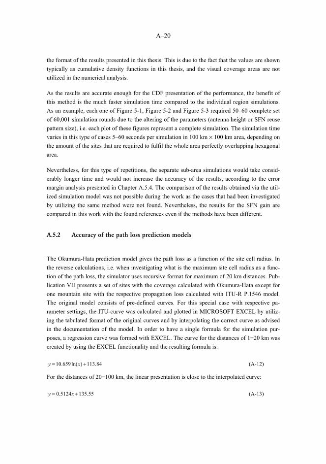
A–20

the format of the results presented in this thesis. This is due to the fact that the values are shown typically as cumulative density functions in this thesis, and the visual coverage areas are not utilized in the numerical analysis.

As the results are accurate enough for the CDF presentation of the performance, the benefit of this method is the much faster simulation time compared to the individual region simulations. As an example, each one of Figure 5-1, Figure 5-2 and Figure 5-3 required 50–60 complete set of 60,001 simulation rounds due to the altering of the parameters (antenna height or SFN reuse pattern size), i.e. each plot of these figures represent a complete simulation. The simulation time varies in this type of cases 5–60 seconds per simulation in 100 km × 100 km area, depending on the amount of the sites that are required to fulfil the whole area perfectly overlapping hexagonal area.

Nevertheless, for this type of repetitions, the separate sub-area simulations would take consid-erably longer time and would not increase the accuracy of the results, according to the error margin analysis presented in Chapter A.5.4. The comparison of the results obtained via the util-ized simulation model was not possible during the work as the cases that had been investigated by utilizing the same method were not found. Nevertheless, the results for the SFN gain are compared in this work with the found references even if the methods have been different.

A.5.2 Accuracy of the path loss prediction models

The Okumura-Hata prediction model gives the path loss as a function of the site cell radius. In the reverse calculations, i.e. when investigating what is the maximum site cell radius as a func-tion of the path loss, the simulator uses recursive format for maximum of 20 km distances. Pub-lication VII presents a set of sites with the coverage calculated with Okumura-Hata except for one mountain site with the respective propagation loss calculated with ITU-R P.1546 model. The original model consists of pre-defined curves. For this special case with respective pa-rameter settings, the ITU-curve was calculated and plotted in MICROSOFT EXCEL by utiliz-ing the tabulated format of the original curves and by interpolating the correct curve as advised in the documentation of the model. In order to have a single formula for the simulation pur-poses, a regression curve was formed with EXCEL. The curve for the distances of 1�20 km was created by using the EXCEL functionality and the resulting formula is:

84.113)ln(659.10 += xy (A-12)

For the distances of 20�100 km, the linear presentation is close to the interpolated curve:

55.1355124.0 += xy (A-13)

A–21

Path Loss 1-20 km y = 10,659Ln(x) + 113,84

110

115

120

125

130

135

140

145

150

1 2 3 4 5 6 7 8 9 10 11 12 13 14 15 16 17 18 19 20

Distance (km)

L (d

B)

600

860

1200

Figure 6-18. The formed curve for the distances of 1–20 km of the mountain site is close to the logarithmic form, as used in Publication VII.

Path Loss 1-20 km

140

145

150

155

160

165

170

175

180

185

190

20 30 40 50 60 70 80 90 100Distance (km)

L (d

B)

6008601200FSL

Figure 6-19. The interpolated curve for the distance of 20–100 km can be formed linearly.

The regression curves can now be obtained from. Figure 6-18 and Figure 6-19 show the values obtained by interpolating the tabulated values of the report ITU-R P.1546-3, and the values that can be obtained from the above mentioned regression curves.

A–22

Difference of trend line and original values

-1.0

-0.8

-0.6

-0.4

-0.2

0.0

0.2

0.4

0.6

0.8

1.01 2 3 4 5 6 7 8 9 10 11 12 13 14 15 16 17 18 19 20 30 40 50 60 70 80 90 100

Distance (km)

Diff

(reg

ress

ion

- orig

inal

)

Figure 6-20. The error margin of the estimated path loss values obtained via the original tabulated values of the model ITU-R P.1546-3 and the respective regression curves is within +0.2…–0.5 dB up to 60 km of dis-tance. There is also a peak up to +0.8 dB in close distance which does not have significance in this case. Table 6-3. Comparison of the values obtained by interpolating the tabulated form and the regression curves.

d L_860m_regr L_860m_orig Diff reg_orig1 113.84 112.99 0.82 121.23 121.61 -0.43 125.55 125.97 -0.44 128.62 128.96 -0.35 130.99 131.24 -0.26 132.94 133.10 -0.27 134.58 134.66 -0.18 136.00 136.02 0.09 137.26 137.23 0.0

10 138.38 138.31 0.111 139.40 139.30 0.112 140.33 140.21 0.113 141.18 141.05 0.114 141.97 141.84 0.115 142.71 142.58 0.116 143.39 143.29 0.117 144.04 143.96 0.118 144.65 144.61 0.019 145.22 145.24 0.020 145.77 145.84 -0.130 150.92 151.24 -0.340 156.05 156.28 -0.250 161.17 161.46 -0.360 166.29 166.84 -0.570 171.42 172.23 -0.880 176.54 177.44 -0.990 181.67 182.31 -0.6

100 186.79 186.81 0.0

A–23

Now, an analysis for the difference of the values shown in Table 6-3 can be obtained as shown in Figure 6-20. As can be noted from Figure 6-20, the difference between the estimated path loss value of the original tabulated values and the values that can be calculated with the regres-sion curves is not significant in this type of simulations.

A.5.3 Uniformity of the locations

In order to evaluate the level of uniformity when the terminal is located on the map, the given area can be divided into smaller pieces in x and y coordinates. In a uniform 2D area, the distri-bution of the MS locations should occur approximately equally in each slice of these sub-areas.

Let us select an example of 100×100 km area with sufficient amount of sites. The parameters for this test are: base station antenna height 100 m, MS height 1.5 m, MS antenna gain �7 dBi, frequency 700 MHz, standard deviation 5.5 dB, TX power +70 dBm, Rayleigh fading not selected, large-scale fading on, location probability 90 %, small and medium city type, bandwidth 8 MHz, modulation QPSK, code rate 1/2, MPE-FEC rate 2/3, guard interval 1/4, FFT mode 8K.

This parameter set creates a hexagonal site cell layout with maximum path loss of 148.1 dB, site cell radius of 10.0 km (i.e. where the carrier is still above the minimum C/N of 8.5 dB), maxi-mum interference path loss 156.6 dB and corresponding interfering site cell radius of 18.5 km (i.e. distance where the interfering signal is still above the noise floor). The total number of transmitter sites in that area is 33, with carrier to interfering site cells proportion of 3.5 (taking into account all the sites even if the interfering signal would be less than noise floor, i.e. there are total of 410 links from which interfering links are 118).

Let’s carry out a complete simulation round and consider the distribution of the MS location by post-processing the location information. We can divide the area into 10 km slices both in x and y axis as shown in Figure 6-21 and investigate, what is the percentage of the occurred locations in each one of the squares. In the ideal case, each slice should contain 10 % of the total occurred events in x-axis, and 10 % per slice in y-axis. The total amount of simulation rounds and thus location results is 60,001 in this revision.

As can be seen from Table 6-4 and Table 6-5, the standard deviation between the 10 slices per simulation round is typically about 0.10�0.17 %. Figure 6-22 shows also in graphical format the distribution of the occurred locations for x and y coordinates. Each slice of the figures represents 10 % of the geographical area.

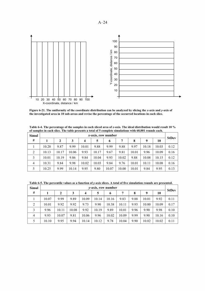
A–24

10 20 30 40 50 60 70 80 90 100X-coordinate, distance / km

10

20

30

40

50

60

70

80

90

100

Y-co

ordi

nate

, dis

tanc

e/ k

m

Figure 6-21. The uniformity of the coordinate distribution can be analyzed by slicing the x-axis and y-axis of the investigated area in 10 sub-areas and revise the percentage of the occurred locations in each slice.

Table 6-4. The percentage of the samples in each sliced area of x-axis. The ideal distribution would result 10 % of samples in each slice. The table presents a total of 5 complete simulations with 60,001 rounds each.

x-axis, row number Simul # 1 2 3 4 5 6 7 8 9 10

StDev

1 10.20 9.87 9.99 10.01 9.88 9.99 9.88 9.97 10.18 10.03 0.12 2 10.13 10.17 10.06 9.93 10.17 9.67 9.81 10.01 9.96 10.09 0.16 3 10.01 10.19 9.86 9.84 10.04 9.93 10.02 9.88 10.08 10.15 0.12 4 10.31 9.84 9.98 10.02 10.03 9.84 9.76 10.01 10.11 10.08 0.16 5 10.25 9.99 10.14 9.95 9.80 10.07 10.00 10.01 9.84 9.95 0.13

Table 6-5. The percentile values as a function of y-axis slices. A total of five simulation rounds are presented. y-axis, row number Simul

# 1 2 3 4 5 6 7 8 9 10 StDev

1 10.07 9.99 9.89 10.09 10.14 10.16 9.83 9.88 10.01 9.92 0.11 2 10.01 9.92 9.92 9.73 9.90 10.38 10.11 9.93 10.00 10.09 0.17 3 9.96 10.11 10.08 9.92 10.19 9.89 10.01 9.96 9.90 9.98 0.10 4 9.93 10.07 9.81 10.06 9.96 10.02 10.09 9.99 9.90 10.16 0.10 5 10.10 9.95 9.94 10.14 10.12 9.78 10.04 9.90 10.02 10.02 0.11

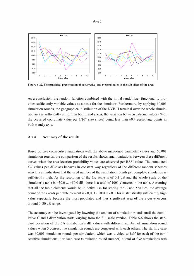
A–25

X-axis

9,60

9,70

9,80

9,90

10,00

10,10

10,20

10,30

10,40

1 2 3 4 5 6 7 8 9 10X-axis slice

Y-axis

9,60

9,70

9,80

9,90

10,00

10,10

10,20

10,30

10,40

10,50

1 2 3 4 5 6 7 8 9 10y-axis slice

Figure 6-22. The graphical presentation of occurred x- and y-coordinates in the sub-slices of the area.

As a conclusion, the random function combined with the initial randomizer functionality pro-vides sufficiently variable values as a basis for the simulator. Furthermore, by applying 60,001 simulation rounds, the geographical distribution of the DVB-H terminal over the whole simula-tion area is sufficiently uniform in both x and y axis, the variation between extreme values (% of the occurred coordinate value per 1/10th size slices) being less than ±0.4 percentage points in both x and y axis.

A.5.4 Accuracy of the results

Based on five consecutive simulations with the above mentioned parameter values and 60,001 simulation rounds, the comparison of the results shows small variations between these different curves when the area location probability values are observed per RSSI value. The cumulated C/I values per dB-class behaves in constant way regardless of the different random schemes which is an indication that the used number of the simulation rounds per complete simulation is sufficiently high. As the resolution of the C/I scale is of 0.1 dB and the whole scale of the simulator’s table is �50.0 ... +50.0 dB, there is a total of 1001 elements in the table. Assuming that all the table elements would be in active use for storing the C and I values, the average count of the events per table element is 60,001 / 1001 = 60. This is statistically sufficiently high value especially because the most populated and thus significant area of the S-curve occurs around 0–30 dB range.

The accuracy can be investigated by lowering the amount of simulation rounds until the cumu-lative C and I distribution starts varying from the full scale version. Table 6-6 shows the stan-dard deviation of the C/I distribution’s dB values with different number of simulation round values when 5 consecutive simulation rounds are compared with each others. The starting case was 60,001 simulation rounds per simulation, which was divided to half for each of the con-secutive simulations. For each case (simulation round number) a total of five simulations was

A–26

carried out. The respective maximum and minimum values was investigated in 8.5 dB point in order to see the variations of the results in probability % scale. The respective results are shown in Table 6-6. Secondly, the C/(N+I) value variation in 5% point of probability scale was ob-served to see the effect in dB values. The results are presented in Table 6-7.

Table 6-6. The analysis of probability variations when C/I = 8.5 dB reference point is observed in each simula-tion. Table shows the respective variations in probability values.

Rounds per simulation

Probability for C/I point (8.5 dB), Min

Probability for C/I point (8.5 dB), Max

Difference of probabilities,

max-min, % unit

Average Std

60,001 4.25 4.34 0.09 4.31 0.04 30,000 4.27 4.55 0.28 4.36 0.12 15,000 3.87 4.35 0.48 4.12 0.17 7,500 4.00 4.40 0.40 4.18 0.16 3,750 4.05 4.72 0.67 4.39 0.26 1,875 4.00 4.53 0.53 4.22 0.20

Table 6-7. The analysis of the variations of the interpretation of C/I value when 5% probability point is ob-served.

Rounds per simulation

C/I for prob. point (5%),

Min

C/I for prob. point (5%),

Max

Difference of C/I, max-min,

dB

Average Std

60,001 9.3 9.6 0.3 9.46 0.11 30,000 9.1 9.6 0.5 9.38 0.18 15,000 9.4 10.0 0.6 9.72 0.23 7,500 9.2 9.9 0.7 9.68 0.28 3,750 8.9 9.6 0.7 9.32 0.28 1,875 9.1 10.1 1.0 9.58 0.45

Figure 6-23 shows the effect of the number of the simulation rounds on the accuracy of the re-sults. When observing the cumulative distribution curve in the most typical C/I range, i.e. ap-proximately in the minimum threshold area for the QPSK and 16-QAM cases, the effect can be seen clearly in visual format. It can be noted that 60,001 simulation rounds produces smooth and constant curves, i.e. their variance is sufficiently low in order to interpret the C/I and prob-ability mapping in sufficiently accurate way.

By considering Figure 6-23, and more specifically the 5 % criteria, Table 6-8 can be created to indicate the variance of the results of each case.

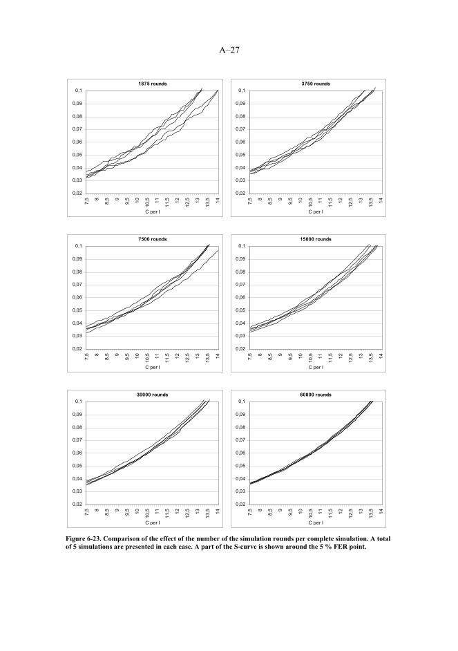
A–27

1875 rounds

0,02

0,03

0,04

0,05

0,06

0,07

0,08

0,09

0,17,

5 8

8,5 9

9,5 10

10,5 11

11,5 12

12,5 13

13,5 14

C per I

3750 rounds

0,02

0,03

0,04

0,05

0,06

0,07

0,08

0,09

0,1

7,5 8

8,5 9

9,5 10

10,5 11

11,5 12

12,5 13

13,5 14

C per I

7500 rounds

0,02

0,03

0,04

0,05

0,06

0,07

0,08

0,09

0,1

7,5 8

8,5 9

9,5 10

10,5 11

11,5 12

12,5 13

13,5 14

C per I

15000 rounds

0,02

0,03

0,04

0,05

0,06

0,07

0,08

0,09

0,17,

5 8

8,5 9

9,5 10

10,5 11

11,5 12

12,5 13

13,5 14

C per I

30000 rounds

0,02

0,03

0,04

0,05

0,06

0,07

0,08

0,09

0,1

7,5 8

8,5 9

9,5 10

10,5 11

11,5 12

12,5 13

13,5 14

C per I

60000 rounds

0,02

0,03

0,04

0,05

0,06

0,07

0,08

0,09

0,1

7,5 8

8,5 9

9,5 10

10,5 11

11,5 12

12,5 13

13,5 14

C per I

Figure 6-23. Comparison of the effect of the number of the simulation rounds per complete simulation. A total of 5 simulations are presented in each case. A part of the S-curve is shown around the 5 % FER point.

A–28

Table 6-8. The accuracy analysis of the simulation cases.

Rounds PTX(1) PTX(2) PTX(3) PTX(4) PTX(5) x Diff

(min - max)

Std

1,875 9.05 9.25 9.40 10.05 10.10 9.57 1.05 0.48 3,750 8.90 9.20 9.40 9.45 9.60 9.31 0.70 0.27 7,500 9.20 9.70 9.80 9.80 8.85 9.47 0.95 0.43

15,000 9.40 9.60 9.75 9.85 10.05 9.73 0.65 0.25 30,000 9.00 9.35 9.45 9.45 9.55 9.36 0.55 0.21 60,001 9.30 9.45 9.45 9.50 9.55 9.45 0.25 0.09

The analysis can be still done more detailed by observing the cumulative histogram of the stan-dard deviation values as a function of the number of simulation rounds. In this analysis, the standard deviation of five consecutive simulations is observed for each dB category, and the standard deviation values is collected as a histogram with the resolution of 0.001 (i.e. with 0.1% resolution of the probability).

Cumulative Standard Deviation (resolution 0.001)

40,00

50,00

60,00

70,00

80,00

90,00

100,00

0..0

.001

0.00

1-0.

002

0.00

2-0.

003

0.00

3-0.

004

0.00

4-0.

005

0.00

5-0.

006

0.00

6-0.

007

0.00

7-0.

008

0.00

8-0.

009

0.00

9-0.

010

0.01

0-0.

011

0.01

1-0.

012

0.01

2-0.

013

0.01

3-0.

014

0.01

4-0.

015

60001 rounds

30000 rounds

15000 rounds

7500 rounds

3750 rounds

1875 rounds

Figure 6-24. Cumulative presentation of the standard deviation classes per different lengths of the simulation.

As can be observed from Figure 6-23, the five simulation results of 60,001-round case provides a good correlation and thus accuracy, 75 % of the standard deviation values being maximum 0.1 %, and all the results being within 0.4 %. Also 30,000 and 15,000 simulation rounds would pro-

A–29

vide an accuracy of 0.5 % in probability scale whilst the 7,500 and 3,750 rounds provides about 0.9 % accuracy, and 1875 rounds less than 1.5 %.

As a conclusion, 60,001 simulation rounds provide sufficient accuracy for the simulation re-sults. It can be assumed that higher number does not increase the accuracy considerably in prac-tical interpretations of the performance; Table 6-6 shows that the maximum error in interpreta-tion of the dB values in typical probability range is about 0.3 dB. With typical CPU power the complete simulation with 60,001 rounds takes only few minutes in the most demanding cases presented in this thesis. Furthermore, the amount of data is still manageable with typical post processing software that might limit the maximum row number to about 65,000.

It can be estimated that the reliability of the results is sufficiently high for the presented exam-ples in the radio propagation level simulations. This claim is based on the assumption that the higher protocol layers are functioning ideally.

Appendix B Publications

B.1 Radio network planning studies

The main contribution of this thesis for the general radio network planning area is presented in Publications I, V and VI.

Publication I contains the investigations of the balancing of the site parameters and network costs. The objective of this part was to create a method that can be used as an iterative element in the cost-efficient network planning process. Publication I also presents selected case exam-ples how the optimal cost can be obtained in SFN area. This publication clarifies the topic be-cause the CAPEX and OPEX optimisation of the DVB-H networks analysis as a function of the radio network planning parameters was not found in the presented way by the publication of the study.

Publication V clarifies the DVB-H radio network coverage planning principles in a dense urban area with selected case examples. It shows the useful coverage areas when the parameters are selected in such a way that they do not create SFN interference in the investigated area. Based on this study, the importance of the radio propagation model adjustment is shown. It is also proved that the basic theoretical prediction models can be applied in the initial phase of the net-work planning with a sufficiently good correlation with the more advanced coverage tools. These results can be used as a basis for the investigation of the effects of the parameter value variations, i.e. when the sites start to cause interferences. Publication VII shows the related in-terference analysis via simulations. As the service area is the same, Publications V and VII can be used as a pair for a coverage and interference analysis in a realistic urban network. The stud-ies presented in this thesis show the estimated interference behaviour.

The radiation of the DVB-H transmitter site can be limiting factor, which should be taken into account in all phases of the radio network planning and site selection process. Publication VI presents the analysis of EMC and human exposure limits of DVB-H transmitter sites. The method and related case results might move the optimal power level that is derived from the radio link budget, and might result a need for modifications of the initially planned transmitter and antenna types. The general safety zone calculations of mobile and broadcast networks can be found in various sources, but these case studies were done especially for DVB-H in order to complete the radio network process.

B.2 Field measurement methodology

In order to assure the required quality level of the DVB-H radio network, it is essential to carry out field measurements as a basis for the network fine-tuning. The field measurement related studies with new analysis method are presented in Publications II, VIII, IX and XI.

Publication II, and its extended version in Publication IX, shows a method that can be applied for the fast revisions of the network performance with respective data collection, post-process-ing and analysis. The case examples and their results of the Publications show the importance of the parameter adjustment as a function of the radio channel type in outdoor environment. The presented method for the post-processing of the measurement data as well as for the respective analysis and case results are based on the already published data collection software of the DVB-H terminals. The post-processing method and the analysis gives additional value, e.g. for the WingTV field measurement documentation [Bou06], [Apa06a] and [Apa06b] which clari-fies the planning process of the DVB-H radio network. This thesis also analyses the accuracy of the presented measurement method of MPE-FEC gain in more detailed level compared to the principles presented in [Dvb06] and [Dvb09].

Publication VIII continues from the previous studies and shows the field measurement method, post-processing and analysis with respective results in indoor and outdoor environments. In ad-dition to the methodology, the results indicate the logical set of values for the error correction related parameters which extend the results obtained in [Apa06a] and [Apa06b].

B.3 Simulation methodology

A DVB-H radio performance simulator was developed for carrying out analysis of the Single Frequency Network (SFN) aspects. The summary of the principle and functionality of the simulator is presented in Appendix A. The simulation based studies are used in Publications III, IV, VII and X.

Publication III presents a principle that can be applied for the simulations of the interference levels in over-sized SFN area. The results show the effect of the antenna height and transmitter power level on the error rate. The simulation method can be used for the estimation of the se-verity of the errors, and it provides information about the optimal setting of the antenna heights and transmitter power levels that still fulfils the final radio reception quality requirement even if the theoretical SFN limits are exceeded. The simulator is based on the geographical area that is filled with uniformly distributed cells.

Publication IV shows the further development of the above mentioned simulator. It is based on the SFN reuse patterns of the transmitters that define the number of the transmitters in the SFN area. This method gives means for estimating the SFN gain as a function of the number of the transmitter sites and their radio parameters. The SFN area can also be extended, and the simula-tion results show the effect of the increased SFN interference levels. The results can be used in order to balance the SFN gain and interference level, which is useful in the selection of the re-lated radio parameter values in the radio network planning process.

Publication VII presents a further development of the above mentioned simulation principles. It shows that the basic idea can be applied also in the practical environment by setting the site spe-cific location, antenna height and transmitter power level. It also combines two propagation prediction models, i.e. Okumura-Hata for the basic sites and ITU-R P.1546-3 for large coverage sites. The simulations show the distribution of the carrier and interferences as a function of the radio parameter values in a real urban environment. The simulation results can be used for the estimation of the relation between the realistic coverage obtained in Publication VII and the SFN interference levels that are caused by the radio parameter adjustment.

Publication X is an extended version of Publication IV, and it compiles the presentations of the simulator in the Publications III, IV and VII.

9HSTFMG*aeaaia+

ISBN: 978-952-60-4009-7 (pdf) ISBN: 978-952-60-4008-0 ISSN-L: 1799-4934 ISSN: 1799-4942 (pdf) ISSN: 1799-4934 Aalto University

Department of Communications and Networking aalto.fi

BUSINESS + ECONOMY ART + DESIGN + ARCHITECTURE SCIENCE + TECHNOLOGY CROSSOVER DOCTORAL DISSERTATIONS

Aalto-D

D 4

/2011

The aim of this doctoral dissertation is to investigate advanced DVB-H radio network planning and optimisation. This dissertation presents the results of measurement techniques, network coverage and quality estimation, technological and economical optimisation, as well as error correction and single frequency network performance. The outcome includes proposed DVB-H radio network planning and optimisation methods that can be applied to the further investigation of detailed parameters in the radio link budget. There are also case studies that show the functionality of the presented methods with typical performance values.

Jyrki T. J. Penttinen T

he Planning and Optim

isation of DV

B-H

Radio N

etwork

Aalto

Unive

rsity

Department of Communications and Networking

The Planning and Optimisation of DVB-H Radio Network

Jyrki T. J. Penttinen

DOCTORAL DISSERTATIONS

School of Electrical Engineering

Date post:	09-Apr-2018
Category:	Documents
Upload:	phungdieu
View:	216 times
Download:	3 times

The Planning and Optimisation of DVB-H Radio...

Documents