The Positive Grassmannian, scattering amplitudes, and soliton solutions to the KP equation Lauren K. Williams, UC Berkeley Lauren K. Williams (UC Berkeley) The Positive Grassmannians April 2015 1 / 24
Transcript
The Positive Grassmannian,
scattering amplitudes, and soliton solutions to the KPequation
Lauren K. Williams, UC Berkeley
Lauren K. Williams (UC Berkeley) The Positive Grassmannians April 2015 1 / 24
Open problem
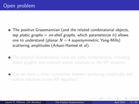
The positive Grassmannian (and the related combinatorial objects,esp plabic graphs = on-shell graphs, which parameterize it) allowsone to understand (planar N = 4 supersymmetric Yang-Mills)scattering amplitudes (Arkani-Hamed et al).
The positive Grassmannian (and the same combinatorics, includingplabic graphs) also controls soliton solutions to the KP equation.
Can we make a direct connection between scattering amplitudes andsoliton solutions to the KP equation?
Lauren K. Williams (UC Berkeley) The Positive Grassmannians April 2015 2 / 24
Open problem
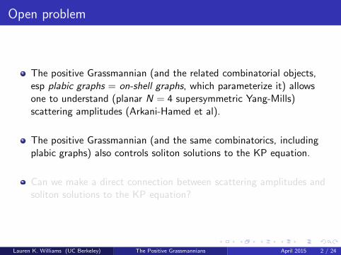
The positive Grassmannian (and the related combinatorial objects,esp plabic graphs = on-shell graphs, which parameterize it) allowsone to understand (planar N = 4 supersymmetric Yang-Mills)scattering amplitudes (Arkani-Hamed et al).
The positive Grassmannian (and the same combinatorics, includingplabic graphs) also controls soliton solutions to the KP equation.
Can we make a direct connection between scattering amplitudes andsoliton solutions to the KP equation?
Lauren K. Williams (UC Berkeley) The Positive Grassmannians April 2015 2 / 24
Open problem
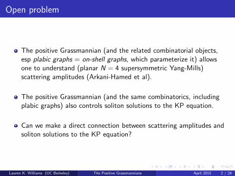
The positive Grassmannian (and the related combinatorial objects,esp plabic graphs = on-shell graphs, which parameterize it) allowsone to understand (planar N = 4 supersymmetric Yang-Mills)scattering amplitudes (Arkani-Hamed et al).
The positive Grassmannian (and the same combinatorics, includingplabic graphs) also controls soliton solutions to the KP equation.
Can we make a direct connection between scattering amplitudes andsoliton solutions to the KP equation?
Lauren K. Williams (UC Berkeley) The Positive Grassmannians April 2015 2 / 24
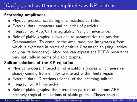
(Grkn)≥0, and scattering amplitudes vs KP solitons
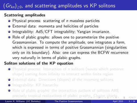
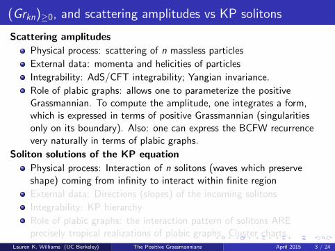
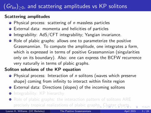
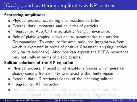
Scattering amplitudes
Physical process: scattering of n massless particles
External data: momenta and helicities of particles
Role of plabic graphs: allows one to parameterize the positiveGrassmannian. To compute the amplitude, one integrates a form,which is expressed in terms of positive Grassmannian (singularitiesonly on its boundary). Also: one can express the BCFW recurrencevery naturally in terms of plabic graphs.
Soliton solutions of the KP equation
Physical process: Interaction of n solitons (waves which preserveshape) coming from infinity to interact within finite region
External data: Directions (slopes) of the incoming solitons
Integrability: KP hierarchy
Role of plabic graphs: the interaction pattern of solitons AREprecisely tropical realizations of plabic graphs. Cluster charts.
Lauren K. Williams (UC Berkeley) The Positive Grassmannians April 2015 3 / 24
(Grkn)≥0, and scattering amplitudes vs KP solitons
Scattering amplitudes
Physical process: scattering of n massless particles
External data: momenta and helicities of particles
Role of plabic graphs: allows one to parameterize the positiveGrassmannian. To compute the amplitude, one integrates a form,which is expressed in terms of positive Grassmannian (singularitiesonly on its boundary). Also: one can express the BCFW recurrencevery naturally in terms of plabic graphs.
Soliton solutions of the KP equation
Physical process: Interaction of n solitons (waves which preserveshape) coming from infinity to interact within finite region
External data: Directions (slopes) of the incoming solitons
Integrability: KP hierarchy
Role of plabic graphs: the interaction pattern of solitons AREprecisely tropical realizations of plabic graphs. Cluster charts.
Lauren K. Williams (UC Berkeley) The Positive Grassmannians April 2015 3 / 24
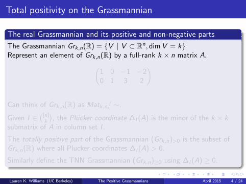
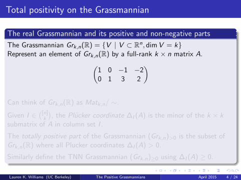
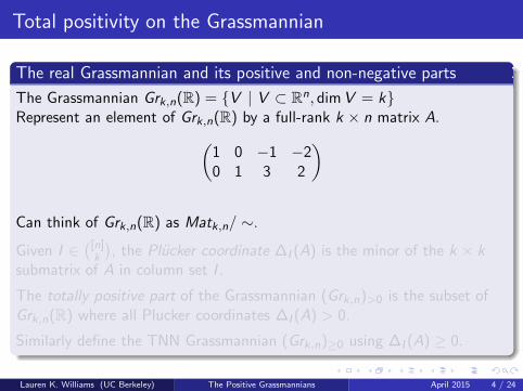
Total positivity on the Grassmannian
The real Grassmannian and its positive and non-negative parts
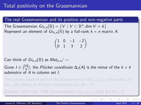
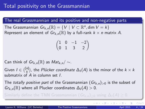
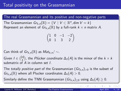
The Grassmannian Grk,n(R) = {V | V ⊂ Rn, dimV = k}
Represent an element of Grk,n(R) by a full-rank k × n matrix A.
(
1 0 −1 −20 1 3 2
)
Can think of Grk,n(R) as Matk,n/ ∼.
Given I ∈([n]k
)
, the Plucker coordinate ∆I (A) is the minor of the k × ksubmatrix of A in column set I .
The totally positive part of the Grassmannian (Grk,n)>0 is the subset ofGrk,n(R) where all Plucker coordinates ∆I (A) > 0.
Similarly define the TNN Grassmannian (Grk,n)≥0 using ∆I (A) ≥ 0.
Lauren K. Williams (UC Berkeley) The Positive Grassmannians April 2015 4 / 24
Total positivity on the Grassmannian
The real Grassmannian and its positive and non-negative parts
The Grassmannian Grk,n(R) = {V | V ⊂ Rn, dimV = k}
Represent an element of Grk,n(R) by a full-rank k × n matrix A.
(
1 0 −1 −20 1 3 2
)
Can think of Grk,n(R) as Matk,n/ ∼.
Given I ∈([n]k
)
, the Plucker coordinate ∆I (A) is the minor of the k × ksubmatrix of A in column set I .
The totally positive part of the Grassmannian (Grk,n)>0 is the subset ofGrk,n(R) where all Plucker coordinates ∆I (A) > 0.
Similarly define the TNN Grassmannian (Grk,n)≥0 using ∆I (A) ≥ 0.
Lauren K. Williams (UC Berkeley) The Positive Grassmannians April 2015 4 / 24
Postnikov’s decomposition of (Grk ,n)≥0 into positroid cells
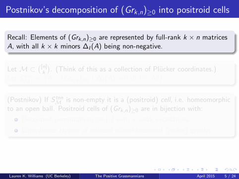
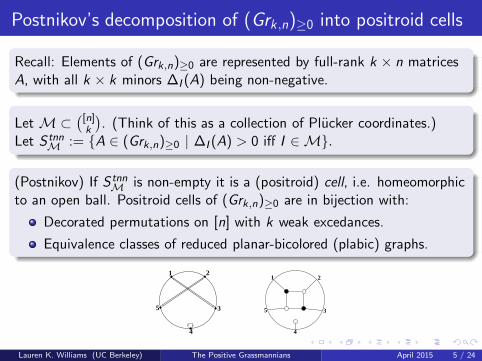
Recall: Elements of (Grk,n)≥0 are represented by full-rank k × n matricesA, with all k × k minors ∆I (A) being non-negative.
Let M ⊂([n]k
)
. (Think of this as a collection of Plucker coordinates.)Let S tnn
M := {A ∈ (Grk,n)≥0 | ∆I (A) > 0 iff I ∈ M}.
(Postnikov) If S tnnM is non-empty it is a (positroid) cell, i.e. homeomorphic
to an open ball. Positroid cells of (Grk,n)≥0 are in bijection with:
Decorated permutations on [n] with k weak excedances.
Equivalence classes of reduced planar-bicolored (plabic) graphs.
Lauren K. Williams (UC Berkeley) The Positive Grassmannians April 2015 5 / 24
Postnikov’s decomposition of (Grk ,n)≥0 into positroid cells
Recall: Elements of (Grk,n)≥0 are represented by full-rank k × n matricesA, with all k × k minors ∆I (A) being non-negative.
Let M ⊂([n]k
)
. (Think of this as a collection of Plucker coordinates.)Let S tnn
M := {A ∈ (Grk,n)≥0 | ∆I (A) > 0 iff I ∈ M}.
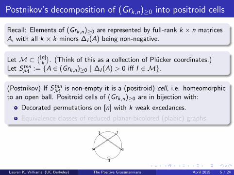
(Postnikov) If S tnnM is non-empty it is a (positroid) cell, i.e. homeomorphic
to an open ball. Positroid cells of (Grk,n)≥0 are in bijection with:
Decorated permutations on [n] with k weak excedances.
Equivalence classes of reduced planar-bicolored (plabic) graphs.
1 2
3
4
5
Lauren K. Williams (UC Berkeley) The Positive Grassmannians April 2015 5 / 24
Postnikov’s decomposition of (Grk ,n)≥0 into positroid cells
Recall: Elements of (Grk,n)≥0 are represented by full-rank k × n matricesA, with all k × k minors ∆I (A) being non-negative.
Let M ⊂([n]k
)
. (Think of this as a collection of Plucker coordinates.)Let S tnn
M := {A ∈ (Grk,n)≥0 | ∆I (A) > 0 iff I ∈ M}.
(Postnikov) If S tnnM is non-empty it is a (positroid) cell, i.e. homeomorphic
to an open ball. Positroid cells of (Grk,n)≥0 are in bijection with:
Decorated permutations on [n] with k weak excedances.
Equivalence classes of reduced planar-bicolored (plabic) graphs.
1 2
3
4
5
1 2
3
4
5
Lauren K. Williams (UC Berkeley) The Positive Grassmannians April 2015 5 / 24
The interaction of shallow water waves
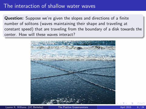
Question: Suppose we’re given the slopes and directions of a finitenumber of solitons (waves maintaining their shape and traveling atconstant speed) that are traveling from the boundary of a disk towards thecenter. How will these waves interact?
Lauren K. Williams (UC Berkeley) The Positive Grassmannians April 2015 6 / 24
The interaction of shallow water waves
Question: Suppose we’re given the slopes and directions of a finitenumber of solitons (waves maintaining their shape and traveling atconstant speed) that are traveling from the boundary of a disk towards thecenter. How will these waves interact?
Lauren K. Williams (UC Berkeley) The Positive Grassmannians April 2015 6 / 24
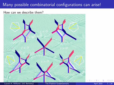
Many possible combinatorial configurations can arise!
How can we describe them?
Lauren K. Williams (UC Berkeley) The Positive Grassmannians April 2015 7 / 24
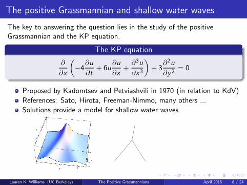
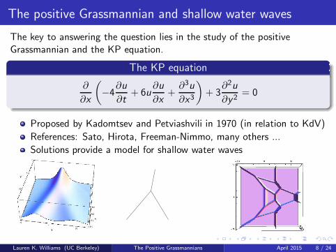
The positive Grassmannian and shallow water waves
The key to answering the question lies in the study of the positiveGrassmannian and the KP equation.
The KP equation
∂
∂x
(
−4∂u
∂t+ 6u
∂u
∂x+
∂3u
∂x3
)
+ 3∂2u
∂y2= 0
Proposed by Kadomtsev and Petviashvili in 1970 (in relation to KdV)
References: Sato, Hirota, Freeman-Nimmo, many others ...
Solutions provide a model for shallow water waves
Lauren K. Williams (UC Berkeley) The Positive Grassmannians April 2015 8 / 24
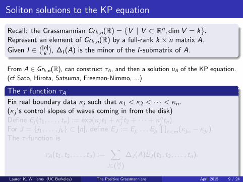
Soliton solutions to the KP equation
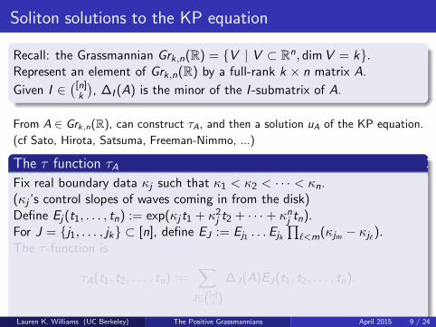
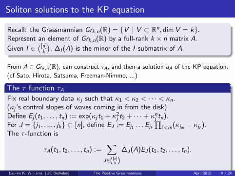
Recall: the Grassmannian Grk,n(R) = {V | V ⊂ Rn, dimV = k}.
Represent an element of Grk,n(R) by a full-rank k × n matrix A.
Given I ∈([n]k
)
, ∆I (A) is the minor of the I -submatrix of A.
From A ∈ Grk,n(R), can construct τA, and then a solution uA of the KP equation.
(cf Sato, Hirota, Satsuma, Freeman-Nimmo, ...)
The τ function τA
Fix real boundary data κj such that κ1 < κ2 < · · · < κn.(κj ’s control slopes of waves coming in from the disk)Define Ej (t1, . . . , tn) := exp(κj t1 + κ2j t2 + · · · + κnj tn).For J = {j1, . . . , jk} ⊂ [n], define EJ := Ej1 . . .Ejk
∏
ℓ<m(κjm − κjℓ).The τ -function is
τA(t1, t2, . . . , tn) :=∑
J∈([n]k )
∆J(A)EJ (t1, t2, . . . , tn).
Lauren K. Williams (UC Berkeley) The Positive Grassmannians April 2015 9 / 24
Soliton solutions to the KP equation
The τ function τA
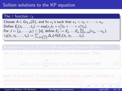
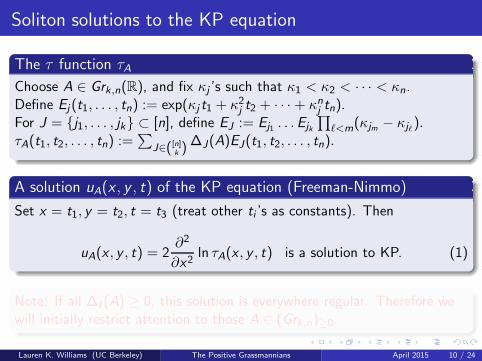
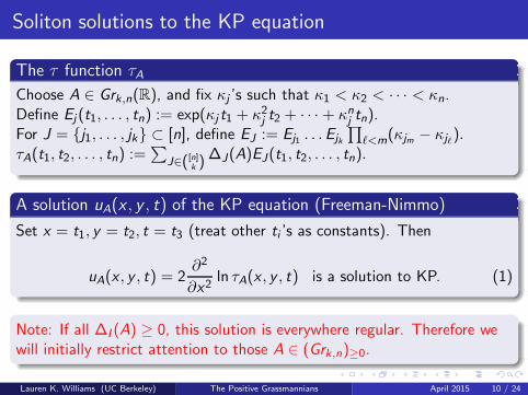
Choose A ∈ Grk,n(R), and fix κj ’s such that κ1 < κ2 < · · · < κn.Define Ej (t1, . . . , tn) := exp(κj t1 + κ2j t2 + · · · + κnj tn).For J = {j1, . . . , jk} ⊂ [n], define EJ := Ej1 . . .Ejk
∏
ℓ<m(κjm − κjℓ).τA(t1, t2, . . . , tn) :=
∑
J∈([n]k )∆J(A)EJ(t1, t2, . . . , tn).
A solution uA(x , y , t) of the KP equation (Freeman-Nimmo)
Set x = t1, y = t2, t = t3 (treat other ti ’s as constants). Then
uA(x , y , t) = 2∂2
∂x2ln τA(x , y , t) is a solution to KP. (1)
Note: If all ∆I (A) ≥ 0, this solution is everywhere regular. Therefore wewill initially restrict attention to those A ∈ (Grk,n)≥0.
Lauren K. Williams (UC Berkeley) The Positive Grassmannians April 2015 10 / 24
Soliton solutions to the KP equation
The τ function τA
Choose A ∈ Grk,n(R), and fix κj ’s such that κ1 < κ2 < · · · < κn.Define Ej (t1, . . . , tn) := exp(κj t1 + κ2j t2 + · · · + κnj tn).For J = {j1, . . . , jk} ⊂ [n], define EJ := Ej1 . . .Ejk
∏
ℓ<m(κjm − κjℓ).τA(t1, t2, . . . , tn) :=
∑
J∈([n]k )∆J(A)EJ(t1, t2, . . . , tn).
A solution uA(x , y , t) of the KP equation (Freeman-Nimmo)
Set x = t1, y = t2, t = t3 (treat other ti ’s as constants). Then
uA(x , y , t) = 2∂2
∂x2ln τA(x , y , t) is a solution to KP. (1)
Note: If all ∆I (A) ≥ 0, this solution is everywhere regular. Therefore wewill initially restrict attention to those A ∈ (Grk,n)≥0.
Lauren K. Williams (UC Berkeley) The Positive Grassmannians April 2015 10 / 24
Visualing soliton solutions to the KP equation
The contour plot of uA(x , y , t)
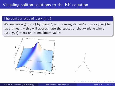
We analyze uA(x , y , t) by fixing t, and drawing its contour plot Ct(uA) forfixed times t – this will approximate the subset of the xy plane whereuA(x , y , t) takes on its maximum values.
Lauren K. Williams (UC Berkeley) The Positive Grassmannians April 2015 11 / 24
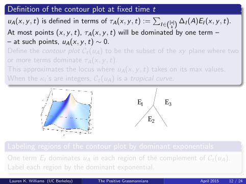
Definition of the contour plot at fixed time t
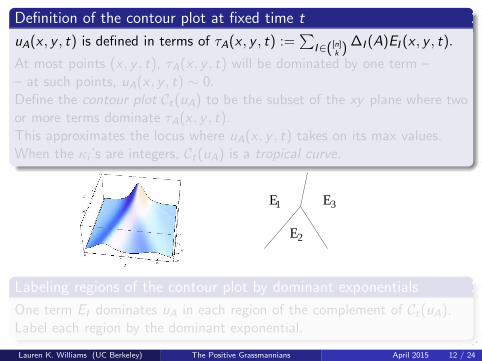
uA(x , y , t) is defined in terms of τA(x , y , t) :=∑
I∈([n]k )∆I (A)EI (x , y , t).
At most points (x , y , t), τA(x , y , t) will be dominated by one term –– at such points, uA(x , y , t) ∼ 0.Define the contour plot Ct(uA) to be the subset of the xy plane where twoor more terms dominate τA(x , y , t).This approximates the locus where uA(x , y , t) takes on its max values.When the κi ’s are integers, Ct(uA) is a tropical curve.
1 3
2
E E
E
Labeling regions of the contour plot by dominant exponentials
One term EI dominates uA in each region of the complement of Ct(uA).Label each region by the dominant exponential.
Lauren K. Williams (UC Berkeley) The Positive Grassmannians April 2015 12 / 24
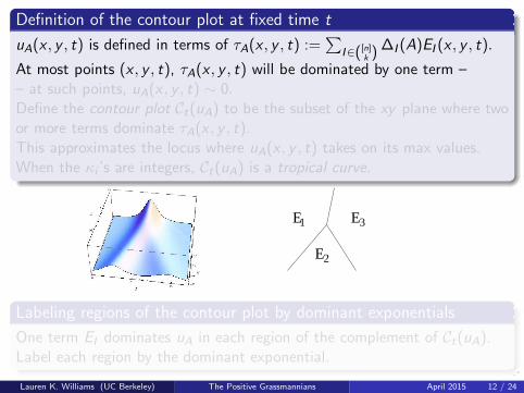
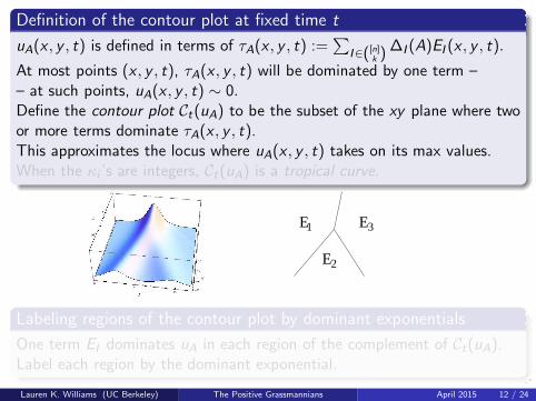
Definition of the contour plot at fixed time t
uA(x , y , t) is defined in terms of τA(x , y , t) :=∑
I∈([n]k )∆I (A)EI (x , y , t).
At most points (x , y , t), τA(x , y , t) will be dominated by one term –– at such points, uA(x , y , t) ∼ 0.Define the contour plot Ct(uA) to be the subset of the xy plane where twoor more terms dominate τA(x , y , t).This approximates the locus where uA(x , y , t) takes on its max values.When the κi ’s are integers, Ct(uA) is a tropical curve.
1 3
2
E E
E
Labeling regions of the contour plot by dominant exponentials
One term EI dominates uA in each region of the complement of Ct(uA).Label each region by the dominant exponential.
Lauren K. Williams (UC Berkeley) The Positive Grassmannians April 2015 12 / 24
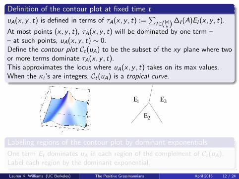
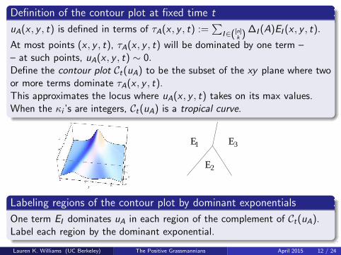
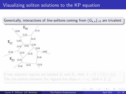
Visualizing soliton solutions to the KP equation
Generically, interactions of line-solitons coming from (Gk,n)>0 are trivalent.
[1,3]
[1,5]
[1,6]
[2,6]
[3,4]
[4,6]
[3,6]
[2,6]
[2,3]
[2,5]
[1,5]
[1,2]
[5,6]
[3,5][4,5][2,4]
[2,5]
[3,5]
23
12
16E
E
E
If two adjacent regions are labeled EI and EJ , then J = (I \ {i}) ∪ {j}.The line-soliton between the regions has slope κi + κj ; label it [i , j].
Lauren K. Williams (UC Berkeley) The Positive Grassmannians April 2015 13 / 24
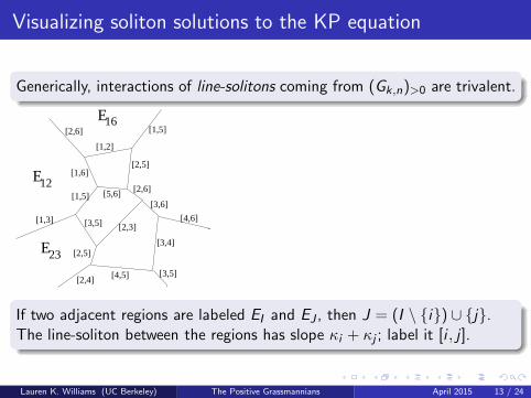
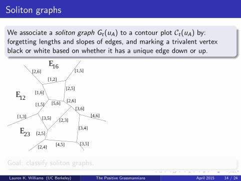
Soliton graphs
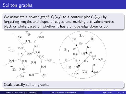
We associate a soliton graph Gt(uA) to a contour plot Ct(uA) by:forgetting lengths and slopes of edges, and marking a trivalent vertexblack or white based on whether it has a unique edge down or up.
[1,3]
[1,5]
[1,6]
[2,6]
[3,4]
[4,6]
[3,6]
[2,6]
[2,3]
[2,5]
[1,5]
[1,2]
[5,6]
[3,5][4,5][2,4]
[2,5]
[3,5]
23
12
16E
E
E
Goal: classify soliton graphs.
Lauren K. Williams (UC Berkeley) The Positive Grassmannians April 2015 14 / 24
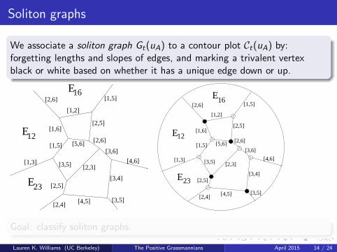
Soliton graphs
We associate a soliton graph Gt(uA) to a contour plot Ct(uA) by:forgetting lengths and slopes of edges, and marking a trivalent vertexblack or white based on whether it has a unique edge down or up.
[1,3]
[1,5]
[1,6]
[2,6]
[3,4]
[4,6]
[3,6]
[2,6]
[2,3]
[2,5]
[1,5]
[1,2]
[5,6]
[3,5][4,5][2,4]
[2,5]
[3,5]
23
12
16E
E
E
[1,3]
[1,5]
[1,6]
[2,6]
[3,4]
[4,6]
[3,6]
[2,6]
[2,3]
[2,5]
[1,5]
[1,2]
[5,6]
[3,5][4,5][2,4]
[2,5]
[3,5]
E
E
E
16
12
23
Goal: classify soliton graphs.
Lauren K. Williams (UC Berkeley) The Positive Grassmannians April 2015 14 / 24
Soliton graph → plabic graph
[1,3]
[1,5]
[1,6]
[2,6]
[3,4]
[4,6]
[3,6]
[2,6]
[2,3]
[2,5]
[1,5]
[1,2]
[5,6]
[3,5][4,5][2,4]
[2,5]
[3,5]
E
E
E
16
12
23
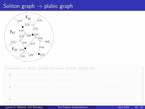
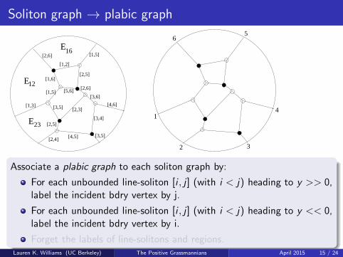
Associate a plabic graph to each soliton graph by:
For each unbounded line-soliton [i , j] (with i < j) heading to y >> 0,label the incident bdry vertex by j.
For each unbounded line-soliton [i , j] (with i < j) heading to y << 0,label the incident bdry vertex by i.
Forget the labels of line-solitons and regions.
Lauren K. Williams (UC Berkeley) The Positive Grassmannians April 2015 15 / 24
Soliton graph → plabic graph
[1,3]
[1,5]
[1,6]
[2,6]
[3,4]
[4,6]
[3,6]
[2,6]
[2,3]
[2,5]
[1,5]
[1,2]
[5,6]
[3,5][4,5][2,4]
[2,5]
[3,5]
E
E
E
16
12
23
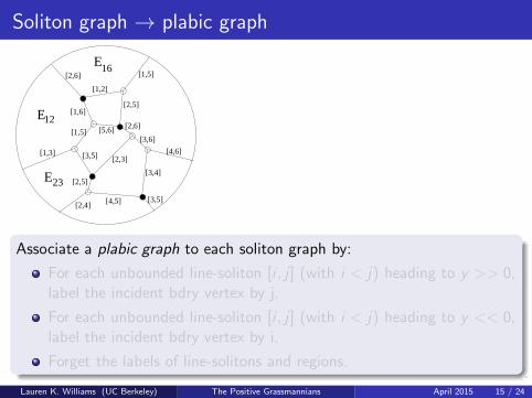
Associate a plabic graph to each soliton graph by:
For each unbounded line-soliton [i , j] (with i < j) heading to y >> 0,label the incident bdry vertex by j.
For each unbounded line-soliton [i , j] (with i < j) heading to y << 0,label the incident bdry vertex by i.
Forget the labels of line-solitons and regions.
Lauren K. Williams (UC Berkeley) The Positive Grassmannians April 2015 15 / 24
Soliton graph → plabic graph
[1,3]
[1,5]
[1,6]
[2,6]
[3,4]
[4,6]
[3,6]
[2,6]
[2,3]
[2,5]
[1,5]
[1,2]
[5,6]
[3,5][4,5][2,4]
[2,5]
[3,5]
E
E
E
16
12
231
2 3
4
56
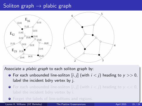
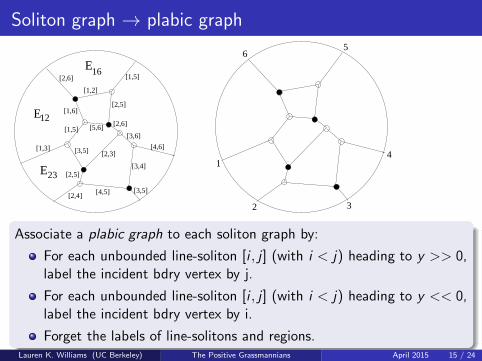
Associate a plabic graph to each soliton graph by:
For each unbounded line-soliton [i , j] (with i < j) heading to y >> 0,label the incident bdry vertex by j.
For each unbounded line-soliton [i , j] (with i < j) heading to y << 0,label the incident bdry vertex by i.
Forget the labels of line-solitons and regions.Lauren K. Williams (UC Berkeley) The Positive Grassmannians April 2015 15 / 24
Soliton graph → plabic graph
[1,3]
[1,5]
[1,6]
[2,6]
[3,4]
[4,6]
[3,6]
[2,6]
[2,3]
[2,5]
[1,5]
[1,2]
[5,6]
[3,5][4,5][2,4]
[2,5]
[3,5]
E
E
E
16
12
231
2 3
4
56
Associate a plabic graph to each soliton graph by:
For each unbounded line-soliton [i , j] (with i < j) heading to y >> 0,label the incident bdry vertex by j.
For each unbounded line-soliton [i , j] (with i < j) heading to y << 0,label the incident bdry vertex by i.
Forget the labels of line-solitons and regions.Lauren K. Williams (UC Berkeley) The Positive Grassmannians April 2015 15 / 24
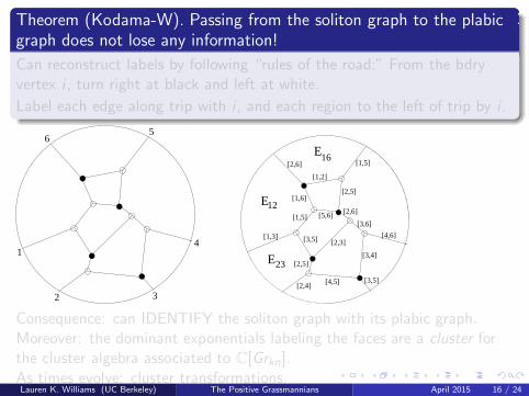
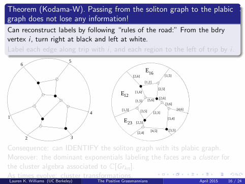
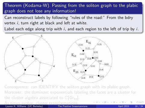
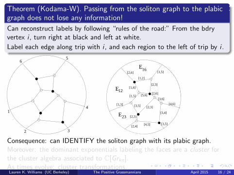
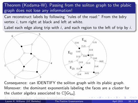
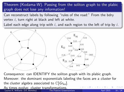
Theorem (Kodama-W). Passing from the soliton graph to the plabicgraph does not lose any information!
Can reconstruct labels by following “rules of the road:” From the bdryvertex i , turn right at black and left at white.
Label each edge along trip with i , and each region to the left of trip by i .
1
2 3
4
56
[1,3]
[1,5]
[1,6]
[2,6]
[3,4]
[4,6]
[3,6]
[2,6]
[2,3]
[2,5]
[1,5]
[1,2]
[5,6]
[3,5][4,5][2,4]
[2,5]
[3,5]
E
E
E
16
12
23
Consequence: can IDENTIFY the soliton graph with its plabic graph.Moreover: the dominant exponentials labeling the faces are a cluster forthe cluster algebra associated to C[Grkn].As times evolve: cluster transformations.Lauren K. Williams (UC Berkeley) The Positive Grassmannians April 2015 16 / 24
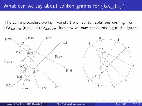
What can we say about soliton graphs for (Grk ,n)≥0?
The same procedure works if we start with soliton solutions coming from(Grk,n)≥0 (not just (Grk,n)>0) but now we may get a crossing in the graph.
[1,3][2,5] [3,7]
[2,4]
[1,5]
[2,5]
[2,3]
[6,8]
[7,9]
[6,9] [4,8]
[8,9]
[6,7]
[4,7]
[4,5]
E1246
E4589
[1,7]
[1,5]
[4,8]
9
8
1
2 3
6
7
5
4
Lauren K. Williams (UC Berkeley) The Positive Grassmannians April 2015 17 / 24
What can we say about soliton graphs for (Grk ,n)≥0?
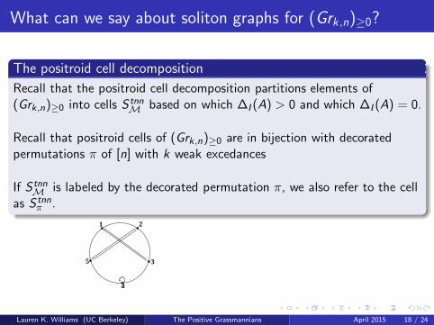
The positroid cell decomposition
Recall that the positroid cell decomposition partitions elements of(Grk,n)≥0 into cells S tnn
M based on which ∆I (A) > 0 and which ∆I (A) = 0.
Recall that positroid cells of (Grk,n)≥0 are in bijection with decoratedpermutations π of [n] with k weak excedances
If S tnnM is labeled by the decorated permutation π, we also refer to the cell
as S tnnπ .
Lauren K. Williams (UC Berkeley) The Positive Grassmannians April 2015 18 / 24
What can we say about soliton graphs for (Grk ,n)≥0?
The positroid cell decomposition
Recall that the positroid cell decomposition partitions elements of(Grk,n)≥0 into cells S tnn
M based on which ∆I (A) > 0 and which ∆I (A) = 0.
Recall that positroid cells of (Grk,n)≥0 are in bijection with decoratedpermutations π of [n] with k weak excedances
If S tnnM is labeled by the decorated permutation π, we also refer to the cell
as S tnnπ .
1 2
3
4
5
Lauren K. Williams (UC Berkeley) The Positive Grassmannians April 2015 18 / 24
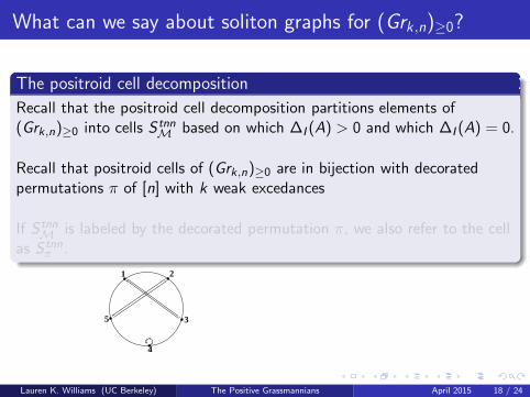
Total positivity on the Grassmannian and KP solitons
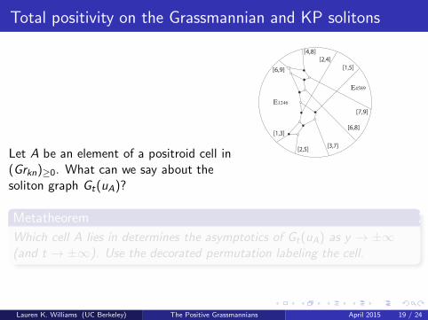
Let A be an element of a positroid cell in(Grkn)≥0. What can we say about thesoliton graph Gt(uA)?
[1,3]
[2,5][3,7]
[2,4]
[1,5]
[6,8]
[7,9]
[6,9]
[4,8]
E1246
E4589
Metatheorem
Which cell A lies in determines the asymptotics of Gt(uA) as y → ±∞(and t → ±∞). Use the decorated permutation labeling the cell.
Lauren K. Williams (UC Berkeley) The Positive Grassmannians April 2015 19 / 24
Total positivity on the Grassmannian and KP solitons
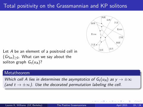
Let A be an element of a positroid cell in(Grkn)≥0. What can we say about thesoliton graph Gt(uA)?
[1,3]
[2,5][3,7]
[2,4]
[1,5]
[6,8]
[7,9]
[6,9]
[4,8]
E1246
E4589
Metatheorem
Which cell A lies in determines the asymptotics of Gt(uA) as y → ±∞(and t → ±∞). Use the decorated permutation labeling the cell.
Lauren K. Williams (UC Berkeley) The Positive Grassmannians April 2015 19 / 24
How the positroid cell determines asymptotics at y → ±∞
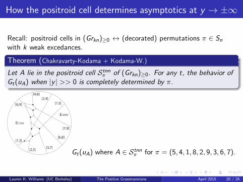
Recall: positroid cells in (Grkn)≥0 ↔ (decorated) permutations π ∈ Snwith k weak excedances.
Theorem (Chakravarty-Kodama + Kodama-W.)
Let A lie in the positroid cell Stnnπ of (Grkn)≥0. For any t, the behavior of
Gt(uA) when |y | >> 0 is completely determined by π.
[1,3]
[2,5][3,7]
[2,4]
[1,5]
[6,8]
[7,9]
[6,9]
[4,8]
E1246
E4589
Gt(uA) where A ∈ Stnnπ for π = (5, 4, 1, 8, 2, 9, 3, 6, 7).
Lauren K. Williams (UC Berkeley) The Positive Grassmannians April 2015 20 / 24
Role of positivity for KP solitons
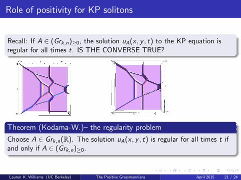
Recall: If A ∈ (Grk,n)≥0, the solution uA(x , y , t) to the KP equation isregular for all times t. IS THE CONVERSE TRUE?
Theorem (Kodama-W.)– the regularity problem
Choose A ∈ Grk,n(R). The solution uA(x , y , t) is regular for all times t ifand only if A ∈ (Grk,n)≥0.
Lauren K. Williams (UC Berkeley) The Positive Grassmannians April 2015 21 / 24
Role of positivity for KP solitons
Recall: If A ∈ (Grk,n)≥0, the solution uA(x , y , t) to the KP equation isregular for all times t. IS THE CONVERSE TRUE?
Theorem (Kodama-W.)– the regularity problem
Choose A ∈ Grk,n(R). The solution uA(x , y , t) is regular for all times t ifand only if A ∈ (Grk,n)≥0.
Lauren K. Williams (UC Berkeley) The Positive Grassmannians April 2015 21 / 24
Thanks for listening!
Scattering amplitudes
Physical process: scattering of n massless particles
External data: momenta and helicities of particles
Role of plabic graphs: allows one to parameterize the positiveGrassmannian. To compute the amplitude, one integrates a form,which is expressed in terms of positive Grassmannian (singularitiesonly on its boundary). Also: one can express the BCFW recurrencevery naturally in terms of plabic graphs.
Soliton solutions of the KP equation
Physical process: Interaction of n solitons (waves which preserveshape) coming from infinity to interact within finite region
External data: Directions (slopes) of the incoming solitons
Integrability: KP hierarchy
Role of plabic graphs: The interaction pattern of solitons AREprecisely tropical realizations of plabic graphs. Cluster charts.
Lauren K. Williams (UC Berkeley) The Positive Grassmannians April 2015 22 / 24
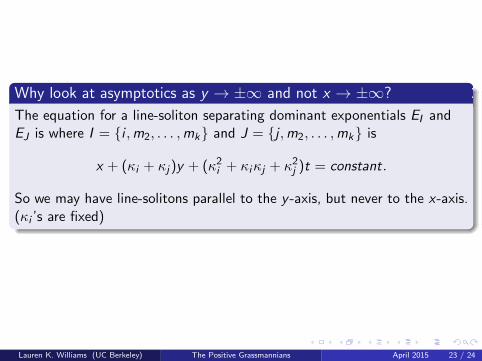
Why look at asymptotics as y → ±∞ and not x → ±∞?
The equation for a line-soliton separating dominant exponentials EI andEJ is where I = {i ,m2, . . . ,mk} and J = {j ,m2, . . . ,mk} is
x + (κi + κj)y + (κ2i + κiκj + κ2j )t = constant.
So we may have line-solitons parallel to the y -axis, but never to the x-axis.(κi ’s are fixed)
Lauren K. Williams (UC Berkeley) The Positive Grassmannians April 2015 23 / 24
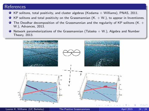
ReferencesKP solitons, total positivity, and cluster algebras (Kodama + Williams), PNAS, 2011.
KP solitons and total positivity on the Grassmannian (K. + W.), to appear in Inventiones.
The Deodhar decomposition of the Grassmannian and the regularity of KP solitons (K. +W.), Advances, 2013.
Network parameterizations of the Grassmannian (Talaska + W.), Algebra and NumberTheory, 2013.
Lauren K. Williams (UC Berkeley) The Positive Grassmannians April 2015 24 / 24


![Towards the amplituhedron volume - uni-muenchen.de2016)014.pdftwistor space [13] and then in momentum super-twistor space [14], Grassmannian integrals compute scattering amplitudes](https://static.documents.pub/doc/80x56/5f0873457e708231d4221281/towards-the-amplituhedron-volume-uni-2016014pdf-twistor-space-13-and-then.jpg)
![City Research Onlineof encoding scattering amplitudes in N= 4 super-Yang-Mills theory in terms of planar bipartite graphs and cells in the positive Grassmannian [17{21]. Amongst these](https://static.documents.pub/doc/80x56/5f0873497e708231d4221295/city-research-online-of-encoding-scattering-amplitudes-in-n-4-super-yang-mills.jpg)
