The Power of Love: A Subtle Driving Force

for Unegalitarian Labour Division?

Luise Goerges∗

Universitaet Hamburg

E-Mail luise.goerges@wiso.uni-hamburg.de

April 23, 2014

Abstract

In this paper, I experimentally investigate couples’ specialization decisions and examine

the gender-specific patterns in labour division arising within heterosexual couples. Eighty

participants—20 real couples and 20 pairs of strangers—play a two-stage game, paired up

either with their partner or a stranger of the opposite sex. In the first stage, participants

make a joint decision on how to play the game: They can both complete a performance-

based paid task (task A) or have one of the players perform an unpaid task (task B), thereby

tripling the pay-rate for their partner playing task A. After completing their tasks, partic-

ipants are informed about their pay-offs in private and then asked to make an individual

decision about what proportion of their income to pay into a common pool, where it is

increased by 20% and distributed equally between the two players. I find that women are

significantly more likely to give up their income autonomy and perform the unpaid task

when playing with their partner rather than with an unfamiliar man. Men’s behaviour is

not affected by familiarity with their female partner.

JEL Codes: B54, C92, D13

Keywords: experiment, spousal labour division, intra-household bargaining, female labour

supply, income inequality

∗Acknowledgements: I conducted the experiment with financial research support provided by the University

of Warwick. I am grateful for advice and helpful comments from Miriam Beblo, Bart Golsteyn, Daniel Hamer-

mesh, Martin Heidenreich, Thomas Hills, Ulf Kadritzke, Peter Kuhn, Andreas Lange, Marcus Nöth, Annemarie

Paul, Arne Pieters, Helmut Rainer, Thomas Siedler, the participants of a workshop on experimental economics

and a seminar on family economics at the Universitaet Hamburg, as well as from two anonymous referees. All

remaining errors are my own.

i

1 Introduction

“Often there are fundamental inequalities in gender relations within the family or the

household. (. . . ) It is quite common in many societies to take for granted that men will

naturally work outside the home, whereas women could do so if and only if they could combine

such work with various inescapable and unequally shared household duties. This is sometimes

called ‘division of labour’, though women could be forgiven for seeing it as an ‘accumulation of

labour’. The reach of this inequality includes not only unequal relations within the family, but

also derivative inequalities in employment and recognition in the outside world.”

?

The motivation for this study arises from a puzzling observation closely connected to Sen’s

statement that, after a decade, does not appear to have lost its validity: In most European

households, couples fail to achieve an equal sharing of paid, labour-market work and unpaid,

household-related work. Instead, despite their improving educational achievements and pro-

fessional qualifications, women are frequently observed to devote their labour primarily to

family-work. Many of them still only become active in the labour market to the extent their

remaining capacities allow them to. This is one of the main reasons why even modern devel-

oped societies have failed to achieve gender equality in the labour market. Many inequalities

persist and hinder female economic independence (??).

In this paper, I present experimental evidence on couples’ decisions on dividing paid and

unpaid labour and compare their behaviour to mixed-sex pairs of strangers. The main questions

addressed here are whether couples divide labour more often in order to reach efficiency gains

when this requires the individual disadvantage of one of the partners, and, if so, whether male

and female partners are equally likely to undertake the disfavoured role in absence of individual

productivity differences.

Most of the specific gender inequalities observable in European labour markets are inter-

dependent with household-related work which is still predominantly provided by women (??).

In 2012, though with remarkable differences between countries, the average rate of female

labour market participation was 62.3% within the EU-27, compared to 74.6% for men. As the

household-related workload increases, especially when entering parenthood, this employment

gap usually widens: figures for adults aged 25 to 49 provided by ? show, when entering par-

enthood, women’s participation in the labour market decreases by about 10 percentage-points

while men’s increases by the same amount. While the share of male inactives or part-time-

employed males in the same age-group, who state "child-rearing" or other family-related duties

as the main reason for not seeking (full-time) employment is well below 10% in the EU-27,

1

among females, this share amounts to about 40% (??). Consequently, women often face addi-

tional career-penalties, such as lower wages, fewer chances for promotion, etc. (?). Thus, as a

result of gender-specific labour division, we observe women to give up their income autonomy

more frequently, thereby becoming dependent on their partners’ income and running a higher

risk of descending into poverty.

Economic theory provides different accounts to explain the gender-specific patterns in

labour division between couples. Both new home economics and economic bargaining ap-

proaches identify structural differences in expected returns to labour market activity for men

and women (in terms of wages, likelihood of promotion, etc.) as a key determinant for the

households’ decision on the concrete form of its labour supply – i.e. who is going to supply

how much labour. From a policy perspective, they yield a similar insight as they suggest the

following: If spouses imposed equivalent opportunity costs on the household by withdrawing

from the labour market in favour of household production, then either spouse will do so with

equal probability1. We would expect to find roughly equivalent opportunity costs when part-

ners have comparable characteristics in terms of their education and experience and if the

demand side for labour does not discriminate systematically against one sex. Over the past

decades, European society has made substantial progress with respect to these preliminaries,

e.g. steady rises in female educational attainment on the supply side and affirmative action

policies on the demand side (?). These improvements should level the opportunity costs that

males and females impose on their common households when they abstain from the labour

market. Yet, within the vast majority of families, we still observe a form of labour division

where the women cut back from labour market participation (??).

These observations inevitably lead one to question the accuracy of an analysis focusing on

gender differences in expected labour-market outcomes as the main reason for unequal labour

division within couples. The answer to this question has important implications for equalizing-

policy: If eliminating gender differences in expected returns to labour market activity (e.g.

by raising female educational attainment, affirmative action, etc.) is not sufficient to ensure

that couples’ decisions on labour division will disadvantage one or the other partner with equal

probability, the structural problem of female “underachievement” in the labour market will

persist. Therefore, current policy approaches to improve female labour-market outcomes may

promise only limited success if men’s and women’s decisions on paid-labour participation differ

depending on the social context they are made in – in this case, an individual versus partnership

context.1Assuming, of course, that a withdrawal of either of them is still beneficial for the overall household welfare

– i.e., purchasing household services externally imposes higher costs than one partner’s (partial) labour marketabsence.

2

The contribution of this paper is to provide a direct, experimental test of this hypothesis.

To the best of my knowledge, none of the few economic experiments concerned with couples’

decision-making conducted so far focus on the participants’ decisions on labour division.2 It

is a unique feature of the experiment presented here that it allows for a careful examination

of how women and men divide paid and unpaid labour if objective measures on their individ-

ual productivity (i.e. expected pay-off), and hence potential gender differences in expected

outcomes, are not available a-priori. Moreover, it allows for examination of how this decision

changes within two particular social contexts: together with a stranger of the opposite sex or

with one’s real-life partner.

To achieve this, I recruited 20 real couples and 20 pairs of strangers and asked them to

play a two-stage game; paired up either with their partner or a stranger of the opposite sex.

In the first stage, participants make a joint decision on how to play the game: They can both

complete a performance-based paid task (task A) or have one of the players perform an unpaid

task (task B), thereby tripling the pay-rate for their partner playing task A. After completing

their tasks, participants are informed about their pay-offs in private and then asked to make an

individual decision about what proportion of their income to pay into a common pool, where

it is increased by 20% and distributed equally between the two players. If couples maximize

a joint utility function, or bargain cooperatively, they should be more likely than strangers to

tolerate income-inequality and realize the efficient outcome (i.e. divide labour and play the

combination A/B as opposed to each playing the paid task A individually). Furthermore, since

neither men nor women know their productivity in either task, they should be equally likely

to perform the unpaid or the paid task when dividing labour, irrespective of whether they

cooperate with a stranger or with their partner. In order to verify that behavioural differences

between familiar and unfamiliar participants can not be attributed to a selection mechanism, I

additionally collect a large number of personality trait and attitude measures that are typically

thought of as driving factors for (gender-specific) differences in labour-market orientation.

The remainder of this paper is organised as follows: Section 2 sketches the theoretical

accounts offered by economic theory to explain the phenomenon of gender-specific labour di-

vision within couples. Section 3 contains a brief overview of the experimental literature that

revolves around gender and family economics. Section 4 describes the methodology used for

the experiments presented here, followed by section 5, which provides a description of the main

results. Section 6 contains a summary of sensitivity analyses in order to verify the robustness

of the findings. The discussion in section 7 offers some potential interpretations of the results.2? investigate the effects of individual vs. joint taxation on couples’ labour supply, modelled as individual

work effort. ? explore how couples distribute resources when the initial allocation is determined exogenouslyvs. endogenously (i.e. resulting from their individual work-effort). ? document the attempt to investigatepartners’ provision of unpaid work vs. enjoying leisure-time experimentally.

3

Section 8 concludes the experiment and discusses implications for further research.

2 Theoretical Background

Economists have developed various theoretical approaches to model the family decision-making

process, which can broadly be divided into three main strands. The first is the unitary house-

hold utility model in the “new home economics” mainly developed by Becker from the 1960s

onward (and conflated in his “Treatise on the Family” 1991). The second and third strand in-

volve models based on economic bargaining theory, namely cooperative (pioneering work came

from ??) and non-cooperative (??, , initially) bargaining models. Here, I will only briefly

describe the three strands and how they relate to the experiment, which allows me to test

some derivative model predictions (for a general overview, see ??).

The unitary household utility model (?) as postulated in the new home economics offers an

explanation for why we often observe a specific pattern in intra-family labour division. Accord-

ing to this model, the characteristic gender gap in paid labour-market and unpaid household-

related work participation derives from wives’ lower expected returns to labour market activities

relative to their husbands’.3 The theory suggests that spouses, since they are assumed to maxi-

mize their joint utility4, base their decision about who will cut back labour-market engagement

in favour of household work – especially after entering parenthood – on the partners’ individual

labour market opportunities: The spouse who can expect a lower pay-off from labour-market

activity imposes lower opportunity costs on the household when giving up labour-market work

in favour of household work.

Following this rationale, the model predicts specialization to occur whenever it yields effi-

ciency gains that allow couples to reach a higher joint utility level. Unequal conditions in the

labour market promote productivity differences between women and men, which is why, within

a resource-pooling household, it is in both partners’ best interests to allocate males’ labour to

the market and females’ to the household. By using their individual comparative advantages,

partners maximize their joint utility. It follows that, in the absence of comparative advantages,

partners should be equally likely to specialize in one or the other production.

Intra-household bargaining approaches that model household decisions, on the other hand,

do acknowledge diverging interests within the household, thus rejecting the idea of a com-

mon utility function. In bargaining theories, household decisions are viewed as resulting from3Strictly speaking, a productivity (dis-)advantage in labour market activities is not a necessary requirement.

Becker himself claims a biologically determined comparative advantage for women in household-related work,particularly in child-rearing (see ?).

4This perspective does not account for potentially diverging interests within the household; it assumes thathousehold members form an entity with a unitary utility function.

4

negotiations between the members. Here, household-related work is assumed to display an

imposition both partners seek to avoid. The partner with the higher bargaining power will be

able to confer most of this inconvenience upon her spouse. Individual bargaining power within

a relationship is often thought of as being determined by a partner’s outside options, e.g.by the

share of household income contributed by each partner. Hence, gender-related differences in

expected labour market outcomes will strongly influence the intra-household-bargaining pro-

cess, especially with respect to labour division and allocation of resources. One main difference

exists between cooperative and non-cooperative bargaining approaches: The former rests on

the assumption that spouses will always reach the efficient outcome (i.e., they will come to an

agreement somehow), whereas the latter does not.

Although unitary household utility approaches and intra-household bargaining approaches

may differ with respect to the question if partners’ agree on specialization, they yield similar

predictions regarding which specific labour division arrangements are most likely to evolve:

Lower expected returns from labour-market activity for females either lead to a comparative

advantage in household production or to a bargaining disadvantage in negotiations concerning

who will be responsible for household work. Either way, when facing labour-market inequalities

to their disadvantage, women are thus more likely to reduce paid market activity in favour of

unpaid household-related work. However, this need not be the case when household decisions

are determined by non-cooperative bargaining and, moreover, should not occur when expected

returns from labour-market activities are equal. The following section seeks to provide a brief

overview of the experimental contributions made so far in an attempt to test which theory

predicts couple behaviour the most accurately.

3 Related Literature

So far we have established that, according to family economic theories, the decision on labour

division between household members follows some kind of expected (joint or individual) utility

maximization. Generally, a wide range of experimental evidence suggests that expected utility

maximization might not be an accurate predictor of people’s choices.5 More specifically, viola-

tions of expected utility theory become particularly likely once an individual’s decision affects

others, and his outcomes are in turn affected by other actors.6 This indeed applies to many, if

not most, real-world decisions, especially within the household context.

Notably, an overwhelming majority of this evidence stems from economic labouratory ex-5For example, very prominently demonstrated by ?.6Illustrative evidence can be found in dictator games, ultimatum games, public good games, (see for example

?????).

5

periments recording outcomes of strategic games played among strangers. Variations on the

degree of information provided about fellow players show, however, how increasing familiarity

with a partner affects outcomes (e.g. ???). Not surprisingly, the tendency to exhibit oppor-

tunistic behaviour seems to decrease while the willingness to cooperate increases with the

tightness of social ties (??).7

Couples’ decisions have been subject to a variety of experimental studies, since they are

often subject to a trade-off between efficiency and equality. The majority of these studies

focus on the standard new home economics approach and aim to reveal its predictions to

be inaccurate. The model’s major shortcoming derives from its failure to acknowledge that

interests and preferences within the household, in reality, may well diverge. Experimentally,

this has been shown by, for example, ????. Their findings suggest that couples may not simply

pool their incomes, nor do they seem to make unitary decisions (let alone have homogeneous

preferences) and maximize aggregate pay-offs—hence, they fail to reach the efficiency outcome

predicted by the theory. Other authors’ experimental findings provide evidence supporting

this notion: Testing spouses’ preferences for equality versus efficiency when choosing a pay-off

distribution, ? and ? find their participants to prefer equality more often. In a recent study,

? compared experimental results for German and French couples who were confronted with an

equity-efficiency problem: Both groups displayed a significant inequality aversion, which was

more pronounced among German couples.

? study the conditions under which specialization arises, an idea which is related more

closely to the research question underlying this paper. However, they examine anonymous

interactions between randomly matched partners in a standard student subject pool. Within

this particularly abstract experimental setting, they challenge the unitary household and bar-

gaining models, arguing that spouses’ specialization in order to realize welfare gains requires

the “household-specializer” to be willing to sacrifice bargaining power (in the form of financial

autonomy) toward her spouse. This introduces asymmetric costs of labour division. Experi-

mentally, they model this within the framework of a semi-structured bargaining game over the

division of a common pot. In the first step, one player gets to choose the size of the pot: Choos-

ing the smaller pot leaves him and his counter player with symmetrical disagreement pay-offs

for the subsequent bargaining stage over the common pot; choosing a larger pot, however,7For example, ? conduct experiments to investigate the behaviour of families in public good games. They

ask participants to decide how much of their private endowment or pay-off they invest into a common pool;the amount collected is then multiplied by some factor greater than one and re-distributed in equal sharesamong all players, regardless of their initial contribution. The authors find that family members contributehigher shares (and hence generate higher overall pay-offs) when playing among themselves only, as opposed toplaying in mixed groups with strangers. ? demonstrate that, in symmetrical prisoner’s dilemma games, 73%of participants cooperate when playing with their partners, as opposed to only 43% of those playing with astranger of the opposite sex.

6

imposes asymmetric disagreement pay-offs on the players, to the disadvantage of the chooser.

Clearly, ? design their bargaining game to mimic real world situations: Specialization

increases overall income, while reducing bargaining power for the partner specializing in house-

hold production (usually the wife), thereby trading off equality against efficiency. However,

in the experimental set-up designed by the authors, participants choose the presumed conse-

quences, not the labour division itself. Thus, they choose the likely outcome of labour division

(i.e., a smaller pot combined with symmetrically distributed bargaining power vs. a larger

pot inducing asymmetric bargaining power). Furthermore, since they play with completely

anonymous partners, “real” gender effects are not subject to the authors’ analysis. Instead,

they focus on analysing a typical “wife decision problem” on a more abstract level.

Partially contradicting the standard game-theory predictions, ? find that “wife players” do

actually choose the variant with the larger pot, at least as long as the asymmetry it imposes on

the individual disagreement pay-offs is not too large. The authors conclude that if the decision

to specialize in household production at a personal cost is additionally framed in an affective

relationship, the actual share of people willing to sacrifice their bargaining power in order to

maximize aggregate welfare might be even higher in reality. However, they do not address the

implications of the gender bias in this particular ‘willingness to sacrifice’ observable in real life

where the majority of “these people” are actual women, not just wife players. The important

insight their study offers concerns the question of whether people bargain cooperatively or

non-cooperatively. The results suggest this to depend on the potential gains of cooperation

relative to the degree of asymmetry in costs it imposes on the partners. Since they find that

even complete strangers with minimal knowledge about their partners will cooperate quite

frequently when this asymmetry is relatively small, we might expect couples to accept even

larger asymmetries in costs before they switch from cooperative to non-cooperative bargaining.

The experiments sketched above mostly present couples (or pseudo-couples) with decision

and bargaining problems that involve the distribution of monetary pay-offs as such and do not

explicitly focus on the decision of how to divide labour. This has, to the best of my knowledge,

not been studied experimentally. Studies analysing gender-specific time disposal (a direct

outcome of labour division within a couple) correspond to the underlying research question of

this paper more closely, but are mostly based on survey data. International European time-use

data shows a gender gap in the average weekly workload for non-single parents in employment

across virtually all EU-27 countries: Women work more (paid and unpaid work combined) and

enjoy less leisure time (see ?, 40). Contrary to the experimental studies on intra-couple income

distribution sketched above, econometric studies exploiting time-use data rather support the

notion of partners realising efficiency gains at the cost of equality. Generally, when couples

7

are found to practice more asymmetric labour division, this is often interpreted as evidence in

favour of the cooperative bargaining model.

Indeed, the gap in time spent on household-related activities appears to be influenced by

the share women contribute to overall household income: For example, ? show a woman’s

relative bargaining power to increase the more she specializes in labour-market production. ?

and ?, using time-use data from Australia and Germany, respectively, show that women are

able to reduce their workload in the household when increasing the share they contribute to the

monetary income of the household, until these contributions are equal. But strikingly, when

women contribute even more, their household-related workload increases again. The authors

interpret this as the point where “gender trump(s) money” (?), or, more precisely, a ‘penalty’

for violating the prevailing social norms. Indeed, this observation might point to some sort of

cognitive bias, as in many developed countries modern couples may hold the ideal of gender

equality as an abstract desirable goal in their minds but have not yet been able to incorporate

it into their daily routines and habits (???). The experiment described in the following section

aims to determine whether this apparent bias can be observed in the lab.

4 Methodology

4.1 Hypotheses

The experiment described here aims to contribute to an important question arising from eco-

nomic theories of the household. Do couples always realize efficiency gains when this requires

specialization in tasks? And are their specialization patterns gender-neutral when comparative

advantages are not related systematically to one sex? I intend to test the following hypotheses:

(1) Couples are more likely than strangers to agree on realizing efficient outcomes (welfare

gains) when this creates inequality (by requiring one player to give up income autonomy).

(2) When playing with their real partner, women are more likely than men to give up income

autonomy in order to reach efficiency gains.

The first hypothesis is uncontroversial from a unitary utility model or a cooperative bargain-

ing model perspective. Previous experimental studies demonstrate how familiarity increases

participants’ willingness to cooperate: For example, family members show a higher contribution

rate in public good games (?) and individuals playing a prisoners’ dilemma with their spouses

choose to cooperate nearly twice as often as those playing with strangers (?). The latter finding

is robust even when pay-offs are asymmetric. Non-cooperative bargaining, however, may lead

8

to a different outcome, especially when partners perceive the asymmetry of individual costs as

high (?), thus resulting in a higher probability of failure to reach the efficient outcome.

The second hypothesis is, however, clearly at odds with the predictions derivable from any

of the theory strands discussed. If cooperation occurs more often among familiar couples, then

male and female partners should, in theory, give up income autonomy (specialize in unpaid

household-related work) with equal probability, assuming there is no comparative advantage

for paid and unpaid tasks that is systematically related to one sex. But if familiar women

are willing to perform an unpaid task more frequently than their unfamiliar counterparts, this

will lead to an unequal distribution of independently controlled income within familiar couples.

Female partners may be right to expect their partners not to exploit their advantage but to

behave reciprocally instead, thus rewarding her for sacrificing her equal position deliberately

(as documented in ?). However, in terms of unconditional access to individual income, they

subsequently depend more on their partner’s good will than unfamiliar females.

In order to test the first hypothesis, the act of performing a paid and an unpaid task must

provide the unity of two players with a larger income than the pairs that perform two paid

tasks individually, thus representing the efficient outcome. In addition, the pay-out rules must

reveal a-priori that realizing the efficient outcome will generate income inequality among the

two players.

To make the second hypothesis testable, the exact nature of the tasks must be unknown to

participants. Consequently, partners should not anticipate gender differences in their expected

pay-offs. More precisely, for the hypothesis to be rejected, women should not be more likely to

undertake the unpaid task, regardless of whether their male partner is a stranger or their real

partner.

4.2 Experimental Design

In two different treatment groups, participants are paired up either with their partner or with

a stranger of the opposite sex. They are asked to make two different decisions, at two different

stages of the game. At the first stage, players must decide jointly if and how they want to

divide labour. They have two real-effort tasks to choose from: Task A, a quiz which offers

a performance-based pay rate for each correct answer and task B, an “assisting” task, that

must be completed complementary to the paid task, but does not in itself yield any pay-off8.

Instead, it triples the pay rate for the task-A performer. They can either:

(i) Work individually (both each spend ten minutes on task A, for individual performance-8Participants had to type their partner’s answers for task A from a paper-pencil answer sheet into a spread-

sheet on a computer. The exact nature of either task is unknown to the participants. They are made aware,that both tasks involve real effort and that their completion is mandatory in order to generate a pay-off.

9

based pay-offs); or

(ii) Work together with their partners (one performs task A for a pay-off while the other one

completes task B to triple their partner’s pay-off; however, only the task-A performer

will receive a payment).

Throughout the decision process in step 1 of the first stage (see Table 1 for a chronological

list of each step in the experiment) participants actually face each other and decide together

whether, and how, to divide the tasks. Hence, partners in the control group do not know each

other but are not anonymous. Only after they have reached a decision, partners are separated

into different rooms, where they complete steps 2-4 in private. Thus, participants perform

their tasks individually and afterward decide privately how much of their personal income, if

any, they want to invest in a common pool. This decision is of course conditional on the player

performing the paid task A in the first stage and earning money.

Table 1: Course of the experiment

Stage 1

Step 1 Decision 1 (jointly): Who does which task?

Step 2 Participants perform their “work”

Step 3 Participants receive their pay-offs in privateStage 2

Step 4 Decision 2 (individually): How much of their received pay-off do they want to invest in a common pool? (investmentsare multiplied by 1.2 and the resulting amount is split 50:50for both participants)

The game and all of its stages were explained in detail before participants made any decision

and a set of test-questions ensured that they understand the consequences of all choices available

to them at any given point9. It is important to note that the exact nature of either task is

unknown to the participants prior to their decision. They are solely informed that task A is

some sort of quiz containing many different types of questions from a wide variety of fields,

with the goal of solving as many questions as possible within ten minutes. Each correctly

answered question yields a pay-off (the total amount of which is tripled if one partner does

task B). Task B, as participants were informed, is some kind of “assisting task”, that does not

require a certain level of performance and is solvable for anyone, but also requires effort and

must be completed in order to triple the partner’s pay-off. This way, a priori gender biases

should not evolve because participants cannot regress on any objective measures to estimate

individual productivity. Hence, they should not be able to predict absolute and/or comparative9See Appendix A for the complete experimental instructions participants received.

10

advantages and divide the tasks accordingly. Therefore, if they divide the tasks, males and

females should be equally likely to perform either task A or B in both the familiar and the

unfamiliar condition.

A gender bias in the choices of tasks could still emerge, however, if the tasks were not

"gender-neutral", i.e. if stereo-typical beliefs about one gender possessing a greater ability in

performing a task exist (irrespective of the true ability distribution). It is therefore important

to reflect on the implications for this study, if participants exhibit a pronounced bias in their a

priori beliefs, e.g., if there was a stereotype that women, on average, are better quiz-takers10. If

this was the case, we might observe women to be significantly more likely to play task A than

half of the time, but this would hold constant regardless whether they play with their partner

or a stranger, and the same would of course be true for men.

Furthermore, limiting prior information about the tasks prevents participants from esti-

mating how many correct answers one could realistically score within the given time-interval.

This ensures that the pay-offs remain private information to the individual generating it11.

Following standard economic game theory the following predictions derive: Via backwards

induction, it becomes evident that rational players, when facing their last decision at step 4,

have no incentive to invest anything into the common pool. This is a dominant strategy because

it maximizes individual income for any given strategy of the other player. This holds, regardless

of how their income was actually determined, i.e., whether the other player played task A or

B. Therefore, at the preceding stage, a rational player would always choose to play task A,

since she can anticipate the consequences of playing task B: This strategy will not yield any

pay-off since a rational counter-player will not invest into the common pool. In short, standard

game theory predicts that participants will never cooperate, neither at stage 1 of the game

when they have to choose how to perform the task, nor at stage 2 when they have to choose

an investment into a common pool. Hence, we should observe all participants playing task A

and nobody investing in the common pool. However, we might observe couples cooperating

if they pool incomes to maximize a unitary utility function or bargain cooperatively. Thus,

observing spouses’ behaviour at the first stage and comparing it to unfamiliar participants’

decisions allows to test the first hypothesis.10Since the quiz was introduced as containing a wide variety of different questions, it can be claimed to be a

rather gender-neutral task, as even subjects concerned with stereo-typical beliefs may have expected questionsthat are “typically easy for men but not for women” and those of the opposite type to be just as likely to occur.

11Whether pay-offs are public or private has been shown to have different effects in varying experimentalsettings with couples: In a field experiment conducted by ? in the Philippines, men were more likely to storepay-offs in their personal accounts when they solely were informed about them in private. However, once anindividual’s pay-off was public information to both spouses, men were more likely than women to commit topooled consumption. In a lab experiment conducted by ?, participants were asked to allocate tokens amongthemselves, with each partner having an individual exchange-rate that was private information. The authorsfound a clear majority of partners revealing their private exchange rate in the bargaining task and hence tryingto realize efficient outcomes instead of using the chance to behave opportunistically.

11

The specific design of the game requires one player to be willing to deviate from this domi-

nant strategy in order to maximize aggregate pay-offs. This involves a high risk, as it requires

the player to give up control over his individual income, hence sacrificing his financial auton-

omy. In fact, players’ willingness to cooperate is tested twice: At stage 1 when participants

decide whether or not to cooperate by dividing the tasks, i.e., play either the combination A/A

or A/B, and again at stage 2, when they must decide how much to invest into the common

pool. Thus, it is possible for players to choose a form of cooperation that does not maximize

aggregate welfare, but still increases it without requiring an a priori disadvantage of one player,

i.e., both play the paid task A and invest their income (partly) into the common pool12. If we

observe couples to frequently choose this strategy, this would provide evidence in support of

non-cooperative bargaining models.

4.3 Additional Measures

4.3.1 Socio-demographic Characteristics

After completing the game, participants fill out a questionnaire (see Appendix B) to pro-

vide basic socio-demographic information, including age, gender, family origin, socio-economic

background, subject of study, duration of and satisfaction with their relationship (on a 10-point-

scale) and relationship-related living arrangements and division of housework. In addition, the

questionnaire contains an item to verify that participants in the unfamiliar condition did not

know each other and that participants in the familiar condition were actual couples13.

4.3.2 Measures for Personality Traits and Individual Attitudes

In addition to standard questions about socio-demographic characteristics, the questionnaire

contains specific statements that gauge participants’ degree of consent, thereby providing mea-

sures for certain personality traits, locus of control (LOC) and core self-evaluation as they

are commonly applied. Furthermore, the questionnaire featured items that are typically used

to elicit participants’ taste for “challenge and affiliation”. Further items address participants’

attitudes on gender roles. All of these measures may be viewed as proxies for labour-market

preferences—in fact, a whole body of literature suggests that the gap in female and male labour

market performances can be linked to differences in preferences (for an overview and critical

examination see ?). Accordingly, evaluating whether these variables are related to certain

specialization patterns is crucial to this study.12It is obvious, however, that a disadvantage may still arise, if players do not invest equal shares or if one

partner performed worse in the quiz and therefore simply has less money at his disposal to invest.13Participants were asked to state their partners’ birthday, which you of course are much less likely to know

by heart if you are not involved in a romantic relationship with that person.

12

4.4 Treatment Groups and Participants

Eighty people participated in the experiment. Participants were mainly recruited among the

University of Warwick student body. The game was played in two different treatment groups,

with individually scheduled sessions for each of the 40 pairs:

• Heterosexual couples

• Pairs of strangers, mixed-sex

Participants were predominantly graduate students (53% Masters; 13% PhD) and under-

graduate students (28%); 8% of participants14 claimed not to be enrolled as a student at the

time of the experiment. Participants were recruited via advertising (posters and flyers) on

campus. Couples in the treatment group and unfamiliar individuals for the control group were

recruited via separate advertisements. The distribution of participants over study levels varied

only slightly between the two treatment groups, with the unfamiliar participants comprising

a larger share of Master students and the familiar group representing a relatively larger share

of PhD students. The share of undergraduate and non-students is equivalent in both groups.

The average age of participants was 25.15

Participants in the familiar group by definition are all involved in a relationship. However,

participants in the control group, although unfamiliar with their experimental partner, are

not necessarily single. In fact, 30% of female and 25% of male participants in the unfamiliar

group reported being in a relationship. These compositional differences between the groups

are addressed in section 6, which provides a detailed analysis of potential selection threats to

the robustness of the results.

5 Results

In the following section, I use the collected experimental data to evaluate the stated hypotheses

by answering the following questions: Are familiar couples more likely to cooperate at the cost

of equality and thereby able to realize greater joint outcomes? Are women more likely than

men to give up their individual, independent income when they play with their partner versus

a stranger? Are the gains in aggregate welfare for familiar couples therefore primarily realized

at the expense of female income autonomy?14May not add up to 100 because of rounding.15The exact statistics: M=25.10, SD=4.49. The fact that the sample consists of 92 % university students who

were largely in their mid-twenties should necessarily be born in mind when deriving conclusions. See section 6for a more thorough discussion.

13

5.1 Hypothesis I: Couples are more likely than strangers to agree on real-

ising efficient outcomes when this creates inequality between them.

Table 2: Proportion of Participants Cooperating by Stage and Familiarity

Familiar Unfamiliar

Stage 1: cooperation (specialization) 100% (n=40) 60% (n=40)

Stage 2: partial cooperation (non-specialing players pooling income) — (n=0) 62.5 % (n=16)

Read: In the familiar group, all couples (100%) cooperate by dividing labour in the first stage. In theunfamiliar group 60% of participants divide labour, i.e. 24 out of 40 participants. In the second stage,out of those people who have not divided labour but instead performed the paid task individually, 62.5%cooperate by investing their stage-1-income (partly) into a common pool.

Table 2 shows the proportion of people cooperating at the different stages. At stage 1, the

number of people who specialise by dividing the tasks and play the game as A/B performers

were 40 in the familiar and 24 in the unfamiliar group. Thus, all familiar participants cooperate,

but “only” 60% of unfamiliar players.16 This difference is statistically significant.17

As discussed above, welfare gains can only be reached by choosing a form of labour division

that requires one player to give up control over his personal income and allows the other player

to determine their final pay-off (recall that the task-A player alone receives a pay-off at the

end of stage 1 and thus is the only one to decide about how much to invest in the common

pool at stage 2, i.e., task-A players determine both their own and their partner’s final pay-off).

Presumably, participants will only be willing to perform the unpaid task B when they expect

their partner to behave reciprocally by investing their pay-off in the common pool, thereby

sharing the fruits of their labour.18

Another form of “partial” cooperation evolved among unfamiliar players and is noteworthy.

As shown in the second row in table 2, of the 16 players who did not cooperate at the first stage,

i.e., where both partners completed task A, 10 invested their entire income into the common

pool19, which can be interpreted as an attempt by the players to cooperate while sustaining

individual control over their personal incomes, yet, within this constraint, trying to maximize16Compared to the standard game-theoretic predictions, this might actually be viewed as a surprisingly high

rate of cooperation among strangers. This can be viewed as a form of a trust game, where even completelyanonymous players have been recorded consistently to cooperate by “trusting” (???). The fact that mostparticipants shared a common identity as students could have driven up the cooperation rate. Furthermore,even though participants were assured that their income and their investment decision would be kept secretfrom their partner, it was obvious that at least to the experimenter, they were known instantly – which mighthave also favoured the high investment rate and the small rate of opportunism in the unfamiliar condition.

17χ2(1)=10, p=.001.18Among co-operators in both groups, however, two task-A-players (roughly 10% of familiar and 17% of

unfamiliar co-operators) did not fulfil their part of the deal to the full extent and exceeded opportunism: i.e.,those “defectors” invested only a share of their stage 1 earnings. Although this type of opportunistic behaviourapproaches the homo-economicus behavioural predictions, none of them let their partners down completely. Theminimum invested was 49% of the amount earned in task A among familiar couples and 60% among unfamiliarcooperators.

1980% of them actually managed to coordinate, i.e. both partners mutually invested all their income.

14

aggregate welfare.20 This can be interpreted as a form of cooperation that favours equality of

partners over the efficiency of their joint outcome.

Based on these figures, the first hypothesis cannot be rejected. Familiar couples seem to

strictly prefer efficiency over equality.

5.2 Hypothesis II: When playing with their real partner, women are more

likely than men to give up income autonomy in order to reach efficiency

gains.

Table 3: Number of People Performing Task A and B byFamiliarity and Gender

Familiar UnfamiliarMale Female Male Female

Paid-task-performers (A) 14 6 13 15

Unpaid-task-performers (B) 6 14 7 5

n = 20 20 20 20

Read: In the unfamiliar group, 13 out of 20 males perform task A.

The first row in Table 3 shows the number of males and females performing the paid task A

(of all participants in their treatment group). In the unfamiliar condition, 15 out of 20 females

completed task A, i.e., 75%. When playing with their partners, females are much less likely

to do so, as only 30% of all familiar women perform the paid task. This difference is highly

significant21 and partly due to the fact that couples choose to specialize more often, i.e., the

familiar condition overall has fewer task-A performers. Males, however, are not more likely

to complete task B when playing with their female partner as opposed to a female stranger.

Hence, they act as task-A performers in both groups about two thirds of the time, tests indicate

no significant difference between the conditions. This implies that couples’ higher likelihood

to divide labour derives from women’s greater willingness to perform the unpaid task when

playing with their partner. We can verify this by looking only at those participants who choose

specialization.

The second row depicts the behavioural pattern of participants cooperating at stage 1,

i.e., they play the combination of task A and B. For familiar participants the distribution is

symmetric, as all of them cooperated at the first stage. Thus, familiar male and female task-

A performers (and task-B performers, respectively) total 20. Among unfamiliar participants,20Another possible explanation, which is rather speculative at this stage of research, involves male ostentation:

in particular, males might feel the desire to impress their female partner by signalling they performed well inthe task rather than potentially being suspected to not have generated much money to invest into the pool inthe first place due to poor performance on the quiz.

21Fisher-exact-test: χ2(1)=8.12, p=.004.

15

there are generally more task-A performers than task-B performers, because not all of them

cooperate with their partners. The number of unfamiliar male task-B performers reveals what

proportion of the 15 unfamiliar female task-A performers where co-operators: Since 7 men

performed task B, by definition, 7 women out of the number who performed task A were their

cooperating partners (and vice versa).

Familiar females perform the unpaid assisting task B in 70% of all cases, whereas when

cooperating with strangers in the unfamiliar condition, less than half (only 42%) of females

perform task B. Economic theory suggests, however, that they will perform either task with

equal probability in the absence of a comparative advantage. That is, once they decide to

cooperate with their partners, females and males should be equally likely to perform the unpaid

task. This should hold regardless of whether they cooperate with a stranger or their partner.

As a test of given proportions reveals, the theoretical predictions match the actual decisions of

unfamiliar cooperators very accurately: the probability does not differ significantly from one

half. When cooperating with their partners, however, familiar females’ probability to perform

the unpaid task B is significantly higher than .5.22

5.3 Implication: Higher (Gendered) Inequality Among Familiar Couples

If couples’ higher co-operation rate is driven by females greater willingness to perform the

unpaid task B, then by definition, they sacrifice their income autonomy more often. In order

to quantify the implications of this finding, one may look at the generated pay-offs conditional

on participants’ specialization and pooling decisions. Recall that by cooperating at stage

1 (playing the A/B combination), participants can triple their pay rate per correct answer.

However, only one of the partners is performing the task and hence collecting the pay-off. By

cooperating at stage 2, the accumulated earnings can be increased by yet another 20% and will

then be split equally between both players. The overall pay-off at the end of stage 2, π2i, for

a player i, therefore depends on her own investment decision (the share si invested), and that

of her partner j, given their individual stage-1 pay-offs (π1):

π2i = π1i − si × π1i + (si × π1i + sj × π1j2

)

This is a standard public-good game. The initial endowment π1i over which a player decides

is endogenous, since it depends on her performance xi conditional on playing task A and on

her pay rate ri, which is determined by whether or not her partner j also performs task A or22The exact test-statistic for familiar females is χ2(1)=3.2, p=.037 against the one-sided alternative that the

probability of performing the unpaid task is greater than 0.5. For unfamiliar females, testing against the sameone-sided alternative delivers χ2(1)=.077, p=.609. Thus, their probability of performing task B does not differfrom 0.5.

16

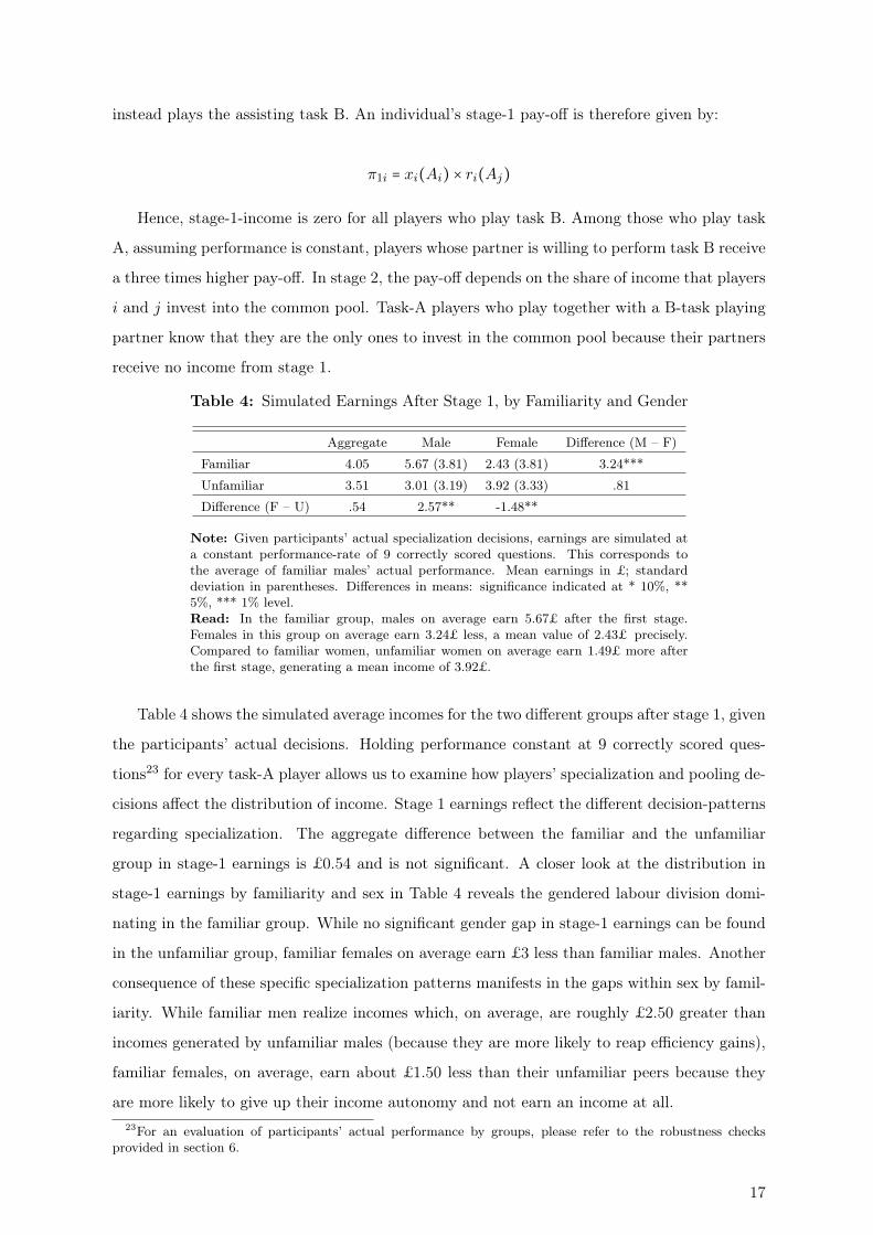
instead plays the assisting task B. An individual’s stage-1 pay-off is therefore given by:

π1i = xi(Ai) × ri(Aj)

Hence, stage-1-income is zero for all players who play task B. Among those who play task

A, assuming performance is constant, players whose partner is willing to perform task B receive

a three times higher pay-off. In stage 2, the pay-off depends on the share of income that players

i and j invest into the common pool. Task-A players who play together with a B-task playing

partner know that they are the only ones to invest in the common pool because their partners

receive no income from stage 1.

Table 4: Simulated Earnings After Stage 1, by Familiarity and Gender

Aggregate Male Female Difference (M – F)

Familiar 4.05 5.67 (3.81) 2.43 (3.81) 3.24***

Unfamiliar 3.51 3.01 (3.19) 3.92 (3.33) .81

Difference (F – U) .54 2.57** -1.48**

Note: Given participants’ actual specialization decisions, earnings are simulated ata constant performance-rate of 9 correctly scored questions. This corresponds tothe average of familiar males’ actual performance. Mean earnings in £; standarddeviation in parentheses. Differences in means: significance indicated at * 10%, **5%, *** 1% level.Read: In the familiar group, males on average earn 5.67£ after the first stage.Females in this group on average earn 3.24£ less, a mean value of 2.43£ precisely.Compared to familiar women, unfamiliar women on average earn 1.49£ more afterthe first stage, generating a mean income of 3.92£.

Table 4 shows the simulated average incomes for the two different groups after stage 1, given

the participants’ actual decisions. Holding performance constant at 9 correctly scored ques-

tions23 for every task-A player allows us to examine how players’ specialization and pooling de-

cisions affect the distribution of income. Stage 1 earnings reflect the different decision-patterns

regarding specialization. The aggregate difference between the familiar and the unfamiliar

group in stage-1 earnings is £0.54 and is not significant. A closer look at the distribution in

stage-1 earnings by familiarity and sex in Table 4 reveals the gendered labour division domi-

nating in the familiar group. While no significant gender gap in stage-1 earnings can be found

in the unfamiliar group, familiar females on average earn £3 less than familiar males. Another

consequence of these specific specialization patterns manifests in the gaps within sex by famil-

iarity. While familiar men realize incomes which, on average, are roughly £2.50 greater than

incomes generated by unfamiliar males (because they are more likely to reap efficiency gains),

familiar females, on average, earn about £1.50 less than their unfamiliar peers because they

are more likely to give up their income autonomy and not earn an income at all.23For an evaluation of participants’ actual performance by groups, please refer to the robustness checks

provided in section 6.

17

Table 5: Simulated Earnings After Stage 2, by Familiarity and Gender

Aggregate Male Female Difference (M – F)

Familiar 4.82 4.21 (.52) 3.89 (.52) .32**

Unfamiliar 3.99 3.10 (1.09) 3.79 (.90) -.69*

Difference (F – U) .83*** 1.11*** .10

Note: Based on the simulated earnings for stage 1, stage-2 earnings are simulatedgiven participants’ actual investment decisions. Mean earnings in £, standard devi-ation in parentheses. Differences in means: significance indicated at * 10%, ** 5%,*** 1% level.Read: In the familiar group, males on average receive £4.21 after the second stage.Unfamiliar males earn a mean value of £3.10

Table 5 shows that the gender differences vanish after task-A performers reward their

task-B-performing partners at the second stage: By investing their income in the common

pool, A-players increase it by 20% and share it equally with their partners. Since nearly all

cooperators24 invest their complete income, at the end of stage 2, reciprocity has smoothed

out the variance in income established at stage 1 and differences in earnings between men and

women within the familiar and unfamiliar group become negligible. As a result, familiarity

remains the only factor to explain the variance in earnings, since it corresponds with a higher

cooperation rate in the first place and since co-operators are more likely to invest their full

earnings into the common pool (where they are again increased by 20%) than non-co-operators.

From Table 5, it also becomes evident that the aggregate difference between familiar and

unfamiliar participants’ final earnings are driven by men. Male participants enjoy significantly

higher terminal earnings when playing with their female partner as opposed to men who play

with a stranger (£1.11, a mark-up of roughly 35%). Thus, they are able to reap the benefits

from specialization. For female participants, surprisingly, playing with their partner does not

yield an advantage over playing with a stranger in terms of the final pay-off generated.

6 Robustness Checks

The validity of the results presented relies crucially on the assumption that participants in

both groups, apart from the differential treatment they receive (playing with their partner

or playing with a stranger), do not differ with respect to other characteristics that might

influence their decisions. This is basically identical to claiming that familiar females would

behave just as unfamiliar females if they played with a stranger. Therefore, the main concern

is whether those females playing with their partner differ systematically in some important

characteristic(s) that in turn make them inclined to choose the assisting task more often. If24As noted earlier, there were two exceptions both among familiar and unfamiliar co-operators, where a task-A

performer was assisted by his partner (i.e., a task-B performer) and did not invest the entire sum earned.

18

this were the case, the results would likely suffer from selection bias. This section offers a closer

examination of potentially confounding variables, in order to mitigate apprehensions in this

regard.

6.1 Performance

Since the findings of this experiment record differential decisions on specialization for familiar

and unfamiliar participants despite the lack of objective measures to predict comparative advan-

tages, the first concern relates to actual productivity: The average number of quiz questions

solved should not differ for men and women within or between both groups.

Table 6: Performance by Familiarity and Gender

Aggregate Male Female Difference |M – F|

Unfamiliar 6.11 (3.23) 6.23 (3.11) 6.00 (3.44) .23

Familiar 8.06 (5.01) 9.09 (4.93) 6.17 ( 5.00) 2.92

Difference |U – F| 1.95 2.86 .17

Note: Mean correct questions given by task-A performers; standard deviation inparentheses. All differences in means are tested with a Mann-Whitney test – none ofthe differences show statistical significance below the 10% level.Read: In the unfamiliar group, participants on average scored 6.11 correct questions,with familiar males scoring a mean of 6.23 and familiar females 6.00.

Table 6 summarizes the average number of correct answers participants gave when per-

forming task A, which overall range from 0 to 16.25 The most important observation is that

differences in participants’ performance do not differ significantly for any group or sub-group

comparison. Despite the lack of significance, by examining the table at face value, one may

still be worried by familiar males’ relatively high performance. My impression throughout

the experiment was that participants who played with their partner were more relaxed and

experienced less anxiety when performing the task.26 Another explanation might be that par-25The results of four participants had to be excluded for calculating the means. They admitted (and their

answer sheets also proved this) to have “cheated”, all of them in the same way: They knew it was impossible tosolve all questions within the given time interval of ten minutes (this was public information), so they reservedthe last minute of their “work time” to randomly guess the multiple-choice answers to those questions they hadnot yet answered. This was not explicitly prohibited, so strictly speaking they were not cheating. However,by doing so they were able to solve presumably roughly as many questions as other participants plus the extrashare scored correctly by chance (wrong answers did not affect income; this was public information, too). Iam able to identify the participants in question (because, during the debriefing, they admitted to have appliedthis strategy) and I can also be sure that this was not the case for any other participant (as their answer sheetwould have revealed such a strategy even if they had not told me). However, I cannot identify exactly how manyquestions “cheaters” were able to “honestly” solve and how many they simply guessed correctly. Therefore, Iam unable to correct their score, which is why I decided to exclude them completely from the analysis of theparticipants’ performance. Three of these cases (all male task-A players) occurred in the familiar group, andone (a male task-B player who “added” guessed answers to his partner’s multiple-choice-answers when copyingthem into the spreadsheet) in the unfamiliar group.

26I have conducted further tests: Recalling the descriptive statistics provided on participants in 4.4 onecould suspect that the higher share of PhD students in the familiar group might pose a problem in terms ofproductivity differences. However, testing the mean scores of PhD students against other participants’ alsoconfirms no significant differences in average performance.

19

ticipants who play the role of “provider” and have to earn income for two people increase their

effort. And indeed, when testing the cooperators’ performance (across both groups) against

non-cooperators’, I find a significant difference: Cooperators on average score 2.36 more an-

swers correctly.27 This is consistent with other experimental studies demonstrating a positive

effect of higher piece-rates on performance (for an overview see ?).

6.2 Trust Level

Perhaps not surprisingly, I find familiar and unfamiliar participants to differ substantially in

their average reported trust level: Paired up with their partners, players report significantly

higher trust (M=9.12; SE=2.27) than unfamiliar partners (M=5.89; SE=2.65)28, on a scale

of 0-10, where 0 represents not trusting one’s partner at all. However, no effect of gender on

the trust levels can be observed, and, more specifically, no interaction between gender and

familiarity—i.e., the increase in trust when playing with one’s partner as opposed to playing

with a stranger does not differ for females and males—which rules out trust as a potential

explanatory variable that could account for the difference in familiar and unfamiliar females’

behaviour. However, it is possible that an increase in trust toward one’s partner, even if it is

quantitatively the same, influences women’s behaviour in different ways than men’s.

6.3 Differences in Attitude and Personality Trait Measures

Among the various personality and attitude measures collected, very few significant differences

were found, neither between sexes nor between unfamiliar and familiar participants. Table 7

summarizes the measures and focuses attention on the same-sex comparison of familiar and

unfamiliar participants, in order to examine whether familiar females display a selection: One

can easily see that the means do not differ significantly for familiar and unfamiliar females in

any of the tested characteristics.29

This is important to highlight for two reasons: (1) The lack of significance in personality and

attitude measures is very relevant in supporting the claim that females in the treatment group

who played with their partners do not form a special selection. (2) Personality trait measures

have recently gained in popularity for explaining (gender) differences in labour-market outcomes

(see for example ???). The fact that they do not seem to govern participants’ decisions on

labour division in this experiment also emphasizes that they should be treated with a reasonable

degree of caution. Some studies partially ascribe the gender gap in labour-market performance27W=1666.5, p=.05. Moreover, it is important to note that, among cooperating task-A players, performance

does not differ significantly by gender.28W=1183.97; p<.00129Again, I have conducted further tests to confirm that there is no significant interaction effect between gender

and familiarity that could explain the difference in the behaviour between unfamiliar and familiar women.

20

to a self-selection driven by differences in personality traits, but they might very well display

a result of gendered labour division instead (compare also the critical examination of reversed

causality between labour-market outcomes and locus of control by ?). At least in the study

described here, participants did not exhibit any significant differences in the personality trait

measures that are often assumed to determine preferences for form and intensity of labour-

market activity (such as locus of control, need for challenge or affiliation, traditional gender

role attitudes). I will therefore briefly describe what these measures intend to capture.

Table 7: Attitude and Personality Trait Measures

Trait or Attitude Measure Gender Familiar Unfamiliar F–U

Traditional gender role attitudeMale 1.6 (.68) 1.4 (.6) .2Female 1.3 (.47) 1.45 (.76) -.15

Locus of control (ext.)Male 12.75 (1.52) 12.15 (2.39) .6Female 13.2 (2.21) 12.9 (2.53) .3

Locus of control (int.)Male 10.85 (1.87) 10.9 (2.14) -.05Female 11.3 (1.66) 10.5 (3.09) .8

ChallengeMale 6.68 (1.16) 6.2 (1.32) .48Female 7.1 (.72) 6.8 (.95) -.3

AffiliationMale 6.95 (1.77) 7.05 (1.0) -.25Female 7.45 (.89) 7.25 (.91) .2

BIG 5

Confidence in successMale 3.35 (.67) 2.95 (.51) -.4**Female 3.3 (.66) 3.32 (.47) -.02

Feeling depressed sometimesMale 1.8 (.70) 2.45 (.94) -.65**Female 2.65 (.88) 2.6 (1.39) .05

Feeling worthless when failingMale 1.95 (.60) 2.45 (.89) -.5**Female 2.2 (1.51) 2.32 (.89) -.15

Doubts about own competenceMale 2.00 (.86) 2.35 (.88) -.35

Female 2.2 (1.01) 2.47 (.7) -.27Determining events in own life

Male 3.35 (.59) 3.25 (.79) .1Female 3.1 (.97) 2.75 (.97) .35

Note: Group means for 4-point scale answers (standard deviation in parentheses), where a highernumber indicates a greater tendency to agree with or (in case of challenge and affiliation) to ratea given item as important. Locus of control and challenge and affiliation are indices containingseveral items, see 6.3.2 and 6.3.3 for details. All differences in means are tested with a Mann-Whitney test. Significance indicated at * 10%, ** 5% and *** 1%- level.Read: Familiar males’ mean answer to the statement “It is a man’s duty to earn the money, whilethe woman takes care of household and family.” is 1.6, which means that, on average, they statedto “disagree” with the statement slightly but insignificantly less often than unfamiliar males (1.4mean).

21

6.3.1 Gender Role Attitudes

Participants were asked to indicate their agreement to the statement "It is a man’s duty to earn

money while the woman takes care of household and family" on a four-point scale (strongly

disagree – strongly agree). If women in the treatment group represented a selection of females

who prefer traditional gender arrangements, we would expect them to agree more often with

this statement. However, this is not the case. One might then hypothesize that this mechanism

could work indirectly through their male partners who might, if they have more traditional

attitudes towards gender-roles, subtly pressure their female partners into playing the assisting

task B. However, the same comparison for males reveals, that they do not differ significantly

in their average agreement with the statement either .

6.3.2 Locus of Control

Locus of control (LOC) is a psychological measure that intends to capture how much a person

believes they are able to actively influence the course of and the events in her life. More

precisely, the construct comprises two measures: The external LOC is an index of items30 that

gauges whether a person considers his life to be governed externally, i.e., a high external LOC

ostensibly means that a person judges his own ability to exert influence in his life to be very

limited. The internal LOC is an index constructed, correspondingly, from items31 intended to

capture the opposite view, i.e., a person considers her life is governed internally. Thus, a high

internal LOC supposedly coincides with the perception that life courses and events are mainly

determined through one’s own actions and decisions. Following these definitions, one might

hypothesize that females who select themselves into a relationship are more likely to exert a

higher external LOC, or a lower internal LOC, respectively,32 and therefore are more likely to

avoid responsibility (e.g., providing for themselves and their partners by performing task A) and

instead try to delegate it to their partners. However, I again fail to detect significant differences

between men and women, familiar and unfamiliar partners, or between the subgroups. This

holds true not only for testing the indices (as presented in table 7) but also when testing each

indivual item within the index.30In particular, it equals the sum of scores assigned to five different statements (items (k)-(o) in the ques-

tionnaire, see appendix B).31The index sums up the scores for items (g)-(j) in the questionnaire.32Precisely this constellation, a high external and a low internal LOC, is often hypothesised to be responsible

for lower labour market outcomes of women, for an overview see ? I will get back to this point in the discussionprovided in section 7

22

6.3.3 Challenge and Affiliation

Two measures that are often linked to labour market success are “challenge” and “affiliation”

indices. In general, people who score high on the challenge items are thought to have a

higher drive for achievement and are hence more career-oriented (i.e., they find it important

or very important to “accomplish something worthwhile” and to have “the chance at getting a

promotion or a better job”33). People who score high on the affiliation items are assumed to

be more agreeable and have a higher need for affiliation (they tend to rate “the friendliness of

the people one works with” and “the respect of other people” important or very important34).

Again, one could speculate whether familiar and unfamiliar females differ with respect to these

characteristics, such that familiar females are less challenge-seeking than unfamiliar females

relative to their partners and/or more affiliation-seeking and therefore prefer to “assist” their

male partners more often rather than “perform” themselves. Again, surprisingly, no significant

differences among the groups can be detected in the sample.

6.3.4 Big Five & Self-confidence

The “standard” personality measures that aim to quantify the degree to which a person exhibits

certain character traits are the so-called “big five”. A number of behavioural researchers ascribe

substantial explanatory power to predicting a wide variety of outcomes to these measures, such

as happiness, health, and especially labour market outcomes (for an overview see for example

??). However, as in the case of locus of control, most studies have not been able to address

reversed causality issues adequately (?). Apprehensions of familiar females displaying a certain

selection—e.g. because women in a relationship may display systematically lower levels of

self-confidence and thus be more likely than unfamiliar females to estimate their own ability,

i.e. productivity, as inferior to their partner—are not supported by the data. In particular,

the items addressing participants’ self-confidence, i.e., the statements "I am confident I get

the success I deserve in life", "Sometimes when I fail I feel worthless", and "I am filled with

doubts about my competence", warrant closer examination. Yet again, there are no significant

differences between the female groups (and also not in comparison to their male partners, not

shown). There are some small differences between familiar and unfamiliar males: familiar males

are, on average, less likely to feel depressed and to feel worthless when failing; and they are

more likely to be confident to get the success they deserve in life . This might be a potential

mechanism that calls for further research. However, these results certainly do not support the

hypothesis that familiar females display a particularly under-confident selection and hence shy33Items (p) and (q) on the questionnaire, see appendix B.34Items (r) and (s).

23

away from the paid task.

6.4 Selectivity of the Student Sample

Further concerns might derive from the selectivity of student subjects who may be viewed as

not representative of the “true” couple population. In addition to the standard reserves toward

student samples used in economic experiments (for a thorough discussion, see ?), I believe

that, due to the increasing popularity of experimental economics and the attention the field

is receiving, another potential source for biases may evolve: A growing subgroup of students

systematically uses experiment participation as an additional income source. Some of them

have become “professional participants”, usually with a certain awareness for the subject of

behavioural and experimental economics. Just as gender can be constructed in the lab (?), the

labouratory homo-economicus might be constructed in a similar way: When participants believe

they are expected to behave according to economic textbook predictions, they might strive for

conformity with such a “homo-economicus-stereotype” in making their decisions within the

experimental context. As a result, students might be more likely to adjust their behaviour

according to standard economic predictions,35 thereby tainting the results from the lab.

In the special case of the experiment presented here, the general dependency on student

subjects combined with students’ relatively high familiarity with the subject in particular,

may arguably strengthen the results. First, more than half of all participants claim to have

taken at least one module in economics. This might have actually helped disguising the actual

research question, as they knew that trust games and dictator games usually aim to examine

participants’ willingness cooperate or defect. However, as most participants confirmed during

the debriefing, they did not expect the underlying research question to be concerned with gender

differences and couples. Second, the dependence on student participants is often considered

problematic because the population the sample is drawn from does not necessarily coincide

with the true population and its social structure; in this case it disproportionately represents

very young and highly educated individuals. In case of the research question underlying this

study, however, this particular over-representation, again, might actually strengthen the results:

While I examine the behaviour of a selection with a presumably very high career- and labour-

market orientation, I still find gender-specific labour division.

Besides age and education level, the couples in the sample are also certainly not represen-

tative of the whole population of couples in terms of relationship duration. Almost half of all

familiar couples were not (yet) cohabitating, and many had not even been together for a year.36

35Or deliberately do the opposite if they construct their identity as explicitly non-conform with standardeconomics predictions. Either way, the effect might be that the observed behaviour deviates from how theywould behave had they not this awareness.

36Precisely, half of all familiar couples reported a time-span of 19 months or less when asked for the duration

24

It thus seems fair to assume that most of the participating couples had not yet established a

sound partnership (in the sense that most of them did not live in a common household). This

supports the notion that, if anything, the gender effect I find might be biased downward, since

for these couples, behaviour might actually be driven by relationship-specific gender stereo-

types in habits and routines to a lesser extent than in the “true” underlying population of all

heterosexual, employable European couples.

7 Discussion

The observed difference in female behaviour when playing with a stranger as opposed to playing

with their real partners does not seem to be driven by differences in individual personality and

attitude characteristics. Thus, it seems unlikely that the results are driven by a self-selection

problem in the samples. Even the level of trust, which increases substantially when comparing

familiar and unfamiliar partners, does not show any variation by sex within the familiar group.

Of course, it is possible that trust affects male and female behaviour differently, but further

research is needed to verify this. Qualitative, structured follow-up interviews could provide a

fruitful way to explore participants’ motives and the driving factors for their behaviour.

Although an analysis that merely relies on non-parametric tests of group means is neces-

sarily limited, the fact that women in the familiar and unfamiliar group do not differ in means

with respect to personality trait measures, is important to highlight. Familiar women are more

likely to play the unpaid task than their male partners even though the design of the two

tasks and their presentation did not provide them with objective measures to infer compara-

tive advantages. At the very least, as the comparisons of personality and attitude measures to

unfamiliar females show, they should not have more reason to assume productivity differences

relative to their male partners.

If men and women in the familiar condition do not differ in their characteristics, neither

with respect to personality traits, labour-market orientation, nor gender role attitudes, how can

the difference in their behaviour be explained? One possible explanation is gender priming.

Studies demonstrate how participants identify with gender-stereotypes when they are cued

(even subtly) and “adjust” their behaviour, often subconsciously, accordingly. The evidence

is rich. For example, ? find that women, who were asked to indicate their gender before

they rate their verbal and mathematical abilities, appraise their verbal skills better and their

mathematical skills worse than members of the control group that were asked to indicate their

ethnicity. Using economic incentives, ? show that whether a specific task activates a positive

or a negative stereotype threat alters women’s (and men’s) willingness to compete significantly:

of their relationship.

25

When the task is perceived as “female”, women are more prone to enter competition. ? also

shows that gender priming can affect both willingness to compete and performance. These

findings illustrate how participants, when confronted with a stereotype, also show a greater

tendency to exhibit behaviour consistent with that stereotype. Applying these insights to this

study, the question becomes: Were familiar players more likely to be affected by “priming” than

unfamiliar players?

Indeed, by construction of this experiment, a priming effect might have been at work:

Participants who were recruited for the control group did not know in advance that the research

question was in any way related to gender or couples. Many of them, as it turned out during the

debriefing, just assumed it was a “standard” behavioural economics experiment designed to test

whether they cooperate or defect. Many openly admitted that they had not even considered the

possibility that I was looking into how they cooperate. Eventually, many of them did not even

pay much attention to the fact that they were playing with a partner of the opposite sex. For

familiar couples, on the other hand, it was inevitably revealed that their relevant characteristic

qualifying them as study participants was their relationship with each other. Even though this

background may not have made them consciously aware of a gender-related research question

(many of them also believed it was attempting to analyse their cooperation and opportunism

strategies), it might still have imposed a much stronger cue to activate their identity as “man”

or “woman”. This may have caused a tendency to behave according to the stereotype in an

effort (whether conscious or unconscious) to comply with social norms.

From an economics perspective one might argue that non-conformist behaviour when facing

a stereotype is costly for the individual and hence it might be perceived as optimal to behave

in line with the stereotype, as long as the costs (in this case: financial independence within

the experiment) do not exceed the costs for acting against the stereotype (here: a woman

taking on the “provider role” within the experiment). ? have attempted to model such costs as

“identity-utility”-loss. The studies of ? and ? cited earlier provide empirical support for this

notion: the desire to comply with gender-specific social norms in heterosexual households may

indeed have measurable effects on how males and females divide household work. Women who

violate the ruling social norms by contributing a larger share to the household’s income than

their male partner must “pay” a penalty for their violation by also (re-) increasing their share

in housework.

Other examples supporting the notion of costs for non-stereo-typical behaviour or deviating

from ruling social norms can be found in the literature on divorce. For example, ? provide

further insights on why and how conformity with social norms might be beneficial for partners:

With a longitudinal survey dataset from the U.S., they show that for women, changes from

26

a traditional gender role attitude to a more progressive one coincide with a decline in their

marital satisfaction level, whereas for men, the effect works in the opposite direction. ?’s (?)

findings establish a link between the family model favoured by a country’s policy at the macro-

level, the practiced gender equality in formal and informal labour division at the micro-level,

and divorce rates. Comparing a country where policy favours the male bread-winner model

(Germany) to a country where national policy does not actively promote a specific family model

(U.S.) allows her to draw the following conclusions: Couples deviating from the politically and

institutionally supported family model in Germany (i.e., practice more gender equality) run a

higher risk of divorce. On the contrary, in the U.S., relationships were more stable when labour

division between spouses took on a more egalitarian form.

Interpreting these results relative to the findings in this experiment offers two (possibly

complementary) explanations: Women in the familiar condition might (subconsciously) ex-

pect some form of ‘penalty’ for behaviour perceived as non-conforming with social norms and

stereotypes. For example, in line with the argument put forward by ?, one such penalty for

non-compliance might arise via a threat on females’ individual level of satisfaction with their

relationship. Following ?, the perceived threat when not behaving according to the prevailing

social norms might (alternatively, or even additionally) stem from an increased risk for the

relationship’s failure.

The possibility that gender differences might be constructed in the labouratory (?) may

also be extended to the real world: If members of a familiar couple are more aware of their

gender identity and therefore form their decisions under this influence, this is presumably true

as well for decisions outside the lab. If gender stereotypes are inescapable in every-day life and

influence decision outcomes by providing benchmarks for socially acceptable behaviour, then

in the lab, as ? put it, they might actually “provide a useful proxy for the real world”.

Examining perceived threats to the relationship or satisfaction within the relationship could

ostensibly help assess men’s and women’s motives when dividing the tasks. These motives,

however, can hardly be elicited by a standardized, anonymous questionnaire alone, which once

more highlights the potential benefits of incorporating qualitative methods into the experiment.

If social norms drive the differences in behaviour, then in the current design, it is almost

impossible to capture these experimentally. Therefore, further investigation of this topic in the

lab should integrate structured; qualitative follow-up interviews.

27

8 Conclusion

In this paper, I presented experimental findings on specialization decisions and labour division

between partners (20 heterosexual couples and 20 pairs of strangers) who played a two-stage

game. Paired up either with their real partner or a stranger of the opposite sex, participants

were asked to make a joint decision on how to play the game in the first stage: They had to

choose whether (1) both would complete a performance-based paid task (task A); or (2) one

of them would perform an unpaid assisting task (task B), thereby tripling the pay-rate for the

task-A player. In the second stage, after completing their tasks, each participant was informed

about her payment in private and asked to make an individual decision on investing his income

(partly) in a common pool, where it was increased by 20% and then split equally between the

two players.

The main results, in short: (1) All familiar couples cooperate, i.e. they play the game in the

A/B combination. In the control group, a considerable share (60%) of unfamiliar participants

cooperate in the same manner, while the rest chooses to play the combination A/A. For familiar

couples, their greater willingness to cooperate at both stages rewards them with higher overall

pay-offs.

(2) When playing with their partner, women are significantly more likely to give up their

income autonomy and perform task B as opposed to the control group with unfamiliar partners,

where the majority chooses to perform task A. For men, no such differences are observed, which

suggest that their behaviour is not affected by familiarity with their female partner. This is

confirmed by comparing only cooperators in both groups: Familiar females’ probability of

performing the unpaid task is significantly larger than 0.5, whereas among unfamiliar female

cooperators, no such deviance can be observed. Hence, unfamiliar cooperating women and

men completed the unpaid task with equal probability, consistent with economic theories on

household-specialization decisions. Therefore, when the partners lack objective measures to

detect relative productivity differences, only strangers divide tasks as predicted by the new

home economics or cooperative bargaining models, whereas within couples, gender stereotyping

seems to drive the decision.

(3) An analysis of income distribution over the two stages reveals the costs and benefits

for realizing efficiency gains through specialization. The gendered pattern of labour division

among familiar couples accounts for the gap that opens up in the partners’ incomes at stage 1.

The efficiency gains familiar couples realize by design come at the cost of financial autonomy

of one of the partners, but the costs are not shared equally between men and women: Because

female participants perform the unpaid task with a probability greater than one half, after the

first stage, they receive (on average) a significantly lower income compared to familiar males,

28

as well as unfamiliar females. These gaps close at the end of stage 2 because their partners

generally behave reciprocally and ‘reward’ the assisting task-B-player by investing into the

common pool. As a result, it is the familiar male who predominantly determines the familiar

female’s income; they act as “providers”. Furthermore, they enjoy the benefits of specialization

and pooling: After stage 2, the income gap between familiar and unfamiliar men is the only

one that retains significance and economic relevance.

The analysis of potentially confounding variables supports the robustness of the findings.

No significant differences could be detected with respect to personality traits or attitude mea-

sures. Trust might provide a simple explanation for why cooperation evolves; not surprisingly,

familiar participants report a significantly higher level of trust toward their partners. However,

female trust levels do not differ from men’s, neither in the familiar nor in the unfamiliar group.

So if trust is the driving force behind cooperation, it is still unclear how it is driving which form

of labour division couples choose, i.e., the gendered patterns in specialization. Anticipation of

gender-specific productivity differences should not drive the results, as an analysis of various

personality traits and attitude measures has revealed that familiar females do not differ sys-

tematically from unfamiliar females. Therefore, even if women have biased beliefs about the

productivity distribution by gender (i.e. perceive the male as more able), there is no indica-

tion that familiar females’ beliefs exert a stronger bias in this respect than unfamiliar females’

do. Thus, they should not have more reason than unfamiliar females to assume productivity

differences relative to their partner.

Overall, the results point to some blind spots in conventional economic theory and the

explanations it provides for gender gaps in various individual labour market outcomes. Theories

that relate females’ reduced level of participation to a) women’s (anticipation of a) lower return

for their participation compared to men or b) to a self-selection because of “female” preferences

(or a combination of the two), do not provide a sufficient explanation for the differences in

behaviour between familiar and unfamiliar females in this experiment.

It seems plausible to consider social norms and the corresponding gender stereotypes to play

a major, presumably subconscious role in driving participants’ behaviour. Whenever framed

within a social context that activates gender stereotypes (and heterosexual relationships might

reasonably be claimed to create such a context), females—and eventually males, too—may be

inclined to adjust their decisions in order to comply with the ruling social norms.37

37This is even more so the case, when individuals do not have access to complete information and potentialoutcomes of a decision are not entirely foreseeable. In the real world, the costs of deviating from social norms,and the benefits of complying, may weigh in immediately, whereas the costs for conform behaviour (in this case,women giving up financial autonomy when a man acts as provider) often occur in the future; employabilitydecreases with each year spent outside the labour market, and labour-market absence is associated with lessaccumulated savings and social insurance entitlements and, consequently, a higher risk for poverty.

29

This suggests that even when expected returns from labour market activity are distributed

equally between men and women, the probability to specialize in unpaid household-related

labour might not be. The effect seems to be driven by social norms regarding the appropriate-

ness of specialization in one of the two tasks for the different sexes. With respect to real-world

decisions, the findings indicate that social norms and gender stereotypes could account for the

gender gap in family-work and labour-market participation. This has direct policy implications,

as one might argue that unequal labour division will continue to hinder female labour market

success, despite increasing female educational success (for example), unless the potential effi-

ciency gains that intra-household labour division promises become sufficiently small. Examples

of how this could be achieved include, on the one hand, the abolition of policy instruments

that encourage a breadwinner model explicitly (e.g., through differential taxation of spouses’

incomes or forms of direct monetary incentives to substitute family-related market-services with

home-production). On the other hand, it also requires the availability of affordable household-

related services, such as childcare, to ensure that home production and labour division within

households become less profitable.

30

References

31

A Appendix A: Experimental Instructions

You are playing this game with your partner. There are two stages to this game in which you

can both make different choices.

[Note: Your show-up fee of 4£will stay completely unaffected and will be paid out regardless the choices you

make. The following instructions only refer to the earnings you can make on top of that.]

Stage 1

You and your partner can both choose between two different tasks.

• Task A: A quiz, pays off 30p per correct answer.

• Task B: Assisting to task A, will be performed afterwards. It does not yield a pay-off in

itself, but it increases the pay-off for the task A to 90p per correct answer.

You can either both choose to do task A independently or one of you can do task A while

the other one does the assisting task B.

Examples:

(1) Assuming both of you do task A, if one of you answers 10 questions correctly, he/she will

be paid out £3. If the other one answers 11 questions correctly, he/she will be paid out

£3,30.

(2) Assuming one of you does task A and the other one performs the assisting task B after-

wards, if the one who does tasks A answers 10 questions correctly, he/she will be paid

£9. The other one will receive nothing...

Important note: You will receive your pay-off in private. Your partner will not get to know

how many questions you answered correctly, regardless of which task he/she performs. This

means he/she does not know how much you earned at this stage and will also not find out later

on.

Stage 2

In case you received a pay-off in stage 1, you can now decide how much of it you want

to invest into a common pool. You can choose any sum between nothing and everything you

received at stage 1. The amount invested into the pool will be increased by 20% and hereafter

be equally distributed between the two of you.

Examples:

32

(1) One of you has done task A, the other one task B. Only the one who has done A receives

a payoff, say £9. If you invest all of it into the common pool, this sum will be increased

by 20%. Now there is £10.80 in the pool which will be distributed equally between the

two of you, so that each receives £5.40.

(2) Both of you have done task A. LetâĂŹs assume both of you receive £3. One of you

invests all of it while the other one decides to invest £2. There are now £5 in the pool

that will be increased by 20% to £6. Split in half, each of you receives £3. The one of

you that invested all your pay-off hence has made £3 pounds in total, while the other

one who kept £1 now has £4.

Testing your understanding:

(i) Assume both you and your partner do task A. You answer 5 questions correctly. How

much money do you receive after stage 1 is completed?

(ii) Assume you do task A and your partner does task B. You answer 9 questions correctly.

How much money do you receive after stage 1 is completed?

(iii) Assume you do task B and your partner does task A. Your partner answers 11 questions

correctly. How much money do you receive?

(iv) Assume you have been paid out £5 after stage 1. If you invest all the money in the

common pool and your partner invests £5, too, how much money will you be paid out

after stage 2 is completed?

(v) Assume you have been paid out £5 and your partner did not get any pay-off because he

performed the assisting task B. Assume you invest all your money in the common pool,

how much will you be paid out after stage 2 is completed?

33

B Appendix B: Questionnaire

Anonymous Questionnaire

Please complete the following questionnaire carefully and thoroughly. The quality of your

answers is of high importance for the validity of this study.

A. Civil Status

(a) Date of birth

(b) Please indicate your marital status

2 married

2 single

2 cohabiting

2 separated

2 divorced

(c) Are you currently in a relationship?

yes 2 no 2 (Continue with question 10.)

(d) Since when are you and your partner a couple?

Please indicate month and year:

(e) Are you and your partner living together?

yes 2 no 2 (Continue with question 8.)

(f) Since when are you and your partner living together?

Please indicate month and year:

(g) How many mutual children do you and your partner have?

children (if 0, continue with question 9)

34

(h) How many of your mutual children are

2 Younger than 6 years:

2 Older than 6 years:

(i) Where were you born?

2 in the UK

2 outside the UK

(j) Were your mother or your father born outside the UK? yes 2 no 2

B. Education and Employment

(a) Are you currently a student?

2 Bachelor

2 Master

2 PhD

2 does not apply

(b) Course of study:

(c) Did you ever take any courses in economics?

yes 2 no 2

(d) What is your current employment status? (multiple ticks possible)

2 full-time employed

2 part-time employed

2 full-time education

2 part-time education

2 retiree

2 on parental leave

2 home-maker

35

C. Financial situation

(a) On average, how much money per month do you have at your disposal?

2 0 – 500£

2 501 – 1.000£

2 1.001 – 2.000£

2 1.001 – 2.000£

2 2.001 – 3.000£

2 More than 3.000£

2 I don’t know

(b) Do you know how much money, on average, your partner has at his/her disposal?

2 0 – 500£

2 501 – 1.000£

2 1.001 – 2.000£

2 1.001 – 2.000£

2 2.001 – 3.000£

2 More than 3.000£

2 I don’t know

2 Does not apply

D. General Attitude

To what extent do you agree with the following statements?

(a) “I am confident I get the success I deserve in life.”

2 I strongly agree.

2 I rather agree.

2 I rather disagree.

2 I strongly disagree.

36

(b) “Sometimes I feel depressed.”

2 I strongly agree.

2 I rather agree.

2 I rather disagree.

2 I strongly disagree.

(c) “Sometimes when I fail I feel worthless.”

2 I strongly agree.

2 I rather agree.

2 I rather disagree.

2 I strongly disagree.

(d) “I am filled with doubts about my competence.”

2 I strongly agree.

2 I rather agree.

2 I rather disagree.

2 I strongly disagree.

(e) “I determine what will happen in my life.”

2 I strongly agree.

2 I rather agree.

2 I rather disagree.

2 I strongly disagree.

(f) “It is a man’s duty to earn the money, while the woman takes care of household and

family.”

2 I strongly agree.

2 I rather agree.

2 I rather disagree.

2 I strongly disagree.

37

(g) “Becoming a success is a matter of hard work; luck has little or nothing to do with

it.”

2 I strongly agree.

2 I rather agree.

2 I rather disagree.

2 I strongly disagree.

(h) “In the long run, people get the respect they deserve in this world.”

2 I strongly agree.

2 I rather agree.

2 I rather disagree.

2 I strongly disagree.

(i) “When I make plans, I am almost certain I can make them work.”

2 I strongly agree.

2 I rather agree.

2 I rather disagree.

2 I strongly disagree.

(j) “What happens to me is of my own doing In my case, getting what I want has little

to do with luck.”

2 I strongly agree.

2 I rather agree.

2 I rather disagree.

2 I strongly disagree.

(k) “Many of the unhappy things in people’s lives are partly due to bad luck.”

2 I strongly agree.

2 I rather agree.

2 I rather disagree.

2 I strongly disagree.

38

(l) “Without the right breaks, one cannot be a good leader.”

2 I strongly agree.

2 I rather agree.

2 I rather disagree.

2 I strongly disagree.

(m) “Who gets promoted often depends on who was lucky enough to be in the right place

first.”

2 I strongly agree.

2 I rather agree.

2 I rather disagree.

2 I strongly disagree.

(n) “Most people do not realize the extent to which their lives are controlled by accidental

happenings.”

2 I strongly agree.

2 I rather agree.

2 I rather disagree.

2 I strongly disagree.

(o) “Many times I feel I have little inïňĆuence over the things that happen to me.”

2 I strongly agree.

2 I rather agree.

2 I rather disagree.

2 I strongly disagree.

(p) How important is the chance you have to accomplish something worthwhile?

2 Very important.

2 Rather important.

2 Rather unimportant.

2 Not important at all.

39

(q) How important is your chance at getting a promotion or getting a better job?

2 Very important.

2 Rather important.

2 Rather unimportant.

2 Not important at all.

(r) How important is the friendliness of the people you work with?

2 Very important.

2 Rather important.

2 Rather unimportant.

2 Not important at all.

(s) How important is the respect you receive from the people you work with?

2 Very important.

2 Rather important.

2 Rather unimportant.

2 Not important at all.

E. Relationship

Finally, please answer the following questions concerning your relationship.

(a) How do you divide jointly arising housework (e.g. child-care, procurements, house-

hold, repair work etc.)?

2 I take care of everything by myself.

2 It is predominantly me who takes care of these things.

2 My partner and I take care of these things to equal shares.

2 It is predominantly my partner who takes care of these things.

2 My partner takes care of everything by him-/herself.

2 Each of us takes care of his/her own business; we barely face jointly arising

housework.

40

(b) To what extent do you agree with the following statements:

i. “I believe in a long-term future for the relationship with my partner.”

2 I strongly agree.

2 I rather agree.

2 I rather disagree.

2 I strongly disagree.

ii. “There are a lot of people who would consider me an attractive partner.”

2 I strongly agree.

2 I rather agree.

2 I rather disagree.

2 I strongly disagree.

(c) On a scale from 1 to 10, how satisfied are you with your relationship? Please tick:

(very unsatisfied) 12 22 32 42 52 62 72 82 92 102 (very satisfied)

F. Additional Question

(a) On a scale from 1 to 10, how much do you trust your partner? Please tick:

(not at all) 12 22 32 42 52 62 72 82 92 102 (completely)

(b) Please state your partner’s birthday:

41