Page 1
Department of Economics University of St. Gallen
The Pricing of Convertible BondsAn Analysis of the French market
Manuel Ammann, Axel H. Kind, Christian Wilde
March 2001 Discussion paper no. 2001-02
Page 2
Editor: Prof. Jörg BaumbergerUniversity of St. GallenDepartment of EconomicsBodanstr. 1CH-9000 St. GallenPhone ++41 71 224 22 41Fax ++41 71 224 28 85Email [email protected]
Publisher:
Electronic Publication:
Forschungsgemeinschaft für Nationalökonomiean der Universität St. GallenDufourstrasse 48CH-9000 St. GallenPhone ++41 71 224 23 00Fax ++41 71 224 26 46www.fgn.unisg.ch/public/public.htm
Page 3
The Pricing of Convertible Bonds
An Analysis of the French Market1
Manuel Ammann, Axel H. Kind, Christian Wilde
Authors‘ addresses: Dr. Manuel AmmannAxel H. Kind, lic. oec. HSGChristian Wilde, lic. oec. HSG
University of St. GallenSwiss Institute of Banking and FinanceRosenbergstrasse 52CH-9000 St. GallenTel. ++41 71 224 70 60Fax ++41 71 224 70 88Email [email protected]
[email protected] @unisg.ch
Website www.sbf.unisg.ch
======================================
1=All convertible bond time series used in this study were provided by Mace Advisers through UBS Warburg.
We thank Zeno Dürr of UBS Warburg for his assistance in obtaining the data and for very helpful discussions.
Furthermore, we thank Zac Bobolakis, Jörg Baumberger, and seminar participants at the University of St.Gallen
for useful comments.
Page 4
Abstract
We investigate the pricing performance of three convertible bond pricing models on the
French convertible bond market using daily market prices. We examine a component model
separating the convertible bond into a bond and option component, a method based on the
Margrabe model for pricing exchange options, and a binomial-tree model with exogenous
credit risk. All three models are found to deliver theoretical values for the analyzed
convertible bonds that tend to be higher than the observed market prices. The prices
obtained by the binomial-tree model are nearest to market prices and the mispricing is no
longer statistically significant for the majority of bonds in our sample. For all models, the
difference between market and model prices is greater for out-of-the money convertibles
than for at- or in-the-money convertibles.
Keywords
Convertible bonds, pricing, French market, binomial tree, derivatives
JEL Classification
G13, G15
Page 5
3
Introduction
Convertible bonds are complex and widely used2 financial instruments combining the
characteristics of stocks and bonds. The possibility to convert the bond into a predetermined
number of stocks offers participation in rising stock prices with limited loss potential, given
that the issuer does not default on its bond obligation. Convertible bonds often contain other
embedded options such as call and put provisions. These options can be specified in various
different ways, further adding to the complexity of the instrument. Especially, conversion and
call opportunities may be restricted to certain periods or stock price conditions and the call
price may vary over time.
The purpose of this study is to investigate whether prices observed on secondary markets are
below the theoretical fair values (obtained by a contingent claims pricing model), as is
believed by many practitioners.
Theoretical research on convertible bond pricing was initiated by Ingersoll (1977a) and
Brennan and Schwartz (1977), who both applied the contingent claims approach to the
valuation of convertible bonds. In their valuation models, the convertible bond price depends
on the firm value as the underlying variable. Brennan and Schwartz (1980) extend their model
by including stochastic interest rates. However, they conclude that the effect of a stochastic
term structure on convertible bond prices is so small that it can be neglected for empirical
purposes. McConnell and Schwartz (1986) develop a pricing model based on the stock value
as stochastic variable. To account for credit risk, they use an interest rate that is grossed up by
a constant credit spread. Noting that credit risk of a convertible bond varies with respect to its
2 The Bank for International Settlements reports an outstanding amount of international convertible bonds of 223.6 billion US dollars (not
including domestic issues) per December 2000. (BIS 2001)
Page 6
4
moneyness, Tsiveriotis and Fernandes (1998) and Hull (2000) propose an approach that splits
the value of a convertible bond into a stock component and a straight bond component.
Buchan (1998) extends the Brennan and Schwartz (1980) model by allowing senior debt and
implements a Monte Carlo simulation approach to solve the valuation equation.
Despite the large size of international convertible bond markets, very little empirical research
on the pricing of convertible bonds has been undertaken. Previous research in this area was
performed by King (1986), who finds that for 103 American convertible bonds, 90 percent of
his model’s predictions fall within 10 percent of market values. More specifically, his results
suggest that, on average, a slight underpricing exists, i.e., market prices are below model
prices. Using monthly price data, Carayannopoulos (1996) empirically investigates 30
American convertible bonds for a one-year period beginning in the fourth quarter of 1989.
Using a convertible bond valuation model with Cox, Ingersoll and Ross (1985) stochastic
interest rates, he finds similar results as King (1986): While deep out-of-the-money bonds are
underpriced, at- or in-the-money bonds are slightly overpriced. Buchan (1997) implements a
firm value model using also a CIR term structure model. In contrast to the above mentioned
studies, she finds that, for 35 Japanese convertible bonds3, model prices are slightly below
observed market prices on average.
A drawback of these previous pricing studies is the small number of data points per
convertible bond: Buchan (1997) tests her pricing models only for one calendar day (bonds
priced per March 31, 1994), King (1986) for two days (bonds priced per March 31, 1977, and
December 31, 1977), and Carayannopoulos (1996) for twelve days (one year of monthly
3 All but one bond were out-of-the-money on March 31, 1994.
Page 7
5
data). Our study does not suffer from this limitation because we use almost 18 months of
daily price data.
We examine the French market for convertible bonds because of the availability of accurate
daily market prices. In fact, by international comparison, the French convertible bond market
is characterized by the availability of both high quality data and relatively high liquidity.
Nonetheless, no systematic pricing study for the French convertible-bond market has
previously been undertaken. Our sample includes the 21 most liquid convertible bonds, for
which daily convertible bond data from February 19, 1999, through August 5, 2000, are
analyzed.
We test three pricing models: a simple component model, an exchange-option model and a
binomial-tree model with exogenous credit risk. While the first two models are only rough
approximations, they can serve as very simple benchmark models. The third model, however,
is able to take into account many of the complex characteristics of convertible bonds. The
model-generated convertible bond prices are then compared to the market prices of the
investigated convertible bonds.
For all three pricing models tested, underpricing is detected on average. The results of the
binomial-tree model are closest to the market prices while the simple component model shows
the biggest deviations. For all convertible bonds, the binomial-tree model produces the lowest
prices. Furthermore, it is the only model that generates prices that are not, for the large
majority of bonds, statistically significantly different from market prices. For a few
convertible bonds, even overpricing can be observed, although it is not significant.
A partition of the sample according to the moneyness indicates that the underpricing
decreases for convertible bonds that are further in-the-money. Comparing the degree of
Page 8
6
underpricing to the maturity of the convertible bonds, we find that, the longer the maturity,
the lower is the market price observed relative to the price generated by the model.
The paper is organized as follows: First, we introduce the models used in the empirical
investigation. Second, we describe the data set and discuss the specific characteristics of the
convertible bonds examined. Finally, we present results of the empirical study comparing
theoretical model prices with observed market prices.
Pricing Models for Convertible Bonds
In the following, three models for pricing convertible bonds are presented. In addition to a
simple component model as it is often used in practice, the Margrabe (1978) method for
pricing exchange options is applied to convertible bonds. As a third and most precise
approach, a binomial-tree model with exogenous credit risk is implemented. To facilitate the
description, we use the same notation for all three models:
t = current time
Ωt = fair value of the convertible bond
T = maturity of the convertible bond
N = face value of the convertible bond
St = equity price (underlying) at time t
Ft = investment value (bond floor, pseudo-floor) at time t
σS,t = stock volatility at time t
σF,t = volatility of the investment value at time t
ρ = correlation between F and S
dS = continuously compounded dividend yield
c = continuously compounded coupon rate
Page 9
7
nt = conversion ratio at time t
rt,T = continuously compounded risk-free interest rate from time t to time T
ξt = credit spread at time t
ntSt = conversion value at time t
Kt = early redemption price (call price) at time t
Ξt = call trigger at time t
Θt = safety premium
κ = final redemption ratio at time T in percentage points of the face value
τK = start of the call period
TK = end of the call period
τΓ = start of the conversion period
TΓ = end of the conversion period
Component Model
In practice, a popular method for pricing convertible bonds is the component model, also
called the synthetic model. The convertible bond is divided into a straight bond component,
denoted by Ft, and a call option Ct on the conversion price Stnt, with strike price X=Ft. The
fair value of the two components can be calculated with standard formulas. The model is
therefore straightforward to implement.
The fair value of the straight bond with face value N, a continuously compounded coupon rate
c, and a credit spread ξt is calculated using the discounting formula
( )( )[ ] ( ) ( )( )[ ]tTrNtTcrNF tTttTtt −+−⋅−+−−+−⋅= ξκξ ,, exp1exp .
Page 10
8
κ is the final repayment ratio, indicating the amount of cash (in percentage of the face value),
which is paid out in case the convertible is held until maturity. Note that the amount of the
coupon payment refers to the face value while the redemption payment at maturity may differ
from the face value.
Given geometric Brownian motion under the risk-neutral measure for the stock price, i.e.,
( ) ttStSTtt dWSdtSdrdS σ+−= , , the fair value of the call option Ct with payoff
( ),0T TC Max S X= − is
( ) ( )1 , 2( ) exp exp ( )t t S r TC S N d d T t X r T t N d = − − − ⋅ − − ,
where
( )2
,,
1,2
,
ln2S tt
t T S
S t
Sr d T t
Xd
T t
σ
σ
+ − ± ⋅ − =−
Consequently, the fair price of the convertible is given by
ttt FC +=Ω .
This pricing approach has several drawbacks. First, separating the convertible into a bond
component and an option component relies on restrictive assumptions, such as the absence of
embedded options. Callability and putability, for instance, are convertible bond features that
cannot be considered in the above separation. In fact, while the Black and Scholes (1973)
closed-form solution for the option part of the convertible is extremely simple to use, it is
only a rough approximation for any but the rather rare plain-vanilla bonds.
Second, unlike call options, where the strike price is known in advance, convertible bonds
contain an option component with a stochastic strike price. It is stochastic because the value
of the bond to be delivered in exchange for the shares is usually not known in advance unless
Page 11
9
conversion is certain not to occur until maturity. In effect, the future strike price depends on
the future development of interest rates and the future credit spread.
Margrabe Model
Margrabe (1978) generalizes the Black and Scholes (1973) option pricing formula to price
options which give the holder the right to exchange an asset B for another asset S. Convertible
bonds can be viewed as the sum of a straight bond F plus an option giving the holder the right
to exchange the straight bond F for a certain amount of stocks, Sn ⋅ . Under the assumption
that geometric Brownian motion is a realistic process for straight bonds, the Margrabe
formula can be applied to pricing convertibles. Since both the price of a straight bond and the
price of a Margrabe option can be determined, the fair value of the convertible bond can be
calculated by simply adding the two components.
Given two correlated Brownian motions under the risk-neutral probability measure, WS and
WF with correlation coefficient ρ, we assume that ( ),S
t t T S t S t tdS r d S dt S dWσ= − + for the
stock and ( ),F
t t T t F t tdF r c F dt F dWσ= − + for the straight bond. Then the fair value of the
Margrabe option SF→Ψ with payoff ( )0,TTT FSMax −=Ψ is
( )[ ] ( )[ ]tTcdNFtTddNS tStt −−−−−=Ψ exp)(exp)( 21 ,
where
( )
tT
tTdcF
S
dS
t
t
−
−
±−+
=σ
σ2
ln2
2,1
and
tFtStFtSt ,,2
,2
, 2 σρσσσσ −+= .
Page 12
10
On the other hand, the fair value of the straight bond with face value N, a continuously
compounded coupon c and a credit spread ξt is calculated using the discounting formula
( )( )[ ] ( ) ( )( )[ ]tTrNtTcrNF tTttTtt −+−⋅−+−−+−⋅= ξκξ ,, exp1exp .
κ is the final repayment ratio, indicating the amount of cash (in percentage of the face value)
paid out if the convertible is held until maturity. Consequently, the fair price of the
convertible is given by
ttt F+Ψ=Ω .
The Margrabe method is in so far superior to the simple component model as it models the
stochastic behavior of the bond component. In particular, the correlation ρ of the two
processes is taken into account.
Unfortunately, this model also presents some drawbacks. First, the Margrabe option is
European, but almost all convertible bonds can be exercised prior to maturity. As long as the
coupon rate is less than the dividend yield, this is not a problem. As Subrahmanyam (1990)
points out, it is sub-optimal to exercise a Margrabe option prior to maturity if there is a so
called “yield advantage”, i.e., the cash flows of the exchangeable instrument is greater than
the cash flows of the obtained asset at each point.
Second, the option component of the convertible is calculated using an inflexible closed-form
solution. Similar to the component model introduced previously, additional embedded options
such as callability or putability features cannot be modeled at all.
Third, geometric Brownian motion is not necessarily a realistic assumption for the straight
bond process although, for long-maturity bonds, the distributional implications of using
geometric Brownian motion may not present a problem. However, the empirical observation
of mean-reverting interest rates is not taken into account.
Page 13
11
Binomial-Tree Model with Exogenous Credit Risk
Specifying the binomial tree
To price convertibles with a wide range of contractual specifications, we implement a Cox,
Ross and Rubinstein (1979) univariate binomial-tree model. Every pricing result is performed
using one hundred steps. For the calculation of the tree, a terminal condition and three
boundary conditions have to be satisfied.
The terminal condition is given by ( ),T T TMax n S NκΩ = ⋅ , where nT is the conversion ratio,
i.e. the number of stocks the bond can be exchanged for, κ is the final repayment ratio, and N
is the face value of the convertible. This condition is considered for all endnodes in the tree.
The following three boundary conditions are necessary due to the early-exercisable embedded
options. Because of the American character of the instrument, it is necessary to check them in
each node of the tree.
The conversion boundary condition implies that
ttt Sn ⋅≥Ω [ ]ΓΓ∈∀ Tt ,τ .
During the conversion period, the value of the convertible cannot be less than the conversion
value; otherwise, an arbitrage opportunity would exist.
The call boundary condition states that whenever tttSn Ξ> is satisfied,
( )ttttt SnMax ⋅Θ+Κ≤Ω , [ ]ΚΚ∈∀ Tt ,τ
must hold. Kt is the relevant call price at time t. Θt is a safety premium that accounts for the
empirical fact, described by Ingersoll (1977b), that the issuer usually does not call
immediately when Kt is triggered. Firms may want the conversion value to exceed the call
price by a certain amount to safely assure it will still exceed the call price at the end of the call
Page 14
12
notice period, which normally is three months in the French market. The safety premium is
set equal to zero in this study, resulting in a conservative valuation of the convertible bonds.
The price of a convertible bond cannot, at the same time, be higher than the conversion value
and higher than the call price. If such a situation occurred, the issuer could realize arbitrage
gains by calling the convertible.
The put boundary condition requires that
tt p≥Ω , [ ]pp Tt ,τ∈∀ .
pt is the relevant put price at time t. If the convertible price were below the relevant put price,
the investor could exercise the put option and realize a risk free gain. Since put features are
absent in our sample of convertible bonds, the put boundary condition does not affect the
results of this analysis.
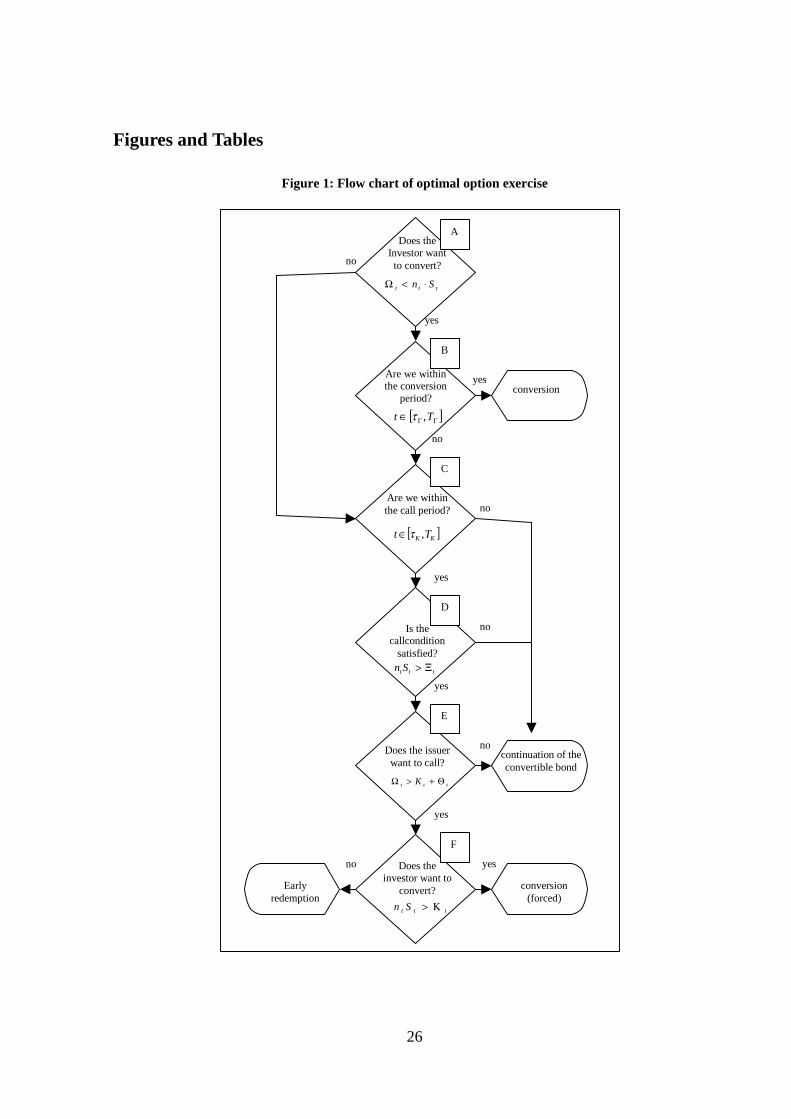
In each node, it is necessary to check whether each boundary condition is satisfied and to
determine the implications on the value of the convertible bond with respect to the optimal
calling behavior of the issuer and the optimal conversion behavior of the investor4.
Figure 1 shows a computationally efficient way of checking the validity of the boundary
conditions and the effects on the convertible bond. There are four possible outcomes: The
convertible bond continues to exist without being called or converted. Alternatively, it may be
called by the issuer, converted by the holder, or called by the issuer and subsequently
converted by the investor. The last scenario is often called forced conversion because the
investor is induced to convert exclusively by the fact that the issuer has called the bond.
When pricing convertible bonds, a dilution effect has to be taken into account. Because, in
most cases, new shares are created upon conversion, the equity value is divided among a
4 For a discussion on the optimal call and conversion policy, see Ingersoll (1977a).
Page 15
13
higher number of shares. This effect is mitigated (but not canceled) because the liabilities of
the firm are reduced as the convertible debt ceases to exist after conversion. In order to price
convertibles correctly, it is necessary to adjust the stock price in the model downwards.
Dilution is only relevant in the nodes A and F of the flow chart, when the investor decides to
convert. In this study, the dilution effect may be overestimated because we assume that the
green shoe option was always exercised in full when the bond was issued and that the bond is
always converted into newly issued stocks.
Integration of Credit Risk
The classical convertible bond pricing articles of Ingersoll (1977a) and Brennan and Schwartz
(1977) use the firm value as a stochastic variable. This approach allows for rigorous modeling
of credit risk and dilution but is very hard to implement empirically because the firm value is
not observable.
Ingersoll (1977a) and Brennan and Schwartz (1977) assume a simplistic capital structure,
consisting solely of equity and convertible bonds. In reality, such a capital structure is rather
rare. Brennan and Schwartz (1980) adapt the terminal and boundary conditions to cope with
the problem of the existence of senior debt. What seems an elegant way of solving the capital
structure problem in theory can be very hard to implement in practice. As a practical way of
solving this problem, King (1986) suggests to subtract the value of all senior debt positions
from the firm value and to assume this variable to follow geometric Brownian motion.
Unfortunately, this procedure does not take into account the stochastic character of the senior
debt. For convertible bonds of companies with relatively large senior debt issues, this pricing
procedure can be a rather rough approximation.
McConnell and Schwartz (1986) present a pricing model based on the stock value as
stochastic variable. Since the stock price cannot become negative, it is impossible to simulate
Page 16
14
bankruptcy scenarios. In other words, the model architecture is not capable of accounting for
credit risk in a natural way. However, convertible bonds are especially popular with lower-
rated issuers. Therefore, credit risk is a very important aspect of convertible bond pricing. To
account for credit risk, McConnell and Schwartz (1986) use an interest rate that is “grossed up
to capture the default risk of the issuer” (pp. 567) rather than the risk-free rate. This solution,
however, leaves open many questions about its quantification because the credit risk of a
convertible bond varies with respect to its moneyness.
For this reason, Tsiveriotis and Fernandes (1998) and Hull (2000) propose an approach that
splits the value of a convertible bond into a stock component and a straight bond component.
These two components belong to different credit risk categories. The former is risk-free
because a company is always able to deliver its own stock. The latter, however, is risky
because coupon and principal payments depend on the issuer’s capability of distributing the
required cash amounts. It is straightforward to discount the stock part of the convertible with
the risk-free interest rate and the straight bond component with a risk-adjusted rate. On the
contrary, the McConnell and Schwartz (1986) procedure produces a pooling between the two
components, as if the ratio of the two parts were constant. In reality, however, the relative
weight of the bond component can vary dramatically. On the one hand, when the convertible
bond is deep in the money, its value should be discounted using the risk-free rate. On the
other hand, when the bond is out of the money, the straight bond component is very high and
so is its defaultable part. This strategy is an improvement over the McConnell and Schwartz
(1986) approach because it clearly identifies the defaultable part of the convertible and thus
its credit risk exposure. We therefore adopt this approach in incorporating a constant
Page 17
15
exogenous credit spread into our binomial-tree model5. The appropriate credit spread is given
by the difference between the yield to maturity of a straight bond of the company and the
yield to maturity of a risk-free sovereign bond. The bonds have to be comparable, i.e. they
must have similar seniority, coupon and maturity. If no straight bond comparable to the
convertible exists, the credit spread can be estimated using the rating of the issuing firm.
Data
Convertible Bonds
Because convertible bonds are often traded over-the-counter, finding reliable time series of
market prices can be difficult. Even when electronic systems are in use, the delivered prices
are often not the quotes at which the actual trades occur. Additionally, synchronic market
prices of the stocks for which the convertible bonds can be exchanged are needed for this
study. We found these data requirements best satisfied for the French market. Moreover, the
French convertible bond market is one the most liquid European convertible bond markets
with a fair number of large convertible bond issues. We therefore chose the French market for
this pricing study.
We consider all French convertible bonds outstanding as of August 5, 2000. Daily convertible
bond prices as well as the corresponding synchronic stock prices are available from February
19, 1999, through August 5, 2000.6
5 It could be argued that credit risk increases with decreasing stock price. Since our credit spread is assumed to be constant, our model does
not take this negative correlation into account.
6 Data source: Mace Advisers.
Page 18
16
To exclude illiquid issues from the sample, we require every issue to satisfy three conditions
cumulatively7:
- a minimum market capitalisation of USD 75 million,
- a minimum average exchange traded volume reported to Autex for the last two quarters of
the equivalent of USD 75 million,
- at least three market makers out of the top ten convertible underwriters quoting prices
with a maximum bid/ask spread of 2 percentage points.
In addition, cross-currency convertibles are excluded from the sample. As a result, our
convertible bond universe consists of 21 French franc/euro-denominated issues with a total of
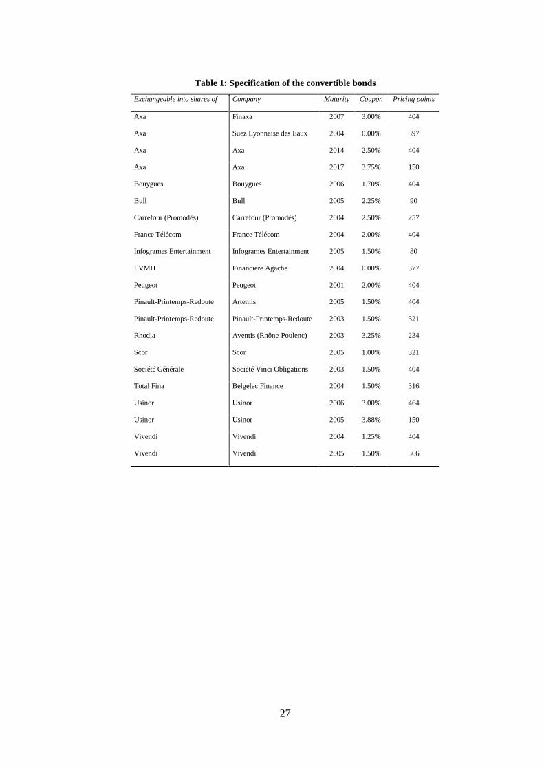
6760 data points. Table 1 gives an overview of the analyzed convertible bonds. All the
contractual specifications are extracted from the official and legally binding „offering
circulars“. This proved to be necessary because almost every electronic database tends to
suffer from an over-standardization syndrome. Although most bonds in our sample have very
similar specifications, some contractual provisions are so specific that they can hardly be
collected in predefined data types.
Several convertibles in our sample are “premium redemption” convertibles, i.e. the
redemption at maturity is above par value. In this case, the final redemption is given by κN
with the final redemption ratio κ greater than 1.
In the analyzed sample, there are seven exchangeable bonds. In these cases, the issuing firm
and the firm into the stock of which the bond can be converted are not the same firms.
7 These requirements are the same that UBS Warburg utilizes as exit criteria for its convertible bond index family.
Page 19
17
20 of the 21 analyzed convertibles include a call option, allowing the issuer to repurchase the
bond for a certain price Kt, called “call price” or “early redemption price”. This price varies
over time. Usually, the call price Kt is determined in such a way that the holder of the bond
obtains a similar return as when holding the convertible bond until maturity without
converting.
For almost all examined convertibles, early redemption is restricted to a certain predetermined
period from τK to TK. The period during which callability is not allowed is called the “call
protection period“. An additional restriction to callability in form of a supplementary
condition to be satisfied is given by the “call condition”. Callability is only allowed if the
parity ntSt exceeds a “call trigger” Ξt8. The call trigger is calculated as a percentage of either
the early redemption price or the face value (see Table 2). The last column shows, for each
bond, which of the two methods applies. If the trigger feature is present, the callability is
called “provisional” or “soft” call, if it is absent the callability is “absolute” or
“unconditional”. For almost all convertibles, the trigger feature is present. Only the bond
issued by Suez Lyonnaise des Eaux lacks a trigger and has an unconditional callability.
Another special case is Infograme Entertainment, which has a time-varying call trigger:
Within the period from May 30, 2000, to June 30, 2003, the call trigger is set at 250% of the
early redemption price. After July 1, 2003, the call trigger is reduced to 125% of the early
redemption price. For calculation in the binomial-tree model, we use the latter value.
Consequently, the model price may underestimate the fair value of this particular convertible
bond.
8 The exact contractual specification of the call condition often states that the inequality ntSt>Ξt must hold for a certain time (often 30 days)
before the bond becomes callable. This “qualifying period” introduces a path dependent feature not considered in the analysis.
Page 20
18
Usually, the conversion ratio tn is constant over time. It changes in case of an alteration of the
nominal value of the shares (stock subdivisions or consolidations), extraordinary dividend
payments and other financial operations that directly affect the stock price.
Conversion is possible within a certain period, called conversion period. The conversion
period starts at time τΓ and ends at time TΓ. For all the issues in our sample, the end of the
conversion period coincides with the maturity of the convertible bond, i.e. TΓ = T.
Dilution has been calculated on the basis of the number of shares outstanding9 and the number
of bonds to be issued as specified in the offering circulars. In twelve cases a “green shoe”
option was present, allowing the underwriter to increase the overall number of bonds. Because
we do not have any information regarding the exercise of the green shoe, we use the
maximum number of bonds (green shoe fully exercised) to estimate the dilution effect. Table
2 exhibits the number of bonds issued and the size of the green shoe option.
Interest Rates
For interest rates of one year or less (7 days, 1, 2, 3, 6, 12 months), we use Eurofranc rates10.
For longer maturities (1-10 years), we extract spot rates from swap rates using the standard
procedure. We observed that the one-year Eurofranc rate was systematically lower than the
corresponding one-year swap rate. Under the assumption that the Eurofranc rates represent a
better proxy for the theoretical credit risk-free rates, we adjust down the swap-extracted term
structure by the difference between the one-year Eurofranc rate and the one-year swap rate.
Furthermore, we use linear interpolation to obtain the complete continuous term structure of
spot rates.
9 Data source: Primark Datastream.
Page 21
19
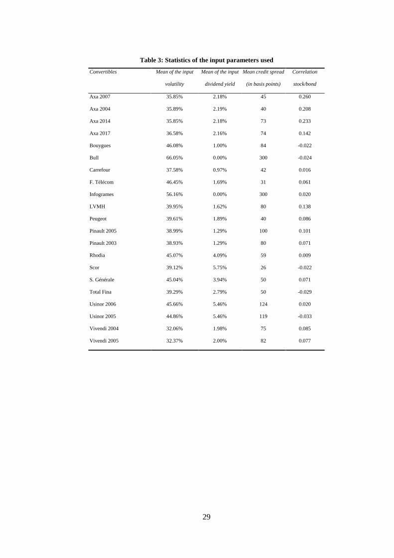
Unobservable Parameters
Besides directly observable input parameters, such as stock prices and interest rates, the
pricing models require input parameters that have to be estimated and thus are a source of
estimation error. These variables include volatility, dividends, correlations and credit spreads.
The most important input parameter to be estimated is the volatility of the underlying stock
price. Research on stock volatility estimation is plentiful. A popular approach is the implied
volatility concept. With option pricing formulas, it is possible to extract market participants’
volatility estimations from at-the-money option prices. However, most liquid options have
shorter maturities than convertibles. We therefore estimate volatility on a historical basis. The
relevant volatility is calculated as the standard deviation of the returns of the last 520 trading
days.
We model future dividends using a continuously compounded dividend yield. More precisely,
we assume that the best estimator for future dividends is the ratio of the current dividend11
level and the stock price. Furthermore, we assume that this ratio is constant over time.
The Margrabe model requires the correlation between the straight bond and the stock as an
input variable. Unfortunately, straight bonds with the same characteristics (coupon, maturity,
seniority) as the convertible bond are very rarely available. For this reason, we calculate the
correlation using time series of stock price and the theoretical investment value. The
investment value denotes the value of the convertible bond under the hypothetical assumption
that the conversion option does not exist.
10 All interest rate data is obtained from Primark Datastream.
11 Dividend information is obtained from Primark Datastream.
Page 22
20
Table 1 shows the mean credit spread expressed in basis points over the relevant period12.
Where the issuer has straight debt in the market, the credit spread is calculated on the basis of
the traded yield spread. Otherwise, it is calculated on the basis of credit spread indices, e.g.
the Bloomberg Fair Market Curves and UBS Credit Indices, according to the characteristics
of the sector in the relevant rating category.
Results
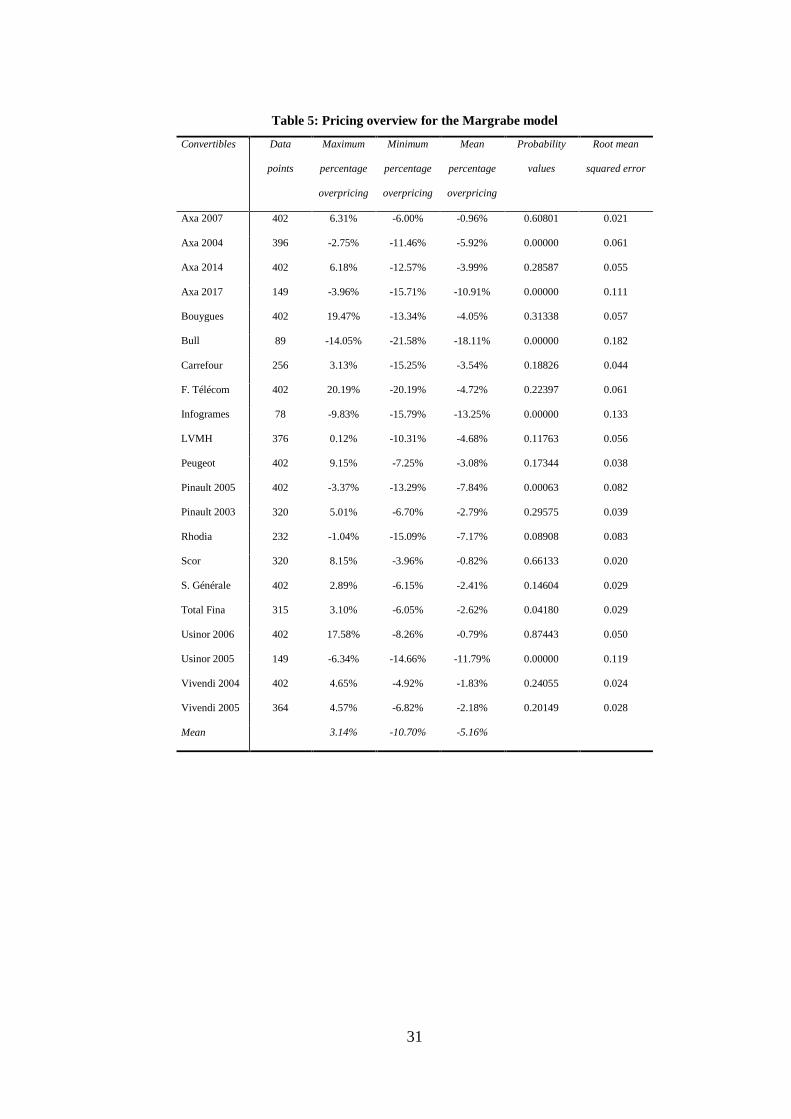
The observed convertible bond prices on the French market are compared with theoretical
prices obtained with three convertible bond pricing models. The main results of the three
implemented models are summarized13 in Table 4, Table 5, and Table 6. In analogy to the
methodology used by Sterk (1982) and others to test option pricing formulas, the tables
provide data about the maximum, minimum and mean percentage overpricing of each issue.
The mean percentage overpricing is presented for each convertible bond as an average of the
deviation between the theoretical and observed price for each observation. A negative value
indicates an underpricing, i.e. the theoretical value is above the observed market price.
Additionally, the probability values of a test for the null hypothesis of a mean overpricing of
zero are presented for each convertible. The last column shows the root mean squared error of
the relative mispricing. The RMSE shows the non-central standard deviation of the relative
deviations of model prices from market prices. It can be interpreted as a measure for the
pricing fit of the model relative to market prices.
With all three models, we observe on average substantially lower market prices than
theoretical prices. We obtain the largest underpricing for the component model (-8.74%),
12 We thank Rupert Kenna, credit analyst at UBS Warburg in London, for providing the daily credit spread time series.
13 Pricing results for each individual convertible bond are graphically displayed in the appendix.
Page 23
21
followed by the Margrabe model (-5.60%). The binomial-tree model is closest to the market
prices, but exhibits an average underpricing of -2.78%. This underpricing prevails even
though we value the convertible bond conservatively by assuming maximum dilution and
setting the safety premium to zero. For almost all convertibles, the binomial-tree model
produces the lowest theoretical price, followed by the Margrabe and the component model.
The only exception is the LVMH-convertible, where the overvaluation detected by the
Margrabe model is slightly higher than that of the binomial-tree model.
The binomial-tree model is the only model that in the entire sample detects cases of
overpricing. Among those five cases, the overpricing ranges from 3.78% (Usinor 2006) to
0.47% (Vivendi 2005). However, the mispricing is not significantly different from zero at a
five percent level. In contrast, sixteen convertible bonds have a mean percentage
underpricing. The significance test indicates that the mean price deviation of five of them is
significantly different from zero. Even though the overall theoretical pricing of the binomial-
tree model is close to the market data, the maximum and minimum percentage overpricing for
each convertible that occurred during the observation period often is very different. In some
cases, this may be caused by data outliers, which have not been removed in this study.
Prices calculated with the Margrabe model are substantially higher than both market prices
and theoretical binomial-tree prices, representing an underpricing for each convertible bond.
This can be explained by the fact that the model does not account for the call feature, which is
present in all but one of the examined convertible bonds. Callability reduces the stock-driven
upward-potential and thus has a negative impact on convertible prices.
For the component model, the mean percentage deviations from market prices are
significantly different from zero for 16 of the 21 convertible bonds, all of which are
overpriced by the model. Model prices are biased upwards because of two reasons: As in the
Page 24
22
Margrabe model, callability is neglected. Second, the strike price remains constant instead of
growing at a rate equal to the difference between interest rate and coupon. This distortion is
larger the longer the maturity of the bond and the lower the coupon rate is.
The fact that convertibles can be converted before maturity of the bond is accounted for
neither by the component model nor by the Margrabe model. This effect is of opposite
direction to the omission of the call feature. For eight convertibles in our sample, the dividend
yield is higher than the coupon rate. This is of interest, because it may make early conversion
optimal in a world of continuously compounded dividend yields and coupon rates.
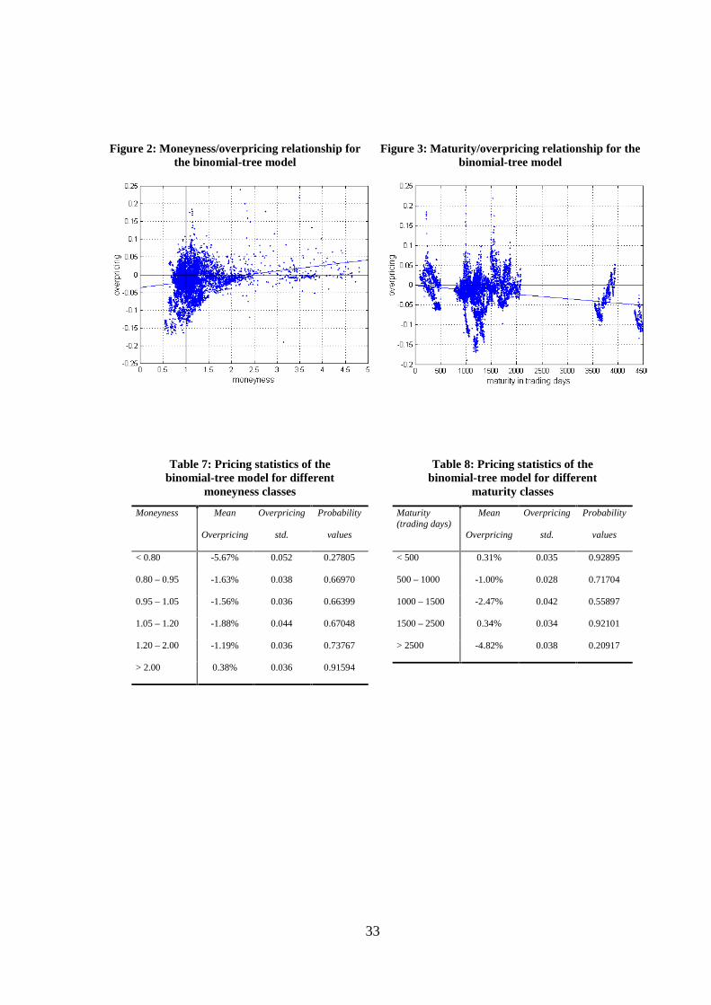
Figure 2 exhibits the overpricing of the observed market prices as detected by the binomial-
tree model plotted against the moneyness. The relationship is non-linear. The model
overprices bonds that are at-the-money and out-of-the money and underprices in-the-money
convertibles. These results are similar to those obtained by Carayannopoulos (1996). There
seems to be a slight relationship between overpricing and maturity (see Figure 3). The longer
the time to maturity, the more convertibles tend to be underpriced. However, these results rely
heavily on only two bonds (Axa 2014 and Axa 2017) that have a maturity far longer than the
others.
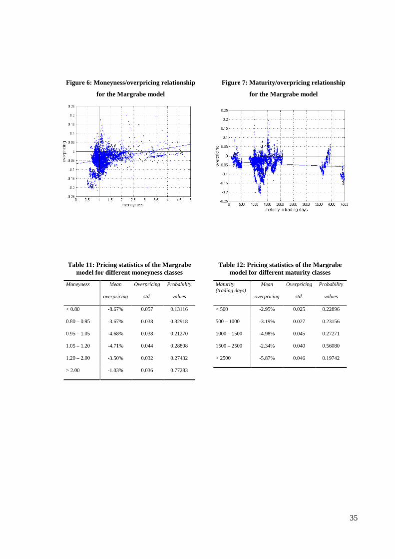
These results are similar for the other models. The relationship between overpricing and
moneyness is also positive. However, the relationship between overpricing and maturity is
slightly more negative for the component model. This finding is consistent with the above
mentioned fact that the component model tends to overprice bonds with long maturities and
with coupon rates below the interest rate level.
Page 25
23
Conclusion
We undertake a pricing study for the French convertible bond market. A simple component
model, a model based on exchange options, and a binomial-tree model are implemented.
Unlike the first two models, the binomial-tree model incorporates embedded options, dilution,
and credit risk. The model-generated prices are compared to the market prices of the
investigated convertible bonds using a sample of convertible bond prices of nearly 18 months
of daily data. For all three pricing models, on average, underpricing is detected. The results of
the binomial-tree model are closest to the market prices while the simple component model
has the greatest deviation. For all convertible bonds, the binomial-tree model gives the lowest
prices. Moreover, for the majority of bonds in our sample, the underpricing is not significant
for this model. A partition of the sample according to the moneyness indicates that the
underpricing is decreasing for bonds that are further in-the-money. Our findings of
underpricing, particularly for out-of-the-money bonds, are consistent with two previous
studies for the American market and anecdotal evidence from traders and other convertible
bond practitioners.
Page 26
24
References
BIS (2001), Bank for International Settlements Quarterly Review, March, pp. 71.
BLACK, F., and M. SCHOLES (1973): “The Pricing of Options and Corporate Liabilities”,
Journal of Political Economy, 81, 637-654.
BRENNAN, M.J., and E.S. SCHWARTZ (1977): “Convertible Bonds: Valuation and
Optimal Strategies for Call and Conversion”, The Journal of Finance, 32 (5), 1699-
1715.
BRENNAN, M.J., and E.S. SCHWARTZ (1980): “Analyzing Convertible Bonds”, Journal of
Financial and Quantitative Analysis, 15 (4), 907-929.
BUCHAN, J. (1997):”Convertible Bond Pricing: Theory and Evidence”, Unpublished
Dissertation, Harvard University.
BUCHAN, J. (1998):”The Pricing of Convertible Bonds with Stochastic Term Structures and
Corporate Default Risk”, Working Paper, Amos Tuck School of Business, Dartmouth
College.
CARAYANNOPOULOS, P. (1996): “Valuing Convertible Bonds under the Assumption of
Stochastic Interest Rates: An Empirical Investigation”, Quarterly Journal of Business
and Economics, 35 (3), 17-31.
COX, J.C., S.A. ROSS and M. RUBINSTEIN (1979): “Option Pricing: A simplified
Approach”, Journal of Financial Economics, 7 (3), 229-263.
HULL, J.C. (2000): Options, Futures & Other Derivatives. Prentice-Hall, Upper Saddle
River, N.Y., 4th ed.
Page 27
25
INGERSOLL, J.E. (1977a): “A Contingent Claim Valuation of Convertible Securities”,
Journal of Financial Economics, 4, 289-322.
INGERSOLL, J.E. (1977b): “An examination of corporate call policy on convertible
securities”, Journal of Finance, 32, 463-478.
KING, R. (1986): “Convertible Bond Valuation: An Empirical Test”, Journal of Financial
Research, 9 (1), 53-69.
MARGRABE, W (1978): “The Value of an Option to Exchange One Asset for Another”,
Journal of Finance, 33 (1), 177-186.
McCONNELL, J.J., and E.S. SCHWARTZ (1986): “LYON Taming”, The Journal of
Finance, 41 (3), 561-576.
STERK, W. (1982): “Tests of Two Models for Valuing Call Options on Stocks with
Dividends”, The Journal of Finance, 37 (5), 1229-1237.
SUBRAHMANYAM, M.G. (1990): “The Early Exercise Feature of American Options” in
FIGLEWSKI, S., W.L. SILBER and M.G. SUBRAHMANYAM (1990): “Financial
Options – From Theory to Practice”, Irwin, Burr Ridge, Illinois.
TSIVERIOTIS, K., and C. FERNANDES (1998): “Valuing Convertible Bonds with Credit
Risk”, The Journal of Fixed Income, 8 (3), 95-102.
Page 28
26
Figures and Tables
Figure 1: Flow chart of optimal option exercise
yes
no
yes
Does theInvestor want
to convert?
ttt Sn ⋅<Ω
Are we withinthe conversion
period?conversion
Are we withinthe call period?
[ ]KK Tt ,τ∈
Is thecallcondition
satisfied?
ttt Sn Ξ>
Does the issuerwant to call?
ttt K Θ+>Ω
Does theinvestor want to
convert?
ttt Sn Κ>
yes
no
yes
yes
yes
conversion(forced)
continuation of theconvertible bond
no
no
no
no
Earlyredemption
[ ]ΓΓ∈ Tt ,τ
A
B
C
F
E
D
Page 29
27
Table 1: Specification of the convertible bonds
Exchangeable into shares of Company Maturity Coupon Pricing points
Axa Finaxa 2007 3.00% 404
Axa Suez Lyonnaise des Eaux 2004 0.00% 397
Axa Axa 2014 2.50% 404
Axa Axa 2017 3.75% 150
Bouygues Bouygues 2006 1.70% 404
Bull Bull 2005 2.25% 90
Carrefour (Promodès) Carrefour (Promodès) 2004 2.50% 257
France Télécom France Télécom 2004 2.00% 404
Infogrames Entertainment Infogrames Entertainment 2005 1.50% 80
LVMH Financiere Agache 2004 0.00% 377
Peugeot Peugeot 2001 2.00% 404
Pinault-Printemps-Redoute Artemis 2005 1.50% 404
Pinault-Printemps-Redoute Pinault-Printemps-Redoute 2003 1.50% 321
Rhodia Aventis (Rhône-Poulenc) 2003 3.25% 234
Scor Scor 2005 1.00% 321
Société Générale Société Vinci Obligations 2003 1.50% 404
Total Fina Belgelec Finance 2004 1.50% 316
Usinor Usinor 2006 3.00% 464
Usinor Usinor 2005 3.88% 150
Vivendi Vivendi 2004 1.25% 404
Vivendi Vivendi 2005 1.50% 366
Page 30
28
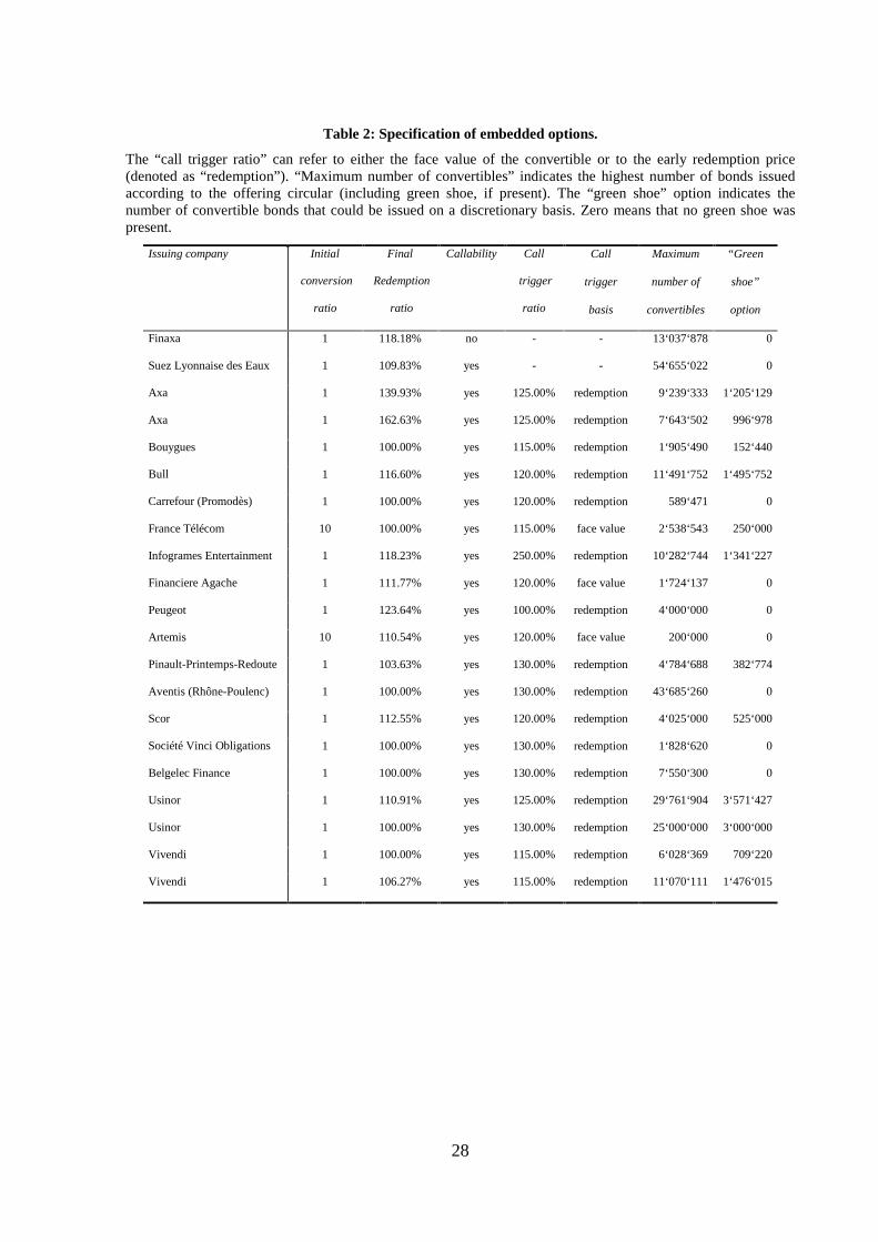
Table 2: Specification of embedded options.
The “call trigger ratio” can refer to either the face value of the convertible or to the early redemption price(denoted as “redemption”). “Maximum number of convertibles” indicates the highest number of bonds issuedaccording to the offering circular (including green shoe, if present). The “green shoe” option indicates thenumber of convertible bonds that could be issued on a discretionary basis. Zero means that no green shoe waspresent.
Issuing company Initial
conversion
ratio
Final
Redemption
ratio
Callability Call
trigger
ratio
Call
trigger
basis
Maximum
number of
convertibles
“Green
shoe”
option
Finaxa 1 118.18% no - - 13‘037‘878 0
Suez Lyonnaise des Eaux 1 109.83% yes - - 54‘655‘022 0
Axa 1 139.93% yes 125.00% redemption 9‘239‘333 1‘205‘129
Axa 1 162.63% yes 125.00% redemption 7‘643‘502 996‘978
Bouygues 1 100.00% yes 115.00% redemption 1‘905‘490 152‘440
Bull 1 116.60% yes 120.00% redemption 11‘491‘752 1‘495‘752
Carrefour (Promodès) 1 100.00% yes 120.00% redemption 589‘471 0
France Télécom 10 100.00% yes 115.00% face value 2‘538‘543 250‘000
Infogrames Entertainment 1 118.23% yes 250.00% redemption 10‘282‘744 1‘341‘227
Financiere Agache 1 111.77% yes 120.00% face value 1‘724‘137 0
Peugeot 1 123.64% yes 100.00% redemption 4‘000‘000 0
Artemis 10 110.54% yes 120.00% face value 200‘000 0
Pinault-Printemps-Redoute 1 103.63% yes 130.00% redemption 4‘784‘688 382‘774
Aventis (Rhône-Poulenc) 1 100.00% yes 130.00% redemption 43‘685‘260 0
Scor 1 112.55% yes 120.00% redemption 4‘025‘000 525‘000
Société Vinci Obligations 1 100.00% yes 130.00% redemption 1‘828‘620 0
Belgelec Finance 1 100.00% yes 130.00% redemption 7‘550‘300 0
Usinor 1 110.91% yes 125.00% redemption 29‘761‘904 3‘571‘427
Usinor 1 100.00% yes 130.00% redemption 25‘000‘000 3‘000‘000
Vivendi 1 100.00% yes 115.00% redemption 6‘028‘369 709‘220
Vivendi 1 106.27% yes 115.00% redemption 11‘070‘111 1‘476‘015
Page 31
29
Table 3: Statistics of the input parameters used
Convertibles Mean of the input
volatility
Mean of the input
dividend yield
Mean credit spread
(in basis points)
Correlation
stock/bond
Axa 2007 35.85% 2.18% 45 0.260
Axa 2004 35.89% 2.19% 40 0.208
Axa 2014 35.85% 2.18% 73 0.233
Axa 2017 36.58% 2.16% 74 0.142
Bouygues 46.08% 1.00% 84 -0.022
Bull 66.05% 0.00% 300 -0.024
Carrefour 37.58% 0.97% 42 0.016
F. Télécom 46.45% 1.69% 31 0.061
Infogrames 56.16% 0.00% 300 0.020
LVMH 39.95% 1.62% 80 0.138
Peugeot 39.61% 1.89% 40 0.086
Pinault 2005 38.99% 1.29% 100 0.101
Pinault 2003 38.93% 1.29% 80 0.071
Rhodia 45.07% 4.09% 59 0.009
Scor 39.12% 5.75% 26 -0.022
S. Générale 45.04% 3.94% 50 0.071
Total Fina 39.29% 2.79% 50 -0.029
Usinor 2006 45.66% 5.46% 124 0.020
Usinor 2005 44.86% 5.46% 119 -0.033
Vivendi 2004 32.06% 1.98% 75 0.085
Vivendi 2005 32.37% 2.00% 82 0.077
Page 32
30
Table 4: Pricing overview for the binomial-tree model
“Data points” indicates the number of days for which model prices are computed. “Probability values” is a twosided test for the H0 hypothesis that model prices and observed prices are equal in the mean. The “root meansquared error” is the non-central standard deviation of the relative deviations of model prices from market prices.
Convertibles Data
points
Maximum
percentage
overpricing
Minimum
percentage
overpricing
Mean
percentage
overpricing
Probability
values
Root mean
squared error
Axa 2007 402 5.83% -5.42% -0.58% 0.72974 0.018
Axa 2004 396 4.23% -7.56% -0.56% 0.77267 0.020
Axa 2014 402 5.19% -10.08% -3.37% 0.31523 0.048
Axa 2017 149 -2.55% -13.34% -8.71% 0.00000 0.089
Bouygues 402 21.84% -9.76% -1.40% 0.68053 0.037
Bull 89 -9.75% -16.81% -14.07% 0.00000 0.142
Carrefour 256 7.99% -10.87% 1.46% 0.59718 0.031
F. Télécom 402 23.92% -18.97% -1.60% 0.66270 0.040
Infogrames 78 -8.49% -14.36% -11.72% 0.00000 0.118
LVMH 376 -0.62% -9.65% -4.76% 0.06953 0.054
Peugeot 402 18.39% -2.78% 2.46% 0.31557 0.035
Pinault 2005 402 0.00% -8.67% -3.73% 0.04404 0.042
Pinault 2003 320 5.41% -6.40% -2.39% 0.37238 0.036
Rhodia 232 0.32% -13.00% -5.40% 0.17815 0.067
Scor 320 9.88% -2.67% 0.67% 0.72626 0.020
S. Générale 402 3.74% -5.19% -1.61% 0.30344 0.022
Total Fina 315 3.64% -4.82% -1.60% 0.18626 0.020
Usinor 2006 402 17.51% -4.51% 3.78% 0.18799 0.047
Usinor 2005 149 -3.51% -11.11% -8.13% 0.00000 0.082
Vivendi 2004 402 6.64% -3.83% -0.28% 0.86665 0.017
Vivendi 2005 364 7.66% -3.72% 0.47% 0.79780 0.019
Mean 5.33% -8.34% -2.78%
Page 33
31
Table 5: Pricing overview for the Margrabe model
Convertibles Data
points
Maximum
percentage
overpricing
Minimum
percentage
overpricing
Mean
percentage
overpricing
Probability
values
Root mean
squared error
Axa 2007 402 6.31% -6.00% -0.96% 0.60801 0.021
Axa 2004 396 -2.75% -11.46% -5.92% 0.00000 0.061
Axa 2014 402 6.18% -12.57% -3.99% 0.28587 0.055
Axa 2017 149 -3.96% -15.71% -10.91% 0.00000 0.111
Bouygues 402 19.47% -13.34% -4.05% 0.31338 0.057
Bull 89 -14.05% -21.58% -18.11% 0.00000 0.182
Carrefour 256 3.13% -15.25% -3.54% 0.18826 0.044
F. Télécom 402 20.19% -20.19% -4.72% 0.22397 0.061
Infogrames 78 -9.83% -15.79% -13.25% 0.00000 0.133
LVMH 376 0.12% -10.31% -4.68% 0.11763 0.056
Peugeot 402 9.15% -7.25% -3.08% 0.17344 0.038
Pinault 2005 402 -3.37% -13.29% -7.84% 0.00063 0.082
Pinault 2003 320 5.01% -6.70% -2.79% 0.29575 0.039
Rhodia 232 -1.04% -15.09% -7.17% 0.08908 0.083
Scor 320 8.15% -3.96% -0.82% 0.66133 0.020
S. Générale 402 2.89% -6.15% -2.41% 0.14604 0.029
Total Fina 315 3.10% -6.05% -2.62% 0.04180 0.029
Usinor 2006 402 17.58% -8.26% -0.79% 0.87443 0.050
Usinor 2005 149 -6.34% -14.66% -11.79% 0.00000 0.119
Vivendi 2004 402 4.65% -4.92% -1.83% 0.24055 0.024
Vivendi 2005 364 4.57% -6.82% -2.18% 0.20149 0.028
Mean 3.14% -10.70% -5.16%
Page 34
32
Table 6: Pricing overview for the component model
Convertibles Data
points
Maximum
percentage
overpricing
Minimum
percentage
overpricing
Mean
percentage
overpricing
Probability
values
Root mean
squared error
Axa 2007 402 1.36% -10.58% -5.53% 0.00189 0.058
Axa 2004 396 -6.72% -17.15% -11.05% 0.00000 0.112
Axa 2014 402 -0.52% -19.66% -11.20% 0.00647 0.119
Axa 2017 149 -8.29% -19.40% -14.88% 0.00000 0.150
Bouygues 402 15.16% -17.60% -8.09% 0.06020 0.092
Bull 89 -17.43% -24.66% -21.23% 0.00000 0.213
Carrefour 256 0.49% -18.00% -6.54% 0.01473 0.071
F. Télécom 402 16.62% -22.40% -7.43% 0.03818 0.083
Infogrames 78 -16.04% -21.52% -19.05% 0.00000 0.191
LVMH 376 -6.49% -14.25% -10.41% 0.00001 0.107
Peugeot 402 7.72% -8.48% -4.28% 0.06345 0.049
Pinault 2005 402 -5.69% -17.89% -11.67% 0.00009 0.120
Pinault 2003 320 3.51% -7.97% -4.18% 0.09978 0.049
Rhodia 232 -2.47% -16.11% -8.51% 0.03784 0.094
Scor 320 2.67% -8.51% -5.36% 0.00267 0.056
S. Générale 402 1.43% -8.67% -5.00% 0.00891 0.054
Total Fina 315 -1.52% -8.82% -6.24% 0.00000 0.064
Usinor 2006 402 13.40% -11.32% -3.92% 0.40018 0.061
Usinor 2005 149 -7.93% -15.55% -12.99% 0.00000 0.131
Vivendi 2004 402 -0.95% -10.13% -6.45% 0.00002 0.066
Vivendi 2005 364 -1.70% -11.02% -7.71% 0.00000 0.078
Mean -0.61% -14.08% -8.71%
Page 35
33
Figure 2: Moneyness/overpricing relationship forthe binomial-tree model
Figure 3: Maturity/overpricing relationship for thebinomial-tree model
Table 7: Pricing statistics of thebinomial-tree model for different
moneyness classes
Moneyness Mean
Overpricing
Overpricing
std.
Probability
values
< 0.80 -5.67% 0.052 0.27805
0.80 – 0.95 -1.63% 0.038 0.66970
0.95 – 1.05 -1.56% 0.036 0.66399
1.05 – 1.20 -1.88% 0.044 0.67048
1.20 – 2.00 -1.19% 0.036 0.73767
> 2.00 0.38% 0.036 0.91594
Table 8: Pricing statistics of thebinomial-tree model for different
maturity classes
Maturity(trading days)
Mean
Overpricing
Overpricing
std.
Probability
values
< 500 0.31% 0.035 0.92895
500 – 1000 -1.00% 0.028 0.71704
1000 – 1500 -2.47% 0.042 0.55897
1500 – 2500 0.34% 0.034 0.92101
> 2500 -4.82% 0.038 0.20917
Page 36
34
Figure 4: Moneyness/overpricing relationship
for the component model
Figure 5: Maturity/overpricing relationship
for the component model
Table 9: Pricing statistics of the componentmodel for different moneyness classes
Moneyness Mean
overpricing
Overpricing
std.
Probability
values
< 0.80 -10.35% 0.062 0.09389
0.80 – 0.95 -7.19% 0.038 0.05918
0.95 – 1.05 -7.94% 0.040 0.04975
1.05 – 1.20 -8.70% 0.051 0.09094
1.20 – 2.00 -8.03% 0.038 0.03423
> 2.00 -4.89% 0.035 0.16323
Table 10: Pricing statistics of the componentmodel for different maturity classes
Maturity(trading days)
Mean
overpricing
Overpricing
std.
Probability
values
< 500 -4.24% 0.024 0.07898
500 – 1000 -6.69% 0.029 0.01996
1000 – 1500 -9.02% 0.044 0.03819
1500 – 2500 -6.16% 0.040 0.12380
> 2500 -12.20% 0.040 0.00227
Page 37
35
Figure 6: Moneyness/overpricing relationship
for the Margrabe model
Figure 7: Maturity/overpricing relationship
for the Margrabe model
Table 11: Pricing statistics of the Margrabemodel for different moneyness classes
Moneyness Mean
overpricing
Overpricing
std.
Probability
values
< 0.80 -8.67% 0.057 0.13116
0.80 – 0.95 -3.67% 0.038 0.32918
0.95 – 1.05 -4.68% 0.038 0.21270
1.05 – 1.20 -4.71% 0.044 0.28808
1.20 – 2.00 -3.50% 0.032 0.27432
> 2.00 -1.03% 0.036 0.77283
Table 12: Pricing statistics of the Margrabemodel for different maturity classes
Maturity(trading days)
Mean
overpricing
Overpricing
std.
Probability
values
< 500 -2.95% 0.025 0.22896
500 – 1000 -3.19% 0.027 0.23156
1000 – 1500 -4.98% 0.045 0.27271
1500 – 2500 -2.34% 0.040 0.56080
> 2500 -5.87% 0.046 0.19742
Page 38
36
Appendix
0 50 100 150 200 250 300 350 400 45060
80
100
120
140
160
180
trading days
valu
es
pricing of the Axa 2007, 3% convertible
theoretical fair valueempirical value parity investment value
0 50 100 150 200 250 300 350 400 450-0.06
-0.04
-0.02
0
0.02
0.04
0.06
trading days
ove
rva
luat
ion
percentage overvaluation of the Axa 2007, 3% convertible
0 50 100 150 200 250 300 350 400100
110
120
130
140
150
160
170
180
190
trading days
valu
es
pricing of the Axa 2004, 0% convertible
theoretical fair valueempirical value parity investment value
0 50 100 150 200 250 300 350 400-0.08
-0.06
-0.04
-0.02
0
0.02
0.04
0.06
trading days
ove
rva
luat
ion
percentage overvaluation of the Axa 2004, 0% convertible
0 50 100 150 200 250 300 350 400 450100
110
120
130
140
150
160
170
180
190
200
trading days
valu
es
pricing of the Axa 2014, 2.5% convertible
theoretical fair valueempirical value parity investment value
0 50 100 150 200 250 300 350 400 450-0.12
-0.1
-0.08
-0.06
-0.04
-0.02
0
0.02
0.04
0.06
trading days
ove
rva
luat
ion
percentage overvaluation of the Axa 2014, 2.5% convertible
0 50 100 150120
130
140
150
160
170
180
190
200
210
220
trading days
valu
es
pricing of the Axa 2017, 3.75% convertible
theoretical fair valueempirical value parity investment value
0 50 100 150-0.14
-0.12
-0.1
-0.08
-0.06
-0.04
-0.02
trading days
ove
rva
luat
ion
percentage overvaluation of the Axa 2017, 3.75% convertible
Page 39
37
0 50 100 150 200 250 300 350 400 450100
200
300
400
500
600
700
800
900
1000
trading days
valu
espricing of the Bouygues 2006, 1.7% convertible
theoretical fair valueempirical value parity investment value
0 50 100 150 200 250 300 350 400 450-0.1
-0.05
0
0.05
0.1
0.15
0.2
0.25
trading days
ove
rva
luat
ion
percentage overvaluation of the Bouygues 2006, 1.7% convertible
0 10 20 30 40 50 60 70 80 906
8
10
12
14
16
18
20
trading days
valu
es
pricing of the Bull 2005, 2.25% convertible
theoretical fair valueempirical value parity investment value
0 10 20 30 40 50 60 70 80 90-0.17
-0.16
-0.15
-0.14
-0.13
-0.12
-0.11
-0.1
-0.09
trading days
ove
rva
luat
ion
percentage overvaluation of the Bull 2005, 2.25% convertible
0 50 100 150 200 250 300700
800
900
1000
1100
1200
1300
trading days
valu
es
pricing of the Carrefour 2004, 2.5% convertible
theoretical fair valueempirical value parity investment value
0 50 100 150 200 250 300-0.12
-0.1
-0.08
-0.06
-0.04
-0.02
0
0.02
0.04
0.06
0.08
trading days
ove
rva
luat
ion
percentage overvaluation of the Carrefour 2004, 2.5% convertible
0 50 100 150 200 250 300 350 400 450600
800
1000
1200
1400
1600
1800
2000
2200
trading days
valu
es
pricing of the France Télécom 2004, 2% convertible
theoretical fair valueempirical value parity investment value
0 50 100 150 200 250 300 350 400 450-0.2
-0.15
-0.1
-0.05
0
0.05
0.1
0.15
0.2
0.25
trading days
ove
rva
luat
ion
percentage overvaluation of the France Télécom 2004, 2% convertible
Page 40
38
0 10 20 30 40 50 60 70 8020
25
30
35
40
45
50
trading days
valu
es
pricing of the Infogrames Entertainment 2005, 1.5% convertible
theoretical fair valueempirical value parity investment value
0 10 20 30 40 50 60 70 80-0.15
-0.14
-0.13
-0.12
-0.11
-0.1
-0.09
-0.08
trading days
ove
rva
luat
ion
percentage overvaluation of the Infogrames Entertainment 2005, 1.5% convertible
0 50 100 150 200 250 300 350 400200
250
300
350
400
450
500
550
trading days
valu
es
pricing of the LVMH 2004, 0% convertible
theoretical fair valueempirical value parity investment value
0 50 100 150 200 250 300 350 400-0.1
-0.09
-0.08
-0.07
-0.06
-0.05
-0.04
-0.03
-0.02
-0.01
0
trading days
ove
rva
luat
ion
percentage overvaluation of the LVMH 2004, 0% convertible
0 50 100 150 200 250 300 350 400 450100
150
200
250
trading days
valu
es
pricing of the Peugeot 2001, 2% convertible
theoretical fair valueempirical value parity investment value
0 50 100 150 200 250 300 350 400 450-0.05
0
0.05
0.1
0.15
0.2
trading days
ove
rva
luat
ion
percentage overvaluation of the Peugeot 2001, 2% convertible
0 50 100 150 200 250 300 350 400 4501200
1400
1600
1800
2000
2200
2400
2600
2800
3000
trading days
valu
es
pricing of the Pinault-Printemps 2005, 1.5% convertible
theoretical fair valueempirical value parity investment value
0 50 100 150 200 250 300 350 400 450-0.09
-0.08
-0.07
-0.06
-0.05
-0.04
-0.03
-0.02
-0.01
0
0.01
trading days
ove
rva
luat
ion
percentage overvaluation of the Pinault-Printemps 2005, 1.5% convertible
Page 41
39
0 50 100 150 200 250 300 350140
160
180
200
220
240
260
280
300
trading days
valu
espricing of the Pinault-Printemps 2003, 1.5% convertible
theoretical fair valueempirical value parity investment value
0 50 100 150 200 250 300 350-0.08
-0.06
-0.04
-0.02
0
0.02
0.04
0.06
trading days
ove
rva
luat
ion
percentage overvaluation of the Pinault-Printemps 2003, 1.5% convertible
0 50 100 150 200 25015
20
25
30
trading days
valu
es
pricing of the Rhodia 2003, 3.25% convertible
theoretical fair valueempirical value parity investment value
0 50 100 150 200 250-0.14
-0.12
-0.1
-0.08
-0.06
-0.04
-0.02
0
0.02
trading days
ove
rva
luat
ion
percentage overvaluation of the Rhodia 2003, 3.25% convertible
0 50 100 150 200 250 300 35040
45
50
55
60
65
trading days
valu
es
pricing of the Scor 2005, 1% convertible
theoretical fair valueempirical value parity investment value
0 50 100 150 200 250 300 350-0.04
-0.02
0
0.02
0.04
0.06
0.08
0.1
trading days
ove
rva
luat
ion
percentage overvaluation of the Scor 2005, 1% convertible
0 50 100 150 200 250 300 350 400 450120
140
160
180
200
220
240
260
280
300
trading days
valu
es
pricing of the Société Générale 2003, 1.5% convertible
theoretical fair valueempirical value parity investment value
0 50 100 150 200 250 300 350 400 450-0.06
-0.05
-0.04
-0.03
-0.02
-0.01
0
0.01
0.02
0.03
0.04
trading days
ove
rva
luat
ion
percentage overvaluation of the Société Générale 2003, 1.5% convertible
Page 42
40
0 50 100 150 200 250 300 350110
120
130
140
150
160
170
180
190
200
trading days
valu
espricing of the Total Fina 2004, 1.5% convertible
theoretical fair valueempirical value parity investment value
0 50 100 150 200 250 300 350-0.05
-0.04
-0.03
-0.02
-0.01
0
0.01
0.02
0.03
0.04
trading days
ove
rva
luat
ion
percentage overvaluation of the Total Fina 2004, 1.5% convertible
0 50 100 150 200 250 300 350 400 45010
12
14
16
18
20
22
trading days
valu
es
pricing of the Usinor 2006, 3% convertible
theoretical fair valueempirical value parity investment value
0 50 100 150 200 250 300 350 400 450-0.05
0
0.05
0.1
0.15
0.2
trading days
ove
rva
luat
ion
percentage overvaluation of the Usinor 2006, 3% convertible
0 50 100 15010
12
14
16
18
20
22
24
trading days
valu
es
pricing of the Usinor 2005, 3.875% convertible
theoretical fair valueempirical value parity investment value
0 50 100 150-0.12
-0.11
-0.1
-0.09
-0.08
-0.07
-0.06
-0.05
-0.04
-0.03
trading days
ove
rva
luat
ion
percentage overvaluation of the Usinor 2005, 3.875% convertible
0 50 100 150 200 250 300 350 400 450150
200
250
300
350
400
450
trading days
valu
es
pricing of the Vivendi 2004, 1.25% convertible
theoretical fair valueempirical value parity investment value
0 50 100 150 200 250 300 350 400 450-0.04
-0.02
0
0.02
0.04
0.06
0.08
trading days
ove
rva
luat
ion
percentage overvaluation of the Vivendi 2004, 1.25% convertible
Page 43
41
0 50 100 150 200 250 300 350 400150
200
250
300
350
400
450
trading days
valu
espricing of the Vivendi 2005, 1.5% convertible
theoretical fair valueempirical value parity investment value
0 50 100 150 200 250 300 350 400-0.04
-0.02
0
0.02
0.04
0.06
0.08
trading days
ove
rva
luat
ion
percentage overvaluation of the Vivendi 2005, 1.5% convertible