Ulm University Faculty of Mathematics and Economics The Prime Number Theorem Bachelor Thesis Business Mathematics submitted by Wiesel, Johannes on 05.07.2013 Referee Professor Wolfgang Arendt
Transcript
Ulm UniversityFaculty of Mathematics and Economics
The Prime Number Theorem
Bachelor Thesis
Business Mathematics
submitted byWiesel, Johannes
on 05.07.2013
Referee
Professor Wolfgang Arendt
Contents
1. A Historical Introduction 32. The Riemann Zeta Function and the Tschebyscheff Functions 63. Equivalences of the Prime Number Theorem 94. Partial Sums and some elementary results 115. An Auxiliary Tauberian Theorem 166. The Proof of the Prime Number Theorem 207. Immediate consequences of the Prime Number Theorem and Betrand’s
Postulate 278. Outlook on current developments 318.1. Maier’s Theorem: Primes in short intervals 318.2. Green-Tao’s Theorem: Primes contain arbitrarily long arithmetic
progessions 328.3. Helfgott: Minor and Major Arcs for Goldbach’s Problem 328.4. Zhang: Bounded gaps between primes 339. The Functional Equation of the Zeta Function 3410. The Riemann Hypothesis 43References 46List of Figures 47
3
1. A Historical Introduction
The Prime Number Theorem looks back on a remarkable history. It should takemore than 100 years from the first assumption of the theorem to its complete proofby analytic means. Before we give a detailed description of the historical events,let us first state what it is all about: The Prime Number Theorem says, that theasymptotic behaviour of the number of primes, which are smaller than some valuex, is roughly x/ log(x) for x→∞. This was assumed by 15-year old Carl FriedrichGauß1 in 1793 and by Adrien-Marie Legendre2 in 1798, but was not proven until1896, when Jacques Salomon Hadamard3 and Charles-Jean de la Vallee Poussin4
independently of each other found a way to approach this problem. The proof waslater simplified by many famous mathematicians. Amongst others Wiener, Landauand D.J. Newmann could make some important improvements.
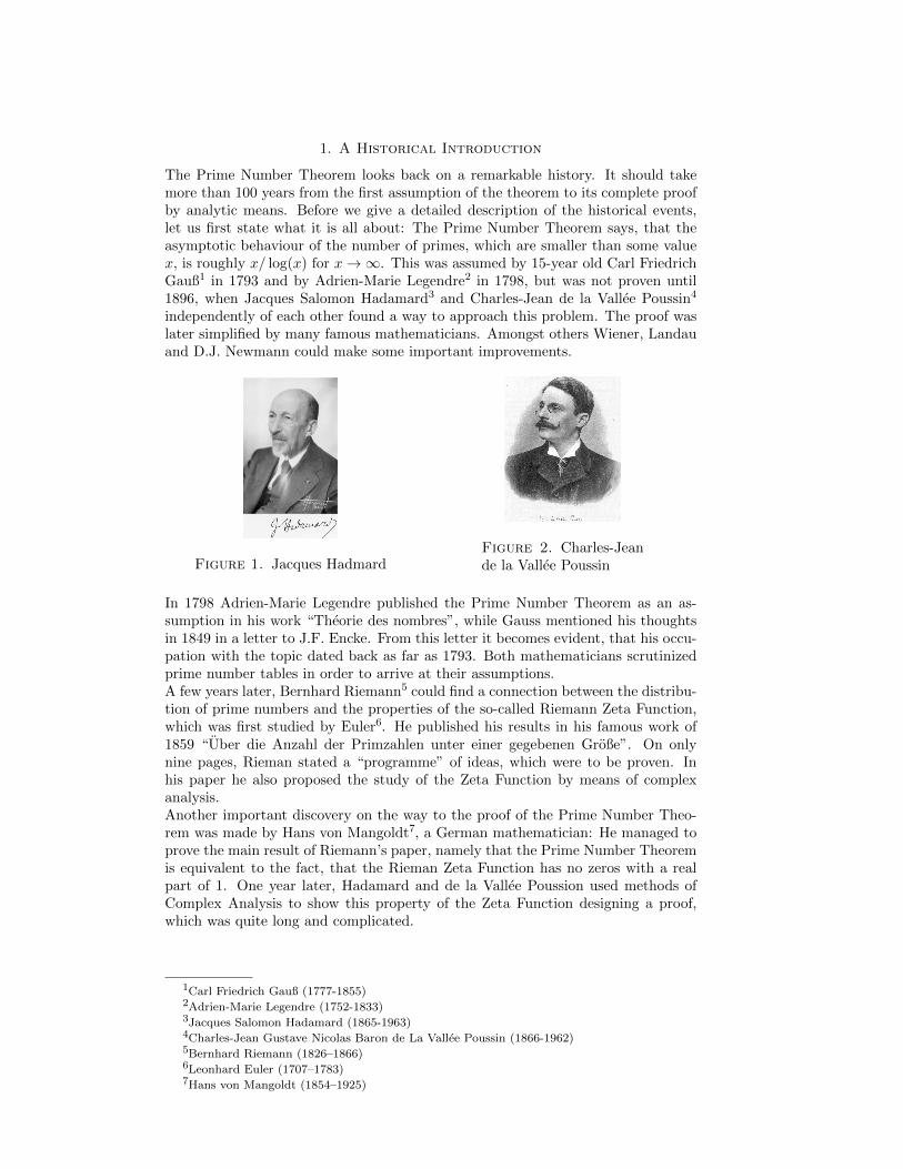
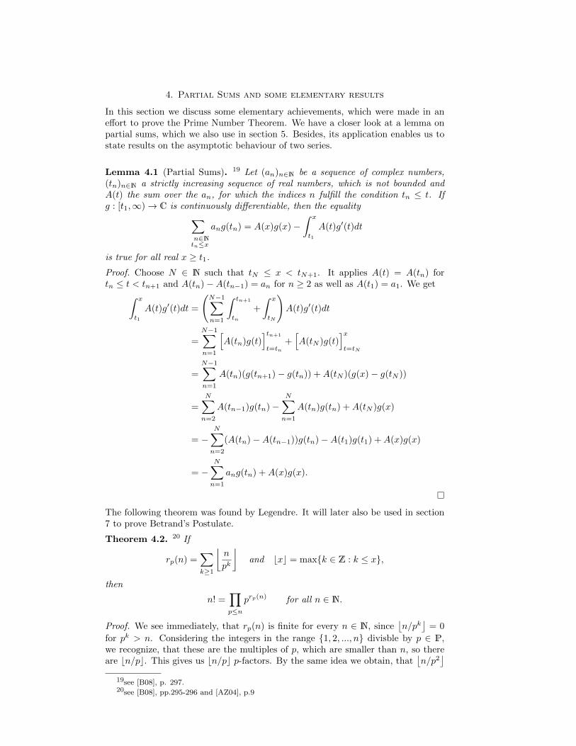
Figure 1. Jacques HadmardFigure 2. Charles-Jeande la Vallee Poussin
In 1798 Adrien-Marie Legendre published the Prime Number Theorem as an as-sumption in his work “Theorie des nombres”, while Gauss mentioned his thoughtsin 1849 in a letter to J.F. Encke. From this letter it becomes evident, that his occu-pation with the topic dated back as far as 1793. Both mathematicians scrutinizedprime number tables in order to arrive at their assumptions.A few years later, Bernhard Riemann5 could find a connection between the distribu-tion of prime numbers and the properties of the so-called Riemann Zeta Function,which was first studied by Euler6. He published his results in his famous work of1859 “Uber die Anzahl der Primzahlen unter einer gegebenen Große”. On onlynine pages, Rieman stated a “programme” of ideas, which were to be proven. Inhis paper he also proposed the study of the Zeta Function by means of complexanalysis.Another important discovery on the way to the proof of the Prime Number Theo-rem was made by Hans von Mangoldt7, a German mathematician: He managed toprove the main result of Riemann’s paper, namely that the Prime Number Theoremis equivalent to the fact, that the Rieman Zeta Function has no zeros with a realpart of 1. One year later, Hadamard and de la Vallee Poussion used methods ofComplex Analysis to show this property of the Zeta Function designing a proof,which was quite long and complicated.
1Carl Friedrich Gauß (1777-1855)2Adrien-Marie Legendre (1752-1833)3Jacques Salomon Hadamard (1865-1963)4Charles-Jean Gustave Nicolas Baron de La Vallee Poussin (1866-1962)5Bernhard Riemann (1826–1866)6Leonhard Euler (1707–1783)7Hans von Mangoldt (1854–1925)
4
Figure 3. BernhardRiemann
Figure 4. Don Zagier
For a long time, mathematicians also tried to find elementary proofs (i.e. proofs,which do not use Complex Analysis). In the time between 1851 and 1854, PafnutiTschebyscheff8 worked on a proof of the Prime Number Theorem and could make im-portant findings, which we will partially discuss here. Tschebyscheff also found lowerand upper bounds for the ratio of the prime counting function π(x) and x/ log(x)for sufficiently large values of x. However, it should still take some time, until thePrime Number Theorem could finally be proven by elementary means: Roughly 100years later, in 1949, the mathematicians Atle Selberg9 und Paul Erdos10 managedto solve this problem. Although the word elementary makes one suggest differ-ently, their proof is quite complicated. This discovery helped elementary methodsof Number Theory regain a good reputation in comparison to analytic methods, asthe German mathematician Carl Ludwig Siegel stated: ”This shows, that one can-not say anything about the real difficulties of a problem, before one has solved it.”11
The ideas and steps of the proof given here were stated by Don Bernard Zagier12
in his work ”Newman’s Short Proof of the Prime Number Theorem” of 1997. DonZagier follows the work of Donald J. Newman and Jacob Korevaar with a few sim-plifications.For the full understanding a basic knowledge of Complex Analysis is assumed.
We now introduce some basic definitions.
Definition 1.1. We define P as the set of all prime numbers and π(x) as thenumber of primes smaller or equal to x, i.e.
π(x) = |{p ∈ P : p ≤ x}| .
Definition 1.2. Let us define the integral logarithm
li(x) =
∫ x
2
1
log(t)dt.
Definition 1.3. We say two functions f, g : R→ R are asymptotically equal, if
limx→∞
f(x)
g(x)= 1
and write
f ∼ g (x→∞).
8Pafnuti Lwowitsch Tschebyscheff (1821-1894)9Atle Selberg (1917–2007)10Paul Erdos (1913–1996)11see [B08], p. 322.12Don Bernard Zagier (1951-)
5
Definition 1.4. We write for two functions f, g : R→ R
f = O(g) (x→∞),
if
∃C ∈ R ∃x0 > 0 ∀x > x0 : |f(x)| ≤ C|g(x)|.We write for a real number a <∞
f = O(g) (x→ a),
if
∃C ∈ R ∃ε > 0 ∀|x− a| < ε : |f(x)| ≤ C|g(x)|.
With these notations in mind, we state the Prime Number Theorem in the followingway:
Theorem 1.5 (Prime Number Theorem). The prime counting function π(x) isasysmptotically equal to the ratio x/ log x, i.e.
π(x) ∼ x
log x(x→∞).
6
2. The Riemann Zeta Function and the Tschebyscheff Functions
In this section we introduce the Riemann Zeta Function and the TschebyscheffFunctions. Besides, we take a first look at their properties. The Zeta Function wasfirst examined by Euler in the 18th century, before Riemann made some importantdiscoveries on its properties.
Definition 2.1. 13 We define the following functions, which are useful for the proofof the Prime Number Theorem. The p under the sigma sign means, that we sumover all p ∈ P.
Riemann Zeta Function: ζ(s) =∞∑n=1
1ns (Re (s) > 1)
Tschebyscheff Functions: φ(s) =∑p
log pps (Re (s) > 1)
ϑ(x) =∑p≤x
log p (x ∈ R)
Let us now take a closer look at the first two functions.
Lemma 2.2. 14 For Re (s) > 1, ζ(s) and φ(s) are normally convergent and thereforedefine holomorphic functions in that domain.
Proof. For δ > 0, n ∈ N and Re (s) ≥ 1 + δ, we obtain
|n−s| = |e−s logn| = n−Re (s) ≤ n−(1+δ).
The series∑∞n=1
1n1+δ is convergent, so the Zeta Function converges normally and
is hence holomorphic on {s ∈ C : Re (s) > 1}. For φ(s) we use a similar argument.
By the slow increase of the logarithm we can find C ∈ R such that ln(x) ≤ Cx δ2 forx ≥ 1. We conclude for Re (s) ≥ 1 + δ∣∣∣∣ log p
ps
∣∣∣∣ =log p
pRe (s)≤ Cp
δ2
p1+δ=
C
p1+ δ2
and hence we obtain the normal convergence and holomorphy of φ(s) on {s ∈ C :Re (s) > 1}. �
Lemma 2.3. 15 If s ∈ C, Re (s) > 1, then
ζ(s) =∏p
1
1− p−s
and this is known as the Euler Product.
Proof. We say a product of numbers a1, a2, · · · 6= 0 is convergent, if limn→∞∏ni=1 ai 6=
0. Hence we first check 11−p−s 6= 0:
For Re (s) > 1 and p ∈ P it holds |p−s| = p−Re (s) < 1. Hence we state Re (1− p−s) =1− Re (p−s) > 0 and |1− p−s| ≥ 1− |p−s| > 0. This indicates, that
1
1− p−s=
1− p−s|1− p−s|2
∈ C\(−∞, 0].
13see [Za97], p. 705.14see [SS03], p.169 and [We06], p. 182.15see [We06], pp.108-109.
7
We show the equality
ζ(s)∏p
(1− 1
ps
)= 1,
which is equivalent to Lemma 2.3. Let ε > 0 and choose N ∈ N such that
∞∑n=N+1
1
nRe (s)< ε.
Since
ζ(s) = 1 +1
2s+
1
3s+ . . . ,
we conclude (1− 1
2s
)ζ(s) = 1 +
1
3s+
1
5s+
1
7s+
1
9s+ . . . ,(
1− 1
3s
)(1− 1
2s
)ζ(s) = 1 +
1
5s+
1
6s+
1
11s+
1
13s+ . . .
etc. For the first m prime numbers we obtain(1− 1
psm
)(1− 1
psm−1
)· · ·(
1− 1
2s
)ζ(s) = 1 +
1
psm+1
+ · · · ,
so it holds∣∣∣∣∣∣m∏j=1
(1− 1
psj
)ζ(s)− 1
∣∣∣∣∣∣ ≤∣∣∣∣ 1
psm+1
∣∣∣∣+ · · · ≤∞∑
n=pm+1
1
nRe (s)≤
∞∑n=m+1
1
nRe (s)< ε
for m ≥ N . This concludes the proof. �
The following lemma was proven by Tschebyscheff, who used similar elementary
arguments to find lower and upper bounds for the quotient π(x)x when x→∞.
Lemma 2.4. 16 If x ≥ 2, then
ϑ(x) ≤ 4x,
which implies
ϑ(x) = O(x) (x→∞).
Proof. First we recognize that(
2nn
)= (2n)!
(n!)2 contains all prime numbers in the in-
terval of integers [n + 1, 2n] as factors and is an integer. By use of the BinomialTheorem we have for n ∈ N
22n = (1 + 1)2n =
2n∑k=0
(2n
k
)≥(
2n
n
)≥
∏n<p≤2n
p = e
( ∑n<p≤2n
log p
)= eϑ(2n)−ϑ(n).
This is equivalent to
ϑ(2n)− ϑ(n) ≤ 2n log 2.
16see [We06], pp.110-111 and [Za97], p. 706.
8
Let x ≥ 2 and choose k ∈ N such that 2k ≤ x < 2k+1. We obtain
ϑ(x) ≤ ϑ(2k+1) =
k∑l=1
(ϑ(2l+1)− ϑ(2l)) + ϑ(2)
≤k∑l=1
2l+1 log 2 + ϑ(2)
≤ 2k+2 log 2 + ϑ(2)
≤ 4x log 2 + log 2
≤ 5x log 2 ≤ 4x,
which concludes the proof. �
9
3. Equivalences of the Prime Number Theorem
Let us now take a closer look at the function π(x). It is evident by its definition,that π(x) = 0 for x < 2 and that π(x) is a step function with steps of height 1 atall prime numbers. Considering some values17 of the functions π(x), x/ log x andli(x),
since log(x) is increasing and we can find C > 0 such that
log(x) ≤ Cx 14 ⇔ log2 x ≤ C2x
12 ⇔ x−
12 ≤ C2 log−2 x for x > 1.
For the equivalence of (ii) and (iii), we establish an easy inequality
ϑ(x) =∑p≤x
log p ≤∑p≤x
log x = π(x) log x.
On the other hand, for ε ∈ (0, 1) and x ≥ 1 we have
ϑ(x) =∑p≤x
log p ≥∑
x1−ε<p≤x
log p ≥∑
x1−ε<p≤x
log(x1−ε)
= (1− ε)∑
x1−ε<p≤x
log x = (1− ε) log x(π(x)− π(x1−ε)
).
The logarithm is strictly increasing and log(x) = 1 for x = e. According to Lemma2.4 it holds ϑ(x1−ε) ≤ Cx1−ε for x1−ε ≥ 2 and some C ∈ R. Hence we obtain forx1−ε ≥ 5
π(x1−ε) =∑
p≤x1−ε
1 ≤∑
p≤x1−ε
log p = ϑ(x1−ε) ≤ Cx1−ε.
Combining these equations we obtain
ϑ(x)
x≤ π(x) log x
x≤ ϑ(x)
x(1− ε)+
log x π(x1−ε)
x≤ ϑ(x)
x(1− ε)+C log x
xε
≤ π(x) log(x)
x(1− ε)+C log x
xε.
(3.2)
We know, that
C log x
xε→ 0 for x→∞ and all ε > 0.
If (ii) holds, we get by subtraction of C log xxε in (3.2) and taking the limits x → ∞
and then ε→ 0
limε→0
limx→∞
ϑ(x)
x(1− ε)= 1,
so (iii) is true.If (iii) holds, we have
limε→0
limx→∞
π(x) log x
x= 1,
so (ii) is true. Hence we proved the equivalence.�
11
4. Partial Sums and some elementary results
In this section we discuss some elementary achievements, which were made in aneffort to prove the Prime Number Theorem. We have a closer look at a lemma onpartial sums, which we also use in section 5. Besides, its application enables us tostate results on the asymptotic behaviour of two series.
Lemma 4.1 (Partial Sums). 19 Let (an)n∈N be a sequence of complex numbers,(tn)n∈N a strictly increasing sequence of real numbers, which is not bounded andA(t) the sum over the an, for which the indices n fulfill the condition tn ≤ t. Ifg : [t1,∞)→ C is continuously differentiable, then the equality∑
n∈Ntn≤x
ang(tn) = A(x)g(x)−∫ x
t1
A(t)g′(t)dt
is true for all real x ≥ t1.
Proof. Choose N ∈ N such that tN ≤ x < tN+1. It applies A(t) = A(tn) fortn ≤ t < tn+1 and A(tn)−A(tn−1) = an for n ≥ 2 as well as A(t1) = a1. We get∫ x
t1
A(t)g′(t)dt =
(N−1∑n=1
∫ tn+1
tn
+
∫ x
tN
)A(t)g′(t)dt
=
N−1∑n=1
[A(tn)g(t)
]tn+1
t=tn+[A(tN )g(t)
]xt=tN
=
N−1∑n=1
A(tn)(g(tn+1)− g(tn)) +A(tN )(g(x)− g(tN ))
=
N∑n=2
A(tn−1)g(tn)−N∑n=1
A(tn)g(tn) +A(tN )g(x)
= −N∑n=2
(A(tn)−A(tn−1))g(tn)−A(t1)g(t1) +A(x)g(x)
= −N∑n=1
ang(tn) +A(x)g(x).
�
The following theorem was found by Legendre. It will later also be used in section7 to prove Betrand’s Postulate.
Theorem 4.2. 20 If
rp(n) =∑k≥1
⌊n
pk
⌋and bxc = max{k ∈ Z : k ≤ x},
then
n! =∏p≤n
prp(n) for all n ∈ N.
Proof. We see immediately, that rp(n) is finite for every n ∈ N, since⌊n/pk
⌋= 0
for pk > n. Considering the integers in the range {1, 2, ..., n} divisble by p ∈ P,we recognize, that these are the multiples of p, which are smaller than n, so thereare bn/pc. This gives us bn/pc p-factors. By the same idea we obtain, that
⌊n/p2
⌋19see [B08], p. 297.20see [B08], pp.295-296 and [AZ04], p.9
12
numbers are divisble by p2 and get an extra⌊n/p2
⌋p-factors. We continue in the
same manner for all powers of p. Adding these numbers gives exactly the numberof powers of p, which are contained in n!. Since every integer has a prime numberfactorization, this completes the proof. �
As an application of the lemma on partial sums, we prove two aysmptotic resultsachieved by Mertens21 in 1874.
Theorem 4.3. 22 We have∑p≤x
log p
p= log x+O(1) (x→∞).
Proof. Let x ∈ N. By∫
log x dx = x(log x− 1) we obtain∑n≤x
log x ≤∫ x
1
log y dy + log x = x(log x− 1) + 1 + log x,
thus ∑n≤x
log x = x log x+O(x) (x→∞).(4.1)
By Theorem 4.2 it follows∑n≤x
log n = log x! = log
∏p≤x
prp(x)
=∑p≤x
∑k≥1
⌊x
pk
⌋log p
=∑p≤x
⌊x
p
⌋log p+
∑p≤x
∑k≥2
⌊x
pk
⌋log p.
(4.2)
Since ∑p≤x
⌊x
p
⌋log p =
∑p≤x
(x
p−(x
p−⌊x
p
⌋))log p ≤ x
∑p≤x
log p
p+ ϑ(x),
we obtain ∑p≤x
⌊x
p
⌋log p = x
∑p≤x
log p
p+O(x),
because(xp −
⌊xp
⌋)∈ [0, 1) and ϑ(x) = O(x).
Furthermore,
0 ≤∑p≤x
∑k≥2
⌊x
pk
⌋log p ≤ x
∑p
∑k≥2
log p
pk= x
∑p
log p
(1
1− 1p
− 1
p− 1
)
= x∑p
log p
(p2 − (p− 1)− p(p− 1)
p(p− 1)
)= x
∑p
log p
p(p− 1)= O(x)
for x→∞, because the last series converges. This can be seen as follows:Since there exists C ∈ R such that log x ≤ Cxδ for x > 1 and δ ∈ (0, 1), we state
log n
n(n+ 1)≤ log n
n2≤ Cnδ
n2for n ≥ 2
and the series∞∑n=2
C
n2−δ
21Franz Mertens (1840–1927)22see [B08], p.299 and [Fo11], p.2.4.
13
converges. Hence the series∞∑n=2
log n
n(n+ 1)
converges by comparison test.Plugging the last equations into (4.2) we get∑
n≤x
log n = x∑p≤x
log p
p+O(x),
which gives by division by x > 0
1
x
∑n≤x
log n =∑p≤x
log p
p+O(1).
Using (4.1) we have
log x+ f(x) =1
x
∑n≤x
log n =∑p≤x
log p
p+ g(x), where f(x), g(x) = O(1),
which proves Theorem 4.3. �
Theorem 4.4. 23 There is a real constant B ∈ R such that∑p≤x
1
p= log log x+B +O
(1
log x
)(x→∞).
Proof. By Theorem 4.3 we have∑p≤x
log p
p= log x+ r(x), where r(x) = O(1).
We use Lemma 4.1 on partial sums, where we set
tn = pn, an =log pnpn
, g(t) =1
log t.
The function g(t) is continuously differentiable for t ∈ [2,∞) and (pn)n∈N is thesequence of prime numbers in increasing order.It follows for x ≥ 2∑
p≤x
1
p=∑p≤x
log p
p
1
log p=
log x+ r(x)
log x+
∫ x
2
log t+ r(t)
t log2 tdt
=log x+ r(x)
log x+
∫ x
2
1
t log tdt+
∫ x
2
r(t)
t log2 tdt
= 1 +O(
1
log x
)+ log log x− log log 2 +
∫ x
2
r(t)
t log2 tdt,
(4.3)
since (1
log t
)′=
−1
t log2 tand (log log t)′ =
1
t log t.
Clearly the function 1t log2(t)
is integrable over [2,∞), because
limT→∞
∫ T
2
1
t log2 tdt = lim
T→∞
(− 1
log T+
1
log 2
)=
1
log 2.
Since r(t) stays bounded, we state∫ x
2
r(t)
t log2 tdt =
∫ ∞2
r(t)
t log2 tdt−
∫ ∞x
r(t)
t log2 tdt.
23see [B08] p.300 and [Fo11], p.2.5.
14
We obtain∫ ∞2
r(t)
t log2 tdt−
∫ ∞x
r(t)
t log2 tdt =
∫ ∞2
r(t)
t log2 tdt+O
(∫ ∞x
1
t log2 tdt
)=
∫ ∞2
r(t)
t log2 tdt+O
(1
log x
).
Plugging this in (4.3) we get∑p≤x
1
p= log log x+B +O
(1
log x
)(x→∞),
where
B = 1− log log 2 +
∫ ∞2
r(t)
t log2 tdt.
�
Combining the last two theorems, we are able to prove a theorem by Tschebyscheffconcerning the limit of a familiar function.
Theorem 4.5 (Tschebyscheff). 24 If
π(x) log(x)
x
converges for x→∞, then it converges to 1.
Proof. Let
C := limx→∞
π(x) log(x)
x,
which is equivalent to
π(x) =x
log x(C + ε(x)),
where ε(x)→ 0, if x→∞. We use Lemma 4.1 setting
tn = pn, an = 1, g(t) =1
t
and hence obtain for x ≥ 2∑p≤x
1
p=∑p≤x
11
p=π(x)
x+
∫ x
2
π(t)
t2dt =
C + ε(x)
log x+
∫ x
2
C + ε(t)
t log tdt
=C + ε(x)
log x+ (C + δ′(x))(log log x− log log 2)
=
(C + δ′(x) +
C + ε(x)
log x · log log x− log log 2
log log x(C + δ′(x))
)log log x
= (C + δ(x)) log log x,
(4.4)
where we define
δ(x) = δ′(x) +C + ε(x)
log x log log x− log log 2
log log x(C + δ′(x)).
The second equality of (4.4) can be justified by the following argumentation:We define
δ′(x) =
∫ x2
ε(t)t log tdt∫ x
21
t log tdt.
24see [B08], p.301.
15
For ε > 0 there exists an M > 0 such that
|ε(t)| ≤ ε for all t > M.
Since ε(x) is convergent, it is bounded by a constant C ∈ R. We state
Since ε is arbitrary, we derive by definition of δ(x)
δ′(x)→ 0 ⇒ δ(x)→ 0 for x→∞.By Theorem 4.4 we know∑
p≤x
1
p= log log x+O(1) (x→∞).
If we combine these two equations and compare the coefficient of log log x, thenC = 1 follows. �
16
5. An Auxiliary Tauberian Theorem
The following theorem was first proven by Ingham25 in 1935. D.J Newmann26
could simplify it essentially in 1980. It is an important step on the way to thePrime Number Theorem.In contrast to the Tauberian Theorems by Wiener27 and his student Ikehara28 from1930, this theorem only uses finite integration paths and does not depend on FourierAnalysis, which makes it particularly handy. The expression “Tauberian Theorem”goes back to Alfred Tauber and his work “Ein Satz aus der Theorie der unendlichenReihen” from 1897.
Theorem 5.1. 29 Let f : [0,∞) → R be a bounded function, which is integrableover every finite subinterval. If the Laplace transform of f
g : {z ∈ C : Re (z) > 0} → C
z 7→∫ ∞
0
f(t)e−ztdt
extends holomorphically to an open superset G of {z ∈ C : Re (z) ≥ 0}, then
limT→∞∫ T
0f(t)dt exists and equals g(0).
Proof. There is an M ∈ R such that |f(t)| ≤ M for t ≥ 0. It is clear, that gis well-defined, since f is bounded. For T > 0 let us set gT : C → C, where
gT (z) =∫ T
0f(t)e−ztdt. Clearly gT is integrable. We show, that it is holomorphic
on C. Therefore, we suspect the derivative to be∫ T
0−tf(t)e−ztdt. Thus we show
limh→0
∣∣∣∣∣gT (z + h)− gT (z)
h+
∫ T
0
tf(t)e−ztdt
∣∣∣∣∣ = 0.
We start by stating the inequality
∣∣∣∣∣gT (z + h)− gT (z)
h+
∫ T
0
tf(t)e−ztdt
∣∣∣∣∣ =
∣∣∣∣∣∫ T
0
1
h
(f(t)e−(z+h)t − f(t)e−zt + htf(t)e−zt
)dt
∣∣∣∣∣≤∫ T
0
|f(t)e−zt|∣∣∣∣e−ht − 1 + ht
h
∣∣∣∣ dt.
(5.1)
Using F (x) := e−xht for t ∈ [0, T ] we get F ′(x) = −hte−xht and
e−ht − 1 + ht = F (1)− F (0)− F ′(0) =
∫ 1
0
F ′(x)− F ′(0)dx =
∫ 1
0
∫ x
0
F ′′(y)dydx,
which leads to∣∣∣∣e−ht − 1 + ht
h
∣∣∣∣ ≤ ∫ 1
0
∫ x
0
|ht2e−yht|dydx ≤ |h|T 2e|h|T∫ 1
0
xdx = |h|e|h|T T2
2
25Albert Ingham (1900–1967)26Donald J. Newman (1930–2007)27Norbert Wiener (1894–1964)28Shikao Ikehara (1904 – 1984)29see [Ko82], pp. 109,113-115; [We06], pp.114-117; [Za97], pp.707-708; [Be11],pp.2-3.
17
by Re (h) ≤ |h|. Together with (5.1) we obtain∣∣∣∣∣gT (z + h)− gT (z)
h+
∫ T
0
tf(t)e−ztdt
∣∣∣∣∣ ≤∫ T
0
|f(t)e−zt||h|e|h|T T2
2dt
≤ T 2
2e|h|T |h|
∫ T
0
|f(t)e−zt|dt
≤ T 2
2e|h|T |h|M
∫ T
0
|e−zt|dt→ 0
for |h| → 0, because the integrand is countinuous and thus bounded over a compactintervall. Hence we get the holomorphy of gT .Next we show, that
limT→∞
(g(0)− gT (0)) = 0
by Cauchy’s integral formula. Hence we need to find a suitable integration patharound 0. As Korevaar states, the simplest choice would be a circle, but we do notknow anything about the holomorphy of the Laplace transform g, if we go too farinto the left half plane.30
Thus for R > 0 fixed, we take a semicircle in the right half plane and a segment of thevertical line Re (z) = δ instead. In order to find such a path, which is contained inthe open superset G (where g is still holomorphic), we use a compactness argument:For every point z on the line segment L := {z ∈ C : Re (z) = 0,−2R ≤ Im (z) ≤2R}, there exists an open disk of positive radius such that this disk is still containedin G. Since L is compact, we apply the Heine-Borel Theorem to find finitely manysuch disks, which still cover L. Since we only have finitely many disks to consider,it is evident, that we find a δ = δ(R) > 0 small enough such that
D := {z ∈ C : |z| < 2R,Re (z) > −2δ} and
C := ∂{z ∈ C : |z| ≤ R,Re (z) ≥ −δ}are contained in G.
Figure 5. Construction
30see [Ko82], p.113.
18
Besides, C defines a simple, piecewise smooth curve such that C∪int(C) is containedin D. We assume that C is positively oriented. The function g(z) is holomorphicin D. Hence we apply Cauchy’s Integral Formula
g(0)− gT (0) =1
2πi
∫C
g(z)− gT (z)
zdz.(5.2)
Now we make use of some tricks to obtain nice estimates for the integral:Let us first observe, that the function (g(z) − gT (z))ezT is holomorphic on D andfor z = 0, it has the same value as g(z)− gT (z). Furthermore, the function
(g(z)− gT (z))ezT z
R2
is holomorphic on D and thus the value of the integral over C is zero. Thus werewrite (5.2) as follows:
g(0)− gT (0) =1
2πi
∫C
(g(z)− gT (z)) ezT(
1 + z2
R2
)z
dz.
We now split up C to the semicircle C+ = C ∩ {z ∈ C : Re (z) > 0} and C− =C ∩ {z ∈ C : Re (z) < 0} as can be seen in Figure 5. For z ∈ C+ it holds
|g(z)− gT (z)| =∣∣∣∣∫ ∞T
f(t)e−ztdt
∣∣∣∣ ≤M ∫ ∞T
|e−zt|dt =Me−Re (z)T
Re (z)
and this inequality justifies the multiplication of the integrand in (5.2) with ezT ,which eliminates the factor e−Re (z)T . To compensate Re (z) in the denominator,
we multiply by(
1 + z2
R2
), which is called Carleman’s formula31.
For |z| = R we obtain
∣∣∣∣ezT (1 +z2
R2
)1
z
∣∣∣∣ = eRe (z)T
∣∣∣∣1z +z
R2
∣∣∣∣ = eRe (z)T
∣∣∣∣ z|z|2 +z
R2
∣∣∣∣ = eRe (z)T 2|Re (z)|R2
.
(5.3)
Thus for the whole integrand we conclude∣∣∣∣∣∣(g(z)− gT (z)) ezT
(1 + z2
R2
)z
∣∣∣∣∣∣ ≤ MeRe (z)T
Re (z)
2|Re (z)|e−Re (z)T
R2=
2M
R2
on C+ and the integral can be estimated by∣∣∣∣∣∣ 1
2πi
∫C+
(g(z)− gT (z)) ezT(
1 + z2
R2
)z
dz
∣∣∣∣∣∣ ≤ 1
2π
∫C+
2M
R2|dz| ≤ 2πRM
2πR2=M
R.
Now we estimate
1
2πi
∫C−
g(z)ezT(
1 + z2
R2
)z
dz − 1
2πi
∫C−
gT (z)ezT(
1 + z2
R2
)z
dz.
We start with the second integral. As we showed gT is entire, so the FundamentalTheorem of Calculus states, that we only need to worry about the starting andending point of the integration path around 0. Hence instead of C− it is possible
31see [Ko82], p.113.
19
to integrate over the semicircle C′
− = {z ∈ C : |z| = R,Re (z) < 0}. We obtain forRe (z) < 0
|gT (z)| =
∣∣∣∣∣∫ T
0
f(t)e−ztdt
∣∣∣∣∣ ≤M∫ T
0
|e−zt|dt ≤M∫ T
−∞|e−zt|dt
≤M∫ T
−∞e−Re (z)tdt =
Me−Re (z)T
|Re (z)|.
Using (5.3) we get∣∣∣∣∣∣ 1
2πi
∫C−
gT (z)ezT(
1 + z2
R2
)z
dz
∣∣∣∣∣∣ ≤ πR
2π
Me−Re (z)T
|Re (z)|2eRe (z)T |Re (z)|
R2=M
R.
Since g is holomorphic on C−, there exists a B = B(R, δ) such that∣∣∣∣g(z)
(1 +
z2
R2
)1
z
∣∣∣∣ ≤ Bfor z ∈ C−.The only term of
1
2πi
∫C−
g(z)ezT(
1 + z2
R2
)z
dz
depending on T is ezT , which is holomorphic in z. This implies for z ∈ C−
g(z)ezT(
1 + z2
R2
)z
→ 0 for T →∞
and ∣∣∣∣∣∣g(z)ezT
(1 + z2
R2
)z
∣∣∣∣∣∣ ≤ B.Therefore, we use Lebesgue’s Dominated Convergence Theorem to interchange thelimit and integral
limT→∞
1
2πi
∫C−
g(z)ezT(
1 + z2
R2
)z
dz =1
2πi
∫C−
limT→∞
g(z)ezT(
1 + z2
R2
)z
dz = 0.
Let ε > 0 and choose R such that M/R ≤ ε/3. In addtion choose T0(R) such that
1
2πi
∫C−
g(z)ezT(
1 + z2
R2
)z
dz ≤ ε
3for all T ≥ T0.
This leads to
|g(0)− gT (0)| ≤ ε for all T ≥ T0
and thus proves Theorem 5.1. �
20
6. The Proof of the Prime Number Theorem
Now we have done sufficient preparation to start to comprehend the steps of theproof of the Prime Number Theorem given in [Za97]. We begin with the analyticcontinuation of the Riemann Zeta Function.
Lemma 6.1. 32 The function
ζ(s)− 1
s− 1
extends holomorphically to {s ∈ C : Re (s) > 0}.
Proof. For Re (s) > 1 we have
ζ(s)− 1
s− 1=
∞∑n=1
1
ns+
[1
xs−1(1− s)
]∞x=1
=∞∑n=1
1
ns−∫ ∞
1
1
xsdx
=
∞∑n=1
∫ n+1
n
(1
ns− 1
xs
)dx.
Every integral ∫ n+1
n
1
ns− 1
xsdx
for n ≥ 1 is holomorphic in s, because the function
F : {s ∈ C : Re (s) > 0} × [n, n+ 1]→ C
(s, x) 7→ 1
ns− 1
xs
is continuous and for fixed x ∈ [n, n+ 1], the function s→ 1ns −
1xs is holomorphic
on {s ∈ C : Re (s) > 0}. In order to show the holomorphy of the last series above,it thus suffices to show, that the series converges normally for Re (s) > 0. For thispurpose let us take δ > 0 and Re (s) ≥ δ. We calculate:∣∣∣∣∫ n+1
n
(1
ns− 1
xs
)dx
∣∣∣∣ =
∣∣∣∣s∫ n+1
n
[− 1
sus
]xu=n
dx
∣∣∣∣ =
∣∣∣∣s∫ n+1
n
∫ x
n
du
us+1dx
∣∣∣∣≤ maxn≤v≤n+1
∣∣∣ s
vs+1
∣∣∣ = maxn≤v≤n+1
|s|vRe (s)+1
=|s|nδ+1
This shows, that ζ(s) − 1s−1 is uniformly convergent for Re (s) ≥ δ ∀δ > 0. By
properties of normal convence it follows, that it is holomorphic for Re (s) > 0.Hence ζ(s) extends meromorphically to the set {s ∈ C : Re (s) > 0} with a simplepole at s = 1. Since {s ∈ C : Re (s) > 0} is a domain, this extension is unique.In this text we also denote the analytic extension of a function by the functionitself. �
Lemma 6.2. 33 For the Principal Branch of the logarithm the following Taylorexpansion holds:
log(1 + z) = −∞∑n=1
(−1)nzn
nfor |z| < 1.(6.1)
32see [Za97], pp.705-706 and [We06], p.108.33see [SS03], p.100.
21
Proof. We immediately see, that the series on the right converges normally in D1(0)and hence is holomorphic in D1(0). Differentiating by summands yields(
−∞∑n=1
(−1)nzn
n
)′= −
∞∑n=1
(−1)nzn−1 =
∞∑n=0
(−1)nzn =1
1 + z= (log(1 + z))
′
and for z = 0 we get 0 on both sides of (6.1). The Identity Theorem of complexanalysis completes the proof of Lemma 6.2. �
Before we examine the distribution of zeros of ζ(s), we first state the followinglemma.
Lemma 6.3. 34 The series ∑p
log
(1
1− p−s
)converges normally for Re (s) > 1.
Proof. As we have seen in Lemma 2.3, 11−p−s ∈ C\(−∞, 0]. Hence log
(1
1−p−s
)is
well defined for all p ∈ P and Re (s) > 1.For z ∈ C and |z| ≥ 2
|z − 1| ≥ |z| − 1 ≥ |z| − 1
2|z| = 1
2|z|(6.2)
holds and for Re (s) > 1 it follows
|ps| = pRe (s) ≥ 2.(6.3)
By (6.2) for z = ps, which is applicable because of (6.3), we obtain∣∣∣∣ 1
1− p−s− 1
∣∣∣∣ =
∣∣∣∣1− (1− p−s)1− p−s
∣∣∣∣ =
∣∣∣∣ 1
ps(1− p−s)
∣∣∣∣ =1
|ps − 1|≤ 2
|ps|≤ 1
2,(6.4)
where the last inequality is valid for p ≥ 5.The function
z 7→ log(z)
z − 1,
where we use the Principal Branch of the logarithm, has a removable singularity inz = 1, since log(1) = 0. Thus it extends holomorphically to B1(1). In particularthe extension is continuous, so we arive at the conclusion, that
C := sup
{∣∣∣∣ log(z)
z − 1
∣∣∣∣ : z ∈ B 12(1)\{1}
}is finite and
| log(z)| ≤ C|z − 1| for all z ∈ B 12(1).(6.5)
We use (6.5) for 11−p−s ∈ B 1
2(1), which is applicable because of (6.4), and we finally
have for all p ≥ 5 and Re (s) ≥ 1 + δ∣∣∣∣log
(1
1− p−s
)∣∣∣∣ ≤ C ∣∣∣∣ 1
1− p−s− 1
∣∣∣∣ = C1
|ps − 1|≤ 2C
p1+δ,
where the last inequality is valid because of (6.4).We know, that
∑p
1p1+δ
converges, so we proved the normal convergence of
∑p
log
(1
1− p−s
).
�
34see [Be11], p.4.
22
The following result was first proven by de la Vallee Poussin in an article of 25pages. The proof was later improved by Mertens and by von Mangoldt.
Lemma 6.4. 35 If Re (s) ≥ 1, then ζ(s) 6= 0.
Proof. Since 11−p−s ∈ C\(−∞, 0] as we remarked before, it is evident by the con-
vergent Euler Product ζ(s) =∏p
11−p−s from Lemma 2.3, that ζ(s) 6= 0 for
Re (s) > 1.36
We show ζ(s) 6= 0 for Re (s) = 1. For this purpose we use the inequality
3 + 4 cos(t) + cos(2t) ≥ 0 for all t ∈ R,which can be proven as follows:We calculate with the Addition Theorem for the Cosine Function
Suppose s > 1. We apply the logarithm to the Euler Product ζ(s) =∏p
11−p−s and
use the Taylor expansion for the logarithm seen in Lemma 6.2. Since p−s < 1 andthe logarithm is continuous on R+, we obtain
log(ζ(s)) =∑p
log1
1− p−s=∑p
− log(1− p−s) =∑p
∞∑k=1
(p−s)k
k
=∑p
∞∑k=1
1
k
1
pks=
∞∑n=1
anns,
(6.7)
where
an =
{1k if n = pk with p ∈ P and k ≥ 1,0 otherwise.
To show equation (6.7) for the complex case, we state the following: Let s = a+ itbe a complex number with Re (s) = a > 1. The Riemann Zeta Function ζ(s)is non-vanishing for Re (s) > 1 as we stated above, so we can find a holomorphic“branch” of the complex logarithm, such that log(ζ(s)) is well defined. It is evident,that this branch conincides with the real logarithm for s > 1. Besides, the series∑p
∑∞k=1
(p−s)k
k converges normally in the domain {s ∈ C : Re (s) > 1}. Hence by
a corollary of the Uniqueness Theorem, (6.7) is also valid for Re (s) > 1.Since log |z| = Re (log(z)) for all z ∈ C∗ and an ≥ 0 for all n ∈ N, it follows
log |ζ(s)| =∞∑n=1
anRe (n−s) =
∞∑n=1
anRe (e−s logn) =
=
∞∑n=1
anRe(e−a logn(cos(−t log n) + i sin(−t log n))
)=
∞∑n=1
ane−a logn cos(t log n) =
∞∑n=1
anna
cos(t log n).
Now we use a trick of Hans von Mangoldt: We conclude
because of (6.6). Since ex is monotone, this is equivalent to
|ζ(a)|3|ζ(a+ it)|4|ζ(a+ 2it)| ≥ 1 for all a > 1 and t ∈ R.(6.8)
We assume there exists a t 6= 0 such that ζ(1 + it) = 0. It is clear from Lemma 6.1,that ζ(s) has a pole of order 1 in s = 1. Thus the function
s 7→ ζ(s)3ζ(s+ it)4
has a zero in s = 1. To justify this claim, we argue as follows: By properties ofpoles and zeros, we can WLOG find a neighbourhood U(1) of 1 and holomorphic,non-vanishing functions f, g : U(1)→ C such that
ζ(s) =f(s)
s− 1for all s ∈ U(1) and
ζ(s+ it) = g(s)(s− 1)n for all s ∈ U∗(1), where n ≥ 1.
This implies
ζ(s)3ζ(s+ it)4 = f(s)g(s)(s− 1)4n−3,
where the right side of the equation is holomorphic on U(1). Hence we obtain
lima→1|ζ(a)3ζ(a+ it)4ζ(a+ 2it)| = 0,
which contradicts (6.8) and completes the proof of the lemma. �
Now we are able to state a meromorphic extension of φ(s) in the following corollary.
Corollary 6.5. 37 The function φ(s) extends meromorphically to the set {s ∈C : Re (s) > 1/2} with poles at the zeros of ζ(s) and in s = 1. In particular, ifRe (s) ≥ 1, then φ(s)− 1
s−1 is holomorphic.
Proof. We use the results from the proof of Lemma 6.4, where we had
log(ζ(s)) =∑p
log
(1
1− p−s
)for s > 1. Since the series on the right converges normally for Re (s) > 1 as we sawin Lemma 6.3, this equality is also valid for Re (s) > 1 by the Uniqueness Theorem.Furthermore, we can differentiate it by summands. Using the definition of φ(s), weobtain
−ζ′(s)
ζ(s)= −
∑p
d
dslog
(1
1− p−s
)=∑p
d
ds
(log(1− p−s)
)=∑p
log(p)p−s
1− p−s=∑p
log(p)
ps − 1=∑p
log(p)(ps − 1 + 1)
(ps − 1)ps
=∑p
log(p)
ps+∑p
log(p)
(ps − 1)ps= φ(s) +
∑p
log(p)
(ps − 1)ps.
(6.9)
The last series is normally convergent for Re (s) > 12 . This can be seen as follows:
Let Re (s) ≥ 12 + δ for some δ > 0. For n ∈ N we obtain
|ns| = nRe (s) ≥ n 12 +δ.
Since x 7→ xRe (s) is monotone, we can find P0 = P0(δ) such that
1
2|ps| = pRe (s)
2≥ 1 for all p ≥ P0.
37see [Za97], p.706 and [Be11], p.5.
24
Hence for p ≥ P0 it holds
|ps − 1| ≥ |ps| − 1 ≥ |ps| − 1
2|ps| = 1
2|ps| ≥ 1
2p
12 +δ.
There is a constant C ∈ R such that log x ≤ Cxδ for x > 1, so we get∣∣∣∣ log p
ps(ps − 1)
∣∣∣∣ ≤ Cpδ
12p
12 +δp
12 +δ
= 2C1
p1+δ.
Thus the series∑p
log(p)(ps−1)ps is normally convergent and holomorphic for Re (s) >
1/2.By (6.9) and Lemma 6.1 we obtain, that φ(s) extends meromorphically to Re (s) >1/2 and only has poles at the zeros of ζ(s) and at s = 1. We take a closer look atthe point s = 1. It follows
φ(s)− 1
s− 1= −
∑p
log(p)
(ps − 1)ps−(ζ ′(s)
ζ(s)+
1
1− s
).
Since ζ(s) has a pole of order 1 in s = 1 and is apart from that holomorphic forRe (s) > 0, we can find a punctured neighbourhood U∗(1) and a holomorphic, non-
vanishing function h : U(1) → C such that ζ(s) = h(s)s−1 for all s ∈ U∗(1). We
get
ζ ′(s)
ζ(s)=−(s− 1)−2h(s) + h′(s)(s− 1)−1
(s− 1)−1h(s)= − 1
s− 1+h′(s)
h(s).
The last summand on the right is holomorphic on U(1), so we obtain the holomor-phic extension of φ(s)− 1
s−1 in s = 1.
Regarding the zeros of ζ(s) we can use Lemma 5.3, which states, that ζ(s) 6= 0 forRe (s) ≥ 1, which proves Corollary 6.5. �
We now use the Auxiliary Tauberian Theorem, which we proved in section 5, inorder to show the convergence of the following integral.
Lemma 6.6. 38 The integral ∫ ∞1
ϑ(x)− xx2
dx
is convergent.
Proof. By Lemma 4.1 on partial sums∑n∈Ntn≤x
ang(tn) = A(x)g(x)−∫ x
t1
A(t)g′(t)dt
holds, where we set an = log(pn), tn = pn and g(t) = t−s for Re (s) > 1, which iscontinuously differentiable for t ≥ 2. Then tn ∈ R are strictly increasing. Pluggingthis in the formula above, we get∑
p≤x
log(p)p−s =∑p≤x
log(p)x−s −∫ x
p1
∑p≤t
log(p)(t−s)′dt.
Recall, that
ϑ(x) =∑p≤x
log p for all x ∈ R
and thus
φ(s) = limx→∞
∑p≤x
log p
ps= limx→∞
(ϑ(x)
xs−∫ x
2
ϑ(t)(t−s)′dt
)= s
∫ ∞1
ϑ(t)
ts+1dt.
38see [Za97], p.706; [Ko82], p.110; [Be11], p.7.
25
By Lemma 2.4 we know, that ϑ(x) = O(x) for x → ∞, so ϑ(x)xs → 0 for x → ∞, if
Re (s) > 1.We substitute t = ex and get
φ(s) = s
∫ ∞1
ϑ(t)
ts+1dt = s
∫ ∞0
ϑ(ex)
ex(s+1)exdx = s
∫ ∞0
e−sxϑ(ex)dx.
Let
f(x) := ϑ(ex)e−x − 1 and
g(s) :=φ(s+ 1)
s+ 1− 1
s.
Since
g(s) =φ(s+ 1)
s+ 1− 1
s=
1
s+ 1
(φ(s+ 1)− s+ 1
s
)=
1
s+ 1
(φ(s+ 1)− 1
s− 1
),
we know from Corollary 6.5, that g(s) is holomorphic for Re (s) ≥ 0.We conclude
g(s) =φ(s+ 1)
s+ 1− 1
s=s+ 1
s+ 1
∫ ∞0
e−(s+1)xϑ(ex)dx− 1
s
=
∫ ∞0
e−sxϑ(ex)e−xdx− 1
s=
∫ ∞0
e−sxϑ(ex)e−xdx−[−e−sx
s
]∞x=0
=
∫ ∞0
e−sx(ϑ(ex)e−x − 1)dx =
∫ ∞0
e−sxf(x)dx
for Re (s) > 0. Since ϑ(x) = O(x) (x → ∞), we know, that f(x) = ϑ(x)e−x − 1is bounded. Since ϑ(x) is non-decreasing and e−x is non-vanishing and decreasing,we obtain, that f(x) is measurable as a product and sum of measurable functions.Thus we can apply Theorem 5.1 and we derive by substitution of ex = t, that
limT→∞
∫ T
0
(ϑ(ex)e−x − 1)dx = limT→∞
∫ T
1
(ϑ(t)
t− 1
)dt
t= limT→∞
∫ T
1
ϑ(t)− tt2
dt
exists. �
As we saw in section 3, the Prime Number Theorem is equivalent to ϑ(x) ∼ x,which we will show in the final step of the proof.
Theorem 6.7. 39 The function ϑ(x) is asymptotically equal to x, i.e.
ϑ(x) ∼ x (x→∞).
Proof. We assume towards a contradiction, that limx→∞ϑ(x)x = 1 is not true. There
are two cases to consider:
(1) Suppose lim supx→∞ϑ(x)x > 1. Then there exists some real λ > 1 such
that there are arbitrarily large x with ϑ(x) ≥ λx. We know, that ϑ(t) isnon-decreasing, so we have∫ λx
x
ϑ(t)− tt2
dt ≥∫ λx
x
ϑ(x)− tt2
dt ≥∫ λx
x
λx− tt2
dt
=
∫ λ
1
λx− ux(ux)2
xdu =
∫ λ
1
λ− uu2
du
=
[−λu− log(u)
]λu=1
= −1 + λ− log(λ) > 0,
where we substituted u = tx .
39see [Za97], p.707.
26
(2) Similarly, suppose lim infx→∞ϑ(x)x < 1. Then there exists some λ < 1 such
that there are arbitrarily large x with ϑ(x) ≤ λx. We conclude∫ x
λx
ϑ(t)− tt2
dt ≤∫ x
λx
λx− tt2
dt =
∫ 1
λ
λ− uu2
du
=
[−λu− log(u)
]1
u=λ
= −λ+ 1 + log(λ) < 0.
In both cases, the result of our computation is independent of x. This implies, thatthe integral diverges, which is a contradiction to Lemma 6.6. �
This concludes the proof of the Prime Number Theorem.
27
7. Immediate consequences of the Prime Number Theorem andBetrand’s Postulate
In this section we state an asymptotic relation for the nth prime number and Be-trand’s Postulate. In order to prove this asymptotic relation for the nth prime, westate a preliminary lemma.
Lemma 7.1. 40 If λ > 0, then
limn→∞
π(λn log n)
n= λ.
Proof. Since log(λn log n) = log n+log λ+log logn, we conclude, that log(λn log n) ∼log n:
limn→∞
log(λn log n)
log n= limn→∞
(1 +
log λ+ log log n
log n
)= 1.
Using the Prime Number Theorem for x = λn log n, we obtain
1 = limn→∞
π(λn log n)
λn
log(λn log n)
log n= limn→∞
π(λn log n)
λn.
Multiplication by λ yields the result. �
Theorem 7.2. 41 If (pn)n∈N is the sequence of all prime numbers in increasingorder, then
pn ∼ n log n.
Proof. Theorem 7.2 is equivalent to
limn→∞
pnn log n
= 1.(7.1)
We use an argument similar to the one in the proof of Theorem 6.7. Assume towardsa contradiction, that (7.1) is not true. Then there are two possibilities:
(1) Suppose we have
lim supn→∞
pnn log n
> 1.
Hence there is a constant ε > 0 such that
pn ≥ (1 + ε)n log n
for arbitrarily large n.For those n it is then true, that
for arbitrarily large n.For those n it is then true, that
π ((1− ε)n log n) ≥ n,
which gives us
lim supn→∞
π ((1− ε)n log n)
n≥ 1.
This is again a contradiction to Lemma 7.1.
�
To motivate Bertrand’s Postulate, we prove Theorem 7.3 as a direct corollary of thePrime Number Theorem.
Theorem 7.3. 42 If ε > 0, then there is a constant x0(ε) such that for all x ≥ x0,there is at least one prime number in the interval [x, x(1 + ε)].
Proof. Applying the Prime Number Theorem we have
limx→∞
π(x(1 + ε))
π(x)= limx→∞
x(1 + ε)
x
log x
log((1 + ε)x)= limx→∞
(1 + ε) log x
log(1 + ε) + log x= 1 + ε.
Hence, for every 0 < δ < ε we can find x0 such that
π(x) < π(x)(1 + (ε− δ)) < π(x(1 + ε)) for all x ≥ x0
and since π(x) is an integer, this proves the claim. �
As a special case for ε = 1, we will now discuss Betrand’s Postulate. Betrand himselfcould verify this Posulate up to n = 3000000. Five years later, it was proven byTschebyscheff. Here we will restate a proof by Paul Erdos from 1932.
Theorem 7.4 (Betrand). 43 If n ≥ 1, there exists a prime number p such that
n < p ≤ 2n.
Proof. First we show, that Betrand’s Postulate is true for n < 4000. This is doneby “Landau’s Trick”. It is sufficient to see, that
are prime numbers and every one of them is smaller than twice its predecessor.Hence every interval {y : n < y ≤ 2n} with n ≤ 4000 contains one of these primenumbers.Now we show ∏
p≤x
p ≤ 4x−1 for all x ≥ 2(7.2)
by induction over the number of primes in the product above. For the largest primeq ≤ x we conclude ∏
p≤x
p =∏p≤q
p and 4q−1 ≤ 4x−1.
This implies, that it is sufficient to prove (7.2) for the case, that x is a prime number.
• Initial step of the induction: For q = 2 we get 2 ≤ 4, which seems to betrue. All other primes are uneven, so we have a look at a prime numberq = 2m+ 1, m ∈ N.
• Induction hypothesis: (7.2) is true for all integers 2, . . . , 2m.
42see [Fo11], p.6.8.43see [AZ04], pp.6-13.
29
• Induction step: Let q = 2m+ 1. Now we state some basic properties:∏p≤m+1
p ≤ 4m
is true by the induction hypothesis. Besides, in a similar argument as theone in the proof of Lemma 2.4, we obtain∏
m+1<p≤2m+1
p ≤(
2m+ 1
m
)by the equality (
2m+ 1
m
)=
(2m+ 1)!
m!(m+ 1)!:
It is evident, that all prime numbers on the left side of the inequality abovedivide (2m+ 1)!, but not m!(m+ 1)!, hence the inequality holds.
Since(
2m+1m
)and
(2m+1m+1
)appear in the sum
∑2m+1k=0
(2m+1k
)= 22m+1 and
are equal, we obtain
2
(2m+ 1
m
)≤ 22m+1.
This gives (2m+ 1
m
)≤ 22m.
Combining the equations above it follows∏p≤2m+1
p =∏
p≤m+1
p∏
m+1<p≤2m+1
p ≤ 4m(
2m+ 1
m
)≤ 4m22m = 42m.
Next, we use Legendre’s Theorem 4.2 to state, that(
2nn
)= (2n)!
(n!)2 contains the prime
p exactly ∑k≥1
(⌊2n
pk
⌋− 2
⌊n
pk
⌋)times. Every summand is at most 1, which can be seen by the inequality⌊
2n
pk
⌋− 2
⌊n
pk
⌋<
2n
pk− 2
(n
pk− 1
)= 2
and in addition any such summand is an integer. As we have already seen inTheorem 4.2, the summands are zero for pk > 2n. Hence
(2nn
)contains the factor p∑
k≥1
(⌊2n
pk
⌋− 2
⌊n
pk
⌋)≤ max{r : pr ≤ 2n}
times. We deduce the following properties :
(1) The largest power of p, which divides(
2nn
), is not larger than 2n.
(2) In particular, prime numbers p larger than√
2n are contained at most oncein(
2nn
).
(3) For 3n ≥ 3p > 2n and n, p ≥ 3, (1) states, that p and 2p are the only
multiples of p, which can appear in the numerator of (2n)!(n!)2 . But we also
have two p-factors in the denominator. Hence, prime numbers in the region23n < p ≤ n do not appear in
(2nn
)at all.
30
We estimate(
2nn
)for n ≥ 2: By(
n
k
)=n− k + 1
k
(n
k − 1
)we know, that
(nbn/2c
)is the largest integer in the sequence of n integers(
n
0
)+
(n
n
),
(n
1
), . . . ,
(n
n− 1
),
whose sum is 2n and whose mean is 2n
n . So it applies(n
bn/2c
)≥ 2n
nfor n ≥ 2,(7.3)
where equality only holds for n = 2. By (7.3) we obtain(2n
n
)≥ 4n
2nfor n ≥ 1,
which gives
4n
2n≤(
2n
n
)≤
∏p≤√
2n
2n ·∏
√2n<p≤ 2
3n
p ·∏
n<p≤2n
p for n ≥ 3,
where we used (1),(2),(3) for the three products on the right. Since there are at
most√
2n prime numbers for p ≤√
2n, it follows, that
4n ≤ (2n)1+√
2n ·∏
√2n<p≤ 2
3n
p ·∏
n<p≤2n
p for n ≥ 3.(7.4)
Assume towards a contradiction, that there is no prime number with n < p ≤ 2n,which means, that the second product in (7.4) is 1. Plugging (7.2) into (7.4) we get
4n ≤ (2n)1+√
2n423n,
which is equivalent to
413n ≤ (2n)1+
√2n.(7.5)
If we use the inequality a+ 1 < 2a, which is true for all a ≥ 2, we get
However, we saw by the Landau-Trick, that Theorem 7.4 is true for n < 4000, sowe obtain the desired contradiction. �
31
8. Outlook on current developments
As an outlook on current developments in Number Theory regarding prime numberswe give a short overview of a theorem about prime numbers in short intervals andGreen-Tao’s Theorem. Besides, we mention the Goldbach Conjecture and a newdevelopment on the way to the proof of the Twin Prime Conjecture.
8.1. Maier’s Theorem: Primes in short intervals. The Prime Number Theo-rem states
limx→∞
π(x)
x/ log x= 1.
If we want to know the number of primes “near x” (i.e. in intervals of the type[x, x + Φ(x)], where Φ : R → R), we could pose the question: For which functionsΦ(x) does the asymptotic equality
π(x+ Φ(x))− π(x) ∼ Φ(x)
log x(x→∞)(8.1)
hold? In other words: How large do we have to choose Φ(x) in order to guarantee,that the interval [x, x + Φ(x)] contains roughly Φ(x)/ log x prime numbers? As anexample we can easily check (8.1) for Φ(x) = x using the Prime Number Theorem:
π(2x)− π(x)
x/ log x=
π(2x)
2x/ log(2x)︸ ︷︷ ︸→1
2x
log 2 + log x
log x
x︸ ︷︷ ︸→2
− π(x)
x/ log x︸ ︷︷ ︸→1
→ 1 for x→∞.
In order to motivate (8.1) we assume Φ(x) ≤ x and regard the following expression,where we use the equivalences of the Prime Number Theorem seen in Theorem 3.1:
π(x+ Φ(x))− π(x) ∼∫ x+Φ(x)
x
1
log tdt ≤
∫ x+Φ(x)
x
1
log xdt =
Φ(x)
log x.
On the other hand we state
π(x+ Φ(x))− π(x) ∼∫ x+Φ(x)
x
1
log tdt ≥
∫ x+Φ(x)
x
1
log(x+ Φ(x))︸ ︷︷ ︸≤log(2x)
dt ≥ Φ(x)
log 2 + log x.
Hence it can be of interest to etablish (8.1) for certain Φ(x) ≤ x.Heath-Brown showed (8.1) for Φ(x) = x7/12−ε(x) and ε(x) → 0 for x → ∞. In1984, Helmut Maier, currently at Ulm University, proved, that it is not sufficientto choose Φ(x) = (log x)λ0 for λ0 > 1. His theorem indicates, that intervals of thetype [x, x+ log(x)λ0 ] for x abritarily large, can contain a number of primes, whichis “constantly too high”. To be more specific, we state his theorem:
Theorem 8.1 (Maier). 44 If Φ(x) = (log x)λ0 and λ0 > 1, then
lim supx→∞
π(x+ Φ(x))− π(x)
Φ(x)/ log x> 1 and lim inf
x→∞
π(x+ Φ(x))− π(x)
Φ(x)/ log x< 1.
For the range 1 < λ0 < eγ we even have
lim supx→∞
π(x+ Φ(x))− π(x)
Φ(x)/ log x≥ eγ
λ0,
where γ =∫∞
1
(⌊1x
⌋− 1
x
)dx denotes Euler’s constant.
44see [Ma85], p.1.
32
8.2. Green-Tao’s Theorem: Primes contain arbitrarily long arithmeticprogessions. A relatively new discovery was made by Ben Green and Terence Taoin 2008. To understand their findings, we introduce so-called arithmetic progres-sions.
Definition 8.2. 45 An arithmetic progression of length k ∈ N is a set Q ⊂ Z suchthat there is a ∈ Z, q ∈ N and
Q = {a, a+ q, a+ 2q, . . . , a+ (k − 1)q}.
Example 8.3. 45 We start with some examples for arithmetic progressions of primenumbers:
(1) 5, 11, 17, 23, 29(2) {199 + 210n : 0 ≤ n ≤ 9} = {199, 409, . . . , 2089}(3) A record by M. Frind 2003: {376859931192959 + 18549279769020k : k =
0, 1, . . . , 21}
A deep result by Green-Tao is the following theorem:
Theorem 8.4 (Green-Tao). 46 The prime numbers P contain infinitely manyarithmetic progressions of length k for all k ∈ N.
Green-Tao could even prove a stronger result:
Theorem 8.5 (Szemeredi’s Theorem in the primes). 46 If A ⊂ P is of positiverelative upper density, that is
lim supN→∞
|A ∩ [1, N ]|π(N)
> 0,
then A contains infinitely many arithmetic progressions of length k for all k ∈ N.
The proof of the last two theorems is not constructive and uses results of many so-phisticated areas of mathematics, amongst others Number Theory, Ergodic Theory,Combinatorics and Harmonic Analysis.
8.3. Helfgott: Minor and Major Arcs for Goldbach’s Problem. In 2013,there were made two major discoveries in the field of prime numbers, which wemention here. The first concerns the so-called Goldbach Conjecture, which is oneof the oldest unsolved problems of Number Theory. It states the following:
Conjecture 8.6 (Strong Goldbach Conjecture). Every even integer greater than 2can be expressed as the sum of two primes.
This conjecture has its origin in a correspondence between the German mathemati-cian Christian Goldbach47 and Leonhard Euler in 1742. In this context, Goldbachalso proposed a weaker conjecture:
Conjecture 8.7 (Weak Goldbach Conjecture). Every odd integer greater than 5can be written as the sum of three primes.
While the strong Goldbach Conjecture remains unsolved until today, there havebeen successful efforts to prove the weak conjecture: In 1923, Hardy48 and Little-wood49 proved it for sufficiently large numbers assuming the so-called “GeneralizedRiemann Hypothesis”. This result was improved to be valid without any lowerbounds in 199750. A different approach was made by the Soviet mathematician
Vinogradov51. He proved the ternary conjecture unconditionally in 1937 for allnumbers greater than a constant C. This value C was then lowered a couple oftimes to C = e3100, which was still far too large to make a mechanical verificationof the conjecture up to C possible. In fact, Goldbach’s ternary conjecture has onlybeen checked by computer for all n < 1029. Finally on May 13th 2013 the math-ematician Harald Helfgott52 claimed to have found a proof of the weak GoldbachConjecture for all numbers n ≥ 1029, which thus closes the gap between theoreticaland mechanical verification of the conjecture. In this context he published a pa-per on exponential-sum estimates and a paper on the proof itsself53, where famousmethods of Analytic Number Theory like the Circle Method and the Large Sieveplay a major role.
8.4. Zhang: Bounded gaps between primes. Another famous unsolved prob-lem in the theory of prime numbers is the Twin Prime Conjecture:
Conjecture 8.8 (Twin Prime Conjecture). There are infinitely many primes psuch that p+ 2 is also prime.
As in Maier’s Theorem, we are interested in the gaps between prime numbers here.In May 2013, Yitang Zhang proved a weaker form of this problem: He showed, thatthere are infinitely many primes, which differ by at most 70 million. We state themain theorem of his paper54:
Theorem 8.9. It is true, that
lim infn→∞
(pn+1 − pn) < 7 · 107.
While the number 70 million is not chosen optimally as the author himself states,a Polymath project suggested by Terence Tao already reduced the bound to 6712(unconfirmed) effective July 1st 201355. The result of Yitang Zhang is remarkablebecause it does not rely on unproven conjectures. It extends already known ideasby Goldston, Pintz and Yildirim, who published two papers on small gaps betweenprime numbers in 2005 and 2007.
51Ivan Matveevich Vinogradov (1891–1983)52Harald Andres Helfgott (1977-)53see [He197] and [He297].54see [Y13].55see
In this section we derive the Functional Equation of the Riemann Zeta Function byexamining certain properties of the Theta Series and the Gamma Function. Usingthe Functional Equation we are able to find the so-called “trivial” zeros of the ZetaFunction.
We start with a preceeding lemma, which is needed to prove the Functional Equa-tion of the Theta Series and requires some knowledge of Fourier Series and FourierTransforms.
Lemma 9.1 (Poisson Summation Formula). 56
Let f : R→ C be a continuously differentiable function such that
f(x) = O(|x|−2) and f ′(x) = O(|x|−2) for |x| → ∞.
If f : R→ C is the Fourier Transform of f , that is
f(t) =
∫ ∞−∞
f(x)e−2πixtdx,
then∞∑
n=−∞f(n) =
∞∑n=−∞
f(n).
Proof. Since f is continuously differentiable and has the above mentioned behaviour
for |x| → ∞, the Fourier Transform f(t) is well defined. Let
F : R→ C F (x) :=
∞∑n=−∞
f(x+ n).(9.1)
Since f(x) = O(|x|−2), the function F (x) as well as its derivative converge uniformlyby comparison test with the convergent series C
∑∞n=n0
n−2 for some n0 ∈ N and
C ∈ R. Hence we can exchange the limit and derivative. Since f(x) is continuouslydifferentiable, we conclude, that F (x) is also continuously differentiable. It holdsF (x) = F (x+ 1), so F (x) is periodic with period T = 1. Hence the Fourier Series
F (x) =
∞∑n=−∞
cne2πinx(9.2)
exists and since F is continuously differentiable, the Fourier Series converges uni-formly to F by the Dirichlet Theorem57. By
cn =
∫ 1
0
F (x)e−2πinxdx
we obtain
cn =
∞∑k=−∞
∫ 1
0
f(x+ k)e−2πinxdx =
∞∑k=−∞
∫ k+1
k
f(x+ k)e−2πinxdx
=
∫ ∞−∞
f(x)e−2πinxdx = f(n).
Combining the two expressions (9.1) and (9.2) for F (x) we obtain
F (x) =
∞∑n=−∞
f(x+ n) =
∞∑n=−∞
f(n)e2πinx,
which concludes the proof of Lemma 9.1 setting x = 0. �
56see [Fo11], p.7.1.57see [Hi05], p.419.
35
Theorem 9.2 (Functional Equation of the Theta Series). 58 If the Theta Series isdefined by
Θ(x) =∑n∈Z
e−πn2x for x > 0,
then
Θ(x) =1√x
Θ
(1
x
)holds for all x > 0.
Proof. As one can compute by path integration in the complex plane, the FourierTransform of f for
f : R→ R f(x) = e−πx2
is
f(t) =
∫ ∞−∞
e−πx2
e−2πixtdx = e−πt2
= f(t) for all t ∈ R.(9.3)
Let
fλ : R→ R fλ(x) = e−πλx2
for λ > 0.
The definition of the Fourier Transform gives
fλ(t) =
∫ ∞−∞
e−πλx2
e−2πixtdx.
Substituting
u =√λx ⇔ du
dx=√λ and v =
t√λ
we obtain
fλ(t) =
∫ ∞−∞
e−πu2
e−2πiv√λx du√
λ=
∫ ∞−∞
e−πu2
e−2πiuv du√λ,
which is the same as (9.3), so
fλ(t) =e−πv
2
√λ
=e−π
t2
λ
√λ.
The function fλ(t) fulfills the requirements of the Poisson Summation Formula 9.1,because it decreases exponentially fast in t and is continuously differentiable. Thusby Lemma 9.1 it follows ∑
n∈Zfλ(n) =
∑n∈Z
fλ(n),
which is equivalent to ∑n∈Z
e−πn2λ =
1√λ
∑n∈Z
e−πn2
λ .
If we write x instead of λ, then this concludes the proof of Theorem 9.2. �
58see [Fo11], pp. 7.2-7.4 and [SS03], p.169.
36
Using arguments of uniform convergence, we can derive a useful corollary.
Corollary 9.3. 59 For the Theta Series Θ(x) =∑n∈Z e
−πn2x it holds
Θ(x) = O(
1√x
)for x ↓ 0.
Proof. For ε > 0 and x ∈ [ε,∞) we conclude
e−πn2x ≤ e−πn
2ε,
because e−πn2x is non-increasing for n ∈ Z. The series
∑∞n=−∞ e−πn
2ε converges.
Since e−x decreases faster than any polynomial in x, we conclude the following: The
series Θ(x) =∑∞n=−∞ e−πn
2x as well as its derivatives are uniformly convergent on[ε,∞), where ε > 0, so Θ(x) ∈ C∞(0,∞).By Theorem 9.2
Θ(x) =1√x
∑n∈Z
e−πn2
x
holds. Since Θ(x) is uniformly convergent, we obtain
limx→∞
(∑n∈Z
e−πn2x
)=∑n∈Z
limx→∞
e−πn2x = 1,
which proves Corollary 9.3. �
We now introduce the integral form of the Gamma Function, which was first givenby Euler60 in 1729. Since we make use of some of its properties, we first examine itmore closely.
Lemma 9.4. 61 The Gamma Function, which is defined by
Γ(s) =
∫ ∞0
ts−1e−tdt for s ∈ C, Re (s) > 0,
can be extended meromorphically to the whole complex plane with simple poles ats = 0,−1,−2 . . . .
Proof. It holds |ts−1e−t| = tRe (s)−1e−t. The function∫ ∞0
tRe (s)−1e−tdt = Γ(Re (s))
is the real Gamma Function, which we examine now. We show the existence of theimproper Riemann integral. If we split the integral up at t = 1, we have∫ 1
0
tRe (s)−1e−tdt+
∫ ∞1
tRe (s)−1e−tdt.
We show the convergence of both integrals seperately.Since
|tRe (s)−1e−t| ≤ tRe (s)−1 for 0 ≤ t ≤ 1
and
limε→0
∫ 1
ε
tRe (s)−1dt = limε→0
[tRe (s)
Re (s)
]1
t=ε
= limε→0
1
Re (s)
(1− εRe (s)
)=
1
Re (s),
59see [Fo11], p.7.460Leonhard Euler (1707-1783)61see [Fo08], p.6.1 and [SS03], pp. 160-162.
37
the first integral converges for Re (s) > 0.For α ∈ R there is a constant C ∈ R such that
tα ≤ Ce t2 for t ≥ 1.
We calculate the integral∫ ∞1
tRe (s)−1e−tdt ≤∫ ∞
1
C et2 e−tdt
=
∫ ∞1
C e−t2 dt = lim
T→∞C[(−2)e−
t2
]Tt=1
= 2Ce−12 ,
so the second integral converges as well and we proved the existence of the improperintegrals.By the triangle inequality
|Γ(s)| ≤∫ ∞
0
tRe (s)−1e−tdt = Γ(Re (s))
the existence of the complex integral follows.We show, that Γ(s) is holomorphic for Re (s) > 0. For this purpose we only needto show that for 0 < ε < 1
Fε(s) =
∫ 1/ε
ε
ts−1e−tdt
converges uniformly to Γ(s) on
Sδ,M = {δ ≤ Re (s) ≤M}, where 0 < δ < M <∞.
Then the property follows by normal convergence in addition to the fact, thatts−1e−t is continuous and holomorphic in z for fixed t ∈ [ε, 1/ε], so Fε is holomor-phic. We obtain
|Γ(s)− Fε(s)| ≤∫ ε
0
e−ttRe (s)−1dt+
∫ ∞1/ε
e−ttRe (s)−1dt.
Since 0 < ε < 1, we can estimate |e−ttRe (s)−1| = tRe (s)−1 for t ∈ [0, ε], thus thefirst integral is ∫ ε
0
e−ttRe (s)−1dt ≤∫ ε
0
tδ−1dt =εδ
δ.
The second integral is bounded from above as follows∫ ∞1/ε
e−ttRe (s)−1dt ≤∫ ∞
1/ε
e−ttM−1dt ≤ C∫ ∞
1/ε
e−t/2dt = −2Ce−12ε ,
so both integrals converge uniformly to 0, if ε→ 0.Partial integration yields
Γ(s+ 1) =
∫ ∞0
tse−tdt = limT→∞
limδ→0
∫ T
δ
tse−tdt
= limT→∞
limδ→0
[− tse−t
]Tt=δ
+
∫ T
δ
sts−1e−tdt
= 0− 0 + sΓ(s) for Re (s) > 0.
By this equation, we obtain
Γ(s) =Γ(s+ 1)
s=
Γ(s+ 2)
s (s+ 1)= · · · = Γ(s+ n+ 1)
s (s+ 1) · · · (s+ n).
The right-hand side is meromorphic in the right half plane
H(−n− 1) = {s ∈ C : Re (s) > −n− 1}
38
with simple poles at s = 0,−1, . . . ,−n. Thus we found the meromorphic continua-tion of Γ(s). �
We use the Gamma Function in order to prove the following lemma.
Lemma 9.5. 62 If s ∈ C and Re (s) > 1, then
Γ(s
2
)ζ(s) = π
s2
∫ ∞0
ts2
( ∞∑n=1
e−πn2t
)dt
t.
Proof. We start by examining the integral on the right-hand side of the equality.We define the function
ψ(t) =
∞∑n=1
e−πn2t
and observe, that
Θ(t) =
∞∑n=−∞
e−πn2t = 1 + 2ψ(t) ⇔ ψ(t) =
1
2(Θ(t)− 1).
As we discussed in the proof of Corollary 9.3, the Theta Series Θ(t) is uniformlyconvergent on [ε,∞) for ε > 0, so the same holds for ψ(t). Hence by the samecorollary we obtain
ψ(t) = O(
1√t
)for t ↓ 0.
Since
limt→∞
ψ(t)
e−πt= limt→∞
∞∑n=1
e−π(n2−1)t = limt→∞
(1 +
∞∑n=2
e−π(n2−1)t
)
= limt→∞
(1 +
∞∑n=1
e−π(n2+2n)t
)= 1 +
∞∑n=1
limt→∞
e−π(n2+2n)t = 1,
we conclude, that ψ(t) converges exponentially fast to 0 for t→∞, where the lastseries in the equation above converges uniformly, because it is dominated by ψ(t).Hence for ε > 0 we obtain the properties
∃t0 ∈ (0, 1) ∃C ∈ R : ψ(t) ≤ C√t
for all t0 > t > 0,
∃t1 > 1 : ψ(t)e−πt ≤ 1 + ε for all t > t1 and
∃C1 ∈ R : tRe (s)−2
2 ≤ C1eπt2 for all t > t1.
Splitting up the integral, we have∫ t0
0
∣∣∣∣t s2ψ(t)dt
t
∣∣∣∣+
∫ t1
t0
∣∣∣∣t s2ψ(t)dt
t
∣∣∣∣+
∫ ∞t1
∣∣∣∣t s2ψ(t)dt
t
∣∣∣∣≤ C
∫ t0
0
tRe (s)−3
2 dt+
∫ t1
t0
tRe (s)
2 ψ(t)dt
t+
∫ ∞t1
tRe (s)−2
2 (1 + ε)e−πtdt
= limδ→0
C
[2
Re (s)− 1tRe (s)−1
2
]t0t=δ
+M(t1 − t0) + C1 limT→∞
(1 + ε)
∫ T
t1
e−πt2 dt
= C2
Re (s)− 1tRe (s)−1
20 +M(t1 − t0) + C1(1 + ε)
2
πe−
πt12 <∞
62see [Fo11], pp.7.4-7.5 and [SS03], p.170.
39
for M ∈ R, because the function t 7→ tRe (s)
2 −1ψ(t) is continuously differentiable on[t0, t1]. This implies, that the integral converges.By the definition of the Gamma Function
Γ(s
2
)=
∫ ∞0
ts2−1e−tdt =
∫ ∞0
ts2 e−t
dt
tfor Re (s) > 0
and by subsituting t = πn2t, where n ∈ N and
dt
dt= πn2 =
t
t⇔ dt
t=dt
t
holds, we obtain
Γ(s
2
)=
∫ ∞0
(πn2t)s2 e−πn
2 t dt
t= nsπ
s2
∫ ∞0
ts2 e−πn
2 t dt
t.
This gives for Re (s) > 1
Γ(s
2
)ζ(s) =
∞∑n=1
Γ(s
2
) 1
ns=
∞∑n=1
πs2
∫ ∞0
ts2 e−πn
2 t dt
t= π
s2
∫ ∞0
ts2
( ∞∑n=1
e−πn2 t
)dt
t,
where the exchange of the series and the integral is justified by Lebesgue’s Domi-nated Convergence Theorem. The Convergence Theorem is applicable due to theargument, that there is an integrable function
g(t) = CtRe (s)−3
2 1[0,t0)(t) + ψ(t)tRe (s)−2
2 1[t0,t1](t) + tRe (s)−2
2 (1 + ε)e−πt1(t1,∞)(t)
for Re (s) > 1 fixed with
|ψk(t)| :=
∣∣∣∣∣ ts2
t
k∑n=1
e−πn2t
∣∣∣∣∣ ≤ g(t) for all k ∈ N
by the same estimate as above and ψk(t)→ ψ(t) ts2
t for k →∞. �
Lemma 9.5 enables us to prove two important Functional Equations, which clearthe ground for a theorem about the zeros of the Riemann Zeta Function ζ(s) forRe (s) < 0.
Theorem 9.6 (Functional Equations). 63 We state the following Functional Equa-tions:
a) Let
ξ(s) := π−s2 Γ(s
2
)ζ(s).
This function extends meromorphically to C. It is holomorphic everywhere apartfrom simple poles at s = 0 and s = 1. Furthermore, the Functional Equation
ξ(s) = ξ(1− s)holds.
b) The Zeta Function extends meromorphically to C with a simple pole at s = 1.Furthermore, the Functional Equation
ζ(1− s) = 21−sπ−sΓ(s) cos(πs
2
)ζ(s)
holds.
63see [Fo11], pp.7.5-7.7 and [SS03], pp.170-172.
40
Proof. a) By Lemma 9.5 we conclude, that for Re (s) > 1 and ψ(t) =∑∞n=1 e
−πn2t
ξ(s) = π−s2 Γ(s
2
)ζ(s) =
∫ ∞0
ts2ψ(t)
dt
t=
∫ 1
0
ts2ψ(t)
dt
t+
∫ ∞1
ts2ψ(t)
dt
t(9.4)
holds. Recall, that ψ(t) = 12 (Θ(t)− 1). By Theorem 9.2
ψ(t) =1
2(Θ(t)− 1) =
1
2
(1√t
Θ
(1
t
)− 1
)=
1
2√t
(Θ
(1
t
)− 1
)− 1
2
(1− 1√
t
)=
1√tψ
(1
t
)− 1
2
(1− 1√
t
)applies. We obtain∫ 1
0
ts2ψ(t)
dt
t=
∫ 1
0
ts2
(1√tψ
(1
t
)− 1
2
(1− 1√
t
))dt
t
=
∫ 1
0
ts−12 ψ
(1
t
)dt
t+
1
2
∫ 1
0
(ts−12 − t s2 )
dt
t.
We conclude for the last integral
1
2
∫ 1
0
(ts−12 − t s2 )
dt
t=
[1
s− 1ts−12 − 1
sts2
]1
t=0
=1
s− 1− 1
s
and the other summand∫ 1
0
ts−12 ψ
(1
t
)dt
t=
∫ ∞1
t1−s2 ψ
(t) dtt,
where we substituted
t =1
t⇔ dt
dt= − 1
t2= − t
t⇔ dt
t= −dt
t.
Plugging the last equations in (9.4) and writing t instead of t again, we obtain
ξ(s) =
∫ ∞0
ts2ψ(t)
dt
t=
∫ ∞1
(t1−s2 + t
s2
)ψ(t)
dt
t+
1
s− 1− 1
s.(9.5)
We examine the last integral in (9.5): The function ψ(t) goes to 0 exponentiallyfast, while the other factors of the integrand only grow polynomially fast for t→∞,so the integral exists as seen in a similar computation in the proof of Lemma 9.5.Since ψ(t) is uniformly convergent, it is continuous on [ε,∞) for ε > 0, so thewhole integrant is continuous. For a fixed t ∈ [1,∞) the integrand is holomorphicin s, thus the integral converges to a holomorphic function g(s). Hence we found ameromorphic extension of ξ(s) to C with first order poles at s = 0 and s = 1.We also recognize, that
ξ(1− s) =
∫ ∞1
(ts2 + t
1−s2
)ψ(t)
dt
t− 1
s+
1
s− 1= ξ(s)
applies.
41
b) We first provide a second proof for the meromorphic extension of ζ(s). In Lemma6.1 we showed the extension to {s ∈ C : Re (s) > 0}, which was sufficient for theproof of the Prime Number Theorem. Here we extend ζ(s) to C in order to examinethe zeros of ζ(s) for Re (s) < 0. By a) we have
ζ(s) =πs2
Γ(s2
)ξ(s).(9.6)
As we saw in Lemma 9.4, the Gamma Function is meromorphic with simple polesat s = 0,−1, . . . , thus the function
s→ 1
Γ(s2
)is holomorphic on C with zeros of order 1 at s = 0,−2,−4 . . . . The zero of order1 at s = 0 removes the pole of order 1 in s = 0 of the function ξ(s). Hence ζ(s) isholomorphic in C apart from a single pole in s = 1.By (9.6) and the Functional Equation of ξ(s) we obtain
ξ(1− s) = π−1−s2 Γ
(1− s
2
)ζ(1− s) = π
−s2 Γ
(s2
)ζ(s) = ξ(s)
and
ζ(1− s) = π12−sΓ
(s2
)Γ
(1− s
2
)−1
ζ(s).(9.7)
Two important properties of the Gamma Function are
1
Γ(z)Γ(1− z)=
sinπz
π(9.8)
Γ(z
2
)Γ
(1 + z
2
)= 21−z√π Γ(z),(9.9)
which were found by Euler and Legendre.By (9.8) we obtain with z = (1 + s)/2, that
Γ
(1 + s
2
)−1
Γ
(1− s
2
)−1
=sin(π 1+s
2
)π
=cos(πs2
)π
,
which leads to
Γ
(1− s
2
)−1
=cos(πs2
)π
Γ
(1 + s
2
).
Hence (9.7) is equivalent to
ζ(1− s) = π12−sΓ
(s2
)Γ
(1− s
2
)−1
ζ(s) = π−12−sΓ
(s2
)Γ
(1 + s
2
)cos(πs
2
)ζ(s).
By (9.9) it follows
ζ(1− s) = 21−sπ−s Γ(s) cos(πs
2
)ζ(s).
�
42
Theorem 9.7. 64 If k ∈ N, then
ζ(−2k) = 0
and these are the only zeros of the function ζ(s) for Re (s) < 0.
Proof. We conclude
Re (1− s) = 1− Re (s) < 0 ⇔ Re (s) > 1.
Recall Lemma 6.4, which said ζ(s) 6= 0 for Re (s) ≥ 1. Besides, by (9.8) it follows,that Γ(s) is non-vanishing in C.By the Functional Equation of the Zeta Function
ζ(1− s) = 21−sπ−sΓ(s) cos(πs
2
)ζ(s)
from Theorem 9.6 we observe, that on the right side of the equality only the CosineFunction has zeros for Re (s) > 1. Since
cos(πs
2
)= 0 ⇔ s = 2k + 1 where k ∈ Z,
we conclude for s = 2k + 1
ζ(1− (2k + 1)) = ζ(−2k) = 0 for all k ∈ N.�
64see [Fo11], p.7.7 and [B08], p.317.
43
10. The Riemann Hypothesis
The Riemann Zeta Function has so-called “trivial” zeros at −2,−4, ..., whose exis-tence can be proven relatively easily as we saw in section 7. By Lemma 6.4 ζ(s) hasno zeros for Re (s) ≥ 1. It is still unknown, how the zeros of ζ(s) are distributed inthe strip {s ∈ C : 0 < Re (s) < 1}, which is called the “Critical Strip”. The Rie-mann Hypothesis claims, that for any non-trivial zeros, Re (s) = 1/2 holds. Todayit is also assumed, that all of these zeros are simple. J.B. Conrey showed in 1989,that at least 40% of the non-trivial zeros are on the line {z ∈ C : Re (z) = 1/2}.The Riemann Hypothesis is considered one of the most important unresolved prob-lems in mathematics and is one of the “Clay Mathematics Institute Millenium PrizeProblems”.Even if we do not know yet, if this problem can be solved, we can state its implica-tions on the Prime Number Theorem in the following theorem:
Theorem 10.1. 65 Let 12 ≤ a < 1. The following are equivalent:
i) The Riemann Zeta Function has no zeros with Re (s) > a.ii) π(x) = li(x) +O(xa+ε) holds for all ε > 0 and x→∞.
iii) ϑ(x) = x+O(xa+ε) holds for all ε > 0 and x→∞.
The proof of this theorem (in particular the step (i) → (ii)) requires some deeperknowledge of Dirichlet Series and the Perron Formula, so we do not give the proofhere.Nevertheless, we state an interesting fact about the distribution of the zeros ofζ(s) in the Critical Strip, which can be obtained far more easily. Examining theFunctional Equation from Theorem 9.6 a)
ξ(s) = π−s2 Γ(s
2
)ζ(s)
we realise, that ξ(s) and ζ(s) have the same zeros in the Critical Strip, becauseπ−
s2 Γ(s2
)is nonzero and holomorphic in this area. We conclude
ξ(1− s) = ξ(s) and ξ(s) = ξ(s).
The second equality follows directly from the integral form (9.5) of ξ(s) (over thereal axis), since the function z 7→ z is R-linear and continuous.If
s =1
2+ x+ it, where − 1
2< x <
1
2and
ξ(s) = ξ
(1
2+ x+ it
)= 0,
then
ξ(1− s) = ξ
(1
2− x− it
)= 0,
ξ(s) = ξ
(1
2+ x− it
)= 0 and
ξ(1− s
)= ξ
(1
2− x+ it
)= 0.
The non-trivial zeros of ζ(s) are therefore symmetric to the real axis and the line{s ∈ C : Re (s) = 1/2}.
65see [Fo11], p.10.1, p.7.9
44
In 1893, Hadamard proved one of Riemann’s propositions, which says, that ζ(s)has infinitely many zeros in the Critical Strip. There are many results about thevertical distribution of the zeros in the Critical Strip. In particular von Mangoldtproved Riemann’s proposition
N(T ) =T
2πlog
T
2π+O(log T ) for T →∞
in 1905, where N(T ) denotes the number of zeros of ζ(s) including order in 0 ≤Im (s) ≤ T .Regarding the horizontal distribution of the zeros, there is not much known. De laVallee Poussin proved the existence of a positive function η(|t|), which converges to0 for |t| → ∞ such that ζ(a+ it) 6= 0 for a > 1− η(|t|) and |t| sufficiently large.
On the next page, one can find two images of the Riemann Zeta Function. Inthe first image, the colour at a certain point in the complex plane is used to showthe value of ζ(s): If it is close to black, this means, that ζ(s) is near zero. The hueencodes the argument of the value of ζ(s) in a point. Values, which have argumentsclose to zero, are shown in red.The second image shows the real (red) and imaginary (blue) parts of ζ(s) on theline {s ∈ C : Re (s) = 1/2}. One can spot the first zeros at Im (s) = ±14.135,±21.022 and ±25.011.At the end of this paper we quote Riemann himself, who uttered some thoughts onhis Hypothesis:
”It would certainly be desirable to have a rigorous demonstration for this proposition;
nevertheless I have for the moment set this aside, after several quick but unsuccessful
attempts, because it seemed unneeded for the immediate goal of my study”. 66
66see [SS03], p.185.
45
Figure 6. Riemann Zeta Function in the complex plane
Figure 7. Real and imaginary parts of the Riemann Zeta Func-tion on the line Re (s) = 1/2
46
References
[AZ04] Martin Aigner and Gunter M. Ziegler, Das BUCH der Beweise, Springer Verlag, 2004.[B08] Peter Bundschuh, Einfuhrung in die Zahlentheorie, Springer Verlag, 2008.
_Zahlentheorie:_Analytische_Zahlentheorie:_Primzahlsatz, 2011.[B81] N. G. de Bruijn, Asymptotic Methods in Analysis, Dover Books on Mathematics, 1981.
[DE97] J.-M. Deshouillers, G. Effinger, H. Teriele and D. Zinoviev, A complete Vinogradov 3-
Primes Theorem under the Riemann Hypothesis, http://www.ams.org/journals/era/1997-03-15/S1079-6762-97-00031-0/S1079-6762-97-00031-0.pdf, 1997.
[Fo11] Otto Forster, Analytische Zahlentheorie, Script for the lecture of Technical Univer-sity Munich, http://www.mathematik.uni-muenchen.de/~forster/vorlB1s_azt.html,
2011.
[Fo08] Otto Forster, Die Riemannsche Zetafunktion, Script for the lecture of Technical Univer-sity Munich, http://www.mathematik.uni-muenchen.de/~forster/vorlA8w_zet.html,
2008/2009.
[G01] Theodore W. Gamelin, Complex Analysis, Springer Verlag, 2001.[GT08] Ben Green and Terence Tao, The primes contain arbitrarily long arithmetic progres-
sions, Annals of Mathematics, 2008.
[H11] Karin Halupczok, Der Satz von Green-Tao, Script for the lecture of Munster University,http://wwwmath.uni-muenster.de/u/karin.halupczok/SkriptGT.pdf, 20010/2011.
[Ha01] Michiel Hazewinkel, Tauberian Theorems, Encyclopedia of Mathematics, Springer Ver-
lag, http://www.encyclopediaofmath.org/index.php/Tauberian_theorems, 2001.[Hi05] Stephan Hildebrandt, Analysis 1, Springer Verlag, 2005.
[He197] Harald Helfgott, Major Arcs for Goldbach’s Problem, http://arxiv.org/pdf/1305.
2897v2.pdf, 2013.
[He297] Harald Helfgott, Minor Arcs for Goldbach’s Problem, http://arxiv.org/pdf/1205.
5252v3.pdf, 2013.[Ko82] Jacob Korevaar, On Newman’s Quick Way to the Prime Number Theorem, Mathemat-
ical Intelligencer, 1982.
[M10] Peter Muller, Analytische Zahlentheorie, Script for the lecture of Wurzburg Uni-versity, http://www.uni-ulm.de/fileadmin/website_uni_ulm/mawi.inst.zawa/lehre/
10anazt/Skript.pdf, 2004/2005.
[Ma85] Helmut Maier, Primes in short intervals, Michigan Mathematical Journal, http:
//projecteuclid.org/euclid.mmj/1029003189, 1985.
[MHR10] Maier, Haase, Reck, Analytische Zahlentheorie, Script for the lecture of Ulm Uni-
[SS03] Elias Stein and Rami Shakarchi, Complex Analysis, Princeton University Press, 2003.[Wi] Wikipedia article: Prime Number Theorem, http://en.wikipedia.org/wiki/Prime_
number_theorem.[We06] Dirk Werner, Einfuhrung in die hohere Analysis, Springer Verlag, 2006.[Y13] Yitang Zhang, Bounded gaps between primes, http://annals.math.princeton.edu/
wp-content/uploads/YitangZhang.pdf, 2013.
[Za97] Don Zagier, Newman’s Short Proof of the Prime Number Theorem, The American Math-ematical Monthly, Vol. 104, No. 8, pp. 705-708, http://www.maths.dur.ac.uk/~dma0hg/
prime_number_theorem_zagier.pdf, 1997.[Z13] Alexander Zeilmann, Beweis des Primzahlsatzes nach Newman, http://www-m3.
I hereby declare that this thesis was performed and written on my own and thatreferences and resources used within this work have been explicitly indicated.I am aware that making a false declaration may have serious consequences.