Chapter 3The Problem of Ecological Scaling in Spatially Complex, Nonequilibrium Ecological Systems
Samuel A. Cushman, Jeremy Littell, and Kevin McGarigalAu1
In the previous chapter we reviewed the challenges posed by spatial complexity and temporal disequilibrium to efforts to understand and predict the structure and dynamics of ecological systems. The central theme was that spatial variability in the environment and population processes fundamentally alters the interactions between species and their environments, largely invalidating the predictions of ideal models of community structure and population processes. In addition, we argued that temporal variability enormously amplifies the challenge of prediction, by altering and reversing species–species and species–environment relationships over time. Typically these fluctuations do not occur globally across space in synchrony; rather change in time is spatially dependent on location in the environment, and thus interacts in highly complex and nonlinear ways with spatial heterogeneity in influencing ecological processes. Given these challenges, we proposed focusing on the interactions between species and their immediate environments in the context of current and past conditions. However, given critical sensitivity of ecological processes to spatial and temporal factors, it is also necessary to consider their action within the context of a broader landscape of conditions, constraints and drivers. This therefore seems a catch-22, with fine-scale understanding of process required at the scale where ecological entities (e.g. organisms) directly interact with each other and their environments, and also integration of these fine-scale processes across complex and temporally varying broad-scale environments. This challenge fundamentally relates to scale and scaling ecological processes.
One of the challenges that oft plagues efforts to discuss and integrate concepts related to multiple-scale analysis is inconsistency and contradiction of terminology and the resulting confusion of meanings (Allen and Hoekstra 1992; Schneider 1994; Peterson and Parker 1998). In this chapter we discuss concepts of scale and
S.A. Cushman (�)US Forest Service, Rocky Mountain Research Station, 800 E, Beckwith, Missoula, MT 59801, USA, e-mail: [email protected]
K. McGarigalDepartment of Natural Resources Conservation, University of Massachusetts, Amherst, MA, USA
concepts of hierarchy, and how they are related in the context of ecosystems within landscapes. In our usage, scale is a metric spatial or temporal attribute. It is a continuous property of observation defined by units of length, area, volume or time. For our purposes we focus on two key attributes of scale, Grain and Extent. Grain refers to the resolution of the data in terms of the smallest increment of measurement. Temporal grain can be measured in seconds, minutes, hours, etc. Spatial grain can be measured in length (m), area (m2), or volume (m3). The grain defines the finest resolution of measurement and thus the finest resolution of patterns that can be described in the data. The extent refers to the temporal or spatial span of the data. Temporal extent refers to the duration of time at which sampling occurs. Spatial extent refers to the length, area, or volume over which sampling occurs. Extent defines the domain in space or time for which data are available and thus the scope of the inferences that can be drawn from them.
Scale refers to a continuous property measured in common units. Scale does not refer to entities or objects. There is no such thing as the plot scale, the patch scale, or the landscape scale. Plots, patches or landscapes may be represented in different scales, but they themselves are not scales. Scales are not things. Scales are properties of measurement. Often researchers are interested in relationships among things, such as organisms, populations, communities, stands, and landscapes. These things can be arranged in hierarchies to organize thinking and facilitate analyses. In our usage we discuss hierarchical levels of system organization based on forest ecosystem organization. The levels we include are (1) organism, (2) stand, (3) landscape, (4) eco-region, (5) biome, (6) globe. These categories were chosen because they reflect the major traditional way of conceptualizing forest ecosystems (Turner et al. 2001). This organizational hierarchy is one of convenience and provides a reference framework for discussing entities and relationships among them. One beneficial characteristic of this organizational hierarchy is its nestedness. Conceptually, stands are composed of organisms, landscapes are composed of stands, ecoregions are composed of landscapes, etc. A key attribute of organizational levels, as opposed to scale, is that as you change organizational level, the thing itself is changing. When you move from organism to stand, the entities, processes and structures of interest change; the variables measured change; the scale of measurement changes both in grain and extent.
The fact that measurements change across scale is a challenge to ecology. It is difficult to translate relationships from one scale to another. A much greater challenge, however, is translating relationships from one organizational level to another. When one only changes scale, the thing being measured is unchanged. All that is changed is the grain and/or extent over which it is measured. In contrast, when one changes levels, one simultaneously changes scale, but also changes the apparent entities being measured and the apparent processes governing their behavior (Fig. 3.1). Linking relationships across levels of organization therefore faces three simultaneous challenges: (1) change in scale, (2) change in entity, and (3) change in processes.
The purpose of this chapter is to explore the challenge of integrating the ecological pattern–process relationships across space and through time, and the roles that ecological scale and scaling serve in that effort. Despite much effort, there has been
3 The Problem of Ecological Scaling in Spatially Complex 45
limited success in traversing the scale hierarchy from fine scale to large scale and vice versa. Moving upward in scale from individual trees to stands to basins and landscapes, apparent ecological patterns change, as to the apparent relationships between patterns and processes (Wiens 1989; Levin 1992). The cost of sampling very large geographical areas at a fine grain is prohibitive, and methods of integrating these fine grain data to produce broad scale predictions are challenging (King 1991; Rastetter et al. 1992; Schneider 1994). Moving downward in scale from continents and regions to landscapes and basins, broad scale relationships between regional climate and vegetation community structure and disturbance processes become unstable (Turner et al. 2001; Baker 2003). This is because at very large scales variance due to local heterogeneity in conditions in space and time becomes small relative to variance due to major climatic drivers. However, as you downscale to landscapes and basins, the details of the spatial structure of the landscape in terms of topography and soils becomes critical, as do historical events such as disturbance and succession, and the spatio-temporal interplay between them (Baker 1995).
Fig. 3.1 Traditional hierarchical model of ecosystem organization. The system is characterized by a nested or partly nested series of levels. Each level occupies a distinct portion of the space–time scale space. Also each level consists of different entities, defined in part by the definition of that level of organization. There thus is simultaneous change in scale in both space and time and change in entities considered as one moves through a hierarchical model of ecological systems. When processes change across scale we face a challenge of translating the effects of a process on the entity at one scale to the effects of a different process on the entity at another scale. When entities change across scale we have the challenge of linking entities at lower levels of organization to aggregate properties of entities at higher levels. When both entities and processes change it is intractably difficult to rigorously predict relationships between entities and driving processes across scale. Combination of differing process and changing entity is a fundamental obstacle to understanding
At the scale of forested landscapes we have a problem where it is logistically and analytically intractable to extend fine-scale mechanistic relationships between individual organisms and their environments across space and time, and, simul-taneously, regional and continental scale relationships between climate and productivity and life-form lose explanatory power due to increasing spatial and temporal variance.
The fundamental reason that understanding ecological mechanisms and responses at landscape scales is so challenging is because of the failure of large number solutions which rely on shrinking variance of the contingencies (details of spatial and temporal variation), and the expense and analytical challenges of building up explanations across space and time from individual- and stand-level mechanistic relationships. At the scale of landscapes, variation of biotic and abiotic conditions in space and time are central to understanding current conditions and predicting future changes (Cushman et al. 2007). This is fundamentally different than both fine scale and coarse scale. Fine scale relationships are tractable because they isolate relationships between ecological mechanisms and organisms at scales in space and time where it is possible to control variation through sampling and experimental designs. For example, ecological experiments at the site or stand level obtain reliable inferences through replication and control (McGarigal and Cushman 2002). Replication and control ensure reliable site level inferences by statistically isolating patterns and processes at the site level from patterns and processes at other scales. This enables inferences at one scale, but disables inferences from that scale to be extended to other scales.
At coarse scales, variation in space and time are small relative to broad scale patterns of some ecological responses such as net primary production, carbon storage, life-form distribution. However, these relationships are unable to provide reliable inferences at landscape scales for several reasons. First, at landscape scales the spatial and temporal variance of ecological patterns is generally high due to interactions between the environmental and vegetation gradients, and disturbance processes (Cushman et al. 2007). The increase in spatial and temporal variance at landscape scales makes inferences based on broad-scale patterns unreliable. Second, the parameters addressed in broad scale work are rarely those most perti-nent at the landscape scale. Broad scale studies typically focus on questions such as global range limits for life-forms or species, net primary production, and carbon storage. Most research at landscape scales focuses on questions such as rates and patterns of disturbance processes and how they interact with landform and existing vegetation, distributions and abundance of species with respect to environmental gradients and disturbance history, and growth and regeneration of species across the landscape with respect to biotic and abiotic gradients. Such questions cannot be tackled using broad scale generalizations.
The structure of landscapes in terms of topography, soils, and existing biotic communities interacts with regional climate to create complex spatial patterns of biophysical gradients (Whittaker 1967, Fig. 3.2). These spatial patterns fundamentally influence the ecological processes occurring across the landscape (Turner 1989). The feedback between pattern and process across landscapes is not a statistical
3 The Problem of Ecological Scaling in Spatially Complex 47
nuisance to be averaged away by aggregation to a higher organizational level, but is fundamentally important to understanding relationships between ecological mechanisms and responses (Wiens 1989; Levin 1992; Schneider 1994). The details of landscape structure influence relationships between forest ecosystems, climate and disturbance regimes in complex and interacting ways (Cushman et al. 2007). Fine scale environmental structure has strong influences on species distributions, dominance, and succession (Whittaker 1967; Tilman 1982; ter Braak and Prentice 1989). The biophysical context of a location within a landscape also strongly influences growth rates and regeneration (Bunn et al. 2003, Bunn et al. 2005). Furthermore, the probability of different kinds of disturbances (Risser et al. 1984; Runkle 1985; Baker 2003), and patterns of recovery from disturbances (Finegan 1984; Glenn and Collins 1992) are strongly dependent on the pattern of environmental variation across the landscape.
Temporal variation in ecological conditions across space is also fundamentally important to many ecological processes (Turner 1989). Seasonal to interannual variation in populations, disturbances and climate cause the complex biophysical structure of landscapes to also change continuously through time. Thus, forest landscapes are fundamentally disequilibrial. Conditions continually change through both space and time, and biotic responses are always responding in kind, and usually lagging. Biophysical conditions change through time with drifting climate,
Au2
Fig. 3.2 One of the major themes of modern ecology is that each organism exists within a limited range of conditions which satisfy its ecological niche. This zone of “ecological space” can be projected onto the physical environment, producing spatial depiction of the quality of each location for each individual species. The interactions between multiple ecological attributes at a variety of scales in space, plus fluctuations in time, with the ecological tolerances and requirements of each member of the biotic community are fundamental drivers of ecological system composition and process
species invasion and succession, and the type, extent, frequency and severity of past disturbances (Peet and Loucks 1977; Pickett 1980). Long-lived trees usually survive short-term climatic fluctuations, and species best adapted to current climate may colonize only following disturbance (Dunwiddie 1986). Thus, present biophysical conditions and disturbance regime and may not explain forest structure established earlier (Clark 1990). In contrast, disturbances serve to maintain community structure and ecosystem function in many ecological systems by preventing progress toward equilibrium (White 1979; Mooney and Godron 1983; Sousa 1984; Glenn and Collins 1992; Collins et al. 1998).
3.1 Scaling Ecological Knowledge
Most ecological research has focused at the level of organisms and the scale of their direct interactions with immediate ecological conditions (Kareiva and Anderson 1986). This is a fundamentally important scale (Wiens et al. 1993; Schneider 1994). However, many of the phenomena of interest to managers, conservationists and scientists appear at broader scales in space and time (Kareiva and Anderson 1986) and it is essential to extend understandings from fine scales in space and time to wider contexts (Shugart et al. 1986; Jeffers 1988). As a result, nearly all ecological analyses entail up-scaling from measured to expected values (Schneider 1994).
Scaling ecological processes up to predict phenomena at broader scales in space and time is one of the fundamental challenges in ecology (Levin 1992; Wiens et al. 1993; Schneider 1994). There are several issues that complicate the effort. First, translation across scales should simultaneously consider changes in both spatial heterogeneity and temporal scale (Risser 1986, 1987; Rosswall et al. 1988). Second, extrapolation across scale domains often involves transmutation (O’Neill 1979; Chesson 1981) where the relationships between patterns and processes change qualitatively. These nonlinearities preclude deriving patterns at a given scale by some simple function that amalgamates average values from observations at a finer scale (Gardner et al. 1982; Cale et al. 1983; Welsh et al. 1988; King 1991). Third, up-scaling usually involves changes in the organizational-level of observation and inference, for example from organisms to stands, stands to landscapes or landscapes to regions. Moving across organizational levels changes the grain and extent of observations in space and time, as well as the entities observed, variables measured and the processes governing phenomena (Cushman and McGarigal 2007, Fig. 3.1). Thus, scaling involves up to six simultaneous problems: (1) changes in spatial extent, (2) changes in spatial grain, (3) changes in temporal duration, (4) changes in temporal grain, (5) changes in entities measured or predicted, (6) changes in variables measured or predicted, and (7) changes in the processes linking entities and variables.
A number of approaches have been suggested for translating ecological relationships across scales (Gates 1985; King 1991; Rastetter et al. 1992; Wiens et al. 1993; Schneider 1994; McGarigal and Cushman 2002). Methods exist to either downscale (Gates 1985) from coarser to finer scale, or upscale from fine-scale data
3 The Problem of Ecological Scaling in Spatially Complex 49
to coarser scale predictions (King 1991; Rastetter et al. 1992; Wiens et al. 1993, Fig. 3.3). Downscaling (Gates 1985) from continents and regions to landscapes and basins, the broadscale relationships between regional climate, vegetation commu-nity structure and disturbance processes become unstable (Baker 2003). This is because at very large scales variance due to local heterogeneity in conditions in space and time becomes small relative to variance due to major climatic drivers. However, as you downscale to landscapes and basins, the details of the spatial structure of the landscape in terms of topography and soils becomes critical, as do historical events such as disturbance and succession, and the spatio-temporal interplay between them (Baker 1995). At landscape scales it is logistically and analytically challenging to extend fine-scale mechanistic relationships between individual organisms and their environments across space and time, and, simultane-ously, regional and continental scale relationships between climate and productivity and life-form lose explanatory power due to increasing spatial and temporal variance. For example, temperature and precipitation patterns are predicted by global simulation models have spatial resolution of 1–2°. However, precipitation and temperature vary substantially at much finer scales, and this variability is important to local ecological processes (Lynn et al. 1995; Kennedy 1997; Russo and Zack 1997; Turner et al. 2001).
While downscaling is a critically important challenge, most attention has focused on methods to infer aggregate properties of entities at higher organizational levels from the characteristics and interrelationships of entities at a lower level (e.g. King 1991; Rastetter et al. 1992, Fig. 3.3). Because of the difficulty of addressing large numbers of fine-scale components individually they are usually aggregated and treated collectively (Rastetteter et al. 1992). This kind of upscaling estimates properties of aggregates by averaging, integrating or otherwise combining informa-tion about the entities at a lower level of organization (Rastetter et al. 1992; Turner et al. 2001). The challenge is that aggregates generally do not behave the same way as the fine-scale components comprising them (O’Neill 1979). Translation from fine to coarse scale usually involves both an increase in extent and aggregation to coarser grain (Allen et al. 1984; Meentenmeyer and Box 1987; King 1991). These efforts are explicitly hierarchical and involve changes in both scale and organiza-tional level, and thus changes in grain and extent, as well as in the entities, variables and processes being addressed (O’Neill 1988; Rastetter et al. 1992).
Rastetter et al. (1992), King (1991), and Schneider (1994) review methods for upscaling to aggregate properties. These authors discuss the strengths and limita-tions of several methods to up scale to aggregates including: (1) lumping, (2) extrapolation by expected value, and (3) calibration. Lumping (King 1991) refers to the process of estimating the mean value of a parameter for an aggregate by averaging over a sample of finer scale entities. The mean, or lumped value, is then used to represent large-scale aggregate expression of the finer-scale phenomena. Lumping assumes that the coarser scale aggregate is equivalent to the average finer-scale entity. This only holds if equations describing the system are linear (King 1991; Rastetter et al. 1992). This is rarely the case in ecological systems. Aggregates typically do not behave as simple multiples of their components (Schneider 1994),
due to nonlinear interactions (Levin 1992; Rastetter et al. 1992; Bazzaz 1993; Reynolds et al. 1993). Lumping often produces biased predictions because it does not account for variability in the scaling process and ignores nonlinear changes in variable of interest with scale (Rastetter et al. 1992; Turner et al. 2001). Also, the interaction between sample density, spacing and spatial covariance among parameters influences the predictions. This may result in predictions inconsistent with those that would occur at another scale (Schneider 1994). However, statistical up scaling works reasonably well for quantities which do not interact spatially and can be related to attributes that can be measured remotely (Turner et al. 2001). Aggregation by lumping often involves inappropriate application of fine-scale relationships to predict aggregate properties, and is an example of the “fallacy of the averages” (Wagner 1969; Rastetter et al. 1992).
The statistical expectation operator is a theoretically attractive approach to transform fine-scale functions into coarse-scale functions (King 1991; Rastetter et al. 1992). The expectation operator works by quantifying variation among fine-scale components using a probability density function and then computing weighted sums to predict the expected value for the aggregate based on the frequency of different values of the parameter among its fine-scale constituents. In an ideal analysis, extrapolation by expected value is free of aggregation error and the aggregated system will exactly correspond to the original system of fine-scale relationships (Iwasa et al. 1987, 1989; Rastetter et al. 1992). However, all forms of variability among components being aggregated must be fully characterized with a joint, multivariate probability density functions and incorporated into the aggregated equations (King 1991; Rastetter et al. 1992). Implementing the statistical expectation operator is often impossible because (1) adequate statistical characterization of the fine-scale variability is problematic, and (2) each transformation makes the equations more complex and subsequent transformations become more and more difficult.
Calibration is a third method of upscaling to aggregate properties which avoids some of the problems facing lumping and the statistical expectation operator. In calibration, weighted sums are regressed against coarser scale measure-ments to produce empirically estimated scaling factors (Schneider 1994). Estimates parameter values are produced through calibration of the coarse-scale relationship to the fine-scale data (Rastetter et al. 1992). While any parameter estimation procedure can be used to make these estimations regression is the most common method. The main advantage of calibration is that it corrects for all sources of aggregation error simultaneously, including hidden and unknown sources (Rastetter et al. 1992). In addition, as calibration does not require the estimation of new parameters, the complexity of the model can be kept to a minimum. However, there are three major limitations: (1) Calibration requires coarse-scale data, which may be difficult to acquire; (2) parameter estimates are valid within the range of the calibration data, but the reliability of the calibration is unknown outside this range; (3) calibration is limited to variables measured at both coarse and fine scales, which often do not include the functionally most important factors. In practice, a combination of approaches are usually recommended for upscaling to aggregate properties (King 1991; Rastetter et al. 1992; Wiens et al. 1993; Schneider 1994).
3 The Problem of Ecological Scaling in Spatially Complex 53
In particular, approaches using partial transformations under the statistical expectation operator followed by calibration may be particularly effective.
There are a number of difficulties in reliably upscaling to aggregate properties regardless of the methods employed (Fig. 3.3). First, in each of the aggregation procedures except calibration, variability among the fine-scale components must be characterized and incorporated into corrected equations. This increases the number of parameters in the corrected equations, and error associated with these estimates decreases precision. Also, aggregation methods increase complexity of the predicting equations resulting in a loss in heuristic value (Rastetter et al. 1992). Second, there are major limitations in the abilities of aggregation methods to address complex processes with multiple parameters. May ecological systems and pattern–process relationships are strongly characterized by disequilibria and transient drivers. None of the aggregation methods discussed offer a means of dealing with disequilibrial dynamics. Third, aggregation assumes that fine-scale processes that vary spatially across the landscape can be treated as random variables, and their joint probability distribution defines the spatial heterogeneity of the landscape (Rastetter et al. 1992). This is limited to situations where fine-scale phenomena at one site is independent of the phenomena at other locations. Spatial correlations or complex spatial patterns in produce very complex joint probability distribution functions, making it difficult to solve the aggregation equations. Fourth, the goal of aggregation methods is to subsume variation among fine-scale entities to produce a single prediction for an emergent coarser-scale entity. Aggregation assumes that spatial pattern of the parameter value within the aggregate does not matter. However, the fine-scale spatial structure of ecological systems is often fundamentally important to mechanistic relationships between organisms and environment (Levin 1992; Schneider 1994). Aggregation to composite predictions results in the loss of information on internal structure and behavior of the system below the level of aggregation. Fifth, scaling up presupposes the existence of an aggregate landscape property that can be derived from the finer scale information (King 1991). This is consistent with a hierarchical model which views the landscape as an integrated entity with aggregate proper-ties and dynamics linked to properties and dynamics of the finer-scale entities that comprise it (Webster 1979; Allen and Starr 1982; Patten 1982; Allen et al. 1984; O’Neill et al. 1986).
Hierarchy is often proposed as a framework for addressing scale translations (Urban et al. 1987; O’Neill 1988; Shugart and Urban 1988; King 1991, Fig. 3.1). However, ecological systems may often be more accurately described as multi-scale gradient systems than as categorical hierarchies (Hutchinson 1957; Whittaker 1967; Cushman et al. in press; McGarigal et al. in press, Fig. 3.4). Ecological parameters follow complex patterns of covariation across space and time. These gradients in landscape structure range from strong to weak, and continually shift and change (Schneider 1994; Cushman et al. in press). Imposing hierarchical organization on a spatially complex and temporally dynamic system may often obscure more than it reveals. It is often difficult to objectively defend definitions used to define the aggregate entities defining levels in a hierarchy (McGarigal and Cushman 2005). Simultaneously, it is challenging to translate phenomena at one level to an entirely
different set of entities at another level in a conceptual hierarchy (Cushman et al. in press, Fig. 3.5). Transmutation across scale, where pattern process relationships qualitatively change with changes in scale, may largely be an artifact of the hierarchical framework adopted for analysis.
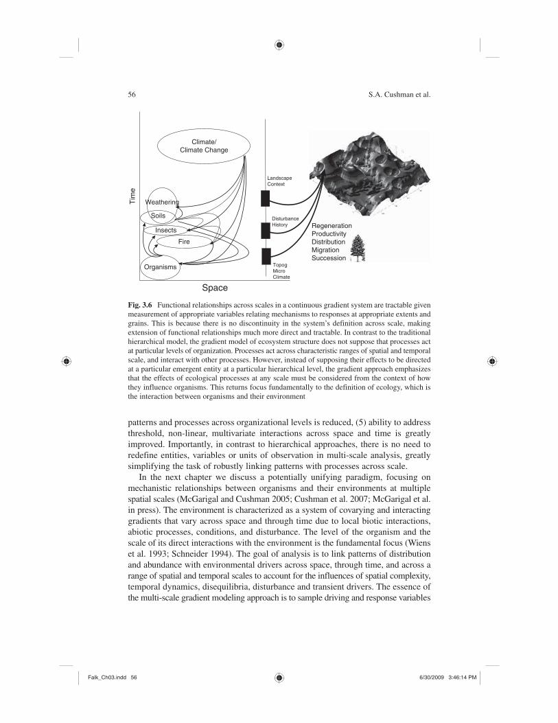
Linking mechanisms and responses across scale may benefit from approaches that use scalable rather than logical units. Multiscale analysis is facilitated by analysis in ratio scale units that can be expanded in extent, decimated in grain, and combined to make new units via multiplication and division (Schneider 1994, Fig. 3.6). Instead of focusing on efforts to estimate emergent properties of aggregate entities, it may be more fruitful to focus attention directly at the level of most biological interest, such as the organisms and its immediate interactions with the environment. Understanding relationships between mechanisms and ecological responses at that level may be facilitated by measuring relationships between organisms and their environment in ratio scale units at a fine grain and over broad extent. Such measure-ments of multiple parameters across space and through time form a gradient cube in which pattern–process relationships can be investigated simultaneously for a range of organisms and processes, and across a range of scales without the need to recode or reclassify the data (Cushman et al. in press).
Fig. 3.4 As an alternative to a hierarchical model of ecological system organization, with its attendant challenges of meaningfully defining entities across levels of organizations, and handling simultaneous change in scale and entity in analysis, we believe a gradient model is often more powerful, tractable and consistent with fundamental ecological theory than hierarchical models of system organization. Instead of inventing entities and struggling with the problem of defining them, their boundaries and characteristics, focus instead is on organisms and their interactions with fundamental driving factors across spatial and temporal scale. This removes one of the two major problems facing the traditional ecological organization: translation across entities. The second problem of translation across processes with scale is greatly facilitated. The relationship between processes and organism responses can be modeled continuously across scale. This provides a picture of how different processes interact and the nature of their influence as a function of scale
3 The Problem of Ecological Scaling in Spatially Complex 55
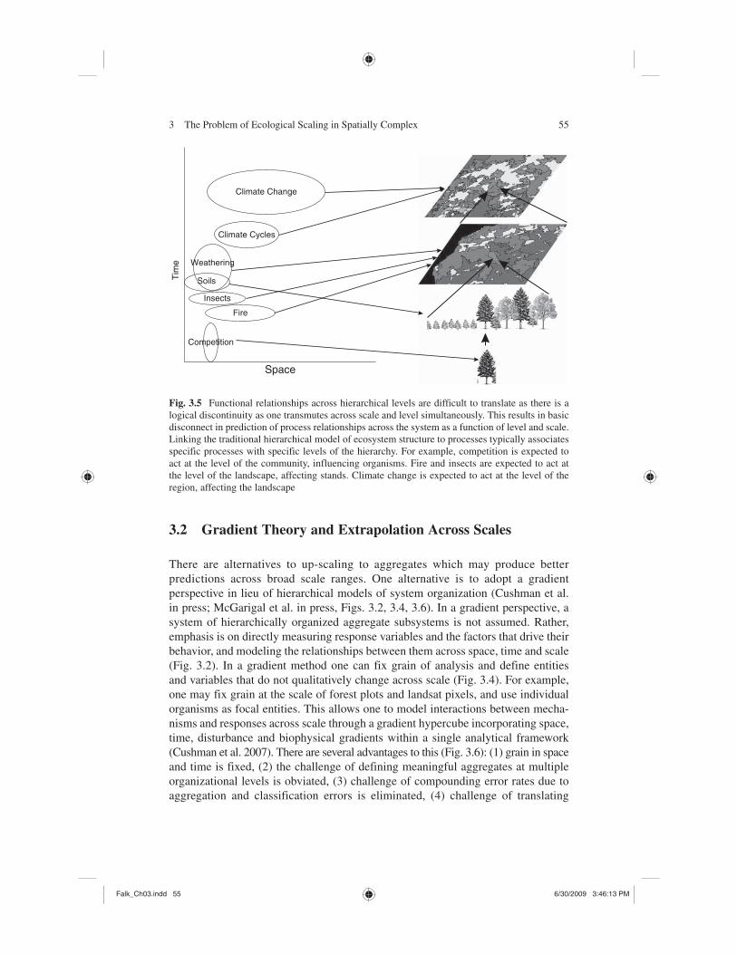
Fig. 3.5 Functional relationships across hierarchical levels are difficult to translate as there is a logical discontinuity as one transmutes across scale and level simultaneously. This results in basic disconnect in prediction of process relationships across the system as a function of level and scale. Linking the traditional hierarchical model of ecosystem structure to processes typically associates specific processes with specific levels of the hierarchy. For example, competition is expected to act at the level of the community, influencing organisms. Fire and insects are expected to act at the level of the landscape, affecting stands. Climate change is expected to act at the level of the region, affecting the landscape
Space
Climate Change
Climate Cycles
Fire
Insects
Competition
Soils
Weathering
Tim
e
3.2 Gradient Theory and Extrapolation Across Scales
There are alternatives to up-scaling to aggregates which may produce better predictions across broad scale ranges. One alternative is to adopt a gradient perspective in lieu of hierarchical models of system organization (Cushman et al. in press; McGarigal et al. in press, Figs. 3.2, 3.4, 3.6). In a gradient perspective, a system of hierarchically organized aggregate subsystems is not assumed. Rather, emphasis is on directly measuring response variables and the factors that drive their behavior, and modeling the relationships between them across space, time and scale (Fig. 3.2). In a gradient method one can fix grain of analysis and define entities and variables that do not qualitatively change across scale (Fig. 3.4). For example, one may fix grain at the scale of forest plots and landsat pixels, and use individual organisms as focal entities. This allows one to model interactions between mecha-nisms and responses across scale through a gradient hypercube incorporating space, time, disturbance and biophysical gradients within a single analytical framework (Cushman et al. 2007). There are several advantages to this (Fig. 3.6): (1) grain in space and time is fixed, (2) the challenge of defining meaningful aggregates at multiple organizational levels is obviated, (3) challenge of compounding error rates due to aggregation and classification errors is eliminated, (4) challenge of translating
patterns and processes across organizational levels is reduced, (5) ability to address threshold, non-linear, multivariate interactions across space and time is greatly improved. Importantly, in contrast to hierarchical approaches, there is no need to redefine entities, variables or units of observation in multi-scale analysis, greatly simplifying the task of robustly linking patterns with processes across scale.
In the next chapter we discuss a potentially unifying paradigm, focusing on mechanistic relationships between organisms and their environments at multiple spatial scales (McGarigal and Cushman 2005; Cushman et al. 2007; McGarigal et al. in press). The environment is characterized as a system of covarying and interacting gradients that vary across space and through time due to local biotic interactions, abiotic processes, conditions, and disturbance. The level of the organism and the scale of its direct interactions with the environment is the fundamental focus (Wiens et al. 1993; Schneider 1994). The goal of analysis is to link patterns of distribution and abundance with environmental drivers across space, through time, and across a range of spatial and temporal scales to account for the influences of spatial complexity, temporal dynamics, disequilibria, disturbance and transient drivers. The essence of the multi-scale gradient modeling approach is to sample driving and response variables
Fig. 3.6 Functional relationships across scales in a continuous gradient system are tractable given measurement of appropriate variables relating mechanisms to responses at appropriate extents and grains. This is because there is no discontinuity in the system’s definition across scale, making extension of functional relationships much more direct and tractable. In contrast to the traditional hierarchical model, the gradient model of ecosystem structure does not suppose that processes act at particular levels of organization. Processes act across characteristic ranges of spatial and temporal scale, and interact with other processes. However, instead of supposing their effects to be directed at a particular emergent entity at a particular hierarchical level, the gradient approach emphasizes that the effects of ecological processes at any scale must be considered from the context of how they influence organisms. This returns focus fundamentally to the definition of ecology, which is the interaction between organisms and their environment
3 The Problem of Ecological Scaling in Spatially Complex 57
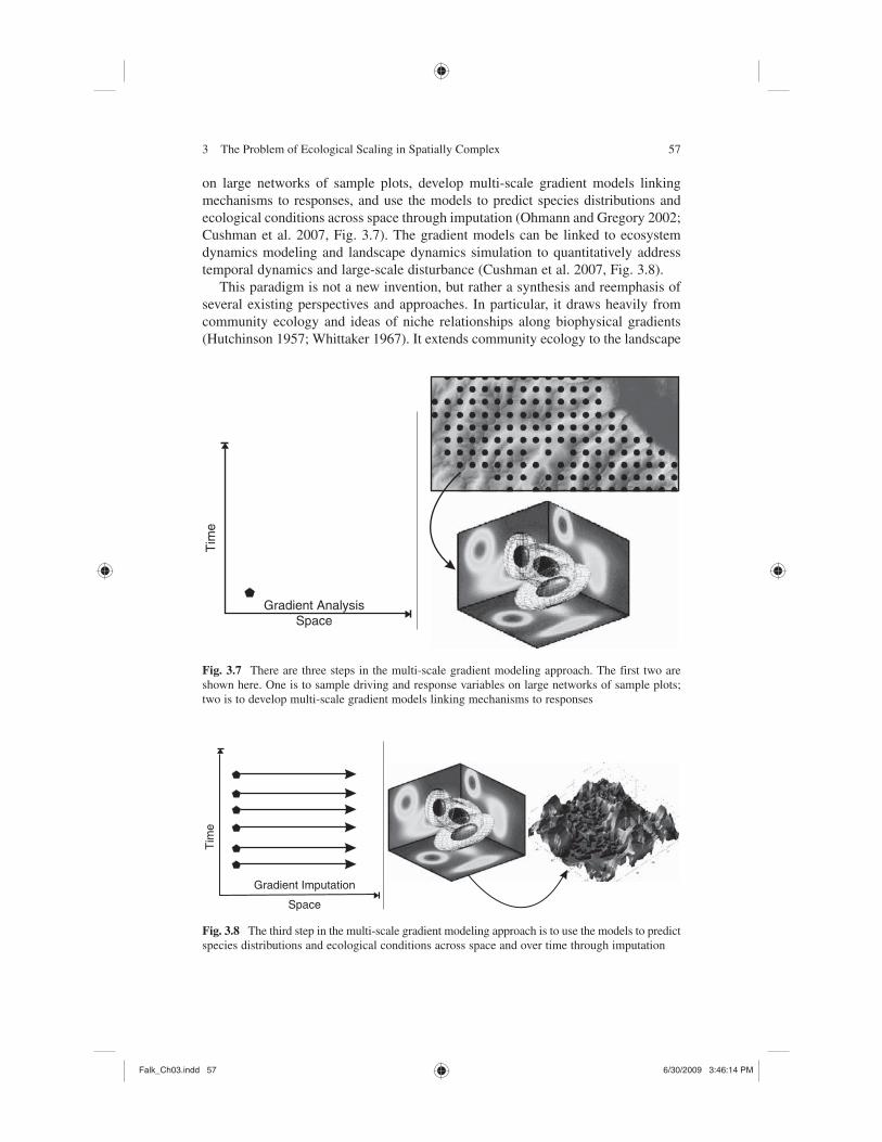
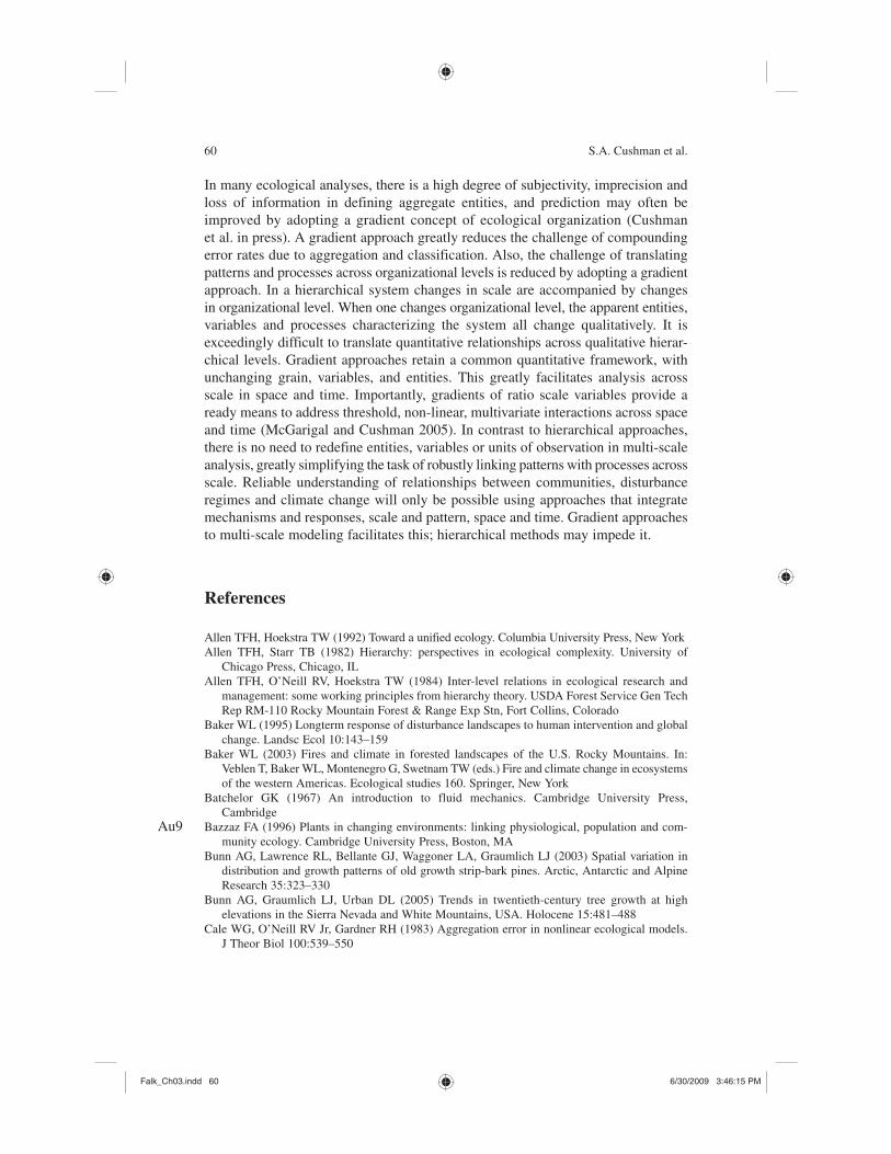
on large networks of sample plots, develop multi-scale gradient models linking mechanisms to responses, and use the models to predict species distributions and ecological conditions across space through imputation (Ohmann and Gregory 2002; Cushman et al. 2007, Fig. 3.7). The gradient models can be linked to ecosystem dynamics modeling and landscape dynamics simulation to quantitatively address temporal dynamics and large-scale disturbance (Cushman et al. 2007, Fig. 3.8).
This paradigm is not a new invention, but rather a synthesis and reemphasis of several existing perspectives and approaches. In particular, it draws heavily from community ecology and ideas of niche relationships along biophysical gradients (Hutchinson 1957; Whittaker 1967). It extends community ecology to the landscape
Fig. 3.7 There are three steps in the multi-scale gradient modeling approach. The first two are shown here. One is to sample driving and response variables on large networks of sample plots; two is to develop multi-scale gradient models linking mechanisms to responses
Gradient AnalysisSpace
Tim
e
Fig. 3.8 The third step in the multi-scale gradient modeling approach is to use the models to predict species distributions and ecological conditions across space and over time through imputation
level by explicitly addressing spatial complexity and temporal disequilibria, and by adopting a multi-scale approach. It extends landscape ecology by linking analysis of spatial and temporal patterns directly to organism responses to spatially and temporally varying environmental gradients. The traditional methods and theories of community and landscape ecology are different and have contributed to the long-standing disjunction between the fields. However, it is clear that a quantitative and conceptual synthesis between landscape and community ecology is essential if we are to address the key issues of how variation through space and time and across scale influence the relationships between organisms and their environments (Cushman et al. in press; McGarigal et al. in press). Schneider (1994) notes that rapid progress was made in meteorology and physical oceanography when fluid dynamics was taken out of pipes and put into a geophysical grid (Batchelor 1967; Pedlosky 1979) with attention to time and space scales (Stommel 1963). Similarly, the key to addressing spatially and temporally complex ecological systems is adopting a multi-scale, mechanistic paradigm. Linkage with geophysical gradient theory has been suggested as a means to accomplish this (Risser et al. 1988; Shugart et al. 1988; McGarigal et al. in press).
The approach incorporates aspects of a number of strategies suggested by other researchers. First, multivariate gradient modeling predicts all parameters simul-taneously, accounting for their covariation. As noted by Rastetter et al. (1992), simultaneous estimation of all parameters can substantially reduce propagated error (Hornberger and Cosby 1985). In addition it combines the principle of similitude and scope extrapolation suggested by Schneider (1994) with the method of extrapolation by increasing model extent discussed by King (1991). Extrapolation by increasing model extent uses a model for a single site to simulate the same processes for a collection of sites across the landscape. Each individual simulation requires data on the independent variables required by the fine-scale model. Thus, it is a case of using variables with large spatial scope to calculate a variable with a more limited scope (Schneider 1994). As King (1991) notes, model structure is unaltered, grain is not changed and there is no averaging or aggregating of the data.
In the principle of similitude, spatial or temporal variation in a variable is expressed as a function of location or time (Schneider 1994). Dimensionless ratios are formed and these are used to scale measurements of limited scope to expected values at larger scope. Due to the spatial complexity of the physical environment and the typically low correlation between spatial and environmental gradients the principle of similitude would seem to have limited direct application to predicting ecological phenomena across complex landscapes. However, gradient imputation can be considered a method of similitude in environmental space rather than geographical space. Multi-scale gradient models predict species responses as functions of continuously varying environmental gradients. The gradient space depicted in the models is continuous in n-dimensions without break or deviation in rate of change. Gradient modeling involves predicting response variables across space for locations where they have not been sampled based on where those locations occur in environ-mental gradient space, and what the expected value of the response variable is at that location in gradient space. The connection to similitude is that variation as a
3 The Problem of Ecological Scaling in Spatially Complex 59
function of location in ‘gradient space’ is used to develop scaling ratios for inferring values not sampled from values sampled.
3.3 Summary and Conclusions
Ecological processes are difficult to predict at the landscape level. Inconsistency of concepts, sampling, and analytical approaches across scales and organizational levels make it difficult to extend knowledge up the ecological hierarchy from plots and stands to landscapes, or down the hierarchy from biomes and regions to land-scapes. Moving down the organizational hierarchy from continents and regions to landscapes, broad scale relationships between regional climate and regional productivity and other forest parameters become unstable. As you move downward to landscapes, the details of the spatial structure of the landscape in terms of topography and soils becomes critical, as do historical events such as disturbance and temporal processes such as succession. Simultaneously, it is logistically and analytically difficult to extend fine-scale mechanistic relationships between individual organisms and their environments across space and time. Thus researchers face the challenging task of linking relationships across levels of organization, and translating between measurements and relationships of different entities at different scales. This simul-taneous challenge of translating among scales and organizational levels is the fundamental challenge to reliable prediction of forest ecosystems across spatial and temporal scale. There are at least four important parts of this challenge. First is a problem of transfer and deals with scale mismatches between drivers and responses. Second is a problem of heterogeneity and deals with spatial patterns of vegetation and the environment. Third is stationarity and deals with the transience in the drivers. Fourth is a problem of extrapolation that results from nested gradients interacting across scales in space and time. Understanding and predicting the responses of forest resources to changing climate and disturbance regimes requires approaches that link mechanisms to responses across scales while accounting for spatial and temporal variability.
The dominant paradigm that has guided most research in this arena is the hierarchical model of ecological systems (Allen and Starr 1982; O’Neil et al. 1986). In this model, ecological systems are conceptualized as nested collections of aggregate subsystems. Each subsystem is contains qualitatively different entities than those existing above and below, and is subject to influences of processes acting at different spatial and temporal scales (O’Neil et al. 1986). Levels of organization in a nested hierarchy occur within monotonically increasing scales of time and space, with lower levels characterized by smaller finer scales and finer temporal scales (King 1991). Urban et al. (1987) defined one such nested hierarchy for forest systems consisting of gaps, stands, watersheds and landscapes.
However, the hierarchical model faces a number of challenges, particularly in its ability to address interacting processes across a range of scales. First is the challenge of defining meaningful aggregates at multiple organizational levels (Schneider 1994).
In many ecological analyses, there is a high degree of subjectivity, imprecision and loss of information in defining aggregate entities, and prediction may often be improved by adopting a gradient concept of ecological organization (Cushman et al. in press). A gradient approach greatly reduces the challenge of compounding error rates due to aggregation and classification. Also, the challenge of translating patterns and processes across organizational levels is reduced by adopting a gradient approach. In a hierarchical system changes in scale are accompanied by changes in organizational level. When one changes organizational level, the apparent entities, variables and processes characterizing the system all change qualitatively. It is exceedingly difficult to translate quantitative relationships across qualitative hierar-chical levels. Gradient approaches retain a common quantitative framework, with unchanging grain, variables, and entities. This greatly facilitates analysis across scale in space and time. Importantly, gradients of ratio scale variables provide a ready means to address threshold, non-linear, multivariate interactions across space and time (McGarigal and Cushman 2005). In contrast to hierarchical approaches, there is no need to redefine entities, variables or units of observation in multi-scale analysis, greatly simplifying the task of robustly linking patterns with processes across scale. Reliable understanding of relationships between communities, disturbance regimes and climate change will only be possible using approaches that integrate mechanisms and responses, scale and pattern, space and time. Gradient approaches to multi-scale modeling facilitates this; hierarchical methods may impede it.
References
Allen TFH, Hoekstra TW (1992) Toward a unified ecology. Columbia University Press, New YorkAllen TFH, Starr TB (1982) Hierarchy: perspectives in ecological complexity. University of
Chicago Press, Chicago, ILAllen TFH, O’Neill RV, Hoekstra TW (1984) Inter-level relations in ecological research and
management: some working principles from hierarchy theory. USDA Forest Service Gen Tech Rep RM-110 Rocky Mountain Forest & Range Exp Stn, Fort Collins, Colorado
Baker WL (1995) Longterm response of disturbance landscapes to human intervention and global change. Landsc Ecol 10:143–159
Baker WL (2003) Fires and climate in forested landscapes of the U.S. Rocky Mountains. In: Veblen T, Baker WL, Montenegro G, Swetnam TW (eds.) Fire and climate change in ecosystems of the western Americas. Ecological studies 160. Springer, New York
Batchelor GK (1967) An introduction to fluid mechanics. Cambridge University Press, Cambridge
Bazzaz FA (1996) Plants in changing environments: linking physiological, population and com-munity ecology. Cambridge University Press, Boston, MA
Bunn AG, Lawrence RL, Bellante GJ, Waggoner LA, Graumlich LJ (2003) Spatial variation in distribution and growth patterns of old growth strip-bark pines. Arctic, Antarctic and Alpine Research 35:323–330
Bunn AG, Graumlich LJ, Urban DL (2005) Trends in twentieth-century tree growth at high elevations in the Sierra Nevada and White Mountains, USA. Holocene 15:481–488
Cale WG, O’Neill RV Jr, Gardner RH (1983) Aggregation error in nonlinear ecological models. J Theor Biol 100:539–550
3 The Problem of Ecological Scaling in Spatially Complex 61
Chesson PL (1981) Models for spatially distributed populations: the effect of within-patch variability. Theor Popul Biol 19:288–325
Clark JS (1990) Integration of ecological levels: individual plant growth, population mortality, and ecosystem dynamics. J Ecol 78:275–299
Collins SL, Knapp AK, Briggs JM, Blair JM, Steinhauer EM (1998) Modulation of diversity by grazing and mowing in native tallgrass prairie. Science 280:745–747
Cushman SA, McGarigal K (2003) Hierarchical, multi-scale decomposition of species-environment relationships. Landsc Ecol 17:637–646
Cushman SA, McKenzie D, Peterson DL, Littell J, McKelvey KS (2007) Research agenda for integrated landscape modelling. USDA For Serv Gen Tech Rep RMRS-GTR-194
Cushman SA, Evans J, McGarigal K (in press) Do classified vegetation maps predict the composition of plant communities? The need for Gleasonian landscape ecology. Landsc Ecol
Dunwiddie PW (1986) A 6000-year record of forest history on Mount Rainier, Washington. Ecology 67:58–68
Finegan B (1984) Forest succession. Nature 312:109–114Gardner RH, Cale WG, O’Neill RV (1982) Robust analysis of aggregation error. Ecology
63:1771–1779Gates WL (1985) The use of general circulation models in the analysis of the ecosystem impacts
of climatic change. Climatic Change 7:267–284Glenn SM, Collins SL (1992) Disturbances in tallgrass prairie—local and regional effects on
community heterogeneity. Landsc Ecol 7:243–251Hornberger GM, Cosby BJ (1985) Evaluation of a model of long-term response of catchments to
atmospheric deposition of sulfate. In: Proceedings of the 7th IFAC symposium on identification and system parameter estimation. Pergamon, New York
Hutchinson GE (1957) Concluding remarks. Cold Spring Harbor Symp Quant Biol 22:414–427Iwasa Y, Andreasen V, Levin S (1987) Aggregation in model ecosystems: I. perfect aggregation.
Ecoll Model 37:287–302Iwasa Y, Levin S, Andreasen V (1989) Aggregation in model ecosystems: II. approximate aggre-
gation. IMA J Math Appl Med Biol 6:1–23Jeffers JNR (1988) Statistical and mathematical approaches to issues of scale in ecology. In:
Rosswall TR, Woodmansee RG, Risser, PG (eds) Scale and global changes: spatial and temporal variability in biospheric and geospheric process. Wiley, Chichester
Kareiva P, Andersen M (1986) Spatial aspects of species interactions: the wedding of models and experiments. In: Hastings A (ed) Community ecology: lecture notes in biomathematics. Springer, Berlin
Kareiva PM (1994) Space: the final frontier for ecological theory. Ecology 75:1Kennedy AD (1997) Bridging the gap between general circulation model (GCM) output and
biological microenvironments. Int J Biometeorol 40:119–122King AW (1991) Translating models across scales in the landscape. In: Turner MG, Gardner RH
(eds) Quantitative methods in landscape ecology, ecological studies, vol 82. Springer, New YorkLevin SA (1992) The problem of pattern and scale in ecology. Ecology 73:1943–1967Lynn BH, Rind D, Avissar A (1995) The importance of mesoscale circulations generated by
subgrid-scale landscape heterogeneities in general-circulation models. J Clim 8:191–205McGarigal K, Cushman SA (2002) Comparative evaluation of experimental approaches to the
study of habitat fragmentation effects. Ecol Appl 12:335–345McGarigal K, Cushman SA (2005) The gradient concept of landscape structure. In: Wiens JA,
Moss MR (eds) Issues and perspectives in landscape ecology. Cambridge University Press, Cambridge
McGariga l K, Tagil S, Cushman SA (in press) Surface metrics: an alternative to patch metrics for the quantification of landscape structure. Landsc Ecol
Meetenmeyer V, Box EO (1987) Scale effects in landscape studies. In: Turner, MG (ed) Landscape heterogeneity and disturbance. Springer, New York
Mooney HA, Godron M (1983) Disturbance and ecosystems. Springer, New York
Ohmann JL, Gregory MJ (2002) Predictive mapping of forest composition and structure with direct gradient analysis and nearest-neighbor imputation in coastal Oregon, USA. Can J Forest Resources 32:725–741
O’Neill RV (1979) Transmutations across hierarchical levels. In: Innis SG, O’Neill RV (eds) Systems analysis of ecosystems. International Cooperative Publishing House, Fairland
O’Neill RV (1988) Perspectives in hierarchy and scale. In: Roughgarden J, May RM, Levin, SA (eds) Perspectives in ecological theory. Princeton University Press, Princeton, NJ
O’Neill RV, DeAngelis DL,Waide JB, Allen, TFH (1986) A hierarchical concept of ecosystems. Princeton University Press, Princeton, NJ
Patten BC (1982) Environs: relativistic elementary particles for ecology. Am N 119:179–219.Pedlosky J (1979) Geophysical fluid dynamics. Springer, New YorkPeet SK, Loucks OL (1976) A gradient analysis of southern Wisconsin forests. Ecology 58:485–499Peterson DL, Parker VT (1998) Ecological scale: theory and applications. Columbia University
Press, New YorkPickett STA (1980) Non-equilibrium coexistence of plants. Bull Torrey Bot Club 107:238–248Rastetter EB, King AW, Cosby BJ, Hornberger GM, O’Neill RV, Hobbie JE (1992) Aggregating
fine-scale ecological knowledge to model coarser-resolution attributes of ecosystems. Ecol Applic 2:55–70
Reynolds JF, Hilbert DW, Kemp PW (1993) Scaling ecophysiology from the plant to the ecosystem: a conceptual framework. In: Ehleringer JR, Field CB (eds) Scaling physiological processes. Academic Press, New York
Risser PG (1986) Report of a workshop on the spatial and temporal variability of biospheric and geospheric processes: research needed to determine interactions with global environmental change, Oct. 28-Nov.1, 1985. St. Petersburg, Fla. Paris: ICSU Press.
Risser PG (1987) Landsacpe ecology: state of the art. In: Turner, MG (ed) Landscape heterogeneity and disturbance. Springer, New York
Risser PG, Karr JR, Forman RTT (1984) Landscape ecology: directions and approaches. Special Publication Number 2. Illinois Natural History Survey, Champaign
Roswall T, Woodmansee RG, Risser PG (eds) Scales in global change. Wiley, New York, 1988? Spelling?
Runkle JR (1985) Disturbance regimes in temperate forests. In S.T.A. Pickett and P.S. White, eds. The ecology of natural disturbance and patch dynamics, pp. 17–34, Academic, New York
Russo JM, Zack JW (1997) Downscaling GCM output with a mesoscale model. J Environ Manag 49:19–29.
Schneider DC (1994) Quantitative ecology: spatial and temporal scaling. Academic, San Diego, CAShugart HH, Urban DL (1988) Scale, synthesis, and ecosystem dynamics. In: Pomeroy LR,
Alberts JJ (eds) Concepts of ecosystem ecology. Springer, New YorkShugart HH, Michaels PJ, Smith TM, Weinstein DA, Rastetter EB (1988) Simulation models of
forest succession. In: Roswall T, Woodmansee RG, Risser PG (eds) Scales in global change. Wiley, New York
Sousa WP (1984) The role of disturbance in natural communities. Annul Rev Ecol Systemat 15:353–391
Stommel H (1963) The varieties of oceanographic experience. Science 139:572–576ter Braak CJF, Prentice IC (1988) A theory of gradient analysis. Adv Ecol Res 18:271–313.Tilman D (1982) Resource competition and community structure. Princeton University Press,
Princeton, NJTurner MG (1989) Landscape ecology: the effect of pattern on process. Annu Rev Ecol Systemat
20:171–197Turner MG, Dale VH (1998) Comparing large, infrequent disturbances: what have we learned?
Introduction for special feature. Ecosystems 1:493–496Turner MG, Gardner RH, O’Neill RV (2001) Landscape ecology in theory and practice. Springer,
New YorkUrban DL, O’Neill RV, Shugart HH Jr (1987) Landscape ecology. Bioscience 37:119–27.Watt AS (1947) Pattern and process in the plant community. J Ecol 35:1–22
3 The Problem of Ecological Scaling in Spatially Complex 63
Wagner HM (1969) Principles of operations research. Prentice-Hall, Englewood Cliffs, NJ.Webster JR (1979) Hierarchical organization of ecosystems. In: Halfon E (ed) Theoretical systems
ecology. Academic, New YorkWelsh AH, Peterson TA, Altmann SA (1988) The fallacy of averages. Am Nat 132:277–288.White PS (1979) Pattern, process, and natural disturbance in vegetation. Bot Rev 45:229–299Whittaker RH (1967). Gradient analysis of vegetation. Biol Rev 49:207–264Wiens JA (1989) Spatial scaling in ecology. Funct Ecol 3:385–397.Wiens JA, Stenseth NC, Van Horne B, Ims RA (1993) Ecological mechanisms and landscape