191
The Quicksort algorithm and related topics Vasileios Iliopoulos A thesis submitted for the degree of Doctor of Philosophy Department of Mathematical Sciences University of Essex June 2013

The Quicksort algorithmand related topics
Vasileios Iliopoulos
A thesis submitted for the degree ofDoctor of Philosophy
Department of Mathematical SciencesUniversity of Essex
June 2013


Abstract
Sorting algorithms have attracted a great deal of attention and study, as they
have numerous applications to Mathematics, Computer Science and related
fields. In this thesis, we first deal with the mathematical analysis of the Quick-
sort algorithm and its variants. Specifically, we study the time complexity of
the algorithm and we provide a complete demonstration of the variance of the
number of comparisons required, a known result but one whose detailed proof
is not easy to read out of the literature. We also examine variants of Quicksort,
where multiple pivots are chosen for the partitioning of the array.
The rest of this work is dedicated to the analysis of finding the true order by
further pairwise comparisons when a partial order compatible with the true
order is given in advance. We discuss a number of cases where the partially
ordered sets arise at random. To this end, we employ results from Graph and
Information Theory. Finally, we obtain an alternative bound on the number of
linear extensions when the partially ordered set arises from a random graph,
and discuss the possible application of Shellsort in merging chains.
iii


Acknowledgements
I would like to thank Dr. David B. Penman for his meticulous advise and guid-
ance, as I pursued this work. Our fruitful conversations helped me to clearly
express my ideas in this thesis. Thanks are also due to Dr. Gerald Williams for
his comments and suggestions during board meetings.
I dedicate this work to my family. Without their support, I wouldn’t be able to
carry out and accomplish my research.
v
Contents
1 Preface 1
1.1 Preliminaries . . . . . . . . . . . . . . . . . . . . . . . . . . . . 1
1.2 Definitions . . . . . . . . . . . . . . . . . . . . . . . . . . . . . . 3
1.3 Introduction to Quicksort . . . . . . . . . . . . . . . . . . . . . 5
1.4 Outline and contributions of thesis . . . . . . . . . . . . . . . . 10
2 Random selection of pivot 13
2.1 Expected number of comparisons . . . . . . . . . . . . . . . . . 13
2.2 Expected number of exchanges . . . . . . . . . . . . . . . . . . 21
2.3 Variance . . . . . . . . . . . . . . . . . . . . . . . . . . . . . . . 24
2.4 “Divide and Conquer” recurrences . . . . . . . . . . . . . . . . . 38
2.5 Higher moments . . . . . . . . . . . . . . . . . . . . . . . . . . 42
2.6 Asymptotic analysis . . . . . . . . . . . . . . . . . . . . . . . . . 45
2.6.1 Binary trees . . . . . . . . . . . . . . . . . . . . . . . . . 46
2.6.2 Limiting behaviour . . . . . . . . . . . . . . . . . . . . . 49
2.6.3 Deviations of Quicksort . . . . . . . . . . . . . . . . . . 58
2.7 Quicksorting arrays with repeated elements . . . . . . . . . . . 62
3 Sorting by sampling 64
3.1 Median of (2k+1) partitioning . . . . . . . . . . . . . . . . . . 65
3.2 Remedian Quicksort . . . . . . . . . . . . . . . . . . . . . . . . 78
vi
3.3 Samplesort . . . . . . . . . . . . . . . . . . . . . . . . . . . . . 81
4 Sorting by multiple pivots 85
4.1 Quicksorting on two pivots . . . . . . . . . . . . . . . . . . . . . 86
4.1.1 The variance of the number of key comparisons . . . . . 95
4.1.2 Distribution of the number of key comparisons . . . . . 99
4.2 Multikey partitioning . . . . . . . . . . . . . . . . . . . . . . . . 102
4.2.1 Derivation of integration constants using Vandermonde
matrices . . . . . . . . . . . . . . . . . . . . . . . . . . . 114
4.3 Multipivot–median partitioning . . . . . . . . . . . . . . . . . . 118
5 Partial order of keys 123
5.1 Introduction . . . . . . . . . . . . . . . . . . . . . . . . . . . . . 123
5.2 Partially ordered sets . . . . . . . . . . . . . . . . . . . . . . . . 125
5.3 Uniform random partial orders . . . . . . . . . . . . . . . . . . 132
5.4 Random bipartite orders . . . . . . . . . . . . . . . . . . . . . . 136
5.5 Random k–dimensional orders . . . . . . . . . . . . . . . . . . 138
5.6 Random interval orders . . . . . . . . . . . . . . . . . . . . . . 141
6 Linear extensions of random graph orders 148
6.1 Random graph orders . . . . . . . . . . . . . . . . . . . . . . . 148
6.2 Additive parameters and decomposing posets . . . . . . . . . . 152
6.3 Average height of random graph orders . . . . . . . . . . . . . . 155
6.4 Bounds on the height of random graph orders . . . . . . . . . . 161
6.5 Expected number of linear extensions . . . . . . . . . . . . . . . 164
7 Conclusions and future research directions 167
7.1 Sorting partially ordered arrays . . . . . . . . . . . . . . . . . . 167
vii
7.2 Merging chains using Shellsort . . . . . . . . . . . . . . . . . . 169
Appendix A MAPLE Computations 173
Bibliography 176
viii

Chapter 1
Preface
The first Chapter serves as an introduction to this work, where in a simple man-
ner, useful notions of algorithmic analysis in general are presented, along with
definitions that will be used throughout the thesis. We present an introduction
to Quicksort and this Chapter ends with an outline and a summary of the main
contributions of this thesis.
1.1 Preliminaries
An algorithm is a valuable tool for solving computational problems. It is a
well defined procedure that takes some value or a set of values as input and
is guaranteed to produce an answer in finite time. See e.g. [15]. However the
time taken may be impractically long.
As a useful introduction, we present a simple and intuitive algorithm known as
Euclid’s algorithm which is still used today to determine the greatest common
divisor of two integers. Its definition follows [45]:
Definition 1.1.1. Given two integers A ≥ C greater than unity, we want to find
their greatest common divisor, g.c.d.(A, C).
1
2
1. If C divides A, then the algorithm terminates with C as the greatest common
divisor.
2. If A mod C is equal to unity, the numbers are either prime or relatively
prime and the algorithm terminates. Otherwise set A← C, C ← A mod C
and return to step 1.
By A mod C, we denote the remainder of the division of A by C, namely
A mod C := A−(C ·⌊A
C
⌋),
which is between 0 and C − 1. Here the floor function bxc of a real number x
is the largest integer less than or equal to x. We observe that this algorithm
operates recursively by successive divisions, until obtaining remainder equal
to 0 or to 1. Since the remainder strictly reduces at each stage, the process is
finite and eventually terminates.
Two main issues in relation to an algorithm are its running time or time com-
plexity, which is the amount of time necessary to solve the problem, and its
space complexity, which is the amount of memory needed for the execution
of the algorithm in a computer. In case of Euclid’s algorithm, 3 locations of
memory are required for storing the integer numbers A, C and A mod C. In
this thesis, we will mainly be concerned with time complexity.
The aim is usually to relate the time complexity to some measure of the size of
the instance of the problem we are considering. Very often we are particularly
concerned with what happens when the size n is large – tending to infinity. The
notations O, Ω, Θ and o, ω are useful in this context.
3
1.2 Definitions
In this section, we present primary definitions to the analysis presented in the
thesis. These definitions come from [15], [26].
Definition 1.2.1. Let f(n) and g(n) be two functions with n ∈ N. We say that
f(n) = O(g(n)
)if and only if there exists a constant c > 0 and n0 ∈ N, such that
|f(n)| ≤ c · |g(n)|, ∀n ≥ n0.
Definition 1.2.2. Also, we say that f(n) = Ω(g(n)
)if and only if there exists a
constant c > 0 and n0 ∈ N, such that |f(n)| ≥ c · |g(n)|, ∀n ≥ n0.
Definition 1.2.3. Furthermore, we say that f(n) = Θ(g(n)
)if and only if there
exist positive constants c1, c2 and n0 ∈ N, such that c1 ·|g(n)| ≤ |f(n)| ≤ c2 ·|g(n)|,
∀n ≥ n0. Equivalently, we can state that if f(n) = O(g(n)
)and f(n) = Ω
(g(n)
),
then f(n) = Θ(g(n)
).
We will also use the notations o, ω. They provide the same kind of limiting
bounds with the respective upper case notations. The difference is that for
two functions f(n) and g(n), the upper case notation holds when it does exist
some positive constant c. Whereas, the respective lower case notation is true
for every positive constant c [15]. In other words, o is stronger statement than
O, since f(n) = o(g(n)
)implies that f is dominated by g. Equivalently, this can
be stated as
f(n) = o(g(n)
)⇐⇒ lim
n→∞
f(n)
g(n)= 0,
provided that g(n) is non-zero.
4
The relation f(n) = ω(g(n)
)implies that f dominates g, i.e.
f(n) = ω(g(n)
)⇐⇒ lim
n→∞
f(n)
g(n)=∞.
The relation f(n) ∼ g(n) denotes the fact that f(n) and g(n) are asymptotically
equivalent, i.e.
limn→∞
f(n)
g(n)= 1.
Further, best, worst and average case performance denote the resource usage,
e.g. amount of memory in computer or running time, of a given algorithm at
least, at most and on average, respectively. In other words, these terms describe
the behaviour of an algorithm under optimal circumstances (e.g. best–case
scenario), worst circumstances and on average [15]. In this work, the study
will be concentrated on the average and worst case performance of Quicksort
and its variants.
In our analysis, we will frequently come across with harmonic numbers, whose
definition we now present.
Definition 1.2.4. The sum
H(k)n :=
n∑i=1
1
ik=
1
1k+
1
2k+ . . .+
1
nk
is defined to be the generalised nth harmonic number of order k. When k = 1, the
sum denotes the nth harmonic number, which we simply write Hn. We define also
H0 := 0.
There are numerous interesting properties of harmonic numbers, which are not
yet fully investigated and understood. Harmonic series have links with Stirling
5
numbers [26] and arise frequently in the analysis of algorithms. For n large, it
is well-known that [44],
Hn = loge(n) + γ +1
2n− 1
12n2+
1
120n4+O
(1
n6
),
where γ = 0.57721 . . . is the Euler–Mascheroni constant. We will use this often,
especially in the form Hn = loge(n) + γ + o(1).
Note that throughout this thesis, we shall adopt the convention of writing
explicitly the base of logarithms. For example, the natural logarithm of n is
denoted by loge(n), instead of ln(n). Also, the end of a proof will be denoted
by the symbol .
1.3 Introduction to Quicksort
Sorting an array of items is clearly a fundamental problem, directly linked
to efficient searching with numerous applications. The problem is that given
an array of keys, we want to rearrange these in non-decreasing order. Note
that the order may be numerical, alphabetical or any other transitive relation
defined on the keys [46]. In this work, the analysis deals with numerical order,
where the keys are decimal numbers and we particularly focus on Quicksort
algorithm and variants of it. Quicksort was invented by C. A. R. Hoare [29, 30].
Here is the detailed definition.
Definition 1.3.1.
The steps taken by the Quicksort algorithm are:
1. Choose an element from the array, called pivot.

6
2. Rearrange the array by comparing every element to the pivot, so all elements
smaller than or equal to the pivot come before the pivot and all elements
greater than or equal to the pivot come after the pivot.
3. Recursively apply steps 1 and 2 to the subarray of the elements smaller than
or equal to the pivot and to the subarray of the elements greater than or
equal to the pivot.
Note that the original problem is divided into smaller ones, with (initially)
two subarrays, the keys smaller than the pivot, and those bigger than it. Then
recursively these are divided into smaller subarrays by further pivoting, until we
get trivially sorted subarrays, which contain one or no elements. Given an array
of n distinct keys A = a1, a2, . . . , an that we want to quick sort, with all the
n! permutations equally likely, the aim is to finding the unique permutation out
of all the n! possible, such that the keys are in increasing order. The essence of
Quicksort is the partition operation, where by a series of pairwise comparisons,
the pivot is brought to its final place, with smaller elements on its left and
greater elements to the right. Elements equal to pivot can be on either or both
sides.
As we shall see, there are numerous partitioning schemes, and while the details
of them are not central to this thesis, we should describe the basic ideas. A
straightforward and natural way (see e.g. [46]) uses two pointers – a left
pointer, initially at the left end of the array and a right pointer, initially at the
right end of the array. We pick the leftmost element of the array as pivot and
the right pointer scans from the right end of the array for a key less than the
pivot. If it finds such a key, the pivot is swapped with that key. Then, the left
pointer is increased by one and starts its scan, searching for a key greater than
7
the pivot: if such a key is found, again the pivot is exchanged with it. When
the pointers are crossed, the pivot by repeated exchanges will “float” to its final
position and the keys which are on its left are smaller and keys on its right
are greater. The data movement of this scheme is quite large, since the pivot is
swapped with the other elements.
A different partitioning scheme, described in [30] is the following. Two pointers
i (the left pointer, initially 1) and j (the right pointer, initially n) are set and a
key is arbitrarily chosen as pivot. The left pointer goes to the right until a key
is found which is greater than the pivot. If one is found, its scan is stopped and
the right pointer scans to the left until a key less than the pivot is found. If such
a key is found, the right pointer stops and those two keys are exchanged. After
the exchange, both pointers are stepped down one position and the lower one
starts its scan. When pointers are crossed, i.e. when i ≥ j, the final exchange
places the pivot in its final position, completing the partitioning. The number
of comparisons required to partition an array of n keys is at least n− 1 and the
expected number of exchanges is n6
+ 56n
.
A third partitioning routine, called Lomuto’s partition, is mentioned in [6] –
this involves exactly n− 1 comparisons, which is clearly best possible, but the
downside is the increased number of exchanges. The expected number of key
exchanges of this scheme is n−12
, [48].
We now consider the worst case and best case, analysis of Quicksort. Suppose
we want to sort the following array, a1 < a2 < . . . < an and we are very
unlucky and our initial choice of pivot is the largest element an. Then of course
we only divide and conquer in a rather trivial sense: every element is below the
pivot, and it has taken us n− 1 comparisons with an to get here. Suppose we
8
now try again and are unlucky again, choosing an−1 as pivot this time. Again
the algorithm performs n− 2 comparisons and we are left with everything less
than an−1. If we keep being unlucky in our choices of pivot, and keep choosing
the largest element of what is left, after i recursive calls the running time of
the algorithm will be equal to (n− 1) + (n− 2) + . . .+ (n− i) comparisons, so
the overall number of comparisons made is
1 + 2 + . . .+ (n− 1) =n · (n− 1)
2.
Thus Quicksort needs quadratic time to sort already sorted or reverse-sorted
arrays if the choice of pivots is unfortunate.
If instead we always made good choices, choosing each pivot to be roughly in
the middle of the array we are considering at present, then in the first round
we make n − 1 comparisons, then in the two subarrays of size about n/2 we
make about n/2 comparisons, then in each of the four subarrays of size about
n/4 we make n/4 comparisons, and so on. So we make about n comparisons
in total in each round. The number of rounds will be roughly log2(n) as we are
splitting the arrays into roughly equally-sized subarrays at each stage, and it
will take log2(n) recursions of this to get down to trivially sorted arrays.
Thus, in this good case we will needO(n log2(n)
)comparisons. This is of course
a rather informal argument, but does illustrate that the time complexity can
be much smaller than the quadratic run-time in the worst case. This is already
raising the question of what the typical time complexity will be: we address
this in the next Chapter.
9
We briefly discuss the space complexity of the algorithm. There are n memory
locations occupied by the keys. Moreover, the algorithm, due to its recursive
nature, needs additional space for the storage of subarrays. The subarrays’
boundaries are saved on to a stack, which is a data structure providing tempo-
rary storage. At the end of the partition routine, the pivot is placed in its final
position between two subarrays (one of them possibly empty). Recursively, the
algorithm is applied to the smaller subarray and the other one is pushed on to
stack. Since, in best and average case of Quicksort, we have O(log2(n)
)recur-
sive calls, the required stack space is O(log2(n)
)locations in memory. However,
in worst case the stack may require O(n) locations, if the algorithm is applied
to the larger subarray and the smaller one is saved to the stack [63].
This discussion makes it clear that the pivot selection plays a vital role in the
performance of the algorithm. Many authors have proposed various techniques
to remedy this situation and to avoid worst case behaviour, see [15], [30], [46],
[62], [63] and [68]. These include the random shuffling of the array prior to
initialisation of the algorithm, choosing as pivot the median of the array, or the
median of a random sample of keys.
Scowen in his paper [62], suggested choosing as pivot the middle element of
the array: his variant is dubbed “Quickersort”. Using this rule for the choice
of partitioning element, the aim is the splitting of the array into two halves
of equal size. Thus, in case where the array is nearly sorted, quadratic time is
avoided but if the chosen pivot is the minimum or maximum key, the algorithm’s
running time attains its worst case and this variant does not offer any more
than choosing the pivot randomly. Singleton [68] suggested a better estimate of
the median, by selecting as pivot the median of leftmost, rightmost and middle
10
keys of the input array. Hoare [30] suggested the pivot may be chosen as the
median of a random sample from the keys to be sorted, but he didn’t analyse
this approach.
One point is that Quicksort is not always very fast at sorting small arrays. Knuth
[46] presented and analysed a partitioning scheme, which takes n+1 instead of
n− 1 comparisons and the sorting of small subarrays (usually from about 9 to
15 elements) is implemented using insertion sort, since the recursive structure
of Quicksort is better suited to large arrays. Insertion sort is a simple sorting
algorithm, which gradually ‘constructs’ a sorted array from left to right, in the
following manner. The first two elements are compared and exchanged, in case
that are not in order. Then, the third element is compared with the element on
its left. If it is greater, it is left at its initial location, otherwise is compared with
the first element and accordingly is inserted to its position in the sorted array
of 3 elements. This process is iteratively applied to the remaining elements,
until the array is sorted. See as well in Cormen et al. [15], for a description of
the algorithm.
1.4 Outline and contributions of thesis
This thesis consists of seven Chapters and one Appendix. After the first, intro-
ductory Chapter, the rest of the thesis is organised as follows:
In Chapter 2, we consider the first and second moments of the number of
comparisons made when pivots are chosen randomly. The result for the mean
is known and easy: the result for the variance is known, but less easy to find a
full proof of in the literature. We supply one. We briefly discuss the skewness
11
of the number of comparisons and we study the asymptotic behaviour of the
algorithm.
In Chapter 3, we analyse the idea of choosing the pivot as a centered statistic
of a random sample of the keys to be sorted and we obtain the average number
of comparisons required by these variants, showing that the running time can
be greatly improved. Moreover, we present relevant definitions of entropy. Not
much of this is original, but some details about why various differential equa-
tions that arise in the analysis have the solutions they do (i.e. details about
roots of indicial polynomials) are not in literature.
In Chapter 4, we analyse extensions of Quicksort, where multiple pivots are
used for the partitioning of the array. The main contributions in this Chapter
are in sections 4.1 and 4.2. The results in the former section were published
in the paper [34], where the expected costs related to the time complexity and
the second moment of the number of comparisons are computed. The latter
section contains the analysis of the generalisation of the algorithm. We study
the general recurrence model, giving the expected cost of the variant, provided
that the cost during partitioning is linear, with respect to the number of keys.
We also present the application of Vandermonde matrices for the computation
of the constants involved to the cost of these variants.
In Chapter 5, various cases of partially ordered sets are discussed and the num-
ber of comparisons needed for the complete sorting is studied. The ‘information–
theoretic lower bound’ is always ω(n) in these cases and we show that the time
needed for the sorting of partial orders is O(n log2(n)
). The main contribu-
tion of this Chapter is the derivation of the asymptotic number of comparisons
needed, for the sorting of various partially ordered sets. The basic ideas used

12
here are due to, amongst others, Cardinal et al. [13], Fredman [25], Kahn and
Kim [40], Kislitsyn [41], but the working out of the detailed consequences for
these partial orders seems to be new.
In Chapter 6, we consider random graph orders, where the ‘information–theoretic
lower bound’ is of the same order of magnitude as the number of keys being
sorted. We derive a new bound on the number of linear extensions using en-
tropy arguments, though it is not at present competitive with an older bound
in the literature [4].
In Chapter 7, we conclude the thesis, presenting future research directions.
At this final Chapter, we derive another bound of the number of comparisons
required to sort a random interval order and we discuss the merging of linearly
ordered sets.
In Appendix A, we present the MAPLE calculations, regarding the derivation
of the variance of the number of comparisons of dual pivot Quicksort, analysed
in subsection 4.1.1.
Chapter 2
Random selection of pivot
In this Chapter, the mathematical analysis of Quicksort is presented, under the
assumption that the pivots are uniformly selected at random. Specifically, the
major expected costs regarding the time complexity of the algorithm and the
second moment are computed. The derivation of the average costs is unified
under a general recurrence relation, demonstrating the amenability of the algo-
rithm to a complete mathematical treatment. We also address the asymptotic
analysis of the algorithm and we close this Chapter considering the presence
of equal keys.
2.1 Expected number of comparisons
This discussion of lucky and unlucky choices of pivot suggests the idea of se-
lecting the pivot at random, as randomisation often helps to improve running
time in algorithms with bad worst-case, but good average-case complexity [69].
For example, we could choose the pivots randomly for a discrete uniform dis-
tribution on the array we are looking at each stage. Recall that the uniform
distribution on a finite set assigns equal probability to each element of it.
13
14
Definition 2.1.1. Cn is the random variable giving the number of comparisons
in Quicksort of n distinct elements when all the n! permutations of the keys are
equiprobable.
It is clear that for n = 0 or n = 1, C0 = C1 = 0 as there is nothing to sort.
These are the initial or “seed” values of the recurrence relation for the number
of comparisons, given in the following Lemma.
Lemma 2.1.2. The random number of comparisons Cn for the sorting of an array
consisting of n ≥ 2 keys, is given by
Cn = CUn−1 + C?n−Un + n− 1,
where Un follows the uniform distribution over the set 1, 2, . . . , n and C?n−Un is
identically distributed to CUn−1 and independent of it conditional on Un.
Proof. The choice of Un as pivot, and comparing the other n − 1 elements
with it, splits the array into two subarrays. There is one subarray of all Un − 1
elements smaller than the pivot and another one of all n−Un elements greater
than the pivot. Obviously these two subarrays are disjoint. Then recursively
two pivots are randomly selected from the two subarrays, until the array is
sorted, and so we get the equation.
This allows us to find that the expected complexity of Quicksort applied to n
keys is:
E(Cn) = E(CUn−1 + C?n−Un + n− 1)
= E(CUn−1) + E(C?n−Un) + n− 1.
15
Using conditional expectation and noting that Un = k has probability 1/n, we
get, writing ak for E(Ck), that
an =n∑k=1
1
n(ak−1 + an−k) + n− 1 =⇒ an =
2
n
n−1∑k=0
ak + n− 1.
We have to solve this recurrence relation, in order to obtain a closed form for
the expected number of comparisons. The following result is well-known (e.g.
see in [15], [63]):
Theorem 2.1.3. The expected number an of comparisons for Quicksort with uni-
form selection of pivots is an = 2(n+ 1)Hn − 4n.
Proof. We multiply both sides of the formula for an by n, getting
nan = 2n−1∑k=0
ak + n(n− 1)
and similarly, multiplying by n− 1,
(n− 1)an−1 = 2n−2∑k=0
ak + (n− 2)(n− 1).
Subtracting (n− 1)an−1 from nan in order to eliminate the sum – see [46], we
obtain
nan − (n− 1)an−1 = 2an−1 + 2(n− 1)
=⇒ nan = (n+ 1)an−1 + 2(n− 1)
=⇒ ann+ 1
=an−1
n+
2(n− 1)
n(n+ 1).
16
“Unfolding” the recurrence we get
ann+ 1
= 2n∑j=2
(j − 1)
j(j + 1)= 2
n∑j=2
(2
j + 1− 1
j
)= 4Hn +
4
n+ 1− 4− 2Hn
= 2Hn +4
n+ 1− 4.
Finally,
an = 2(n+ 1)Hn − 4n.
We now show a slick way of solving the recurrence about the expected number
of comparisons using generating functions. This approach is also noted in
various places, e.g. [44], [55], [63]. We again start from
an =2
n
n−1∑j=0
aj + n− 1.
We multiply through by n to clear fractions, getting
nan = n(n− 1) + 2n−1∑j=0
aj
=⇒∞∑n=1
nanxn−1 =
∞∑n=1
n(n− 1)xn−1 + 2∞∑n=1
n−1∑j=0
ajxn−1
=⇒∞∑n=1
nanxn−1 = x
∞∑n=2
n(n− 1)xn−2 + 2∞∑n=1
n−1∑j=0
ajxn−1.
Letting f(x) =∑∞
n=0 anxn,
f ′(x) = x∞∑n=2
n(n− 1)xn−2 + 2∞∑j=0
∞∑n=j+1
ajxn−1,
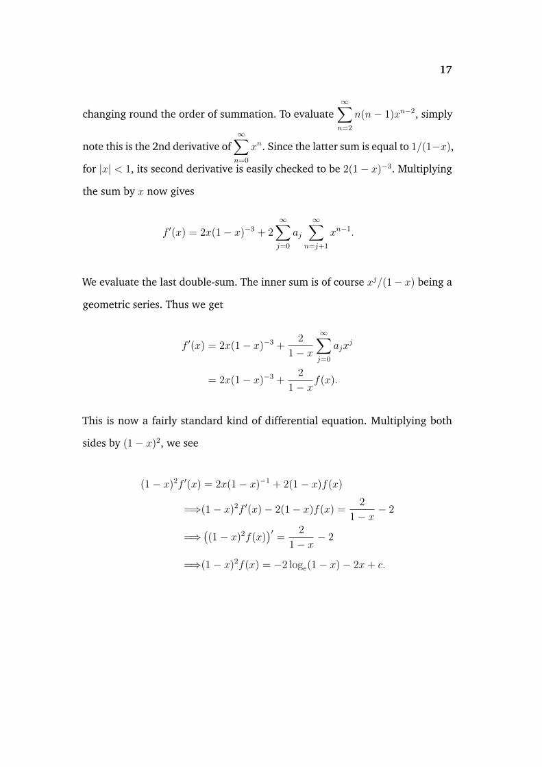
17
changing round the order of summation. To evaluate∞∑n=2
n(n− 1)xn−2, simply
note this is the 2nd derivative of∞∑n=0
xn. Since the latter sum is equal to 1/(1−x),
for |x| < 1, its second derivative is easily checked to be 2(1− x)−3. Multiplying
the sum by x now gives
f ′(x) = 2x(1− x)−3 + 2∞∑j=0
aj
∞∑n=j+1
xn−1.
We evaluate the last double-sum. The inner sum is of course xj/(1− x) being a
geometric series. Thus we get
f ′(x) = 2x(1− x)−3 +2
1− x
∞∑j=0
ajxj
= 2x(1− x)−3 +2
1− xf(x).
This is now a fairly standard kind of differential equation. Multiplying both
sides by (1− x)2, we see
(1− x)2f ′(x) = 2x(1− x)−1 + 2(1− x)f(x)
=⇒(1− x)2f ′(x)− 2(1− x)f(x) =2
1− x− 2
=⇒((1− x)2f(x)
)′=
2
1− x− 2
=⇒(1− x)2f(x) = −2 loge(1− x)− 2x+ c.
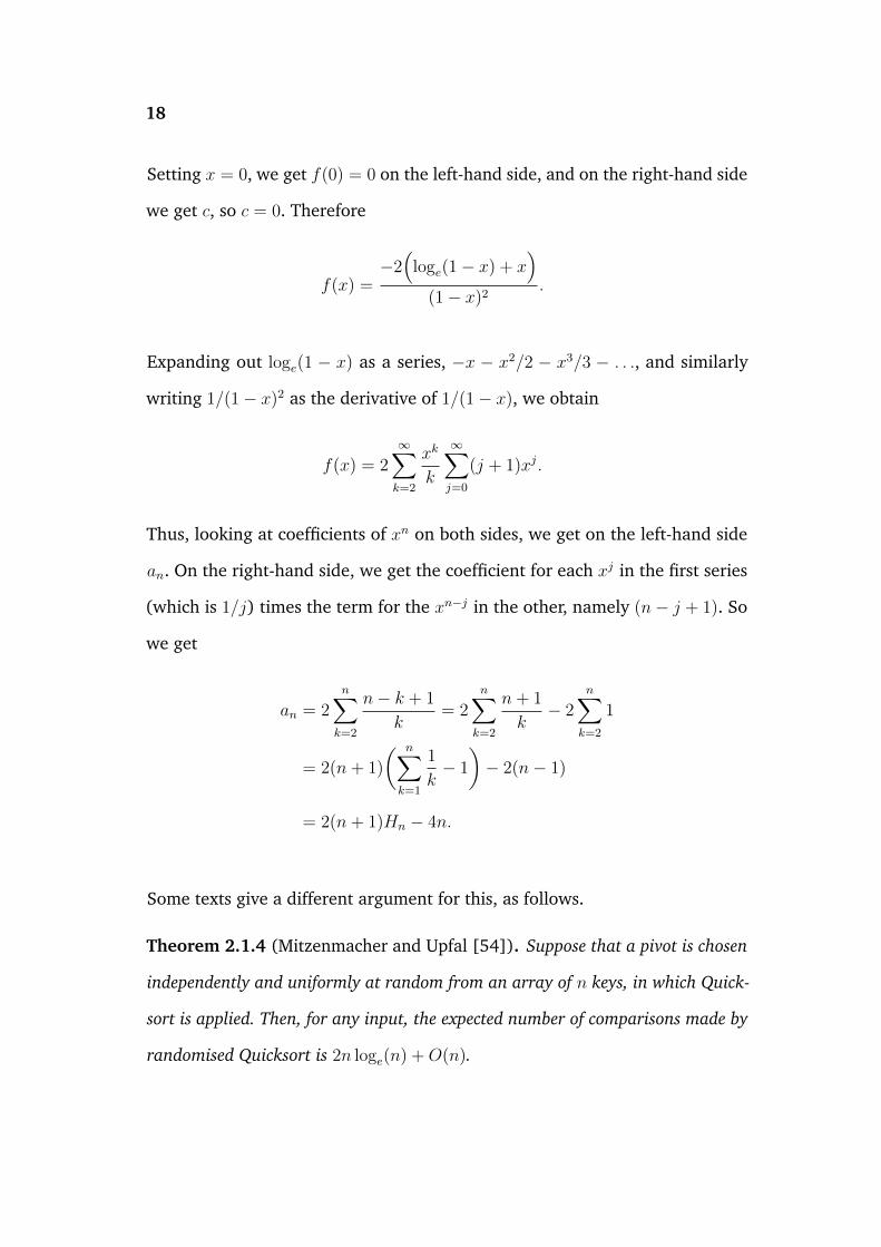
18
Setting x = 0, we get f(0) = 0 on the left-hand side, and on the right-hand side
we get c, so c = 0. Therefore
f(x) =−2(
loge(1− x) + x)
(1− x)2.
Expanding out loge(1 − x) as a series, −x − x2/2 − x3/3 − . . ., and similarly
writing 1/(1− x)2 as the derivative of 1/(1− x), we obtain
f(x) = 2∞∑k=2
xk
k
∞∑j=0
(j + 1)xj.
Thus, looking at coefficients of xn on both sides, we get on the left-hand side
an. On the right-hand side, we get the coefficient for each xj in the first series
(which is 1/j) times the term for the xn−j in the other, namely (n− j + 1). So
we get
an = 2n∑k=2
n− k + 1
k= 2
n∑k=2
n+ 1
k− 2
n∑k=2
1
= 2(n+ 1)
( n∑k=1
1
k− 1
)− 2(n− 1)
= 2(n+ 1)Hn − 4n.
Some texts give a different argument for this, as follows.
Theorem 2.1.4 (Mitzenmacher and Upfal [54]). Suppose that a pivot is chosen
independently and uniformly at random from an array of n keys, in which Quick-
sort is applied. Then, for any input, the expected number of comparisons made by
randomised Quicksort is 2n loge(n) +O(n).
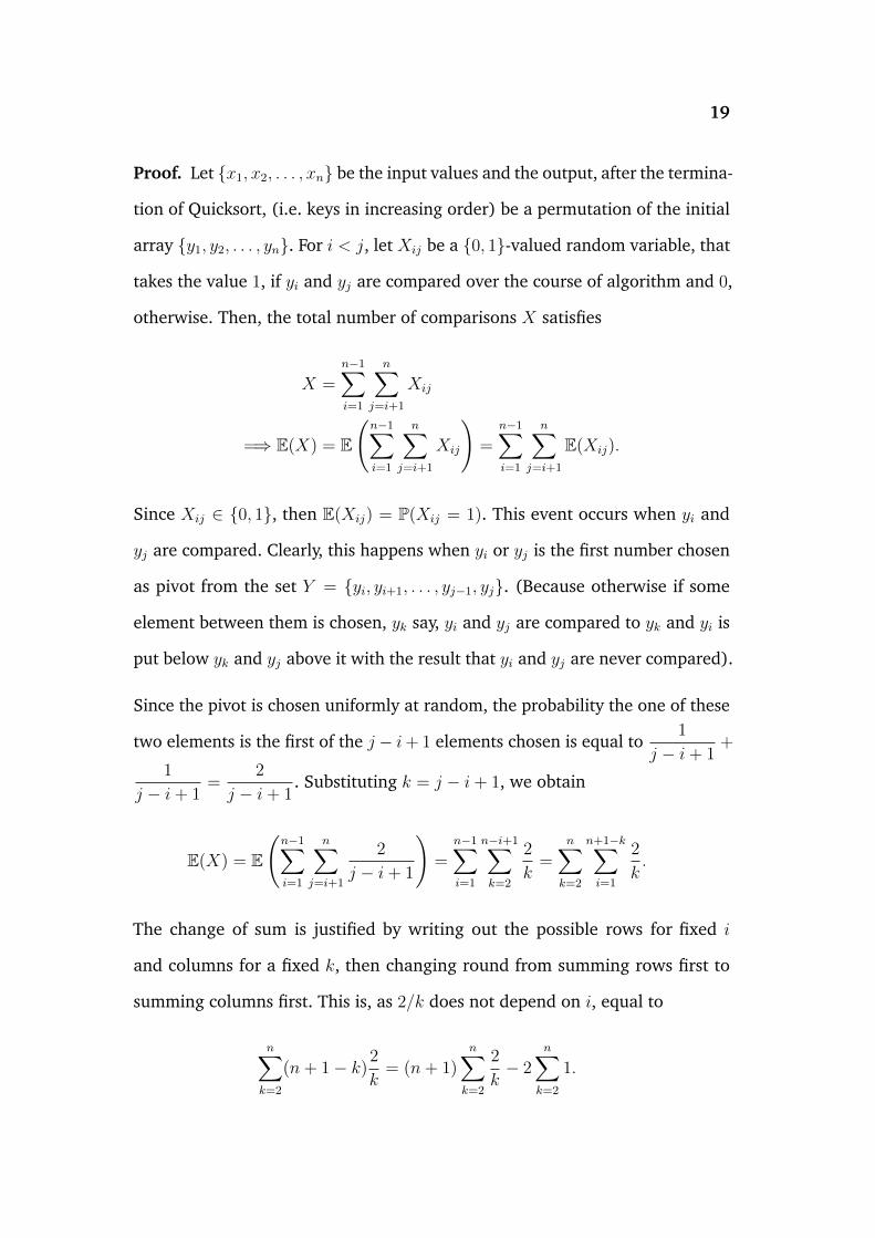
19
Proof. Let x1, x2, . . . , xn be the input values and the output, after the termina-
tion of Quicksort, (i.e. keys in increasing order) be a permutation of the initial
array y1, y2, . . . , yn. For i < j, let Xij be a 0, 1-valued random variable, that
takes the value 1, if yi and yj are compared over the course of algorithm and 0,
otherwise. Then, the total number of comparisons X satisfies
X =n−1∑i=1
n∑j=i+1
Xij
=⇒ E(X) = E
(n−1∑i=1
n∑j=i+1
Xij
)=
n−1∑i=1
n∑j=i+1
E(Xij).
Since Xij ∈ 0, 1, then E(Xij) = P(Xij = 1). This event occurs when yi and
yj are compared. Clearly, this happens when yi or yj is the first number chosen
as pivot from the set Y = yi, yi+1, . . . , yj−1, yj. (Because otherwise if some
element between them is chosen, yk say, yi and yj are compared to yk and yi is
put below yk and yj above it with the result that yi and yj are never compared).
Since the pivot is chosen uniformly at random, the probability the one of these
two elements is the first of the j − i+ 1 elements chosen is equal to1
j − i+ 1+
1
j − i+ 1=
2
j − i+ 1. Substituting k = j − i+ 1, we obtain
E(X) = E
(n−1∑i=1
n∑j=i+1
2
j − i+ 1
)=
n−1∑i=1
n−i+1∑k=2
2
k=
n∑k=2
n+1−k∑i=1
2
k.
The change of sum is justified by writing out the possible rows for fixed i
and columns for a fixed k, then changing round from summing rows first to
summing columns first. This is, as 2/k does not depend on i, equal to
n∑k=2
(n+ 1− k)2
k= (n+ 1)
n∑k=2
2
k− 2
n∑k=2
1.
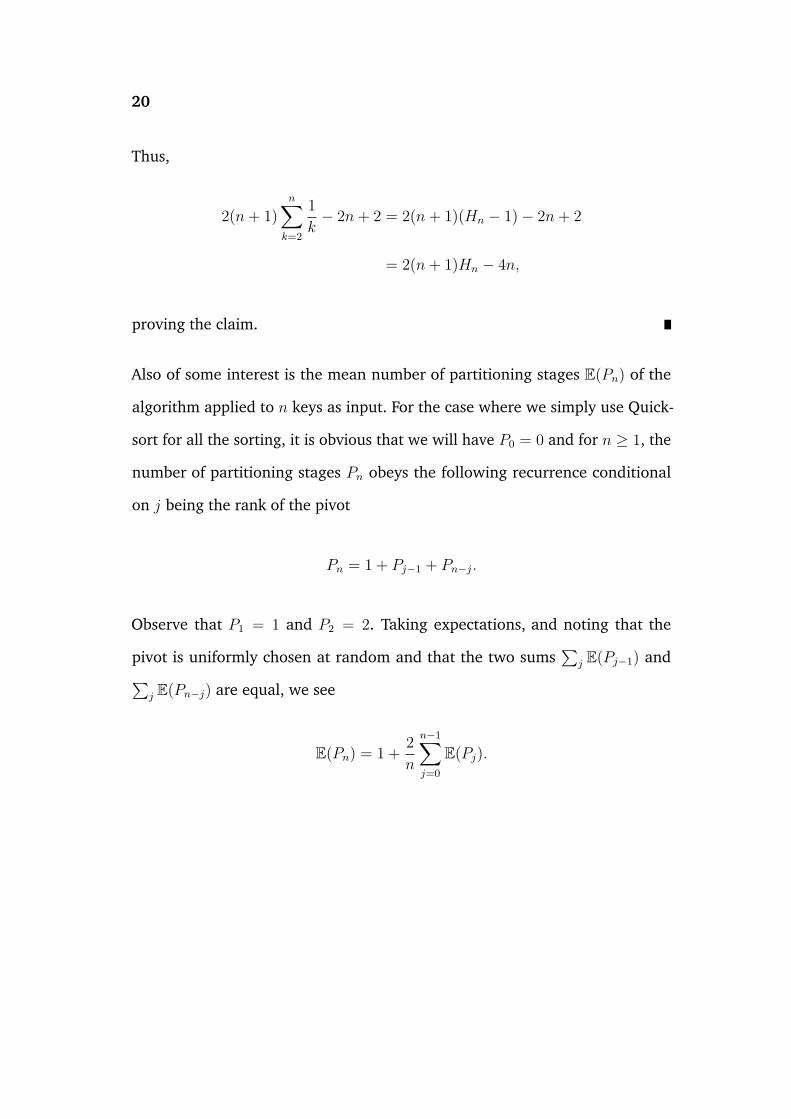
20
Thus,
2(n+ 1)n∑k=2
1
k− 2n+ 2 = 2(n+ 1)(Hn − 1)− 2n+ 2
= 2(n+ 1)Hn − 4n,
proving the claim.
Also of some interest is the mean number of partitioning stages E(Pn) of the
algorithm applied to n keys as input. For the case where we simply use Quick-
sort for all the sorting, it is obvious that we will have P0 = 0 and for n ≥ 1, the
number of partitioning stages Pn obeys the following recurrence conditional
on j being the rank of the pivot
Pn = 1 + Pj−1 + Pn−j.
Observe that P1 = 1 and P2 = 2. Taking expectations, and noting that the
pivot is uniformly chosen at random and that the two sums∑
j E(Pj−1) and∑j E(Pn−j) are equal, we see
E(Pn) = 1 +2
n
n−1∑j=0
E(Pj).
21
Multiplying both sides by n and differencing the recurrence relation, as we did
for the derivation of the expected number of comparisons, we have
nE(Pn)− (n− 1)E(Pn−1) = 1 + 2E(Pn−1)
=⇒ E(Pn)
n+ 1=
1
n(n+ 1)+
E(Pn−1)
n
=⇒ E(Pn) = (n+ 1)
( n∑j=2
(1
j− 1
j + 1
)+
1
2
).
Finally, E(Pn) = n.
2.2 Expected number of exchanges
Here we consider the number of exchanges or swaps performed by the algo-
rithm, which is mentioned by Hoare [30] as a relevant quantity. We assume
that each swap has a fixed cost and as in the previous section, we assume that
the keys are distinct and that all n! permutations are equally likely to be the
input: this in particular implies that the pivot is chosen uniformly at random
from the array.
We should specify the partitioning procedure. Assume that we have to sort n
distinct keys, where their locations in the array are numbered from left to right
by 1, 2, . . . , n. Set two pointers i← 1 and j ← n− 1 and select the element at
location n as a pivot. First, compare the element at location 1 with the pivot.
If this key is less than the pivot, increase i by one until an element greater
than the pivot is found. If an element greater than the pivot is found, stop and
compare the element at location n− 1 with the pivot. If this key is greater than
the pivot, then decrease j by one and compare the next element to the pivot.
22
If an element less than the pivot is found, then the j pointer stops its scan and
the keys that the two pointers refer are exchanged.
Increase i by one, decrease j by one and in the same manner continue the
scanning of the array until i ≥ j. At the end of the partitioning operation,
the pivot is placed in its final position k, where 1 ≤ k ≤ n, and Quicksort is
recursively invoked to sort the subarray of k − 1 keys less than the pivot and
the subarray of n− k keys greater than the pivot [29, 30].
Note that the probability of a key being greater than the pivot is
n− kn− 1
.
The number of keys which are greater than pivot, and were moved during
partition isn− kn− 1
· (k − 1).
Therefore, considering also that pivots are uniformly chosen and noting that
we have to count the final swap with the pivot at the end of partition operation,
we obtain
n∑k=1
(n− k)(k − 1)
n(n− 1)+ 1 =
n
6+
2
3.
Let Sn be the total number of exchanges, when the algorithm is applied to an
array of n distinct keys. We have that S0 = S1 = 0 and for n ≥ 2, the following
recurrence holds
Sn = “Number of exchanges during partition routine” + Sk−1 + Sn−k.
23
Since the pivot is chosen uniformly at random, the recurrence for the expected
number of exchanges is
E(Sn) =n
6+
2
3+
1
n
n∑k=1
(E(Sk−1) + E(Sn−k)
)=⇒ E(Sn) =
n
6+
2
3+
2
n
n−1∑k=0
E(Sk).
This recurrence relation is similar to the recurrences about the mean number
of comparisons and will be solved by the same way. Subtracting (n− 1)E(Sn−1)
from nE(Sn), the recurrence becomes
nE(Sn)− (n− 1)E(Sn−1) =2n+ 3
6+ 2E(Sn−1)
=⇒ E(Sn)
n+ 1=
2n+ 3
6n(n+ 1)+
E(Sn−1)
n.
Telescoping, the last relation yields
E(Sn)
n+ 1=
n∑j=3
2j + 3
6j(j + 1)+
1
3=
n∑j=3
1
3(j + 1)+
n∑j=3
1
2j(j + 1)+
1
3
=1
3
n∑j=3
1
j + 1+
1
2
(n∑j=3
1
j−
n∑j=3
1
j + 1
)+
1
3
=1
3
(Hn+1 −
11
6
)+
1
2
(1
3− 1
n+ 1
)+
1
3.
Tidying up, the average number of exchanges in course of the algorithm is
E(Sn) =(n+ 1)Hn
3− n
9− 5
18.
Its asymptotic value isn loge(n)
3.
24
It follows that asymptotically the mean number of exchanges is about 1/6 of
the average number of comparisons.
In a variant of the algorithm analysed in [46] and [63], which we briefly
mentioned in the introduction, partitioning of n keys takes n+ 1 comparisons
and subfiles of m or fewer elements are sorted using insertion sort. Then the
average number of comparisons, partitioning stages and exchanges respectively,
are
E(Cn) = (n+ 1)(2Hn+1 − 2Hm+2 + 1),
E(Pn) = 2 · n+ 1
m+ 2− 1 and
E(Sn) = (n+ 1)(1
3Hn+1 −
1
3Hm+2 +
1
6− 1
m+ 2
)+
1
2, for n > m.
Form = 0, we obtain the average quantities when there is no switch to insertion
sort. Note that in this case the expected costs are
E(Cn) = 2(n+ 1)Hn − 2n,
E(Pn) = n and
E(Sn) =2(n+ 1)Hn − 5n
6.
2.3 Variance
We now similarly discuss the variance of the number of comparisons in Quick-
sort. Although the result has been known for many years – see [46], exercise
6.2.2-8 for an outline – there is not really a full version of all the details written
down conveniently that we are aware of, so we have provided such an account
25
– this summary has been put on arXiv, [33]. The sources [43], [55] and [63]
were useful in putting the argument together. Again, generating functions will
be used. The result is:
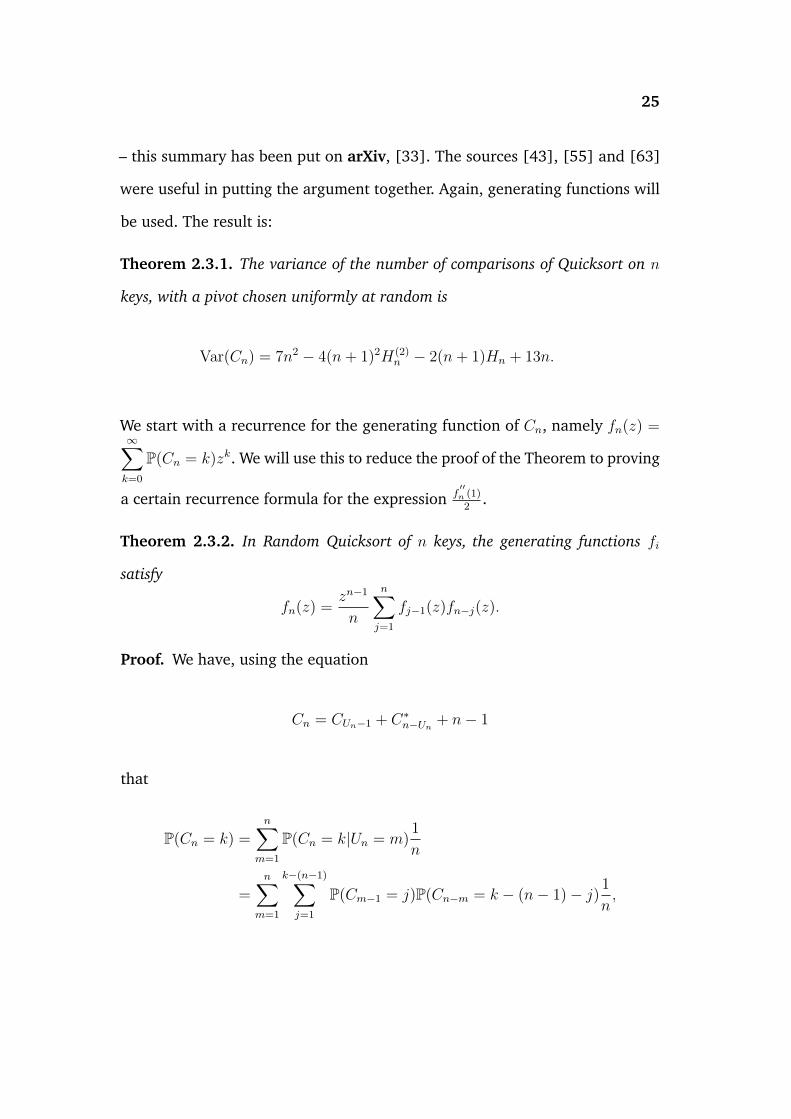
Theorem 2.3.1. The variance of the number of comparisons of Quicksort on n
keys, with a pivot chosen uniformly at random is
Var(Cn) = 7n2 − 4(n+ 1)2H(2)n − 2(n+ 1)Hn + 13n.
We start with a recurrence for the generating function of Cn, namely fn(z) =∞∑k=0
P(Cn = k)zk. We will use this to reduce the proof of the Theorem to proving
a certain recurrence formula for the expression f′′n (1)2
.
Theorem 2.3.2. In Random Quicksort of n keys, the generating functions fi
satisfy
fn(z) =zn−1
n
n∑j=1
fj−1(z)fn−j(z).
Proof. We have, using the equation
Cn = CUn−1 + C∗n−Un + n− 1
that
P(Cn = k) =n∑
m=1
P(Cn = k|Un = m)1
n
=n∑
m=1
k−(n−1)∑j=1
P(Cm−1 = j)P(Cn−m = k − (n− 1)− j) 1
n,
26
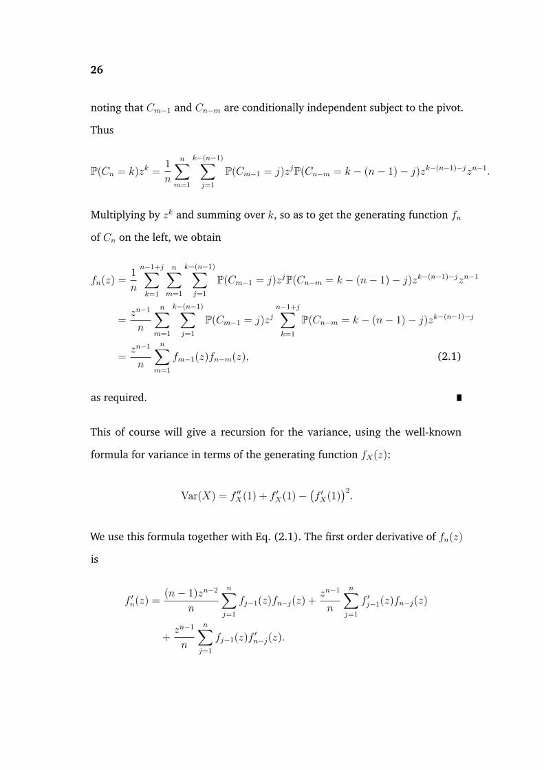
noting that Cm−1 and Cn−m are conditionally independent subject to the pivot.
Thus
P(Cn = k)zk =1
n
n∑m=1
k−(n−1)∑j=1
P(Cm−1 = j)zjP(Cn−m = k − (n− 1)− j)zk−(n−1)−jzn−1.
Multiplying by zk and summing over k, so as to get the generating function fn
of Cn on the left, we obtain
fn(z) =1
n
n−1+j∑k=1
n∑m=1
k−(n−1)∑j=1
P(Cm−1 = j)zjP(Cn−m = k − (n− 1)− j)zk−(n−1)−jzn−1
=zn−1
n
n∑m=1
k−(n−1)∑j=1
P(Cm−1 = j)zjn−1+j∑k=1
P(Cn−m = k − (n− 1)− j)zk−(n−1)−j
=zn−1
n
n∑m=1
fm−1(z)fn−m(z), (2.1)
as required.
This of course will give a recursion for the variance, using the well-known
formula for variance in terms of the generating function fX(z):
Var(X) = f ′′X(1) + f ′X(1)−(f ′X(1)
)2.
We use this formula together with Eq. (2.1). The first order derivative of fn(z)
is
f ′n(z) =(n− 1)zn−2
n
n∑j=1
fj−1(z)fn−j(z) +zn−1
n
n∑j=1
f ′j−1(z)fn−j(z)
+zn−1
n
n∑j=1
fj−1(z)f ′n−j(z).
27
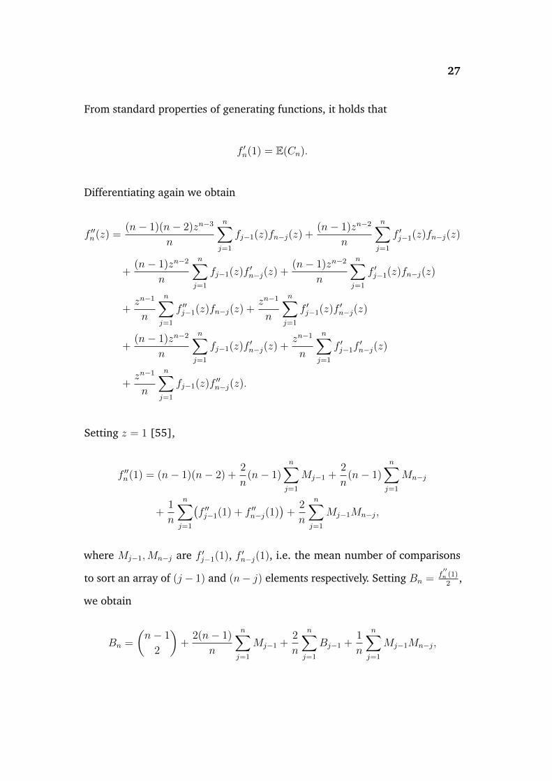
From standard properties of generating functions, it holds that
f ′n(1) = E(Cn).
Differentiating again we obtain
f ′′n(z) =(n− 1)(n− 2)zn−3
n
n∑j=1
fj−1(z)fn−j(z) +(n− 1)zn−2
n
n∑j=1
f ′j−1(z)fn−j(z)
+(n− 1)zn−2
n
n∑j=1
fj−1(z)f ′n−j(z) +(n− 1)zn−2
n
n∑j=1
f ′j−1(z)fn−j(z)
+zn−1
n
n∑j=1
f ′′j−1(z)fn−j(z) +zn−1
n
n∑j=1
f ′j−1(z)f ′n−j(z)
+(n− 1)zn−2
n
n∑j=1
fj−1(z)f ′n−j(z) +zn−1
n
n∑j=1
f ′j−1f′n−j(z)
+zn−1
n
n∑j=1
fj−1(z)f ′′n−j(z).
Setting z = 1 [55],
f ′′n(1) = (n− 1)(n− 2) +2
n(n− 1)
n∑j=1
Mj−1 +2
n(n− 1)
n∑j=1
Mn−j
+1
n
n∑j=1
(f ′′j−1(1) + f ′′n−j(1)
)+
2
n
n∑j=1
Mj−1Mn−j,
where Mj−1,Mn−j are f ′j−1(1), f ′n−j(1), i.e. the mean number of comparisons
to sort an array of (j − 1) and (n− j) elements respectively. Setting Bn = f′′n (1)2
,
we obtain
Bn =
(n− 1
2
)+
2(n− 1)
n
n∑j=1
Mj−1 +2
n
n∑j=1
Bj−1 +1
n
n∑j=1
Mj−1Mn−j,
28
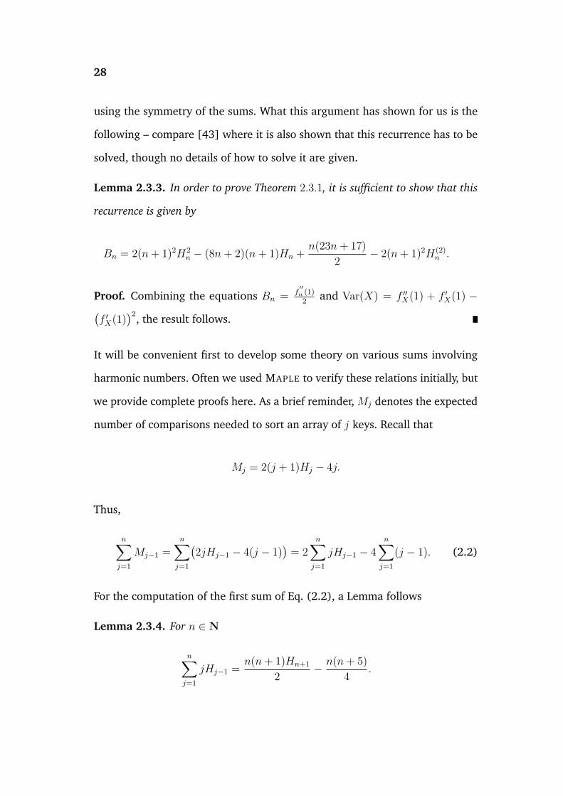
using the symmetry of the sums. What this argument has shown for us is the
following – compare [43] where it is also shown that this recurrence has to be
solved, though no details of how to solve it are given.
Lemma 2.3.3. In order to prove Theorem 2.3.1, it is sufficient to show that this
recurrence is given by
Bn = 2(n+ 1)2H2n − (8n+ 2)(n+ 1)Hn +
n(23n+ 17)
2− 2(n+ 1)2H(2)
n .
Proof. Combining the equations Bn = f′′n (1)2
and Var(X) = f ′′X(1) + f ′X(1) −(f ′X(1)
)2, the result follows.
It will be convenient first to develop some theory on various sums involving
harmonic numbers. Often we used MAPLE to verify these relations initially, but
we provide complete proofs here. As a brief reminder, Mj denotes the expected
number of comparisons needed to sort an array of j keys. Recall that
Mj = 2(j + 1)Hj − 4j.
Thus,
n∑j=1
Mj−1 =n∑j=1
(2jHj−1 − 4(j − 1)
)= 2
n∑j=1
jHj−1 − 4n∑j=1
(j − 1). (2.2)
For the computation of the first sum of Eq. (2.2), a Lemma follows
Lemma 2.3.4. For n ∈ N
n∑j=1
jHj−1 =n(n+ 1)Hn+1
2− n(n+ 5)
4.

29
Proof. The sum can be written as
n∑j=1
jHj−1 = 2 + 3
(1 +
1
2
)+ . . .+ n
(1 +
1
2+ . . .+
1
n− 1
)= Hn−1(1 + 2 + . . .+ n)−
(1 +
1 + 2
2+ . . .+
1 + 2 + . . .+ n− 1
n− 1
)=n(n+ 1)
2Hn−1 −
n−1∑j=1
(∑ji=1 i
j
)=n(n+ 1)
2Hn−1 −
1
2
(n(n+ 1)
2− 1
).
The last equation can be easily seen to be equivalent with the statement of the
Lemma.
Thus we can find out about the sum of the Mjs, that it holds for n ∈ N
Corollary 2.3.5.
n∑j=1
Mj−1 = n(n+ 1)Hn+1 −5n2 + n
2.
Proof. Using Lemma 2.3.4 and Eq. (2.2), the proof is immediate.
Now, we will compute the termn∑j=1
Mj−1Mn−j. We shall use three Lemmas for
the following proof.
Lemma 2.3.6. For n ∈ N, it holds that
n∑j=1
Mj−1Mn−j = 4n∑j=1
jHj−1(n− j + 1)Hn−j
− 8
3n(n2 − 1)Hn+1 +
44n
9(n2 − 1).
30
Proof. To do this, we will again use the formula obtained previously for Mj.
We have
n∑j=1
Mj−1Mn−j =n∑j=1
((2jHj−1 − 4j + 4
)(2(n− j + 1)Hn−j − 4n+ 4j
))
= 4n∑j=1
jHj−1(n− j + 1)Hn−j − 8nn∑j=1
jHj−1 + 8n∑j=1
j2Hj−1
− 8n∑j=1
j(n− j + 1)Hn−j + 16nn∑j=1
j − 16n∑j=1
j2
+ 8n∑j=1
(n− j + 1)Hn−j − 16n2 + 16n∑j=1
j.
We need to work out the value ofn∑j=1
j2Hj−1:
Lemma 2.3.7. For n ∈ N holds
n∑j=1
j2Hj−1 =6n(n+ 1)(2n+ 1)Hn+1 − n(n+ 1)(4n+ 23)
36.
Proof. Using the same reasoning as in Lemma 2.3.4,
n∑j=1
j2Hj−1 = 22 + 32
(1 +
1
2
)+ . . .+ n2
(1 +
1
2+ . . .+
1
n− 1
)= Hn−1(12 + 22 + . . .+ n2)
−(
1 +12 + 22
2+ . . .+
12 + 22 + . . .+ (n− 1)2
n− 1
)=n(n+ 1)(2n+ 1)
6Hn−1 −
n−1∑j=1
(∑ji=1 i
2
j
)=n(n+ 1)(2n+ 1)
6Hn−1 −
1
36(4n3 + 3n2 − n− 6),
completing the proof.
31
We also need to computen∑j=1
j(n− j + 1)Hn−j. A Lemma follows
Lemma 2.3.8. For n ∈ N
n∑j=1
j(n− j + 1)Hn−j =6nHn+1(n2 + 3n+ 2)− 5n3 − 27n2 − 22n
36.
Proof. We can write j = n+ 1− (n− j + 1). Then, substituting k = n− j + 1
n∑j=1
j(n− j + 1)Hn−j =n∑j=1
((n+ 1)− (n− j + 1)
)(n− j + 1)Hn−j
= (n+ 1)n∑j=1
(n− j + 1)Hn−j −n∑j=1
(n− j + 1)2Hn−j
= (n+ 1)n∑k=1
kHk−1 −n∑k=1
k2Hk−1.
These sums can be computed using Lemmas 2.3.4 and 2.3.7.
32
In the same manner we shall computen∑j=1
(n− j + 1)Hn−j. Changing variables,
the expression becomesn∑k=1
kHk−1. Using the previous results, we have
n∑j=1
Mj−1Mn−j = 4n∑j=1
jHj−1(n− j + 1)Hn−j − 8n
(n(n+ 1)Hn+1
2− n(n+ 5)
4
)
+ 8
(6n(n+ 1)(2n+ 1)Hn+1 − n(n+ 1)(4n+ 23)
36
)+ 16n
n∑j=1
j
− 8
(6nHn+1(n2 + 3n+ 2)− 5n3 − 27n2 − 22n
36
)− 16
n∑j=1
j2
+ 8
(n(n+ 1)Hn+1
2− n(n+ 5)
4
)− 16n2 + 16
n∑j=1
j
= 4n∑j=1
jHj−1(n− j + 1)Hn−j − 4n(n+ 1)(n− 1)Hn+1
+4
3n(n2 − 1)Hn+1 +
176n3
36− 176n
36,
finishing the proof of Lemma 2.3.6.
After some tedious calculations, the recurrence relation becomes
Bn =
4n∑j=1
jHj−1(n− j + 1)Hn−j
n+
2
n
n∑j=1
Bj−1 +−9n2 + 5n+ 4
2
− 2
3(n2 − 1)Hn+1 +
44
9(n2 − 1).

33
Subtracting nBn from (n+ 1)Bn+1,
(n+ 1)Bn+1 − nBn
= 4
(n+1∑j=1
jHj−1(n− j + 2)Hn+1−j −n∑j=1
jHj−1(n− j + 1)Hn−j
)+ 2Bn + (n+ 1)
−9(n+ 1)2 + 5(n+ 1) + 4
2− n−9n2 + 5n+ 4
2
− (n+ 1)2
3
((n+ 1)2 − 1
)Hn+2 +
2
3n(n2 − 1)Hn+1
+ (n+ 1)44
9
((n+ 1)2 − 1
)− n44
9(n2 − 1)
= 4
( n∑j=1
jHj−1(n− j + 2)Hn+1−j −n∑j=1
jHj−1(n− j + 1)Hn−j
)+ 2Bn −
27n2 + 17n
2− 2
3n(n+ 1)(n+ 2)Hn+2
+2
3nHn+1(n2 − 1) +
44n(n+ 1)
3.
We obtain
(n+ 1)Bn+1 − nBn = 4
( n∑j=1
jHj−1 +n∑j=1
jHj−1Hn−j+1
)+ 2Bn − 2n(n+ 1)Hn+1 +
1
2n(n+ 11).
We have to work out the following sum
n∑j=1
jHj−1Hn+1−j.
34
We note that
n∑j=1
jHj−1Hn+1−j = 2H1Hn−1 + 3H2Hn−2 + . . .+ (n− 1)Hn−2H2 + nHn−1H1
=n+ 2
2
n∑j=1
HjHn−j. (2.3)
Sedgewick [63], presents and proves the following result:
Lemma 2.3.9.
n∑i=1
HiHn+1−i = (n+ 2)(H2n+1 −H
(2)n+1)− 2(n+ 1)(Hn+1 − 1).
Proof. By the definition of harmonic numbers, we have
n∑i=1
HiHn+1−i =n∑i=1
Hi
n+1−i∑j=1
1
j
and the above equation becomes
n∑j=1
1
j
n+1−j∑i=1
Hi =n∑j=1
1
j
((n+ 2− j)Hn+1−j − (n+ 1− j)
), (2.4)
using the identity [44],
n∑j=1
Hj = (n+ 1)Hn − n.
35
Eq. (2.4) can be written as
(n+ 2)n∑j=1
Hn+1−j
j−
n∑j=1
Hn+1−j − (n+ 1)Hn + n
= (n+ 2)n∑j=1
Hn+1−j
j−((n+ 1)Hn − n
)− (n+ 1)Hn + n
= (n+ 2)n∑j=1
Hn+1−j
j− 2(n+ 1)(Hn+1 − 1).
It can be easily verified that
n∑j=1
Hn+1−j
j=
n∑j=1
Hn−j
j+
n∑j=1
1
j(n+ 1− j)
=n−1∑j=1
Hn−j
j+ 2
Hn
n+ 1. (2.5)
Making repeated use of Eq. (2.5), we obtain the identity
n∑j=1
Hn+1−j
j= 2
n∑k=1
Hk
k + 1.
We have then
2n∑k=1
Hk
k + 1= 2
n+1∑k=2
Hk−1
k= 2
n+1∑k=1
Hk−1
k= 2
n+1∑k=1
Hk
k− 2
n+1∑k=1
1
k2
= 2n+1∑k=1
k∑j=1
1
jk− 2H
(2)n+1 = 2
n+1∑j=1
n+1∑k=j
1
jk− 2H
(2)n+1
= 2n+1∑k=1
n+1∑j=k
1
kj− 2H
(2)n+1.

36
The order of summation was interchanged. We can sum on all j and for k = j,
we must count this term twice. We obtain
2n∑k=1
Hk
k + 1=
n+1∑k=1
(n+1∑j=1
1
kj+
1
k2
)− 2H
(2)n+1 = H2
n+1 −H(2)n+1. (2.6)
Finally
n∑i=1
HiHn+1−i = (n+ 2)(H2n+1 −H
(2)n+1)− 2(n+ 1)(Hn+1 − 1).
The following Corollary is a direct consequence of Eq. (2.5) and (2.6).
Corollary 2.3.10. For n ∈ N, it holds
H2n+1 −H
(2)n+1 = 2
n∑j=1
Hj
j + 1.
Proof.
H2n+1 −H
(2)n+1 = H2
n −H(2)n + 2
Hn
n+ 1and by iteration,
H2n+1 −H
(2)n+1 = 2
n∑j=1
Hj
j + 1.
We will use the above Lemma and Corollary in our analysis. We have that
n∑i=1
HiHn+1−i =n∑i=1
(Hi
(Hn−i +
1
n+ 1− i
))=
n∑i=1
HiHn−i +n∑i=1
Hi
n+ 1− i.
The second sum substituting j = n+ 1− i becomes
n∑i=1
Hi
n+ 1− i=
n∑j=1
Hn+1−j
j.
37
As we have seen it is equal to
n∑j=1
Hn+1−j
j= 2
n∑j=1
Hj
j + 1= H2
n+1 −H(2)n+1.
Hence, by Lemma 2.3.9,
n∑j=1
HjHn−j = (n+ 2)(H2n+1 −H
(2)n+1)− 2(n+ 1)(Hn+1 − 1)− (H2
n+1 −H(2)n+1)
= (n+ 1)((H2
n+1 −H(2)n+1)− 2(Hn+1 − 1)
).
Using the above result and Eq. (2.3), we have
n∑j=1
jHj−1Hn+1−j =
(n+ 2
2
)((H2
n −H(2)n ) +
2n(1−Hn)
n+ 1
).
Having worked out all the expressions involved in the following relation
(n+ 1)Bn+1 − nBn = 4
( n∑j=1
jHj−1 +n∑j=1
jHj−1Hn−j+1
)+ 2Bn − 2n(n+ 1)Hn+1 +
1
2n(n+ 11).
This becomes
(n+ 1)Bn+1 − nBn
= 4
(n(n+ 1)Hn+1
2− n(n+ 5)
4+
(n+ 2
2
)((H2
n+1 −H(2)n+1)− 2(Hn+1 − 1)
))
+ 2Bn − 2n(n+ 1)Hn+1 +1
2n(n+ 11)
= 2(n+ 1)(n+ 2)(H2n+1 −H
(2)n+1)− 4(n+ 1)(n+ 2)(Hn+1 − 1)− n(n− 1)
2+ 2Bn.
38
Dividing both sides by (n+ 1)(n+ 2) and unwinding the recurrence,
Bn
n+ 1=B0
1+ 2
n∑i=1
(H2i −H
(2)i )− 4
n∑i=1
(Hi − 1)−n∑i=1
(i− 1)(i− 2)
2i(i+ 1).
Hence
Bn
n+ 1= 2(n+ 1)(H2
n −H(2)n ) + 4n− 4nHn − 4
((n+ 1)Hn − 2n
)−
n∑i=1
(i+ 2
2i− 3
i+ 1
)= 2(n+ 1)(H2
n −H(2)n )−Hn(8n+ 2) +
23n
2− 3 +
3
n+ 1
= 2(n+ 1)(H2n −H(2)
n )−Hn(8n+ 2) +23n2 + 17n
2(n+ 1).
Finally, multiplying by (n+ 1) we obtain
Bn = 2(n+ 1)2(H2n −H(2)
n )−Hn(n+ 1)(8n+ 2) +23n2 + 17n
2.
Consequently, by Lemma 2.3.3 the variance of the number of comparisons of
randomised Quicksort is
7n2 − 4(n+ 1)2H(2)n − 2(n+ 1)Hn + 13n,
completing the proof of Theorem 2.3.1.
2.4 “Divide and Conquer” recurrences
We have computed the mean and variance of the number of comparisons made
by Quicksort that mainly contribute to its time complexity. Because of the sim-
39
ple structure of the algorithm (dividing into smaller subproblems) we can in
fact approach many other related problems in the same spirit. Let F (n) denote
the expected value of some random variable associated with randomised Quick-
sort and T (n) be the average value of the “toll function”, which is the needed
cost to divide the problem into two simpler subproblems. Then F (n) is equal to
the contribution T (n), plus the measures required sort the resulting subarrays
of (i − 1) and (n − i) elements, where the pivot i can be any key of the array
with equal probability.
Thus, the recurrence relation is
F (n) = T (n) +1
n
n∑i=1
(F (i− 1) + F (n− i))
= T (n) +2
n
n∑i=1
F (i− 1).
This is the general type of recurrences arising in the analysis of Quicksort, which
can be manipulated using the difference method or by generating functions.
Since an empty array or an one having a unique key is trivially solved, the
initial values of the recurrence is
F (0) = F (1) = 0.
The first method leads to the elimination of the sum, by subtracting (n−1)F (n−
1) from nF (n) – see [46]. The recurrence becomes
nF (n)− (n− 1)F (n− 1) = nT (n)− (n− 1)T (n− 1) + 2F (n− 1)
40
and dividing by n(n+ 1) we have
F (n)
n+ 1=nT (n)− (n− 1)T (n− 1)
n(n+ 1)+F (n− 1)
n.
This recurrence can be immediately solved by “unfolding” its terms. The general
solution is
F (n) = (n+ 1)
(n∑j=3
jT (j)− (j − 1)T (j − 1)
j(j + 1)+F (2)
3
)
= (n+ 1)
(n∑j=3
jT (j)− (j − 1)T (j − 1)
j(j + 1)+T (2)
3
).
When the sorting of subarrays of m keys or less is done by insertion sort, the
solution of the recurrence is
F (n) = (n+ 1)
( n∑j=m+2
jT (j)− (j − 1)T (j − 1)
j(j + 1)+F (m+ 1)
m+ 2
)
= (n+ 1)
( n∑j=m+2
jT (j)− (j − 1)T (j − 1)
j(j + 1)+T (m+ 1)
m+ 2
),
since n− 1 > m.
Another classic approach, which is more transparent and elegant, is the appli-
cation of generating functions. The recurrence is transformed to a differential
equation, which is then solved. The function is written in terms of series and
the extracted coefficient is the solution. Multiplying by nxn and then summing
with respect to n, in order to obtain the generating function G(x) =∞∑n=0
F (n)xn,
we have
∞∑n=0
nF (n)xn =∞∑n=0
nT (n)xn + 2∞∑n=0
n∑i=1
F (i− 1)xn.
41
The double sum is equal to
∞∑n=0
n∑i=1
F (i− 1)xn = G(x)∞∑n=1
xn =xG(x)
1− x
and the differential equation is
xG′(x) =∞∑n=0
nT (n)xn +2xG(x)
1− x.
Cancelling out x and multiplying by (1− x)2,
G′(x)(1− x)2 = (1− x)2
∞∑n=1
nT (n)xn−1 + 2(1− x)G(x)
(G(x)(1− x)2
)′= (1− x)2
∞∑n=1
nT (n)xn−1
=⇒ G(x)(1− x)2 =
∫(1− x)2
∞∑n=1
nT (n)xn−1 dx+ C
=⇒ G(x) =
∫(1− x)2
∞∑n=1
nT (n)xn−1 dx+ C
(1− x)2,
where C is constant, which can be found using the initial condition G(0) = 0.
The solution then is being written as power series and the coefficient sequence
found is the expected sought cost.
Now, one can obtain any expected cost of the algorithm, just by using these
results. The “toll function” will be different for each case. Plugging in the
average value, the finding becomes a matter of simple operations. This type of
analysis unifies the recurrences of Quicksort into a single one and provides an
intuitive insight of the algorithm.
42
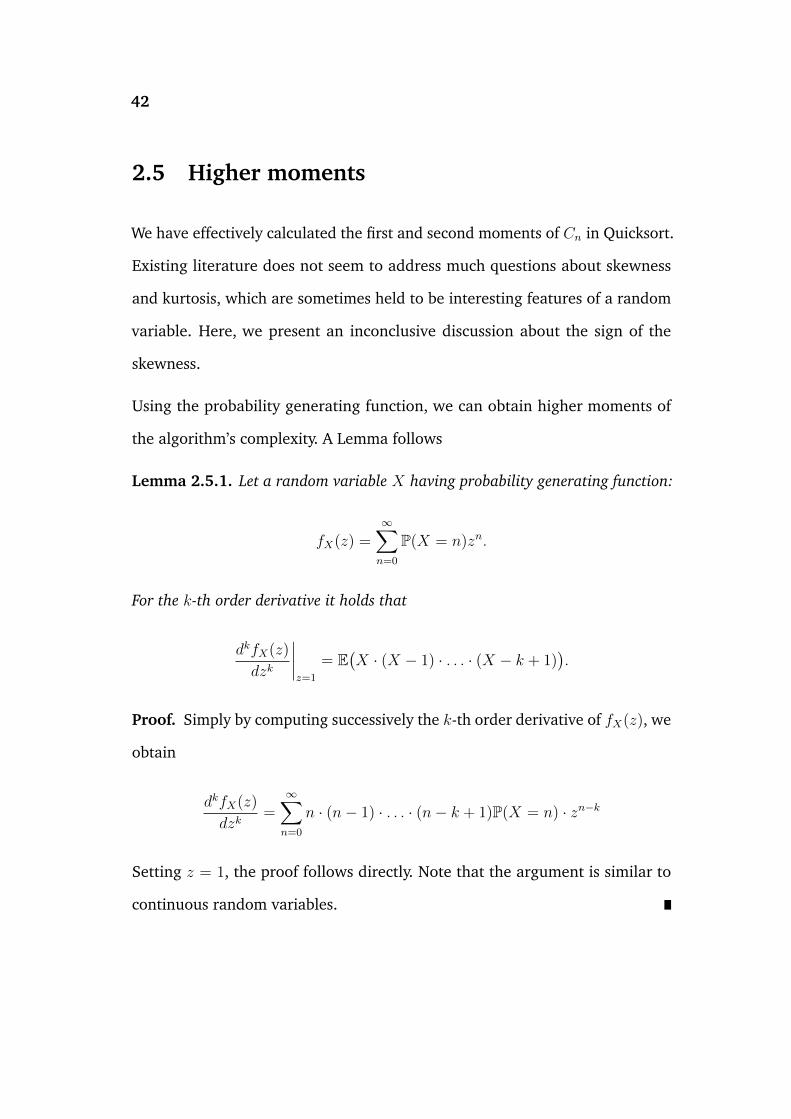
2.5 Higher moments
We have effectively calculated the first and second moments of Cn in Quicksort.
Existing literature does not seem to address much questions about skewness
and kurtosis, which are sometimes held to be interesting features of a random
variable. Here, we present an inconclusive discussion about the sign of the
skewness.
Using the probability generating function, we can obtain higher moments of
the algorithm’s complexity. A Lemma follows
Lemma 2.5.1. Let a random variable X having probability generating function:
fX(z) =∞∑n=0
P(X = n)zn.
For the k-th order derivative it holds that
dkfX(z)
dzk
∣∣∣∣z=1
= E(X · (X − 1) · . . . · (X − k + 1)
).
Proof. Simply by computing successively the k-th order derivative of fX(z), we
obtain
dkfX(z)
dzk=∞∑n=0
n · (n− 1) · . . . · (n− k + 1)P(X = n) · zn−k
Setting z = 1, the proof follows directly. Note that the argument is similar to
continuous random variables.
43
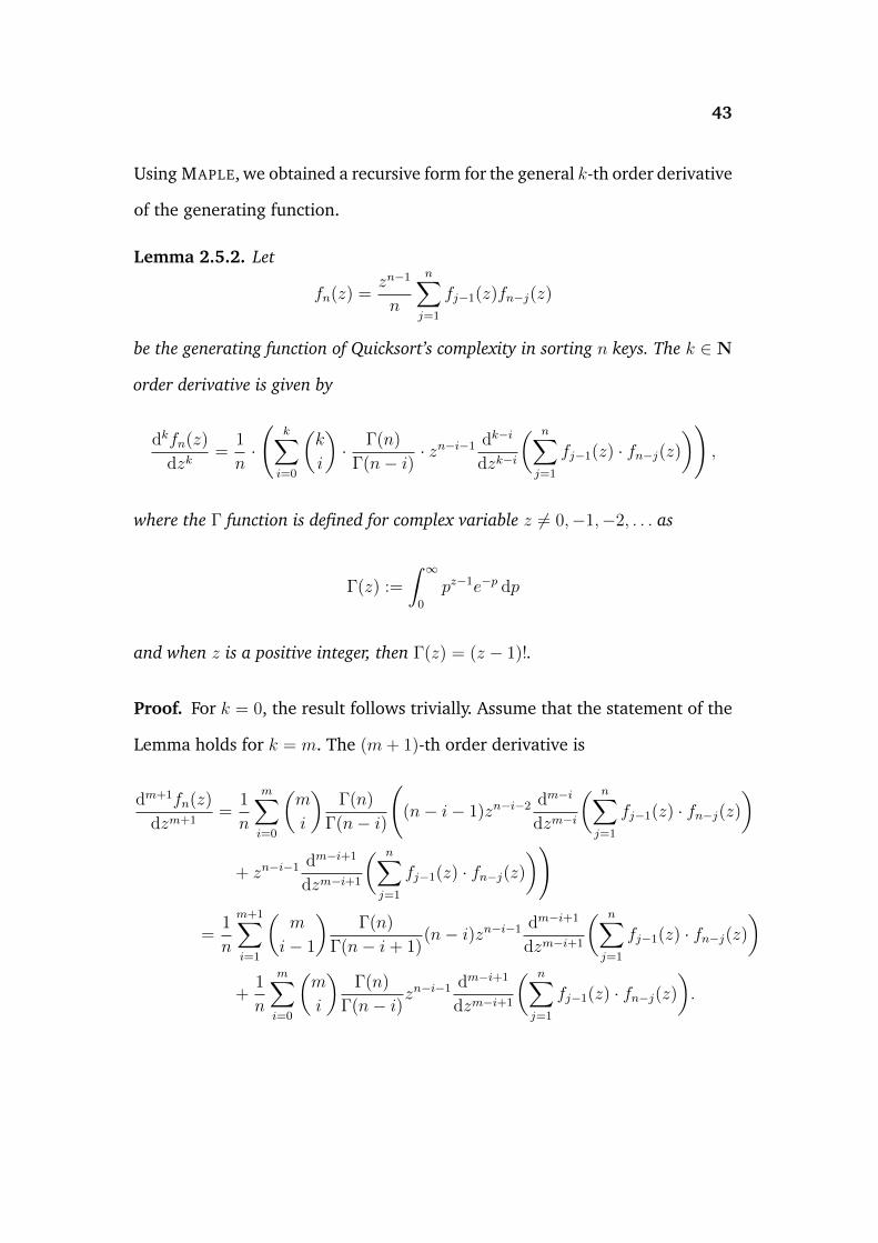
Using MAPLE, we obtained a recursive form for the general k-th order derivative
of the generating function.
Lemma 2.5.2. Let
fn(z) =zn−1
n
n∑j=1
fj−1(z)fn−j(z)
be the generating function of Quicksort’s complexity in sorting n keys. The k ∈ N
order derivative is given by
dkfn(z)
dzk=
1
n·
(k∑i=0
(k
i
)· Γ(n)
Γ(n− i)· zn−i−1 dk−i
dzk−i
( n∑j=1
fj−1(z) · fn−j(z)
)),
where the Γ function is defined for complex variable z 6= 0,−1,−2, . . . as
Γ(z) :=
∫ ∞0
pz−1e−p dp
and when z is a positive integer, then Γ(z) = (z − 1)!.
Proof. For k = 0, the result follows trivially. Assume that the statement of the
Lemma holds for k = m. The (m+ 1)-th order derivative is
dm+1fn(z)
dzm+1=
1
n
m∑i=0
(m
i
)Γ(n)
Γ(n− i)
((n− i− 1)zn−i−2 dm−i
dzm−i
( n∑j=1
fj−1(z) · fn−j(z)
)
+ zn−i−1 dm−i+1
dzm−i+1
( n∑j=1
fj−1(z) · fn−j(z)
))
=1
n
m+1∑i=1
(m
i− 1
)Γ(n)
Γ(n− i+ 1)(n− i)zn−i−1 dm−i+1
dzm−i+1
( n∑j=1
fj−1(z) · fn−j(z)
)
+1
n
m∑i=0
(m
i
)Γ(n)
Γ(n− i)zn−i−1 dm−i+1
dzm−i+1
( n∑j=1
fj−1(z) · fn−j(z)
).
44
Note thatΓ(n)
Γ(n− i+ 1)(n− i) =
Γ(n)
Γ(n− i).
Therefore,
dm+1fn(z)
dzm+1=
1
n
m∑i=1
((m
i− 1
)+
(m
i
))Γ(n)
Γ(n− i)zn−i−1
× dm−i+1
dzm−i+1
( n∑j=1
fj−1(z) · fn−j(z)
).
The well-known identity, (e.g. see [26])
(m
i− 1
)+
(m
i
)=
(m+ 1
i
),
completes the proof.
We should point out that Lemma 2.5.2 is an immediate consequence of Leibniz’s
product rule. Next, we shall ask a Question about the sign of the skewness of
the time complexity of the algorithm, as it is moderately difficult to solve the
recurrence involved, in order to compute the third moment. We already have
seen that the possibility of worst-case performance of the algorithm is rather
small and in the majority of cases the running time is close to the average time
complexity which is O(n log2(n)
). Intuitively, this suggests that the complexity
is negatively skewed. We present the following Question:
Question 2.5.3. Is the skewness S(Cn) of the random number of key comparisons
of Quicksort for the sorting of n ≥ 3 keys negative?
Note that the cases n = 1, 2 are deterministic, since we always make 0 and 1
comparisons for the sorting. This Question may have an affirmative answer,
45
which can be possibly proven by an induction argument on the number of keys.
However, great deal of attention must be exercised to the fact that the random
number of comparisons required to sort the segment of keys less than the
pivot and the segment of keys that are greater than the pivot are conditionally
independent, subject to the choice of pivot.
2.6 Asymptotic analysis
After having examined the number of comparisons of Quicksort, in terms of
average and worst case scenarios, and its variance, it is desirable also to study
the concentration of the random variable Cn about its mean. One might hope,
by analogy with other probabilistic situations, that for large values of n the
number of comparisons is highly likely to be very close to the mean.
The analysis will be confined to the number of comparisons, because this is the
most relevant measure for this thesis. Since our results will be asymptotic in
nature, we need to have some relevant ideas about convergence of sequences
of random variables. The following definitions come from [8], [21].
Definition 2.6.1.
(i) A sequence of random variables X1, X2, . . . is said to converge in distribution
(or converge weakly) to a random variable X if and only if
limn→∞
Fn(x) = F (x)
at every point x where F is continuous. Here Fn(x) and F (x) are respectively the
cumulative distribution functions of random variables Xn and X. We shall denote
46
this type of convergence by XnD−→ X.
(ii) A sequence of random variables X1, X2, . . . is said to converge in probability
to a random variable X if and only if ∀ε > 0 holds
limn→∞
P(|Xn −X| ≥ ε) = 0.
We will denote this type of convergence by XnP−→ X.
(iii) A sequence X1, X2, . . . of random variables is said to converge in Lp-norm
to a random variable X if and only if
limn→∞
E(|Xn −X|p) = 0.
Note that convergence in Lp-norm, for p ≥ 1, implies convergence in probability,
and it is also easy to see that convergence in probability implies convergence in
distribution: see e.g. [8]. Both converse statements are false in general.
We also present the definition of martingale, which shall be employed in a later
stage of our analysis.
Definition 2.6.2. Let Z1, Z2, . . . be a sequence of random variables. We say Zn
is a martingale if and only if
(i) E(|Zn|) <∞, ∀n ∈ N.
(ii) E(Zn|Zn−1, Zn−2, . . . , Z1) = Zn−1.
2.6.1 Binary trees
In this subsection, a central notion to the analysis of Quicksort, and in general
to the analysis of algorithms is discussed. We begin with a definition.

47
Definition 2.6.3. A graph is defined as an ordered pair of two sets (V,E). The set
V corresponds to the set of vertices or nodes. The set E is the set of edges, which
are pairs of distinct vertices.
One kind of graph we concentrate on are trees. A definition of a tree (which
suits us) is as follows [44]:
Definition 2.6.4. Tree is a finite set ∆ of nodes, such that:
(i) There is a unique node called the root of the tree.
(ii) The remaining nodes are partitioned into k ∈ N disjoint sets ∆1,∆2, . . . ,∆k
and each of these sets is a tree. Those trees are called the subtrees of the root.
A particularly common tree is a binary tree. It is defined as a tree with the
property that every node has at most 2 subtrees, i.e. each node – excluding the
root – is adjacent to one parent, so to speak, and up to two offspring, namely left
and right child nodes. Note here that nodes which do not have any child nodes
are called external. Otherwise, they are called internal. The size of a binary tree
is the number of its nodes. The depth of a node is simply the number of edges
from that node to the root in the (unique) shortest path between them and the
height of a binary tree is the length from the deepest node to the root.
An extended binary tree is a binary tree with the property that every internal
node has exactly two offspring [44]. Let Dj be the depth of insertion of a key
in a random binary tree of size j − 1. Since the root node is first inserted to an
empty tree, it holds that D1 := 0. The next inserted key is compared with the
key at the root and if it is smaller, is placed to the left; otherwise is attached as
a right subtree, thus D2 := 1.
48
The internal path length of an extended binary tree having n internal nodes is
defined to be the sum over all internal nodes, of their distances to the root. Let
us denote this quantity by Xn. We then have that
Xn =n∑j=1
Dj.
Similarly, the external path length is defined as the total number of edges in
all the shortest paths from external nodes to the root node. The next Lemma
gives a relationship between those two quantities.
Lemma 2.6.5 (Knuth [44]). For an extended binary tree with n internal nodes
it holds that
Yn = Xn + 2n,
where Yn denotes the external path length of the tree.
Proof. Suppose that we remove the two offspring of an internal node v, with
its offspring being external nodes of the tree. We suppose that v is at distance
h from the root. Then the external path length is reduced by 2(h + 1), as
its two offspring are removed. At the same time, the external path length is
increased by h, because the vertex v has just become an external node. Thus,
the net change is equal to −2(h + 1) + h = −(h + 2). For internal path length
the change is a reduction by −h as v is no longer internal. Thus, overall, the
change in Yn −Xn is equal to −(h + 2) − (−h) = −2. The Lemma follows by
induction.
Binary trees play a fundamental and crucial role in computing and in the analy-
sis of algorithms. They are widely used as data structures, because fast insertion,

49
deletion and searching for a given record can be achieved. In Quicksort, letting
nodes represent keys, the algorithm’s operation can be depicted as a binary
tree. The root node stores the initial pivot element. Since the algorithm at
each recursion splits the initial array into two subarrays and so on, we have an
ordered binary tree. The left child of the root stores the pivot chosen to sort
all keys less than the value of root and the right child node stores the pivot for
sorting the elements greater than the root.
The process continues until the algorithm divides the array into trivial subarrays
having cardinality 0 or 1, which do not need any more sorting. These elements
are stored as external or leaf nodes in this binary structure. It easily follows
that for any given node storing a key k, its left subtree stores keys less than k
and similarly its right subtree contains keys greater than k.
In variants of Quicksort, where many pivots are utilised to partitioning pro-
cess, the generalisation of binary trees provides a framework for the analysis,
though we do not develop this in detail here. In the next subsection, the lim-
iting distribution of the number of comparisons will be analysed, in terms of
trees.
2.6.2 Limiting behaviour
We have previously seen that the operation of the algorithm can effectively
be represented as a binary tree. Internal nodes store pivots selected at each
recursion step of the algorithm: so the root vertex, for example, stores the first
pivot with which all other elements are compared. We are interested in the
total number of comparisons made. To understand this, we note that every
50
vertex is compared with the first pivot which is at level 0 of the tree. The array
is divided into two parts – those above the pivot, and those below it. (Either
of these subarrays may be empty). If a subarray is not empty, a pivot is found
in it and is attached to the root as a child on the left, for the elements smaller
than the first pivot or on the right for the elements larger than the pivot.
The process then continues recursively and each element at level k in the tree
is compared with each of the k elements above it. Thus the total number of
comparisons made is the sum of the depths of all nodes in the tree. This is
equivalent to the internal path length of the extended binary tree. Thus,
Yn = Cn + 2n,
where Yn is the external path length of the tree. To see this, we simply use
Lemma 2.6.5. This fact can be also found in [49].
Generally, assume that we have to sort an array of n distinct items with pivots
uniformly chosen. All n! orderings of keys are equally likely. This is equivalent
to carrying out n successive insertions [46]. Initially, the root node is inserted.
The second key to be inserted is compared with the key at the root. If it is less
than that key, it is attached as its left subtree. Otherwise, it is inserted as the
right subtree. This process continues recursively by a series of comparisons
of keys, until all n keys have been inserted. Traversing the binary search tree
in order, i.e. visiting the nodes of the left subtree, the root and the nodes of
the right subtree, keys are printed in ascending order. Thus, Quicksort can be
explicitly analysed in this way.
51
Recall that each internal node corresponds to the pivot at a given recursion
of the Quicksort process (e.g. the depth of a given node). Thus the first pivot
corresponds to the root node, its descendants or child nodes are pivots chosen
from the two subarrays to be sorted, etc. Eventually, after n insertions, we have
built a binary search tree from top to bottom. We can use this approach to
understand the following Theorem of Régnier [58].
Theorem 2.6.6 (Régnier [58]). Let random variables Yn and Xn denote re-
spectively the external and internal path length of binary search tree, built by n
successive insertions of keys. Then the random variables
Zn =Yn − 2(n+ 1)(Hn+1 − 1)
n+ 1=Xn − 2(n+ 1)Hn + 4n
n+ 1
form a martingale with null expectations. For their variances it holds
Var(Zn) = 7− 2π2
3− 2 loge(n)
n+O
(1
n
).
Proof. By induction on n, the base case being trivial. Suppose we have an
(n−2)-vertex tree and consider the insertion of the (n−1)-th key in the random
binary tree. Its depth of insertion is Dn−1, so that a formerly external node
becomes an internal and we see that its two (new) descendants are both at
depth Dn−1 + 1. Recall that Dn is the random variable counting the depth of
insertion of a key in a random binary tree of size n−1 withD1 := 0 andD2 := 1.
The following equation concerning conditional expectations holds:
nE(Dn|D1, . . . , Dn−1) = (n− 1)E(Dn−1|D1, . . . , Dn−2)−Dn−1 + 2(Dn−1 + 1).
52
This recurrence yields
nE(Dn|D1, . . . , Dn−1)− (n− 1)E(Dn−1|D1, . . . , Dn−2) = Dn−1 + 2.
Summing and using that the left-hand side is a telescopic sum,
nE(Dn|D1, . . . , Dn−1) =n−1∑i=1
(Di + 2) = Yn−1.
The last equation is justified by Lemma 2.6.5. Also, we have
E(Yn|D1, . . . , Dn−1) = E(Yn−1 + 2 +Dn|D1, . . . , Dn−1) =n+ 1
nYn−1 + 2.
Thus, taking expectations and using E(E(U |V )) = E(U),
E(Yn) =n+ 1
nE(Yn−1) + 2⇐⇒ E(Yn)
n+ 1=
E(Yn−1)
n+
2
n+ 1.
This recurrence has solution
E(Yn) = 2(n+ 1)(Hn+1 − 1).
For Zn, we deduce that
E(Zn|D1, . . . , Dn) = E(Yn − E(Yn)
n+ 1|D1, . . . , Dn
)=
2
n+ 1+Yn−1
n− E(Yn)
n+ 1
= Zn−1.
53
Therefore,Zn form a martingale. Further, note that Zn is a linear transformation
of the internal path length Xn, so we get that
Var(Zn) =1
(n+ 1)2· Var(Xn).
Previously, we saw that the number of comparisons is just the internal path
length of a binary search tree. As a reminder the variance of the number of
comparisons is equal to
Var(Cn) = 7n2 − 4(n+ 1)2H(2)n − 2(n+ 1)Hn + 13n.
Hence,
Var(Zn) = 7
(n
n+ 1
)2
− 4H(2)n −
2Hn
n+ 1+
13n
(n+ 1)2.
For the purpose of obtaining the asymptotics of the variance, an important
family of functions, which is called polygamma functions are discussed. The
digamma function is
ψ(z) =d
dzloge Γ(z)
and for complex variable z 6= 0,−1,−2, . . . can be written as [1],
ψ(z) = −γ +∞∑j=0
(1
j + 1− 1
j + z
). (2.7)
In general, ∀k ∈ N, the set
ψ(k)(z) =dk+1
dzk+1loge Γ(z),
54
with ψ(0)(z) = ψ(z), forms the family of polygamma functions. Differentiating
Eq. (2.7),
ψ(1)(z) =∞∑j=0
1
(j + z)2. (2.8)
By Eq. (2.7), it easily follows that
Hn = ψ(n+ 1) + γ.
Further, using the fact that ζ(2) = limn→∞H(2)n =
π2
6[1], where ζ(s) =
∑∞j=1
1
js
is the Riemann zeta function for Re(s) > 1, we obtain
H(2)n +
2Hn
n+ 1=π2
6− ψ(1)(n+ 1) +
2(ψ(n+ 1) + γ)
n+ 1. (2.9)
Eq. (2.9) is asymptotically equivalent to
π2
6+
2 loge(n)
n,
thus, the asymptotic variance is
Var(Zn) = 7− 2π2
3− 2 loge(n)
n+O
(1
n
)= 7− 2π2
3−O
(loge(n)
n
).
Remark 2.6.7. We note that there is a typo in the expression for the asymptotic
variance in Régnier’s paper [58], which is given as
7− 2π2
3+O
(1
n
).

55
The correct formula for the asymptotic variance is stated in Fill and Janson [22].
The key point about martingales is that they converge.
Theorem 2.6.8 (Feller [21]). Let Zn be a martingale, and suppose further that
there is a constant C such that E(Z2n) < C for all n. Then there is a random
variable Z to which Zn converges, with probability 1. Further, E(Zn) = E(Z) for
all n.
We showed that
ZnP−→ Z.
It is important to emphasise that the random variable Z to which we get conver-
gence is not normally distributed. We saw that the total number of comparisons
to sort an array of n ≥ 2 keys, when the pivot is a uniform random variable
on 1, 2, . . . , n is equal to the number of comparisons to sort the subarray of
Un − 1 keys below pivot plus the number of comparisons to sort the subarray
of n − Un elements above pivot plus n − 1 comparisons done to partition the
array. Therefore,
Xn = XUn−1 +X∗n−Un + n− 1,
where the random variables XUn−1 and X∗n−Un are identically distributed and
independent conditional on Un.
Consider the random variables
Yn =Xn − E(Xn)
n.
56
The previous equation can be rewritten in the following form
Yn =XUn−1 +X∗n−Un + n− 1− E(Xn)
n.
By a simple manipulation, it follows that [22], [59]
Yn = YUn−1 ·Un − 1
n+ Y ∗n−Un ·
n− Unn
+ Cn(Un),
where
Cn(j) =n− 1
n+
1
n
(E(Xj−1) + E(X∗n−j)− E(Xn)
).
The random variable Un/n converges to a uniformly distributed variable Ξ on
[0, 1]. A Lemma follows
Lemma 2.6.9. Let Un be a uniformly distributed random variable on 1, 2, . . . , n.
ThenUnn
D−→ Ξ,
where Ξ is uniformly distributed on [0, 1].
Proof. The moment generating function of Un is given by
MUn(s) =n∑k=1
P(Un = k)esk =1
n·
n∑k=1
esk =1
n· e
s(n+1) − es
es − 1.
For the random variable Un/n, it is
MUn/n(s) = MUn(s/n) =1
n·
n∑k=1
esk/n =1
n· e
s(n+1)/n − es/n
es/n − 1.
57
The random variable Ξ has moment generating function
MΞ(s) =
∫ 1
0
est dt =es − 1
s.
Now the moment generating function of Un/n is an approximation to the av-
erage value of esx over the interval [0, 1] and so, as n tends to infinity, we can
replace it by its integral
∫ 1
0
esx dx =
[esx
s
]1
0
=es − 1
s
and now all that is required has been proved.
For the function
Cn(j) =n− 1
n+
1
n·(E(Xj−1) + E(X∗n−j)− E(Xn)
)using the previous Lemma and recalling that asymptotically the expected com-
plexity of Quicksort is 2n loge(n) it follows that
limn→∞
Cn(n · Un/n) = limn→∞
(n− 1
n+
1
n·(E(XUn−1) + E(X∗n−Un)− E(Xn)
))= lim
n→∞
(n− 1
n+
1
n·(
2
(n · Unn− 1
)loge(Un − 1)
+ 2
(n− n · Un
n
)loge(n− Un)− 2n loge(n)
))
= 1 + 2ξ loge ξ + 2(1− ξ) loge(1− ξ) = C(Ξ), ∀ ξ ∈ [0, 1].
58
Thus Cn(n · Un/n) converges to C(Ξ), (see as well in [59]). Therefore, we
obtain
L (Y ) = L(Y · Ξ + Y ∗ · (1− Ξ) + C(Ξ)
).
But this does not work for the normal. Indeed, if Y (and hence Y ∗) are normals
with mean zero and variance σ2, a necessary condition for Y Ξ+Y ∗(1−Ξ)+C(Ξ)
to have mean 0 (which would be needed for the equality to hold) would be
that C(Ξ) = 0. This equality happens with probability equal to 0, as we can
easily deduce. Thus, the distribution which the sequence Yn converges is not
Gaussian.
2.6.3 Deviations of Quicksort
It is desirable to derive bounds on the deviation of the random number of
pairwise comparisons, needed to sort an array of n distinct elements from its
expected value, as n gets arbitrarily large. We remind ourselves that the pivot
is uniformly chosen at random.
We shall derive bounds on the following probability
P(∣∣∣∣ Cn
E(Cn)− 1
∣∣∣∣ > ε
)
for ε > 0, sufficiently small. From Chebyshev’s inequality, we obtain a bound
for the above probability. Chebyshev’s inequality is as follows [21]:
59
Theorem 2.6.10 (Chebyshev’s inequality). Let X be a random variable, with
E(X2) <∞. Then, for any real number a > 0
P(|X| ≥ a
)≤ E(X2)
a2.
If E(X) = m and Var(X) = σ2, then
P(|X −m| ≥ a
)≤ σ2
a2.
The random variable Yn =Cn
E(Cn)has mean and variance,
E(Yn) = E(
CnE(Cn)
)=
1
E(Cn)· E(Cn) = 1
Var(Yn) = Var
(Cn
E(Cn)
)=
1
E2(Cn)· Var(Cn)
=−4(n+ 1)2H
(2)n − 2(n+ 1)Hn + (7n+ 13)n(2(n+ 1)Hn − 4n
)2 .
For ε > 0, we have
P(|Yn − 1| > ε) <Var(Yn)
ε2=−4(n+ 1)2H
(2)n − 2(n+ 1)Hn + (7n+ 13)n
ε2(2(n+ 1)Hn − 4n
)2 .
It holds that,
Var(Cn) = −4(n+ 1)2H(2)n − 2(n+ 1)Hn + (7n+ 13)n
≤ 7n2 + 13n
≤ 20n2,
60
using that the other terms are negative and n ≥ 1. Further, using that
limn→∞
H(2)n =
∞∑n=1
1
n2=π2
6,
we get
Var(Cn) = −4(n+ 1)2H(2)n − 2(n+ 1)Hn + (7n+ 13)n
≥ (7n+ 13)n− 4(n+ 1)2π2/6− 2(n+ 1)(loge(n) + γ + o(1)
)= (7− 2π2/3)n2
(1 + o(1)
).
From above inequalities, we deduce that Var(Cn) = Θ(n2). Thus,
P(|Yn − 1| > ε) <Var(Yn)
ε2=
Θ(n2)
ε2(2(n+ 1)Hn − 4n
)2 = O((ε loge(n))−2
).
Rösler [59] derived a sharper bound. He showed that this probability is O(n−k),
for fixed k. McDiarmid and Hayward [50] have further sharpened the bound.
Their Theorem is
Theorem 2.6.11 (McDiarmid and Hayward [50], McDiarmid [51]).
Let ε = ε(n) satisfy1
loge(n)< ε ≤ 1. Then as n→∞,
P(|Yn − 1| > ε) = n−2ε(
log(2)e (n)−loge(1/ε)+O(log
(3)e (n))
),
where log(k+1)e (n) := loge
(log(k)
e (n))
and log(1)e (n) = loge(n).
In the recent paper of McDiarmid [51], Theorem 2.6.11 is revisited using con-
centration arguments. By this result, it can be easily deduced, that Quicksort
with good pivot choices performs well, with negligible perturbations from its
61
expected number of comparisons. As we previously saw, Quicksort can be de-
picted as an ordered binary tree. The root node or node 1 corresponds to the
input array of length L1 = n to be sorted.
A pivot with rank Un = 1, 2, . . . , n is selected uniformly at random and the
initial array is divided into two subarrays, one with elements less than the pivot
and a second, with elements greater than the pivot. Then, the node at the left
corresponds to the subarray of keys that are less than the pivot, with length
L2 = Un − 1 and the node at the right corresponds to the subarray of keys that
are greater than the pivot, with length L3 = n− Un.
Recursively, Quicksort runs on these two subarrays and split them in four subar-
rays, until we get trivial subarrays and the initial array is sorted. For j = 1, 2 . . .
let Lj be the length of the array to be sorted at j node and Mnk be the maximum
cardinality of the 2k subarrays, after k recursions of Quicksort. It is [50],
Mnk = maxL2k+i : i = 0, 1, . . . , 2k − 1.
The following Lemma gives an upper bound for the probability that the maxi-
mum length of 2k subarrays Mnk , will exceed α times the initial set’s length n.
We easily see that the upper bound is rather small quantity. Thus, we deduce
that the length of the array is rapidly decreasing, as Quicksort runs.
Lemma 2.6.12 (McDiarmid and Hayward [50], McDiarmid [51]).
For any 0 < α < 1 and any integer k ≥ loge
(1
a
)it holds
P (Mnk ≥ αn) ≤ α
(2e · loge(1/α)
k
)k.
62
So far, the analysis explicitly assumed the presence of distinct numbers. How-
ever, in many sorting problems, one can come across with duplicates. As we
will see next, we have to consider the presence of equal numbers and how this
affects the algorithm’s performance.
2.7 Quicksorting arrays with repeated elements
In this section, we consider the presence of equal keys. In some cases, there
may be multiple occurrences of some of the keys – so that there is a multiset
of keys to be sorted. If a key ai appears si times, we call si the multiplicity of
ai.
Thus, we have a multiset of the array s1 · a1, s2 · a2, . . . , sn · an, with s1 + s2 +
. . . + sn = N and n is the number of distinct keys. Without loss of generality,
we assume that we have to sort a random permutation of the array s1 · 1, s2 ·
2, . . . , sn · n. Obviously, when s1 = s2 = . . . = sn = 1, then the array contains
n = N distinct keys.
Consider an array consisting of keys with “large” multiplicities. The usual Quick-
sort algorithm is quite likely to perform badly, since keys equal to the pivot are
not being exchanged. Recall that Hoare’s partitioning routine [30] described
in the previous Chapter, utilises two pointers that scan for keys greater than
and less than the pivot, so at the end of partition, keys equal to pivot may
be on either or both subarrays, leading to unbalanced partitioning which we
saw is usually undesirable. The algorithm can be further tweaked for efficient
sorting of duplicates, using a ternary partition scheme [7]. Keys less than pivot
63
are on left, keys equal to pivot on middle and on right, keys greater than the
pivot.
Hoare’s partitioning scheme can be easily modified, in order for the pointers to
stop on equal keys with the pivot. In other words, the lower pointer searches
for a key greater than or equal to the pivot and the upper one for a key smaller
than or equal to the pivot. Sedgewick [64] considers a partitioning routine,
where only one of the pointers stops on keys either greater or smaller than the
pivot.
The recurrence for the expected number of key comparisons E(C(s1, s2, . . . , sn)
)is
E(C(s1, s2, . . . , sn)
)= N − 1 +
1
N
n∑i=1
si
(E(C(s1, . . . , si−1)
)+ E
(C(si+1, . . . , sn)
)).
The analysis has been done in [64]. The solution of the recurrence is
E(C(s1, s2, . . . , sn)
)= 2
(1 +
1
n
)NHn − 3N − n. (2.10)
Note that when n = N , i.e. the keys to be sorted are distinct, Eq. (2.10) yields
the expected number of comparisons, when the array is partitioned using n− 1
comparisons. As we saw in the previous Chapter, a different partitioning scheme
proposed and analysed in [46], [63], utilises N+1 comparisons for partitioning
an array of N keys. In this case, an upper bound for large n to the expected
number of comparisons is [64],
E(C(s1, s2, . . . , sn)
)= 2N(HN + 1)− 2 +O
(N2
n
).
Chapter 3
Sorting by sampling
The preceding analysis has shown that Quicksort is prone to poor performance,
when the chosen pivots happen to be (close to) the smallest or greatest keys
in the array to be sorted. The partitioning yields trivial subarrays, leading to
quadratic running time taken by the algorithm, and increasing the chances of
‘crashing’, i.e. an application of Quicksort may terminate unsuccessfully through
running out of memory. On the other hand, good choices of pivot yield a much
more efficient algorithm. The uniform model suggests that in fact any key has
equal probability to be selected as pivot. In this Chapter, we discuss and analyse
the general idea of how one can increase the probability that the selected pivots
will produce (reasonably) balanced partitions, by trying to ensure that their
ranks are ‘near’ the middle of the array.
A naive idea towards this, would be finding the median of the keys and use this
as pivot. However, it is obvious that the finding of median imposes additional
costs to the algorithm. Therefore, despite the always good choices, this method
might not be better than choosing the pivot randomly. Instead of finding the
median of the array to be sorted, it might be more efficient to randomly pick a
64
65
sample from the array, find its median and use this as pivot. In what it follows,
we will analyse this idea and its variants.
3.1 Median of (2k+1) partitioning
Singleton [68] suggested to randomly select three keys from the array to be
sorted and use their median as pivot, leading to a better estimate of the median
of the array and reducing further the chances of worst case occurrence.
This modification can be generalised as to choosing a sample of (2k+1) keys at
every recursive stage, computing their median and using that median as pivot,
partitioning n > 2k + 1 keys. Arrays that contain at most (2k + 1) keys are
sorted by a simpler algorithm, such as insertion sort. The cost of sorting these
small arrays is linear with respect to n.
Letting Cn2k+1 denote the number of comparisons required to sort n keys
when the pivot is the median of a random sample of (2k+1) elements, uniformly
selected from the relevant array, the recurrence for the average number of
comparisons is given by (see [46])
E(Cn2k+1) = n+ 1 +2(n
2k + 1
) n∑j=1
(j − 1
k
)(n− jk
)E(Cj−12k+1).
Multiplying both sides by(
n
2k + 1
),
(n
2k + 1
)E(Cn2k+1) =
(n
2k + 1
)(n+ 1) + 2
n∑j=1
(j − 1
k
)(n− jk
)E(Cj−12k+1).
66
Multiplying by zn and summing over n, in order to obtain the generating func-
tion for the expected number of comparisons, f(z) =∑∞
n=0 E(Cn2k+1)zn
∞∑n=0
(n
2k + 1
)E(Cn2k+1)z
n =
∞∑n=0
(n
2k + 1
)(n+ 1)zn + 2
∞∑n=0
n∑j=1
(j − 1
k
)(n− jk
)E(Cj−12k+1)z
n.
(3.1)
It holds
∞∑n=0
(n
2k + 1
)E(Cn2k+1)z
n =1
(2k + 1)!
∞∑n=0
n(n− 1) . . . (n− 2k)E(Cn2k+1)zn
=z2k+1f (2k+1)(z)
(2k + 1)!,
where f (2k+1)(z) denotes the (2k + 1)-th order derivative of f(z). For the first
sum in the right-hand side of Eq. (3.1)
∞∑n=0
(n
2k + 1
)(n+ 1)zn =
z2k+1
(2k + 1)!
( ∞∑n=0
zn+1
)(2k+2)
=z2k+1
(2k + 1)!
(z
1− z
)(2k+2)
.
The (2k + 2)-th order derivative of(z/(1− z)
)can be easily seen by induction
that is equal to(2k + 2)!
(1− z)2k+3.
67
Expanding out the double sum of Eq. (3.1),
∞∑n=0
n∑j=1
(j − 1
k
)(n− jk
)E(Cj−12k+1)z
n =
(0
k
)(0
k
)E(C02k+1)z+((
0
k
)(1
k
)E(C02k+1) +
(1
k
)(0
k
)E(C12k+1)
)z2+((
0
k
)(2
k
)E(C02k+1) +
(1
k
)(1
k
)E(C12k+1) +
(2
k
)(0
k
)E(C22k+1)
)z3 + . . .
=
((0
k
)E(C02k+1) +
(1
k
)E(C12k+1)z + . . .
)((0
k
)z +
(1
k
)z2 + . . .
)
=
(∞∑n=0
(n
k
)E(Cn2k+1)z
n
)(∞∑n=0
(n
k
)zn+1
)
=zkf (k)(z)
k!· z
k+1
k!
( ∞∑n=0
zn)(k)
=z2k+1f (k)(z)
k!(1− z)k+1.
The recurrence is transformed to the following differential equation
z2k+1f (2k+1)(z)
(2k + 1)!=
(2k + 2)z2k+1
(1− z)2k+3+
2z2k+1f (k)(z)
k!(1− z)k+1.
Multiplying both sides by(
1− zz
)2k+1
,
(1− z)2k+1f (2k+1)(z)
(2k + 1)!=
2(k + 1)
(1− z)2+
2(1− z)kf (k)(z)
k!,
which is a Cauchy–Euler differential equation. This type of differential equa-
tions arises naturally to the analysis of searching–sorting algorithms and urn
models [14]. Substituting x = 1− z, and putting h(x) = f(1− x), we get
(−1)2k+1x2k+1h(2k+1)(x)
(2k + 1)!=
2(k + 1)
x2+
2(−1)kxkh(k)(x)
k!.
68
We use the differential operator Θ for the solution of the differential equation.
It is defined by
Θ(h(x)
):= xh′(x)
and by induction
(Θ
k
)h(x) =
xkh(k)(x)
k!.
Applying the operator, our equation becomes
P2k+1(Θ)h(x) =2(k + 1)
x2,
where the indicial polynomial is equal to
P2k+1(Θ) = (−1)2k+1
(Θ
2k + 1
)− 2(−1)k
(Θ
k
).
We proceed to identify the nature of the roots of the polynomial. A Lemma
follows:
Lemma 3.1.1. The indicial polynomial P2k+1(Θ) has 2k + 1 simple roots, with
real parts greater than or equal to −2. The real roots are 0, 1, . . . , k − 1; −2;
3k + 2, if k is odd and the 2⌊k2
⌋complex roots ρ1, . . . , ρb k2c with their conjugates
ρ1, . . . , ρb k2c.
Proof. Let α = x+ iy being a root of the polynomial. Then
(α
2k + 1
)= −2(−1)k
(α
k
). (3.2)
69
From Eq. (3.2), we deduce that k real roots of the polynomial P2k+1(Θ) are
0, 1, . . . , k − 1. For α 6= 0, 1, . . . , k − 1, we have that
(α− k)
(k + 1)· (α− k − 1)
(k + 2)· . . . · (α− 2k)
(2k + 1)= −2(−1)k. (3.3)
Suppose that Re(α) < −2. Then
∣∣∣∣α− kk + 1
∣∣∣∣ =
√(x− k)2 + y2
k + 1>
√(−(k + 2)
)2+ y2
k + 1≥ k + 2
k + 1.
∣∣∣∣α− k − 1
k + 2
∣∣∣∣ =
√(x− k − 1)2 + y2
k + 2>
√(−(k + 3)
)2+ y2
k + 2≥ k + 3
k + 2.
...∣∣∣∣α− 2k
2k + 1
∣∣∣∣ =
√(x− 2k)2 + y2
2k + 1>
√(−2(k + 1)
)2+ y2
2k + 1≥ 2k + 2
2k + 1,
so the product of the moduli in Eq. (3.3) is greater than or equal to the telescop-
ing product (2k + 2)/(k + 1) = 2, arriving in contradiction. Thus, for any root
α of the polynomial, it is proved that Re(α) > −2. Moreover, this argument
shows that −2 is the unique root with real part equal to −2. To see all roots
are simple, assume that there does exist a repeated root α. Differentiating the
polynomial,
P ′2k+1(Θ) = −(
Θ
2k + 1
) 2k∑j=0
1
Θ− j− 2(−1)k
(Θ
k
) k−1∑j=0
1
Θ− j
and
(α
2k + 1
) 2k∑j=0
1
α− j= −2(−1)k
(α
k
) k−1∑j=0
1
α− j. (3.4)
70
Eq. (3.2) and (3.4) imply that for a repeated root must hold
2k∑j=0
1
α− j=
k−1∑j=0
1
α− j
or2k∑j=k
1
α− j= 0. (3.5)
Consequently, Eq. (3.5) implies that Im(α) = 0 and α ∈ (k, k + 1) ∪ (k + 1, k +
2) ∪ . . . ∪ (2k − 1, 2k). Considering Eq. (3.2), the left-hand side has modulus
less than 1, since k < α < 2k+ 1. However, the right-hand side of Eq. (3.2) has
modulus greater than 2, leading to contradiction.
Since the roots are simple, we can factor our polynomial in the form
(Θ− r1)(Θ− r2) . . . (Θ− r2k)(Θ + 2)h(x) =2k + 2
x2.
The solution to the differential equation (Θ− a)h(x) = xb is [63],
h(x) =
xb
b− a+ cxa, if a 6= b
xb loge(x) + cxa, if a = b.
Therefore, applying (2k + 1) times the solution, we obtain
h(x) =2k + 2
(−2− r1)(−2− r2) . . . (−2− r2k)
loge(x)
x2+
2k+1∑j=1
cjxrj ,
71
where cj are the constants of integration. Note that
P2k+1(Θ) = (Θ + 2)S2k(Θ),
thus, the expression in the denominator S2k(−2) is
S2k(−2) = P ′2k+1(−2)
= −(−2
2k + 1
) 2k∑j=0
1
−2− j− 2(−1)k
(−2
k
) k−1∑j=0
1
−2− j
= −(2k + 2)(H2k+2 −Hk+1).
Reverting to the previous notation,
f(z) = − 1
H2k+2 −Hk+1
loge(1− z)
(1− z)2+
2k+1∑j=1
cj(1− z)rj .
Using the identity [26],
1
(1− z)m+1loge
(1
1− z
)=∞∑n=0
(Hn+m −Hm
)(n+m
m
)zn
and the binomial Theorem, the solution of the differential equation can be
written in terms of series,
f(z) =1
H2k+2 −Hk+1
∞∑n=0
((n+ 1)Hn − n
)zn +
∞∑n=0
2k+1∑j=1
cj(−1)n(rjn
)zn.
72
Extracting the coefficients, the expected number of comparisons of ‘median of
(2k + 1)’ Quicksort is
E(Cn2k+1) =1
H2k+2 −Hk+1
((n+ 1)Hn − n
)+
2k+1∑j=1
(−1)nRe
(cj
(rjn
)).
The real roots of the polynomial 0, 1, . . . , (k − 1) do not contribute to the ex-
pected number of comparisons, since n > 2k + 1 and when k is odd, the root
(3k + 2) adds a negligible constant contribution. Further, note that the root
r2k+1 = −2, contributes c2k+1(n+ 1), with c2k+1 ∈ R. Therefore
E(Cn2k+1) =1
H2k+2 −Hk+1
((n+ 1)Hn − n
)+ c2k+1(n+ 1)
+ 2
b k2c∑j=1
(−1)nRe
(cj
(ρjn
))+O(1).
The asymptotics of the real parts in the last sum is given in [27]. It is proved
that
2(−1)nRe
(cj
(ρjn
))= O(n−(Re(ρj)+1))
and asymptotically the expected number of key comparisons is
E(Cn2k+1) =1
H2k+2 −Hk+1
n loge(n) +
(c2k+1 +
1
H2k+2 −Hk+1
(γ − 1
))n
+ o(n),
since all the other roots have real parts greater than −2. The solution contains
the case of ordinary Quicksort, where the pivot is randomly selected and of
‘median of 3’ Quicksort. The coefficient of the leading term in the latter case
73
is1
H4 −H2
=12
7,
thus the expected number of key comparisons is
E(Cn3) =12
7(n+ 1)Hn +O(n).
van Emden [19] obtained the asymptotic cost of the expected number of com-
parisons, using entropy arguments. The leading term is equal to
an log2(n),
where
a =1
E(H)= − 1
2
∫ 1
0
xg(x) log2(x) dx
.
Here g(x) denotes the probability density of the median of a random sample
of (2k + 1) elements and E(H) is the expected information yielded from a
comparison. The nice and simple asymptotic form for the mean number of
comparisons is
E(Cn2k+1) ∼loge(2)
H2k+2 −Hk+1
n log2(n).
Note that this result, yields the expected number of comparisons of standard
Quicksort, for k = 0. In this case,
a = 2 loge 2,
74
thus
E(Cn) ∼ 1.386n log2(n).
The notion of entropy is of great importance to the analysis presented in this
thesis. Entropy is a measure of uncertainty regarding the events of a random
variable. In other words, a higher uncertainty about the outcome of a random
variable pertains to increased entropy. In the trivial case, where the probability
of occurrence of an event is 1, the entropy is equal to 0, as there is no uncertainty.
A formal definition follows [65].
Definition 3.1.2. The Shannon’s entropy H of a discrete random variable X
taking the values x1, x2, . . . , xn with probabilities p(x1), p(x2), . . . , p(xn) is defined
by,
H(X) = −n∑i=1
p(xi) logb(p(xi)
).
The base b of the logarithm will be normally equal to two; in this case we mea-
sure bits of entropy. We should mention that the notationH(X) does not merely
denote a function of X; entropy is a function of the probability distribution.
Generally, in sorting algorithms that utilise comparisons for this task, entropy
quantifies the amount of information gained from the sorting. Consider an un-
sorted array, with all the n! permutations equally likely. A comparison gives 1
bit of information, thus at least log2(n!) = Ω(n log2(n)
)comparisons are needed
for a complete sort – see in [5]. This quantity is called information–theoretic
lower bound. The range of entropy is given in the following Lemma.
75
Lemma 3.1.3.
0 ≤ H(X) ≤ logb(n).
Proof. Since logb p(xi) ≤ 0, the left inequality follows immediately. Noting that
the logarithm is concave function and applying Jensen’s inequality [38], which
for a random variable X and a concave function f , states that
f(E(X)
)≥ E
(f(X)
),
we have
n∑i=1
p(xi) logb
(1
p(xi)
)≤ logb
(n∑i=1
p(x1)1
p(xi)
)
= logb(n).
The next four definitions can be found in [16], [53] and [65].
Definition 3.1.4. The joint entropy H(X, Y ) of two discrete random variables X
and Y is defined as
H(X, Y ) = −∑x∈X
∑y∈Y
p(x, y) logb p(x, y),
where p(x, y) is the probability that X takes the value x and Y the value y.
76
Definition 3.1.5. The conditional entropy H(X|Y ) of two discrete random vari-
ables X and Y is defined as
H(X|Y ) = −∑x∈X
∑y∈Y
p(x, y) logbp(x, y)
p(y).
Definition 3.1.6. The information content of a random variable X, with proba-
bility distribution P(X) is
I(X) = − logb P(X).
From definition 3.1.6, one can easily deduce, that
H(X) = E(I(X)
).
In other words, entropy is the expected value of the information. We proceed
to the definition of mutual information.
Definition 3.1.7. The mutual information of two discrete random variables X
and Y is defined as:
I(X ∧ Y ) =∑x∈X
∑y∈Y
p(x, y) logbp(x, y)
p(x)p(y)= H(X)−H(X|Y )
and quantifies the amount of information provided about X by Y .
These definitions will be used in a later part of the thesis.
We have to point out that up until now, our analysis did not take into account
the added overhead of finding the median at each stage. In the simple case
77
of three elements, the overhead is not significant, but for larger samples this
might have adversary effects to the efficiency of Quicksort.
For the selection of the median, we use Hoare’s Find algorithm [29] or Quick-
select. This simple and intuitive algorithm searches for an element of a given
rank m in an array of n keys. As in Quicksort, one partitions the array around
a randomly chosen pivot, which at the end of the partition process is moved to
its final position, j. If m = j, the pivot is the sought element and the search is
completed. Otherwise, if m < j, Quickselect is recursively invoked to the left
subarray of j − 1 keys. Conversely, if m > j, we search in the right subarray for
the element of rank (m− j).
Quickselect is ideal in situations where we want to identify order statistics,
without the need to do a complete sort. The average number of comparisons
E(Cn;m) required for the retrieval of the m-th order statistic in an array of n
keys, is given by [46]
E(Cn;m) = 2(n+ 3 + (n+ 1)Hn − (m+ 2)Hm − (n−m+ 3)Hn+1−m
).
For the sample of (2k+1) keys, the rank of the median is k+1. Therefore,
E(C2k+1;k+1) = 2(2k + 4 + (2k + 2)H2k+1 − 2(k + 3)Hk+1
).
The cost for finding the median of a random sample of 3 keys is 8/3 com-
parisons at each stage. However, as the sample of keys increases, in order to
obtain a more accurate estimate of the median, the added overhead imposes a
bottleneck to the efficiency of the algorithm.
78
The computation of other measures of this variant, such as the expected number
of exchanges and passes can be performed by solving analogous recurrences,
as the one for the number of comparisons. The average number of passes is
recursively given by
E(Pn2k+1) = 1 +2(n
2k + 1
) n∑j=1
(j − 1
k
)(n− jk
)E(Pj−12k+1),
where the “toll function” is now one recursive call to the algorithm, after the
chosen pivot is the median of (2k + 1) keys, which yields two subarrays. This
recurrence can be turned to a differential equation with solution
E(Pn2k+1) =n+ 1
2(H2k+2 −Hk+1)− 1,
noting that for k = 0, the average number of passes is n. In the scheme, where
arrays containing m or fewer keys are sorted by insertion sort, the average costs
are reduced. We refer to [27] where this variant is analysed.
3.2 Remedian Quicksort
In the previous section, we analysed the modification of Quicksort, where the
pivot is selected as the median of a sample of (2k + 1) elements. This variant
offers better protection against the occurrence of trivial partitions. However,
there are some cases, where the running time of this partitioning scheme can
go quadratic. Consider the application of ‘median of 3’ Quicksort in an array of
n numbers, where the keys at positions 1, n and⌊n+1
2
⌋are selected as elements
of the sample. In case that two keys of this sample happen to be the smallest

79
(or greatest) elements of the array, the chosen pivot will be 2 (or n−1), leading
to trivial partitioning, making Quicksort everything else, except quick! In [63],
a permutation of the array 1, . . . , 15 is given, which leads Quicksort to worst-
case performance and in [20], an algorithm is presented which forms the worst-
case permutation.
In order to remedy this, a bigger sample of (2k+ 1)β keys is randomly selected,
its remedian is found and used as partitioning element of the array to be
sorted. The remedian of the sample is recursively defined to be the median of
(2k + 1) remedians of (2k + 1)β−1 elements, where the remedian of (2k + 1)
elements is the median, and is shown to be a robust estimator of the median
[60], [72].
A particular case of the remedian Quicksort widely used in sorting applications
is Tukey’s ‘ninther’, where the selected pivot is the median of three medians
of three samples, each containing three elements [14], [72]. In practical im-
plementations, this variant exhibits faster running time [7] with little added
overhead. Specifically, the computation of the remedian of 9 elements takes
on average 4× 83
comparisons at each call – four times more than finding the
median of 3 randomly chosen keys.
Let Cn(2k+1)β denote the number of comparisons required for the complete
sorting of an array of n distinct keys, where the chosen pivot at each call is the
remedian of a random sample of (2k + 1)β elements. The recurrence relation
is much more complicated than the previous ones and the probability pβj that
80
the remedian of (2k + 1)β elements is the (j + 1)-th element is
pβj = (2k + 1)!∑
α1+...+α2k+1=j
p(α1, . . . , α2k+1)
(j
α1,...,α2k+1
)((2k+1)β−j−1
(2k+1)β−1−1−α1,...,(2k+1)β−1−α2k+1
)((2k+1)β
(2k+1)β−1,...,(2k+1)β−1
) ,
where (j
α1, . . . , α2k+1
)=
j!
α1! . . . α2k+1!
is the multinomial coefficient and p(α1, . . . , α2k+1) is defined by
p(α1, . . . , α2k+1) = p(β−1)α1
(p(β−1)0 + . . .+ p
(β−1)α2−1 ) · . . . · (p(β−1)
α2k+1+ . . .+ p
(β−1)
(2k+1)β−1),
with p(0) = 1. See as well [14], where the ‘splitting’ probabilities of 3d remedian
are presented.
Bentley’s and McIlroy’s experiments on the ‘remedian of 32’ Quicksort [7]
showed that the average number of key comparisons is 1.094n log2(n)− 0.74n,
very close to the information–theoretic lower bound of n log2(n)− 1.44n. This
Quicksort utilises the ‘ninther’ partitioning for large arrays, then the ‘median of
3’ is used and as the algorithm proceeds, the partitioning strategy changes to
the standard uniform pivot selection. The paper written by Durand [18] con-
firmed these experimental results, where the average number of comparisons
is being given by
E(Cn32) = 1.5697n loge(n)− 1.0363n+ 1.5697 loge(n)− 7.3484 +O
(1
n
).
From a theoretical point of view, this variant yields savings on the expected time
needed for the sorting, with little additional cost of computing the remedian.
However, the recurrences are quite involved, as the remedian has an inherent
81
recursive definition. A different approach would be to randomly choose a larger
sample and use its elements as pivots through complete sorting. An obvious
advantage of this method, is that the cost of computing the median or remedian
of a sample at each call of the algorithm is avoided and instead all the pivots
for the subsequent calls belong in one sample.
3.3 Samplesort
Having examined the strategy of selecting the median of a sample as pivot and
the more complicated ‘remedian’ variant, we proceed to the analysis of Sam-
plesort algorithm invented by Frazer and McKellar [24]. Instead to randomly
select a sample of keys at each stage, computing the median and using it as
pivot, a larger sample of 2k − 1 keys is selected and extracted out of the array.
It is sorted and its keys are being used as partitioning elements for the sorting
of the array.
First the median of the sample is used as pivot, then the lower quartile to
the lower subarray and the upper one to the subarray of the elements that are
greater than the median. When the sample is exhausted, the resulting subarrays
can be recursively sorted by the same procedure or by standard Quicksort.
For convenience, let 2t + 1 = 2k − 1 and let us denote the total number of
comparisons of Samplesort applied to n keys by C2k−1
n . Then, C2k−1
n is equal
to the number of comparisons to sort the sample of 2k − 1 elements, plus the
number of comparisons to insert its elements to the remainder of the array, plus
the number of comparisons required to sort the resulting 2k subarrays, using
ordinary Quicksort [24]. For the sorting of the sample, we use Quicksort and
82
the average number of comparisons is
2(2t+ 2)H2t+1 − 4(2t+ 1). (3.6)
Assume that the sorted sample is x1 < x2 < . . . < xt+1 < . . . < x2t+1. First,
the median xt+1 is inserted to its final position in the array of n − 2t keys, by
pairwise comparisons of the n− 2t− 1 keys to xt+1. The cost of partitioning is
n − 2t − 1 comparisons. Then, the first quartile is inserted to the subarray of
the elements less than the median xt+1 and the third quartile to the subarray
of the elements greater than xt+1. The cost of partitioning these two subarrays
is n− 2t− 1 comparisons, since the sum of their lengths is n− 2t− 1 keys. The
process is continued until all the elements of the sample are used as pivots and
this will take 2t+ 1 partitioning stages. Thus, an approximation to the average
number of comparisons for the insertion of the sample is [24], [49],
(n− 2t− 1) log2(2t+ 1). (3.7)
After all elements have been inserted, there are 2(t+ 1) subarrays to be sorted
by Quicksort. The expected number of comparisons is [24]
2(n+ 1)(Hn+1 −H2(t+1))− 2(n− 2t− 1). (3.8)
83
Putting together Eq. (3.6), (3.7) and (3.8), we have that the expected number
of comparisons of Samplesort is
2(n+ 1)(Hn+1 −H2(t+1))− 2(n− 2t− 1) + (n− 2t− 1) log2(2t+ 1)
+ 2(2t+ 2)H2t+1 − 4(2t+ 1). (3.9)
For large values of n, the expected number of comparisons is given by the
following Corollary.
Corollary 3.3.1 (Frazer and McKellar [24]). The asymptotic expected number
of comparisons taken by Samplesort for the sorting of an array of n keys, using a
randomly chosen sample of l keys, is
E(Cln ) = 1.386n log2(n)− 0.386(n− l
)log2(l)− 2n− 0.846l.
It is worthwhile to note that the programming of Samplesort is simple and
straightforward, thus making it a suitable candidate to sorting applications. It
is proven in [24], that the procedure is asymptotically optimal, i.e. as n→∞,
the expected number of comparisons approaches the information–theoretic
bound. The process of randomly drawing the sample out of the array to be
samplesorted should be carefully selected, to the effect that the elements of the
sample will produce ‘balanced’ partitions. The main feature of Samplesort is
that partitioning preserves the order of the sample, thus its keys are exchanged
with the ones that they have to, so as to the exhaustion of the sample, its
elements to be spread far apart.
84
In the direction of choosing a more ‘centered’ sample, one can proceed by
randomly selecting three samples – each containing three keys – and computing
their medians, at an extra cost of 8 comparisons. For the sorting of larger
arrays, the number of samples will obviously be greater. The medians will be
used as elements of the sample and the remaining elements can be randomly
chosen from the array. It should be noted, that this is an initial idea, lacking
the mathematical analysis.
Albacea [2] derived a modification of Samplesort. This variant starts with 1
key, that is used as pivot for the partition of 2 keys, so to have a sorted array
of 3 keys. These keys are used as pivots for the partitioning of 4 keys, so as to
obtain a sorted array of 7 keys and so on, until the whole array is sorted. It is
proven [2] that the estimated expected number of key comparisons is
ndlog2(n+ 1)e − 2dlog2(n+1)e − n+ dlog2(n+ 1)e+ 1.
The derivation of the expected number of comparisons remains an open prob-
lem.
Chapter 4
Sorting by multiple pivots
In this Chapter, different partitioning routines are analysed. These schemes
utilise many pivots for the partitioning of the array and naturally arise as a
generalisation of the algorithm. The pivots are chosen uniformly at random and
the array is partitioned into more than two subarrays. There is an additional
overhead of comparing the pivots before the partitioning, which adds very
small contributions to the running time. The aim of this modification is twofold:
first to study if the possibility of worst-case scenario of the algorithm can be
reduced further and secondly, to provide a theoretical basis for the analysis of
the generalisation of the algorithm.
We show that the average case analyses of these variants can be fully described
by a general recurrence model, which is transformed to a differential equation,
whose solution provides the expected cost of these variants. Further, we demon-
strate that the integration constants involved in the solution, can be efficiently
computed using Vandermonde matrices.
85
86
4.1 Quicksorting on two pivots
Along the following lines, we present a variant of Quicksort, where 2 pivots are
used for the partitioning of the array. Let a random permutation of the keys
1, 2, . . . , n to be sorted, with all the n! permutations equally likely and let
their locations in the array be numbered from left to right by 1, 2, . . . , n. The
keys at locations 1 and n are chosen as pivots and since all the n! permutations
are equally likely to be the input, then all the(n2
)pairs are equiprobable to be
selected as pivots. At the beginning, the pivots are compared each other and
are swapped, if they are not in order. If elements i < j are selected as pivots,
the array is partitioned into three subarrays: one with (i− 1) keys smaller than
i, a subarray of (j − i − 1) keys between two pivots and the part of (n − j)
elements greater than j.
The algorithm then is recursively applied to each of these subarrays. The num-
ber of comparisons during the first stage is
An,2 = 1 +((i− 1) + 2(j − i− 1) + 2(n− j)
)= 2n− i− 2,
for i = 1, . . . , n− 1, and j = i + 1, . . . , n. Note that in the specific partitioning
scheme, each element is compared once to i and elements greater than i are
compared to j as well. The average number of comparisons for the partitioning
87
of n distinct keys is
E(An,2) =1(n
2
) n−1∑i=1
n∑j=i+1
(2n− i− 2
)=
2
n(n− 1)
(5
6n3 − 2n2 +
7
6n
)
=5n− 7
3.
Letting Cn,2 denote the number of comparisons of dual pivot Quicksort applied
to an array of n items, the recurrence for the expected number of comparisons
is
E(Cn,2) =5n− 7
3+
2
n(n− 1)
×
(n−1∑i=1
n∑j=i+1
E(Ci−1,2) +n−1∑i=1
n∑j=i+1
E(Cj−i−1,2) +n−1∑i=1
n∑j=i+1
E(Cn−j,2)
).
Note that the three double sums above are equal. Therefore, the recurrence
becomes
E(Cn,2) =5n− 7
3+
6
n(n− 1)
n−1∑i=1
(n− i)E(Ci−1,2).
Letting an = E(Cn,2), we have
an =5n− 7
3+
6
n(n− 1)
n−1∑i=1
(n− i)ai−1, n ≥ 2.
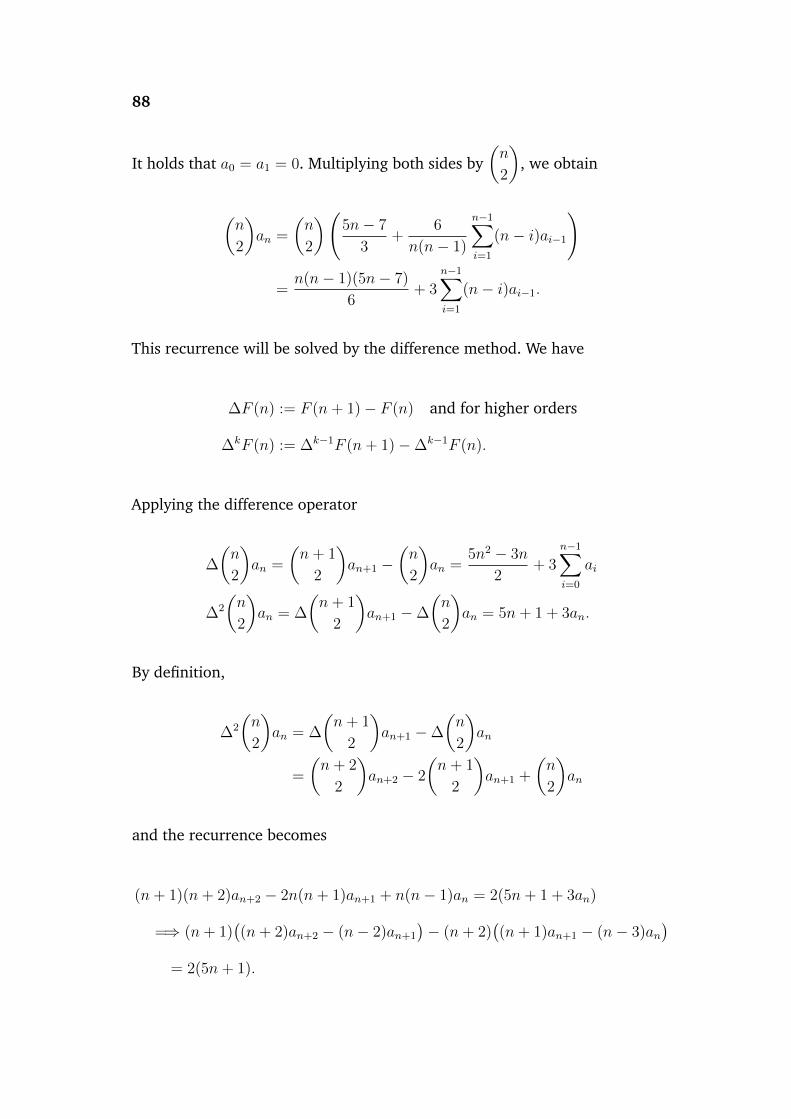
88
It holds that a0 = a1 = 0. Multiplying both sides by(n
2
), we obtain
(n
2
)an =
(n
2
)(5n− 7
3+
6
n(n− 1)
n−1∑i=1
(n− i)ai−1
)
=n(n− 1)(5n− 7)
6+ 3
n−1∑i=1
(n− i)ai−1.
This recurrence will be solved by the difference method. We have
∆F (n) := F (n+ 1)− F (n) and for higher orders
∆kF (n) := ∆k−1F (n+ 1)−∆k−1F (n).
Applying the difference operator
∆
(n
2
)an =
(n+ 1
2
)an+1 −
(n
2
)an =
5n2 − 3n
2+ 3
n−1∑i=0
ai
∆2
(n
2
)an = ∆
(n+ 1
2
)an+1 −∆
(n
2
)an = 5n+ 1 + 3an.
By definition,
∆2
(n
2
)an = ∆
(n+ 1
2
)an+1 −∆
(n
2
)an
=
(n+ 2
2
)an+2 − 2
(n+ 1
2
)an+1 +
(n
2
)an
and the recurrence becomes
(n+ 1)(n+ 2)an+2 − 2n(n+ 1)an+1 + n(n− 1)an = 2(5n+ 1 + 3an)
=⇒ (n+ 1)((n+ 2)an+2 − (n− 2)an+1
)− (n+ 2)
((n+ 1)an+1 − (n− 3)an
)= 2(5n+ 1).
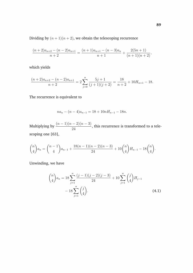
89
Dividing by (n+ 1)(n+ 2), we obtain the telescoping recurrence
(n+ 2)an+2 − (n− 2)an+1
n+ 2=
(n+ 1)an+1 − (n− 3)ann+ 1
+2(5n+ 1)
(n+ 1)(n+ 2),
which yields
(n+ 2)an+2 − (n− 2)an+1
n+ 2= 2
n∑j=0
5j + 1
(j + 1)(j + 2)=
18
n+ 2+ 10Hn+1 − 18.
The recurrence is equivalent to
nan − (n− 4)an−1 = 18 + 10nHn−1 − 18n.
Multiplying by(n− 1)(n− 2)(n− 3)
24, this recurrence is transformed to a tele-
scoping one [63],
(n
4
)an =
(n− 1
4
)an−1 +
18(n− 1)(n− 2)(n− 3)
24+ 10
(n
4
)Hn−1 − 18
(n
4
).
Unwinding, we have
(n
4
)an = 18
n∑j=1
(j − 1)(j − 2)(j − 3)
24+ 10
n∑j=1
(j
4
)Hj−1
− 18n∑j=1
(j
4
). (4.1)
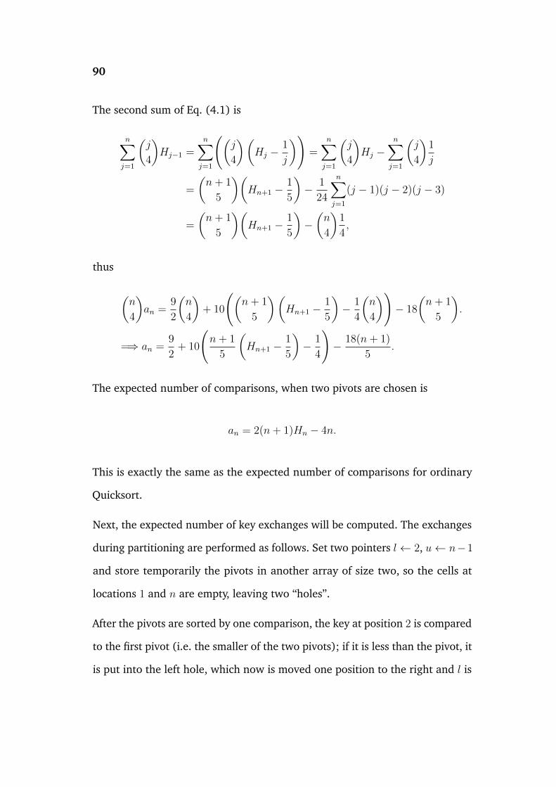
90
The second sum of Eq. (4.1) is
n∑j=1
(j
4
)Hj−1 =
n∑j=1
((j
4
)(Hj −
1
j
))=
n∑j=1
(j
4
)Hj −
n∑j=1
(j
4
)1
j
=
(n+ 1
5
)(Hn+1 −
1
5
)− 1
24
n∑j=1
(j − 1)(j − 2)(j − 3)
=
(n+ 1
5
)(Hn+1 −
1
5
)−(n
4
)1
4,
thus
(n
4
)an =
9
2
(n
4
)+ 10
((n+ 1
5
)(Hn+1 −
1
5
)− 1
4
(n
4
))− 18
(n+ 1
5
).
=⇒ an =9
2+ 10
(n+ 1
5
(Hn+1 −
1
5
)− 1
4
)− 18(n+ 1)
5.
The expected number of comparisons, when two pivots are chosen is
an = 2(n+ 1)Hn − 4n.
This is exactly the same as the expected number of comparisons for ordinary
Quicksort.
Next, the expected number of key exchanges will be computed. The exchanges
during partitioning are performed as follows. Set two pointers l← 2, u← n−1
and store temporarily the pivots in another array of size two, so the cells at
locations 1 and n are empty, leaving two “holes”.
After the pivots are sorted by one comparison, the key at position 2 is compared
to the first pivot (i.e. the smaller of the two pivots); if it is less than the pivot, it
is put into the left hole, which now is moved one position to the right and l is
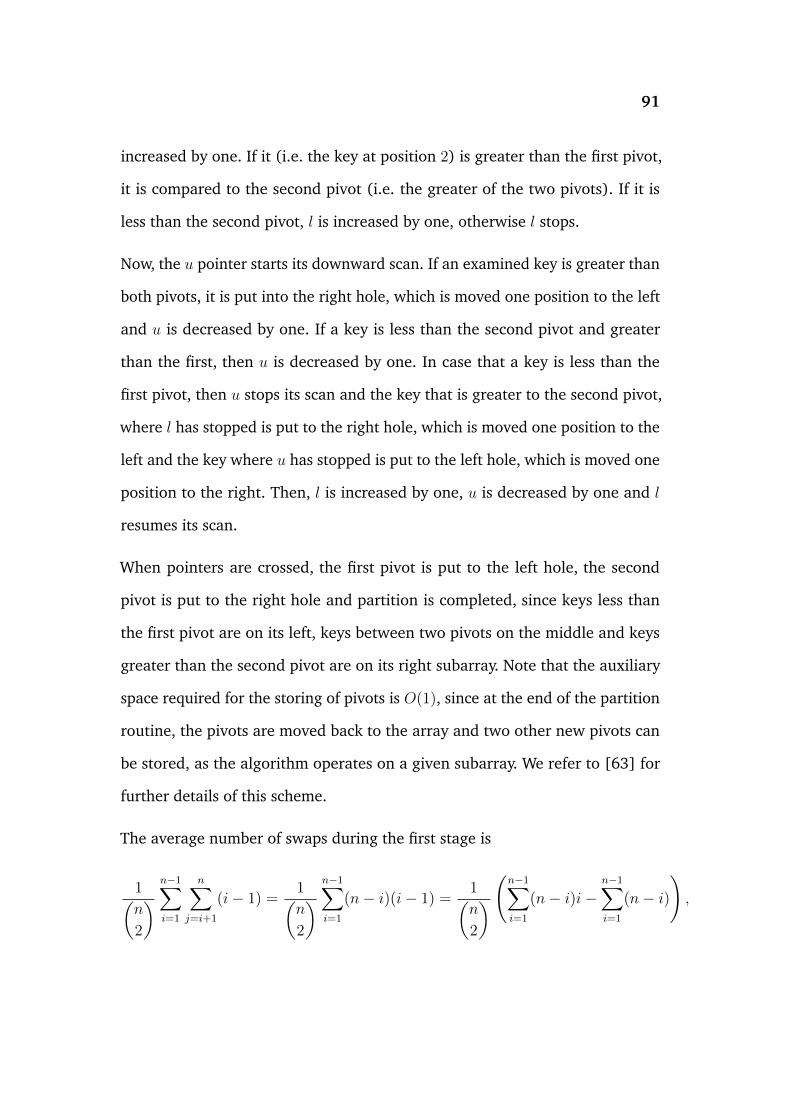
91
increased by one. If it (i.e. the key at position 2) is greater than the first pivot,
it is compared to the second pivot (i.e. the greater of the two pivots). If it is
less than the second pivot, l is increased by one, otherwise l stops.
Now, the u pointer starts its downward scan. If an examined key is greater than
both pivots, it is put into the right hole, which is moved one position to the left
and u is decreased by one. If a key is less than the second pivot and greater
than the first, then u is decreased by one. In case that a key is less than the
first pivot, then u stops its scan and the key that is greater to the second pivot,
where l has stopped is put to the right hole, which is moved one position to the
left and the key where u has stopped is put to the left hole, which is moved one
position to the right. Then, l is increased by one, u is decreased by one and l
resumes its scan.
When pointers are crossed, the first pivot is put to the left hole, the second
pivot is put to the right hole and partition is completed, since keys less than
the first pivot are on its left, keys between two pivots on the middle and keys
greater than the second pivot are on its right subarray. Note that the auxiliary
space required for the storing of pivots is O(1), since at the end of the partition
routine, the pivots are moved back to the array and two other new pivots can
be stored, as the algorithm operates on a given subarray. We refer to [63] for
further details of this scheme.
The average number of swaps during the first stage is
1(n
2
) n−1∑i=1
n∑j=i+1
(i− 1) =1(n
2
) n−1∑i=1
(n− i)(i− 1) =1(n
2
) (n−1∑i=1
(n− i)i−n−1∑i=1
(n− i)
),
92
since (i− 1) keys are less than pivot i. Thus, the average contribution is
2
n(n− 1)
(n3 − n
6− n(n− 1)
2
)=n− 2
3.
For the (n− j) keys greater than j the average value is the same, because the
sums are equal. Adding the two final “exchanges” to get the pivots in place, the
average number of exchanges during the partitioning routine is(
2(n+ 1)
3
).
Letting Sn,2 denote the number of exchanges of dual pivot Quicksort, the recur-
rence for the mean number of exchanges in course of the algorithm is
E(Sn,2) =2(n+ 1)
3+
2
n(n− 1)
×
(n−1∑i=1
n∑j=i+1
E(Si−1,2) +n−1∑i=1
n∑j=i+1
E(Sj−i−1,2) +n−1∑i=1
n∑j=i+1
E(Sn−j,2)
)
=2(n+ 1)
3+
6
n(n− 1)
n−1∑i=1
(n− i)E(Si−1,2).
Multiplying both sides by(n
2
),
(n
2
)E(Sn,2) =
n(n− 1)(n+ 1)
3+ 3
n−1∑i=1
(n− i)E(Si−1,2).
This recurrence is solved in [63]: here we present a solution using generating
functions. Letting bn = E(Sn,2) and g(z) =∑∞
n=0 bnzn be the generating func-
tion of the average number of exchanges, the recurrence is transformed to the
following differential equation:
z2
2
d2g(z)
dz2=z2
3
d3
dz3
(∞∑n=0
zn+1
)+ 3
∞∑n=1
n∑i=1
(n− i)bi−1zn.
93
The double sum is equal to
∞∑n=1
n∑i=1
(n− i)bi−1zn = b0z
2 + (2b0 + b1)z3 + (3b0 + 2b1 + b2)z4 + . . .
= z2(b0 + b1z + b2z2 + . . .) + 2z3(b0 + b1z + b2z
2 + . . .) + . . .
= (z2 + 2z3 + 3z4 + . . .)g(z)
=
( ∞∑n=0
nzn+1
)g(z)
and our differential equation becomes
z2
2
d2g(z)
dz2=
2z2
(1− z)4+ 3g(z)
(z
1− z
)2
.
Changing variables v = 1− z, we have f (k)(v) = (−1)kg(k)(1− v). Thus,
(1− v)2
2
d2f(v)
dv2=
2(1− v)2
v4+ 3f(v)
(1− vv
)2
.
The differential equation can be simplified by multiplying both sides by(
v
1− v
)2
,
v2
2
d2f(v)
dv2=
2
v2+ 3f(v). (4.2)
An elementary approach to solving this differential equation, is to assume that
the solution is of the form xm [9]. Substituting the “trial solution” to Eq. (4.2),
the characteristic or indicial polynomial is
P2(m) = m(m− 1)− 6,
94
with roots m1 = 3 and m2 = −2. Thus, the solution to the corresponding
homogeneous equation is c1v3 + c2v
−2, with c1, c2 ∈ R. A particular solution of
Eq. (4.2), which can be found e.g. using the method in [61], is
−4
5loge(v)v−2.
By the initial conditions f(1) = −f ′(1) = 0, the solution is
f(v) =4
25v3 − 20 loge(v) + 4
25v2.
In the next section, we will examine the generalised version of this differential
equation. Reverting to variable z and discarding terms for n ≤ 3, we see that,
expanding out the fraction term as a series,
g(z) =∞∑n=0
(4
5
((n+ 1)Hn − n
)− 4
25(n+ 1)
)zn.
Finally, the mean number of swaps of dual pivot Quicksort is
bn,2 =4
5(n+ 1)Hn −
24n+ 4
25,
which is nearly 2.4 times greater than the expected number of exchanges of
standard Quicksort.
The recurrence for the number of partitioning stages Pn,2 is much simpler;
Pn,2 = 1 + Pi−1,2 + Pj−i−1,2 + Pn−j,2.
95
By the same reasoning, as in the derivation of the expected number of ex-
changes, the solution is
E(Pn,2) =2
5(n+ 1)− 1
2.
4.1.1 The variance of the number of key comparisons
It is desirable to compute the variance of the number of key comparisons of dual
pivot Quicksort, as this measure provides a grip of the deviation of the random
number of comparisons from its expected value. By the recursive relation, we
have
P(Cn,2 = t) =1(n
2
) n−1∑i=1
n∑j=i+1
P(An,2 + Ci−1,2 + Cj−i−1,2 + Cn−j,2 = t),
noting that the resulting subarrays are independently sorted, the above is
1(n
2
) n−1∑i=1
n∑j=i+1
∑l,m
(P(Ci−1,2 = l)P(Cj−i−1,2 = m)P(Cn−j,2 = t−m− l − 2n+ i+ 2)
).
Letting fn(z) =∞∑t=0
P(Cn,2 = t)zt be the ordinary probability generating func-
tion for the number of comparisons needed to sort n keys, we obtain
fn(z) =1(n
2
) n−1∑i=1
n∑j=i+1
z2n−i−2fi−1(z)fj−i−1(z)fn−j(z). (4.3)
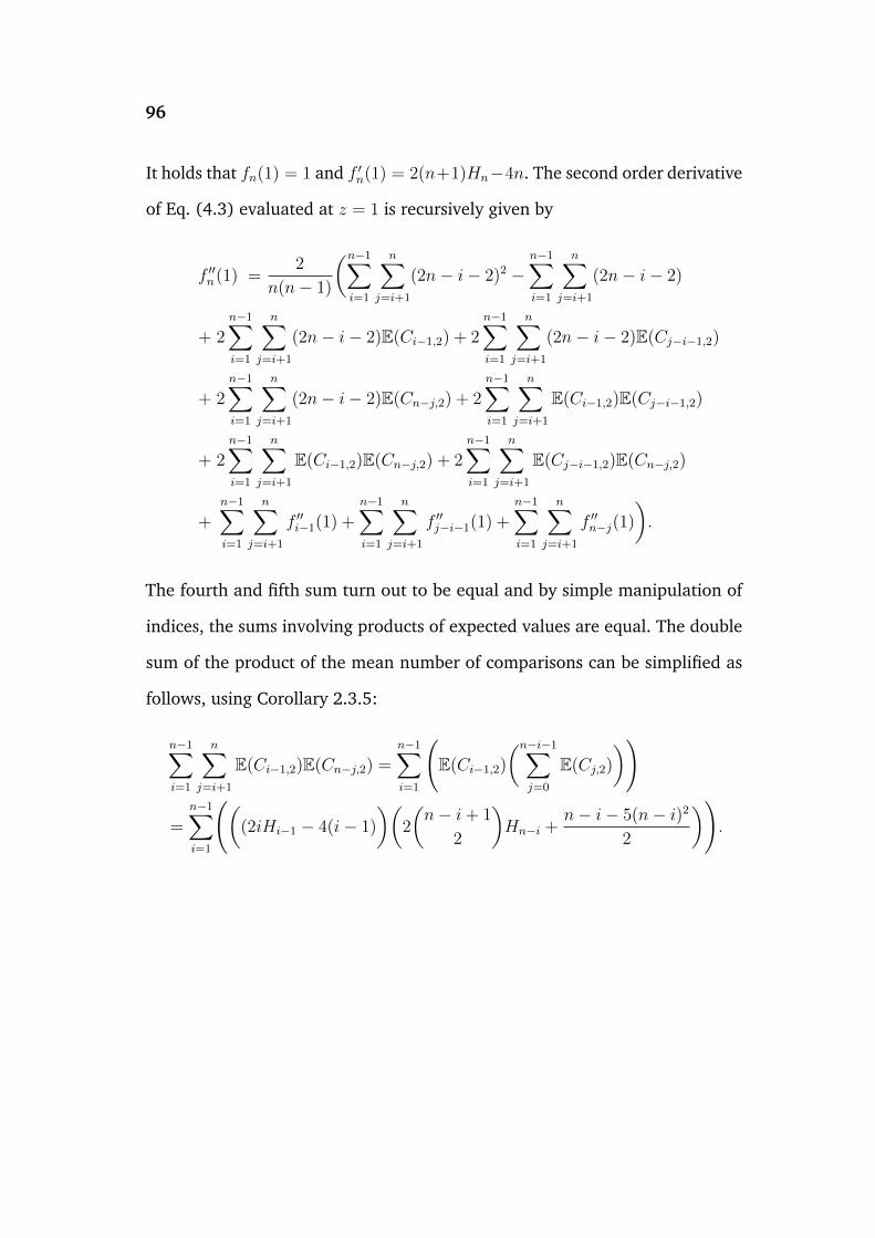
96
It holds that fn(1) = 1 and f ′n(1) = 2(n+1)Hn−4n. The second order derivative
of Eq. (4.3) evaluated at z = 1 is recursively given by
f ′′n(1) =2
n(n− 1)
(n−1∑i=1
n∑j=i+1
(2n− i− 2)2 −n−1∑i=1
n∑j=i+1
(2n− i− 2)
+ 2n−1∑i=1
n∑j=i+1
(2n− i− 2)E(Ci−1,2) + 2n−1∑i=1
n∑j=i+1
(2n− i− 2)E(Cj−i−1,2)
+ 2n−1∑i=1
n∑j=i+1
(2n− i− 2)E(Cn−j,2) + 2n−1∑i=1
n∑j=i+1
E(Ci−1,2)E(Cj−i−1,2)
+ 2n−1∑i=1
n∑j=i+1
E(Ci−1,2)E(Cn−j,2) + 2n−1∑i=1
n∑j=i+1
E(Cj−i−1,2)E(Cn−j,2)
+n−1∑i=1
n∑j=i+1
f ′′i−1(1) +n−1∑i=1
n∑j=i+1
f ′′j−i−1(1) +n−1∑i=1
n∑j=i+1
f ′′n−j(1)
).
The fourth and fifth sum turn out to be equal and by simple manipulation of
indices, the sums involving products of expected values are equal. The double
sum of the product of the mean number of comparisons can be simplified as
follows, using Corollary 2.3.5:
n−1∑i=1
n∑j=i+1
E(Ci−1,2)E(Cn−j,2) =n−1∑i=1
(E(Ci−1,2)
(n−i−1∑j=0
E(Cj,2)
))
=n−1∑i=1
(((2iHi−1 − 4(i− 1)
)(2
(n− i+ 1
2
)Hn−i +
n− i− 5(n− i)2
2
)).
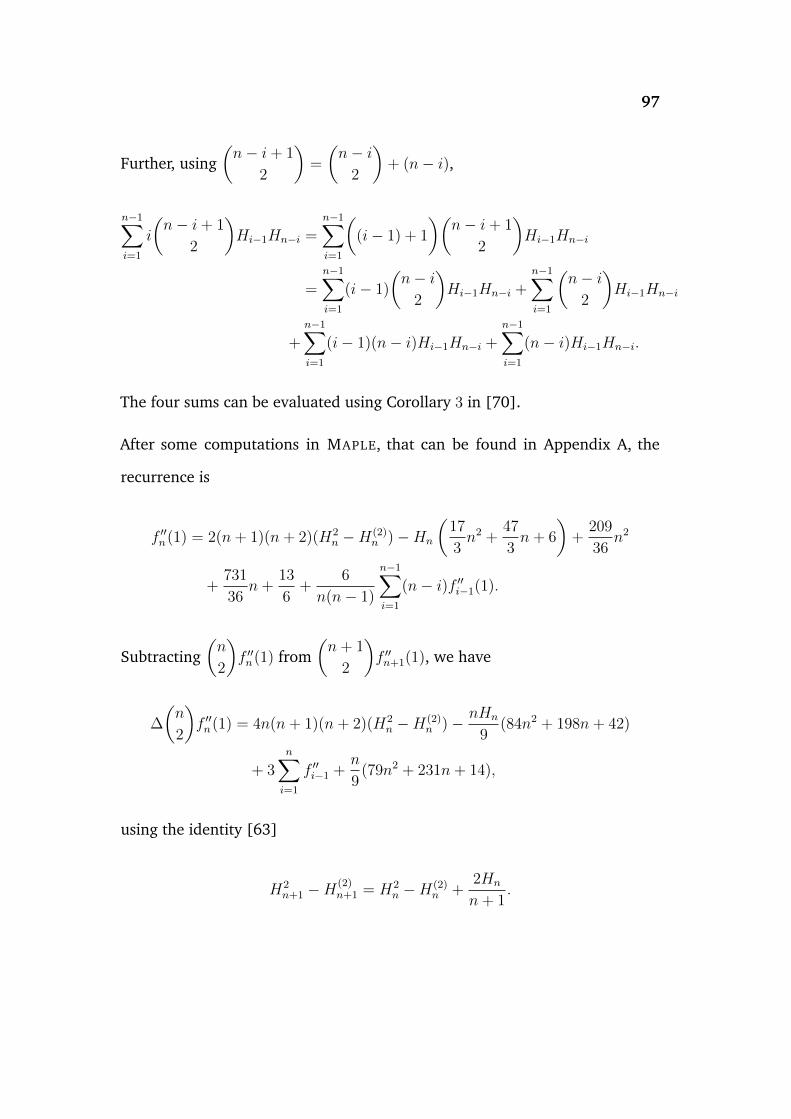
97
Further, using(n− i+ 1
2
)=
(n− i
2
)+ (n− i),
n−1∑i=1
i
(n− i+ 1
2
)Hi−1Hn−i =
n−1∑i=1
((i− 1) + 1
)(n− i+ 1
2
)Hi−1Hn−i
=n−1∑i=1
(i− 1)
(n− i
2
)Hi−1Hn−i +
n−1∑i=1
(n− i
2
)Hi−1Hn−i
+n−1∑i=1
(i− 1)(n− i)Hi−1Hn−i +n−1∑i=1
(n− i)Hi−1Hn−i.
The four sums can be evaluated using Corollary 3 in [70].
After some computations in MAPLE, that can be found in Appendix A, the
recurrence is
f ′′n(1) = 2(n+ 1)(n+ 2)(H2n −H(2)
n )−Hn
(17
3n2 +
47
3n+ 6
)+
209
36n2
+731
36n+
13
6+
6
n(n− 1)
n−1∑i=1
(n− i)f ′′i−1(1).
Subtracting(n
2
)f ′′n(1) from
(n+ 1
2
)f ′′n+1(1), we have
∆
(n
2
)f ′′n(1) = 4n(n+ 1)(n+ 2)(H2
n −H(2)n )− nHn
9(84n2 + 198n+ 42)
+ 3n∑i=1
f ′′i−1 +n
9(79n2 + 231n+ 14),
using the identity [63]
H2n+1 −H
(2)n+1 = H2
n −H(2)n +
2Hn
n+ 1.
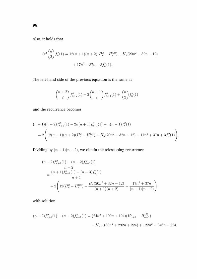
98
Also, it holds that
∆2
(n
2
)f ′′n(1) = 12(n+ 1)(n+ 2)(H2
n −H(2)n )−Hn(20n2 + 32n− 12)
+ 17n2 + 37n+ 3f ′′n(1).
The left-hand side of the previous equation is the same as
(n+ 2
2
)f ′′n+2(1)− 2
(n+ 1
2
)f ′′n+1(1) +
(n
2
)f ′′n(1)
and the recurrence becomes
(n+ 1)(n+ 2)f ′′n+2(1)− 2n(n+ 1)f ′′n+1(1) + n(n− 1)f ′′n(1)
= 2
(12(n+ 1)(n+ 2)(H2
n −H(2)n )−Hn(20n2 + 32n− 12) + 17n2 + 37n+ 3f ′′n(1)
).
Dividing by (n+ 1)(n+ 2), we obtain the telescoping recurrence
(n+ 2)f ′′n+2(1)− (n− 2)f ′′n+1(1)
n+ 2
=(n+ 1)f ′′n+1(1)− (n− 3)f ′′n(1)
n+ 1
+ 2
(12(H2
n −H(2)n )− Hn(20n2 + 32n− 12)
(n+ 1)(n+ 2)+
17n2 + 37n
(n+ 1)(n+ 2)
),
with solution
(n+ 2)f ′′n+2(1)− (n− 2)f ′′n+1(1) = (24n2 + 100n+ 104)(H2n+1 −H
(2)n+1)
−Hn+1(88n2 + 292n+ 224) + 122n2 + 346n+ 224,
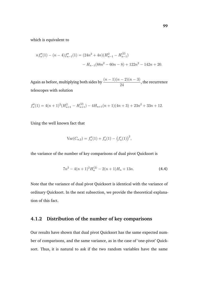
99
which is equivalent to
nf ′′n(1)− (n− 4)f ′′n−1(1) = (24n2 + 4n)(H2n−1 −H
(2)n−1)
−Hn−1(88n2 − 60n− 8) + 122n2 − 142n+ 20.
Again as before, multiplying both sides by(n− 1)(n− 2)(n− 3)
24, the recurrence
telescopes with solution
f ′′n(1) = 4(n+ 1)2(H2n+1 −H
(2)n+1)− 4Hn+1(n+ 1)(4n+ 3) + 23n2 + 33n+ 12.
Using the well known fact that
Var(Cn,2) = f ′′n(1) + f ′n(1)−(f ′n(1)
)2,
the variance of the number of key comparisons of dual pivot Quicksort is
7n2 − 4(n+ 1)2H(2)n − 2(n+ 1)Hn + 13n. (4.4)
Note that the variance of dual pivot Quicksort is identical with the variance of
ordinary Quicksort. In the next subsection, we provide the theoretical explana-
tion of this fact.
4.1.2 Distribution of the number of key comparisons
Our results have shown that dual pivot Quicksort has the same expected num-
ber of comparisons, and the same variance, as in the case of ‘one-pivot’ Quick-
sort. Thus, it is natural to ask if the two random variables have the same
100
distribution. We now show this, after an argument sketched by Prof. Colin
McDiarmid [52].
Suppose that an array of n distinct keys x1, x2, . . . , xn is to be sorted by Quick-
sort and let, as usual, Cn be the random number of comparisons required for
the sorting. Obviously, C1 = 0, C2 = 1 and for n ≥ 3 we pick uniformly at
random an ordered pair of distinct indices (I, J) in [n] = 1, 2, . . . , n and we
use xI as the first pivot. Given that I = i, the pivot xi partitions the array of n
keys to the subarray of (i − 1) keys less than xi and to the subarray of (n − i)
keys greater than xi by (n− 1) comparisons.
Given that I = i, if xJ < xi, then xJ is a uniformly at random chosen pivot from
the subarray of (i− 1) elements less than xi. In this case, for I = i and J = j,
the subarray of (i−1) keys is partitioned to the subarray of (j−1) keys less than
xj and to the subarray of (i− j− 1) keys greater than xj by (i− 2) comparisons.
Note that (i − 2) keys are compared to both pivots in two partitioning stages.
Therefore, the following recurrence holds:
P(Cn = t) =1(n
2
) n−1∑j=1
n∑i=j+1
P((n− 1) + (i− 2) + C
(1)j−1 + C
(2)i−j−1 + C
(3)n−i = t
)
=2
n(n− 1)
n−1∑j=1
n∑i=j+1
P((n+ i− 3) + C
(1)j−1 + C
(2)i−j−1 + C
(3)n−i = t
),
where C(1)n , C(2)
n and C(3)n are independent copies of Cn – that is, are ran-
dom variables with the same distribution as Cn, independent of it and each
other.
If xJ > xi, then xJ is a uniformly at random selected pivot from the subarray
of (n − i) keys greater than xi. Given that I = i and J = j, the subarray of
101
(n − i) keys is partitioned to the subarray of (j − i − 1) keys less than xj and
to the subarray of (n− j) keys greater than xj by (n− i− 1) comparisons. The
recurrence relation is
P(Cn = t) =1(n
2
) n−1∑i=1
n∑j=i+1
P((n− 1) + (n− i− 1) + C
(1)i−1 + C
(2)j−i−1 + C
(3)n−j = t
)
=2
n(n− 1)
n−1∑i=1
n∑j=i+1
P((2n− i− 2) + C
(1)i−1 + C
(2)j−i−1 + C
(3)n−j = t
),
where as in the previous recurrence, C(1)n , C(2)
n and C(3)n are independent copies
of Cn. Observe that
n−1∑j=1
n∑i=j+1
(n+ i− 3) =n−1∑j=1
(n− j)(2n− j − 2) =n−1∑i=1
n∑j=i+1
(2n− i− 2),
thus for any two pivots selected uniformly at random, the recurrences are the
same.
Recall that for the random number of comparisons Cn,2 of dual pivot Quicksort,
it holds that C1,2 = 0, C2,2 = 1 and for n ≥ 3 we choose uniformly at random an
ordered pair of distinct indices (I, J) in [n] = 1, 2, . . . , n. The pivots xI and xJ
are sorted by one comparison and we assume that its outcome is xI < xJ . Given
that I = i and J = j, the array is partitioned to the subarray of (i− 1) keys less
than xi, the subarray of (j − i− 1) keys between two pivots and the subarray
of (n− j) keys greater than xj. Since keys greater than xi are compared with
the other pivot as well, the recurrence for the random number of comparisons
102
is
P(Cn,2 = t) =1(n
2
) n−1∑i=1
n∑j=i+1
P(1 + (i− 1) + 2(j − i− 1) + 2(n− j)
+ C(1)i−1,2 + C
(2)j−i−1,2 + C
(3)n−j,2 = t
)=
2
n(n− 1)
n−1∑i=1
n∑j=i+1
P((2n− i− 2) + C
(1)i−1,2 + C
(2)j−i−1,2 + C
(3)n−j,2 = t
),
where C(1)n,2, C(2)
n,2 and C(3)n,2 are independent copies of Cn,2. Note that when xI >
xJ , the recurrence is the same. Thus, since dual pivot Quicksort and ordinary
Quicksort satisfy the same recurrence and have the same initial conditions for
n = 1, 2, we deduce that the random variables Cn,2 and Cn are identically
distributed.
4.2 Multikey partitioning
A natural extension of having two pivots would be to have some other number
k of pivots. Here, we study the idea of randomly picking k pivots i1, i2, . . . , ik
and partitioning the array simultaneously according to these.
Again, let a random permutation of the array 1, 2, . . . , n be given to be sorted
using this variant, with all the n! permutations equally likely to be the input.
The k rightmost keys are chosen as pivots, are compared to each other and
exchanged, if they are out of order. The sorting of the pivots can be efficiently
implemented by insertion sort. Since all n! permutations of the keys are equally
likely to be the input, this amounts to the fact that any k-subset of keys has
equal probability to be selected.

103
The remaining (n− k) keys are compared to the pivots and the array is parti-
tioned to (k + 1) subarrays. The partitioning can be performed as follows. We
compare the leftmost key to a randomly chosen pivot; if it is smaller than this
pivot, it is compared with another smaller pivot (if one exists). Otherwise it is
compared with a larger pivot (to the right) and after a series of comparisons, is
inserted to its place between any two pivots, or to the left of the smallest pivot
or to the right of the greatest pivot. We continue in the same fashion, until all
keys are examined.
In [28], each of the (n − k) keys is compared to the pivots by binary search,
so a key is compared first to the median of the sorted array of the pivots. If
it is less, is compared with the first quartile, otherwise is compared with the
third quartile and after a series of comparisons is inserted to its position. In
worst case, it takes O(log2(k)
)comparisons for the insertion of a key. Then,
multipivot Quicksort is recursively applied to each of the resulting segments
that contains at least (k + 1) keys and arrays with less than (k + 1) keys are
sorted by insertion sort in O(n) time.
This is equivalent to (k+ 1)-ary search trees, which is a generalisation of binary
trees. Indeed, if n ≥ k + 1, the k pivots are stored in the root node of the tree
in increasing order and the remaining (n− k) keys are placed in the resulting
(k + 1) subtrees of the root. In case that n = 0, the tree is empty and if n ≤ k,
the tree has a single node, which stores the keys in order. Under the assumption
of uniformity, this is a (k+ 1)-random tree of n nodes – see the article of Chern
et al. [14] and Mahmoud’s book [49] for the correspondence between trees
and variants of Quicksort.
104
Let f(n, k) denote the expected cost of the algorithm applied to an array of
n keys. We deliberately allow some flexibility in the form of cost; a typical
example might be the number of comparisons. The expected cost of this variant
is recursively given by
f(n, k) = T (n, k)
+1(n
k
)∑i′1
∑i′2
. . .∑i′k︸ ︷︷ ︸
i′1<i′2<...<i
′k
(f(i′1 − 1, k) + f(i′2 − i′1 − 1, k) + . . .+ f(n− i′k, k)
),
where i′1 < i′2 < . . . < i′k are the pivots in increasing order, T (n, k) = a(k)n+b(k)
is the average value of a “toll function” τ(n, k) during the first recursive call
and f(i′1 − 1, k) denotes the average cost for sorting the subarray of (i′1 − 1)
elements less than i′1 by multipivot Quicksort on k pivots.
Though this looks a complex k-index summation, the recursion can be sim-
plified, by noting that the pivots are randomly selected and the sums are
equal,
f(n, k) = T (n, k)
+1(n
k
)∑i′1
∑i′2
. . .∑i′k︸ ︷︷ ︸
i′1<i′2<...<i
′k
(f(i′1 − 1, k) + f(i′2 − i′1 − 1, k) + . . .+ f(n− i′k, k)
)
= T (n, k) +1(n
k
) n−k+1∑i′1=1
n−k+2∑i′2=i′1+1
. . .
n∑i′k=i′k−1+1
(f(i′1 − 1, k) + . . .+ f(n− i′k, k)
)
= T (n, k) +(k + 1)!
n(n− 1) . . . (n− k + 1)
n−k+1∑i′1=1
(n− i1k − 1
)f(i′1 − 1, k).
105
Multiplying both sides by(n
k
), the recurrence relation becomes
(n
k
)f(n, k) =
(n
k
)T (n, k) + (k + 1)
n−k+1∑i′1=1
(n− i′1k − 1
)f(i′1 − 1, k).
For notational convenience, let f(n, k) = an and consider the generating func-
tion h(x) =∞∑n=0
anxn;
∞∑n=0
(n
k
)anx
n =∞∑n=0
(n
k
)T (n, k)xn + (k + 1)
∞∑n=0
n∑i′1=1
(n− i′1k − 1
)ai′1−1
xn.
The recurrence is transformed to a k-th order differential equation
h(k)(x)xk
k!=∞∑n=0
(n
k
)T (n, k)xn + h(x)(k + 1)
∞∑n=0
(n− 1
k − 1
)xn
=∞∑n=0
(n
k
)(a(k)n+ b(k)
)xn + (k + 1)h(x)
(x
1− x
)k=xk(a(k)(x+ k) + b(k)(1− x)
)(1− x)k+2
+ (k + 1)h(x)
(x
1− x
)k,
since it can be easily seen by induction that the k-th order derivative of
∞∑n=0
(a(k)n+ b(k)
)xn =
a(k)x+ b(k)(1− x)
(1− x)2
isk!(a(k)(x+ k) + b(k)(1− x)
)(1− x)k+2
.
106
Multiplying by(
x
1− x
)−k, the differential equation is simplified to
h(k)(x)(1− x)k
k!=a(k)(x+ k) + b(k)(1− x)
(1− x)2+ (k + 1)h(x).
This differential equation is an equidimensional Cauchy–Euler equation, as the
one encountered in the previous Chapter. Changing variables x = 1 − z, it is
h(x) = g(1 − x). Applying the differential operator Θ, where Θg(z) = zg′(z),
the differential equation becomes
((−1)kΘ(Θ− 1) . . . (Θ− k + 1)− (k + 1)!
)g(z) =
k!(a(k)(1− z + k) + b(k)z
)z2
and the indicial polynomial Pk(Θ) is equal to
Pk(Θ) = (−1)kΘk − (k + 1)!.
Using the notation from [26], Θk = Θ(Θ−1) . . . (Θ−k+1) with k ≥ 0, denotes
the falling factorial. Again, we need a Lemma regarding the roots of the indicial
polynomial.
Lemma 4.2.1. The indicial polynomial Pk(Θ) has k simple roots with real parts
in the interval [−2, k + 1]. The real roots are −2; (k + 1), if k is even and the
2⌊k−1
2
⌋complex roots α1, . . . , αb k−1
2 c with their conjugates α1, . . . , αb k−12 c.

107
Proof. Let α = x+ iy be a root of the polynomial. It holds
α(α− 1) . . . (α− k + 1) = (−1)k(k + 1)!
=⇒ α(α− 1) . . . (α− k + 1) = (−2)(−3) . . .(−(k + 1)
)=⇒ α
−2
α− 1
−3. . .
α− k + 1
−(k + 1)= 1. (4.5)
Suppose that Re(α) < −2. Then
∣∣∣∣ α−2
∣∣∣∣ =
√x2 + y2
2>
√(−2)2 + y2
2≥ 1∣∣∣∣α− 1
−3
∣∣∣∣ =
√(x− 1)2 + y2
3>
√(−3)2 + y2
3≥ 1
...∣∣∣∣α− (k − 1)
−(k + 1)
∣∣∣∣ =
√(x− (k − 1)
)2+ y2
k + 1>
√(−(k + 1)
)2+ y2
k + 1≥ 1.
Considering the moduli in Eq. (4.5), we see that the left-hand side is a product
of numbers which are all greater than 1, and so the overall product is greater
than 1, but the right-hand side is equal to 1, leading to contradiction. Therefore
every root has real part greater than or equal to −2. Further, looking over the
same argument, we see that the only way we can have the real part being equal
to −2 is if the imaginary part is equal to zero.
108
By the Fundamental Theorem of Algebra a polynomial of degree n has n com-
plex roots with multiplicities. Note that −2 is always a simple root since,
Pk(−2) = (−1)k(−2)(−3) . . .(−(k + 1)
)− (k + 1)!
= (−1)2k(k + 1)!− (k + 1)! = 0,
P ′k(−2) = (k + 1)!k−1∑j=0
1
−2− j= −(k + 1)!(Hk+1 − 1) < 0.
Suppose that α is a repeated root. Since Re(α) ≥ −2, we can write α =
(x− 2) + iy with x ≥ 0. By the above comments we have that
k−1∑j=0
1
α− j= 0
=⇒k−1∑j=0
1
(x− 2− j) + iy= 0
=⇒k−1∑j=0
(x− 2− j)− iy(x− 2− j)2 + y2
= 0
In particular, Im(α) = 0. But that imaginary part is equal to∑k−1
j=0y
(x−2−j)2+y2
which is clearly only equal to zero if y = 0 i.e. the root is real. We will thus
have obtained our contradiction if we can show that there are no real roots
other than −2 and (for k even) k + 1.
To do this, suppose that we did have a real root α > −2. We note first that
α > 0: because if not, then since −2 is also a root, there is a root of P ′ between
−2 and 0 by Rolle’s Theorem. But since P ′k(β) = 0 implies that∑k−1
j=01
β−j =
0 and when β < 0 this number is clearly negative. Thus any real root α is
positive. It is also ≤ k + 1 as if it were greater than k + 1 we would have

109
α(α − 1) . . . (α − k + 1) > (k + 1)!. Further, note that k + 1 is a root if and
only if k is even and there cannot be a root in α ∈ [k, k + 1) as the product
α(α− 1) . . . (α− k + 1) would be < (k + 1)!.
Suppose then that α ∈ (j, j + 1) for some 0 ≤ j ≤ k − 1. Then the product of
the non-negative numbers in the sequence α, α − 1, . . . , α − k + 1 is at most
α(α− 1) . . . (α− j) ≤ (j + 1) . . . 2 · 1 = (j + 1)!. Thus, to get α being a root, we
have to have that
(−1)k(α− j − 1) . . . (α− k + 1) ≥ (k + 1)!
(j + 1)!= (j + 2)(j + 3) . . . (k + 1).
However the largest in modulus of α−j−1, . . . , α−k+1 is α−k+1 > j+1−k
and so their product is less than (k − 1 − j)!. Consequently our inequalities
together imply
(k + 1)!
(j + 1)!(k − 1− j)!< 1 =⇒ (k + 1)
(k
j + 1
)< 1
and this is a contradiction, completing the proof.
The differential equation can be written as
Sk−1(Θ)(Θ + 2)g(z) =k!(a(k)(1− z + k) + b(k)z
)z2
.
Letting rk = −2 and the remaining (k − 1) simple roots be r1, r2, . . . , rk−1, we
have
(Θ− r1) . . . (Θ− rk−1)(Θ + 2)g(z) =k!(a(k)(1− z + k) + b(k)z
)z2
.
110
For the solution of our differential equation, let two functions g1(z) + g2(z) =
g(z). Then
(Θ− r1) . . . (Θ− rk−1)(Θ + 2)(g1(z) + g2(z)
)=a(k)(k + 1)!
z2+
(b(k)− a(k))k!
z
and by the property of linearity of differential operator
(Θ− r1) . . . (Θ− rk−1)(Θ + 2)g1(z) =a(k)(k + 1)!
z2
(Θ− r1) . . . (Θ− rk−1)(Θ + 2)g2(z) =
(b(k)− a(k)
)k!
z.
In the same manner as in the analysis of ‘median of (2k+1)’ Quicksort, applying
k times the solution, we obtain
g1(z) =a(k)(k + 1)!
(−2− r1)(−2− r2) . . . (−2− rk−1)
loge(z)
z2+
k∑i=1
cizri
g2(z) =k!
(−1− r1)(−1− r2) . . . 1
(b(k)− a(k))
z+
k∑i=1
dizri ,
where ci and di are constants of integration. In order to evaluate Sk−1(−2),
note that
Sk−1(−2) = P ′k(−2),
thus
Sk−1(−2) = −(k + 1)!(Hk+1 − 1).
Moreover,
Pk(−1) = −kk!.
111
Combining both solutions,
g(z) = − a(k)
Hk+1 − 1
loge(z)
z2+
1
k
(a(k)− b(k))
z+
k∑i=1
sizri , (4.6)
where si = ci + di. The constants of integration can be found solving the
following system of equations
g(1) = g′(1) = . . . = g(k−1)(1) = 0.
In terms of series;
h(x) =a(k)
Hk+1 − 1
∞∑n=0
((n+ 1)Hn − n)
)xn +
∞∑n=0
k∑i=1
si(−1)n(rin
)xn
+a(k)− b(k)
k
∞∑n=0
xn. (4.7)
The third sum of Eq. (4.7) adds to the solution a constant negligible contribu-
tion. Also, the root (k + 1), when k is even, contributes a constant and the root
rk = −2, adds sk(n+ 1), with sk ∈ R. Extracting the coefficients, the expected
cost of multipivot Quicksort is
an =a(k)
Hk+1 − 1
((n+ 1)Hn − n
)+ sk(n+ 1) + 2
b k−12c∑
i=1
(−1)nRe
(si
(αin
))+O(1).
The asymptotics of the last sum can be found by the well-known Stirling’s
formula, that states [26]
n! ∼√
2πn(ne
)n.
112
Expressing the binomial coefficient in terms of Γ functions, we have
(−1)n(αin
)=
(−αi + n− 1
n
)=
Γ(n− αi)n!Γ(−αi)
.
The relation 6.1.26 in [1] reads for x, y ∈ R,
|Γ(x+ iy)| ≤ |Γ(x)|,
thus
|Γ(n− αi)| ≤ |Γ(n−Re(αi)
)|.
Using Stirling’s formula,
Γ(n−Re(αi))
n!∼
√2π
(n−
(Re(αi) + 1
))(n− (Re(αi) + 1)
e
)n−(Re(αi)+1
)√
2πn
(n
e
)n
∼
(n−
(Re(αi) + 1
)e
)n−(Re(αi)+1
)(n
e
)n
=
(n−
(Re(αi) + 1
)e
)−(Re(αi)+1) (
1− Re(αi) + 1
n
)n∼ Cn−(Re(αi)+1),
where C = e−(Re(αi)+1) is an unimportant constant.
Therefore the term is bounded by
2(−1)nRe
(si
(αin
))= O(n−(Re(αi)+1))
113
and asymptotically, the expected cost is
a(k)
Hk+1 − 1n loge(n) +
(sk +
a(k)
Hk+1 − 1(γ − 1)
)n+ o(n),
since all the other roots have real parts greater than −2.
Knowing the coefficients, any mean cost of the generalisation of the algorithm
can be directly computed, using this solution, which assumes a simple form.
These coefficients are related to the number of pivots used during the partition-
ing scheme. In [28], the average number of comparisons of the first stage is
given by:
a(s)n+O(1),
where s denotes the number of partitions, when s− 1 pivots are used or equiv-
alently the maximum number of descendants of a node of an s–ary tree. The
coefficient a(s)n is equal to
a(s) = dlog2(s)e+s− 2dlog2(s)e
s.
Thus, the average number of comparisons of Quicksort on k pivots is
(dlog2(k + 1)e+ 1− 2dlog2(k+1)e
k+1
Hk+1 − 1
)(n+ 1)Hn +O(n).
114
4.2.1 Derivation of integration constants using Vandermonde
matrices
The constants of integration can be found using Vandermonde matrices. Differ-
entiating m times Eq. (4.6),
g(m)(z) =a(k)
Hk+1 − 1
(−1)m+1m!((m+ 1) loge(z)− ((m+ 1)Hm −m)
)zm+2
+ (−1)mm!
(a(k)− b(k)
)kzm+1
+k∑i=1
sirmi z
ri−m
=(−1)mm!
zm+1
(−a(k)
((m+ 1) loge(z)− ((m+ 1)Hm −m)
)z(Hk+1 − 1)
+
(a(k)− b(k)
)k
)+
k∑i=1
sirmi z
ri−m.
The result can be easily proven by induction or by Leibniz’s product rule. Using
the initial conditions, namely that g and its first (k − 1) derivatives are 0 when
evaluated at z = 1, we obtain
k∑i=1
sirmi = (−1)m+1m!
(a(k)
((m+ 1)Hm −m)
)Hk+1 − 1
+a(k)− b(k)
k
),
for m = 0, 1, . . . , (k − 1). In matrix form, the linear system is
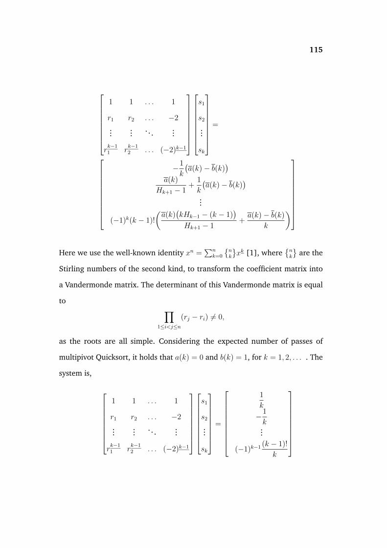
115
1 1 . . . 1
r1 r2 . . . −2
...... . . . ...
rk−11 r
k−12 . . . (−2)k−1
s1
s2
...
sk
=
−1
k
(a(k)− b(k)
)a(k)
Hk+1 − 1+
1
k
(a(k)− b(k)
)...
(−1)k(k − 1)!
(a(k)
(kHk−1 − (k − 1)
)Hk+1 − 1
+a(k)− b(k)
k
)
Here we use the well-known identity xn =∑n
k=0
nk
xk [1], where
nk
are the
Stirling numbers of the second kind, to transform the coefficient matrix into
a Vandermonde matrix. The determinant of this Vandermonde matrix is equal
to ∏1≤i<j≤n
(rj − ri) 6= 0,
as the roots are all simple. Considering the expected number of passes of
multipivot Quicksort, it holds that a(k) = 0 and b(k) = 1, for k = 1, 2, . . . . The
system is,
1 1 . . . 1
r1 r2 . . . −2
...... . . . ...
rk−11 r
k−12 . . . (−2)k−1
s1
s2
...
sk
=
1
k
−1
k...
(−1)k−1 (k − 1)!
k
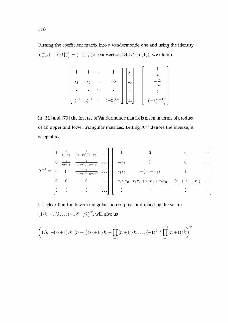
116
Turning the coefficient matrix into a Vandermonde one and using the identity∑nj=0(−1)jj!
nj
= (−1)n, (see subsection 24.1.4 in [1]), we obtain
1 1 . . . 1
r1 r2 . . . −2
...... . . . ...
rk−11 rk−1
2 . . . (−2)k−1
s1
s2
...
sk
=
1
k
−1
k...
(−1)k−1 1
k
In [31] and [73] the inverse of Vandermonde matrix is given in terms of product
of an upper and lower triangular matrices. Letting A−1 denote the inverse, it
is equal to
A−1 =
1 1r1−r2
1(r1−r2)(r1−r3)
. . .
0 1r2−r1
1(r2−r1)(r2−r3)
. . .
0 0 1(r3−r1)(r3−r2)
. . .
0 0 0 . . .
......
... . . .
1 0 0 . . .
−r1 1 0 . . .
r1r2 −(r1 + r2) 1 . . .
−r1r2r3 r1r2 + r1r3 + r2r3 −(r1 + r2 + r3) . . .
......
... . . .
It is clear that the lower triangular matrix, post–multiplied by the vector(1/k,−1/k, . . . (−1)k−1/k
)T, will give us
(1/k,−(r1+1)/k, (r1+1)(r2+1)/k,−
3∏i=1
(ri+1)/k, . . . , (−1)k−1
k−1∏i=1
(ri+1)/k
)T
.
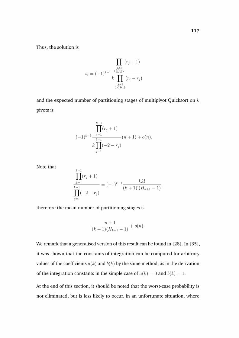
117
Thus, the solution is
si = (−1)k−1
∏j 6=i
1≤j≤k
(rj + 1)
k∏j 6=i
1≤j≤k
(ri − rj)
and the expected number of partitioning stages of multipivot Quicksort on k
pivots is
(−1)k−1
k−1∏j=1
(rj + 1)
kk−1∏j=1
(−2− rj)(n+ 1) + o(n).
Note thatk−1∏j=1
(rj + 1)
k−1∏j=1
(−2− rj)= (−1)k−1 kk!
(k + 1)!(Hk+1 − 1),
therefore the mean number of partitioning stages is
n+ 1
(k + 1)(Hk+1 − 1)+ o(n).
We remark that a generalised version of this result can be found in [28]. In [35],
it was shown that the constants of integration can be computed for arbitrary
values of the coefficients a(k) and b(k) by the same method, as in the derivation
of the integration constants in the simple case of a(k) = 0 and b(k) = 1.
At the end of this section, it should be noted that the worst-case probability is
not eliminated, but is less likely to occur. In an unfortunate situation, where
118
the k smallest or greatest keys are selected as pivots, partitioning will yield
trivial subarrays and one containing the remaining elements. If the chosen
pivots happen to be close to the quantiles of the array, this yields an optimal
partitioning of the array. In the next section, we examine ways of a more
efficient selection of pivots.
4.3 Multipivot–median partitioning
The preceding analysis of multipivot Quicksort, where k pivots are uniformly
selected at random has showed that the worst-case scenario is less likely from
the standard ‘one–pivot’ model. Is any other way, where we can reduce further
the probability of such scenario? We have seen that choosing the median from
a random sample of the array to be sorted, yields savings to the running time
of the algorithm. Since we have examined the analysis of multiple pivots, then
we can select these pivots as the quantiles of a bigger random sample.
Thus, one can randomly choose a larger sample of k(t + 1) − 1 keys, find
the (t + 1)-st, 2(t + 1)-th, . . . , (k − 1)(t + 1)-th smallest keys and use these
(k− 1) statistics as pivots. Note that for k = 2, this variant contains the median
of 2t + 1 Quicksort as a special case and for t = 0, we have the multipivot
algorithm, whose mathematical analysis was presented in the previous section.
This ‘generalised Quicksort’ was introduced by Hennequin [28]. Let T (nk,t)
be the average of a “toll function” during the first pass and f(nk,t) the total
expected cost of this variant, when applied to an array of n keys. The following
119
recurrence (which is not presented so simply in Hennequin) holds:
f(nk,t) = T (nk,t) +1(n
k(t+ 1)− 1
)×∑i1
∑i2
. . .∑ik−1︸ ︷︷ ︸
i1<i2<...<ik−1
((i1 − 1
t
)(i2 − i1 − 1
t
). . .
(ik−1 − ik−2 − 1
t
)(n− ik−1
t
)
·(f((i1 − 1)k,t) + f((i2 − i1 − 1)k,t) + . . .+ f((ik−1 − ik−2 − 1)k,t)
+ f((n− ik−1)k,t))),
since the pivots i1, . . . , ik−1 are selected to be the (t+ 1)-st, . . . , (k− 1)(t+ 1)-th
smallest keys of the sample and each of the k resulting subarrays (i1 − 1), (i2 −
i1 − 1), . . . , (n− ik−1) contain t elements of the sample.
As before, the general recurrence of average cost is translated to a differential
equation with indicial polynomial [28],
Pk(t+1)−1(Θ) = (−1)k(t+1)−1
(Θ
k(t+ 1)− 1
)− k(−1)t
(Θ
t
).
A Lemma follows concerning the whereabouts of the roots of this polyno-
mial:
Lemma 4.3.1. The indicial polynomial Pk(t+1)−1(Θ) has k(t + 1) − 1 simple
roots, with real parts greater than or equal to −2. The real roots are the integers
0, 1, . . . , (t − 1), −2; k(t + 1) + t, when t is odd and k is even or when t is even
and k is odd and the 2⌊
(k−1)t+k−22
⌋complex roots λ1, . . . , λb (k−1)t+k−2
2 c with their
conjugates λ1, . . . , λb (k−1)t+k−22 c.

120
Proof. It can be easily deduced that the integers 0, 1, . . . , (t − 1) and −2 are
roots of the polynomial. Now, when t is odd and k is even, then k(t+ 1)− 1 is
odd and so a root α of the polynomial will satisfy
(α
k(t+ 1)− 1
)= k
(α
t
)(4.8)
and by simple manipulations we can now verify that k(t+ 1) + t is also a root.
Similarly, if t is even and k is odd, we have that k(t + 1) − 1 is even and Eq.
(4.8) is valid, again making k(t+ 1) + t a root.
It will be proved by contradiction that all roots have real parts greater than or
equal to −2. Note that the argument is similar with the proofs of Lemmas 3.1.1
and 4.2.1. For any root r = x+ iy, with x, y ∈ R holds
(−1)k(t+1)−1
(r
k(t+ 1)− 1
)= k(−1)t
(r
t
). (4.9)
For r 6= 0, 1, . . . , (t− 1), Eq. (4.9) can be written as
(−1)k(t+1)−1 (r − t)(r − t− 1) . . .(r − k(t+ 1) + 2
)(t+ 1) . . .
(k(t+ 1)− 1
) = (−1)tk. (4.10)
121
Assume that Re(r) < −2, then
∣∣∣∣r − tt+ 1
∣∣∣∣ =
√(x− t)2 + y2
t+ 1>
√(−(t+ 2)
)2+ y2
t+ 1≥ t+ 2
t+ 1∣∣∣∣r − t− 1
t+ 2
∣∣∣∣ =
√(x− t− 1)2 + y2
t+ 2>
√(−(t+ 3)
)2+ y2
t+ 2≥ t+ 3
t+ 2
...∣∣∣∣∣r −(k(t+ 1)− 2
)k(t+ 1)− 1
∣∣∣∣∣ =
√(x− k(t+ 1) + 2
)2+ y2
k(t+ 1)− 1>
√(−k(t+ 1)
)2+ y2
k(t+ 1)− 1
≥ k(t+ 1)
k(t+ 1)− 1.
Considering the product of moduli, we see that the left-hand side of Eq. (4.10) is
greater than or equal to (in modulus) the telescoping product k(t+1)/(t+1) =
k, which gives a contradiction. Further, this argument shows that −2 is the
unique root with the least real part.
We now show the roots are simple. Assuming, for a contradiction, that r is a
repeated root, we get:
(−1)k(t+1)−1
(r
k(t+ 1)− 1
) k(t+1)−2∑j=0
1
r − j= k(−1)t
(r
t
) t−1∑j=0
1
r − j. (4.11)
Eq. (4.9) and (4.11) imply that
k(t+1)−2∑j=0
1
r − j=
t−1∑j=0
1
r − j
ork(t+1)−2∑
j=t
1
r − j= 0. (4.12)
122
From Eq. (4.12), we deduce that Im(r) = 0 and r ∈ (t, t+ 1) ∪ (t+ 1, t+ 2) ∪
. . . ∪(k(t+ 1)− 3, k(t+ 1)− 2
). However, the modulus in the left-hand side of
Eq. (4.9) is smaller than 1, while the right-hand side is greater than k, proving
that all roots are simple.
By the Lemma, the polynomial can be written in terms of simple factors and
the differential equation can be solved using the same way, as in other variants
of Quicksort, previously analysed. The average cost of ‘generalised Quicksort’
is
a(k, t)
Hk(t+1) −Ht+1
((n+ 1)Hn − n
)+O(n),
when the “toll function” is linear and its average is a(k, t)n+O(1).
Our analyses of the average cost of the algorithm and its variants have showed
that any Quicksort needs on average Cn loge(n) + O(n) key comparisons for
the complete sorting of a file consisting of n distinct keys. The constant C can
be made very close to the information–theoretic bound, as we saw. In many
sorting applications the ‘median of 3’ is being used, with savings on the average
time and little overhead for the computation of median. For large arrays, one
can use the ‘remedian of 32’ Quicksort.
Chapter 5
Partial order of keys
5.1 Introduction
Here, we investigate the analysis of Quicksort under the assumption of prior
information of the order of keys. Specifically, we assume that there is a partial
order on the keys. The rough idea is to see how much having partial information
compatible with the true order allows us to speed up the process of finding the
true order.
Let us illustrate the idea first with a simple example. Suppose that there are
d levels with k keys at each level, so that n = kd. Anything in a higher level
is known to be above everything in a lower level. Computing the ratio of the
expected complexities, we have
E(Cn)
E(C∗n)=d(2(k + 1)Hk − 4k
)2(n+ 1)Hn − 4n
,
where C∗n and Cn denote the number of comparisons of Quicksort with uni-
form pivot selection and in case of partial order, respectively. We consider the
following cases:
123
124
1. When d is fixed number, then as n tends to infinity,
limn→∞
n
d=∞.
Thus,
limn→∞
E(Cn)
E(C∗n)∼ lim
n→∞
d(2k loge(k)
)2n loge(n)
= limn→∞
loge(k)
loge(n)= lim
n→∞
loge(n/d)
loge(n)= 1.
2. d = k =√n.
limn→∞
E(Cn)
E(C∗n)= lim
n→∞
√n(2(√n+ 1)H√n − 4
√n)
2(n+ 1)Hn − 4n∼ lim
n→∞
2n loge(√n)
2n loge(n)=
1
2.
We see that Quicksort is on average twice as fast, when sorting a partially
ordered array.
3. k = 1c
where c is a constant. Then,
limn→∞
E(Cn)
E(C∗n)=cn(2(1
c+ 1)H1/c − 4
c
)2(n+ 1)Hn − 4n
=n((2 + 2c)H1/c − 4
)2n loge(n)
=c′
loge(n),
where c′ =(2 + 2c)H1/c − 4
2.
We should think a little about variability too. It is unsurprising that having
the additional information about levels reduces variability of the number of
comparisons, let us get a preliminary result. If we have the level structure, then
Var(C∗n) is the sum of the variances of sorting each of the d independent levels.
Each of these variances, since there are k keys in each level, is just Var(Ck). For
simplicity, we assume k →∞ as n→∞ and do asymptotics. We then have (for
125
m either n or k)
Var(Cm) ∼(
7− 2π2
3
)·m2
and thus we get
Var(Cn)
Var(C∗n)' (7− 2π2/3)n2
(7− 2π2/3)k2d= d
so the variance of the version with the presorting is reduced by a factor of
about d. These suggest there is interest in studying this situation, we now do
so in more detail.
5.2 Partially ordered sets
An approach of having additional information is the partial order of the keys.
We shall employ this assumption along the following lines. First, we present a
definition [56].
Definition 5.2.1. Let a finite set P equipped with a binary relation ‘≤’ which has
the following properties. (Here, x, y and z are elements of P ).
(i) x ≤ x, ∀x ∈ P . (That is, ≤ is reflexive)
(ii) If x ≤ y and y ≤ x, then x = y. (≤ is antisymmetric)
(iii) If x ≤ y and y ≤ z, then x ≤ z. (≤ is transitive)
Then the pair (P, ≤) is called Partially Ordered Set.
Henceforth, in this thesis we abbreviate ‘partially ordered set’ to ‘poset’. We
also present two key definitions [56].
Definition 5.2.2. Let (P,≤) be a poset. We say that two elements x and y of this
poset are comparable if x ≤ y or y ≤ x. Otherwise they are incomparable.

126
Definition 5.2.3. Let (P,≤) be a poset.
(i) A minimal element of (P,≤), is an element with the property that no other
element is smaller than it. A maximal element of (P,≤), is an element with the
property that no other element is greater than it.
(ii) A chain in P is a set T of elements, where every pair of elements of T are
comparable. The number of elements of P in the longest chain in P is called the
height of P and denoted by h(P ).
(iii) An antichain in P is a set U of elements, no two of which are comparable.
The number of elements of P in the order of the largest antichain is called the
width of P , and is denoted by w(P ).
(iv) A total order in P is a partial order where every pair of elements are compa-
rable.
For example, the set of subsets ofX = 1, 2 has an antichain of order 2, namely
1 and 2. A chain of length 3 in it, is ∅ ≤ 1 ≤ 1, 2. This partial order
is not a total order as 1 and 2 are not comparable. Usually, if we have
a partial order on a set, there will be several ways of extending it to a total
order on that set. Often, we will use ≺ rather than < to denote the partial
order. Further, we present the following definition, that we will come across
later.
Definition 5.2.4. Let a poset (P, ≤). Its comparability graph G(P ) is the graph
with the poset’s vertex set, such that the elements are adjacent if and only if they
are comparable in (P, ≤). Its incomparability graph G(P ) is the graph, such that
the elements are adjacent if and only if they are incomparable in (P, ≤).
Another example of a partial order which usually is not a total order is the
collection of subsets of a fixed set X, with the partial order ≤ being inclusion,

127
normally denoted as ⊆. It is easy to check that, for any A ⊆ X, we have that
A ≤ A since any set is a subset of itself: if A ≤ B ≤ A then we indeed have
that A = B, giving asymmetry: and finally, if A ⊆ B ⊆ C then of course A ⊆ C
and so ≤ will be transitive. This is not a total order if X has order at least 2, as
x1 ⊆ X and x2 are not comparable for x1 6= x2 members of X. However,
when we have a partial order on a set P there will be at least one total order
on P extending it, and in fact usually there will be several such:
Definition 5.2.5. A linear extension of a partial order (P,≺) is a total order <
on the set P such that whenever x ≺ y in the partial order, then we have x < y
in the total order too. The number of linear extensions of a poset P is denoted by
e(P ).
In other words, a linear extension of a partial order is a total order on the same
set which is compatible with the partial order. This is of course of great rele-
vance to us, as the situation we are in is that we are given partial information
on the true order of the set of elements and want to know how many more
pairwise comparisons we have to do to work out the true order on it: that is,
we are trying to identify which of the numerous linear extensions of the partial
order is the true order on it, with as few comparisons as possible.
The number of linear extensions of a poset can vary substantially according to
the structure of the poset. For example, trivially, if the partial order happens
already to be a total order there is only one extension, namely itself. Equally
trivially, if the partial order contains no comparisons – i.e. it provides no infor-
mation whatsoever – then all n! possible orderings of the n elements of P are
linear extensions.
128
Here is a generic lower bound on the number of pairwise comparisons we need
to make in order to find the true order of our data, given a partial ordering P
of it.
Theorem 5.2.6. Given a partial order (P,≺) which is partial information about
the true total order on the underlying set P , it takes at least⌈log2
(e(P )
)⌉pairwise
comparisons to find the total order.
Proof. Recall that linear extension or total order of a poset (P,≺) is a total
order compatible with the partial one. All elements are comparable, forming a
unique chain. Now let x, y be incomparable, distinct members of poset. In A
total orders, we will have that x < y and in B linear extensions, x > y. It holds
that A+B = e(P ) so,
max(A,B) ≥ e(P )
2.
Thus, after making one comparison, there are at least e(P )2
candidates. Simi-
larly, of those number of linear extensions, choosing again two elements, we
have to consider at least e(P )4
total orders. Thus, after r comparisons, we will
examine at least e(P )2r
linear extensions. We want to identify the unique total
order among the number e(P ) of all possible linear extensions. Therefore, this
fraction becomes equal to unity when r =⌈log2
(e(P )
)⌉comparisons.
Remark 5.2.7. The quantity log2
(e(P )
)is the information–theoretic lower bound,
that we first came across in section 3.1.
Kislitsyn [41] and independently Fredman [25], showed that often this lower
bound is close to the truth.
129
Theorem 5.2.8 (Fredman [25], Kislitsyn [41]). Sorting an array of n keys,
which obeying a partial order P , can be achieved in worst case by log2
(e(P )
)+2n
comparisons.
Corollary 5.2.9. If P is a poset for which log2
(e(P )
)grows faster than n, we
have that the number of comparisons of finding the true total order in worst case,
is log2
(e(P )
)(1 + o(1)
).
Proof. We have that this quantity is bounded below by log2
(e(P )
)and above
by log2
(e(P )
)+ 2n which is log2
(e(P )
)(1 + o(1)
)by the assumption in the
statement of the Corollary.
Kahn and Kim [40] gave an algorithm for actually doing the finding of the
true total order, which uses at most 54.45 log2
(e(P )
)comparisons. This has
recently been reproved by Cardinal et al. [13] whose proof manages to avoid
Kahn and Kim’s use of the ellipsoid method, a technique which though it is in
theory polynomial-time, is difficult to do in practice. What all this makes clear
is that, in considering how much information we can deduce from a random
partial order, we will need to know about the logarithm of the number of linear
extensions the partial order typically has.
Often a useful notion in studying posets is the theory of levels, [10], [42].
Definition 5.2.10. If (P,≤) is a poset, we define
L1 = x ∈ P : 6 ∃y ∈ P, y ≤ x ∧ y 6= x
the set of minimal elements of our poset to be the first level of our poset. The next
level is the set of minimal elements in P \L1: each of these will have (at least one)

130
element of L1 below it. We then continue by induction, defining Li to be the level
of minimal elements of P \(∪i−1j=1Lj
).
Note that every level of a poset is an antichain: for two minimal elements in a
poset cannot be comparable with each other. Moreover, every time you go up
in a chain, you go up to a higher level. Thus the height of the poset will be the
number of levels.
Definition 5.2.11. The linear sum of two posets (P1,≺1) and (P2,≺2) is a poset
with vertex set the disjoint union of P1 and P2 and with x ≺ y if and only if:
(i) if x and y are in P1 and x ≺1 y:
(ii) if x and y are in P2 and x ≺2 y:
(iii) if x ∈ P1 and y ∈ P2, then automatically we have x ≺ y.
A useful definition for us will be the following [56].
Definition 5.2.12.
(i) Suppose P is a partially ordered set, and L is a particular total order on the
same set which agrees with P on every pair of elements which are comparable in
P . (In other words, L is one of the linear extensions of our partial order). Then a
setup is a pair of elements (x, y) which are incomparable in P but are consecutive
in L.
(ii) The number of setups S(P,L) which must be made comparable to obtain the
linear extension L is denoted s(P,L).
(iii) The setup number of P is the minimum, over all the linear extensions L of P ,
of s(P,L) and it is denoted by s(P ).

131
So the point is that, if information is given in the partial order P and using
pairwise comparisons to obtain the rest of the order, s(P ) is a lower bound on
the number of comparisons which have to be done to find the true order.
The setup number is also known as the jump number. The following Lemma
is used for the derivation of a simple lower bound on the setup number of a
poset.
Lemma 5.2.13 (Dilworth [17]). The minimum number of chains into which a
poset P can be partitioned is the width w(P ).
Proof. This is standard and there are several proofs, we refer to [17].
Theorem 5.2.14. For any poset P , s(P ) ≥ w(P )− 1.
Proof. The best case is to partition the poset into w(P ) chains C1, C2, . . . , Cw(P )
and hope that there is some ordering of these chains (which without loss of
generality is the order given) such that every element in Ci is less than the
minimum element of Ci+1 for each 1 ≤ i ≤ w− 1. Because if this happens, then
the total order is just the direct sum of the Ci and we only have to do w(P )− 1
comparisons of the maximum element of Ci with the minimum element of
Ci+1.
What we will do for the next while is consider various ways in which we could
have a partial order given to us before we start using Quicksort to determine the
complete order. So we are imagining that a previous researcher had carried out
some of the comparisons and we want to know how many more comparisons
we have to carry out to determine the total order. We will consider cases where
the poset is randomly generated.
132
5.3 Uniform random partial orders
Definition 5.3.1. A uniform random partial order is a partial order selected
uniformly at random from all the partial orders on S = 1, 2, . . . , n.
This means that all partial orders on S are equally likely to be chosen. The basic
structural result on such posets is the following, rather surprising, one.
Theorem 5.3.2 (Kleitman and Rothschild [42]. Alternative proof by Brightwell,
Prömel and Steger [11]). Suppose that ≤ is a uniform random partial order on
1, 2, . . . , n. Then, whp. (henceforth, ‘whp.’ stands for ‘with high probability’,
which denotes the fact that as n→∞, the probability of an event approaches 1)
there are three levels: the bottom level has approximately n/4 elements in it, the
middle layer approximately n/2 elements and the top layer about n/4 elements in
it.
Remark 5.3.3. This feature of a uniform random partial order – that it has
height only 3 – is surprising to most mathematicians when they hear it, and
perhaps suggests that “in nature” posets do not occur uniformly at random – some
posets are favoured over others.
Here is the key information on the number of linear extensions.
Theorem 5.3.4 (Brightwell [10]). Given any function ω(n) tending to infinity
with n (think of it as doing so extremely slowly) the number of linear extensions
of a random partial order chosen uniformly at random is whp., between
(n/2)!((n/4)!
)2
ω(n)and (n/2)!
((n/4)!
)2ω(n).
133
For the proof of this Theorem, we refer to Brightwell’s survey [10].
Corollary 5.3.5. When P is selected uniformly at random, we have whp.
1
loge(2)
(n loge(n)−O(n)
)≤ log2
(e(P )
)≤ 1
loge(2)
(n loge(n) +O(n)
).
In other words, in this situation, the entropy lower bound on the number of
comparisons required is essentially the right answer.
Proof. We have by Theorem 5.3.4, taking ω(n) to go to infinity very slowly, in
particular more slowly than loge(n), that
log2
((n/2)!
((n/4)!
)2
ω(n)
)≤ log2
(e(P )
)≤ log2
((n/2)!
((n/4)!
)2ω(n)
)
=⇒ 1
loge(2)loge
((n/2)!
((n/4)!
)2
ω(n)
)≤ log2
(e(P )
)≤ 1
loge(2)loge
((n/2)!
((n/4)!
)2ω(n)
).
=⇒ 1
loge(2)
((n/2) loge(n/2) + 2(n/4) loge(n/4)− (n/2)− 2(n/4) +O(loge(n)
).
≤ log2
(e(P )
)≤ 1
loge(2)
((n/2) loge(n/2) + 2(n/4) loge(n/4)− (n/2)− 2(n/4) +O(loge(n)
).
=⇒ 1
loge(2)
(n loge(n)−O(n)
)≤ log2
(e(P )
)≤ 1
loge(2)
(n loge(n) +O(n)
),
as required.
Using this Corollary, a key result follows regarding algorithm’s time complex-
ity:
134
Corollary 5.3.6. Given a uniform partial order on a set of n keys, the time taken
to sort them by pairwise comparisons is approximately
1
2 loge(2)≈ 0.72135
times the number of comparisons required by Quicksort to sort them without the
partial information.
Proof. The expected number of comparisons required by Quicksort for the
sorting of n keys is 2n loge(n)(1 + o(1)
), and since the variance of this is asymp-
totically (7− 2π2/3)n2(1 + o(1)
), we have by Chebyshev’s inequality, letting Cn
be the number of comparisons
P(∣∣(Cn − E(Cn)
)∣∣ > n loge(loge(n)
))≤
(7− 2π2/3)n2(1 + o(1)
)n2(loge(loge(n)))2
=⇒ P(∣∣Cn − 2n loge(n)
(1 + o(1)
)| > n loge
(loge(n)
))→ 0, as n→∞.
Thus the probability of the complementary event, namely that Cn is within
n loge loge(n) of its mean will tend to 1. Therefore, whp. the number of com-
parisons is in
(2n loge(n)
(1 + o(1)
)− n loge
(loge(n)
), 2n loge(n)
(1 + o(1)
)+ n loge
(loge(n)
)).
Thus, whp. it takes about
2n loge(n)(1 + o(1)
)comparisons.
135
On the other hand, we have just seen that with a uniform partial order of keys,
it takes about
1
loge(2)· n loge(n) comparisons.
This number is indeed 1/(2 loge(2)
)times the number Quicksort needs and the
numerical value of this fraction is as stated.
It is of interest to compare this with the naive lower bound on setup number,
which performs rather poorly here.
Corollary 5.3.7. The setup number of a uniform random poset is at least
n
2+O(1).
Proof. This is immediate from the lower bound s(P ) ≥ w(P )− 1 and the fact
that, by the Theorem of Kleitman and Rothschild [42], we clearly have that
w(P ) is greater than n/2 + O(1). Thus in this case the simplest setup number
lower bound is not a very good one, as we have seen that the true answer is
O(n log2(n)
)in this model.
This in turn implies that if we were to use Quicksort, even in the optimal cases,
we would have to compare n/2 +O(1) pairs of keys. The expected time to do
this would be asymptotically 2(n/2) loge(n/2).
136
5.4 Random bipartite orders
In this section, we inspect the number of linear extensions for bipartite orders.
Let present a definition [10].
Definition 5.4.1. Let X and Y be two disjoint sets, each one having cardinality
equal to n. A random bipartite order Ap(X, Y ) is the poset X ∪ Y with both X
and Y antichains, and for each pair (x, y) ∈ X × Y there is a relation x ≺ y with
probability p and no relation (i.e. they are incomparable) with probability 1− p,
independently of all other pairs.
We now think about the number of linear extensions. A linear extension of
such an order will have to, amongst other things, put the set X in order – there
are n! ways to do this – and there are similarly n! ways to order Y . However
there will also be some choices to make elsewhere, because while we have
some relations x < y for (x, y) ∈ X × Y in the partial order, we will also have
some incomparable pairs. More precisely, the probability that a total order on
X, a total order on Y and a decision rule α for each pair (x, y) ∈ X × Y on
whether x ≺ y or y ≺ x, is a total order compatible with the partial order – i.e.
a linear extension of the partial order – is (1− p)`(α), where `(α) is the number
of reversals in α, that is the number of pairs (x, y) ∈ X × Y such that x > y in
the total order.
Thus the expected number of linear extensions is (n!)2∑α
(1− p)`(α). The func-
tion multiplying (n!)2 here is discussed at length in [10]: it is defined
η(p) :=∞∏i=1
(1− (1− p)i
).

137
Though some more work needs to be done to check this, it turns out that whp.
the number of linear extensions is close to this mean value. We quote the result
from Brightwell [10].
Theorem 5.4.2 (Brightwell [10]). The number of linear extensions e(P ) of a
random bipartite partial order Ap(X, Y ) with |X| = |Y | = n and probability p
such that limn→∞
p(n) · n1/7(log2(n)
)4/7=∞, satisfies whp.,
e(P ) = (n!)2 · 1
η(p)·(1 + o(1)
).
In particular this applies when 0 < p < 1 is a constant. More precisely, we have
that whp.
(n!)2 · η(p)−1 ·(
1− c log32(n)
n
)≤ e(P ) ≤ (n!)2 · η(p)−1 ·
(1 +
c log32(n)
n
).
Thus, for p constant, letting C = log2
(η(p)
)and noting that both logarithms
approach 1 as n→∞, we have that whp.
2 log2(n!)− C + o(1) ≤ log2
(e(P )
)≤ 2 log2(n!)− C + o(1).
(Of course the two o(1) terms are different). Thus the order of magnitude of
log2
(e(P )
)is whp.
2 log2(n!) =2 · loge(n!)
loge(2)=
2n loge(n)(1 + o(1))
loge(2).
We need to be careful about comparing this example with Quicksort: we
must remember that the total number of keys being sorted in this example
138
is n + n = 2n. Therefore, the expected time would be 4n loge(2n)(1 + o(1)
)=
4n loge(n)(1 + o(1)
). Thus the factor by which we are quicker here is again
2 loge(2). In other words, we get the same speed-up as for the uniform and
bipartite cases. We now move forward to the analysis of random k-dimensional
orders in Quicksort.
5.5 Random k–dimensional orders
Here, the application of Quicksort in a random k–dimensional order is consid-
ered. For this purpose, a definition follows:
Definition 5.5.1. A random k-dimensional partial order on the set P = 1, 2, . . . , n
is defined as follows. We select k total orders on 1, 2, . . . , n uniformly at random
from all n! total orders on that set, say we chose ≤1,≤2, . . . ,≤k. We then define
the partial order ≺ by
x y ⇔ x ≤i y for all 1 ≤ i ≤ k.
Of course it is highly likely that some of the total orders will be inconsistent
with each other, and so we will only get a partial order. We now have to change
perspective: we assume that the partial order which results from these k total
orders is given to us as partial information about the order on the set P , and
that we have to use pairwise comparisons to find the true total order on P .
Therefore, the total order we are looking for, and the k total orders we used to
define the partial order, may have little to do with each other.
139
We aim to estimate time complexity of finding the true order when the partial
information given is a random k-dimensional order. Again, we use Theorem
5.2.8 coupled with the information lower bound. Thus we need to know about
the number of linear extensions of a random k-dimensional order. An important
result follows,
Theorem 5.5.2 (Brightwell [12]). The number e(P ) of linear extensions of a
random k-dimensional partial order P with |P | = n satisfies whp.
(e−2n1−1/k
)n ≤ e(P ) ≤(2kn1−1/k
)n.
Consequently we have that log2(e(P )) is bounded below by n · (1 − 1/k) ·
log2(n)(1 + o(1)) and similarly is bounded above by n ·(
log2(2k) + (1− 1/k) ·
log2(n))(1+o(1)). This is of course larger in order of magnitude (for fixed k, say)
than 2n so the information lower bound is tight. Now, we deduce that
Corollary 5.5.3. The time complexity of finding the true total order on a set
given a random k-dimensional partial order on it, where k is a constant, is whp.
asymptotically equivalent to
n loge(n)
loge(2)·(
1− 1
k
).
140
Proof. For the logarithm of the number of the linear extensions as n tends to
infinity holds,
n ·(
1− 1
k
)· log2(n)
(1 + o(1)
)≤ log2
(e(P )
)≤ n ·
(log2(2k) +
(1− 1
k
)· log2(n)
)=⇒ n
loge(2)·(
1− 1
k
)· loge(n)
≤ log2
(e(P )
)≤ n
loge(2)·(
log2(2k) +
(1− 1
k
)· loge(n)
).
Then, we obtain
log2
(e(P )
)=n · loge(n)
loge(2)·(
1− 1
k
)·(1 + o(1)
),
which completes the proof.
Therefore, the speed up relating to Quicksort with no prior information is on
average
n · loge(n)
2n · loge(n) loge(2)·(
1− 1
k
)=
1
2 loge(2)·(
1− 1
k
)≈ 0.72135 ·
(1− 1
k
).
Remark 5.5.4. Note that the factor
1
2 loge(2)≈ 0.72135
141
was previously encountered in uniform and bipartite random orders. It is worth
to point out that for the multiplier
1− 1
k,
when k is arbitrarily large, the speed up is as of the case of uniform random orders.
Whereas, having few k-dimensional orders, Quicksort runs much faster.
5.6 Random interval orders
In this section, we examine the case where poset forms an interval order. A
definition follows [23], [71].
Definition 5.6.1. A poset (P,≤) is called an interval order if there exists a func-
tion I such that each element x ∈ P is mapped to a closed interval I(x) =
[ax, bx] ⊆ R. Then ∀x, y ∈ P , it holds that x ≺ y if and only if bx ≤ ay.
In other words, there exists a mapping x 7→ I(x) := [ax, bx] for every element of
(P,≤), having the property that any two elements of the poset are comparable
if and only if their corresponding intervals do not intersect. Otherwise, they are
incomparable. Hence, the size of the largest chain of the poset is the maximum
number of pairwise non-intersecting intervals. Conversely, the size of the largest
antichain is the maximum number of intersecting intervals. We present the
definition of random interval order.
Definition 5.6.2. A random interval order is one where we generate 2n inde-
pendent numbers X1, . . . , Xn, Y1, . . . , Yn from the uniform distribution on [0, 1]
and form n closed intervals Ij, for 1 ≤ j ≤ n, where Ij = [Xj, Yj] if Xj < Yj

142
and [Yj, Xj] otherwise. (The event that Xj = Yj has probability zero so can be
ignored). Then we define a partial order by saying that Ii ≺ Ij if and only if the
maximum element of Ii is less than the minimum element of Ij.
Remark 5.6.3. In fact any continuous probability distribution can be chosen to
the analysis of random interval orders.
Again, we want to estimate how many linear extensions there are of these.
This time, there does not appear to be an immediate bound for the number of
linear extensions in the literature. However one can obtain the relevant bound
showing that log2
(e(P )
)is whp. at least cn loge(n) for some c > 0, which will
of course be enough to show that the 2n term in the Fredman [25] – Kislitsyn
[41] bound log2
(e(P )
)+ 2n is small compared with the term log2
(e(P )
). The
main results that we need in this direction are the following two Theorems,
regarding the size of the largest antichain and chain of a random interval order
respectively. For their proofs, we refer to [39].
Theorem 5.6.4 (Justicz et al. [39]). Let An denote the size of a largest set of
pairwise intersecting intervals in a family of n random intervals. Then there exists
a function f(n) = o(n), such that whp. we have
n
2− f(n) ≤ An ≤
n
2+ f(n).
Theorem 5.6.5 (Justicz et al. [39]). Let Yn denote the maximum number of
pairwise disjoint intervals in a family of n random intervals. Then
limn→∞
Yn√n
=2√π
in probability.
143
The following Corollary gives a lower bound for the number of comparisons
required to sort a random interval order:
Corollary 5.6.6. The number of comparisons for sorting n keys, given a random
interval order is whp. at least cn loge(n)(1 + o(1)
), where one can take c =
1/2 loge(2) ≈ 0.72135.
Proof. Theorem 5.6.4 shows that the largest antichain of the random interval
order is whp. at least r = d(1 − ε)n/2e for any ε > 0. This is because a family
of intersecting intervals forms an antichain. Thus we need to sort all these r
incomparable elements of the partial order in a total order extending it, and
there are at least r! ways of doing this. Using Stirling’s formula, we obtain
r! ≥(
(1− ε)n2
)! ∼
√(1− ε)nπ
((1− ε)n
2e
)(1−ε)n/2
=⇒ log2
(e(P )
)≥ log2(r!) ≥ (1− ε)n
2log2
((1− ε)n
2e
)+
1
2log2
((1− ε)nπ
).
Then we have that log2
(e(P )
)has order of magnitude n log2(n): in particular
2n = o(log2(e(P )
)and so the complexity is log2
(e(P )
)(1 + o(1)
). Further, we
have that log2
(e(P )
)is at least, by the above, n(1− ε) log2(n)
(1+o(1)
)/2 which
is equal to n loge(n)1 + o(1)
2 loge(2)and so we can take the constant c to be at least
1/2 loge(2).
We now present a much stronger result that gives sharp bounds on the num-
ber of linear extensions of a random interval order, following the insightful
suggestions of Prof. Colin McDiarmid [52].
144
Theorem 5.6.7. The number of comparisons for sorting n keys, given a random
interval order is whp. for 0 < ε < 1, between:
(1− ε+ o(1)
)n log2(n) ≤ log2
(e(P )
)≤(1 + ε+ o(1)
)n log2(n).
Proof. Let 0 < a < b < 1 and consider the interval (a, b). Let I(i, j) be the
interval ( i−12j, i+1
2j), where i and j are positive integers with i odd and i < 2j.
Further, let j(a, b) be the least j such that i2j∈ (a, b) for some positive integer
i. There is a unique such i since if there were at least two odd i, then there
is at least one even k between them and considering k/2j, we can replace it
by (k/2)/2j−1 giving a smaller value of j and contradicting the definition of j.
Since i is unique, we may call it i(a, b).
We denote the interval I(i(a, b), j(a, b)
)by J(a, b). Recall that i is odd with
i < 2j and observe that if b− a > 2−j, then j(a, b) ≤ j. For a given such i and
j, let A(i, j) be the set of all intervals (a, b), such that J(a, b) = I(i, j). The sets
A(i, j) are antichains: for if we had two intervals (a1, b1) and (a2, b2) in A(i, j)
with (a1, b1) being less than (a2, b2) (of course this is equivalent to b1 < a2) then
saying that
J(a1, b1) = J(a2, b2) =
(i− 1
2j,i+ 1
2j
)would imply that j(a1, b1) = j(a2, b2) and i(a1, b1) = i(a2, b2). But given that
j(a1, b1) = j(a2, b2), there is clearly some i/2j with i odd in (a1, b1) which is
less than any such in (a2, b2) and the result follows. Indeed, if the midpoint of
I(i, j) (i.e. i/2j) is less than the midpoint of I(i′, j′) (i.e. i′/2j′) then no interval
in A(i′, j′) can precede any interval in A(i, j) in the interval order.
145
LetX and Y be independent and uniformly distributed random variables which
denote the endpoints of a random interval in (0, 1). We have that
P(|X − Y | ≤ ε/4) < ε/2,
since
P(|X − Y | ≤ ε
4
)= P
(Y − ε
4≤ X ≤ Y +
ε
4
)=
∫ 1
0
P(Y − ε
4≤ X ≤ Y +
ε
4
∣∣Y = y)fY (y) dy
=
∫ 1
0
P(Y − ε
4≤ X ≤ Y +
ε
4
∣∣Y = y)
dy.
The last equation follows because the probability density of Y , fY (y) is 1 on
[0, 1] and 0 elsewhere. Given that Y = y, the probability thatX is in the interval
(y − ε/4, y + ε/4) is (as it is uniformly distributed) at most the length of the
interval (y + ε/4)− (y − ε/4) = ε/2.
Thus the random numberN of intervals with length at most ε/4 is stochastically
dominated by a binomial random variable B(n, ε/2) with n independent trials
and success probability ε/2. Therefore,
P(N ≥ εn) ≤ P(B(n, ε/2) ≥ εn
)and this probability tends to 0, as n→∞. This is a consequence of Chernoff’s
inequality, in the following form: if X is a binomially distributed variable with
n independent trials and success probability p, then for δ > 0
P(X ≥ n(p+ δ)
)≤
((p
p+ δ
)p+δ (1− p
1− p− δ
)1−p−δ)n
.

146
Chernoff’s inequality appears in various places: we refer to [8] and to [54].
Since the number being raised to the power n is < 1, this will indeed tend to 0
(in fact will do so rapidly). The result in our case follows plugging in p = ε/2
and δ = ε/2 and shows that the number of intervals with length at most ε/4 is
whp. less than εn.
Let j0 be a positive integer and m be the number of intervals I(i, j) with j ≤ j0.
Let I be a set of intervals and I ′ be the set of intervals in I with length > 2−j0 .
Let n(i, j) be the number of intervals of I ′ in A(i, j). Then, the number of linear
extensions e(P ) satisfies, since we have to put each of the antichains in order
and there are r! ways to order an antichain of r elements,
e(P ) ≥∏
n(i, j)! ≥∏(
n(i, j)
e
)n(i,j)
and by convexity
log2
(e(P )
)≥∑
n(i, j) log2
n(i, j)
e≥ |I ′| log2
|I ′|em
.
Choosing j0 sufficiently large that 2−j0 < ε/4 , the number of intervals of length
at most 2−j0 is less than the number of intervals of length < ε/4 which by
Chernoff’s inequality is whp. < εn: thus almost all intervals have length at
least 2−j0 and so I ′ has order at least (1− ε)n. This will give us that whp.
log2
(e(P )
)≥(1− ε+ o(1)
)n log2(n).
This completes the proof, as this gives the lower bound and the upper bound is
just a consequence of the fact that there are at most n! linear extensions of a
partially ordered set with n keys, and then we use Stirling’s formula again.

147
In the next Chapter we proceed to the analysis of partial orders where the
information–theory lower bound is not ω(n). Central to the subsequent analysis
are random graphs.
Chapter 6
Linear extensions of random graph
orders
Recall that in the previous Chapter, we examined the number of linear exten-
sions of various partial orders, where the information–theoretic lower bound
dominated the linear term. In this Chapter, we examine the case where both
terms are asymptotically equivalent. We obtain bounds of the expected height
of a random graph and we derive a new bound on the number of linear exten-
sions of a random graph order.
6.1 Random graph orders
In this section, we consider random graphs. A definition follows [37]:
Definition 6.1.1. The Erdos–Rényi random graph G(n, p) has labelled vertex
set 1, 2, . . . , n and for each pair of vertices, the probability of an edge arising
between them is p, independently of all the other pairs of vertices.
By the definition, here and throughout this thesis, a random graph G(n, p)
denotes a simple graph, without loops or multiple edges. An independent set of
148
149
a graph is a subset of the vertex set, such that there is no edge connecting any
two vertices. On the other hand, a clique of a random graph G(n, p) is a subset
of its vertex set, with the property that an edge is arising between every two
vertices. Note that p may very well depend on n. We will usually be interested
in the behaviour as n→∞.
Definition 6.1.2. The random graph order P (n, p), with partial order relation
≺, is a partially ordered set with underlying set the vertices of G(n, p) and we
initially say that i ≺ j if and only if i < j and the edge i ∼ j is present in the
random graph G(n, p). We then take the transitive closure of this relation to get a
partial order.
In the same manner, we write P (Z, p) for the infinite partially ordered set obtained
by taking vertex set Z, the set of integer numbers, saying initially i ≺ j if and only
if i < j in the usual total order on Z and the edge i ∼ j is present (which it is
with probability p independent of all other edges), and then taking the transitive
closure.
The point is that for a partial order we of course require transitivity by the
axioms for a partially ordered set. But of course this is not guaranteed in a
random graph. We could, for example, have the edges 1 ∼ 2 and 2 ∼ 3 in the
random graph, but no edge between 1 and 3. Then of course we would have put
in the edge 1 ∼ 3 as since 1 ≺ 2 and 2 ≺ 3 we must have 1 ≺ 3 by transitivity.
Note that there are efficient algorithms for finding the transitive closure of a
relation. What we aim to do next, following the analysis in the last section, is
to consider how many comparisons will be needed to finalise the order of a set
of keys when a random graph partial order on the set is given already. For our
150
needs, we present the definition of graph entropy, introduced by Körner [47].
This definition is from Simonyi’s survey on graph entropy [67].
Definition 6.1.3. Let G = G(n, p) be a random graph. Let X be a random
variable taking its values on the vertices of G and Y taking its values on the
stable (independent) sets of G. Suppose further that their joint distribution is such
that X ∈ Y with probability 1. Also, the marginal distribution of X on V (G)
is identical to the given distribution P . Then, the graph entropy H(G,P ) of the
random graph G is
H(G,P ) = min I(X ∧ Y ),
where I(X ∧ Y ) is as in Definition 3.1.7.
As in the last Chapter, we need to know about the number of linear extensions.
The following Theorem from [4] will give us what we need.
Theorem 6.1.4 (Alon et al. [4]). Let 0 < p < 1 be fixed and consider e(P ),
where the partial order is from P (n, p). Then we have that there are µ(p) > 0 and
σ2(p) > 0 such that
loge(e(P )
)−(µ(p) · n
)σ(p) ·
√n
D−→ N(0, 1).
Corollary 6.1.5. There is a constant c(p) such that whp. we have
log2
(e(P )
)= c(p)n+O
(n1/2ω(n)
),
where ω(n) is any function tending to infinity with n (we usually think of it as
doing so very slowly).
151
Proof. For random variable N(0, 1), the probability that it is between −ω(n)
and ω(n) is 1− o(1) as n→∞. Thus for large enough n
loge(e(P )
)− µ(p) · n
σ(p) ·√n
∈(−ω(n), ω(n)
).
Changing the base of the logarithm, we get:
log2(e(P ))
log2(e)− µ(p) · n
σ(p) ·√n
∈(−ω(n), ω(n)
)=⇒ log2
(e(P )
)∈(
log2(e) ·(µ(p)n− ω(n)σ(p)
√n), log2(e) ·
(µ(p)n+ ω(n)σ(p)
√n)).
and this gives the claim, with c(p) = µ(p) · log2(e) > 0.
Corollary 6.1.6. For a random graph order P (n, p) with 0 < p < 1 constant,
log2
(e(P )
)= log2(e)µ(p)n
(1 + o(1)
).
Proof. The proof follows directly from the previous Corollary.
In other words, the logarithm of the number of linear extensions is linear in n.
Thus when we use Theorem 5.2.8, we see that both terms in it log2
(e(P )
)and
2n are linear. So we do not get the exact asymptotics as in the previous Chapter.
Recall that in that Chapter, we always had log2
(e(P )
)= ω(n) so outweighed
the linear term. (In many cases, log2(e(P )) was of order of magnitude n loge(n)
so won comfortably). However here it is not clear what multiple of n will be
the time complexity of finding the total order by pairwise comparisons. Note
that it will be at most some constant multiple of n, so this will be quicker
than just using about 2n loge(n) comparisons in Quicksort – in other words, the
152
partial order here does substantially speed up the process of finding the true
order.
To deal with this question in more detail, we need to know about the structure
of a random graph order. We concentrate to begin with on the case where p is
a constant. In this case, we shall see that basically the partial order consists of
a linear sum of smaller partial orders.
6.2 Additive parameters and decomposing posets
Definition 6.2.1. A vertex v in any partial order is said to be a post if and only
if every other vertex of the partial order is comparable with it.
If v is a post in a partial order (P,≺), then we can write the partial order as a
linear sum of two subposets (P1,≺) and (P2,≺), namely
P1 = x ∈ P : x vP2 = x ∈ P : x v.
Clearly two elements in the same Pi which were comparable before still are,
and any element x in P1 is smaller than any element y in P2 since x ≺ v ≺ y by
assumption.
Definition 6.2.2. A parameter f of partial orders is said to be additive if and
only if, whenever P is the linear sum of two subposets P1 and P2 we have f(P ) =
f(P1) + f(P2).
An example of an additive parameter is the height, as if we have a longest chain
in P1 and a longest chain in P2, we can concatenate them to form a chain in
the linear sum, so f(P ) ≥ f(P1) + f(P2): and in the other direction, given a
153
longest chain in P , we restrict to the subsets and get chains in P1 and P2, so
f(P ) ≤ f(P1) + f(P2), and so they are equal. Another example is the number
of further comparisons needed to sort a partially ordered set which is a linear
sum of two subposets. An important Lemma follows
Lemma 6.2.3. The number of further comparisons c(P ) of Quicksort which need
to be applied to a poset P to obtain the true ordering, with knowledge of where the
posts are and where elements are relative to the posts, is an additive parameter.
Proof. Write P = P1 ⊕ P2. If we sort the whole linear sum of P1 and P2 with
k comparisons, we have sorted P1 and P2 as well. Thus, taking k = c(P ), we
see that c(P ) ≥ c(P1) + c(P2). (We have sorted P1 and P2 using k comparisons:
we might have done it with fewer). Conversely, if we have sorted P1 and P2
with a total of k comparisons, then we have sorted the whole of P because, by
definition, everything in P1 is above everything in P2, thus c(P ) ≤ c(P1)+c(P2).
The result follows.
Now here is a key result from Brightwell [10].
Theorem 6.2.4 (Brightwell [10]). With probability 1, the set of posts in P (Z, p)
for 0 < p < 1 constant, is infinite.
Basically, each bit between posts will be small. Indeed Brightwell’s survey [10]
also shows that for sufficiently large k, given our p (which remember is con-
stant) there is a constant dependent of p, c(p) > 1 such that the probability that
none of 2k, 4k, . . . , 2k2 are posts is less than or equal to c−k. We can now start
showing how to use this idea to break down various invariants of P (n, p) into
154
small units. We need some notation about posts. Let their positions be
. . . , U−1, U0, U1, . . .
where U0 is the first post at or to the right of 0. Then we say that Pj is the
poset induced on the interval (Uj, Uj+1]. These posets are called the factors of
the partial order. The next Theorem from [10] presents an important result,
regarding convergence in distribution of additive parameters.
Theorem 6.2.5 (Brightwell [10]). Let p be a constant with 0 < p < 1. Let f be
an additive parameter of partial orders which is not proportional to |P |. Let Y
and Z be the random variables f(P0) and f(P−1) respectively. Further, suppose
that the moments E(Y r) and E(Zr) are finite for all r ∈ N. Then there exist
constants µ = µ(p) > 0 and σ = σ(p) > 0, such that E(f(P (n, p))
)/n → µ and
Var(f(P (n, p))
)/n→ σ2. Furthermore
f(P (n, p)
)− µ(p) · n
σ(p) ·√n
D−→ N(0, 1),
with convergence of all moments.
The following Corollary is a consequence of Theorem 6.2.5.
Corollary 6.2.6. Given 0 < p < 1 constant, the height of P (n, p), which is an
additive parameter is whp. equal to µ(p) · n ·(1 + o(1)
).
Proof. This follows easily from the previous Theorem.
155
6.3 Average height of random graph orders
What we really need to do now is to obtain bounds for the average number
of linear extensions. Albert and Frieze [3], derived estimates for the average
height of a random graph order, which is an additive parameter as we pre-
viously saw. The idea is the following. A random graph is sequentially con-
structed; at each step a new vertex j is added and the probability of an edge
from it to any previously existing vertex i with i ≤ j is 1/2. They consider
both an underestimate of the height and an overestimate. We present a gener-
alisation of this construction with a constant probability p ∈ (0, 1) of an edge
arising.
Theorem 6.3.1. The underestimate f(p) and overestimate h(p) increments of the
average height are given by:
f(p) = 1−
∞∑j=1
((j−1∏i=1
p(1− p)i
1− (1− p)i+2
)((1− p)j
))∞∑j=1
(j−1∏i=1
p(1− p)i
1− (1− p)i+2
)
h(p) =1
∞∑j=1
(1− p)j(j−1)
2
.
Proof. Let lk be the length of the longest chain in a random graph order of size
k ∈ N and dk be the number of top endpoints of longest chains. Consider the
addition of vertex (k + 1). The event that the new vertex (k + 1) is the new,
unique, endpoint of a longest chain is the event that one or more of the edges
from (k+ 1) to the dk endpoints actually arises. In this event, what will happen
156
is that the length of the longest chain will increase by 1 and the number of
endpoints of longest chains will drop to 1, with probability 1− (1− p)dk . The
complementary event is that the number of endpoints will be increased by one.
It is at the next step that we make a pessimistic assumption. The pessimistic
assumption is that, in these cases where (k + 1) does not become the unique
endpoint of a longest chain, the number of endpoints increases by 1 with proba-
bility only p. In fact, though there will certainly be at least one vertex one level
below all the dk upper endpoints, in most cases there will be more than that
– say r of them – so if (k + 1) is joined to any of them the number of longest
chains will increase, and the probability of this happening will be 1− (1− p)r.
In this event, the number of endpoints will increase by at least 1, but the length
of the longest chain will remain unchanged.
Let the random variables η and θ denote the underestimates of the length of the
longest chain and the number of endpoints of the longest chain(s) respectively.
These variables obey the following recurrence:
(ηk+1, θk+1) =
(ηk + 1, 1) with probability 1− (1− p)θk
(ηk, θk + 1) with probability p(1− p)θk
(ηk, θk) with probability (1− p)(1− p)θk
Also, let µ and φ be the overestimates of the length of the longest chain and
the number of endpoints of the longest chain(s) respectively. In this case, the
157
recurrence relation is:
(µk+1, φk+1) =
(µk + 1, 1) with probability 1− (1− p)φk
(µk, φk + 1) with probability (1− p)φk
We consider only the second component. This is clearly a positive recurrent,
irreducible, aperiodic, Markov process with state space the positive integers.
Thus a stationary distribution does exist with limiting probabilities
pj = limn→∞
P(θn = j)
and when θk+1 = j + 1, then this could come about from θk being j (with
probability p(1− p)j) or from θk being j + 1 (with probability (1− p)(j+1)+1 =
(1− p)j+2). The solution giving the stationary distribution pj = limn→∞
P(θn = j)
for the first case is
pj+1 = p(1− p)jpj + (1− p)(1− p)j+1pj+1
=⇒ pj+1 =p(1− p)j
1− (1− p)j+2· pj
=⇒ pj+1 =
j∏i=1
p(1− p)i
1− (1− p)i+2· p1.
The value of p1 can be found by the following equation
p1
∞∑j=1
(j−1∏i=1
p(1− p)i
1− (1− p)i+2
)= 1.
158
The expected height increment generally for p ∈ (0, 1) is
p1
∞∑j=1
((j−1∏i=1
p(1− p)i
1− (1− p)i+2
)(1− (1− p)j
)).
Substituting p1, which is a function of p, the average height increment is
f(p) =1
∞∑j=1
(j−1∏i=1
p(1− p)i
1− (1− p)i+2
) ∞∑j=1
((j−1∏i=1
p(1− p)i
1− (1− p)i+2
)(1− (1− p)j
)),
which is equal to
1−
∞∑j=1
((j−1∏i=1
p(1− p)i
1− (1− p)i+2
)((1− p)j
))∞∑j=1
(j−1∏i=1
p(1− p)i
1− (1− p)i+2
) .
For the second (overestimate) case, the stationary distribution obeys the fol-
lowing recursive relation
pj+1 = (1− p)jpj
=⇒ pj+1 = (1− p)j · (1− p)j−1 · . . . · (1− p)p1 = (1− p)j(j+1)
2 p1.
Thus, the value of p1 can be retrieved by the following equation
∞∑j=1
pj = p1
∞∑j=1
(1− p)j(j−1)
2 = 1

159
and the average height increment is
p1
∞∑j=1
((1− p)
j(j−1)2
(1− (1− p)j
)),
which further simplified yields the simple expression
p1
∞∑j=1
((1− p)
j(j−1)2 − (1− p)
j(j+1)2
)= p1.
Therefore, the average height increment in the overestimate case is
h(p) =1
∞∑j=1
(1− p)j(j−1)
2
.
The argument is complete.
We can rewrite the inverse of the overestimate as
∞∑j=1
(1− p)j(j−1)
2 = (1− p)0 + (1− p)1 + (1− p)1+2 + (1− p)1+2+3 + . . .
= 1 + (1− p) + (1− p)(1− p)2 + (1− p)(1− p)2(1− p)3 + . . .
=∞∑j=1
(j−1∏i=1
(1− p)i).
The average height increment can be computed in terms of θ elliptic functions.
This class of functions arises in many different areas of Mathematics and a
comprehensive account of their analyses can be found at [1], [74]. The overes-
timate height increment assumes the simple form of
2 8√
1− pθ2(0,
√1− p)
,
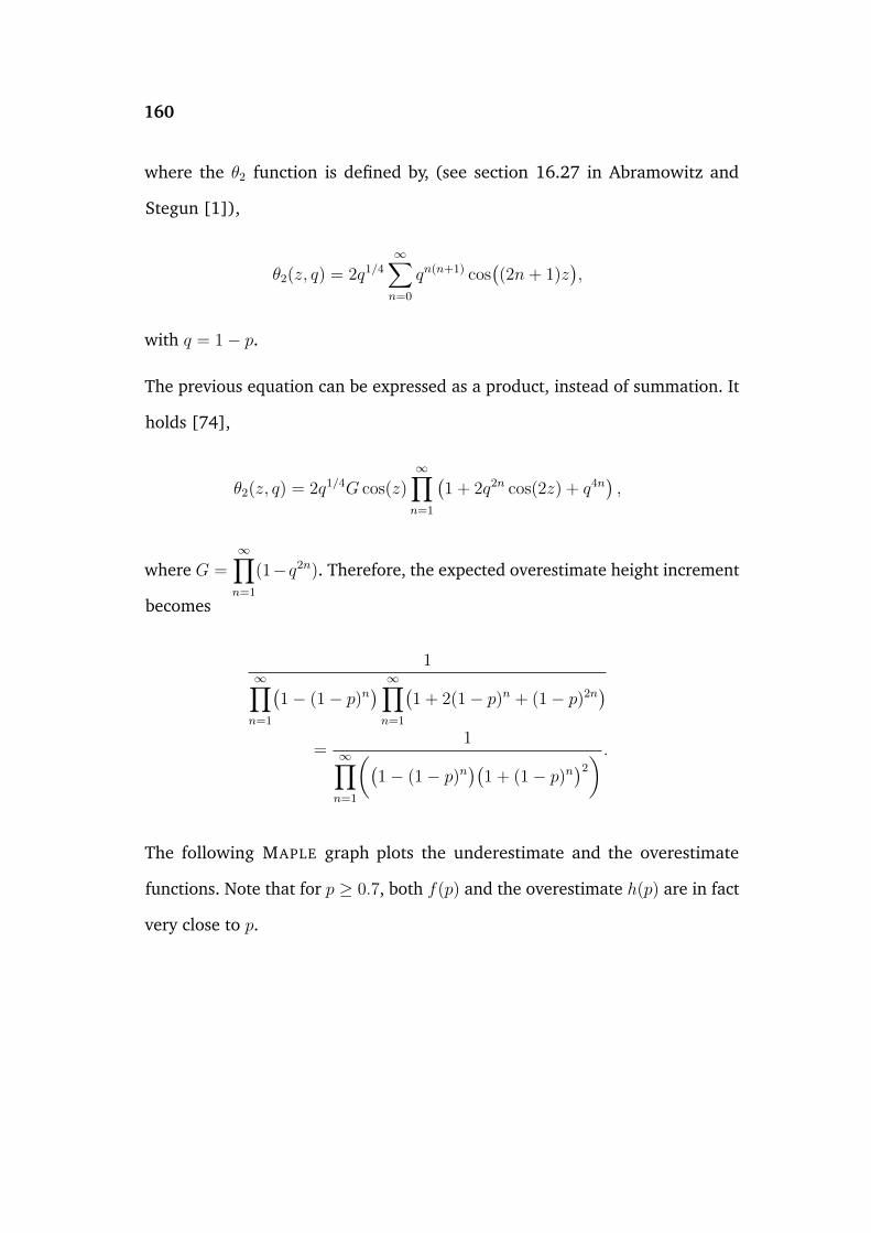
160
where the θ2 function is defined by, (see section 16.27 in Abramowitz and
Stegun [1]),
θ2(z, q) = 2q1/4
∞∑n=0
qn(n+1) cos((2n+ 1)z
),
with q = 1− p.
The previous equation can be expressed as a product, instead of summation. It
holds [74],
θ2(z, q) = 2q1/4G cos(z)∞∏n=1
(1 + 2q2n cos(2z) + q4n
),
where G =∞∏n=1
(1−q2n). Therefore, the expected overestimate height increment
becomes
1∞∏n=1
(1− (1− p)n
) ∞∏n=1
(1 + 2(1− p)n + (1− p)2n
)=
1∞∏n=1
((1− (1− p)n
)(1 + (1− p)n
)2) .
The following MAPLE graph plots the underestimate and the overestimate
functions. Note that for p ≥ 0.7, both f(p) and the overestimate h(p) are in fact
very close to p.
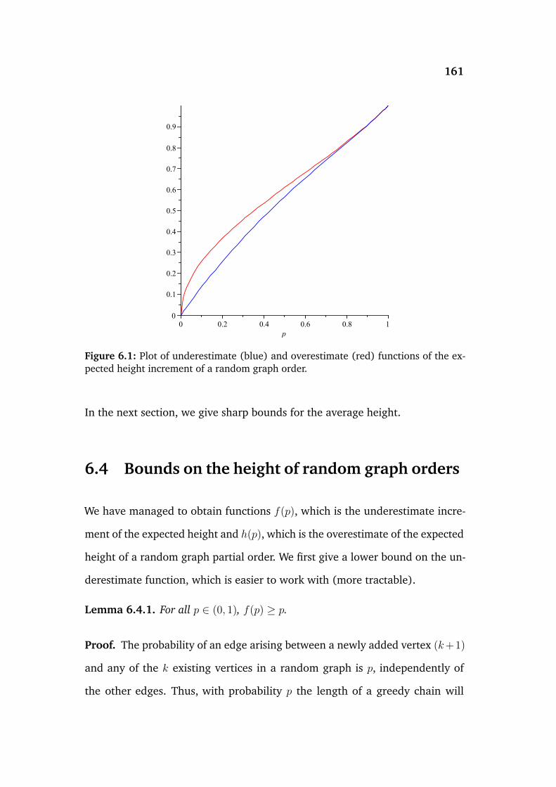
161
Figure 6.1: Plot of underestimate (blue) and overestimate (red) functions of the ex-pected height increment of a random graph order.
In the next section, we give sharp bounds for the average height.
6.4 Bounds on the height of random graph orders
We have managed to obtain functions f(p), which is the underestimate incre-
ment of the expected height and h(p), which is the overestimate of the expected
height of a random graph partial order. We first give a lower bound on the un-
derestimate function, which is easier to work with (more tractable).
Lemma 6.4.1. For all p ∈ (0, 1), f(p) ≥ p.
Proof. The probability of an edge arising between a newly added vertex (k+1)
and any of the k existing vertices in a random graph is p, independently of
the other edges. Thus, with probability p the length of a greedy chain will

162
increase by one and with probability (1− p), the length will remain unchanged.
Thus, the expected increase in the height of a chain is p and the claim follows
immediately.
Here is an upper bound on the overestimate function.
Lemma 6.4.2. It holds that
h(p) ≤ p+(p− 1)2
2− p.
Proof. To obtain an upper bound on
h(p) =1
1 + (1− p) + (1− p)3 + . . .
it is enough to bound below the denominator 1 + (1− p) + (1− p)3 + . . . .
A crude lower bound is 2− p (as all other terms are positive). Thus
h(p) ≤ 1
2− p.
This in turn is
1
2− p=
1
1− (p− 1)= 1 + (p− 1) + (p− 1)2 + . . .
= p+ (p− 1)2 + (p− 1)3 + . . .
= p+(p− 1)2
1− (p− 1)
= p+(p− 1)2
2− p.

163
Collecting more terms, we will be able to obtain a sharper bound in the follow-
ing manner. It holds that
1 + (1− p) + (1− p)3 + . . . > 2− p+ (1− p)3 + . . .+ (1− p)K ,
for a finite number K =m(m− 1)
2, where m ∈ N, so the bound has the
form
1
2− p+m∑j=3
((1− p)
j(j−1)2
) .
Its sharper than the previous one but again infinitely many terms are discarded.
In order to obtain a bound using all terms, note that j(j − 1)/2 ≤ j2 and
1 + (1− p) + (1− p)3 + . . . ≥ (1− p) + (1− p)4 + (1− p)9 + . . . .
The overestimate can be bounded above by another theta function. A sharper
bound is
h(p) ≤ 2
θ3(0, 1− p) + 1,
where the θ3 function is defined [1]
θ3(z, q) = 1 + 2∞∑n=1
qn2
cos(2nz).
Thus, we derived suitable bounds, such that
p ≤ f(p) < h(p) ≤ 2
θ3(0, 1− p) + 1.
164
In the following section, we present bounds on the number of linear exten-
sions.
6.5 Expected number of linear extensions
Here we obtain bounds on the average number of linear extensions of a random
graph order. We start by quoting a useful Theorem from [4],
Theorem 6.5.1 (Alon et al. [4]). Let a random variable Y be geometrically
distributed, i.e. P(Y = k) = pqk−1, for k = 1, 2, . . . . Then,
E(loge(Y )
)=∞∑k=1
loge(k)pqk−1 < µ(p)
≤(1− k(p)
)loge
1/p− k(p)
1− k(p)
< loge1
p= loge
(E(Y )
),
where k(p) is defined as,
k(p) =∞∏k=1
(1− qk),
with q = 1− p.
The following Theorem regarding the expected number of linear extensions is
the main contribution in this Chapter.
Theorem 6.5.2. Let p ∈ (0, 1). The average increment of the natural logarithm
of the number of linear extensions µ(p) =E(loge
(e(P )
))n
is whp. bounded below
by:
µ(p) ≥ − log2 h(p) loge(2)
2.
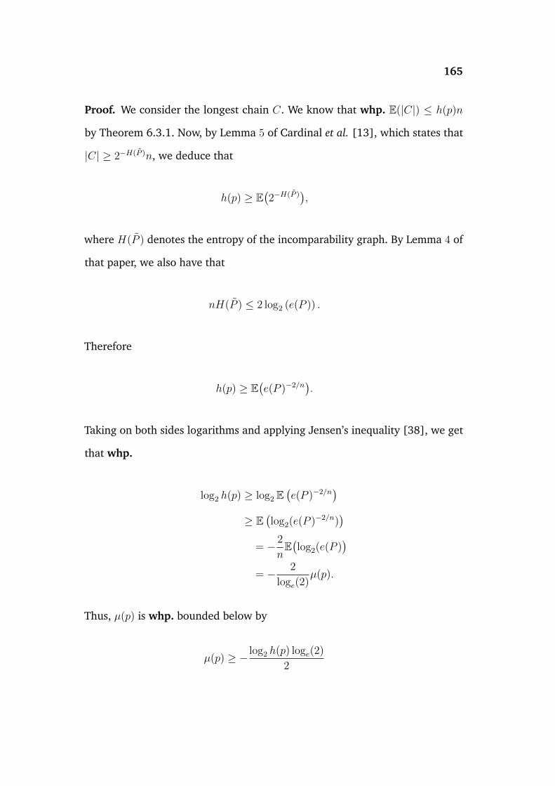
165
Proof. We consider the longest chain C. We know that whp. E(|C|) ≤ h(p)n
by Theorem 6.3.1. Now, by Lemma 5 of Cardinal et al. [13], which states that
|C| ≥ 2−H(P )n, we deduce that
h(p) ≥ E(2−H(P )
),
where H(P ) denotes the entropy of the incomparability graph. By Lemma 4 of
that paper, we also have that
nH(P ) ≤ 2 log2 (e(P )) .
Therefore
h(p) ≥ E(e(P )−2/n
).
Taking on both sides logarithms and applying Jensen’s inequality [38], we get
that whp.
log2 h(p) ≥ log2 E(e(P )−2/n
)≥ E
(log2(e(P )−2/n)
)= − 2
nE(log2(e(P )
)= − 2
loge(2)µ(p).
Thus, µ(p) is whp. bounded below by
µ(p) ≥ − log2 h(p) loge(2)
2
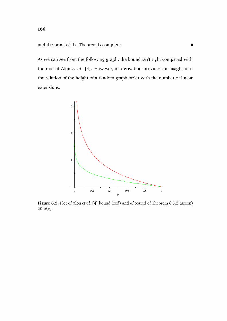
166
and the proof of the Theorem is complete.
As we can see from the following graph, the bound isn’t tight compared with
the one of Alon et al. [4]. However, its derivation provides an insight into
the relation of the height of a random graph order with the number of linear
extensions.
Figure 6.2: Plot of Alon et al. [4] bound (red) and of bound of Theorem 6.5.2 (green)on µ(p).
Chapter 7
Conclusions and future research di-
rections
At the last Chapter of this thesis, the conclusions of the research and possi-
ble future directions are discussed. In the first section, we consider the sort-
ing of partially ordered sets and in the second section, the fast merging of
chains.
7.1 Sorting partially ordered arrays
Central to the analysis of the time complexity of sorting partially ordered sets,
was the number of linear extensions, as a measure of the ‘presortedness’ of
the array. Recall that the quantity log2(n!) is the lower bound of comparisons
needed to sort an array of n keys, with no prior information. In all cases of par-
tially ordered sets considered in Chapter 5, the constant 1/2 log2(e) appeared to
the asymptotic number of comparisons. A future direction to research might be
the sharpening of these results. For example, one might ask, what is the average
number of key exchanges or the computation of exact expected costs.
167
168
Generalising Albert–Frieze argument [3] and using entropy arguments, a new
result was the lower bound on the number of linear extensions of a random
graph order. However, we have seen that it does not directly compete the
bounds of Alon et al. [4], thus there is space for further improvement of this
bound or to derivation of new sharper ones and this might be a suitable topic
for further research.
A different bound on the number of linear extensions of a random interval
order can be derived as follows. By Theorem 5.6.5, one can deduce that whp.,
the size of the longest chain C, is
|C| = 2√n√π.
Using the result |C| ≥ 2−H(P )n from Cardinal et al., as in Theorem 6.5.2, we
have
2√nπ≥ 2−H(P ).
Taking logarithms, a lower bound for the entropy of the incomparability ran-
dom interval graph is,
H(P ) ≥ 1
2log2(n) +O(1).
By the following inequality [13]
nH(P ) ≤ 2 log2
(e(P )
),
169
log2
(e(P )
)is whp. bounded below by
log2
(e(P )
)≥ n
4log2(n) +O(n).
Thus, whp.
log2
(e(P )
)≥ n
4log2(n)
(1 + o(1)
)=
n
4 loge(2)loge(n)
(1 + o(1)
)≈ 0.36n loge(n)
(1 + o(1)
).
Remark 7.1.1. The speed up factor of the derived bound of the number of linear
extensions of a random interval order is 1/4 loge(2) ≈ 0.36 – exactly half of the
constant stated in Corollary 5.6.6. This fact shows that the bound in this Chapter
performs rather poorly, comparing with the results in section 5.6. Note that, with
further information about the entropy, improvement might be possible.
7.2 Merging chains using Shellsort
In the last section, we consider the merging of chains. This problem is anal-
ysed in the paper of Hwang and Lin [32], where an efficient algorithm is
presented.
Here, we discuss some preliminary ideas, that might be worthwhile for further
study. Specifically, we propose the application of Shellsort for the merging of
linearly ordered sets. Shellsort was invented by Donald Shell [66] in 1959
and is based on insertion sort. The algorithm runs from left to right, by com-
170
paring elements at a given gap or increment d ∈ N and exchanging them,
if they are in reverse order, so in the array a1, a2, . . . , an the d subarrays
aj, aj+d, aj+2d, . . ., for j = 1, 2, . . . , d are separately sorted. At the second pass,
Shellsort runs on smaller increment, until after a number of passes, the incre-
ment becomes d = 1. This final insertion sort completes the sorting of the
array.
The sequence of the increments is crucial for the running time of the algorithm,
as the pivot selection is important to Quicksort. Shell [66] proposed the se-
quence⌊n2
⌋,⌊n4
⌋, . . . , 1, which leads to quadratic time. Pratt [57] suggested a
sequence of the form 2a3b < n, where a, b ∈ N, which yields Θ(n log2
2(n))
time.
Incerpi and Sedgewick [36] have shown that there do exist loga(n) increments,
for which the running time of the algorithm is O(n1+ ε√
log2(n) ), with a = 2ε2/8
and ε > 0. Despite the extensive analysis of Shellsort, there are many open
problems, as whether the algorithm can achieve on the average O(n log2(n)
)run-time.
In our problem, Shellsort can be fruitfully applied to merging chains, which
can be done quite fast, using the knowledge of the partial order. Consider two
chains C1 and C2,
C1 = a1 < a2 < . . . < an
C2 = b1 < b2 < . . . < bm.
Starting from a1, with initial increment d = maxn,m, the algorithm sepa-
rately sorts d subarrays. At the second pass, the algorithm iterates from a2 with
171
increment d− 1. The final comparison of the element occupying the location d
with its adjacent key in the position d+1, terminates the merging process.
We illustrate this informal idea, with a simple example. Suppose that we want
to merge the chains C1 = 5, 7, 9, 11, 12 and C2 = 4, 6, 10. We start with
the array 5, 7, 9, 11, 12, 4, 6, 10 and initial increment max5, 3 = 5. Then,
the following subarrays are independently sorted: 5, 4, 7, 6, 9, 10, so at
the end of the first iteration, the array becomes 4, 6, 9, 11, 12, 5, 7, 10. Start-
ing from 6, with increment equal to 4, the algorithm proceeds to the subarrays
6, 5, 9, 7, 11, 10, so we obtain 4, 5, 7, 10, 12, 6, 9, 11. In the same manner,
starting from 7, with gap equal to 3, the subarrays 7, 6, 10, 9, 12, 11 are
sorted, giving 4, 5, 6, 9, 11, 7, 10, 12. Then, the subarrays 9, 7, 12 and 11, 10
are sorted, yielding 4, 5, 6, 7, 10, 9, 11, 12. The final comparison to 10, 9 re-
turns the merged chain. This algorithm took 13 comparisons for the merging
of 8 keys. A different increment sequence might speed up the process, noting
that there are some redundant comparisons, e.g. the comparison of 9, 7 in
the second pass. Its appealing feature is that it merges ‘in-place’, without the
need of auxiliary memory.
Central to the argument is the number of inversions of a permutation of n
distinct keys a1, a2, . . . , an. An inversion is a pair of elements, such that for
i < j, ai > aj. Obviously, an upper bound for the number of inversions is
1+2+. . .+(n−1) =
(n
2
). On the other hand, a sorted array has 0 inversions. In
other words, the number of inversions determine the ‘amount’ of work needed
for the complete sorting. Generally, when one has to merge k chains, with
cardinalities m1,m2, . . . ,mk and∑k
j=1mj = n, an upper bound to the number
172
of inversions is
(n
2
)−
((m1
2
)+
(m2
2
)+ . . .+
(mk
2
)).
Note that this bound corresponds to the case, where the chains are presented
in completely wrong order, e.g. the elements of a chain Cj are greater from the
elements of chains, which lie to its right. In practice, this case occurs rarely, so
the bound can be greatly improved.
The application of Mergesort, as proposed by Cardinal et al. [13] for the merg-
ing of chains completes the sorting in (1 + ε) log2
(e(P )
)+O(n) time – see their
Theorem 3. Cardinal et al. remark in their paper that their Mergesort algorithm
is better than an earlier one of Kahn and Kim [40], provided log2
(e(P )
)is
super–linear. As we have seen in this Chapter, log2
(e(P )
)is linear, thus the
application of Shellsort might constitute an alternative choice for the merging
of chains.
Appendix A
MAPLE Computations
Here is the MAPLE worksheet for the computation of the variance of the num-
ber of key comparisons of dual pivot Quicksort.
> restart;
> f_n(z):= 1/binomial(n, 2)sum(sum(z^2n-i-2f_i-1(z)f_j-i-1(z)
f_n-j(z), j=i+1..n), i=1..n-1);
> diff(f_n(z), z$2);
> subs(z = 1, diff(f_n(z), z$2));
f ′′n(1) =2
n(n− 1)
(n−1∑i=1
n∑j=i+1
(2n− i− 2)2 −n−1∑i=1
n∑j=i+1
(2n− i− 2)
+ 2n−1∑i=1
n∑j=i+1
(2n− i− 2)E(Ci−1,2) + 2n−1∑i=1
n∑j=i+1
(2n− i− 2)E(Cj−i−1,2)
+ 2n−1∑i=1
n∑j=i+1
(2n− i− 2)E(Cn−j,2) + 2n−1∑i=1
n∑j=i+1
E(Ci−1,2)E(Cj−i−1,2)
+ 2n−1∑i=1
n∑j=i+1
E(Ci−1,2)E(Cn−j,2) + 2n−1∑i=1
n∑j=i+1
E(Cj−i−1,2)E(Cn−j,2)
+n−1∑i=1
n∑j=i+1
f ′′i−1(1) +n−1∑i=1
n∑j=i+1
f ′′j−i−1(1) +n−1∑i=1
n∑j=i+1
f ′′n−j(1)
). (A.1)
173
174
The following MAPLE commands compute the sums of Eq. (A.1)
> sum(sum((2n-i-2)^2, j=i+1..n), i=1..n-1);
> sum(sum((2n-i-2), j=i+1..n), i=1..n-1);
> 2(sum(sum((2n-i-2)(2iharmonic(i-1)-4(i-1)), j = i+1..n), i = 1..n-1));
> simplify(%);
> 2(sum(sum((2n-i-2)((2(j-i))harmonic(j-i-1)-4(j-i-1)),
j=i+1..n), i=1..n-1));
> sum(4 n harmonic(k)(k+i+1)-4nharmonic(k)i-2iharmonic(k)(k+i+1)
+2harmonic(k) i^2-4harmonic(k)(k+i+1)+4iharmonic(k), k=0..n-i-1);
> 2(sum(3n-3i+2nharmonic(n-i)(n-i)^2 -iharmonic(n-i)(n-i)
+2nharmonic(n-i)(n-i)-(3(n-i))n+(3/2(n-i))i-iharmonic(n-i)(n-i)^2
-2harmonic(n-i) (n-i)^2
+(1/2)i(n-i)^2-2harmonic(n-i)(n-i)-n (n-i)^2+(n-i)^2, i=1..n-1));
> 2(sum(4nharmonic(j)(n-j)^2-5n^2harmonic(j)(n-j)-2nharmonic(j)
+(n-j)harmonic(j)n+(2(n-j))harmonic(j)-(n-j)^2
harmonic(j)+2n^3 harmonic(j)-(n-j)^3 harmonic(j), j=1..n-1));
> sum((2(k+1))harmonic(k)-4k, k = 0..n-i-1);
> 2(sum((2iharmonic(i-1)-4(i-1))(2binomial(n-i+1, 2)
harmonic(n-i)+(n-i-5(n-i)^2)(1/2)), i=1..n-1));
> sum((8(n-k))binomial(k+1, 2)harmonic(k), k=1..n-1);
> sum(8binomial(k+1, 2)harmonic(k), k=1..n-1);
175
Using these results, the second-order derivative evaluated at 1 is given recur-
sively by:
f ′′n(1) = 2(n+ 1)(n+ 2)(H2n −H(2)
n )−Hn
(17
3n2 +
47
3n+ 6
)+
209
36n2
+731
36n+
13
6+
6
n(n− 1)
n−1∑i=1
(n− i)f ′′i−1(1). (A.2)
The MAPLE input for the solution of the recurrence is as follows
> f’’_n(1)=2 (harmonic(n))^2 n^2-17/3 harmonic(n) n^2+209/36 n^2
-2 harmonic(n,2) n^2+731/36 n-6 harmonic(n,2) n-47/3 harmonic(n) n
+6 (harmonic(n))^2 n+4 (harmonic(n))^2-4 harmonic(n,2)-6 harmonic(n)
+13/6+6/(n(n-1))sum((n-i)f’’_i-1(1), i=1..n-1);
> binomial(n, 2)f’’_n(1);
> binomial(n+1, 2)f’’_n+1(1)- binomial(n, 2)f’’_n(1);
> binomial(n+2, 2)f’’_n+2(1)-2binomial(n+1, 2)f’’_n+1(1)
+ binomial(n, 2)f’’_n(1);
The output of these commands gives the second–order difference
∆2
(n
2
)f ′′n(1) = 12(n+ 1)(n+ 2)(H2
n −H(2)n )−Hn(20n2 + 32n− 12)
+ 17n2 + 37n+ 3f ′′n(1) (A.3)
and after standard manipulations of Eq. (A.3), (recall subsection 4.1.1), the
solution of the recurrence is
f ′′n(1) = 4(n+ 1)2(H2n+1 −H
(2)n+1)− 4Hn+1(n+ 1)(4n+ 3) + 23n2 + 33n+ 12.
Bibliography
[1] Abramowitz, M. and Stegun, I. A. (1972) “Handbook of Mathematical
Functions with Formulas, Graphs, and Mathematical Tables.” Dover Publi-
cations.
[2] Albacea, E. A. (2012) “Average-case analysis of Leapfrogging samplesort.”
Philipp. Sci. Lett. 5 (1): 14–16.
[3] Albert, M. and Frieze A. (1989) “Random graph orders.” Order 6 (1):
19–30.
[4] Alon, N., Bollobás, B., Brightwell, G. and Janson, S. (1994) “Linear Exten-
sions of a Random Partial Order.” Ann. Appl. Probab. 4 (1): 108–123.
[5] Bell, D. A. (1958) “The Principles of Sorting.” Comput. J. 1 (2): 71–77.
[6] Bentley, J. L. (2000) “Programming Pearls.” Addison-Wesley Publishing,
second edition.
[7] Bentley, J. L. and McIlroy, M. D. (1993) “Engineering a Sort Function.”
Software Pract. Exper. 23 (11): 1249–1265.
[8] Billingsley, P. (2012) “Probability and measure.” John Wiley & So., third
edition.
[9] Boyce, W. E., DiPrima, R. C. (2001) “Elementary Differential Equations
and Boundary Value Problems.” John Wiley & So., seventh edition.
176
177
[10] Brightwell, G. (1993) “Models of Random Partial Orders.” Surveys in Com-
binatorics, Cambridge University Press.
[11] Brightwell, G., Prömel, H. J. and Steger, A. (1996) “The Average Number
of Linear Extensions of a Partial Order.” J. Comb. Theory, Ser. A 73 (2):
193–206.
[12] Brightwell, G. (1992) “Random k-dimensional orders: Width and number
of Linear extensions.” Order 9 (4): 333–342.
[13] Cardinal, J., Fiorini, S., Joret, G., Jungers, R. and Munro, I. (2010) “Sort-
ing under partial information (without the Ellipsoid algorithm).” STOC’
10 Proceedings of the 42nd ACM symposium on Theory of computing,
359–368.
[14] Chern, H. H., Hwang, H. K. and Tsai, T. H. (2002) “An asymptotic theory
for Cauchy–Euler differential equations with applications to the analysis of
algorithms.” J. Algorithm. 44 (1): 177–225.
[15] Cormen, T. H. Leiserson, C. E. Rivest, R. L. and Stein, C. (2001) “Intro-
duction to Algorithms.” M.I.T. Press, second edition.
[16] Cover, T. M. and Thomas, J. A. (1991) “Elements of Information Theory.”
John Wiley & So., second edition.
[17] Dilworth, R. P. (1950) “A Decomposition Theorem for Partially Ordered
Sets.” Ann. Math. 51 (1): 161–166.
[18] Durand, M. (2003) “Asymptotic analysis of an optimized quicksort algo-
rithm.” Inform. Process. Lett. 85 (2): 73–77.
178
[19] van Emden, M. H. (1970) “Increasing the efficiency of Quicksort.” Comm.
ACM. 13 (9): 563–567.
[20] Erkiö, H. (1984) “The Worst Case Permutation for Median-of-Three Quick-
sort.” Comput. J. 27 (3): 276–277.
[21] Feller, W. (1957) “An Introduction to Probability Theory and its Applica-
tions, Vol. II.” John Wiley & So., first edition.
[22] Fill, J. A. and Janson, S. (2002) “Quicksort Asymptotics.” J. Algorithm. 44
(1): 4–28.
[23] Fishburn, P. (1985) “Interval Orders and Interval Graphs.” Discrete Math.
55 (2): 135–149.
[24] Frazer, W. D. and McKellar, A. C. (1970) “Samplesort: A Sampling Ap-
proach to minimal storage Tree Sorting.” J. ACM. 17 (3): 496–507.
[25] Fredman, M. L. (1976) “How good is the information theory bound in
sorting?” Theor. Comput. Sci. 1 (4): 355–361.
[26] Graham, R. L., Knuth, D. E. and Patashnik, O. (1994) “Concrete Mathe-
matics: A Foundation for Computer Science.” Addison-Wesley Publishing,
second edition.
[27] Hennequin, P. (1989) “Combinatorial analysis of quicksort algorithm.”
RAIRO Theor. Inform. Appl. 23 (3): 317–333.
[28] Hennequin, P. (1991) “Analyse en moyenne d’algorithmes, tri rapide et
arbres de recherche.” Ph.D. thesis. École Polytechnique.
[29] Hoare, C. A. R. (1961) “Algorithm 63: Partition, Algorithm 64: Quicksort,
and Algorithm 65: Find.” Comm. ACM. 4 (7): 321–322.
179
[30] Hoare, C. A. R. (1962) “Quicksort.” Comput. J. 5 (1): 10–15.
[31] Hou, S. H. and Hou, E. (2008) “Triangular Factors of the Inverse of Van-
dermonde Matrices.” Proceedings of the International MultiConference of
Engineers and Computer Scientists. Vol. II, IMECS.
[32] Hwang, F. K. and Lin, S. (1972) “A simple algorithm for merging two
disjoint linearly ordered sets.” SIAM J. Comput. 1 (1): 31–39.
[33] Iliopoulos, V. and Penman, D. B. (2010) “Variance of the number of Com-
parisons of Randomised Quicksort.” arXiv: 1006.4063.
[34] Iliopoulos, V. and Penman, D. B. (2012) “Dual Pivot Quicksort.” Discrete
Math. Algorithm. Appl. 4 (3): 1250041.
[35] Iliopoulos, V. (2013) “Quicksorting on multiple pivots and a Vandermonde
matrix.” Seminar in the Department of Mathematical Sciences, University
of Essex.
[36] Incerpi, J. and Sedgewick, R. (1985) “Improved Upper Bounds on Shellsort.”
J. Comput. Syst. Sci. 31 (2): 210–224.
[37] Janson, S., Łuczak, T. and Rucinski, A. (2000) “Random Graphs.” John
Wiley & So., first edition.
[38] Jensen, J. L. W. V. (1906) “Sur les fonctions convexes et les inégalités entre
les valeurs moyennes.” Acta Math. 30 (1): 175–193.
[39] Justicz, J., Scheinerman, E. and Winkler, P. (1990) “Random Intervals.”
Amer. Math. Monthly 97 (10): 881–889.

180
[40] Kahn, J. and Kim, J. H. (1992) “Entropy and sorting.” STOC’ 92 Pro-
ceedings of the 24th annual ACM symposium on Theory of computing,
178–187.
[41] Kislitsyn, S. S. (1968) “A finite partially ordered set and its corresponding
set of permutations.” Mat. Zametki 4 (5): 511–518.
[42] Kleitman, D. J. and Rothschild, B. L. (1975) “Asymptotic enumeration of
partial orders on a finite set.” Trans. Amer. Math. Soc. 205: 205–220.
[43] Knessl, C. and Szpankowski, W. (1999) “Quicksort algorithm again revis-
ited.” Discrete Math. Theor. Comput. Sci. 3 (2): 43–64.
[44] Knuth, D. E. (1997) “The Art of Computer Programming, Vol. I: Fundamen-
tal Algorithms.” Addison-Wesley Publishing, third edition.
[45] Knuth, D. E. (1997) “The Art of Computer Programming, Vol. II: Seminu-
merical Algorithms.” Addison-Wesley Publishing, second edition.
[46] Knuth, D. E. (1998) “The Art of Computer Programming, Vol. III: Sorting
and Searching.” Addison-Wesley Publishing, second edition.
[47] Körner, J. (1973) “Coding of an Information source having ambiguous
alphabet and the entropy of graphs.” Proceedings of the 6th Prague Con-
ference on Information Theory, 411–425.
[48] Mahmoud, H. M. (2010) “Distributional analysis of swaps in Quick Select.”
Theor. Comput. Sci. 411 (16-18): 1763–1769.
[49] Mahmoud, H. M. (2000) “Sorting: A Distribution Theory.” John Wiley &
So., first edition.
181
[50] McDiarmid, C. J. H. and Hayward, R. B. (1996) “Large Deviations for
Quicksort.” J. Algorithm. 21 (3): 476–507.
[51] McDiarmid, C. J. H. (2013) “Quicksort and Large Deviations.” Mathemat-
ical and Engineering Methods in Computer Science, Lecture Notes in
Computer Science 7721: 43–52.
[52] McDiarmid, C. J. H. (2013) Personal Communications.
[53] McEliece, R. (2002) “The theory of Information and Coding: A Mathemati-
cal Framework for Communication.” University Cambridge Press, second
edition.
[54] Mitzenmacher, M. and Upfal, E. (2005) “Probability and Computing: Ran-
domized Algorithms and Probabilistic Analysis.” Cambridge University
Press.
[55] Mizoi, T. and Osaki, S. (1996) “Probabilistic Analysis of Time Complexity
of Quicksort.” Electron. Comm. Jpn. Pt. III 79 (3): 34–42.
[56] Neggers, J. and Kim, H. S. (1998) “Basic Posets.” World Scientific Publish-
ing.
[57] Pratt, V. (1979) “Shellsort and Sorting Networks.” Ph.D. thesis. Garland
Publishing.
[58] Régnier, M. (1989) “A limiting distribution for Quicksort.” RAIRO Theor.
Inform. Appl. 23 (3): 335–343.
[59] Rösler, U. (1991) “A Limit Theorem for Quicksort.” RAIRO Theor. Inform.
Appl. 25 (1): 85–100.
182
[60] Rousseeuw, P. J. and Bassett, G. W. (1990) “The remedian: A robust aver-
aging method for large data sets.” J. Am. Statist. Assoc. 85 (409): 97–104.
[61] Sabuwala, A. H. and De Leon, D. (2011) “Particular solution to the Euler-
Cauchy equation with polynomial non-homogeneities.” Discret. Contin.
Dyn. S. 2011: 1271–1278.
[62] Scowen, R. S. (1965) “Algorithm 271: Quickersort.” Comm. ACM. 8 (11):
669–670.
[63] Sedgewick, R. (1980) “Quicksort.” Ph.D. thesis. Garland Publishing.
[64] Sedgewick, R. (1977) “Quicksort with Equal Keys.” SIAM J. Comput. 6
(2): 240–267.
[65] Shannon, C. E. (1948) “A Mathematical Theory of Communication.” Bell
Syst. Tech. J. 27 (3): 379–423.
[66] Shell, D. L. (1959) “A High-Speed Sorting Procedure.” Comm. ACM. 2 (7):
30–32.
[67] Simonyi, G. (1995) “Graph Entropy: A Survey.” In Combinatorial Opti-
mization (Ed. W. Cook, L. Lovász, and P. Seymour). DIMACS Series in
Discrete Mathematics and Theoretical Computer Science. Amer. Math.
Soc., 399–441.
[68] Singleton, R. C. (1969) “Algorithm 347: An efficient algorithm for sorting
with minimal storage [M1].” Comm. ACM. 12 (3): 185–186.
[69] Skiena, S. S. (2008) “The algorithm design manual.” Springer, second
edition.
183
[70] Spieß, J. (1990) “Some Identities involving Harmonic numbers.” Math.
Comp. 55 (192): 839–863.
[71] Trotter, W. (1997) “New perspectives of Interval Orders and Interval Graphs.”
Surveys in Combinatorics, Cambridge University Press.
[72] Tukey, J. W. (1978) “The ninther, a technique for low-effort robust (resis-
tant) location in large samples.” In Contributions to Survey Sampling and
Applied Statistics in Honor of H. O. Hartley, Ed. by H. A. David. 251–258,
Academic Press.
[73] Turner, L. R. (1966) “Inverse of the Vandermonde Matrix with Applications.”
National Aeronautics and Space Administration, technical note D-3547.
[74] Whittaker, E. T. and Watson, G. N. (1996) “A Course of Modern Analysis.”
Cambridge University Press, fourth edition.


