The R Journal is a peer-reviewed publication of the RFoundation for Statistical Computing. Communicationsregarding this publication should be addressed to theeditors. All articles are licensed under the Creative
Commons Attribution 4.0 International license (CC BY 4.0,http://creativecommons.org/licenses/by/4.0/).
Prospective authors will find detailed and up-to-datesubmission instructions on the Journal’s homepage.
Editor-in-Chief:Norman Matloff, University of California, Davis, USA
Executive editors:Dianne Cook, Monash University, Australia
Michael Kane, Yale University, USAJohn Verzani, City University of New York, USA
The editorial board and I are pleased to present the latst issue of the R Journal.We apologize that this issue has been so late in publication. As this is my first issue as
Editor-in-Chief, I must personally thank Roger Bivand and John Verzani, the two previousEiCs, for their guidance in the technical aspects of putting an issue together.
The good news, though, is that publication should be much more timely in the future,due to improved internal technical documentation and the hiring of the journal’s first-evereditorial assistants, Stephanie Kobakian and Mitchell O’Hara-Wild. We are thankful to theR Consortium for a grant supporting the assistants (https://rjpilot.netlify.com).
This issue is chock full of interesting papers, many of them on intriguing, unusual topics.For those of us whose connection to R goes back to the old S days, it is quite gratifying tosee the wide diversity of application areas in which R has been found productive.
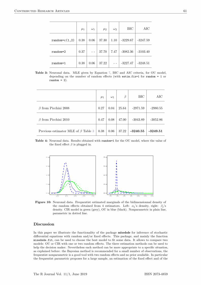
Regular readers of this journal are aware of a change in policy that began January 2017,under which we are moving away from a paradigm in which a typical article is merely anextended user’s manual for the author’s R package.
To be sure, most articles will continue to be tied to specific packages. But we hopefor broader coverage, and even the package-specific articles should emphasize aspects suchas technical challenges the package needed to overcome, how it compares in features andperformance to similar packages, and so on. As described in the announcement:
Short introductions to contributed R packages that are already available onCRAN or Bioconductor, and going beyond package vignettes in aiming to providebroader context and to attract a wider readership than package users. Authorsneed to make a strong case for such introductions, based for example on noveltyin implementation and use of R, or the introduction of new data structuresrepresenting general architectures that invite re-use.
Clearly, there is some subjectivity in assessing these criteria, and views will vary fromone handling editor to the next. But this is the current aim of the journal, so please keep itin mind in your submissions.
We wish the journal to further evolve in two more senses:
• In 2016, the American Statistical Assocation released a dramatic policy statement,seriously questioning the general usefulness and propriety of p-values. Though thestatement did not call for a ban on the practice, it did have a strong theme thatp-values should be used more carefully and less often. Many of us, of course, hadbeen advocating a move away from p-values for years. We wish authors of futuresubmissions to the journal to be mindful of the ASA policy statement. We hope forreduced emphasis on hypothesis testing, and in articles that do include testing, properconsideration of power calculation.
• In the interest of reproducibility—a requirement already imposed by the journal onarticle submissions—we will require that any real datasets used as examples in anarticle must be provided. Note that this will mean that datasets with privacy issues ordatasets of extremely large size should not be used in an article.
Finally, we note our deep appreciation for the anonymous reviewers. A journal is only asgood as its reviewers, and most reviews are quite thoughtful and useful. If a handling editorsolicits your review for a paper, please make some time for it. And if you must decline therequest, a reply to that effect would be quite helpful; don’t just discard the editor’s e-mailmessage. The handling editors are quite busy, and it is unfair to both them and the authorsto have the editors wait until they must conclude you will not reply, causing unnecessarydelay.
Matching with Clustered Data: theCMatching Package in Rby Massimo Cannas and Bruno Arpino
Abstract Matching is a well known technique to balance covariates distribution between treatedand control units in non-experimental studies. In many fields, clustered data are a very commonoccurrence in the analysis of observational data and the clustering can add potentially interestinginformation. Matching algorithms should be adapted to properly exploit the hierarchical structure.In this article we present the CMatching package implementing matching algorithms for clustereddata. The package provides functions for obtaining a matched dataset along with estimates of mostcommon parameters of interest and model-based standard errors. A propensity score matchinganalysis, relating math proficiency with homework completion for students belonging to differentschools (based on the NELS-88 data), illustrates in detail the use of the algorithms.
Background
Causal inference with observational data usually requires a preliminary stage of analysis correspondingto the design stage of an experimental study. The aim of this preliminary stage is to reducethe imbalance in covariates distribution across treated and untreated units due the non-randomassignment of treatment before estimating the parameters of interest. Matching estimators are widelyused for this task (Stuart, 2010). Matching can be done directly on the covariates (multivariatematching) or on the propensity score (Rosenbaum and Rubin, 1983). The latter is defined as theprobability of the treatment given the covariates value and it has a central role for the estimationof causal effects. In fact, the propensity score is a one dimensional summary of the covariates andthus it mitigates the difficulty of matching observations in high dimensional spaces. Propensityscore methods have flourished and several techniques are now well established both in theory and inpractice, including stratification on the propensity score, propensity score weighting (PSW), andpropensity score matching (PSM).
Whilst the implementation of matching techniques with unstructured data has became a standardtool for researchers in several fields (Imbens and Rubin, 2016), the increasing availability of clustered(nested, hierarchical) observational data poses new challenges. In a clustered observational studyindividuals are partitioned into clusters and the treatment is non-randomly assigned in each cluster sothat confounders may exist both at the individual and at the cluster level. Note that this frameworkis different from clustered observational data where a treatment is non-randomly assigned for allunits in the cluster, for which an optimal matching strategy has been suggested by Zubizarretaand Keele (2017). Such nested data structures are ubiquitous in the health and social scienceswhere patients are naturally clustered in hospitals and students in schools, just to make two notableexamples. If relevant confounders are observed at both levels then a standard analysis, adjusting forall confounders, seems reasonable. However, when only the cluster label — but not the cluster levelvariables — is observed there is not a straightforward strategy to exploit the information on theclustering. Intuitively, the researcher having a strong belief on the importance of the cluster levelconfounders may adopt a ’within-cluster ’ matching strategy. On the other extreme, a researcher maydecide to ignore the clustering by using only the pooled data. It is important to note that this poolingstrategy implicitly assumes that cluster level variables are not important confounders. Indeed, therehave been a few proposals to adapt PSW and PSM to clustered data, see Cafri et al. (2018) for areview. Li et al. (2013) proposed several propensity score weighting algorithms for clustered datashowing, both analytically and by simulation, that they reduce the bias of causal effects estimatorswhen "clusters matter," that is, when cluster level covariates are important confounders. In thePSM context, Arpino and Mealli (2011) proposed to account for the clustering in the estimation ofthe propensity score via multilevel models. Recently, Rickles and Seltzer (2014) and Arpino andCannas (2016) proposed caliper matching algorithms to perform PSM with clustered data. As wewill discuss shortly, these algorithms can be used not only for PSM but also in the more generalcontext of multivariate matching.
In the remaining of this paper, after reviewing the basic ideas underlying matching estimators,we briefly describe the available packages for matching in the R environment. Then, we describe thealgorithms for matching with clustered data proposed by Arpino and Cannas (2016) and we presentthe package CMatching implementing these algorithms. The applicability of these algorithms is verybroad and refers to all situations where cluster-level data are present (in medicine, epidemiology,economics, etc.). A section is devoted to illustrate the use of the package on data about studentsand schools, which is a common significant occurrence of clustered data.
A list of the most important packages for matching available for R users is shown in Table 1. TheMatching package, which is required to run CMatching, is a remarkably complete package offeringseveral matching options. Matching implements many greedy matching algorithms including geneticmatching (Diamond and Sekhon, 2013). It also contains a general MatchBalance function to measurepre- and post-matching balance with a large suite of diagnostics. As for optimal matching, there arededicated packages like designmatch and optmatch. The latter can also be called from MatchIT, ageneral purpose package implementing also the Coarsened Exact Matching approach of Iacus et al.(2011). Full matching is a particular form of optimal matching implemented by quickmatch withseveral custom options.
Package Description Reference
Matching Greedy matching and balance analysis Sekhon (2011)
MatchIT Greedy matching and balance analysis Iacus et al. (2011)
optmatch Optimal matching Hansen and Klopfer (2006)
quickmatch Generalized full matching Savje et al. (2018)
designmatch Optimal matching and designs Zubizarreta et al. (2018)
Table 1: General purpose packages available from CRAN implementing matching algorithms.The list is not exhaustive as there are several packages covering specialized matchingroutines: a list can be found at http://www.biostat.jhsph.edu/ estuart/propensityscore-software.html.
At the time of writing none of the packages described above offers specific routines for clustereddata. The CMatching package fills this important gap implementing the algorithms for matchingclustered data described in the next section.
Matching clustered data
Let us consider a clustered data structure D “ tyij ,xij , tiju, i “ 1, ¨ ¨ ¨nj , j “ 1, ¨ ¨ ¨ J . Forobservation i in cluster j we observe a vector of covariates X and a binary variable T specifyingthe treatment status of each observation. Here n “
ř
nj is the total number of observations and Jis the number of clusters in the data. We observe also a response variable Y whose average valuewe are willing to compare across treated and untreated units. A matching algorithm assigns a(possibly empty) subset of control units to each treated unit. The assignment is made with the aimof minimizing a loss function, typically expressed in terms of covariates distance between treatedand untreated units. Matching algorithms can be classified as greedy or optimal depending whetherthe cost function is minimized locally or globally, respectively. Optimal matching algorithms are notaffected by the order of the units being matched so they can reach the global optimum, but they aretypically more computer-intensive than greedy algorithms proceedings step by step. To bound thepossibility of bad matches in greedy matching, it is customary to define a maximum distance fortwo units to be matched, i.e., a caliper, which is usually expressed in standard deviation units of thecovariates (or of the propensity score). one covariate.
A greedy matching procedure can then be articulated in the following steps:
1. fix the caliper;2. match each treated with control unit(s) at minimum covariates distance (provided that distance
3. measure the residual covariates’ imbalance in the matched dataset and count the number ofunmatched units (drops);
4. carefully consider both the balance and the number of drops: if they are satisfactory thenproceed to the outcome analysis; otherwise stop or revise previous steps.
If matching proves successful in adjusting covariates, the researcher can proceed to outcomeanalysis where the causal estimand of interest is estimated from the matched data using a varietyof techniques (Ho et al., 2007). On the other hand, if the procedure gives either an unsatisfactorybalance or an excessive number of unmatched units, the investigator may try to modify some aspectsof the procedure (e.g., the caliper, the way the distance is calculated).
Conceptually, the same procedure can be used also for hierarchical data. Indeed, it is notatypical to find analysis ignoring the clustering and pooling together all units. A pooling strategyimplicitly assumes that the clustering is not relevant. However, in several cases the clusteringdoes matter, that is, the researcher can hypothesize or suspect that some important cluster-levelconfounders are unobserved. In this case, the information on the cluster labels can be exploited inat least two ways: i) forcing the matching to be implemented within-cluster only; ii) performing apreferential within-cluster matching, an intermediate approach between the two extremes of pooledand within-cluster matching (Arpino and Cannas, 2016). A within-cluster matching can be obtainedby modifying step 2 above in the following way:
2’ match each treated with the control unit(s) in group j at minimum covariate distance (providedthat distance < caliper).
This procedure may result in a large number of unmatched units (drops) so it increases the riskof substantial bias due to incomplete matching (Rosenbaum and Rubin, 1985), in particular whenthe clusters are small. This particular bias arises when a matched subset is not representative ofthe original population of treated units because of several non random drops. Even in the absenceof bias due to incomplete matching, a high number of drops reduces the original sample size withpossible negative consequences in terms of higher standard errors.
It is possible to profit as much as possible of the the exact balance of (unobserved) cluster-levelcovariates by first matching within clusters and then recovering some unmatched treated units ina second stage. This leads to the preferential within-cluster matching, which can be obtained bymodifying step 2 above in the following way:
2” a) match each treated with the control units(s) in group j at minimum covariate distance(distance < caliper);
2” b) match each unmatched treated unit from previous step with the control unit(s) at minimumcovariate distance in some group different from j (provided that distance < caliper).
Now consider the outcome variable Y . We can define for each unit potential outcomes Y 1, Y 0as the outcome we would observe under assignment to the treatment and control group, respectively(Holland, 1986). Causal estimands of interest are the Average Treatment effect: ATE “ ErY 1´ Y 0sor, more often, the Average Treatment effect on the treated: ATT “ TErY 1´ Y 0s. Given that aunit is either assigned to the treatment or control group it is not possible to directly observe theindividual causal effect on each unit; we have Y “ T ¨ Y 1` p1´ T q ¨ Y 0. In a randomized study T isindependent of pY 0,Y 1q so, for k “ 0, 1, we have
EpY kq “ EpY k |T “ kq “ EpY |T “ kq
which can be estimated from the observed data. In a observational study, matching can be used tobalance covariates across treated and control units and then the previous relation can be exploited toimpute the unobserved potential outcomes from the matched dataset. In our clustered data context,after the matched dataset has been created using one of the algorithms above, the ATT and itsstandard error can be estimated using a simple regression model:
Yij “ αj ` Tijβ (1)
that is, a linear regression model with clustered standard errors to take into account within-cluster dependence in the outcome (Arpino and Cannas, 2016). The resulting ATT estimate isthe difference of outcome means across treated and controls, i.e., zATT :“ meanpY |T “ 1q ´meanpY |T “ 0q, computed on the matched data. Standard errors are calculated using the clusterbootstrapping method for estimating variance-covariance matrices proposed by Cameron et al. (2011)and implemented in the package multiwayvcov. In general, calculating standard errors for PSM inclustered observational studies is a difficult problem requiring prudence from the researcher. Whileclose formulae exist for weighting estimators (Li et al., 2013), standard error estimation after PSM
matching relies upon approximation (Cafri et al., 2018), modelling assumption (Arpino and Cannas,2016), or simulation (Rickles and Seltzer, 2014).
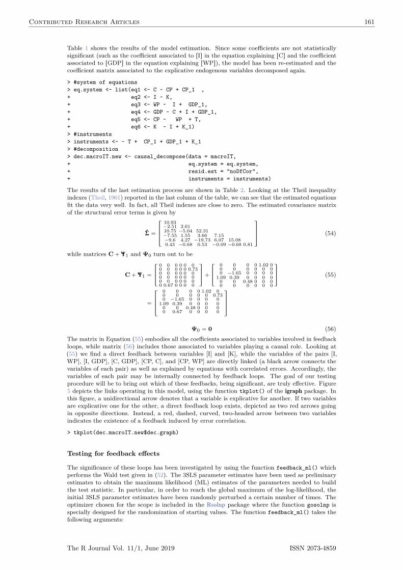
Multisets and matching output
In this section we briefly detail the two routines in the CMatching package. Multisets are usefulto compactly describe pseudo code so we recall some definitions and basic properties herein. Amultiset is a pair tU ,mu where U is a given set, usually called universe, and m : x Ñ NY t0u isthe multiplicity function assigning each x P U its frequency in U . Both the summation symboland union symbols are used to manipulate multisets and they have different meanings: if A andB are multisets then C ” AYB is defined by mCpxq “ maxpmApxq,mBpxqq, while C ” A`Bis defined by mCpxq “ mApxq `mBpxq. For example if A ” t1, 2, 2u and B ” t1, 2, 3u thenAYB ” t1, 2, 2, 3u, A`B ” t1, 1, 2, 2, 2, 3u. In our framework U is the set of observations indexesand thus m gives information about the number of times a given observation occurred in the matcheddataset. Multisets then allow to naturally represent multiple matches arising from matching withreplacement. When using multiset notation to describe the output of a matching algorithm, we areimplicitly overlooking the fact that the output of a matching algorithm is richer as it also brings outthe pairings, i.e., the associations between matched treated and untreated observations. However,it can be noted that this pairing is not relevant for calculating common estimates or commonbalance measures (e.g., the ATT), as they are invariant to permutations of the labels of the matchedobservations.
The routines MatchW and MatchPW
We denote with Wi and W i the sets of treated observations matched within clusters and unmatchedwithin clusters, respectively. In Algorithms 1 and 2, the summation symbol p
ř
q denotes multisetsum.
# Algorithm 1 : within´c l u s t e r matchingprocedure MatchW( data )
f i nd Wi f o r each i us ing Match func t i onM :=
ř
iWi # f ind matched with inmdata := data [M] # ex t r a c t s matched datai f data conta in s outcome va r i ab l e Y:
e s t imate zATT and sdpzATT q from model on mdatae l s e zATT < sdpzATT q < NULLreturn mdata , zATT and sdpzATT q
# Algorithm 2 : f o r p r e f e r e n t i a l within´c l u s t e r matchingProcedure MatchPW( data )
f i nd Wi and W i f o r each i us ing Match func t i onB := Match (
ř
iW i Y a l l c on t r o l s )M :=
ř
iWi `Bmdata := data [M] # ex t r a c t s matched datai f data conta in s outcome va r i ab l e Y:
e s t imate zATT and sdpzATT q from model on mdatae l s e zATT < sdpzATT q < NULLreturn mdata , zATT and sdpATT q
In the first two lines, common to both algorithms, the Match function is repeatedly run toproduce the matched-within subsets Mi i “, ..., J . Then, in Algorithm 1 the sum of the Mi in line3 gives the matched subset M . Algorithm 2 is similar but after finding the Mi’s an "additional"subset B is found by recovering some unmatched units (line 3) and then combined to give the finalmatched dataset. If a response variable Y was included the output of both algorithms also containsan estimate of the ATT (default, but the user can choose also other estimands) and its standarderror.
Functions in the CMatching package
CMatching can be freely downloaded from CRAN repository and it contains the functions listedin Table 2. The main function CMatch performs within-cluster and preferential within-cluster
The R Journal Vol. 11/1, June 2019 ISSN 2073-4859
Contributed Research Articles 11
matching via subfunctions MatchW and MatchPW, respectively. The output of the main function canbe passed to functions CMatchBalance and summary to provide summaries of covariates balance andother characteristics of the matched dataset. CMatch exploits the Match function (see Matching)implementing matching for unstructured data. Given a covariate X and a binary treatment T, the callMatch(X,T,...) gives the set of indexes of matched treated and matched control units. The CMatchfunction has the same arguments plus the optional arguments G (specifying the cluster variable)and type to choose between within-cluster matching or preferential-within-cluster matching. Wehighlight that we chose to frame the CMatch in the Match function style so that Matching users caneasily implement PSM with clustered data in a familiar setting.
Function Description Input Output
CMatch Match X, T , G A matched dataset
MatchW Match within X, T , G A matched dataset
MatchPW Match preferentially within X, T , G A matched dataset
summary.Match S3 method for CMatch objects A matched dataset General summaries
CMatchBalance Balance analysis A matched dataset Balance summaries
Table 2: Main input and output of functions in CMatching package.
1 3
2 4
9
10
6 8
5 7
Pooledasam=173
1 3
2 4
9
10
6 8
5 7
Withinasam=115
1 3
2 4
9
10
6 8
5 7
Preferential-withinasam=216
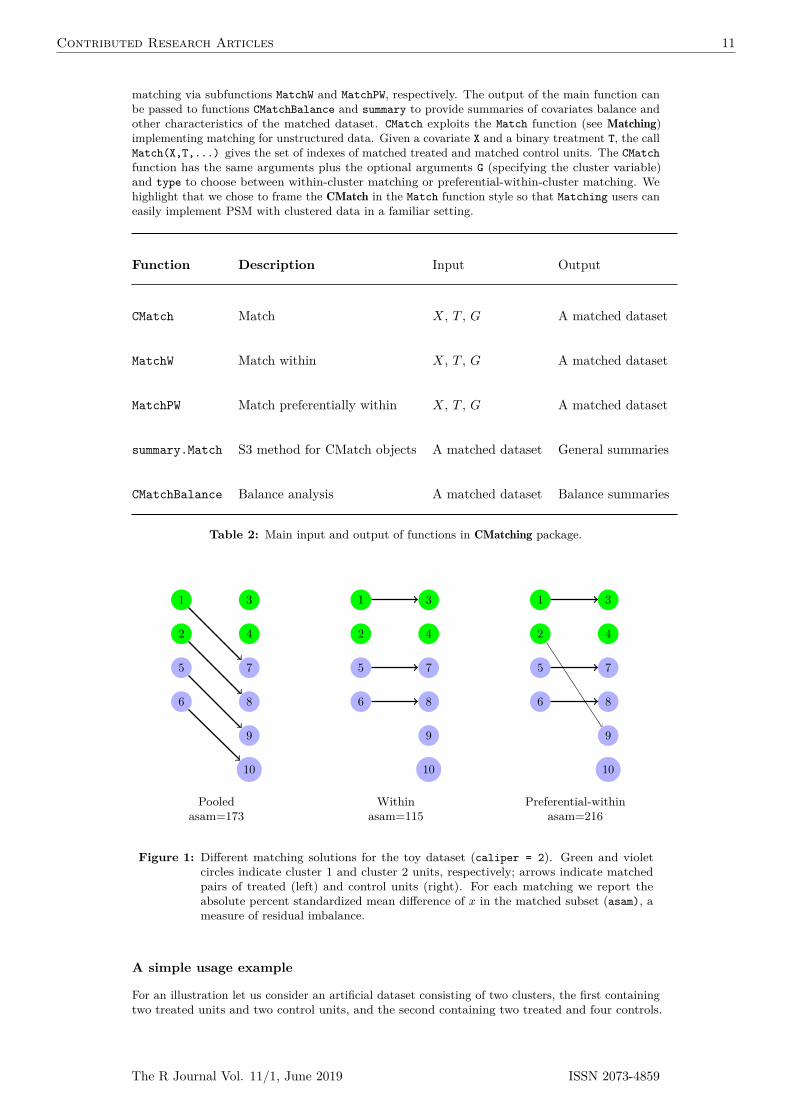
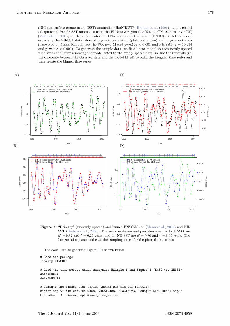
Figure 1: Different matching solutions for the toy dataset (caliper = 2). Green and violetcircles indicate cluster 1 and cluster 2 units, respectively; arrows indicate matchedpairs of treated (left) and control units (right). For each matching we report theabsolute percent standardized mean difference of x in the matched subset (asam), ameasure of residual imbalance.
A simple usage example
For an illustration let us consider an artificial dataset consisting of two clusters, the first containingtwo treated units and two control units, and the second containing two treated and four controls.
The R Journal Vol. 11/1, June 2019 ISSN 2073-4859
Contributed Research Articles 12
We use g for the cluster identifier, x for the value of the individual level confounder, and t for thebinary treatment indicator:
We also fix a caliper of 2 (in standard deviation units of X, i.e., all units at distance greater orequal than 2 ¨ sdpxq « 2 ¨ 0.312 “ 0.624 will not be matched together) and we assume that the ATTis the target parameter. Although artificial the dataset aims at representing the general situationwhere pooled matching results in matched treated and control units not distributed homogeneouslyacross clusters (see Figure 1, left).
The pooled, within and preferential-within matchings for the toy data are depicted in Figure 1.For each matching we report the asam, a measure of residual imbalance given by the absolutepercent mean difference of x across treated and controls divided by standard deviation of the treatedobservations alone. The asam is widely used as a measure of imbalance (Stuart, 2010); its value inthe unmatched data is 491. The pooled matching (left) is a complete matching, i.e., all the treatedunits could be matched. However, note that units in pairs 1-7 and 2-8 may differ in cluster levelcovariates. Matching within-cluster (center) guarantees perfect balance in cluster level covariatesbut it is incomplete because unit 2 cannot be matched within-cluster with the given caliper. This isa typical disadvantage of within-cluster matching with smaller clusters. Unit 2 is matched with 9 inthe preferential within matching (right), which again is a complete matching.
The above matching solutions can be obtained easily using CMatch as follows. For the pooledmatching it is enough to call Match (or, equivalently, CMatch without type specification) while forwithin and preferential-within matching it is enough to specify the appropriate type in the Matchcall:
# same output as before (with a warning about the absence of groups,# ties=FALSE,replace=FALSE)pm <- CMatch(type="within", Y=NULL, Tr=t, X=x, Group=NULL, caliper=2)
The output of these object is quite rich. However, a quick look at the matchings can be obtainedby directly calling the index set of matched observations:
Note that vertical alignments in the table above correspond to arrows in Figure 1. With largerdatasets and when multiple matches are allowed (i.e., when replace=TRUE) it is probably better tosummarize the output. The output objects are of class "CMatch" and a summary method is availablefor these objects. The summary shows the number of treated and the number of controls by group.Moreover, when Y is not NULL it also shows the point estimate of ATT with its model-basedestimate of the standard error:
> summary(wm)
Estimate... 0
The R Journal Vol. 11/1, June 2019 ISSN 2073-4859
Contributed Research Articles 13
SE......... NULL
Original number of observations.............. 10Original number of treated obs............... 4Original number of treated obs by group......
1 22 2
Matched number of observations............... 3Matched number of observations (unweighted). 3
Caliper (SDs).......................................... 2Number of obs dropped by 'exact' or 'caliper' ......... 1Number of obs dropped by 'exact' or 'caliper' by group
1 21 0
This summary method does not conflict with the corresponding method for class "Match" whichis still available for objects of that class. From the summary above (see also Figure 1, center) we caneasily see that matching within groups resulted in one unmatched treated unit from group two. Theexact pairing can be recovered from the full output, in particular from the object mdata containingthe list of matched and unmatched units. As we noticed in the introduction, it is essential to analyzecovariate balance to evaluate the effectiveness of matching as a balancing tool. To this end objectsof class "CMatch" can be input of the CMatchBalance function, a wrapper of MatchBalance whichoffers a large number of balance diagnostics:
> CMatchBalance( t~x , match.out=wm)
***** (V1) x *****Before Matching After Matching
mean treatment........ 1.05 1.0667mean control.......... 1.3333 1.1333std mean diff......... -490.75 -115.47(...)
From the output we see that the asam decreased from 491 to 115. One can more directly obtainthe standardized difference in means of these matchings by subcomponents:
> bwm$After[[1]]["sdiff"]$sdiff[1] -115.4701
> bpwm$After[[1]]["sdiff"]$sdiff[1] -216.5064
Whilst artificial, the previous example prompts some general considerations:
• forcing within-cluster matching may result in suboptimal matches with respect to pooledmatching. In the toy example, unit 2 is best matched with unit 8 but it is unmatched whentype=within is chosen (or it could be matched with a less similar control in the same cluster).In both cases the increased bias (due to either incomplete matching or greater imbalancein the observed x) may be at least in part compensated by lower imbalance in cluster levelvariables;
• preferential-within matching may occasionally recover all unmatched treated units in thewithin step by matching them between in step 2. However, this complete matching is generallydifferent from the complete pooled matching obtained by ignoring the clustering. In thetoy example, unit 2 is recovered in the preferential step but the final matching has a higherimbalance than the pooled one. Again, it is up to the researcher to tune the trade-off betweenbias due to incomplete matching and bias due to unobserved differences in group covariates.
In applications, when cluster level confounders are unobserved, it is not straightforward to decidewhich of the matching strategies is the best. However, combining the within and preferential-withinroutines offered by CMatching with sound subject matter knowledge, the researcher can decide howmuch importance should be given to balance within-clusters based on the hypothesized strength
The R Journal Vol. 11/1, June 2019 ISSN 2073-4859
Contributed Research Articles 14
of unobserved cluster level confounders. Note that CMatching uses the same caliper for clusters,under the assumption that the researcher is typically interested in estimating the causal effect ofthe treatment in the whole population of treated units and not by each cluster. This is the maindifference between MatchW and Matchby from the Matching package. The latter exactly matcheson a categorical variable and the caliper is recalculated in each subset and for this reason MatchWestimates generally differ from those obtained from Matchby. Another difference is that Matchbydoes not adjust standard errors for within-cluster correlation in the outcome. A third difference isthat CMatching provides some statistics (e.g., number of drops) by cluster to better appreciate howwell the matched dataset resembles the original clustered structure in terms for example of clustersize.
Demonstration of the CMatching package on NELS-88 data
The CMatching package includes several functions designed for matching with clustered data. Inthis section we illustrate the use of CMatching with a an educational example.
Schools dataset
The example is based on data coming from a nationally representative, longitudinal study of 8thgraders in 1988 in the US, called NELS-88. CMatching contains a selected subsample of the NELS-88data provided by Kraft and de Leeuw (1998) with 10 handpicked schools from the 1003 schoolsin the full dataset. The subsample, named schools, is a data frame with 260 observations on 19variables recording either school or student’s characteristics.
For the purpose of illustrating matching algorithms in CMatching, we consider estimation of thecausal effect of doing homework on mathematical proficiency. More specifically, our treatment is abinary variable taking value 1 for students that spent at least one hour doing math homework perweek and 0 otherwise. The latter is a transformation of the original variable "homework" giving twoalmost equal-sized groups. The outcome is math proficiency measured on a discrete scale rangingfrom 0 to 80. For simplicity we first attach the dataset (attach(schools)) and name the treatmentand the outcome variables as T and Y, respectively. The variable schid is the school identifier andwe rename it as Group:
> T <- ifelse(homework>1, 1, 0)> Y <- math> Group <- schid
Since the NELS-88 study was an observational study, we do not expect a simple comparison ofmath scores across treated and control students (those doing and those not doing math homework) togive an unbiased estimate of the "homework effect" because of possible student-level and school-levelconfounders. For the purpose of our example, we will consider the following student-level confounders:"ses" (a standardised continuous measure of family socio-economic status), "sex" (1 = male, 2 =female) and "white" (1 = white, 0 other race). The NELS-88 study also collected informationon school characteristics. In general, a researcher needs to include all potential confounders inthe matching procedure, irrespective of the hierarchical level. Here we considered one school-levelconfounder: "public" (1 = public schools, 0 = private) but it is plausible to assume that oneor more relevant confounders at the school-level are not available. It is clear that, to make theunconfoundedness assumption more plausible, richer data should be used. For example, students’motivation and parents’ involvement are potentially important confounders. Thus, the followingestimates should be interpreted with caution.
Before illustrating the use of CMatching, it is useful to get a better understanding of the datastructure. In the school dataset we have a fairly balanced number of treated and control units (128and 132, respectively). However, in some schools we have more treated than control students, withproportion of treated ranging from 20% to 78%:
From the table above we can notice that the total school sample size is fairly homogeneouswith the exception of one school (code = 62821) where the number of treated students (52) isconsiderably higher than the number of control students (15). These considerations are important forthe implementation of the within-cluster and preferential within-cluster matching algorithms. In fact,within-cluster matching can be difficult in groups where the proportion of treated units is high becausethere are relatively few controls that can potentially serve as a match. Preferential-within-clustermatching would be less restrictive.
This preliminary descriptive analysis is also useful to check if treated and control units are presentin each group. In fact, if a group is only composed of treated or control students then within-clustermatching cannot be implemented. Groups with only treated or controls should be dropped beforethe within-cluster matching algorithm is implemented. We now describe how Cmatching can beused to implement matching in our school-clustered dataset.
Propensity score matching
CMatching requires to estimate the propensity score before implementing the matching. Here weestimate propensity scores using a simple logistic regression with only main effects and then estimatethe predicted probability for each student:
We do not report the output of the propensity score model because in PSM the propensity scoreis only instrumental to implement the matching. Within-cluster propensity score matching can beimplemented by using the function CMatch with the option type="within":
The previous command implements matching on the estimated propensity score, eps, by usingdefault settings of Match (one-to-one matching with replacement and a caliper of 0.25 standarddeviations of the estimated propensity score). The output is an object of class "CMatch" and acustomized summary method for objects of this class gives the estimated ATT and the main featuresof the matched dataset:
> summary(psm_w)
Estimate... 5.2353SE......... 2.0677
Original number of observations.............. 260Original number of treated obs............... 128Original number of treated obs by group......
Matched number of observations............... 119Matched number of observations (unweighted). 120
Caliper (SDs).......................................... 0.25Number of obs dropped by 'exact' or 'caliper' ......... 9Number of obs dropped by 'exact' or 'caliper' by group
The summary starts reporting the original total number of students in our sample (260), thetotal number of treated students (128) and how they are distributed across the different schools.
The R Journal Vol. 11/1, June 2019 ISSN 2073-4859
Contributed Research Articles 16
It is of utmost importance to check how many treated units could be matched to avoid bias fromincomplete matching. For this reason the output indicates that 119 students in the treatmentgroup found a match ("Matched number of observations"), while the remaining 9 were dropped.Note that the unweighted number of treated observations that found a match ("Matched numberof observations (unweighted)") is different because of ties. Ties management can be controlledby option ties of the Match function: if ties=TRUE when one treated observation matches withmore than one control unit all possible pairs are included in the matched dataset and each pair isweighted equal to the inverse of the number of matchedcontrols. If instead ties=FALSE is used tiesare randomly broken. Note that the summary reports the number of treated matched and droppedunits because it is assumed by default the ATT is the target estimand. Then the output also reportshow the 9 unmatched treated students are distributed across schools. For example, we notice thatin one school (68448), 5 of the 13 treated students did not find a match. This is because for these5 students there was no control student in the same school with a propensity score falling withinthe caliper. The report also recalls the caliper, which was set to 0.25 standard deviations of theestimated propensity score in this example. The caliper can be set in standard deviation units usingthe homonymous argument caliper. It may be more useful to calculate the percentage of droppedunits instead of the absolute numbers. These percentages are not reported in the summary but theycan be easily retrieved from the CMatch output. For example, we can calculate the percentage ofunmatched treated units, both overall and by school:
# percentage of drops> psm_w$ndrops / psm_w$orig.treated.nobs
[1] 0.0703
# percentage of drops by school> psm_w$orig.dropped.nobs.by.group / table(Group)
confirming that the percentage of drops is very low in all schools. We could also similarly calculatethe percentage of drops over treated observations, which turn out to be high for school 64448.The next step before accepting a matching solution is the evaluation of the achieved balance ofconfounders across the treatment and control groups. To this end the package contains functionCMatchBalance that can be applied to an object of class "CMatch" to compare the balance beforeand after matching (the matched dataset must be specified in the match.out argument):
***** (V1) ses *****Before Matching After Matching
mean treatment........ 0.23211 0.24655mean control.......... -0.36947 0.14807std mean diff......... 61.315 10.086
***** (V2) as.factor(sex)2 *****Before Matching After Matching
mean treatment........ 0.52344 0.52941mean control.......... 0.46212 0.56303std mean diff......... 12.229 -6.706
***** (V3) white *****Before Matching After Matching
mean treatment........ 0.73438 0.7563mean control.......... 0.7197 0.71429std mean diff......... 3.3103 9.7458
***** (V4) public *****Before Matching After Matching
The R Journal Vol. 11/1, June 2019 ISSN 2073-4859
Contributed Research Articles 17
mean treatment........ 0.59375 0.57983mean control.......... 0.88636 0.57983std mean diff......... -59.346 0
(...)
The output reports the balance for each variable to allow the researcher to assess the effectivenessof matching in balancing each variable. Many balance metrics are provided but for simplicity ofexposition we focus on comparing on the standardized mean difference between the two groups ofstudents. Note that the asam can be easily obtained by averaging the standardized mean differences:
vec <-vector()for(i in 1:length()) vec[[i]] <- b_psm_w$AfterMatching[[i]]$sdiff> mean(abs(vec))[1] 6.634452
from which we can see that the initial asam of 34 (see Table 3) sharply decreased after matching.Balance improved dramatically for ses and public (results not shown). In fact, for the latter itwas possible to attain exact matching. This is guaranteed by within-cluster matching because itforces treated and control students to belong to the same school. For the same reason, within-clustermatching also guarantees a perfect balance of all other school-level variables (even unobservable)not included in the propensity score estimation. The balance improved also for the sex variablebut not for the dummy white (from 3.31% to 9.75%). In a real study, the investigator may attaina matching solution with an even better balance of the dummies for white and sex by changingthe propensity score model or one or more options in the matching algorithms. For example, asmaller caliper could be tried. Note that CMatchBalance is a wrapper of the MatchBalance function(Matching package) so it measures balance globally and not by group. This is acceptable also in ahierarchical context since we first and foremost consider the overall balance. While a group-by-groupbalance analysis may be useful it is only the average asam which matters when estimating the ATTon the whole population of treated units.
We highlighted that the within-cluster algorithm always guarantees a perfect balance in allcluster-level confounders as in the example above. However, note that it was not possible to matchsome treated observations and in part this can be due to the matching constrained to happen onlywithin clusters. The researcher can relax the constraint using preferential within-cluster matching.This algorithm can be invoked using the option type="pwithin" in the CMatch function:
A comparison of results between within and preferential within matching is given in Table 3.The preferential within-cluster matching was able to match all treated students ("Matched numberof obs" = 128), i.e., the number of unmatched treated students is 0 ("Number of drops" = 0).In this example, the 9 treated students that did not find a matched control within the caliper inthe same school found a control match in another school. Looking to the overall balance attainedby matching preferentially within, we can notice that preferential within-cluster matching showeda slightly higher asam than within-matching. In fact there is no clear "winner" between the twoalgorithms: the balance of the individual level variables ses and white improves slightly with thepreferential within-cluster matching while for sex the within-cluster matching is considerably better(not shown). Importantly, using preferential within-cluster matching the absolute standardized meandifference for the school-level variable public is 3.2% This is not a high value because most of thetreated units actually found a match within schools. However, this finding points to the fact thatpreferential within-cluster matching is not able to perfectly balance cluster level variables as thewithin-cluster approach.
Finally, having achieved a satisfactory balance with a very low number of drops we can estimatethe ATT on the matched dataset. When the argument Y is not NULL, an estimate is automaticallygiven otherwise the output of the CMatch function only gives information about the matching. Theestimated average effect of studying math for at least one hour per week on students’ math score is5.24 with a standard error of 2.07 when matching within schools (Table 3). It is worth mentioningthat the reported SE is model based and adjusts for non-independence of students within schools.From Table 3 we can see that the estimated ATT and SE for the preferential-within school approachare very similar to those obtained with the within-cluster approach. We stress that the estimatedATT should be considered carefully and only after checking the matching solution.
In conclusion, preferential within-cluster matching is expected to improve the solution of thewithin-cluster matching in terms of a reduced number of unmatched units. On the other hand,
Table 3: Matching to allow a fair comparison of math test score of students doing (treated)and not doing homework in a school clustered dataset (NELS-88 data): comparingmatching solutions obtained from CMatching.
within-cluster matching guarantees a perfect balance of school-level variables (both observed andunobserved) while preferential within does not. The researcher, choosing between the two algorithms,has to consider the trade-off between having a perfect balance of cluster level variables (within-clustermatching) or reducing the number of unmatched treated units (preferential within-cluster matching).The researcher can also implement both approaches and compare the results as a sort of sensitivityanalysis.
Multivariate covariate matching
Instead of matching on the propensity score, the researcher may match directly on the covariatesspace. This strategy can be advantageous when the number of covariates is fairly low and it isexpected to match exactly a large number of units on the original space. The syntax is very similarto the above for propensity score matching: the only difference is that the user indicates the covariatematrix instead of the propensity score in the X argument:
When X is a matrix, the covariate distance between a treated and a control unit is measured byMahalanobis metrics, i.e., essentially the multivariate Euclidean distance scaled by the standarddeviation of each covariate, a metrics which warrants an homogeneous imbalance reduction propertyfor (approximately) ellipsoidally distributed covariates (Rubin, 1980). From Table 3, columns 3-4,we can see that the balance of covariates was indeed very good. Note that the estimated ATT usingMahalanobis matching is lower than the corresponding estimate obtained with propensity scorematching. However, within-cluster matching using the Mahalanobis distance has generated a large
The R Journal Vol. 11/1, June 2019 ISSN 2073-4859
Contributed Research Articles 19
number of unmatched treated units (44). Therefore, in this case preferential within-cluster matchingcould be used to avoid an high proportion of drops.
Other strategies
Other strategies for controlling unobserved cluster covariates in PSM have been suggested by Arpinoand Mealli (2011). The basic idea is to account for the clustering in the estimation of the propensityscore by using random- or fixed-effects models. This strategy can be combined with the matchingstrategies presented before in order to ’doubly’ account for the clustering. This can be done easilywith CMatching. As an example we consider estimating the propensity score with a logit model withdummies for schools and then matching preferentially within-schools using the estimated propensityscore:
# estimate ps> mod <- glm(T ~ ses + parented + public + sex + race + urban
# match within on eps> dpsm <- CMatch(type="pwithin", Y=math, Tr=T, X=eps, Group=NULL)
In concluding this section, we also mention some other matching strategies which can beimplemented using CMatching and some programming effort. First, the utility of the algorithmsnaturally extends when there are more than two levels. In this case, it can be useful to matchpreferentially on increasingly general levels, for example by allowing individuals to be matched firstbetween regions and then between countries. Another natural extension involves data where unitshave multiple membership at the same hierarchical level. In this case it is possible to combine matchwithin (or preferential-within) across levels, for example by matching students both within schoolsand within living district (e.g. 1 out of 4 possible combinations).
Summary
In this paper we presented the package CMatching implementing matching algorithms for clustereddata. The package allows users to implement two algorithms: i) within-cluster matching andii) preferential within-cluster matching. The algorithms provide a model-based estimate of thecausal effect and its standard error adjusted for within-cluster correlation among observations. Inaddition, a tailored summary method and a balance function are provided to analyze the output. Weillustrated the case for within and preferential within-cluster matching analyzing data on studentsenrolled in different schools for which it is reasonable to assume important confounding at the schoollevel. Finally, since the analysis of clustered observational data is an active area of research, we arewilling to improve on standard error calculations for matching estimators with clustered data if newtheoretical results in the causal inference literature will become available.
Bibliography
B. Arpino and M. Cannas. Propensity score matching with clustered data. An application to theestimation of the impact of caesarean section on the Apgar score. Statistics in Medicine, 35(12):2074–2091, 2016. URL https://10.1002/sim.6880. sim.6880. [p7, 9, 10]
B. Arpino and F. Mealli. The specification of the propensity score in multilevel observational studies.Computational Statistics & Data Analysis, 55:1770–1780, 2011. URL https://dx.doi.org/10.1016/j.csda.2010.11.008. [p7, 19]
G. Cafri, W. Wang, P. H. Chan, and P. C. Austin. A review and empirical comparison of causalinference methods for clustered observational data with application to the evaluation of theeffectiveness of medical devices. Statistical Methods in Medical Research, 0(0):0962280218799540,2018. URL https://10.1177/0962280218799540. [p7, 10]
A. C. Cameron, J. B. Gelbach, and D. L. Miller. Robust inference with multiway clustering. Journal ofBusiness & Economic Statistics, 29(2):238–249, 2011. URL https://10.1198/jbes.2010.07136.[p9]
A. Diamond and J. S. Sekhon. Genetic matching for estimating causal effects: A general multivariatematching method for achieving balance in observational studies. Review of Economics andStatistics, 95(3):932–945, 2013. URL https://doi.org/10.1162/REST_a_00318. [p8]
B. B. Hansen and S. O. Klopfer. Optimal full matching and related designs via network flows.Journal of Computational and Graphical Statistics, 15(3):609–627, 2006. URL https://10.1198/106186006X137047. [p8]
D. E. Ho, K. Imai, G. King, and E. A. Stuart. Matching as nonparametric preprocessing for reducingmodel dependence in parametric causal inference. Political Analysis, 15(3):199–236, 2007. URLhttps://10.1093/pan/mpl013. [p9]
P. W. Holland. Statistics and causal inference. Journal of the American Statistical Association, 81(396):945–960, 1986. [p9]
S. M. Iacus, G. King, and G. Porro. Multivariate matching methods that are monotonic imbalancebounding. Journal of the American Statistical Association, 106(493):345–361, 2011. URL https://doi.org/10.1198/jasa.2011.tm09599. [p8]
G. W. Imbens and D. B. Rubin. Causal Inference for Statistics, Social and Biomedical Sciences.John Wiley & Sons, 2016. [p7]
I. Kraft and J. de Leeuw. Introducing Multilevel Modeling. London, Sage, 1998. [p14]
F. Li, A. M. Zaslavsky, and M. B. Landrum. Propensity score weighting with multilevel data. Statisticsin Medicine, 32(19):3373–3387, 2013. ISSN 1097-0258. URL https://10.1002/sim.5786. [p7, 9]
J. H. Rickles and M. Seltzer. A two-stage propensity score matching strategy for treatment effectestimation in a multisite observational study. Journal of Educational and Behavioral Statistics, 39(6):612–636, 2014. URL https://10.3102/1076998614559748. [p7, 10]
P. Rosenbaum and D. Rubin. The central role of the propensity score in observational studies forcausal effects. Biometrika, 70:41–55, 1983. URL https://10.2307/2335942. [p7]
P. Rosenbaum and D. Rubin. Constructing a control group using multivariate matched samplingmethods that incorporate the propensity score. The American Statistician, 39:33–38, 1985. URLhttps://doi.org/10.1080/00031305.1985.10479383. [p9]
D. B. Rubin. Bias reduction using mahalanobis-metric matching. Biometrics, 36(2):293–298, 1980.URL https://10.2307/2529981. [p18]
F. Savje, J. Sekhon, and M. Higgins. Quickmatch: Quick Generalized Full Matching, 2018. URLhttps://CRAN.R-project.org/package=quickmatch. R package version 0.2.1. [p8]
J. S. Sekhon. Multivariate and propensity score matching software with automated balance opti-mization: The Matching package for R. Journal of Statistical Software, 42(7):1–52, 2011. URLhttps://dx.doi.org/10.18637/jss.v042.i07. [p8]
E. A. Stuart. Matching methods for causal inference: A review and a look forward. Statist. Sci., 25(1):1–21, 2010. URL https://10.1214/09-STS313. [p7, 12]
J. R. Zubizarreta, C. Kilcioglu, and J. P. Vielma. Designmatch: Matched Samples That Are Balancedand Representative by Design, 2018. URL https://CRAN.R-project.org/package=designmatch.R package version 0.3.1. [p8]
R. J. Zubizarreta and L. Keele. Optimal multilevel matching in clustered observational studies: Acase study of the effectiveness of private schools under a large-scale voucher system. Journalof the American Statistical Association, 112:0, 2017. URL https://doi.org/10.1080/01621459.2016.1240683. [p7]
Time-Series Clustering in R Using thedtwclust Packageby Alexis Sardá-Espinosa
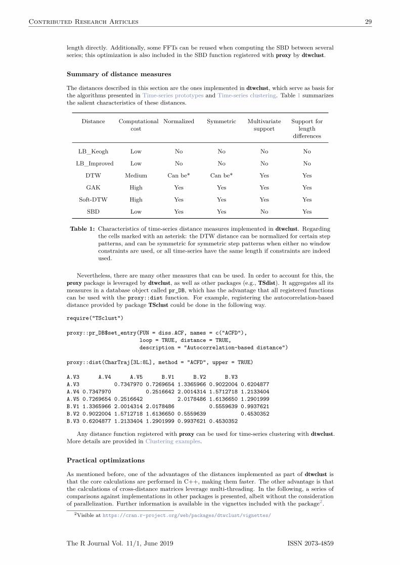
Abstract Most clustering strategies have not changed considerably since their initial definition.The common improvements are either related to the distance measure used to assess dissimilarity, orthe function used to calculate prototypes. Time-series clustering is no exception, with the DynamicTime Warping distance being particularly popular in that context. This distance is computationallyexpensive, so many related optimizations have been developed over the years. Since no singleclustering algorithm can be said to perform best on all datasets, different strategies must be testedand compared, so a common infrastructure can be advantageous. In this manuscript, a generaloverview of shape-based time-series clustering is given, including many specifics related to DynamicTime Warping and associated techniques. At the same time, a description of the dtwclust packagefor the R statistical software is provided, showcasing how it can be used to evaluate many differenttime-series clustering procedures.
Introduction
Cluster analysis is a task that concerns itself with the creation of groups of objects, where eachgroup is called a cluster. Ideally, all members of the same cluster are similar to each other, but areas dissimilar as possible from objects in a different cluster. There is no single definition of a cluster,and the characteristics of the objects to be clustered vary. Thus, there are several algorithms toperform clustering. Each one defines specific ways of defining what a cluster is, how to measuresimilarities, how to find groups efficiently, etc. Additionally, each application might have differentgoals, so a certain clustering algorithm may be preferred depending on the type of clusters sought(Kaufman and Rousseeuw, 1990).
Clustering algorithms can be organized differently depending on how they handle the data andhow the groups are created. When it comes to static data, i.e., if the values do not change withtime, clustering methods can be divided into five major categories: partitioning (or partitional),hierarchical, density-based, grid-based, and model-based methods (Liao, 2005; Rani and Sikka,2012). They may be used as the main algorithm, as an intermediate step, or as a preprocessing step(Aghabozorgi et al., 2015).
Time-series is a common type of dynamic data that naturally arises in many different scenarios,such as stock data, medical data, and machine monitoring, just to name a few (Aghabozorgi et al.,2015; Aggarwal and Reddy, 2013). They pose some challenging issues due to the large size and highdimensionality commonly associated with time-series (Aghabozorgi et al., 2015). In this context,dimensionality of a series is related to time, and it can be understood as the length of the series.Additionally, a single time-series object may be constituted by several values that change on thesame time scale, in which case they are identified as multivariate time-series.
There are many techniques to modify time-series in order to reduce dimensionality, and theymostly deal with the way time-series are represented. Changing representation can be an importantstep, not only in time-series clustering, and it constitutes a wide research area on its own (cf. Table2 in Aghabozorgi et al. (2015)). While choice of representation can directly affect clustering, it canbe considered as a different step, and as such it will not be discussed further here.
Time-series clustering is a type of clustering algorithm made to handle dynamic data. The mostimportant elements to consider are the (dis)similarity or distance measure, the prototype extractionfunction (if applicable), the clustering algorithm itself, and cluster evaluation (Aghabozorgi et al.,2015). In many cases, algorithms developed for time-series clustering take static clustering algorithmsand either modify the similarity definition, or the prototype extraction function to an appropriate one,or apply a transformation to the series so that static features are obtained (Liao, 2005). Therefore,the underlying basis for the different clustering procedures remains approximately the same acrossclustering methods. The most common approaches are hierarchical and partitional clustering (cf.Table 4 in Aghabozorgi et al. (2015)), the latter of which includes fuzzy clustering.
Aghabozorgi et al. (2015) classify time-series clustering algorithms based on the way they treatthe data and how the underlying grouping is performed. One classification depends on whether thewhole series, a subsequence, or individual time points are to be clustered. On the other hand, theclustering itself may be shape-based, feature-based, or model-based. Aggarwal and Reddy (2013)make an additional distinction between online and offline approaches, where the former usually dealswith grouping incoming data streams on-the-go, while the latter deals with data that no longer
change.In the context of shape-based time-series clustering, it is common to utilize the Dynamic Time
Warping (DTW) distance as dissimilarity measure (Aghabozorgi et al., 2015). The calculation of theDTW distance involves a dynamic programming algorithm that tries to find the optimum warpingpath between two series under certain constraints. However, the DTW algorithm is computationallyexpensive, both in time and memory utilization. Over the years, several variations and optimizationshave been developed in an attempt to accelerate or optimize the calculation. Some of the mostcommon techniques will be discussed in more detail in Dynamic time warping distance.
The choice of time-series representation, preprocessing, and clustering algorithm has a big impacton performance with respect to cluster quality and execution time. Similarly, different programminglanguages have different run-time characteristics and user interfaces, and even though many authorsmake their algorithms publicly available, combining them is far from trivial. As such, it is desirableto have a common platform on which clustering algorithms can be tested and compared against eachother. The dtwclust package, developed for the R statistical software, and part of its TimeSeriesview, provides such functionality, and includes implementations of recently developed time-seriesclustering algorithms and optimizations. It serves as a bridge between classical clustering algorithmsand time-series data, additionally providing visualization and evaluation routines that can handletime-series. All of the included algorithms are custom implementations, except for the hierarchicalclustering routines. A great amount of effort went into implementing them as efficiently as possible,and the functions were designed with flexibility and extensibility in mind.
Most of the included algorithms and optimizations are tailored to the DTW distance, hence thepackage’s name. However, the main clustering function is flexible so that one can test many differentclustering approaches, using either the time-series directly, or by applying suitable transformationsand then clustering in the resulting space. We will describe the new algorithms that are available indtwclust, mentioning the most important characteristics of each, and showing how the package canbe used to evaluate them, as well as how other packages complement it. Additionally, the variationsrelated to DTW and other common distances will be explored.
There are many available R packages for data clustering. The flexclust package (Leisch, 2006)implements many partitional procedures, while the cluster package (Maechler et al., 2019) focusesmore on hierarchical procedures and their evaluation; neither of them, however, is specificallytargeted at time-series data. Packages like TSdist (Mori et al., 2016) and TSclust (Montero andVilar, 2014) focus solely on dissimilarity measures for time-series, the latter of which includes a singlealgorithm for clustering based on p values. Another example is the pdc package (Brandmaier, 2015),which implements a specific clustering algorithm, namely one based on permutation distributions.The dtw package (Giorgino, 2009) implements extensive functionality with respect to DTW, butdoes not include the lower bound techniques that can be very useful in time-series clustering. Newclustering algorithms like k-Shape (Paparrizos and Gravano, 2015) and TADPole (Begum et al.,2015) are available to the public upon request, but were implemented in MATLAB, making theircombination with other R packages cumbersome. Hence, the dtwclust package is intended to providea consistent and user-friendly way of interacting with classic and new clustering algorithms, takinginto consideration the nuances of time-series data.
The rest of this manuscript presents the different logical units required for a time-series clusteringworkflow, and specifies how they are implemented in dtwclust. These build on top of each other andare not entirely independent, so their coherent combination is critical. The information relevant tothe distance measures will be presented in Distance measures. Supported algorithms for prototypeextraction will be discussed in Time-series prototypes. The main clustering algorithms will beintroduced in Time-series clustering. Information regarding cluster evaluation will be providedin Cluster evaluation. The provided tools for a complete time-series clustering workflow will bedescribed in Comparing clustering algorithms with dtwclust, and the final remarks will be givenin Conclusion. Note that code examples are intentionally brief, and do not necessarily represent athorough procedure to choose or evaluate a clustering algorithm. The data used in all examples isincluded in the package (saved in a list called CharTraj), and is a subset of the character trajectoriesdataset found in Lichman (2013): they are pen tip trajectories recorded for individual characters,and the subset contains 5 examples of the x velocity for each considered character.
Distance measures
Distance measures provide quantification for the dissimilarity between two time-series. Calculatingdistances, as well as cross-distance matrices, between time-series objects is one of the cornerstonesof any time-series clustering algorithm. The proxy package (Meyer and Buchta, 2019) providesan extensible framework for these calculations, and is used extensively by dtwclust; Summary ofdistance measures will elaborate in this regard.
The l1 and l2 vector norms, also known as Manhattan and Euclidean distances respectively, arethe most commonly used distance measures, and are arguably the only competitive lp norms whenmeasuring dissimilarity (Aggarwal et al., 2001; Lemire, 2009). They can be efficiently computed,but are only defined for series of equal length and are sensitive to noise, scale, and time shifts. Thus,many other distance measures tailored to time-series have been developed in order to overcome theselimitations, as well as other challenges associated with the structure of time-series, such as multiplevariables, serial correlation, etc.
In the following sections a description of the distance functions included in dtwclust will beprovided; these are associated with shape-based time-series clustering, and either support DTW orprovide an alternative to it. The included distances are a basis for some of the prototyping functionsdescribed in Time-series prototypes, as well as the clustering routines from Time-series clustering, butthere are many other distance measures that can be used for time-series clustering and classification(Montero and Vilar, 2014; Mori et al., 2016). It is worth noting that, even though some of thesedistances are also available in other R packages, e.g., DTW in dtw or Keogh’s DTW lower boundin TSdist (see Dynamic time warping distance), the implementations in dtwclust are optimizedfor speed, since all of them are implemented in C++ and have custom loops for computation ofcross-distance matrices, including multi-threading support; refer to Practical optimizations for moreinformation.
To facilitate notation, we define a time-series as a vector (or set of vectors in case of multivariateseries) x. Each vector must have the same length for a given time-series. In general, xvi representsthe i-th element of the v-th variable of the (possibly multivariate) time-series x. We will assumethat all elements are equally spaced in time in order to avoid the time index explicitly.
Dynamic time warping distance
DTW is a dynamic programming algorithm that compares two series and tries to find the optimumwarping path between them under certain constraints, such as monotonicity (Berndt and Clifford,1994). It started being used by the data mining community to overcome some of the limitationsassociated with the Euclidean distance (Ratanamahatana and Keogh, 2004).
The easiest way to get an intuition of what DTW does is graphically. Figure 1 shows thealignment between two sample time-series x and y. In this instance, the initial and final points ofthe series must match, but other points may be warped in time in order to find better matches.
Time
Ser
ies
0 50 100 150
−0.
40.
20.
6
−1
−0.
50
0.5
1
Figure 1: Sample alignment performed by the DTW algorithm between two series. The dashedblue lines exemplify how some points are mapped to each other, which shows how theycan be warped in time. Note that the vertical position of each series was artificiallyaltered for visualization.
DTW is computationally expensive. If x has length n and y has length m, the DTW distancebetween them can be computed inOpnmq time, which is quadratic ifm and n are similar. Additionally,DTW is prone to implementation bias since its calculations are not easily vectorized and tend to bevery slow in non-compiled programming languages. A custom implementation of the DTW algorithmis included with dtwclust in the dtw_basic function, which has only basic functionality but stillsupports the most common options, and it is faster (see Practical optimizations).
The DTW distance can potentially deal with series of different length directly. This is notnecessarily an advantage, as it has been shown before that performing linear reinterpolation to
The R Journal Vol. 11/1, June 2019 ISSN 2073-4859
Contributed Research Articles 25
obtain equal length may be appropriate if m and n do not vary significantly (Ratanamahatana andKeogh, 2004). For a more detailed explanation of the DTW algorithm see, e.g., Giorgino (2009).However, there are some aspects that are worth discussing here.
The first step in DTW involves creating a local cost matrix (LCM or lcm), which has nˆmdimensions. Such a matrix must be created for every pair of distances compared, meaning thatmemory requirements may grow quickly as the dataset size grows. Considering x and y as the inputseries, for each element pi, jq of the LCM, the lp norm between xi and yj must be computed. This isdefined in Equation 1, explicitly denoting that multivariate series are supported as long as they havethe same number of variables (note that for univariate series, the LCM will be identical regardlessof the used norm). Thus, it makes sense to speak of a DTWp distance, where p corresponds to thelp norm that was used to construct the LCM.
lcmpi, jq “˜
ÿ
v
|xvi ´ yvj |p
¸1p
(1)
In the seconds step, the DTW algorithm finds the path that minimizes the alignment between xand y by iteratively stepping through the LCM, starting at lcmp1, 1q and finishing at lcmpn,mq,and aggregating the cost. At each step, the algorithm finds the direction in which the cost increasesthe least under the chosen constraints.
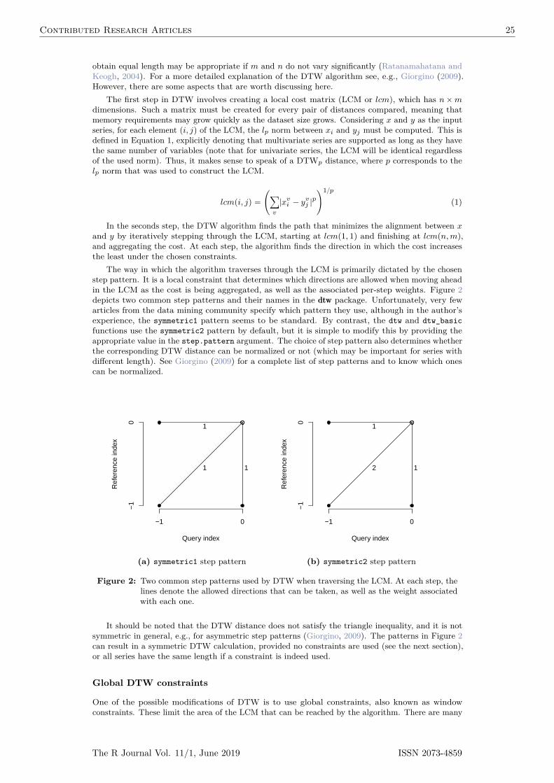
The way in which the algorithm traverses through the LCM is primarily dictated by the chosenstep pattern. It is a local constraint that determines which directions are allowed when moving aheadin the LCM as the cost is being aggregated, as well as the associated per-step weights. Figure 2depicts two common step patterns and their names in the dtw package. Unfortunately, very fewarticles from the data mining community specify which pattern they use, although in the author’sexperience, the symmetric1 pattern seems to be standard. By contrast, the dtw and dtw_basicfunctions use the symmetric2 pattern by default, but it is simple to modify this by providing theappropriate value in the step.pattern argument. The choice of step pattern also determines whetherthe corresponding DTW distance can be normalized or not (which may be important for series withdifferent length). See Giorgino (2009) for a complete list of step patterns and to know which onescan be normalized.
Query index
Ref
eren
ce in
dex
1 1
1
−1 0
−1
0
(a) symmetric1 step pattern
Query index
Ref
eren
ce in
dex
2 1
1
−1 0
−1
0
(b) symmetric2 step pattern
Figure 2: Two common step patterns used by DTW when traversing the LCM. At each step, thelines denote the allowed directions that can be taken, as well as the weight associatedwith each one.
It should be noted that the DTW distance does not satisfy the triangle inequality, and it is notsymmetric in general, e.g., for asymmetric step patterns (Giorgino, 2009). The patterns in Figure 2can result in a symmetric DTW calculation, provided no constraints are used (see the next section),or all series have the same length if a constraint is indeed used.
Global DTW constraints
One of the possible modifications of DTW is to use global constraints, also known as windowconstraints. These limit the area of the LCM that can be reached by the algorithm. There are many
The R Journal Vol. 11/1, June 2019 ISSN 2073-4859
Contributed Research Articles 26
types of windows (see, e.g., Giorgino (2009)), but one of the most common ones is the Sakoe-Chibawindow (Sakoe and Chiba, 1978), with which an allowed region is created along the diagonal of theLCM (see Figure 3). These constraints can marginally speed up the DTW calculation, but they aremainly used to avoid pathological warping. It is common to use a window whose size is 10% of theseries’ length, although sometimes smaller windows produce even better results (Ratanamahatanaand Keogh, 2004).
2 4 6 8 10
24
68
10
Query: samples 1..10
Ref
eren
ce: s
ampl
es 1
..10
Figure 3: Visual representation of the Sakoe-Chiba constraint for DTW. The red elements willnot be considered by the algorithm when traversing the LCM.
Strictly speaking, if the series being compared have different lengths, a constrained path may notexist, since the Sakoe-Chiba band may prevent the end point of the LCM to be reached (Giorgino,2009). In these cases a slanted band window may be preferred, since it stays along the diagonal forseries of different length and is equivalent to the Sakoe-Chiba window for series of equal length. If awindow constraint is used with dtwclust, a slanted band is employed.
It is not possible to know a priori what window size, if any, will be best for a specific application,although it is usually agreed that no constraint is a poor choice. For this reason, it is better toperform tests with the data one wants to work with, perhaps taking a subset to avoid excessiverunning times.
It should be noted that, when reported, window sizes are always integers greater than zero. Ifwe denote this number with w, and for the specific case of the slanted band window, the valid regionof the LCM will be constituted by all valid points in the range rpi, j ´wq, pi, j `wqs for all pi, jqalong the LCM diagonal. Thus, at each step, at most 2w` 1 elements may fall within the windowfor a given window size w. This is the convention followed by dtwclust.
Lower bounds for DTW
Due to the fact that DTW itself is expensive to compute, lower bounds (LBs) for the DTW distancehave been developed. These lower bounds guarantee being less than or equal to the correspondingDTW distance. They have been exploited when indexing time-series databases, classification oftime-series, clustering, etc. (Keogh and Ratanamahatana, 2005; Begum et al., 2015). Out of theexisting DTW LBs, the two most effective are termed LB_Keogh (Keogh and Ratanamahatana,2005) and LB_Improved (Lemire, 2009). The reader is referred to the respective articles for detaileddefinitions and proofs of the LBs, however some important considerations will be further discussedhere.
Each LB can be computed with a specific lp norm. Therefore, it follows that the lp norms usedfor DTW and LB calculations must match, such that LBp ď DTWp. Moreover, LB_Keoghp ďLB_Improvedp ď DTWp, meaning that LB_Improved can provide a tighter LB. It must be notedthat the LBs are only defined for series of equal length and are not symmetric regardless of the lpnorm used to compute them. Also note that the choice of step pattern affects the value of the DTWdistance, changing the tightness of a given LB.
One crucial step when calculating the LBs is the computation of the so-called envelopes. Theseenvelopes require a window constraint, and are thus dependent on both the type and size of thewindow. Based on these, a running minimum and maximum are computed, and a lower and upperenvelope are generated respectively. Figure 4 depicts a sample time-series with its correspondingenvelopes for a Sakoe-Chiba window of size 15.
In order for the LBs to be worth it, they must be computed in significantly less time than it takes
The R Journal Vol. 11/1, June 2019 ISSN 2073-4859
Contributed Research Articles 27
0 50 100 150
−0.
50.
00.
51.
0
Time
Ser
ies
Figure 4: Visual representation of a time-series (shown as a solid black line) and its correspondingenvelopes based on a Sakoe-Chiba window of size 15. The green dashed line representsthe upper envelope, while the red dashed line represents the lower envelope.
to calculate the DTW distance. Lemire (2009) developed a streaming algorithm to calculate theenvelopes using no more than 3n comparisons when using a Sakoe-Chiba window. This algorithmhas been ported to dtwclust using the C++ programming language, ensuring an efficient calculation,and it is exposed in the compute_envelope function.
LB_Keogh requires the calculation of one set of envelopes for every pair of series compared,whereas LB_Improved must calculate two sets of envelopes for every pair of series. If the LBs must becalculated between several time-series, some envelopes can be reused when a given series is comparedagainst many others. This optimization is included in the LB functions registered with proxy bydtwclust.
Global alignment kernel distance
Cuturi (2011) proposed an algorithm to assess similarity between time series by using kernels. Hebegan by formalizing an alignment between two series x and y as π, and defined the set of all possiblealignments as Apn,mq, which is constrained by the lengths of x and y. It is shown that the DTWdistance can be understood as the cost associated with the minimum alignment.
A Global Alignment (GA) kernel that considers the cost of all possible alignments by computingtheir exponentiated soft-minimum is defined, and it is argued that it quantifies similarities in a morecoherent way. However, the GA kernel has associated limitations, namely diagonal dominance anda complexity Opnmq. With respect to the former, Cuturi (2011) states that diagonal dominanceshould not be an issue as long as one of the series being compared is not longer than twice thelength of the other.
In order to reduce the GA kernel’s complexity, Cuturi (2011) proposed using the triangularlocal kernel for integers shown in Equation 2, where T represents the kernel’s order. By combiningit with the kernel κ in Equation 3 (which is based on the Gaussian kernel κσ), the TriangularGlobal Alignment Kernel (TGAK) in Equation 4 is obtained. Such a kernel can be computed inOpT minpn,mqq, and is parameterized by the triangular constraint T and the Gaussian’s kernelwidth σ.
ωpi, jq “ˆ
1´ |i´ j|T
˙
`
(2)
κpx, yq “ e´φσpx,yq (3a)
φσpx, yq “ 12σ2 ‖x´ y‖2
` logˆ
2´ e´‖x´y‖2
2σ2
˙
(3b)
TGAKpx, y,σ,T q “ τ´1ˆ
ωb12κ
˙
pi,x; j, yq “ ωpi, jqκpx, yq2´ ωpi, jqκpx, yq (4)
The triangular constraint is similar to the window constraints that can be used in the DTWalgorithm. When T “ 0 or T Ñ8, the TGAK converges to the original GA kernel. When T “ 1,
The R Journal Vol. 11/1, June 2019 ISSN 2073-4859
Contributed Research Articles 28
the TGAK becomes a slightly modified Gaussian kernel that can only compare series of equal length.If T ą 1, then only the alignments that fulfil ´T ă π1piq ´ π2piq ă T are considered.
Cuturi (2011) also proposed a strategy to estimate the value of σ based on the time-seriesthemselves and their lengths, namely c ¨medp‖x´ y‖q ¨
a
medp|x|q, where medp¨q is the empiricalmedian, c is some constant, and x and y are subsampled vectors from the dataset. This, however,introduces some randomness into the algorithm when the value of σ is not provided, so it might bebetter to estimate it once and re-use it in subsequent function evaluations. In dtwclust, the value ofc is set to 1.
The similarity returned by the TGAK can be normalized with Equation 5 so that its values liein the range r0, 1s. Hence, a distance measure for time-series can be obtained by subtracting thenormalized value from 1. The algorithm supports multivariate series and series of different length(with some limitations). The resulting distance is symmetric and satisfies the triangle inequality,although it is more expensive to compute in comparison to DTW.
A C implementation of the TGAK algorithm is available at its author’s website1. An R wrapperhas been implemented in dtwclust in the GAK function, performing the aforementioned normalizationand subtraction in order to obtain a distance measure that can be used in clustering procedures.
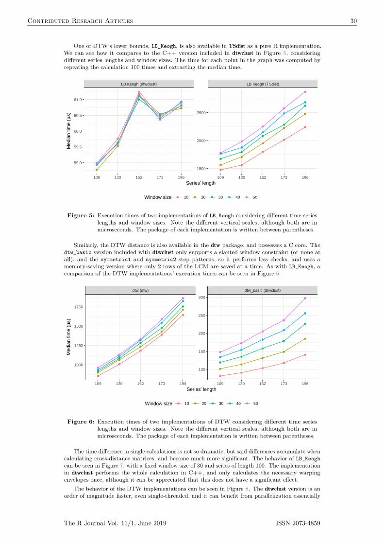
Soft-DTW
Following with the idea of the TGAK, i.e., of regularizing DTW by smoothing it, Cuturi and Blondel(2017) proposed a unified algorithm using a parameterized soft-minimum as shown in Equation 6(where ∆px, yq represents the LCM), and called the resulting discrepancy a soft-DTW, discussingits differentiability. Thanks to this property, a gradient function can be obtained, and Cuturi andBlondel (2017) developed a more efficient way to compute it. This can be then used to calculatecentroids with numerical optimization as discussed in Soft-DTW centroid.
dtwγpx, yq “ minγtxA, ∆px, yqy,A P Apn,mqu (6a)
minγta1, . . . , anu “#
miniďnai, γ “ 0´γ log
řni“1 e
´aiγ , γ ą 0(6b)
However, as a stand-alone distance measure, the soft-DTW distance has some disadvantages:the distance can be negative, the distance between x and itself is not necessarily zero, it does notfulfill the triangle inequality, and also has quadratic complexity with respect to the series’ lengths.On the other hand, it is a symmetric distance, it supports multivariate series as well as differentlengths, and it can provide differently smoothed results by means of a user-defined γ.
Shape-based distance
The shape-based distance (SBD) was proposed as part of the k-Shape clustering algorithm (Paparrizosand Gravano, 2015); this algorithm will be further discussed in Shape extraction and k-Shapeclustering. SBD is presented as a faster alternative to DTW. It is based on the cross-correlationwith coefficient normalization (NCCc) sequence between two series, and is thus sensitive to scale,which is why Paparrizos and Gravano (2015) recommend z-normalization. The NCCc sequence isobtained by convolving the two series, so different alignments can be considered, but no point-wisewarpings are made. The distance can be calculated with the formula shown in Equation 7, where‖¨‖2 is the l2 norm of the series. Its range lies between 0 and 2, with 0 indicating perfect similarity.
SBDpx, yq “ 1´ max pNCCcpx, yqq‖x‖2 ‖y‖2
(7)
This distance can be efficiently computed by utilizing the Fast Fourier Transform (FFT) toobtain the NCCc sequence, although that might make it sensitive to numerical precision, especially in32-bit architectures. It can be very fast, it is symmetric, it was very competitive in the experimentsperformed in Paparrizos and Gravano (2015) (although the run-time comparison was slightly biaseddue to the slow MATLAB implementation of DTW), and it supports (univariate) series of different
1http://marcocuturi.net/GA.html, accessed on 2016-10-29
length directly. Additionally, some FFTs can be reused when computing the SBD between severalseries; this optimization is also included in the SBD function registered with proxy by dtwclust.
Summary of distance measures
The distances described in this section are the ones implemented in dtwclust, which serve as basis forthe algorithms presented in Time-series prototypes and Time-series clustering. Table 1 summarizesthe salient characteristics of these distances.
Distance Computationalcost
Normalized Symmetric Multivariatesupport
Support forlength
differences
LB_Keogh Low No No No No
LB_Improved Low No No No No
DTW Medium Can be* Can be* Yes Yes
GAK High Yes Yes Yes Yes
Soft-DTW High Yes Yes Yes Yes
SBD Low Yes Yes No Yes
Table 1: Characteristics of time-series distance measures implemented in dtwclust. Regardingthe cells marked with an asterisk: the DTW distance can be normalized for certain steppatterns, and can be symmetric for symmetric step patterns when either no windowconstraints are used, or all time-series have the same length if constraints are indeedused.
Nevertheless, there are many other measures that can be used. In order to account for this, theproxy package is leveraged by dtwclust, as well as other packages (e.g., TSdist). It aggregates all itsmeasures in a database object called pr_DB, which has the advantage that all registered functionscan be used with the proxy::dist function. For example, registering the autocorrelation-baseddistance provided by package TSclust could be done in the following way.
Any distance function registered with proxy can be used for time-series clustering with dtwclust.More details are provided in Clustering examples.
Practical optimizations
As mentioned before, one of the advantages of the distances implemented as part of dtwclust isthat the core calculations are performed in C++, making them faster. The other advantage is thatthe calculations of cross-distance matrices leverage multi-threading. In the following, a series ofcomparisons against implementations in other packages is presented, albeit without the considerationof parallelization. Further information is available in the vignettes included with the package2.
2Visible at https://cran.r-project.org/web/packages/dtwclust/vignettes/
One of DTW’s lower bounds, LB_Keogh, is also available in TSdist as a pure R implementation.We can see how it compares to the C++ version included in dtwclust in Figure 5, consideringdifferent series lengths and window sizes. The time for each point in the graph was computed byrepeating the calculation 100 times and extracting the median time.
LB Keogh (dtwclust) LB Keogh (TSdist)
109 130 152 173 196 109 130 152 173 196
1500
2000
2500
59.0
59.5
60.0
60.5
61.0
Series' length
Med
ian
time
(µs)
Window size 10 20 30 40 50
Figure 5: Execution times of two implementations of LB_Keogh considering different time serieslengths and window sizes. Note the different vertical scales, although both are inmicroseconds. The package of each implementation is written between parentheses.
Similarly, the DTW distance is also available in the dtw package, and possesses a C core. Thedtw_basic version included with dtwclust only supports a slanted window constraint (or none atall), and the symmetric1 and symmetric2 step patterns, so it performs less checks, and uses amemory-saving version where only 2 rows of the LCM are saved at a time. As with LB_Keogh, acomparison of the DTW implementations’ execution times can be seen in Figure 6.
dtw (dtw) dtw_basic (dtwclust)
109 130 152 173 196 109 130 152 173 196
100
150
200
250
300
1000
1250
1500
1750
Series' length
Med
ian
time
(µs)
Window size 10 20 30 40 50
Figure 6: Execution times of two implementations of DTW considering different time serieslengths and window sizes. Note the different vertical scales, although both are inmicroseconds. The package of each implementation is written between parentheses.
The time difference in single calculations is not so dramatic, but said differences accumulate whencalculating cross-distance matrices, and become much more significant. The behavior of LB_Keoghcan be seen in Figure 7, with a fixed window size of 30 and series of length 100. The implementationin dtwclust performs the whole calculation in C++, and only calculates the necessary warpingenvelopes once, although it can be appreciated that this does not have a significant effect.
The behavior of the DTW implementations can be seen in Figure 8. The dtwclust version is anorder of magnitude faster, even single-threaded, and it can benefit from parallelization essentially
Figure 7: Execution times of the two implementations of LB_Keogh when calculating cross-distance matrices. The points on the left of the dashed line represent square matrices,whereas the ones on the right only have one dimension of the cross-distance matrixincreased (the one that results in more envelope calculations). Note the differentvertical scales, although both are in milliseconds. The package of each implementationis written between parentheses.
proportionally to the number of threads available.
Figure 8: Execution times of the two implementations of DTW when calculating cross-distancematrices. Note the different vertical scales, although both are in seconds. The packageof each implementation is written between parentheses.
Time-series prototypes
A very important step of time-series clustering is the calculation of so-called time-series prototypes.It is expected that all series within a cluster are similar to each other, and one may be interested intrying to define a time-series that effectively summarizes the most important characteristics of allseries in a given cluster. This series is sometimes referred to as an average series, and prototyping isalso sometimes called time-series averaging, but we will prefer the term “prototyping”, althoughcalling them time-series centroids is also common.
Computing prototypes is commonly done as a sub-routine of a larger task. In the context
The R Journal Vol. 11/1, June 2019 ISSN 2073-4859
Contributed Research Articles 32
of clustering (see Time-series clustering), partitional procedures rely heavily on the prototypingfunction, since the resulting prototypes are used as cluster centroids. Prototyping could even bea pre-processing step, whereby different samples from the same source can be summarized beforeclustering (e.g., for the character trajectories dataset, all trajectories from the same character canbe summarized and then groups of similar characters could be sought), thus reducing the amount ofdata and execution time. Another example is time-series classification based on nearest-neighbors,which can be optimized by considering only group-prototypes as neighbors instead of the union ofall groups. Nevertheless, it is important to note that the distance used in the overall task should becongruent with the chosen centroid, e.g., using the DTW distance for DTW-based prototypes.
The choice of prototyping function is closely related to the chosen distance measure and, in asimilar fashion, it is not simple to know which kind of prototype will be better a priori. There areseveral strategies available for time-series prototyping, although due to their high dimensionality, whatexactly constitutes an average time-series is debatable, and some notions could worsen performancesignificantly. The following sections will briefly describe some of the common approaches whendealing with time-series.
Partition around medoids
One approach is to use partition around medoids (PAM). A medoid is simply a representative objectfrom a cluster, in this case also a time-series, whose average distance to all other objects in thesame cluster is minimal. Since the medoid object is always an element of the original data, PAM issometimes preferred over mean or median so that the time-series structure is not altered.
A possible advantage of PAM is that, since the data does not change, it is possible to precomputethe whole distance matrix once and re-use it on each iteration, and even across different number ofclusters and random repetitions. However, this is not suitable for large datasets since the wholedistance matrix has to be allocated at once.
In the implementation included in the package, the distances between all member series arecomputed, and the series with minimum sum of distances is chosen as the prototype.
DTW barycenter averaging
The DTW distance is used very often when working with time-series, and thus a prototyping functionbased on DTW has also been developed in Petitjean et al. (2011). The procedure is called DTWbarycenter averaging (DBA), and is an iterative, global method. The latter means that the order inwhich the series enter the prototyping function does not affect the outcome.
DBA requires a series to be used as reference (centroid), and it usually begins by randomlyselecting one of the series in the data. On each iteration, the DTW alignment between each series inthe cluster C and the centroid is computed. Because of the warping performed in DTW, it can bethat several time-points from a given time-series map to a single time-point in the centroid series, sofor each time-point in the centroid, all the corresponding values from all series in C are groupedtogether according to the DTW alignments, and the mean is computed for each centroid point usingthe values contained in each group. This is iteratively repeated until a certain number of iterationsare reached, or until convergence is assumed.
The dtwclust implementation of DBA is done in C++ and includes several memory optimizations.Nevertheless, it is more computationally expensive due to all the DTW calculations that must beperformed. However, it is very competitive when using the DTW distance and, thanks to DTWitself, it can support series with different length directly, with the caveat that the length of theresulting prototype will be the same as the length of the reference series that was initially chosen bythe algorithm, and that the symmetric1 or symmetric2 step pattern should be used.
Soft-DTW centroid
Thanks to the gradient that can be computed as a by-product of the soft-DTW distance calculation(see Soft-DTW), it is possible to define an objective function (see Equation (4) in Cuturi and Blondel(2017)) and subsequently minimize it with numerical optimization. In addition to the smoothingparameter of soft-DTW (γ), the optimization procedure considers the option of using normalizingweights for the input series, which noticeably alters the resulting centroids (see Figure 4 in Cuturiand Blondel (2017)). The clustering and classification experiments performed by Cuturi and Blondel(2017) showed that using soft-DTW (distance and centroid) provided quantitatively better results inmany scenarios.
The R Journal Vol. 11/1, June 2019 ISSN 2073-4859
Contributed Research Articles 33
Shape extraction
A recently proposed method to calculate time-series prototypes is termed shape extraction, and ispart of the k-Shape algorithm (see k-Shape clustering) described in Paparrizos and Gravano (2015).As with the corresponding SBD (see Shape-based distance), the algorithm depends on NCCc, and itfirst uses it to match two series optimally. Figure 9 depicts the alignment that is performed usingtwo sample series.
0 50 100 150 200
−1.
50.
01.
0
Time
Ser
ies
(a) Series before alignment
0 50 100 150 200
−1.
50.
01.
0
Time
Ser
ies
(b) Series after alignment
Figure 9: Visualization of the NCCc-based alignment performed on two sample series. Afteralignment, the second (red) series is either truncated and/or prepended/appendedwith zeros so that its length matches the first(black) series.
As with DBA, a centroid series is needed, so one is usually randomly chosen from the data.An exception is when all considered time-series have the same length, in which case no centroid isneeded beforehand. The alignment can be done between series with different length, and since oneof the series is shifted in time, it may be necessary to truncate and prepend or append zeros to thenon-reference series, so that the final length matches that of the reference. This is because the finalstep of the algorithm builds a matrix with the matched series (row-wise) and performs a so-calledmaximization of Rayleigh Quotient to obtain the final prototype; see Paparrizos and Gravano (2015)for more details.
The output series of the algorithm must be z-normalized. Thus, the input series as well as thereference series must also have this normalization. Even though the alignment can be done betweenseries with different length, it has the same caveat as DBA, namely that the length of the resultingprototype will depend on the length of the chosen reference. Technically, for multivariate series, theshape extraction algorithm could be applied for each variable v of all involved series, but this wasnot explored by the authors of k-Shape.
Summary of prototyping functions
Table 2 summarizes the time-series prototyping functions implemented in dtwclust, including thedistance measure they are based upon, where applicable. It is worth mentioning that, as willbe described in Time-series clustering, the choice of distance and prototyping function is veryimportant for time-series clustering, and it may be ill-advised to use a distance measure that doesnot correspond to the one used by the prototyping function. Using PAM is an exception, becausethe medoids are not modified, so any distance can be used to choose a medoid. It is possible to usecustom prototyping functions for time-series clustering (see Clustering examples), but it is importantto maintain congruence with the chosen distance measure.
The R Journal Vol. 11/1, June 2019 ISSN 2073-4859
Contributed Research Articles 34
Prototyping function Distance used Algorithm used
PAM — Time-series with minimumsum of distances to theother series in the group.
DBA DTW Average of points groupedaccording to DTWalignments.
Soft-DTW centroid Soft-DTW Numerical optimizationusing the derivative ofsoft-DTW.
Shape extraction SBD Normalized eigenvector of amatrix created withSBD-aligned series.
Table 2: Time-series prototyping functions implemented in dtwclust, and their correspondingdistance measures.
Time-series clustering
There are several clustering algorithms, but in general, they fall within 3 categories: hierarchicalclustering, which induces a hierarchy in the data; partitional clustering, which creates crisp partitionsof data; and fuzzy clustering, which creates fuzzy or overlapping partitions.
Hierarchical clustering is an algorithm that tries to create a hierarchy of groups in which, as thelevel in the hierarchy increases, clusters are created by merging the clusters from the next lower level,such that an ordered sequence of groupings is obtained; this may be deceptive, as the algorithmsimpose the hierarchical structure even if such structure is not inherent to the data (Hastie et al.,2009). In order to decide how the merging is performed, a (dis)similarity measure between groupsshould be specified, in addition to the one that is used to calculate pairwise similarities. However, aspecific number of clusters does not need to be specified for the hierarchy to be created, and theprocedure is deterministic, so it will always give the same result for a chosen set of (dis)similaritymeasures.
Hierarchical clustering has the disadvantage that the whole distance matrix must be calculatedfor a given dataset, which in most cases has a time and memory complexity of OpN2
q if N is thetotal number of objects in the dataset. Thus, hierarchical procedures are usually used with relativelysmall datasets.
Partitional clustering is a strategy used to create partitions. In this case, the data is explicitlyassigned to one and only one cluster out of k total clusters. The number of desired clusters must bespecified beforehand, which can be a limiting factor. Some of the most popular partitional algorithmsare k-means and k-medoids (Hastie et al., 2009). These use the Euclidean distance and, respectively,mean or PAM centroids (see Time-series prototypes).
Partitional clustering algorithms commonly work in the following way. First, k centroids arerandomly initialized, usually by choosing k objects from the dataset at random; these are assignedto individual clusters. The distance between all objects in the data and all centroids is calculated,and each object is assigned to the cluster of its closest centroid. A prototyping function is appliedto each cluster to update the corresponding centroid. Then, distances and centroids are updatediteratively until a certain number of iterations have elapsed, or no object changes clusters any more.Most of the proposed algorithms for time-series clustering use the same basic strategy while changingthe distance and/or centroid function.
Partitional clustering procedures are stochastic due to their random start. Thus, it is commonpractice to test different starting points to evaluate several local optima and choose the best resultout of all the repetitions. It tends to produce spherical clusters, but has a lower complexity, so itmay be applied to very large datasets.
In crisp partitions, each member of the data belongs to only one cluster, and clusters are mutuallyexclusive. By contrast, fuzzy clustering creates a fuzzy or soft partition in which each memberbelongs to each cluster to a certain degree. For each member of the data, the degree of belongingnessis constrained so that its sum equals 1 across all clusters. Therefore, if there are N objects in thedata and k clusters are desired, an N ˆ k membership matrix u can be created, where all the rows
The R Journal Vol. 11/1, June 2019 ISSN 2073-4859
Contributed Research Articles 35
must sum to 1 (note that some authors use the transposed version of u).Technically, fuzzy clustering can be repeated several times with different random starts, since u
is initialized randomly. However, comparing the results would be difficult, since it could be that thevalues within u are shuffled but the overall fuzzy grouping remains the same, or changes very slightly,once the algorithm has converged. Note that it is straightforward to change the fuzzy partition to acrisp one by taking the argument of the row-wise maxima of u and assigning the respective series tothe corresponding cluster only.
The main clustering function in dtwclust is tsclust, which supports all of the aforementionedclustering algorithms. Part of this support comes from functionality provided by other R packages.However, the advantage of using dtwclust is that it can handle time-series nuances, like series withdifferent lengths and multivariate series. This is particularly important for partitional clustering,where both distance and prototyping functions must be applicable to time-series data. For brevity,the following sections will focus on describing the new clustering algorithms implemented in dtwclust,but more information can be obtained in the functions’ documentation.
TADPole clustering
TADPole clustering was proposed in Begum et al. (2015), and is implemented in dtwclust in theTADPole function. It adopts a relatively new clustering framework and adapts it to time-seriesclustering with the DTW distance. Because of the way the algorithm works, it can be considered akind of PAM clustering, since the centroids are always elements of the data. However, this algorithmis deterministic depending on the value of a cutoff distance (dc).
The algorithm first uses the DTW distance’s upper and lower bounds (Euclidean distance andLB_Keogh respectively) to find series with many close neighbors (in DTW space). Anything belowdc is considered a neighbor. Aided with this information, the algorithm then tries to prune as manyDTW calculations as possible in order to accelerate the clustering procedure. The series that lie indense areas (i.e., that have lots of neighbors) are taken as cluster centroids. For a more detailedexplanation of each step, please refer to Begum et al. (2015).
TADPole relies on the DTW bounds, which are only defined for time-series of equal length.Consequently, it requires a Sakoe-Chiba constraint. Furthermore, it should be noted that theEuclidean distance is only valid as a DTW upper bound if the symmetric1 step pattern is used(see Figure 2). Finally, the allocation of several distance matrices is required, making it similar tohierarchical procedures memory-wise, so its applicability is limited to relatively small datasets.
k-Shape clustering
The k-Shape clustering algorithm was developed by Paparrizos and Gravano (2015). It is a partitionalclustering algorithm with a custom distance measure (SBD; see Shape-based distance), as well as acustom centroid function (shape extraction; see Shape extraction). It is also stochastic in nature,and requires z-normalization in its default definition. In order to use this clustering algorithm,the tsclust function should be called with partitional as the clustering type, SBD as the distancemeasure, shape extraction as the centroid function, and z-normalization as the preprocessing step.As can be appreciated, this algorithm uses the same strategy as k-means, but replaces both distanceand prototying functions with custom ones that are congruent with each other.
Clustering examples
In this example, three different partitional clustering strategies are used: the DTW2 distanceand DBA centroids, k-Shape, and finally TADPole. The results are evaluated using Variationof Information (see Cluster evaluation), with lower numbers indicating better results. Note thatz-normalization is applied by default when selecting shape extraction as the centroid function. Forconsistency, all algorithms used the reinterpolated and normalized data, since some algorithmsrequire series of equal length. A subset of the data is used for speed. The outcome should notbe generalized to other data, and normalization/reinterpolation may actually worsen some of thealgorithms’ performance.
# Linear reinterpolation to same lengthdata <- reinterpolate(CharTraj, new.length = max(lengths(CharTraj)))# z-normalizationdata <- zscore(data[60L:100L])
As can be seen, using a distance registered with proxy can be done by simply specifying its namein the distance argument of tsclust. Using the prototyping functions included in dtwclust can bedone by passing their respective names in the centroid parameter, but using a custom prototypingfunction is also possible. For example, a weighted mean centroid is implemented as follows. Theusefulness of such an approach is of course questionable.
weighted_mean_cent <- function(x, cl_id, k, cent, cl_old, ..., weights) x <- Map(x, weights, f = function(ts, w) w * ts )x_split <- split(x, cl_id)new_cent <- lapply(x_split, function(xx)
xx <- do.call(rbind, xx)colMeans(xx)
)
data <- reinterpolate(CharTraj, new.length = max(lengths(CharTraj)))weights <- rep(c(0.9,1.1), each = 5L)tsclust(data[1L:10L], type = "p", k = 2L,
partitional clustering with 2 clustersUsing manhattan distanceUsing weighted_mean_cent centroids
Time required for analysis:user system elapsed0.024 0.000 0.023
Cluster sizes with average intra-cluster distance:
size av_dist1 5 15.050692 5 18.99145
Cluster evaluation
Clustering is commonly considered to be an unsupervised procedure, so evaluating its performancecan be rather subjective. However, a great amount of effort has been invested in trying to standardizecluster evaluation metrics by using cluster validity indices (CVIs). Many indices have been developedover the years, and they form a research area of their own, but there are some overall details thatare worth mentioning. The discussion here is based on Arbelaitz et al. (2013) and Wang and Zhang(2007), which provide a much more comprehensive overview.
In general, CVIs can be either tailored to crisp or fuzzy partitions. For the former, CVIs can beclassified as internal, external or relative depending on how they are computed. Focusing on thefirst two, the crucial difference is that internal CVIs only consider the partitioned data and try to
The R Journal Vol. 11/1, June 2019 ISSN 2073-4859
Contributed Research Articles 37
define a measure of cluster purity, whereas external CVIs compare the obtained partition to thecorrect one. Thus, external CVIs can only be used if the ground truth is known.
Note that even though a fuzzy partition can be changed into a crisp one, making it compatiblewith many of the existing “crisp” CVIs, there are also fuzzy CVIs tailored specifically to fuzzyclustering, and these may be more suitable in those situations. Fuzzy partitions usually have noground truth associated with them, but there are exceptions depending on the task’s goal (Lei et al.,2017).
Several of the best-performing CVIs according to Wang and Zhang (2007), Arbelaitz et al. (2013),and Lei et al. (2017) are implemented in dtwclust in the cvi function. Table 3 specifies which onesare available and some of their particularities.
There are some advantages and corresponding caveats with respect to the dtwclust implementa-tions. Many internal CVIs require additional distance calculations, and some also compute so-calledglobal centroids (a centroid that uses the whole dataset), which were calculated with, respectively, theEuclidean distance and a mean centroid in the original definition. The implementations in dtwclustchange this, making use of whatever distance/centroid was utilized during clustering without furtherintervention from the user, so it is possible to leverage the distance and centroid functions thatsupport time-series. Nevertheless, many CVIs assume symmetric distance functions, so the cvifunction warns the user when this is not fulfilled.
Knowing which CVI will work best cannot be determined a priori, so they should be tested foreach specific application. Many CVIs can be utilized and compared to each other, maybe using amajority vote to decide on a final result, but there is no best CVI, and it is important to conceptuallyunderstand what a given CVI measures in order to appropriately interpret its results. Furthermore,it should be noted that, due to additional distance and/or centroid calculations, computing CVIscan be prohibitive in some cases. For example, the Silhouette index effectively needs the wholedistance matrix between the original series to be calculated.
CVIs are not the only way to evaluate clustering results. The clue package (Hornik, 2005,?)includes its own extensible framework for evaluation of cluster ensembles. It does not directly dealwith the clustering algorithms themselves, rather with ways of quantifying agreement and consensusbetween several clustering results. As such, it is directly compatible with the results from dtwclust,since it does not care how a partition/hierarchy was created. Support for the clue package frameworkis included.
Cluster evaluation examples
In the following example, different numbers of clusters are computed, and, using internal CVIs, itis possible to assess which one resulted in a partition with more “purity”. The majority of indicessuggest using k “ 4 in this case.
Silhouette Internal Crisp Maximized Requires the wholecross-distance
matrix.
Dunn Internal Crisp Maximized Requires the wholecross-distance
matrix.
COP Internal Crisp Minimized Requires the wholecross-distance
matrix.
Davies-Bouldin Internal Crisp Minimized Calculates distancesto the computedcluster centroids.
ModifiedDavies-Bouldin(DB*)
Internal Crisp Minimized Calculates distancesto the computedcluster centroids.
Calinski-Harabasz Internal Crisp Maximized Calculates a globalcentroid.
Score function Internal Crisp Maximized Calculates a globalcentroid.
MPC Internal Fuzzy Maximized —
K Internal Fuzzy Minimized Calculates a globalcentroid.
T Internal Fuzzy Minimized —
SC Internal Fuzzy Maximized Calculates a globalcentroid.
PBMF Internal Fuzzy Maximized Calculates a globalcentroid.
Table 3: Cluster validity indices included in dtwclust. The first four are calculated with thecomPart function from the flexclust package. The Silhouette index is calculated with thesilhouette function in the cluster package. Internal fuzzy CVIs use the nomenclaturefrom Wang and Zhang (2007).
The R Journal Vol. 11/1, June 2019 ISSN 2073-4859
Contributed Research Articles 39
require("clue")
pc_4 <- tsclust(data, type = "p", k = 4L,distance = "dtw_basic", centroid = "pam",control = partitional_control(nrep = 5L),seed = 95L)
As we have seen, there are several aspects that must be considered for time-series clustering. Someexamples are:
• Pre-processing of data, possibly changing the decision space.• Type of clustering (partitional, hierarchical, etc.).• Number of desired or expected clusters.• Choice of distance measure, along with its parameterization.• Choice of centroid function and its parameterization. This may also depend on the chosen
distance.• Evaluation of clustering results.• Computational cost, which depends not only on the size of the dataset, but also on the
complexity of the aforementioned aspects.
In order to facilitate more laborious workflows, dtwclust includes the compare_clusteringsfunction which, along with its helper functions, optimizes the way the different clustering algorithmscan be executed. Its main advantage is that it leverages parallelization. Using parallelization is notsomething that is commonly explored explicitly in the literature, but it can be extremely useful inpractical applications. In the case of time-series clustering, parallel computation can result in a verysignificant reduction in execution times.
Handling parallelization has been greatly simplified in R by different software packages. Theimplementations done in dtwclust use the foreach package (Revolution Analytics and Weston, 2017)for multi-processing, and RcppParallel for multi-threading (Allaire et al., 2018). Thanks to foreach,the parallelized workflow can be executed not only in a local machine, but also in a computing cluster.In order to avoid data copies and communication overhead in these scenarios, compare_clusteringsis coded in a way that, by default, less data is returned from the parallel processes. Nevertheless, aswill be shown shortly, the results can be fully re-created in the main process on demand.
With this infrastructure, it is possible to cover the whole clustering workflow with dtwclust.
Parallelized workflow example
This example uses the doParallel package (Microsoft Corporation and Weston, 2018), which is oneof the options that provides a parallel backend for foreach.
The configuration is specified with two helper functions: compare_clusterings_configs andpdc_configs. It tests partitional clustering with DTW distance and DBA centroids, exploringdifferent values for window size and norm. The value of the window size can have a very significanteffect on clustering quality (Dau et al., 2016)3, but there is no single size that performs best on alldatasets, so it is important to assess its effect on each specific case.
Since the ground truth is known in this scenario, an external CVI is chosen for evaluation: theadjusted Rand index. The cvi_evaluators function generates functions that can be passed tocompare_clusterings which, internally, use the cvi function (see Cluster evaluation).
3The strategy presented in this reference is also included in dtwclust in the ssdtwclust function, and it isimplemented by leveraging compare_clusterings.
Based on the ARI, one of the configurations was picked as the best one, and it is possible toobtain the clustering object by calling repeat_clustering:
In this manuscript a general overview of shape-based time-series clustering was provided. Thisincluded a lot of information related to the DTW distance and its corresponding optimizations,such as constraints and lower bounding techniques. At the same time, the dtwclust package forR was described and showcased, demonstrating how it can be used to test and compare differentprocedures efficiently and unbiasedly by providing a common infrastructure.
The package implements several different routines, most of which are related to the DTWalgorithm. Nevertheless, its modular structure enables the user to customize and complement theincluded functionality by means of custom algorithms or even other R packages, as it was the casewith TSdist and clue. These packages are more specialized, dealing with specific tasks (respectively:distance calculations and cluster evaluation). By contrast, dtwclust provides a more general purposeclustering workflow, having enough flexibility to allow for the most common approaches to be used.
The goal of this manuscript was not to give a comprehensive and thorough explanation of allthe discussed algorithms, but rather to provide information related to what has been done in theliterature, including some more recent propositions, so that the reader knows where to start lookingfor further information, as well as what can or cannot be done with dtwclust.
Choosing a specific clustering algorithm for a given application is not an easy task. There aremany factors to take into account and it is not possible to know a priori which one will yield the bestresults. The included implementations try to use the native (and heavily optimized) R functions asmuch as possible, relying on compiled code where needed, so we hope that, if time-series clusteringis required, dtwclust can serve as a starting point.
Bibliography
C. C. Aggarwal and C. K. Reddy. Time-series data clustering. In Data Clustering: Algorithms andApplications, chapter 15. CRC Press, 2013. [p22]
C. C. Aggarwal, A. Hinneburg, and D. A. Keim. On the surprising behavior of distance metrics inhigh dimensional space. In J. V. den Bussche and V. Vianu, editors, International Conference onDatabase Theory, pages 420–434. Springer-Verlag, 2001. [p24]
The R Journal Vol. 11/1, June 2019 ISSN 2073-4859
Contributed Research Articles 42
S. Aghabozorgi, A. S. Shirkhorshidi, and T. Y. Wah. Time-series clustering — a decade review.Information Systems, 53:16–38, 2015. URL https://doi.org/10.1016/j.is.2015.04.007. [p22,23]
J. Allaire, R. Francois, K. Ushey, G. Vandenbrouck, M. Geelnard, and Intel. RcppParallel:Parallel Programming Tools for ’Rcpp’, 2018. URL https://CRAN.R-project.org/package=RcppParallel. R package version 4.4.2. [p39]
O. Arbelaitz, I. Gurrutxaga, J. Muguerza, J. M. Pérez, and I. Perona. An extensive comparativestudy of cluster validity indices. Pattern Recognition, 46(1):243–256, 2013. URL https://doi.org/10.1016/j.patcog.2012.07.021. [p36, 37]
N. Begum, L. Ulanova, J. Wang, and E. Keogh. Accelerating dynamic time warping clustering witha novel admissible pruning strategy. In Conference on Knowledge Discovery and Data Mining,KDD ’15. ACM, 2015. ISBN 978-1-4503-3664-2/15/08. URL https://doi.org/10.1145/2783258.2783286. [p23, 26, 35]
D. J. Berndt and J. Clifford. Using dynamic time warping to find patterns in time series. In KDDWorkshop, volume 10, pages 359–370. Seattle, WA, 1994. [p24]
A. M. Brandmaier. pdc: An R package for complexity-based clustering of time series. Journal ofStatistical Software, 67(5):1–23, 2015. URL https://doi.org/10.18637/jss.v067.i05. [p23]
M. Cuturi. Fast global alignment kernels. In Proceedings of the 28th International Conference onMachine Learning (ICML-11), pages 929–936, 2011. [p27, 28]
M. Cuturi and M. Blondel. Soft-DTW: a differentiable loss function for time-series. In D. Precupand Y. W. Teh, editors, Proceedings of the 34th International Conference on Machine Learning,volume 70 of Proceedings of Machine Learning Research, pages 894–903, International ConventionCentre, Sydney, Australia, 2017. PMLR. URL http://proceedings.mlr.press/v70/cuturi17a.html. [p28, 32]
H. A. Dau, N. Begum, and E. Keogh. Semi-supervision dramatically improves time series clusteringunder dynamic time warping. In Proceedings of the 25th ACM International on Conference onInformation and Knowledge Management, pages 999–1008. ACM, 2016. URL https://doi.org/10.1145/2983323.2983855. [p40]
T. Giorgino. Computing and visualizing dynamic time warping alignments in R: The dtw package.Journal of Statistical Software, 31(7):1–24, 2009. URL https://doi.org/10.18637/jss.v031.i07.[p23, 25, 26]
T. Hastie, R. Tibshirani, and J. Friedman. Cluster analysis. In The Elements of Statistical Learning2nd Edition, chapter 14.3. Springer-Verlag, 2009. [p34]
K. Hornik. A CLUE for CLUster ensembles. Journal of Statistical Software, 14(12):1–25, 2005. URLhttps://doi.org/10.18637/jss.v014.i12. [p37]
K. Hornik. clue: Cluster Ensembles, 2019. URL https://CRAN.R-project.org/package=clue. Rpackage version 0.3-57. [p37, 212]
L. Kaufman and P. J. Rousseeuw. Finding Groups in Data. An Introduction to Cluster Analysis,volume 1, chapter 1. John Wiley & Sons, 1990. [p22]
E. Keogh and C. A. Ratanamahatana. Exact indexing of dynamic time warping. Knowledge andinformation systems, 7(3):358–386, 2005. URL https://doi.org/10.1007/s10115-004-0154-9.[p26]
Y. Lei, J. C. Bezdek, J. Chan, N. X. Vinh, S. Romano, and J. Bailey. Extending information-theoreticvalidity indices for fuzzy clustering. IEEE Transactions on Fuzzy Systems, 25(4):1013–1018, 2017.URL https://doi.org/10.1109/TFUZZ.2016.2584644. [p37]
F. Leisch. A toolbox for k-centroids cluster analysis. Computational Statistics & Data Analysis, 51(2):526–544, 2006. URL https://doi.org/10.1016/j.csda.2005.10.006. [p23]
D. Lemire. Faster retrieval with a two-pass dynamic-time-warping lower bound. Pattern Recognition,42(9):2169 – 2180, 2009. ISSN 0031-3203. URL https://doi.org/10.1016/j.patcog.2008.11.030. [p24, 26, 27]
T. W. Liao. Clustering of time series data: A survey. Pattern recognition, 38(11):1857–1874, 2005.URL https://doi.org/10.1016/j.patcog.2005.01.025. [p22]
M. Lichman. UCI machine learning repository, 2013. URL http://archive.ics.uci.edu/ml. [p23]
M. Maechler, P. Rousseeuw, A. Struyf, M. Hubert, and K. Hornik. cluster: Cluster Analysis Basicsand Extensions, 2019. URL https://CRAN.R-project.org/package=cluster. R package version2.0.8. [p23]
D. Meyer and C. Buchta. proxy: Distance and Similarity Measures, 2019. URL https://CRAN.R-project.org/package=proxy. R package version 0.4-23. [p23]
Microsoft Corporation and S. Weston. doParallel: Foreach Parallel Adaptor for the ’parallel’ Package,2018. URL https://CRAN.R-project.org/package=doParallel. R package version 1.0.14. [p39]
P. Montero and J. A. Vilar. TSclust: An R package for time series clustering. Journal of StatisticalSoftware, 62(1):1–43, 2014. URL https://doi.org/10.18637/jss.v062.i01. [p23, 24]
U. Mori, A. Mendiburu, and J. A. Lozano. Distance measures for time series in R: The TSdist package.R Journal, 8(2):451–459, 2016. URL https://journal.r-project.org/archive/2016/RJ-2016-058/index.html. [p23, 24]
J. Paparrizos and L. Gravano. k-Shape: Efficient and accurate clustering of time series. InProceedings of the 2015 ACM SIGMOD International Conference on Management of Data,SIGMOD ’15, pages 1855–1870, New York, NY, USA, 2015. ACM. ISBN 978-1-4503-2758-9. URLhttps://doi.org/10.1145/2949741.2949758. [p23, 28, 33, 35]
F. Petitjean, A. Ketterlin, and P. Gançarski. A global averaging method for dynamic time warping,with applications to clustering. Pattern Recognition, 44(3):678 – 693, 2011. ISSN 0031-3203. URLhttps://doi.org/10.1016/j.patcog.2010.09.013. [p32]
S. Rani and G. Sikka. Recent techniques of clustering of time series data: A survey. InternationalJournal of Computer Applications, 52(15), 2012. URL https://doi.org/10.5120/8282-1278.[p22]
C. A. Ratanamahatana and E. Keogh. Everything you know about dynamic time warping is wrong.In Third Workshop on Mining Temporal and Sequential Data. Citeseer, 2004. [p24, 25, 26]
Revolution Analytics and S. Weston. foreach: Provides Foreach Looping Construct for R, 2017. URLhttps://CRAN.R-project.org/package=foreach. R package version 1.4.4. [p39]
H. Sakoe and S. Chiba. Dynamic programming algorithm optimization for spoken word recognition.Acoustics, Speech and Signal Processing, IEEE Transactions on, 26(1):43–49, 1978. ISSN 0096-3518.URL https://doi.org/10.1109/TASSP.1978.1163055. [p26]
W. Wang and Y. Zhang. On fuzzy cluster validity indices. Fuzzy sets and systems, 158(19):2095–2117,2007. URL https://doi.org/10.1016/j.fss.2007.03.004. [p36, 37, 38]
Alexis Sardá[email protected]: The software package was developedindependently of any organization or institutionthat is or has been associated with the author.
mixedsde: A Package to Fit MixedStochastic Differential Equationsby Charlotte Dion, Simone Hermann, Adeline Samson
Abstract Stochastic differential equations (SDEs) are useful to model continuous stochasticprocesses. When (independent) repeated temporal data are available, variability between thetrajectories can be modeled by introducing random effects in the drift of the SDEs. These modelsare useful to analyze neuronal data, crack length data, pharmacokinetics, financial data, to cite someapplications among other. The R package focuses on the estimation of SDEs with linear randomeffects in the drift. The goal is to estimate the common density of the random effects from repeateddiscrete observations of the SDE. The package mixedsde proposes three estimation methods: aBayesian parametric, a frequentist parametric and a frequentist nonparametric method. The threeprocedures are described as well as the main functions of the package. Illustrations are presented onsimulated and real data.
Introduction
Continuous stochastic processes are usually observed discretely in time (with equidistant time pointsor not) leading to times series, although their intrinsic nature is of continuous time. While discretetime stochastic models such as auto-regressive models (ARMA, GARCH, ...) have been widelydeveloped for time series with equidistant times, more and more attention have been focused onStochastic Differential Equations (SDEs). Examples of applications where SDEs have been usedinclude dynamics of thermal systems (Bacher and Madsen, 2011), solar and wind power forecasting(Iversen et al., 2014), neuronal dynamics (Ditlevsen and Samson, 2014), pharmacokinetic/pharma-codynamic (PK/PD) (Hansen et al., 2014), crack growth (Hermann et al., 2016). Estimation forSDE is available in different softwares. We can cite among others the computer software CTSMwith a (extended) Kalman filter approach (Kristensen and Madsen, 2003), the sde package whichproposes several tools for the simulation and the estimation of a variety of SDEs, and more recentlythe R-packages Sim.DiffProc (Guidoum and Boukhetala, 2017) and yuima (Iacus, 2018) (the lastone proposes also some tools for quantitative finance).
Depending on the applications, independent repeated temporal measures might be available.For examples, drug concentration of several subjects is usually observed in PK; dynamics of severalneurons is measured along time; time to crack lengths can be measured repeatedly in crack growthstudy. Each trajectory represents the behavior of a unit/subject. The functional form is similarfor all the trajectories. Fitting the overall data simultaneously obviously improves the quality ofestimation, but one has to take into account these variabilities between experiments. This is thetypical framework of mixed-effects models where some parameters are considered as random variables(random effects) and proper to each trajectory. Hence the random effects represent the particularityof each subject. Some parameters can also be considered as common to all the trajectories (fixedeffects).
In this work the model of interest is thus a mixed-effects stochastic differential equation (MSDE),mixed-effects for both fixed and random effects. Themixedsde package has been developed to estimatethe density of the random effects from the discrete observations of M independent trajectories of aMSDE. It is available from the Comprehensive R Archive Network (CRAN Dion et al., 2016). Thepackage’s development is actively continued with the latest source code available from a GitHubrepository https://github.com/charlottedion/mixedsde.
More precisely, we focus on MSDE with linear drift. We consider M diffusion processespXjptq, t ě 0q, j “ 1, . . . ,M with dynamics ruled by SDE, for t P r0,T s
#
dXjptq “ pαj ´ βjXjptqqdt` σapXjptqqdWjptq
Xjp0q “ xj(1)
where pWjq1...j...M are M independent Wiener processes, pαj ,βjq are two (random) parameters,σapXjp¨qq is the diffusion coefficient with a a known function and σ an unknown constant. Theinitial condition xj is assumed fixed (and known) in the paper with possibly different values for eachtrajectory.
In the package, we restrict the models to the two famous SDEs with linear drift, namely theOrnstein-Uhlenbeck model (OU) with apxq “ 1 and the Cox-Ingersoll-Ross model (CIR) withapxq “
?x. For the CIR model, we assume that xj ą 0, σ ą 0, αj ą σ2
that the process never crosses zero.The random parameters are denoted φj and belong to Rd with either d “ 1 or d “ 2:
• (d “ 1) φj “ αj random and for all j “ 1, . . . ,M , βj “ β fixed,• (d “ 1) φj “ βj random and for all j “ 1, . . . ,M , αj “ α fixed,• (d “ 2) φj “ pαj ,βjq random.
The φj ’s are assumed independent and identically distributed (i.i.d.) and independent of the Wj ’s.The mixedsde package aims at estimating the random effects φj and their distribution whose density
is denoted f , from N discrete observations of theM trajectories pXjptqqj from Equation 1 at discretetimes t0 “ 0 ă t1 ă . . . ă tN “ T (not necessarily equidistant).
Context: To the best of our knowledge, this is the first package in R language dedicated to theestimation of MSDE. The main software considering mixed models is MONOLIX (2003) but methodsfor mixed stochastic differential equations are not implemented for R. One package named PSM(Mortensen and Klim, 2013) provides functions for estimation of linear and non-linear mixed-effectsmodels using stochastic differential equations. But the model includes measurement noise andproposes only parameter estimation. Moreover, there is no mathematical property about the usedestimators. In this context, the package presented is this paper is pioneer.
Estimation procedures for MSDE have been proposed in the non-parametric and the para-metric frameworks, with a frequentist and a Bayesian point of view. The parametric approachesassume Gaussian random effects φj . Among other references, for parametric maximum likelihoodestimation, we can cite Ditlevsen and de Gaetano (2005); Picchini et al. (2010) (Hermite expan-sion of the likelihood); Delattre et al. (2013) (explicit integration of the Girsanov likelihood) orDelattre et al. (2016) (mixture of Gaussian distributions for the random effects); for parametricBayesian estimation, we can cite Oravecz et al. (2009) (restricted to Ornstein-Uhlenbeck) andHermann et al. (2016) (general methodology); for non-parametric estimation, we can cite Comte et al.(2013); Dion (2014); Dion and Genon-Catalot (2015) (kernel estimator and deconvolution estimators).
Three estimation procedures are implemented in the mixedsde package: a kernel nonparametricestimator (Dion and Genon-Catalot, 2015), a parametric maximum likelihood estimator (Delattreet al., 2013) and a parametric Bayesian estimator (Hermann et al., 2016). The parametric frequentistand Bayesian approaches assume the random effects Gaussian. The Bayesian approach seems themost appropriate method for a small time of observation T and a small number of trajectories M .The nonparametric approach can be used when no prior idea on the density is available and when Tand M are both large enough. Finally, the parametric frequentist estimation can be used with alarge number of discrete observations.
This paper reviews in Section 8.2 the three estimation methods. An overview of the mixedsdepackage is given in Section 8.3 through a description of the main functions and of other relatedcompanion functions. The practical use of this package is illustrated in Section 8.4 on simulateddata and in Section 8.5 on one real dataset in neuronal modeling.
Density estimation in mixed stochastic differential models
We briefly recall the methodology of the three estimators implemented in the mixedsde package.We start with the nonparametric approach, then the frequentist parametric Gaussian method andfinally the Bayesian parametric Gaussian method.
Nonparametric estimation of the random effects density
The first step of the nonparametric approach is to estimate the random effects. The idea is tomaximize the likelihood of the process Xϕ
j solution of the stochastic differential equation with fixedϕ. Assuming continuous observations of pXjptq, 0 ď t ď T q, the likelihood function is obtained withthe Girsanov formula:
`T pϕq “ exp˜
ż T
0
α´ βXϕj psq
σ2a2pXϕj psqq
dXjpsq ´12
ż T
0
pα´ βXϕj psqq
2
σ2a2pXϕj psqq
ds
¸
.
The R Journal Vol. 11/1, June 2019 ISSN 2073-4859
Contributed Research Articles 46
Maximizing the likelihood yields to the following estimator of φj
Aj :“ V ´1j Uj (2)
where Uj and Vj are the two sufficient statistics of the model. They are explicit depending on theform of the random effects:
• αj random and β known
Uj :“ż T
0
1σ2a2pXjpsqq
dXjpsq ` β
ż T
0
Xjpsq
σ2a2pXjpsqqds, Vj :“
ż T
0
1σ2a2pXjpsqq
ds,
• βj random and α known
Uj :“ ´ż T
0
Xjpsq
σ2a2pXjpsqqdXjpsq ` α
ż T
0
Xjpsq
σ2a2pXjpsqqds, Vj :“
ż T
0
Xjpsq2
σ2a2pXjpsqqds,
• pαj ,βjq random, denote bpxq “ p1,´xqt with ut the transposition of vector u. Here Uj is acolumn vector with size 2ˆ 1 and Vj “ pVj,k,`qk,`Pt1,2u a 2ˆ 2 symmetric matrix:
Uj :“ż T
0
b
σ2a2 pXjpsqqdXjpsq, Vj :“ż T
0
b bt
σ2a2 pXjpsqqds. (3)
Truncated versions of this estimator have been introduced for theoretical reasons. In the bidi-mensional case φj “ pαj ,βjq, Dion and Genon-Catalot (2015) propose the following estimator
with I2 the 2ˆ 2 identity matrix and λi,j , i “ 1, 2 the two eigenvalues of the symmetric non negativematrix Vj , and κ a numerical constant that has been calibrated (Dion and Genon-Catalot, 2015). Inthe one-dimensional case φj “ βj with α “ 0, Genon-Catalot and Larédo (2016) propose
xAj :“ Aj1Vjěκ?T (5)
with κ a numerical constant calibrated in practice. Based on these estimators of the φj ’s, we canproceed to the second step, the estimation of their density f . Several nonparametric estimators of fhave been proposed (see Comte et al., 2013, for example). In the package mixedsde, we focus on thekernel estimator of f . Let us introduce the kernel function K : Rd
Ñ R, with d “ 1, 2 depending onthe dimension of φj . We assume K to be a C2 function satisfying
ż
Kpuqdu “ 1, K2 “
ż
K2puqdu ă `8,
ż
p∇Kpuqq2du ă `8
(with ∇K the gradient of K). A bandwidth h P pR`qd, for d “ 1, 2, is used to define the function
Khpxq “1hK
´x
h
¯
,x P Rd.
Note that in the bidimensional case, h “ ph1,h2q and the two marginal bandwidths are different.The nonparametric estimator of the density f of φj is
xfhpxq “1M
Mÿ
j“1Khpx´Ajq. (6)
and the estimator x
xfhpxq “1M
Mÿ
j“1Khpx´ pAjq is computed when the truncated estimator Aj is
different than Aj .In the mixedsde package, Gaussian kernel estimators are implemented with the R -functions
density (available in package stats) when d “ 1 and kde2d (available in package MASS Venablesand Ripley (2016)) when d “ 2 with an automatic selection of the bandwidth h. Note that whenthere is only one random effect, the bandwidth is selected by unbiased cross-validation with theargument bw="ucv", or as the default value given by the rule-of-thumb if the chosen bandwidth istoo small. Note that the estimator is unstable for small variance of the random effects.
It is important to notice that the two random effects are not assumed independent. When thereis only one random effect, the fixed parameter has to be entered by the user.
The computation of Aj “ V ´1j Uj does not require the knowledge of σ2 as it appears both in Uj
The R Journal Vol. 11/1, June 2019 ISSN 2073-4859
Contributed Research Articles 47
and Vj . It requires however the evaluation of the two continuous integrals in Uj and Vj while observingthe trajectories pXjq at discrete times pt0, t1, . . . , tN q. For ∆k “ tk`1 ´ tk, k “ 0, . . . ,N ´ 1, thenon-stochastic integrals
şT0 gpXjpsqqds for the functions g “ b
a2 or g “ b bt
a2 are approximated by
ż T
0gpXjpsqqds «
N´1ÿ
k“0gpXjptkqq∆k.
For the stochastic integrals, we use the following simple discretizationż T
0gpXjpsqqdXjpsq «
N´1ÿ
k“0gpXjptkqqpXjptk`1q ´ pXjptkqqq∆k.
Note that there is no integrability issue for these two types of integrals considering the two functionsg “ b
a2 or g “ b bt
a2 involved in the sufficient statistics.
Frequentist parametric estimation approach
In this section and the following one, we assume that the random parameters φj are Gaussian:
• when d “ 1, φj „ N pµ,ω2q with µ P R,
• when d “ 2, φj „ N pµ, Ωq with µ P R2 and a diagonal covariance matrix Ω “ diagpω21 ,ω2
2q.
For the bidimensional case d “ 2 we estimate by maximum likelihood the parameters θ :“ pµ, Ωq.We define the likelihood function assuming first that the trajectories are continuously observed,similarly to the nonparametric approach (Section 8.2.1). Thanks to the Girsanov formula, thelikelihood function of the jth trajectory Xj is
LpXj , θq “1
a
detpI2 `ΩVjqexp
„
´12 pµ´ V
´1j Ujq
1R´1j pµ´ V ´1
j Ujq
expˆ
12U
1jV´1j Uj
˙
with R´1j “ pI2 ` VjΩq´1Vj and I2 is the 2ˆ 2 identity matrix.
For the case d “ 1, the parameters to estimate are θ :“ pµ,ω,ψq where ψ denotes the fixed effectα or β. We adopt the subscript r for the value of random, equal to 1 or 2, and c for the position ofthe common fixed effect (thus 2 or 1). The likelihood function of the jth trajectory Xj is
LpXj , θq “1
b
1` ω2Vj,r,rexp
„
´12Vj,r,rp1` ω2Vj,r,rq
´1pµ´ V ´1
j,r,rpUj,r ´ψVj,c,rqq2
ˆ expˆ
ψUj,c ´ψ2
2 Vj,c,c
˙
expˆ
12 pUj,r ´ψVj,r,cq
2V ´1j,r,r
˙
with the notations U , V from Equation 3. Details on this formula are available in the Appendix 8.6.The likelihood function is defined as Lpθq “
śMj“1 LpXj , θq. The maximum likelihood estimator
pθ :“ ppµ, pΩ, pψq when d “ 1 and pθ :“ ppµ, pΩq when d “ 2 is defined by
pθ “ arg maxθ
Lpθq “ arg maxθ
Mź
j“1LpXj , θq. (7)
This estimator is not explicit. In the mixedsde package, the function optim is used to maximizenumerically the likelihood. The maximum is generally not unique and depend on the initialization.A good initialization is another estimator, for example the moment estimator of θ. Function optimis thus initialized with the mean and the variance of the estimators Aj of the random parameters(see Equation 2). Sufficient statistics Uj and Vj are discretized as explained in Section 8.2.1.
Note that this parametric approach requires the knowledge of σ2 to compute the sufficientstatistics Uj and Vj because Vj appears alone in Rj . We plug the following estimator of σ2
xσ2 “1M
Mÿ
j“1
˜
1N
N´1ÿ
k“0
pXjptk`1q ´Xjptkqq2
∆ka2pXjptkqq
¸
. (8)
Selection of (non-nested) models can be performed with the BIC criteria, defined by ´2 logLppθq`2 logpMq for model with one random effect and ´2 logLppθq ` 4 logpMq with two random effects and
The R Journal Vol. 11/1, June 2019 ISSN 2073-4859
Contributed Research Articles 48
the AIC criteria defined by ´2 logLppθq ` 2 for one random effect and ´2 logLppθq ` 4 for two randomeffects. These asymptotic criteria indicate the trade-off between maximizing fit and minimizingmodel complexity. Note that their theoretical properties are guaranteed only when σ2 is known.
Theoretical results are obtained on these estimators in the continuous observations contextunder the asymptotic regime T Ñ8, N Ñ8, see (Dion and Genon-Catalot, 2015; Delattre et al.,2013). For discrete observations, similar results are obtained in the high frequency context: T “ n∆,nÑ8 (∆ Ñ 0). Nevertheless, in practice the points may not be equidistant and the package allowsa non-regular grid. The influence of T is lighter in the parametric strategy. Moreover, asymptoticnormality is obtained under the additional assumption nN Ñ8.
Bayesian parametric approach
For the Bayesian approach we assume similarly to the frequentist parametric estimation method aGaussian distribution for φj , with a diagonal covariance matrix Ω “ diagpω2
1 ,ω22q. In this method,
we estimate in the same time the diffusion coefficient σ. The parameters of interest are thusθ “ pµ, Ω,σq and we want to estimate their posterior distribution ppθ|pXjptkqqj“1,...,M ,k“1,...,N q.Let denote X1:M “ pXjptkqqj“1,...,M ,k“1,...,N in the following.
We now introduce prior distributions implemented in mixedsde package for the parameters θ:
µ „ N pm,V q, V “ diagpvq
ω2i „ IGpαω,i,βω,iq, i “ 1, 2
σ2„ IGpασ,βσq,
where IG is the Inverse Gamma distribution which is conjugate to the normal likelihood andm,V ,αω,i, βω,i,ασ,βσ are hyperparameters fixed by the user. The case of only one random effectis nested by setting ω2
1 or ω22 equal to zero.
The aim is to calculate the posterior distribution ppθ|X1:M q which is not explicit for the wholevector of parameters. Therefore, we simulate it through a Gibbs sampler (see e.g., Robert and Casella,2004). Here, we have a true transition density of both processes that is used for the likelihood, seeIacus (2008). For a general hierarchical diffusion approach based on the Euler approximation, seeHermann et al. (2016).
Analogically to the frequentist approach, there is a first step: sample from the full conditionalposterior of the random effects ppφj |pXjptkqqk“1,...,N , θq, j “ 1, . . . ,M . This is done by a MetropolisHastings (MH) algorithm.
The second step is the estimation of the hierarchical parameters µ and Ω. Full conditionalposteriors ppµ|φ1, . . . ,φM , Ωq (resp. ppΩ|φ1, . . . ,φM ,µq) are Gaussian (resp. inverse Gamma) andcan, for example, be found in Hermann et al. (2016).
The last step of the Gibbs sampler is sampling from the full conditional posterior of σ2. For theCIR model, this is also conducted by a MH step. For the OU model, the inverse Gamma distributionis conjugate to the normal likelihood. The full conditional posterior distribution is given by
σ2|X1:M ,φ1, ...,φM „
IG
¨
˝ασ `MN
2 ,βσ `12
Mÿ
j“1
Nÿ
k“1
βj
1´ e´2βj∆k
ˆ
Xjptkq ´αjβj´
ˆ
Xjptk´1q ´αjβj
˙
e´βj∆k˙2
˛
‚.
In the case of one random effect, there is one additional Gibbs sampler step for the fixed effect,that is also conducted through a MH algorithm.
In the package, the starting values for the Gibbs sampler are set equal to the mean of theprior distributions. In all the MH algorithms, one each has to choose a proposal density. In thepackage mixedsde, we use a normal density for all location parameters with mean equal to the lastchain iteration and a proposal variance that has to be chosen. For the CIR model, the proposaldistribution for σ2 is chosen by
?σ2 „ N p
b
σ2prev, varianceq where σ2prev is the previous value of
σ2. The remaining question is how to choose the suitable proposal variance. This variance controlsthe chain dependence and the acceptance rate. If the variance is small, the acceptance rate islarge and the chains gets very dependent. If the proposal variance is large, only few candidates areaccepted with the advantage of weakly dependent chains. This problem is solved in the package withan adaptive Metropolis-within Gibbs algorithm (Rosenthal, 2011) using the proposal distributionN p0, e2l
q with l the logarithm of the standard deviation of the increment. This parameter is
The R Journal Vol. 11/1, June 2019 ISSN 2073-4859
Contributed Research Articles 49
chosen so that the acceptance rate is approximately 0.44 which is proposed to be optimal in theMetropolis-within Gibbs sampler (Rosenthal, 2011). It is proposed to add/subtract an adoptionamount δpnq “ minp0.1,n´12
q to/from t after every 50th iteration and adapt the proposal varianceif the acceptance rate is smaller than 0.3 or larger than 0.6.
Predictions
In many cases, one is not only interested in parameter estimation but also in the prediction forfuture observations. The first step is the prediction of a future random effect φpred. The simulationof a new random effect is direct for the frequentist parametric approach sampling from N ppµ, pΩq. Forthe nonparametric approach, first note that pfh is an estimator given on a discrete grid tx1, . . . ,xnu,i.e. a vector of corresponding tp1, . . . , pnu after normalisation. Simulating from the estimator pfhcan therefore be performed simulating a discrete variable from vector tx1, . . . ,xnu with (normalized)probabilities tp1, . . . , pnu. For the Bayesian approach, a new φpred is sampled from the predictivedistribution ppφpred|X1:M q “
ş
ppφpred|µ, Ωqppµ, Ω|X1:M q dpµ, Ωq where the posterior of µ and Ωis approximated by the results of the Gibbs sampler. This distribution is not explicit, and hence wesuggest to sample over a grid through inversion method, equal to the nonparametric case.
Given a new random effect φpred, we are able to simulate predictive trajectories. This is performedusing the transition density ppXptkq|Xptk´1q,φpred,σ2
q for the frequentist approach. The startingpoints of the process xj are the observed ones. For the Bayesian approach, we implement twoprediction settings. Firstly, analogously to the frequentist approach a new trajectory is simulatedusing the transition density ppXptkq|Xptk´1q,φpred,σ2
q where φpred is sampled from the MCMC(Markov chain Monte Carlo) posterior distribution ppφ|X1:M q. Secondly, we can calculate thepredictive distribution
ppXptiq|X1:M q “
ż
ppXptiq|φpred,σ2qppφpred,σ2
|X1:M q dpφpred,σ2q
in each time point. We can then calculate only the quantiles for a prediction interval or to drawdirectly samples from the predictive distribution. For this predictive distribution, we take thestarting point xj “ x0 to be the same for all series. If the starting points would vary, this isan additional random effect whose density has to be estimated. This is not implemented in theestimation procedure and will, therefore, left out for the prediction.
It is then interesting to compare the new trajectories with the real ones. If the number of newtrajectories is large enough we compute an empirical confidence interval.
Overview of the mixedsde functions
This Section presents an overview of the functions implemented in the package. Illustrations of thecode are given in Section 8.4.
Data
Data is a matrix X of size M ˆN for M trajectories with N time points. The time points are notnecessarily equidistant but are the same for the M trajectories. These time points are gathered inthe vector times of length N . Real datasets are available on the package, and detailed on Section8.5.
To lead a simulation study, the function mixedsde.sim allows to generate a list with a M ˆNmatrix X of M trajectories on the interval r0,T s with N equidistant points (default value 100) anda vector times with the equidistant times. This function leans on function sde.sim available viapackage sde (Iacus, 2006) to simulate SDE. One has to choose: model either OU or CIR; randomthat fixes the position and the number of random effects: random = 1 for αj random, random = 2for βj random or random = c(1,2) for αj and βj random; σ the diffusion coefficient; invariant,default value 0 means that X0 is 0 (default) or fixed by the user, value 1 means that X0 is generatedfrom the invariant distribution (see details in the package documentation); density.phi to choosethe distribution of the random effect (see package documentations).
Main function
Main function is mixedsde.fit producing estimation of the random effects and their common density.Inputs of mixedsde.fit are
The R Journal Vol. 11/1, June 2019 ISSN 2073-4859
Contributed Research Articles 50
Class Freq.fit Bayes.fit
Method out out
Method plot plot
Method – plot2compare
Method print print
Method summary summary
Method pred pred
Method valid valid
Table 1: Summary of the different methods for the two S4-classes Freq.fit and Bayes.fitresulting of the package mixedsde.
• X a M ˆN matrix containing the trajectories by rows.• times The vector of observations times.• model The chosen model either OU or CIR.• random It fixes the position and the number of random effects: random = 1 for αj random,
random = 2 for βj random or random = c(1,2) for αj and βj random.• estim.method The estimation method: nonparam (see Section 8.2.1), paramML (see Section
8.2.2) or paramBayes (see Section 8.2.3).• fixed The value of the fixed effect β (resp. α) when random = 1 (resp. random = 2), default
0. (Only for the frequentist approaches).• estim.fix 1 if the fixed effect is estimated, default 0. (Only for the frequentist parametric
approach when random=1 or 2).• gridf The x-axis grid on which the random effect distribution is computed: we recommend
a fine grid with at least 200 points, default value is a sequence of length 500 starting in0.8ˆminj pφj and ending in 1.2ˆmaxj pφj . (Only for the frequentist approaches).
• prior The list of prior parameters m,v,alpha.omega,beta.omega,alpha.sigma,beta.sigma for paramBayes method: Default values are calculated based on the estimationspAjqj for the first minp3, rM ¨ 0.1sq series and main estimation is only made with the remainingtM ¨ 0.9u. (Only for the Bayesian approach).
• nMCMC The length of the Markov chain for paramBayes method. (Only for the Bayesianapproach).
Note that for the frequentist approach if there is only one random effect, then the user has thechoice: fix it to a value of the user choice (using: fixed= the value and estim.fix=0) or estimateit through the package (choosing estim.fix=1. In the following we describe the related methods,proposed in the package, they are summarized in Table 1.
Outputs
Output of mixedsde.fit is a S4 class called Freq.fit for the frequentist approaches and Bayes.fitfor the Bayesian approach. Results of the estimation procedure are available as a list applyingfunction out to the Freq.fit (resp. Bayes.fit) object.Elements of Freq.fit are:
The R Journal Vol. 11/1, June 2019 ISSN 2073-4859
Contributed Research Articles 51
• sigma2 Estimator xσ2 given in Equation 8 of the diffusion coefficient.• estimphi Estimator pAjqj given in Equation 2 of the random effects.
• estimphi.trunc The truncated estimator pxAjqj given in Equation 4 or 5 of the random effects.• estim.fixed The estimator of the fixed effect if random = 1 or 2, estim.method = paramML;
estim.fix = 1, default 0.• gridf The x-axis grid on which the random effect distribution is computed.• estimf The estimator of the density of the random effects (for both paramML method with
Equation 7 and nonparam method with Equation 6).• cutoff Binary M -vector of binary values indicating the truncated trajectories, default FALSE
when no truncation.• estimf.trunc The truncated estimation of the density of the random effects.• mu Estimation of Gaussian mean of the random effects (only for paramML method from Equation
7).• omega Estimation of Gaussian variance matrix of the random effects (only for paramML method
method from Equation 7).• aic and bic AIC and BIC criteria (only for paramML method).• index Indices of trajectories used for the estimation, excluded are trajectories with Vj “ 0 or
Vj “ `8 (one random effect) or detV “ `8 (two random effects), trajectories containingnegative values for CIR model.
Elements of Bayes.fit are:
• sigma2 Trace of the Markov chain simulated from the posterior of σ2.• mu Trace of the Markov chain simulated from the posterior of µ .• omega Trace of the Markov chain simulated from the posterior of ω2.• alpha Trace of the Markov chain simulated from the posterior of αj , nMCMCˆM matrix if α is
random effect, nMCMCˆ1 otherwise.• beta Trace of the Markov chain simulated from the posterior of βj , nMCMCˆM matrix if β is
random effect, nMCMCˆ1 otherwise.• burnIn A proposal for the burn-in phase.• thinning A proposal for the thin rate.• ind.4.prior The indices used for the prior parameter calculation, M ` 1 if prior parameters
were specified.
Outputs burnIn and thinning are only proposals for a burn-in phase and a thin rate. The proposedburnIn is calculated by dividing the Markov chains into 10 blocks and calculate the 95% credibilityintervals and the respective mean. Starting in the first one, the block is taken as burn-in as long asthe mean of the current block is not in the credibility interval of the following block or vice versa.The thinning rate is proposed by the first lag which leads to a chain autocorrelation of less than80%. It is not easy to automate these choices, so it is highly recommended by the authors to plotthe chains and look at the mixing property (the chain should not be piecewise constant).
Command plot() applied to a Freq.fit object produces a frequencies histogram of pAjpT qqj (oneor two according to the number of random effects) with the estimated density (red curve) and thetruncated estimator if available (dotted grey red curve) and a quantile-quantile graph with thequantiles of the Aj ’s versus the quantiles of a normal sample of the same length, with the sameempirical mean and standard deviation. This illustrates the normality of the sample. Applyingthis function to the nonparametric results indicates if the Gaussian assumption of the parametricapproach is appropriate. When plot() is applied to a Bayes.fit object, one can choose fourdifferent options, named style. The default value is chains, it plots the Markov chains for thedifferent parameter values. acf leads to the corresponding autocorrelation functions, density tothe approximated densities for each parameter and cred.int leads to the credibility intervals ofthe random parameters with the input parameter level with default 0.05. For all options, withthe input parameter reduced = TRUE, the burn-in period is excluded and a thinning rate is taken,default is FALSE. There is also a possibility to include the prior means in the plots by lines withplot.priorMean = TRUE, default is FALSE.
In the Bayesian estimation the influence of prior parameters is interesting, thus for the Bayes.fitobject, there is a second plot method, named plot2compare where three estimation objects canbe compared. For reasons of clarity, only the densities are compared, with the default reduced =
The R Journal Vol. 11/1, June 2019 ISSN 2073-4859
Contributed Research Articles 52
TRUE. Here, there is also a possibility to include true.values, a list of the true parameters for thecomparison in a simulation example.
Command summary() applied to a Freq.fit object computes the kurtosis and the skewnessof the distribution, xσ2, the empirical mean and standard deviation computed from the estimatorspAjqj , pµ, pΩ (and the fixed effect pα or pβ), AIC, BIC criteria for the frequentist MLE method. Whenapplied to a Bayes.fit object, it computes means and credibility interval (default level 95%) foreach parameter (µ, Ω,σ,α,β). Here, there is also a possibility to choose the burn-in and the thinningrate manually by the input parameters burnIn and thinning.
Command print() applied to a Freq.fit object returns the use or not of the cutoff and thevector of excluded trajectories. When applied to a Bayes.fit object, it returns the acceptance ratesof the MCMC procedure.
Validation methods
Validation of a mixed model, obtained with function valid, is an individual validation. Indeed,the validation of estimation of trajectory number j is obtained comparing it to M new trajectoriessimulated with parameters pα,βq fixed to the estimator Aj (or pAj) in the frequentist approachesand to the posterior means in the Bayesian approach. Inputs of the function are
• Freq.fit or Bayes.fit object.• plot.valid 1 to generate a figure (default value is 1).• numj A specific individual trajectory to validate (default: randomly chosen between 1 and M).• Mrep The number of simulated trajectories (default value 100).
Each observation Xnumjptkq is compared with the Mrep simulated values pX1numjptkq, . . . ,X
Mrepnumj ptkqq,
for k “ 1, . . . ,N .Outputs are the list of the pX1
numjptkq, . . . ,XMrepnumj ptkqq. If plot.valid=1, two plots are produced.
Left: plot of the Mrep new trajectories (black) and the true trajectory number numj (in grey/red).Right: quantile-quantile plot of the quantiles of a uniform distribution and the N quantiles obtainedcomparing Xnumjptkq with the Mrep simulated values pX1
numjptkq, . . . ,XMrepnumj ptkqq, for k “ 1, . . . ,N .
This is an empirical method. The recent work Kuelbs and Zinn (2015) on depth and quantileregions for stochastic processes (see for example Zuo and Serfling (2000) for depth functionsdefinitions) should provide the theoretical context for a more extensive study. This could be done infurther works.
Prediction methods
Prediction (see Section 8.2.4) is implemented in function pred. Main inputs of the function are
• Freq.fit or Bayes.fit object.• invariant TRUE if the new trajectories are simulated according to the invariant distribution.• level The level of the empiric prediction intervals (default 0.05).• plot.pred TRUE to generate a figure (default TRUE).
(and optional plot parameters). Function pred applied to a Freq.fit object returns a list withpredicted random effects phipred, predicted trajectories Xpred and indexes of the corresponding truetrajectories indexpred (see Section 8.2.4 for details of simulation). If plot.pred = TRUE (default)three plots are produced. Left predicted random effects versus estimated random effects. Middle:true trajectories. Right predicted trajectories and their empirical 95% prediction intervals (defaultvalue level=0.05). The prediction can also be done from the truncated estimator yp hf based on thepAj given by Equation 5, if the argument pred.trunc = 1.
Function pred applied to a Bayes.fit object returns a S4 class object Bayes.pred. The first ele-ment of this class is Xpred, which depends on the input parameters. Including the input trajectories= TRUE, matrix Xpred contains the M drawn trajectories by rows (see first method described forthe Bayesian approach in Section 8.2.4). Default is trajectories = FALSE which leads to thecalculation of the predictive distribution explained in Section 8.2.4. With the input only.interval= TRUE (default), only the quantiles for the 1- level prediction interval are calculated, stored in qu.land qu.u. Input only.interval = FALSE provides additionally Xpred containing sample.length(default 500) samples from the predictive distribution in each time point of the observations (exceptthe first). In both cases, with plot.pred = TRUE, two figures are produced. On the left side, the
The R Journal Vol. 11/1, June 2019 ISSN 2073-4859
Contributed Research Articles 53
data trajectories are compared with the prediction intervals and on the right side, the coveragerate is depicted which is stored in entry coverage.rate, namely the amount of series covered bythe prediction intervals for each time point. The last class entry estim stores the results from theBayes.fit object in a list. Other input parameters are burnIn and thinning which allow for thechoice of other burn-in phase and thinning rate than proposed in the Bayes.fit object.
For the Bayes.pred class object, two plot methods are available. plot() repeats the figures thatare created with the plot.pred = TRUE command in the pred method. plot2compare() comparesup to three Bayes.pred objects, where in a first figure the prediction intervals are presented in colorsblack, red and green and the observed data series in grey and in a second figure the correspondingcoverage rates are compared. With the input parameter names a vector of characters to be writtenin a legend can be indicated.
Note that to avoid over-fitting, we recommend to use only 23 of the data for the estimation ofthe density f and the last third for the prediction.
Package mixedsde through simulated examples
In this part two simulated examples are given to illustrate the strengths of each proposed method.Two datasets are simulated according to:
1. CIR model with one non-Gaussian random effect βj „ Γp1.8, 0.8q, αj “ 1, T “ 50, M “ 200,N “ 1000:
Example 1 has non Gaussian random effect, the nonparametric method is the most appropriateapproach. Example 2 has T small and Gaussian random effect, nonparametric method is thereforenot the most appropriate approach. Parametric methods should performed better than the non-parametric one as the number of trajectories M2 “ 50 is not large (and only 2/3 are used forthe estimation of f). A small number of trajectories is especially a good framework to apply theBayesian estimation method.
Frequentist nonparametric estimation
We illustrate nonparametric estimation on Example 1. Code for the nonparametric estimation is
R> estim.method <- 'nonparam'R> estim_nonparam <- mixedsde.fit(times = times1, X = X1, model = model1,+ random = random1, fixed = fixed1, estim.method = estim.method)R> outputsNP <- out(estim_nonparam) # stores the results in a list
Summary function provides:
R> summary(estim_nonparam)[,1] [,2]
[1,] "sigma" "0.099868"
The R Journal Vol. 11/1, June 2019 ISSN 2073-4859
Contributed Research Articles 54
Density of the random effect
0 1 2 3 4 5
0.00.2
0.40.6
0.8
0 1 2 3 4 5
01
23
45
Normal Quantiles
Samp
le Quan
tiles
Figure 1: Simulated example 1 (CIR with one Gamma random effect), nonparametric estimation.Left: histogram of estimated random effects pAjq and nonparametric estimation of f .Right: qqplot of pAjq versus a Normal sample (true distribution is Gamma).
Random effect:[,1]
empiric mean 1.355403empiric sd 0.939410kurtosis 3.695013skewness 1.083577
As expected kurtosis is larger than 3 and skewness is positive which means that the distribution isright-tail. Figure 1 is provided by
R> plot(estim_nonparam)
Nonparametric estimation fits well the histogram of pAjq (left plot) and we see that the randomeffects are non-Gaussian (right plot). Because we are working on simulated data, we can comparethe estimations with the true random effects and the true f :
# Comparison of the true f and its estimationR> gridf1 <- outputsNP$gridf# True density functionR> f1 <- dgamma(gridf1, shape = param1[1], scale = param1[2])# Nonparametric estimated density functionR> fhat <- outputsNP$estimfR> plot(gridf1, f1, type='l', lwd=2, xlab='', ylab='')R> lines(gridf1, fhat, col='red')# Comparison of the true random effects and their estimations# Estimated random effectsR> phihat1 <- outputsNP$estimphiR> plot(phi1, phihat1, type = "p", pch = 18, xlab='', ylab='')R> abline(0, 1)
This results in Figure 2. On the left plot, the estimated density (dotted curve) is very close tothe true density f (plain line). The right plot shows that Aj is a good estimation of φj . Thisconfirms that the nonparametric approach performs well for this settings. Validation of the MSDEis produced by function valid. The two graphs on the right of Figure 5 are obtained by
R> validationCIR <- valid(estim_nonparam)
Prediction are obtained with pred and similar Figure 6 (not shown) can be obtained with
R> predNPCIR <- pred(estim_nonparam)
Frequentist parametric estimation
We present the parametric estimation on Example 2. The code is
# Parametric estimationR> estim.method<-'paramML';R> estim_param <- mixedsde.fit(times2, X = X2, model = model2,+ random = random2, estim.fix = 1, estim.method = 'paramML' )
The R Journal Vol. 11/1, June 2019 ISSN 2073-4859
Contributed Research Articles 55
0 1 2 3 4 5
0.00.1
0.20.3
0.40.5
0 1 2 3 4 5
01
23
45
Figure 2: Simulated example 1 (CIR with one Gamma random effect), nonparametric estimation,comparison to the truth. Left: estimation pf (dotted line) and true density f (plainline). Right: Estimated random effects Aj versus true random effects φj .
# Store the results in a list:R> outputsP <- out(estim_param)
Summary function provides:
R> summary(estim_param)[,1] [,2]
[1,] "sigma" "0.109144"
Random and fixed effects:[,1]
estim.fixed 4.914685empiric mean 2.955582MLE mean 2.955512empiric sd 0.536956MLE sd 0.519955kurtosis 2.472399skewness 0.427223
Kurtosis is, as expected, close to 3 and skewness close to 0. The diffusion parameter σ is wellestimated (true value 0.1). The fixed effect is also well estimated (true value 5). Empirical meanand standard deviations are very close to MLE (estimator of the mean is the same in that case) andclose to the real ones (3, 0.5). Then, Figure 3 (left and right) is provided by
R> plot(estim_param)
The small number of observations makes the estimation harder, nevertheless here, the histogramseems pretty well fitted by the parametrically estimated density. Because we are working on simulateddata, we can compare the estimations with the true random effects and the true f :
# Comparison of the true f and its estimationR> gridf2 <- outputsP$gridf# True densityR> f2 <- dnorm(gridf2, param2[1], param2[2])# Parametric estimated densityR> fhat_param <- outputsP$estimfR> plot(gridf2, f2, type = 'l', lwd = 2, xlab = '', ylab = '')R> lines(gridf2, fhat_param, col='red', lty = 2, lwd = 2)# Comparison of the true random effects and their estimations# Estimated random effectsR> phihat2 <- outputsP$estimphiR> plot(phi2, phihat2, type="p", pch=18, xlab='', ylab='')R> abline(0, 1)
This results in Figure 4. It shows that estimation of the density is satisfactory (left) and estimationof the random effects is very good (right). Validation of the MSDE is produced by function valid.
The R Journal Vol. 11/1, June 2019 ISSN 2073-4859
Contributed Research Articles 56
Density of the random effect
2.0 2.5 3.0 3.5 4.0 4.5 5.0
0.00.2
0.40.6
0.81.0
2.0 2.5 3.0 3.5 4.0 4.5 5.0
2.02.5
3.03.5
4.04.5
5.0
Normal Quantiles
Samp
le Quan
tiles
Figure 3: Simulated example 2 (OU with one Gaussian random effect) frequentist parametricestimation. Left: histogram of the pAjq and Gaussian parametric estimation of f .Right parametric qqplot of pAjq versus a Normal sample.
2.0 2.5 3.0 3.5 4.0 4.5 5.0
0.00.2
0.40.6
0.8
0 1 2 3 4 5
01
23
45
Figure 4: Simulated example 2 (OU with one Gaussian random effect) frequentist parametricestimation, comparison to the truth. Left: parametric estimation N ppµ, pω2
q (dottedline) and true f (plain line). Right: true φj versus estimated random effects Aj .
For example the individual validation of the first trajectory is plotted Figure 5, the first two graphson the left, using
R> validationOU <- valid(estim_param)
This illustrates the good estimation of the random effects: a beam of trajectories with the true onein the middle and the lining up of the quantiles.
Finally, we can predict some trajectories using pred. Predictions are shown on Figure 6, as aresult of
R> predPOU <- pred(estim_param)
Beam of 32 predicted trajectories (right) is close to the true ones (middle). The lining up ofthe predicted random effects versus the estimated random effects (left) shows the goodness of theprediction from the estimated density, thus of the estimation of the density.
Bayesian estimation
Bayesian method is applied to Example 2. Priors are constructed from the true values, but defaultvalues can be used.
Figure 5: Simulated examples frequentist approaches, outputs of valid method. Two top plots:frequentist nonparametric estimation on example 1 (CIR process). Two bottom plots:frequentist parametric estimation on example 2 (OU process).
2 3 4 5
23
45
0.0 0.2 0.4 0.6 0.8 1.0
0.00.2
0.40.6
0.81.0
1.21.4
True trajectories
0.0 0.2 0.4 0.6 0.8 1.0
0.00.2
0.40.6
0.81.0
1.21.4
Predictive trajectories
Figure 6: Simulated example 2 (OU with one Gaussian random effect), frequentist parametricestimation. Left: predicted random effects versus estimated random effects. Middle:true trajectories. Right: predicted trajectories in black and 95% prediction interval ingrey (green).
R> plot(estim_bayes)
Traces of the Markov chains of µ1, β, ω21 and σ are plotted, showing that all chains converge and
have the correct location. Command print() yields acceptance rates of the MH algorithm:
R> print(estim_bayes)
acceptance rates for random effect:Min. 1st Qu. Median Mean 3rd Qu. Max.
0.5569 0.5646 0.5676 0.5682 0.5718 0.5805
acceptance rate for fixed effect: 0.4248
The fixed effect β has a small acceptance rate, explaining the dependent chain (Figure 7 top right).This is due to a very sharp likelihood because of the large amount of observations (N ¨M) incomparison to the random effect (N).
Predictions in the Bayesian framework and the corresponding Figure 8 is obtained by
R> pred.result <- pred(estim_bayes)
The R Journal Vol. 11/1, June 2019 ISSN 2073-4859
Contributed Research Articles 58
Figure 7: Simulated example 2 (OU with one Gaussian random effect) Bayesian estimation.Markov chains of µ1, β, ω2
1 and σ2.
0.0 0.2 0.4 0.6 0.8 1.0
0.00.2
0.40.6
0.8
times
X
data
prediction intervals
0.0 0.2 0.4 0.6 0.8 1.0
0.850.90
0.951.00
times
coverage r
ates
95%
Figure 8: Simulated example 2 (OU with one Gaussian random effect) Bayesian estimation.Left: predicted trajectories in black and 95% prediction interval in grey (green). Right:coverage rates: amount of observed values covered by the prediction intervals.
Figure 8 shows the beam of simulated data trajectories together with the 95% prediction interval.Coverage rates are shown on the right plot and we see that the intervals hold the level.
Package mixedsde through a real data example
A real dataset is available (neuronal.data.rda) through lists of a matrix X and a vector times.We detail below the analysis of this dataset, following the next steps: run the two random effectsmodel with both the parametric and nonparametric procedure; choose the number of random effectsdepending on the variability of the estimators pAj,1,Aj,2q, on the shape of pfh and the variance pΩ.
These data are available thanks to Rune Berg and Jufang He. Details on data acquisition can befound in Lansky et al. (2006).
Neuronal data
Neurons are the basement of nervous system and each neuron is connected with around 1000 otherneurons. They are communicating through emission of electrical signal. We focus on the dynamicof the neuron membrane potential between two spikes emission measured in volts as the differenceof ions concentration between the exterior and the interior of the cell. Data are obtained from
The R Journal Vol. 11/1, June 2019 ISSN 2073-4859
Contributed Research Articles 59
Figure 9: Neuronal data.
one single neuron of a pig. Data are composed of M “ 240 membrane potential trajectories withN “ 2000 equidistant observation times. Time step is δ “ 0.00015 [s] and observation time isT “ 0.3 [s]. Data are uploaded using data("neuronal.data"). They are presented on Figure 9.
These data have been previously analysed with a Ornstein-Uhlenbeck model with one additiverandom effect (αj): Picchini et al. (2008) and Picchini et al. (2010) use parametric methodsassuming the normality of the random effect, and Dion (2014) with a nonparametric method. Hereαj represents the local average input that the neuron receives after the jth spike. The initial voltage(the value following a spike) is assumed to be equal to the resting potential and set to zero: xj “ 0.Parameter βj (non negative) is the time constant of the neuron. It was fixed in Picchini et al. (2008)and Picchini et al. (2010).
In this new analysis, we assume that both αj and βj may change from one trajectory to anotherbecause of other neurons or environment influence, for example. Indeed, the form of each trajectorylead us to think that this is the good model: each one has its mean-reverting value and its ownspeed to reach this value. There is no reason to assume that the speed is always the same, butlooking at the trajectories the stationary state seems to be reached nearly at the same time, thusthe second random effect should have a small variance.
Fitting with MSDEs
Our goal is also to compare the two models OU and CIR, both with two random effects, and twoapproaches: the nonparametric density estimation and the parametric density estimation. Let usremark that for the CIR model the algorithm removes two trajectories: 168 and 224, because theycontain negatives values. For two random effects the command is
R> estim <- mixedsde.fit(times, X = X, model = model, random = c(1,2),+ estim.method = estim.method)
and they can be found in the help data file (command ?neuronal.data). We first apply the
two frequentist approaches on models with two random effects. Kurtosis and skewness of thedistribution of the estimation Aj of the random effects given in Table 2 are not closed to a symmetricdistribution. The bidimensional density of pαj ,βjq is estimated for both models with the parametricand nonparametric methods running function mixedsde.fit. Figure 10 gives the 4 estimatedmarginals. The blue (black) is for the OU model and the green (grey) for the CIR model. Thedotted lines are the estimations from the parametric method, the plain lines for the nonparametricestimation. Parametric and nonparametric estimators are close, except for the second random effectwith the OU model. Indeed, parametric estimation produces a small variance for the second randomeffect, suggesting it could be fixed. Would this assumption be valid, it explains the difference withthe nonparametric estimator which is not stable if the variance is to small. Estimation of σ ispσ “ 0.0136 for the OU model and pσ “ 0.163 for the CIR model.
To compare with previous literature results, we focus on the OU model. To select the number andthe position of the random effects, we run the code with one random effect, additive or multiplicative:
The R Journal Vol. 11/1, June 2019 ISSN 2073-4859
Contributed Research Articles 60
OU CIR
Aj1 Kurtosis 6.17 11.70
Skewness 0.96 2.32
Aj2 Kurtosis 6.68 7.07
Skewness 0.96 2.32
Table 2: Neuronal data. Kurtosis and skewness estimations for samples pAj,1q’s and pAj,2q’s,for OU and CIR models.
random = 1 or random = 2, for both models estimating the common fixed parameter with theparametric frequentist strategy. Estimators of the means µ1,µ2 and standard deviations ω1,ω2 aregiven in Table 3. Criteria AIC and BIC are also given in Table 3. From this table, we can see thatmodels random = 1 and random = c(1,2) are the best according to the BIC and AIC criteria.
Finally, in Table 4 we compare the BIC and AIC criteria for random = 1 when the value of thefixed effect is plugged in: the one we obtained in Table 3 and to values obtained in Picchini et al.(2008) and Picchini et al. (2010). The preferred model is the one minimizing both criteria. Thus,the OU model with one additive random effect φj “ αj and pβ “ 37.22 seems to be the best modelto describe these data. The summary method gives for the kurtosis: 4.55 and for the skewness -0.95.Also pσ “ 0.0136. Estimated densities obtained for this model with pβ “ 37.22 are given in Figure 11.The dotted line is the result of the parametric estimation and the plain line of the nonparametricestimation, plotted on the histogram of the AjpT q’s. The nonparametric estimation detects a lefttail that is not detected by the parametric one. Otherwise both estimators are very close.
The OU model with random = 1 is then validated with valid function. Figure 12 illustrates theresult for a random trajectory (number 141): 100 simulated trajectories (black) and true trajectorypX141, red) (left plot) and quantiles of the true measurement among the 100 simulated points at eachtime points versus uniform quantiles. The qq-plot is satisfactory (compared to the graph obtainedon simulated data Figure 5).
Finally some prediction plots are performed (not shown) with the pred method and they confirmthat model OU with random = c(1,2) with the parameters obtain from the parametric estimation,and the OU model with random = 1 and pβ “ 37.22 produce very close trajectories and could beboth validated.
We then apply the Bayesian procedure. As already mentioned, for the Bayesian procedure, largedata sets are a problem because of the very long running time. Therefore, we thin the data setby 10. That means, every 10th data point of the series is used for the estimation and also for theprediction. Even with this thinning, one estimation with 20000 samples takes half an hour.
Based on the best model selected by the frequentist approach, the OU model with one randomeffect φj “ αj is fitted. No prior knowledge is available, we therefore leave this information outand let the algorithm take the first 10%, i.e. 24, series for the calculation of the prior parameter,as described in Section 8.3.2. Figure 13 plots the Markov chains estimated from the remainingM ´ 24 “ 216 trajectories and show good convergence of the chains. Bayesian point estimations,i.e. posterior means, are pµ1 “ 0.34, pω1 “
b
pω21 “ 0.06, pβ “ 33 and pσ “
?pσ2 “ 0.01. Compared to
frequentist estimation (Table 4), we notice that these results are a compromise between Picchiniet al. (2010) and frequentist estimation.
In Figure 14, we can see a comparison of the prediction results for all three cases, α, β orboth being random effects. The black and the green lines are very similar, which means, that theprediction intervals are nearly the same for α and both parameters being random effects. Thisconfirms the frequentist conclusion of Table 3. Therefore, it could be enough to treat α as randomand β as fixed effect.
Table 3: Neuronal data. MLE given by Equation 7, BIC and AIC criteria, for OU model,depending on the number of random effects (with estim.fix=1 for random = 1 orrandom = 2).
µ1 ω1 β BIC AIC
β from Picchini 2008 0.27 0.04 25.64 -2971.59 -2980.55
β from Picchini 2010 0.47 0.08 47.00 -3043.89 -3052.86
Table 4: Neuronal data. Results obtained with random=1 for the OU model, where the value ofthe fixed effect β is plugged in.
0.2 0.4 0.6 0.8 1.0
02
46
8
20 40 60 80 100 120 140
0.00.1
0.20.3
0.4
Figure 10: Neuronal data. Frequentist estimated marginals of the bidimensionnal density ofthe random effects obtained from 4 estimators. Left: αj ’s density, right: βj ’sdensity. CIR model in green (grey), OU in blue (black). Nonparametric in plain line,parametric in dotted line.
Discussion
In this paper we illustrate the functionality of the package mixedsde for inference of stochasticdifferential equations with random and/or fixed effects. This package, and mainly the functionmisedsde.fit, can be used to choose the best model to fit some data. It allows to compare twomodels: OU or CIR with one or two random effects. The three estimation methods can be used tohelp the decision maker. Nevertheless each method can be more appropriate to a specific situation,as explained before: the Bayesian method is recommended for a small number of observations, thefrequentist nonparametric is a good tool with two random effects and no prior available. In particularthe frequentist parametric proposes for a large sample, an estimation of the fixed effect and of the
The R Journal Vol. 11/1, June 2019 ISSN 2073-4859
Contributed Research Articles 62
0.0 0.1 0.2 0.3 0.4 0.5 0.6
02
46
8
Figure 11: Neuronal data, OU model, α random, β fixed to the estimator obtained by themaximum likelihood estimator. Histogram of the Aj ’s estimators of the φj “ αj .Estimator of the density f : N pµ,ω2
q parametric estimation in blue (black) dottedline, non-parametric estimation blue (black) plain line.
Figure 12: Neuronal data, OU model, α random, β fixed, validation of the frequentist approaches.Individual validation of trajectory 232. Left: 100 simulated trajectories in black andtrue trajectory pXjq in grey (red). Right: quantiles of the true measurement amongthe 100 simulated points at each time points versus uniform quantiles.
parameters of the Gaussian distribution for the fixed effect when there is only one. A neuronaldataset is studied with the three methods. Furthermore, other real data should be investigated withthe present package.
Recently, the parameter estimation method developed in Delattre et al. (2016) for random effectsdistributed according to a Gaussian mixture distribution has been implemented in the R packageMseParEst (Delattre and Dion, 2016).
Acknowledgements
The authors would like to thank Vincent Brault and Laurent Bergé for technical help on the package.This work has been partially supported by the LabExPERSYVAL-Lab(ANR-11-LABX-0025-01).
The second author, Simone Hermann, was financially supported by Project B5 “Statisticalmethods for damage processes under cyclic load” of the Collaborative Research Center “Statisticalmodeling of nonlinear dynamic processes” (SFB 823) of the German Research Foundation (DFG).
Bibliography
P. Bacher and H. Madsen. Identifying Suitable Models for the Heat Dynamics of Buildings. Energyand Buildings, 43:1511–1522, 2011. [p44]
F. Comte, V. Genon-Catalot, and A. Samson. Nonparametric Estimation for Stochastic Differential
The R Journal Vol. 11/1, June 2019 ISSN 2073-4859
Contributed Research Articles 63
Figure 13: Neuronal data, OU model, α random, β fixed, Bayesian estimation. Reduced Markovchains (less the burn-in phase and the thinning rate).
0.00 0.05 0.10 0.15 0.20 0.25 0.30
0.00
00.
005
0.01
00.
015
times
X
datarandom=1random=2random=(1,2)
0.00 0.05 0.10 0.15 0.20 0.25 0.30
0.85
0.90
0.95
1.00
times
cove
rage
rat
es
95%random=1random=2random=(1,2)
Figure 14: Neuronal data. Bayesian prediction results using the OU model, left: pointwise 95%prediction intervals and data series, right: coverage rates, which means the amountof observed values covered by the prediction intervals.
Equation with Random Effects. Stochastic Processes and their Applications, 7:2522–2551, 2013.[p45, 46]
M. Delattre and C. Dion. MsdeParEst: Parametric Estimation in Mixed-Effects Stochastic Dif-ferential Equations, 2016. URL https://CRAN.R-project.org/package=MsdeParEst. R packageversion 1.7. [p62]
M. Delattre, V. Genon-Catalot, and A. Samson. Maximum Likelihood Estimation for StochasticDifferential Equations with Random Effects. Scandinavian Journal of Statistics, 40:322–343, 2013.[p45, 48]
M. Delattre, V. Genon-Catalot, and A. Samson. Mixture of Stochastic Differential Equations withRandom Effects: Application to Data Clustering. to appear in Journal of Statistical Planning andInference, 2016. [p45, 62]
C. Dion. Nonparametric Estimation in a Mixed-Effect Ornstein-Uhlenbeck Model. Metrika, 2014.[p45, 59]
C. Dion and V. Genon-Catalot. Bidimensional Random Effect Estimation in Mixed StochasticDifferential Model. Statistical Inference for Stochastic Processes, 18(3):1–28, 2015. [p45, 46, 48]
C. Dion, S. Hermann, and A. Samson. mixedsde: Mixed Stochastic Differential Equations, 2016.URL https://CRAN.R-project.org/package=mixedsde. R package version 4.0. [p44]
S. Ditlevsen and A. de Gaetano. Mixed Effects in Stochastic Differential Equation. REVSTAT -Statistical Journal, 2:137–153, 2005. [p45]
S. Ditlevsen and A. Samson. Estimation in Partially Observed Stochastic Morris-Lecar NeuronalModel with Particle Filter and Stochastic Approximation Methods. The annals of applied statistics,8:674–702, 2014. [p44]
V. Genon-Catalot and C. Larédo. Estimation for Stochastic Differential Equations with MixedEffects. Statistics, pages 1–22, 2016. [p46]
A. C. Guidoum and K. Boukhetala. Sim.DiffProc: Simulation of Diffusion Processes, 2017. URLhttps://CRAN.R-project.org/package=Sim.DiffProc. R package version 4.0. [p44]
A. Hansen, A. K. Duun-Henriksen, R. Juhl, S. Schmidt, K. Norgaard, J. B. Jorgensen, andH. Madsen. Predicting Plasma Glucose from Interstitial Glucose Observations Using BayesianMethods. Journal of diabetes science and technology, 8:321–330, 2014. [p44]
S. Hermann, K. Ickstadt, and C. Müller. Bayesian Prediction of Crack Growth Based on aHierarchical Diffusion Model. to appear in: Applied Stochastic Models in Business and Industry,2016. [p44, 45, 48]
S. M. Iacus. sde: Stochastic Differential Equations, 2006. URL http://CRAN.R-project.org/package=sde. R package version 2.0-15. [p49]
S. M. Iacus. Simulation and Inference for Stochastic Differential Equations. Springer-Verlag, 2008.[p48]
S. M. Iacus. yuima: The YUIMA Project Package for SDEs, 2018. URL https://CRAN.R-project.org/package=yuima. R package version 1.8.1. [p44]
E. B. Iversen, J. M. Morales, J. K. Moller, and H. Madsen. Probabilistic Forecasts of Solar IrradianceUsing Stochastic Differential Equations. Environmetrics, 25:152–164, 2014. [p44]
N. R. Kristensen and H. Madsen. Continuous time stochastic modelling, ctsm 2.3—mathematicsguide. Technical report, DTU, 2003. [p44]
J. Kuelbs and J. Zinn. Limit Theorems for Quantile and Depth Regions for Stochastic Processes.to appear in High dimensional probability VII-Progress in Probabiliy, 2015. [p52]
P. Lansky, P. Sanda, and J. He. The Parameters of the Stochastic Leaky Integrate-and-Fire NeuronalModel. Journal of Computational Neuroscience, 21:211–223, 2006. [p58]
MONOLIX. MONOLIX Software. MOdèles NOn LInéaires à Effets miXtes, 2003. URL http://www.lixoft.com/. LIXOFT and INRIA. [p45]
S. B. Mortensen and S. Klim. PSM: Population Stochastic Modelling, 2013. URL https://CRAN.R-project.org/package=PSM. R package version 0.8-10. [p45]
Z. Oravecz, F. Tuerlinckx, and J. Vandekerckhove. A Hierarchical Ornstein-Uhlenbeck Model forContinuous Repeated Measurement Data. Psychometrica, 74:395–418, 2009. [p45]
U. Picchini, S. Ditlevsen, A. De Gaetano, and P. Lansky. Parameters of the Diffusion LeakyIntegrate-and-Fire Neuronal Model for a Slowly Fluctuating Signal. Neural Computation, 20:2696–2714, 2008. [p59, 60]
U. Picchini, A. De Gaetano, and S. Ditlevsen. Stochastic Differential Mixed-Effects Models. Scandi-navian Journal of statistics, 37(1):67–90, 2010. [p45, 59, 60]
C. P. Robert and G. Casella. Monte Carlo Statistical Methods. Springer-Verlag, 2004. [p48]
J. S. Rosenthal. Optimal Proposal Distributions and Adaptive MCMC. Handbook of Markov ChainMonte Carlo, pages 93–112, 2011. [p48, 49]
W. N. Venables and B. D. Ripley. MASS: Modern Applied Statistics with S, 2016. URL https://CRAN.R-project.org/package=MASS. R package version 7.3-45. [p46]
Y. Zuo and R. Serfling. General Notions of Statistical Depth Function. Annals of statistics, 28:461–482, 2000. [p52]
When there is one random effect, what is the likelihood function and the MLE of the fixed effect?
Assume that we are in the case of random = 1, thus the process is
dXjptq “ pα´ φjXjptqqdt` σapXjptqqdWjptq.
Let us compute the log-likelihood function when φj “ ϕ fixed. We omit the subscript j in thefollowing. We use the same notation as for random=c(1,2), where V “ pVk,`qk,`Pt1,2u is a symmetricmatrix size 2ˆ 2. We have :
logLpX,α,ϕq “ż T
0
bpXpsq,ϕqσ2pXpsqq
dXpsq ´12
ż T
0
b2pXpsq,ϕqσ2pXpsqq
ds
“ αU1 ´α2
2 V1,1 `ϕrU2 ´ αV1,2s ´ϕ2
2 V2,2.
We assume that the random effect is Gaussian with density fξ, and denote ξ “ pµ,ωq and θ :“pµ,ω,αq. Thus,
LpX, θq “ż
expˆ
αU1 ´α2
2 V1,1 `ϕrU2 ´ αV1,2s ´ϕ2
2 V2,2
˙
fξpϕqdϕ “
ż
exppEpϕqqdϕ.
We find:
Epϕq “ αU1 ´α2
2 V1,1 ´12
”
ϕ2pV2,2 ` ω
´2q ´ 2ϕpU2 ´ αV1,2 ` µω
´2q
ı
“ αU1 ´α2
2 V1,1 ´1
2Σ2 pϕ´mq2`m2
2Σ2 ´12µ
2ω´2
withm “
µ` ω2U2 ´ ω2V1,2α
1` ω2V2,2, Σ2
“ω2
1` ω2V2,2.
Finally after simplification we get:
m2
2Σ2 ´12µ
2ω´2“ ´
12 p1` ω
2V2,2q´1V2,2rµ´ V
´12,2 pU2 ´ αV1,2qs
2`
12V2,2
pU2 ´ αV1,2q2.
Thus for random=1 we get
LpX, θq “ 1a
1` ω2V2,2exp
«
αU1 ´α2
2 V1,1 ´V2,2
2p1` ω2V2,2qrµ´ V ´1
2,2 pU2 ´ αV1,2qs2`pU2 ´ αV1,2q
2
2V2,2
ff
.
Then, when random = 2 the roles of α and ϕ are exchanged. To implement a general formula, wenote: r for random: 1 or 2, and c for the number of the common effect. We denote ψ the fixed effectand we the get the general formula:
LpX, θq “ 1a
1` ω2Vr,rexp
«
ψUc ´ψ2
2 Vc,c ´Vr,r
2p1` ω2Vr,rqrµ´ V ´1
r,r pUr ´ψVc,rqs2`pUr ´ψVr,cq
2
2Vr,r
ff
.
Charlotte DionLaboratory Jean KuntzmannUniversité Grenoble AlpesBatiment IMAG700 avenue CentraleCampus de Saint Martin d’Hères BP 5338041 Grenoble cedex 09 - FranceandLaboratory MAP5Université Paris Descartes 45, rue des Saint-Pères75005 ParisandLaboratory LSTAUniversité Pierre et Marie Curie 4, place Jussieu75005 Paris
Simone HermannMathematik Raum 744Anschrift: Fakultät StatistikTechnische Universität Dortmund44221 [email protected]
Adeline SamsonLaboratory Jean KuntzmannUniversité Grenoble AlpesBatiment IMAG700 avenue CentraleCampus de Saint Martin d’Hères BP 5338041 Grenoble cedex 09 - [email protected]
Indoor Positioning and Fingerprinting:The R Package ipftby Emilio Sansano, Raúl Montoliu, Óscar Belmonte and Joaquín Torres-Sospedra
Abstract Methods based on Received Signal Strength Indicator (RSSI) fingerprinting are in theforefront among several techniques being proposed for indoor positioning. This paper introducesthe R package ipft, which provides algorithms and utility functions for indoor positioning usingfingerprinting techniques. These functions are designed for manipulation of RSSI fingerprint datasets, estimation of positions, comparison of the performance of different positioning models, andgraphical visualization of data. Well-known machine learning algorithms are implemented in thispackage to perform analysis and estimations over RSSI data sets. The paper provides a descriptionof these algorithms and functions, as well as examples of its use with real data. The ipft packageprovides a base that we hope to grow into a comprehensive library of fingerprinting-based indoorpositioning methodologies.
Introduction
Intelligent spaces, as a particularity of the concept known as Ambient Intelligence (AmI) (Aarts andWichert, 2009; Werner et al., 2005), where agents communicate and use technology in a non-intrusiveway, have an interest in both open and closed environments. Since people spend 90% of time indoors(Klepeis et al., 2001), one of the most relevant aspects of AmI is indoor localization, due to thelarge number of potential applications: industrial and hospital applications, passenger transport,residences, assistance to emergency services and rescue, localization and support guide for thedisabled, leisure applications, etc. It is expected that the global market for this type of location willgrow from USD 7.11 billion in 2017 to USD 40.99 billion by 2022 (Research and markets, 2017),being among the key technologies in the future. This is a technology that has already awakened butthat in a short period of time will suffer a big explosion, as happened with the systems of positioningby satellite in exteriors and its applications.
This paper introduces the R package ipft (Sansano, 2017), a collection of algorithms and utilityfunctions to create models, make estimations, analyze and manipulate RSSI fingerprint data setsfor indoor positioning. Given the abundance of potential applications for indoor positioning, thepackage may have a broad relevance in fields such as pervasive computing, Internet of Things (IoT)or healthcare, among many others.
The main progress in indoor location systems has been made during the last years. Therefore,both the research and commercial products in this area are new, and researchers and industry arecurrently involved in the investigation, development and improvement of these systems. We believethat the R language is a good environment for machine learning and data analysis related research,as its popularity is constantly growing 1, researchers related to indoor positioning have explicitlyselected R as developing framework for their experiments (Quan et al., 2017; Harbicht et al., 2017;Popleteev et al., 2011), it is well maintained by an active community, and provides an ecosystem ofgood-quality packages that leverage its potential to become a standard programming platform forresearchers. There are some open source applications and frameworks to build indoor positioningservices, such as FIND 2, Anyplace 3 or RedPIN 4, based on fingerprinting techniques but, as far aswe know, there is not any public framework or package that provides functions and algorithms tomanipulate fingerprinting datasets and experiment with positioning algorithms.
RSSI (Received Signal Strength Indicator) positioning systems are based on measuring theintensities of the received radio signals of the emitting devices (beacons) that are available at aparticular position, and comparing them with a previously built RSSI data set (yub Lee et al., 2013).RSSI is used to measure the relative quality of a received signal to a client device, and each chipsetmanufacturer is free to define their own scale for this term. The value read by a device is given on alogarithmic scale and can correspond to an instant reading or a mean of some consecutive readings.
In this scenario, a fingerprint is an RSSI feature vector composed of received signal valuesfrom different emitting devices or beacons, associated to a precise position. In the last years, thistechnique is becoming increasingly important for indoor localization (Liu et al., 2007; He and Chan,2016), since Wi-Fi is generally available in indoor environments where GPS signals cannot penetrate,
Figure 1: During the on-line phase, once the radio map has been built, the fingerprintingalgorithm uses it to estimate the device’s position by comparing the RSSI values heardby the device with the ones stored in the radio map.
and the wireless access points (WAPs) can be used as emitting devices (Li et al., 2006). Other typesof indoor localization RF emitters, such as Bluetooth (Wang et al., 2013), RFID (Liu et al., 2011),or Ultra Wide Band (UWB) (Gigl et al., 2007), can be also used in combination with Wi-Fi accesspoints or as a standalone positioning system.
The RSSI fingerprinting localization approach requires two phases of operation: a training phase,also known as off-line or survey phase, and a positioning phase, sometimes referred as on-line,runtime or tracking phase. In the training phase, multidimensional vectors of RSSI values (thefingerprints) are generated and associated with known locations. These measurements are used tobuild a data set (also known as radio map) that covers the area of interest. This data set can include,along with the collected RSSI values and the location coordinates, many other useful parameters, asthe device type used in the measurements or its orientation. Later, during the positioning phase, anRSSI vector collected by a device is compared with the stored data to generate an estimation of itsposition (Figure 1).
Despite the increasing interest in RSSI positioning (Xiao et al., 2016), this topic has not beenexplicitly covered yet by any publicly available R package. The proposed package has been developedto provide users with a collection of fundamental algorithms and tools to manipulate RSSI radiomaps and perform fingerprinting analysis. While fundamental algorithms and similarity measurementfunctions are implemented to provide a main framework for research and comparison purposes, theseare highly customizable, to allow researchers to tailor those methods with their own parameters andfunctions.
This paper describes these algorithms and their implementation, and provides examples of howto use them. The remainder of the paper is structured as follows: Section Problem statement.Terminology and notation defines the fingerprinting problem statement and the nomenclature thatwill be used in the rest of the paper. An overview of the implemented algorithms is given in SectionAn overview of the implemented algorithms. Section Data wrangling outlines some data wranglingtechniques included in the package. Section Positioning algorithms describes the implementedpositioning algorithms. Section Beacon position estimation presents the included methods for accesspoint position estimation. Then, Section Data clustering discuses some tools and functions includedto create clusters or groups of fingerprints. Section Plotting functions illustrates the use of theplotting functions also included in the package. In all these sections, functions are described andexplored using practical examples, and particular emphasis is placed on how to use them with realworld examples and data sets. Finally, the paper is summarized in Section Summary.
Problem statement. Terminology and notation
This section provides a brief and general introduction to the principles of fingerprinting positioning,as well as a description of the notation and terminology that will be used in the next sections. Theterms described here are related to general concepts of fingerprinting techniques, while the remainingof the paper describes the particular implementation of these concepts in the ipft package.
The main goal of the indoor localization techniques is to determine the position of a user
The R Journal Vol. 11/1, June 2019 ISSN 2073-4859
Contributed Research Articles 69
in an indoor environment, where the GPS signal might not be received. This objective mightrequire the use of an existing infrastructure, the deployment of a new one, the use of the so-calledsignals-of-opportunity (Yang et al., 2014), or even a combination of some of these techniques. Manyof these techniques take advantage of the radio-frequency signals emitted by devices, whose positioncan be known or not, to estimate the user’s position from the perceived strength of these signals.There are many kinds of devices that can be used for this purpose, such as Wi-Fi access points,bluetooth beacons, RFID or UWB devices, but for all of them, the information provided for a givenposition, the fingerprint, can be stored as a vector of received signal strength intensities (RSSI),whose length is determined by the number of detected emitters.
A radio map, or a fingerprinting data set, is composed of a set of collected fingerprints and theassociated positions where the measurements were taken, and may contain some additional variables,such as the the type of device used or a time stamp of the observation, among any other useful data.Let D be a fingerprinting data set. Then:
D “ tF , Lu
where F is the set of collected fingerprints and L is the set of associated locations.For research purposes, a fingerprinting data set is usually divided into training and test sets.
The training data set is used to store the fingerprints and location data to create models of theenvironment that can be used to estimate the position of a new fingerprint. The test data set isused to test the models obtained from the training data, and to compute the errors from the resultsof the position estimation.
Let Dtrain be a training data set:
Dtrain “ tFtrain, Ltrainu
where
Ftrain “!
λtr1 ,λtr2 , ...,λtrn)
Ltrain “!
τ tr1 , τ tr2 , ..., τ trn)
Dtrain is composed of n fingerprints, stored as n vectors of RSSI measurements (λtri , i P r1, 2, ...,ns),and n locations (τ tri , i P r1, 2, ...,ns), stored as vectors, representing the position associated with itscorrespondent fingerprint. Each fingerprint consists of q RSSI values (ρtrh,i, h P r1, ..., qs), where q isthe number of beacons considered when building the training set:
λtri “!
ρtr1,i, ρtr2,i, ..., ρtrq,i)
, i P r1, ...,ns
and each associated position is composed of one or more values, depending on the number ofdimensions to be considered and the coordinate system used. The position can be given as a vectorof values representing its coordinates, although on multi-floor and multi-building environmentslabels can be used to represent buildings, floors, offices, etc. Let l be the number of dimensions of aposition vector. Then:
τ tri “
!
νtr1,i, νtr2,i, ..., νtrl,i)
, i P r1, ...,ns
The test data set is also composed of a collection of fingerprints associated to known positions.This data set is used for testing purposes, during research or during model building adjustments, toassess the model’s performance by comparing its estimation of the positions with the ground truth.
The situation is different in real applications, where the goal is to estimate the unknown positionof the receiver given the RSSI values detected at a particular location, using a previously builtmodel. In this case, the test data set is just composed of a unique fingerprint, and the objective is toestimate the actual location of the receiver. Therefore, no information about its location is provided.
The test data set is composed of m observations:
Dtest “ tFtest, Ltestu
where
Ftest “!
λts1 ,λts2 , ...,λtsm)
The R Journal Vol. 11/1, June 2019 ISSN 2073-4859
Contributed Research Articles 70
Ltest “!
τ ts1 , τ ts2 , ..., τ tsm)
To be able to compare the test observations with the training fingerprints, the number of RSSIvalues of its respective fingerprints has to be the same, and the position in the RSSI vector mustrepresent the same beacon in both data sets. Therefore, each one of the m observations of the testdata set is composed of a fingerprint with q RSSI values:
λtsj “!
ρts1,j , ρts2,j , ..., ρtsq,j)
, j P r1, ...,ms
and a location vector with the same spatial dimensions as the training location vectors:
τ tsj “
!
νts1,j , νts2,j , ..., νtsl,j)
, j P r1, ...,ms
The notation depicted above will be used in the remaining of the paper to represent thefingerprinting data. Symbols i and j will be used to represent iterations over the training and testdata sets, respectively, while h will be used to iterate over the beacons present in each fingerprint.
An overview of the implemented algorithms
This section presents an introduction to the main functions, included in the ipft5 package, thatimplement fingerprinting-based indoor localization methods. The package also provides two datasets for training and validation purposes that are briefly described in this section.
The ipft package implements three algorithms to build models to estimate the position of areceiver in an indoor environment. Two of these implementations are based on the well knownk-Nearest Neighbors algorithm (knn) (Cover and Hart, 1967) to, given an RSSI vector, select the kmost similar training examples from the radio map. The similarity between the RSSI value vectorscan be measured, for example, as the euclidean distance between them, but other distance functionsmay be used (Torres-Sospedra et al., 2015b). The selection of a method to compute this measure canbe provided to the function in two ways, either choosing one of the already implemented distancemeasurements (euclidean, manhattan, etc.), or by way of a reference to a function implemented bythe user that returns the distance (the lower, the more similar or ’closer’) between two matrices orvectors. Once the k neighbors are selected, the location of the user is estimated as the weightedaverage of the neighbors positions.
The first implementation, corresponding to the function ipfKnn, may behave in a deterministicway, finding the k more similar neighbors using a deterministic similarity function such as theeuclidean or manhattan distances, or in a probabilistic way, using similarity functions such as LDG(Logarithmic Gaussian Distance) or PLGD (Penalized Logarithmic Gaussian Distance) (Cramariucet al., 2016b), that are based upon statistical assumptions on the RSSI measurement error. Thesimilarity function can be chosen from the set of implemented options or provided by the user via acustom function. This implementation is discussed in the Section The ipfKnn function.
The other implementation of the knn algorithm assumes a probabilistic nature for the receivedsignal distribution (Roos et al., 2002) and uses collections of many fingerprints at each particularposition, acquired during the training phase. Therefore, the radio map is composed of severalgroups, where a group is a set of fingerprints (vectors of RSSI values) that share the same location.Assuming that the RSSI value for a specific beacon can be modeled as a random variable followinga normal distribution (Haeberlen et al., 2004), any of these collections, or groups, of fingerprintscan be represented by the statistical parameters of this distribution, in this case, the mean and thestandard deviation. This implies that the original data set can be transformed into a new type ofdata structure by storing the mean and the standard deviation of every detected beacon for everygroup. All the original data for a group is transformed into two vectors, one storing the means andthe other the standard deviations. The trustworthiness of the data in the new data set will dependon the number of measurements for every location of the original data. It is assumed that the moremeasurements for a particular location, the more reliable will be their inferred statistical parameters.
The implementation of this probabilistic-based method takes the original radio map and a setof group indices, and fits these groups of measurements to a normal (Gaussian) distribution forevery beacon and every location, so that the signal intensity distribution is determined by the
5The ipft package is available at CRAN and can be installed as any other R package:> install.packages("ipft")The package has to be loaded into the main environment to use it for the first time in an R session:> library("ipft")
mean and the standard deviation of the Gaussian fit. Then, given a test fingerprint, the algorithmestimates its position by selecting the k most probable locations, making explicit use of the statisticalparameters of the data stored in the radio map to optimize the probabilities in the assignment of theestimated position by computing a similarity function based on a summatory of probabilities. Thisapproach is implemented through the ipfProbabilistic function and is described in the SectionThe ipfProbabilistic function.
Finally, the third implemented algorithm is based on a scenario where the location of the beaconsis known, and an estimation of the fingerprint position can be made using the log-distance pathloss model (Seybold, J.S., 2005). The strength of the received signal at a particular point can bemodeled as a function of the logarithmic distance between the receiver and the emitter and someparameters related to the environment properties and the devices characteristics. Therefore, asthis method uses an analytical model to evaluate the position, no radio map is needed to train amodel to compare fingerprints with, since the position might be estimated from the fingerprint dataand the position of the beacons. This method is implemented by the function ipfProximity and isdescribed in Section The ipfProximity function.
The previous functions ipfKnn, ipfProbabilistic and ipfProximity create models based on thetraining data and parameters provided. These models can then be evaluated using the ipfEstimatefunction, that internally detects the algorithm to apply based on the model that receives as parameter.
The package also includes data from the IPIN20166 Tutorial data set. In the ipftrain dataframe there are n = 927 observations, including the RSSI values for q = 168 wireless access points,the location, expressed in Cartesian coordinates, for the observation (x, y), and some other variables,as timestamps for the measurements or an identifier for the user who took the survey. The ipftestdata frame contains m = 702 observations with the same structure, for testing and validationpurposes. The fingerprints included in both data sets where taken in the same building and the samefloor. The ipfpwap data frame contains the position of 39 of the WAPs included in the ipftrainand ipftest data sets. The unknown positions of the remaining WAPs are stored as NA. Thecharacteristics of these data sets attributes are:
• RSSI values: Columns from 1 to 168. The values represent the strength of the received signalexpressed in decibels, on a scale that ranges from ´30dBm to ´97dBm in the training set,and from ´31dBm to ´99dBm in the test set. The closer the value to zero, the stronger thesignal.
• position: Columns 169 (X) and 170 (Y). The position given in Cartesian coordinates, withits origin in the same corridor where the data was acquired.
• user id: A numeric value from 1 to 8 to represent each of the 8 users that acquired the traindata set. The test dataset was acquired by a different user, represented by the value 0.
• timestamp: The UNIX time stamp of the observation, in seconds.
There are some other publicly available indoor location data sets that have been used to developand test this package and that are not included for size reasons, as the UJIIndoorLoc Data Set(Torres-Sospedra et al., 2015a) or the Tampere University data set (Cramariuc et al., 2016a).
The theoretical foundations of the algorithms and its uses are discussed in detail in SectionPositioning algorithms. A description of the functions ipfKnn, ipfProximity, ipfProbabilisticand ipfEstimate is given while presenting some simulations to show how these algorithms can beuseful in practice.
Data wrangling
An RSSI fingerprint is a vector composed of signal strength measurements from all the emittersreceived by a client device at a particular point, and can be measured in any unit of power. It isoften expressed in decibels (dBm), or as percentage values between 1-100, and can be a negative ora positive value. Typically this values are stored as negative figures, where the strongest signals arecloser to zero.
Some algorithms are sensitive to the scale of the data. For example, Neural Networks generallywork better (?) with data scaled to a range between [0, 1] or [´1, 1], since unscaled data mayslow down the learning process and the convergence of the network parameters and, in some cases,prevent the network from effectively learning the problem. Thus, the first step before the datacan be fed to a positioning algorithm may involve some kind of transformation, depending on thecharacteristics of the original data.
6http://www3.uah.es/ipin2016/
The R Journal Vol. 11/1, June 2019 ISSN 2073-4859
Contributed Research Articles 72
The data sets included in this package represent the RSSI data from a set of wireless accesspoints as negative integer numbers from ´99 (weakest detected signal) to ´30 (strongest detectedsignal). When the RSSI of a WAP is not available, the value used is NA. This convention may beinconvenient for some calculations. For example, a similarity measure between two fingerprints asthe euclidean distance will only take into account those WAPs that have been detected in bothobservations, causing a loss of information that otherwise could be utilized.
The ipft package contains some functions to manipulate and wrangle raw fingerprint data. TheipfTransform function mutates the given fingerprint data into a new data set with a specified rangefor the RSSI signals. The signature of the function is:
• data: The input data set with the original RSSI fingerprints.• outRange: A numeric vector with two values indicating the desired range of the output data.• outNoRSSI: The desired value for not detected beacons in the output data.• inRange: A numeric vector with two values indicating the range of signal strength values in
the input data. If this parameter is not provided, the function will infer it from the provideddata.
• inNoRSSI: The value given to a not detected beacon in the original data.• trans: The transformation to perform over the RSSI data, either ’scale’ or ’exponential’.• alpha: The α parameter for the exponential transformation.
The scale transformation scales the input data values to a range specified by the user. Thefeature scaling is performed according to Equation 1:
ρouth,i “
#
a` b ¨ ρinh,i, if ρinh,i ‰ inNoRSSI
outNoRSSI, otherwise(1)
b “outMin´ outMax
inMin´ inMax
a “ outMin´ inMin ¨ b
where:
– ρouth,i and ρinh,i are the output and input RSSI values, respectively, for the hth beacon from theith observation
– outMax and outMin are the maximum and minimum values, respectively, specified for theoutput by the outRange parameter.
– inMax and inMin are the maximum and minimum values, respectively, of the input data.– outNoRSSI and inNoRSSI are the values assigned in the fingerprint to represent a not
detected beacon for the output and input data, respectively, specified by the parametersoutNoRSSI and inNoRSSI.
The exponential transformation (Torres-Sospedra et al., 2015b) changes the data according to thenext equation:
ρouth,i “
#
expppospρinh,iq
α q, if ρinh,i ‰ inNoRSSI
outNoRSSI, otherwise
pospρinh,iq “
#
ρinh,i ´ inMin, if ρinh,i ‰ inNoRSSI
0, otherwise
where α is a parameter for the exponential transformation. The authors establish α as a case-basedparameter, and find that 24 is a good value for RSSI fingerprinting data, but they did not study theeffects of α in the transformed data.
The following code scales the ipftrain and ipftest data sets RSSI data, stored in the columns1:168, to a positive range of values, from 0 to 1, with NA representing a not detected WAP. As anot detected WAP is represented by a NA value in the original data, this has to be indicated to thefunction so it can transform these values to the desired output:
The ipfTransform function returns a new data set with the same structure (vector, matrix ordata frame) as the input.
Positioning algorithms
This section describes three positioning algorithms implemented in the ipft package. The examplesillustrating each description are based on the data previously scaled in Section Data wrangling .
The ipfKnn function.
The ipfKnn and ipfEstimate functions implement a version of the knn algorithm to select the knearest neighbors (the k more similar vectors from the training set) to a given RSSI vector. Manydifferent distance metrics (Torres-Sospedra et al., 2015b) can be used to compare two RSSI vectorsand measure how ’near’ or similar they are.
The distance metrics implemented in the package include some typical functions, as the L1 norm,or manhattan distance, or the L2, or euclidean distance. The Lu norm between two fingerprintswith indices a and b is defined as follows:
Lu “
˜
qÿ
h“1|pρh,a ´ ρh,b|u
¸1u
The package also implements some fingerprinting specific distance estimation functions such asLDG and PLGD. The LGD between two RSSI vectors λtri and λtsj of longitude q is given by:
LGDpλtri ,λtsj q “ ´qÿ
h“1log maxpGpρtrh,i, ρ
tsh,jq, εq
where ε is a parameter to avoid logarithm of zero, as well as having one beacon RSSI value influencethe LGD only above a certain threshold. Gpρtrh,i, ρ
tsh,jq represents the Gaussian similarity between
ρtrh,i and ρtsh,j , defined as
Gpρtrh,i, ρtsh,jq “
$
&
%
1?2πσ2 exp
ˆ
´pρtrh,i´ρ
tsh,jq
2
2σ2
˙
, if ρtrh,i ‰ 0 and ρtsh,j ‰ 0
0, otherwise
The σ2 parameter represents the shadowing variance (Shrestha et al., 2013). Values for σ in therange between 4 and 10 dBm are usually good for indoor scenarios (Lohan et al., 2014).
The PLGD between two RSSI vectors λtri and λtsj of longitude q is given as:
where φpλtri ,λtsj q is a penalty function for the beacons that are visible in the ith training fingerprintbut not in the jth test fingerprint, φpλtsj ,λtri q is a penalty function for the beacons that are visiblein the jth test fingerprint but not in the ith training fingerprint, and are defined as follows:
φpλtri ,λtsj q “qÿ
h“1Tmax ´ ρ
trh,i, for 0 ă ρtrh,i ď Tmax and ri “ 0q
φpλtsj ,λtri q “qÿ
h“1Tmax ´ ρ
tsh,j , for 0 ă ρtsh,j ď Tmax and rj “ 0q
Tmax is an upper threshold for the strength of the signal, and α is a scaling factor.The similarity measurement method can be chosen by means of the parameter method, or by
providing a custom function (parameters FUN and ...). The signature of the ipfKnn function is:
• train_fgp: A data frame of n rows and q columns containing the fingerprint vectors of thetraining set.
• train_pos: A data frame of n rows and l columns containing the positions of the trainingobservations.
• k: The k parameter of the knn algorithm, the number of nearest neighbors to consider.• method: The distance metric to be used by the algorithm. The implemented options are
’euclidean’, ’manhatan’, ’norm’, ’LGD’ and ’PLGD’• weights: The weight function to be used by the algorithm. The implemented options are
’distance’ and ’uniform’. The default ’distance’ function calculate the weights from the distancesas:
wj,t “1
p1` dj,tqWj
where wj,t is the weight assigned to the tth pt P r1..ksq neighbor of the jth pj P r1..msq testobservation, dj,t is the distance in the feature (RSSI) space between the tth neighbor and thejth test fingerprint, and Wj is a term used to normalize the values so that the total sum ofthe k weights is 1.The ’uniform’ function assigns the same weight value to each neighbor:
wj,t “1k
• norm,sd,epsilon,alpha,threshold: Parameters for the ’norm’, ’LGD’ and ’PLGD’ methods.• FUN: An alternative function provided by the user to compute the distance.• ...: Additional parameters for the function FUN.
For a training data set of n RSSI vectors (a data frame or a matrix named tr_fingerprints)and a data set of n position vectors (a data frame or a matrix named tr_positions), the code forfitting a knn model with a k value of 4 and the manhattan distance as the distance measurementmethod is:
knnModel <- ipfKnn(tr_fingerprints, tr_positions, k = 4, method = 'manhattan')
This function returns an S3 object of class ipftModel containing the following properties:
• params: A list with the parameters passed to the function.• data: A list with the fingerprints and the location data of the radio map.
To estimate the position of a new fingerprint, the ipfEstimate function makes use of thepreviously obtained model. An ipfModel object holds the data model needed by the ipfEstimatefunction to apply the selected algorithm and returns an estimation of the test fingerprints positions.The signature of ipfEstimate is:
• ipfmodel: An S3 object of class ipfModel.• test_fgp: A data frame of m rows and q columns containing the fingerprints of the test set.• test_pos: An optional parameter containing a data frame of m rows and l columns with the
position of the test observations.
The ipfEstimate function returns an S3 object of the class ipfEstimation with the followingelements:
• location: A mˆ l matrix with the predicted position for each observation in the test dataset.
• errors: If the actual location of the test observations is passed in parameter test_pos, andthe data that represents the position is numeric, this property returns a numeric vector oflength n with the errors, calculated as the euclidean distances between the actual and thepredicted locations.
The R Journal Vol. 11/1, June 2019 ISSN 2073-4859
Contributed Research Articles 75
• confusion: If the actual location of the test observations is passed in parameter test_pos,and the data that represents the position is a factor, the estimation of the actual position isperformed as a classification task, and this property returns a confusion matrix summarizingthe results of this classification.
• neighbors: A mˆ k matrix with the indices of the k selected neighbors for each observationin the test data set.
• weights: A mˆ k matrix containing the weights assigned by the algorithm to the selectedneighbors.
The following R code shows an example of the usage of the ipfKnn function with the data setincluded in the package. This example takes the data previously scaled and generates a positioningmodel from the input data trainRSSI (the radio map) that is stored in knnModel. Then, the modelis passed to the ipfEstimate function, along with the test data, to get an estimation of the positionof the 702 test observations:
Since the position of the test observations is known, the mean error for the 702 test observationscan be calculated as follows:
> mean(knnEstimation$errors)[1] 3.302739
The mean positioning error is one of the most common evaluation metrics used in indoorpositioning (Liu et al., 2007) to assess the system’s accuracy. This metric corresponds to the averageEuclidean distance between the estimated locations and the true locations. As positions in theipftrain and ipftest are expressed in meters, this metric represents the average error in metersfor this scenario.
The neighbors selected from the training data set for the 6 first test fingerprints are:
where each row of the output corresponds to the indices of the k = 7 more similar vectors from thetraining data set to the ith vector of the test data set.
As an example of how to use ipfKnn with a custom function, the next code shows the definitionof a C++ function that implements a modified version of the manhattan distance. The functionneeds at least two parameters, the two matrices representing the training and test data sets. A thirdparameter is here introduced to represent a penalization value. This function penalizes the computeddistance between two RSSI measurements when one of the beacons is not detected (represented bythe value H), by multiplying the resulting distance by a factor F . Given two fingerprints λtri andλtsj of length q, the myD distance is:
myDpλtri ,λtsj q “qÿ
h“1mydpρtrh,i, ρ
tsh,jq,
where
mydpρtrh,i, ρtsh,jq “
#
|ρtrh,i ´ ρtsh,j |, if ρtrh,i ‰ H and ρtsh,j ‰ H
|ρtrh,i ´ ρtsh,j |F , otherwise
The following code implements the myD function and shows an example of its usage with ipfKnn,as well as the results obtained. The function is coded in C++ to improve its performance when
The R Journal Vol. 11/1, June 2019 ISSN 2073-4859
Contributed Research Articles 76
using large data sets, although the method also accepts custom plain R functions. The myD functionassumes that the fingerprints are in a positive range:
library('ipft')library('Rcpp')cppFunction('NumericMatrix myD(NumericMatrix train, NumericMatrix test, double F = 2.0)
')customModel <- ipfKnn(tr_fingerprints, tr_positions, k = 1, FUN = myD, F = 0.25)customEstimation <- ipfEstimate(customModel, ts_fingerprints, ts_positions)
> head(customEstimation$neighbors)[,1]
[1,] 773[2,] 773[3,] 776[4,] 773[5,] 130[6,] 130
The previous code outputs the selected neighbors for the first 6 observations in the test data set.As the ts_positions data frame contains the actual location of the observations, the absolute errorcommitted by the model is returned in the ipfEstimation object:
And the mean error with this custom similarity function is:
> mean(customEstimation$errors)[1] 3.297342
An ipfEstimation object can be used directly to plot the Empirical cumulative distributionfunction of the error (function ipfPlotEcdf()) and the Probability density function (functionipfPlotPdf()). Figures 1 and 2 show the plots obtained from the following code:
The plotting functions included in the package are described in detail in Section Plottingfunctions.
The ipfProbabilistic function.
Given the limitations of sensors accuracy (Luo and Zhan, 2014) and the irregular character of signalpropagation (Ali et al., 2010), the RSSI vector stored for a particular position cannot have completelyreliable and accurate information about the emitters signal strength. This uncertainty is generallymodeled by a normal distribution (Haeberlen et al., 2004), but to do so many readings of the signalsat the same position are needed to obtain a representative set of statistical parameters to modeleach RSSI present at that position.
The R Journal Vol. 11/1, June 2019 ISSN 2073-4859
Contributed Research Articles 77
Figure 2: Funtion ipfPlotEcdf. Empirical cumulative distribution function of the error. Theplot also shows the mean (red dotted line) and the median (blue dashed line) of theerrors.
Figure 3: Funtion ipfPlotPdf. Probability density function. The plot shows the normalizedhistogram of the errors and its density function. The plot also shows the mean (reddotted line) and the median (blue dashed line) of the errors.
The R Journal Vol. 11/1, June 2019 ISSN 2073-4859
Contributed Research Articles 78
Figure 4: δ parameter for the probabilistic approach. This parameter sets the width of thediscretization steps.
Thus, the initial collection of RSSI observations associated to a particular point is transformedinto a pair of vectors containing the means and the standard deviations of the RSSI for each beacon,and then the complete training data is stored as a set of statistical parameters that can be used toinfer the location of a test observation as the one that maximizes a probability function.
Let pDtrain be the new training set obtained from the previous procedure:
pDtrain “!
pFtrain, pLtrain)
pFtrain “!
xλtr1 , xλtr2 , ..., xλtrg)
pLtrain “!
xτ tr1 , xτ tr2 , ..., xτ trg)
where pFtrain is the set of statistical parameters obtained from the fingerprints of the training set, gis the number of groups of fingerprints with the same associated position, and pLtrain is the set ofpositions associated to each group. Each one of the g observations of the training data set is nowcomposed of a fingerprint with q values:
xλtri “!
θtr1,i, θtr2,i, ..., θtrq,i)
, i P r1, ..., gs
θtrh,i „ N pµh,i,σ2h,iq
where µh,i and σ2h,i are the mean and the variance, respectively, of the hth RSSI of the ith group of
original fingerprints.Let ρtsh,j be the hth RSSI measurement of the jth test fingerprint (λtsj ), and let µh,i and σ2
h,i bethe mean and the standard deviation of the hth beacon distribution obtained for the ith positionfrom the training set. The probability ppiqh,j , of observing ρ
tsh,j at the ith position is:
ppiqh,j “
ż ρtsh,j`δ
ρtsh,j´δ
1σh,i
?2π
e´x´µh,i
2σ2h,i dx
where δ is a parameter to allow the discretization of the normal distribution (Figure 4).
The set of all probabilities ppiqh,j , h P r1, ..., qs obtained for a given test observation j, expresses thesimilarity between the observation measurement and the training data for a particular location. Anevaluation of the total similarity for every location can be computed as a function of these individualprobabilities, like its sum or its product. In the ipft package, this algorithm is implemented bythe ipfProbabilistic and ipfEstimate functions, and by default uses the sum of probabilities as
where ψpiqj is the similarity between the jth test observation and the ith distribution from thetraining data set. The function to evaluate the similarity can be passed to ipfProbabilistic as aparameter.
As well as the ipfKnn and ipfProximity funtions, ipfProbabilistic returns a ipfModel objectwith the same data structure seen in Section The ipfKnn function, but with the difference that nowthe data property returns the probabilistic parameters that define the fitted distributions for everygroup of fingerprints on the training set. The clustering or grouping of the training data is performedby default over the location data provided by the user, but this behavior can be customized bypassing a parameter with the columns over which to group the data, or by passing the group indicesdirectly. The ipft package implements two functions (ipfGroup() and ipfCluster()) to performclustering tasks. These functions are described in Section Data clustering.
The signature of the ipfProbabilistic function is:
ipfProbabilistic <- function(train_fgp, train_pos, group_cols = NULL, groups = NULL,k = 3, FUN = sum, delta = 1, ...)
where train_fgp, train_pos and k have the same meaning and structure as described in SectionThe ipfKnn function, and, given n observations in the training set:
• groups: is a numeric vector of length n, containing the index of the group assigned to eachobservation of the training set. This parameter is optional.
• group_cols: is a character vector with the names of the columns to use as criteria to formgroups of fingerprints. This parameter is optional.
• FUN: is a function to estimate a similarity measure from the calculated probabilities.• delta: is a parameter to specify the interval around the test RSSI value to take into account
when determining the probability.• ...: are additional parameters for FUN.
The following code shows how to use the ipfProbabilistic function to obtain a probabilisticmodel from the ipftrain and ipftest data sets. The default behavior of ipfProbabilistic groupsthe training data attending at the position of each observation, in this case, its x and y coordinates:
Now the ipfModel$data property returns a list with 3 elements:
• means: a data frame with the means for every beacon and every group of fingerprints.• sds: a data frame with the standard deviations for every beacon and every group of fingerprints.• positions: a data frame with the position of each group of fingerprints.
To obtain an estimation from this model, the same code used in section The ipfKnn functioncan be used to produce the estimated locations:
An alternative function can be passed to ipfProbabilistic. The following code uses themaximum value of the probabilities as the similarity measure, and passes a parameter to remove NAsfrom the data7:
When the location of the access points is known, it’s possible to estimate the position of a fingerprintusing the log-distance path loss model (Seybold, J.S., 2005). Given a set of q beacons, and afingerprint vector λ “ tρ1, ρ2, ..., ρqu of length q, this model is expressed as:
ρh “ P1m,h ´ 10α log10 dh ´ γ, h P r1, 2, ..., qs
where ρh is the value of the received signal from the hth beacon, dh is the distance from theobservation to the beacon, P1m,h is the received power at 1 meter from the emitter, α is the pathloss exponent, and γ „ N p0,σ2
γq represents a zero mean Gaussian noise that models the randomshadowing effects of the environment.
The estimator of the distance between the emitting beacon and the position where the signal isreceived is:
dh “ 10ρh´P1m,h
10α
This estimation follows a log-normal distribution that is:
ln dh „ N pln dh,σ2dq
where σd “ pσγ ln10qp10αq.The mean and the variance of the distribution are:
Erdhs “ dh eσ2d2
Varrdhs “ d2h e
σ2d peσ
2d ´ 1q
Note that the variance grows quadratically with the distance, making the estimation less reliableas the distance becomes larger. Therefore, the distances estimated from different beacons will havedifferent accuracies. To take this into account, the algorithm estimates the position of a fingerprintas a minimization problem of the overall squared error of the estimated distances. The objectivefunction to minimize is:
minτJ “
pÿ
h“1ωhpdh ´ sh ´ τq
2
where τ is the position that minimizes the function, that is, the estimated position, q is the numberof beacons present in the fingerprint, and ωh “ 1V arrdhs are the weights.
The functions ipfProximity and ipfEstimate implement this design, and uses the Broyden-Fletcher-Goldfard-Shano algorithm (BFGS) (Broyden, 1969; Fletcher, 1970; Goldfarb, 1970; Shanno,1970), a quasi-Newton method, to minimize the previous function to make an estimation of thefingerprint position. The accuracy of the estimation is strongly dependent on the reliability of theemitters positions. When these positions are unknown, they can be estimated with the functionipfEstimateBeaconPositions. Section Beacon position estimation details the implementation andusage of this function. The ipfProximity function returns an ipfModel object with the data neededby the ipfEstimate function to estimate a fingerprint position.
The signature of the ipfProximity function is:7The ipfProbabilistic function takes into account the NAs contained in the data when using the default
function (sum), but the user needs to manage this situation when a custom function is provided. In thisexample, the data is not previously transformed, is passed as it is, with NAs for not detected WAPs, toillustrate this situation.
• bpos: a matrix or a data frame containing the position of the beacons, in the same order asthey appear in fingerprints.
• rssirange: the range of the RSSI data in the fingerprints.• norssi: the value used to represent a not detected beacon.• alpha: the path loss exponent (α).• wapPow1: a numeric vector with the received power at one meter distance from the beacon
(P1m,h). If only one value is supplied, it will be assigned to all beacons.
In the following example, the goal is to estimate the position of the 702 fingerprints includedin the test set, using the known position of the WAPs and the log-distance path loss model. Theipfpwap dataset contains the location of 39 of the 168 wireless access points of the ipftrain andipftest data sets. The ipfProximity function returns a model that is used to estimate the positionof the fingerprints. As the real position of the test fingerprints is known, this information can bealso passed to the ipfEstimate function. Thus, the returned ipfEstimation object will contain,along with the estimated positions, the associated errors:
In a classical fingerprint-based positioning system, the radio map is constructed in accordance tothe positioning algorithm to be used in the online phase. The knn algorithm follows a deterministicapproach that performs well in most cases, while the probabilistic method is based on the assumptionthat there is enough training data for each particular position to obtain reliable parameters to modela distribution for each signal at each survey location. As regards to the proximity algorithm, it isbased on two assumptions; first, the ability to realistically simulate the propagation model of thesignal, and second, the known positions of the emitter beacons. These conditions are not met inmany scenarios, where changes in occupation, for example, modify the propagation model and thusthe performance of the positioning system.
To illustrate the previous considerations, Table 1 shows the mean and the quartile errors inmeters for the implemented algorithms, computed using the dataset included in the package. In thisparticular case, given the characteristics of the training data, knn performs better than the rest.
Table 1: Comparison of the algorithms’ accuracy on the dataset included in the package
The R Journal Vol. 11/1, June 2019 ISSN 2073-4859
Contributed Research Articles 82
To compare the performance of the proposed implementation of the previous positioning algo-rithms, we ran a benchmark test of 1000 iterations on each function, using the dataset included inthe package. The results for the model fitting functions are shown in Table 2. As it can be seen, theproximity and knn algorithms are the fastest, as expected, since their model fitting process basicallyconsists in storing the training data for later processing during the estimation stage. In contrast,the probabilistic algorith has to fit a normal distribution for each signal received at each position,and thus, it takes longer to complete the process.
function elapsed (sec) relative
ipfKnn 0.031 1.409
ipfProbabilistic 1035.446 47065.727
ipfProximity 0.022 1.000
Table 2: Performance comparison of the model building functions
The outcomes are different when considering the results for the estimation function (Table 3).The position estimation for the probabilistic algorithm is faster that the rest. For the knn algorithm,the estimation process could be improved using clustering techniques to avoid comparing the testfingerprint with all the instances in the training set. With regards to the estimation process for theproximity algorithm, the fact that the result is computed by solving an unconstrained nonlinearoptimization through an iterative method highly penalyzes its performance.
model function elapsed (sec) relative
knn ipfEstimate 2508.079 2.998
probabilistic ipfEstimate 836.651 1.000
proximity ipfEstimate 28259.110 33.776
Table 3: Performance comparison of the estimation functions on each model
Beacon position estimation
If the actual position of the beacons is unknown, it can be estimated in many ways from the RSSIdata. Two basic methods for estimation of the beacons location have been included in the ipftpackage through the ipfEstimateBeaconPositions function. The ’centroid’ and the ’weightedcentroid’ methods.
Both methods use the fingerprint data to guess the position of the beacons. Let q be the numberof beacons and τB be the set of beacons locations:
τB“
!
νB1,h, νB
2,h, νB3,h
)
, h P r1, 2, ..., qs
the position of the hth beacon is given by:
τBh “
#
nÿ
i“1ωiν
tr1,i,
nÿ
i“1ωiν
tr2,i,
nÿ
i“1ωiν
tr3,i
+
The R Journal Vol. 11/1, June 2019 ISSN 2073-4859
Contributed Research Articles 83
where n is the number of fingerprints in the training set. The value of ωi is:
ωi “1n
for the ’centroid’ method and:
ωi “ρtrh,i
řnl“1 ρ
trh,l
for the ’weighted centroid’ method. Since the biggest weights have to be assigned to the strongestRSSI values, the fingerprint vector values should be positive, or at least, positively correlated tothe beacon received intensity. This is checked by the function implementation so the input data isinternally transformed to a positive range when needed.
This is the signature of the ipfEstimateBeaconPositions function:
• fingerprints: is a data frame with the fingerprint vectors as rows.• positions: a data frame with the position of the fingerprints.• method: the method to use by the algorithm, either ’centroid’ or ’wcentroid’.• rssirange: the range of the signal strength values of the fingerprints.• norssi: the value assigned in the fingerprints to a non detected beacon.
The following code uses the function ipfEstimateBeaconPositions with the ’weighted centroid’method to estimate the position of the wireless access points, under the assumption that thisposition is unknown. Finally, the function ipfProximity estimates the positions of the first 6 testfingerprints:
Clustering techniques can be used with the aim of enhancing localization performance and reducingcomputational overhead (Cramariuc et al., 2016b). The ipft package includes some functions forcluster analysis and grouping of the fingerprinting and location data. These functions can be usedto create or detect clusters based on the position of the observations, on its signal levels, or on anyother criteria that might be useful to group the data by. Performing RSSI clustering before thepositioning process groups a large number of reference points into various clusters that can be usedto perform first-level classification. This allows to assess the testing point location by using onlythe fingerprints in the matched cluster rather than the whole radio map. Furthermore, given theamplitude atenuation that building partitions cause to electromagnetic signals, clusters usually canbe related to physical spaces such as buildings, floors or even rooms.
The main function for clustering tasks is ipfCluster. The more basic usage of the function takesthe provided data and uses the k-means algorithm to classify it into k disjoint sets of observations,by selecting a set of k cluster centers to minimize the sum of the squared distances between thedata vectors and their corresponding centers.
The R Journal Vol. 11/1, June 2019 ISSN 2073-4859
Contributed Research Articles 84
The k-means clustering procedure begins with an initial set of randomly selected centers, anditeratively tries to minimize the sum of the squared distances. This makes the algorithm verysensitive to the arbitrary selection of initial centers, and introduces variability in the results obtainedfrom one execution to another. Besides, the number of clusters has to be established beforehand,and that may be inconvenient in some scenarios.
• data: is a data frame with the data to cluster. When using the k-means method, the dataframe must not contain any NA values.
• method: the algorithm used to create clusters. The implemented algorithms are ’k-means’ fork-means algorithm, ’grid’ for clustering based on spatial grid partition, and ’AP’ for affinitypropagation algorithm.
• k: a numeric parameter for k-means algorithm.• grid: a numeric vector with the size of the grid for the grid algorithm.
When using the default k-means algorithm, the function behaves as a wrapper around thek-means function of the stats package, and therefore, the usage can be further customized by passingextra parameters, as the number of iterations or the algorithm to be used ("Hartigan-Wong" is thedefault).
The following example will find k “ 30 clusters of similar fingerprints in the ipftrain dataset.First the data set of fingerprints is transformed to eliminate the NA values that represent a notdetected beacon. Then, the data is passed to the ipfCluster function to find the 30 clusters usingthe ’MacQueen’ algorithm:
The outcome of the ipfCluster function is a list containing the indices of the k clusters andits centroids. Given the previous example, clusterData$centers will return the k centroids, andclusterData$clusters will return the cluster index i P r1, .., ks for every observation in ipftrain.
The ipfCluster function includes an implementation of the affinity propagation (AP) algorithm(Frey and Dueck, 2007) that can be used to estimate the number of distinct clusters present in theradio map. AP does not require the number of clusters to be determined before running it. It findsmembers of the input set, known as ’exemplars’, that are representative of clusters by creating thecenters and the corresponding clusters based on the constant exchanging of reading similaritiesbetween the observations. This message-passing process continues until a good set of centers andcorresponding clusters emerges.
The following code uses AP clustering to find groups of similar RSSI vectors from the ipftraindata set. With no further parametrization, it will classify the RSSI data into 43 distinct clusters:
Now, clusterData$centers holds the 43 ’exemplars’, those RSSI vectors from the radio mapthat are representative of a cluster, and clusterData$clusters contains the indices that link everyobservation of the data set with its assigned cluster.
To perform a more simple grouping based on a precise set of variables, the ipfGroup functionprovides a method to group the data by column name. The function signature is:
ipfGroup <- function(data, ...)
where
• data: is a data frame with the data to group.• ...: The variables to group the data by.
The R Journal Vol. 11/1, June 2019 ISSN 2073-4859
Contributed Research Articles 85
The ipfGroup function returns a numeric vector with the same length as the number of ob-servations contained in the data data frame, containing the index of the group assigned to eachobservation. The following example groups the data according to the position of the observations,that in the ipftrain and ipftest datasets are represented by the columns ’X’ and ’Y’:
Indoor positioning generally involves statistical analysis of datasets, and the ipft provides someuseful functions to produce graphs for exploring data. All the graphic functions included in thepackage are built upon the ggplot2 package (Wickham, 2011), and return a ggplot object that canbe plotted or further personalized with custom labels, theme, etc.
The ipfPlotPdf and the ipfPlotEcdf have already been introduced in Section The ipfKnnfunction. These functions will plot the probability density function and the empirical cumulativedistribution function, respectively. Both functions take an ipfEstimation object to produce theplot, while the axis labels and plot tittle can be also supplied by the parameters xlab, ylab andtittle. Their respective signatures are:
ipfPlotEcdf <- function(estimation, xlab = 'error',ylab = 'cumulative density of error',title = 'Empirical cumulative density function')
The function ipfPlotLocation will produce a plot of the location of the data. The followingcode shows its signature and presents an example of its use. The example calls the function withparameter plabel set to TRUE, to plot labels identifying each location, and reverseAxis set to TRUEto swap the axis. It also modifies the resulting object by changing the default ggplot2 theme to thewhite one. The result is shown in Figure 5.
The function ipfPlotEstimation plots the estimated position of the test observations basedon an ipfModel object and an ipfEstimation object, as well as the actual position (parametertestpos), if known, and the position of the k selected fingerprints from the training set used toguess its location (parameter showneighbors). The green dots indicate the actual position of theobservations, while the black dots indicate the estimated ones. The blue lines connect the estimatedpositions with the k neighbors from which the location has been estimated, and the red arrowsconnect the actual position of the fingerprint with the estimated one. The following code shows thefunction signature and provides an example of its usage. The result plot is shown in Figure 6:
Figure 5: Location of fingerprints included in the ipftrain data frame. The labels indicate thegroup indices.
Figure 6: Estimated and actual positions of test observations 61, 62, 81 and 82 from the ipftraindata set. The circles indicate the actual positions of the observations. The squaresshow the estimated positions. The red arrows connect the actual positions with theestimated ones. The dashed lines connect the estimated positions with the k neighborsfrom which the location has been estimated, represented by the crosses.
The R Journal Vol. 11/1, June 2019 ISSN 2073-4859
Contributed Research Articles 87
Summary
In this paper, the package ipft is presented. The main goal of the package is to provide researcherswith a set of functions to manipulate, cluster, transform, create models and make estimations usingindoor localization fingerprinting data. This package enables researchers to use a well establishedset of algorithms and tools to manipulate and model RSSI fingerprint data sets, and also allowsthem to customize the included algorithms with personalized parameters and functions to adapt theworking mode to their particular research interests.
In this work some of the fundamental algorithms used in indoor fingerprinting localizationtechniques have been formally presented and illustrated, while detailed examples and informationabout its usage and implementation have been provided.
Future work
This package is an ongoing work, and future versions will implement new algorithms and toolswith the aim of providing a base framework for researchers, and become a reference library forfingerprinting-based indoor positioning research.
In particular, future lines of work should consider the implementation of deep learning basedalgorithms. Many deep learning techniques can be exploited to try to obtain better positioningperformance. Recurrent neural networks could be used to learn not only spatial but also temporalpatterns of the received signals. Deep autoencoders can be implemented as a way to encodefingerprints and reduce their dimensionality to a few number of significant features. Their variationaland generative extensions can be of use to better model the stochastic nature of RSSI data. Thesemodels can also be applied to generate new training data for deep learning-based clasisifiers, increasingthe robustness of positioning systems and trying to address problems caused by heterogeneity ofdevices.
Acknowledgements
The authors would like to thank the two anonymous reviewers for providing useful feedback thathelped to improve the paper.
This work has been partially funded by the Spanish Ministry of Economy and Competitivenessthrough the "Proyectos I + D Excelencia" programme (TIN2015-70202-P) and by Jaume I University"Research promotion plan 2017" programme (UJI-B2017-45).
Bibliography
E. Aarts and R. Wichert. Ambient intelligence. In Technology Guide, pages 244–249. Springer-Verlag,2009. URL https://doi.org/10.1007/978-3-540-88546-7_47. [p67]
A. H. Ali, M. R. A. Razak, M. Hidayab, S. A. Azman, M. Z. M. Jasmin, and M. A. Zainol.Investigation of Indoor WIFI Radio Signal Propagation. In Proceedings of the Symposiumon Industrial Electronics and Applications, (ISIEA’10), pages 117–119, 2010. URL https://doi.org/10.1109/isiea.2010.5679486. [p76]
C. Broyden. A new double-rank minimisation algorithm. preliminary report. In Notices of theAmerican Mathematical Society, volume 16, page 670. American Mathematical Society 201 CharlesST, Providence, RI 02940-2213, 1969. [p80]
T. Cover and P. Hart. Nearest neighbor pattern classification. IEEE Transactions on InformationTheory, 13(1):21–27, 1967. URL https://doi.org/10.1109/tit.1967.1053964. [p70]
A. Cramariuc, H. Huttunen, and E. S. Lohan. Clustering benefits in mobile-centric wifi positioningin multi-floor buildings. In 2016 International Conference on Localization and GNSS (ICL-GNSS),pages 1–6. IEEE, 2016a. URL https://doi.org/10.1109/icl-gnss.2016.7533846. [p71]
A. Cramariuc, H. Huttunen, and E. S. Lohan. Clustering Benefits in Mobile-Centric WiFi Positioningin Multi-Floor Buildings. In Proceedings of the 6th International Conference on Localizationand GNSS (ICL-GNSS’16), pages 1–6, 2016b. URL https://doi.org/10.1109/icl-gnss.2016.7533846. [p70, 83]
R. Fletcher. A new approach to variable metric algorithms. The computer journal, 13(3):317–322,1970. [p80]
B. J. Frey and D. Dueck. Clustering by Passing Messages between Data Points. Science, 315(5814):972–976, 2007. URL https://doi.org/10.1126/science.1136800. [p84]
T. Gigl, G. J. M. Janssen, V. Dizdarevic, K. Witrisal, and Z. Irahhauten. Analysis of a uwbindoor positioning system based on received signal strength. In Proceedings of the 4th Workshopon Positioning, Navigation and Communication (PNC’07), pages 97–101, 2007. URL https://doi.org/10.1109/wpnc.2007.353618. [p68]
D. Goldfarb. A family of variable-metric methods derived by variational means. Mathematics ofComputation, 24(109):23–26, 1970. URL https://doi.org/10.1090/s0025-5718-1970-0258249-6. [p80]
A. Haeberlen, E. Flannery, A. M. Ladd, A. Rudys, D. S. Wallach, and L. E. Kavraki. Practicalrobust localization over large-scale 802.11 wireless networks. In Proceedings of the 10th AnnualInternational Conference on Mobile Computing and Networking (MobiCom’04), pages 70–84, 2004.URL https://doi.org/10.1145/1023720.1023728. [p70, 76]
A. B. Harbicht, T. Castro-Santos, W. R. Ardren, D. Gorsky, and D. J. Fraser. Novel, continuousmonitoring of fine-scale movement using fixed-position radiotelemetry arrays and random forestlocation fingerprinting. Methods in Ecology and Evolution, 8(7):850–859, 2017. URL https://doi.org/10.1111/2041-210x.12745. [p67]
S. He and S. H. G. Chan. Wi-Fi Fingerprint-Based Indoor Positioning: Recent Advances andComparisons. IEEE Communications Surveys & Tutorials, 18(1):466–490, 2016. URL https://doi.org/10.1109/comst.2015.2464084. [p67]
N. E. Klepeis, W. C. Nelson, W. R. Ott, J. P. Robinson, A. M. Tsang, P. Switzer, J. V. Behar, S. C.Hern, and W. H. Engelmann. The national human activity pattern survey (nhaps): a resource forassessing exposure to environmental pollutants. Journal Of Exposure Analysis And EnvironmentalEpidemiology, 11:231 EP –, 2001. URL https://doi.org/10.1038/sj.jea.7500165. [p67]
B. Li, J. Salter, A. Dempster, and C. Rizos. Indoor positioning techniques based on wireless lan. InProceedings of the 1st IEEE International Conference on Wireless Broadband and Ultra Wide-BandCommunications (AusWireless’06), pages 13–16, 2006. URL https://opus.lib.uts.edu.au/bitstream/2100/170/1/113_Li.pdf. [p68]
H. Liu, H. Darabi, P. Banerjee, and J. Liu. Survey of wireless indoor positioning techniques andsystems. IEEE Transactions on Systems, Man and Cybernetics Part C: Applications and Reviews,37(6):1067–1080, 2007. URL https://doi.org/10.1109/tsmcc.2007.905750. [p67, 75]
Y. Liu, H. Du, and Y. Xu. The research and design of the indoor location system based on rfid.In Proceedings of the 4th International Symposium on Computational Intelligence and Design(ISCID’11), pages 87–90, 2011. URL https://doi.org/10.1109/iscid.2011.123. [p68]
E. S. Lohan, K. Koski, J. Talvitie, and L. Ukkonen. WLAN and RFID Propagation Channels forHybrid Indoor Positioning. In Proceedings of the 4th International Conference on Localization andGNSS, (ICL-GNSS’14), 2014. URL https://doi.org/10.1109/icl-gnss.2014.6934184. [p73]
J. Luo and X. Zhan. Characterization of Smart Phone Received Signal Strength Indication forWLAN Indoor Positioning Accuracy Improvement. Journal of Networks, 9(3):739–746, 2014. URLhttps://doi.org/10.4304/jnw.9.3.739-746. [p76]
A. Popleteev, V. Osmani, O. Mayora, and A. Matic. Indoor localization using audio features of fmradio signals. In International and Interdisciplinary Conference on Modeling and Using Context,pages 246–249. Springer, 2011. URL https://doi.org/10.1007/978-3-642-24279-3_26. [p67]
Y. Quan, L. Lau, F. Jing, Q. Nie, A. Wen, and S.-Y. Cho. Analysis and machine-learning baseddetection of outlier measurements of ultra-wideband in an obstructed environment. In 2017 IEEE15th International Conference on Industrial Informatics (INDIN), pages 997–1000. IEEE, 2017.URL https://doi.org/10.1109/indin.2017.8104909. [p67]
Research and markets. Indoor location market by component, deployment mode, appli-cation, vertical and region - global forecast to 2022. Research and markets, 2017.URL https://www.researchandmarkets.com/reports/4416241/indoor-location-market-by-component-deployment. [p67]
T. Roos, P. Myllymäki, H. Tirri, P. Misikangas, and J. Sievänen. A Probabilistic Approach toWLAN User Location Estimation. International Journal of Wireless Information Networks, 9(3):155–164, 2002. URL https://doi.org/10.1023/a:1016003126882. [p70]
Seybold, J.S. Introduction to RF Propagation. John Wiley & Sons, 2005. [p71, 80]
D. F. Shanno. Conditioning of quasi-newton methods for function minimization. Mathematicsof Computation, 24(111):647–656, 1970. URL https://doi.org/10.1090/s0025-5718-1970-0274029-x. [p80]
S. Shrestha, J. Talvitie, and E. S. Lohan. On the Fingerprints Dynamics in WLAN Indoor Localization.In Proceedings of the 13th International Conference on ITS Telecommunications (ITST’13), pages122–126, 2013. URL https://doi.org/10.1109/itst.2013.6685532. [p73]
J. Torres-Sospedra, R. Montoliu, A. Martinez-Uso, J. P. Avariento, T. J. Arnau, M. Benedito-Bordonau, and J. Huerta. UJIIndoorLoc: A New Multi-Building and Multi-Floor Database forWLAN Fingerprint-Based Indoor Localization Problems. In Proceedings of the 5th InternationalConference on Indoor Positioning and Indoor Navigation (IPIN’14), pages 261–270, 2015a. URLhttps://doi.org/10.1109/ipin.2014.7275492. [p71]
J. Torres-Sospedra, R. Montoliu, S. Trilles, Óscar Belmonte, and J. Huerta. Comprehensive Analysisof Distance and Similarity Measures for Wi-Fi Fingerprinting Indoor Positioning Systems. ExpertSystems with Applications, 42(23):9263–9278, 2015b. URL https://doi.org/10.1016/j.eswa.2015.08.013. [p70, 72, 73]
Y. Wang, X. Yang, Y. Zhao, Y. Liu, and L. Cuthbert. Bluetooth positioning using rssi and triangula-tion methods. In Proceedings of the 10th IEEE Consumer Communications and Networking Con-ference, (CCNC’13), pages 837–842, 2013. URL https://doi.org/10.1109/ccnc.2013.6488558.[p68]
W. Werner, J. Rabaey, and E. H. L. Aarts, editors. Ambient Intelligence. Springer-Verlag, 2005.ISBN 978-3-540-27139-0. URL https://doi.org/10.1007/b138670. [p67]
J. Xiao, Z. Zhou, Y. Yi, and L. M. Ni. A Survey on Wireless Indoor Localization from the DevicePerspective. ACM Computing Surveys, 49(2):1–31, 2016. URL https://doi.org/10.1145/2933232. [p68]
C. Yang, T. Nguyen, and E. Blasch. Mobile Positioning via Fusion of Mixed Signals of Opportunity.IEEE Aerospace and Electronic Systems Magazine, 29(4):34–46, 2014. URL https://doi.org/10.1109/maes.2013.130105. [p69]
J. yub Lee, C. hwan Yoon, H. Park, and J. So. Analysis of location estimation algorithms forwifi fingerprint-based indoor localization. In Proceedings of the 2nd International Conference onSoftware Technology (SoftTech’13), pages 89–92, 2013. [p67]
Emilio SansanoInstitute of New Imaging TechnologiesUniversitat Jaume IAv. de Vicent Sos Baynat, s/n 12017 Castelló de la [email protected]
Raúl MontoliuInstitute of New Imaging TechnologiesUniversitat Jaume IAv. de Vicent Sos Baynat, s/n 12017 Castelló de la [email protected]
Óscar BelmonteInstitute of New Imaging Technologies
What’s for dynr: A Package for Linearand Nonlinear Dynamic Modeling in Rby Lu Ou`, Michael D. Hunter`, and Sy-Miin Chow
Abstract Intensive longitudinal data in the behavioral sciences are often noisy, multivariate innature, and may involve multiple units undergoing regime switches by showing discontinuitiesinterspersed with continuous dynamics. Despite increasing interest in using linear and nonlineardifferential/difference equation models with regime switches, there has been a scarcity of softwarepackages that are fast and freely accessible. We have created an R package called dynr that canhandle a broad class of linear and nonlinear discrete- and continuous-time models, with regime-switching properties and linear Gaussian measurement functions, in C, while maintaining simple andeasy-to-learn model specification functions in R. We present the mathematical and computationalbases used by the dynr R package, and present two illustrative examples to demonstrate the uniquefeatures of dynr.
Introduction
The past several decades have seen a significant rise in the prevalence of intensive longitudinal data(ILD), particularly in the social and behavioral sciences (Bolger and Laurenceau, 2013; Byrom andTiplady, 2010; Stone et al., 2008). Differential equation and difference equation models in the formof state-space models have been one of the most dominant tools for representing the dynamics ofILD in disciplines such as the physical sciences, econometrics, engineering, and ecology. In parallel,some computational advances have been proposed in estimating regime-switching models — namely,models positing how otherwise continuous dynamic processes may undergo discontinuous changesthrough categorical but unobserved phases known as “regimes” (Kim and Nelson, 1999; Hamilton,1989; Muthén and Asparouhov, 2011; Chow et al., 2013, 2015; Dolan, 2009). Throughout, we use theterms regimes and classes interchangeably to denote unobserved unit- and time-specific indicatorvariables that serve to group portions of repeated measures into phases with homogeneous dynamicsor measurement properties.
Examples of regime-switching phenomena from psychology includes Piaget’s (1969) theory ofhuman cognitive development and related extensions (Dolan et al., 2004; van der Maas and Molenaar,1992; Hosenfeld, 1997); Kohlberg’s (Kohlberg and Kramer, 1969) conceptualization of stagewisedevelopment in moral reasoning; Van Dijk and Van Geert’s (2007) findings on discrete shifts in earlylanguage development; as well as Fukuda and Ishihara’s (1997) work on the discontinuous changesin infant sleep and wakefulness rhythm during the first six months of life. Related to, but distinctfrom, hidden Markov models (Elliott et al., 1995; Visser, 2007), regime-switching differential anddifference equation models allow researchers to specify targeted differential or difference functionsto describe the continuous changes that occur within regimes. Ample work exists on fitting thesemodels (Hamilton, 1989; Dolan, 2009; Yang and Chow, 2010; Chow et al., 2013; Chow and Zhang,2013; Chow et al., 2015; Muthén and Asparouhov, 2011; Tong and Lim, 1980; Tiao and Tsay, 1994),but readily accessible software suited for handling such models with ILD are lacking.
Several programs and packages exist for fitting differential equation, difference equation, andhidden Markov models. However, each program has certain limitations that dynr (Ou et al., 2018)aims to overcome. Speaking broadly, the largest differences between dynr and other packages arethreefold: (1) dynr readily allows for multi-unit models, (2) dynr allows for nonlinear discrete-timeand continuous-time dynamics, and (3) dynr allows for regime switching throughout every partof the model. Many R packages exist for univariate and multivariate time series. CRAN listshundreds of packages in its task view for TimeSeries (Hyndman, 2016), a complete review of whichis well-beyond the scope of this work. However, generally these packages lack facilities for fittingtime series from multiple units. Likewise there are very few software utilities designed for nonlineardynamics or regime switching (see Table 1 for an overview). Petris and Petrone (2011) reviewedthree packages for linear state-space models: dlm (Petris, 2010, 2014), KFAS (Helske, 2017a,b), anddse (Gilbert, 2006 or later, 2015). These are among the state of the art for state-space modeling inR. Although KFAS can accommodate in its measurement model all densities within the exponentialfamily, the corresponding dynamic model is required to be linear. In addition to these R packages,the OpenMx 2.0 release (Neale et al., 2016; Boker et al., 2017) has maximum likelihood time-varyinglinear discrete- and continuous-time state-space modeling (Hunter, 2017). Likewise, the MKFM6program (Dolan, 2005) implements methods of Harvey (1989) for time-invariant linear state-space
+These two authors contributed equally to the work.
models. SsfPack (Koopman et al., 1999) implements the methods of Durbin and Koopman (2001)for linear state-space modeling and Markov chain Monte Carlo methods for nonlinear modeling, butit is primarily restricted to single-unit time series without regime switching. The ctsem package(Driver et al., 2017b,a) has utilities for linear state-space modeling of multiple units in continuoustime, but lacks functionality for nonlinear models or regime switching. MATLAB (The MathWorks,Inc., 2016) has numerous extensions for time series and state-space modeling (Grewal and Andrews,2008), but lacks the ability to include regime switching and multiple units. Some R packages thathandle regime switching are only designed for hidden Markov models, for example, depmixS4 (Visserand Speekenbrink, 2016, 2010) and RHmm (Taramasco and Bauer, 2012), while the others are onlyfor specific Markov-switching discrete-time time-series models, including MSwM (Sanchez-Espigaresand Lopez-Moreno, 2014) for univariate autoregressive models, MSBVAR (Brandt, 2016) for vectorautoregressive models, and MSGARCH (Ardia et al., 2017) for generalized autoregressive conditionalheteroskedasticity models. The pomp package (King et al., 2016, 2018) lists among its features hiddenMarkov models and state-space models, both of which can be discrete- or continuous-time, non-Gaussian, and nonlinear. However, pomp does not currently support regime-switching functionalitybeyond the regime switching found in hidden Markov modeling. Helske (2017a) included a review ofnumerous other packages for non-Gaussian time series models which generally do not involve latentvariables.
Overall, developments in fitting differential/difference equation models that evidence discontinu-ities in dynamics are still nascent. Despite some of the above-mentioned advances in computationalalgorithms, there is currently no readily available software package that allows researchers to fitdifferential/difference equations with regime-switching properties. As stated previously, currentlyavailable computational programs for dynamic modeling are limited in one of several ways: (1)they are restricted to handling only linear models within regimes such as the package OpenMx, (2)they can only handle very specific forms of nonlinear relations among latent variables, (3) they arecomputationally slow, (4) they do not allow for stochastic qualitative shifts in the dynamics overtime, or (5) they require that the user write complex compiled code to enhance computational speedat the cost of high user burden. Efficient and user-friendly computer software needs to be developedto overcome these restrictions so the estimation of dynamic models can become more applicable byresearchers.
We present an R package, dynr, that allows users to fit both linear and nonlinear differentialand difference equation models with regime-switching properties. All computations are performedquickly and efficiently in C, but are tied to a user interface in the familiar R language. Specifically,for a very broad class of linear and nonlinear differential/difference equation models with linearGaussian measurement functions, dynr provides R helper functions that write appropriate C codebased on user input in R into a local (potentially temporary) C file, which is then compiled onuser’s end with a call to an R function in dynr. The C function pointers are passed to the back-endfor computation of a negative log-likelihood function, which is numerically optimized also in C usingthe optimization routine SLSQP (Kraft, 1988, 1994) for parameter estimation. During the process,the user never has to write or even see the C code that underlies dynr and yet, the computationsare performed entirely in C, with no interchanges between R and C to reduce memory copying andoptimize speed. This removes some of the barriers to dynamic modeling, opening it as a possibility toa broader class of users, while retaining the flexibility of specifying targeted model-specific functionsin C for users wishing to pursue models that are not yet supported in the R interface.
In the remaining sections, we will first present the mathematical and computational bases of thedynr R package, and then demonstrate the interface of dynr for modeling multivariate observationswith Gaussian measurement errors using two ILD modeling examples from the social and behavioralsciences. Key features of the dynr package we seek to highlight include: (1) dynr fits discrete-and continuous-time dynamic models to multivariate longitudinal/time-series data; (2) dynr dealswith dynamic models with regime-switching properties; (3) for improved speed, dynr computes andoptimizes negative log-likelihood function values in C; (4) dynr handles linear and nonlinear dynamicmodels with an easy-to-use interface that includes a matrix form (for linear dynamic models only)and formula form (for linear as well as nonlinear models); (5) dynr removes the burden on the userto perform analytic differentiation in fitting nonlinear differential/difference equation models byproviding the user with R’s symbolic differentiation; and (6) dynr provides ready-to-present resultsthrough LATEX equations and plots.
General modeling framework
At a basic level, our general modeling framework comprises a dynamic model and a measurementmodel. The former describes the ways in which the latent variables change over time, whereas thelatter portrays the relationships between the observed variables and latent variables at a specific
time.The dynamic model for a particular regime in continuous-time assumes the following form:
dηiptq “ fSiptq pηiptq, t, xiptqq dt` dwiptq, (1)
where i indexes the smallest independent unit of analysis, t indexes time, ηiptq is the rˆ 1 vectorof latent variables at time t, xiptq is the vector of covariates at time t, and fSiptqp.q is the vectorof (possibly nonlinear) dynamic functions which depend on the latent regime indicator, Siptq. Theleft-hand side of Equation 1, dηiptq, gives the differential of the vector of continuous latent variables,ηiptq, and fSiptqp.q is called the drift function. Added to these deterministic changes induced by thedrift function is wiptq, an r-dimensional Wiener process. The differentials of the Wiener processeshave zero means and covariance matrix, QSiptq, called the diffusion matrix. When the dynamicmodel consists only of linear functions, Equation 1 reduces to:
dηiptq “´
αSiptq ` FSiptqηiptq ` BSiptqxiptq¯
dt` dwiptq. (2)
where the general function fSiptqpq is replaced with a linear function consisting of (1) an interceptterm αSiptq, (2) linear dynamics in a matrix FSiptq, and (3) linear covariate regression effects BSiptq.
For discrete-time processes, we adopt a dynamic model in state-space form (Durbin and Koopman,2001) as
ηipti,j`1q “ fSipti,jq`
ηipti,jq, ti,j , xipti,j`1q˘
`wipti,j`1q, (3)now postulated to unfold at discrete time points indexed by sequential positive integers, ti,j ,j “ 1, 2, ¨ ¨ ¨ . In this case, wipti,jq denotes a vector of Gaussian distributed process noise withcovariance matrix, QSipti,jq. We have intentionally kept notation similar between discrete- andcontinuous-time models to facilitate their linkage. dynr allows for an easy transition between thesetwo frameworks with a binary flag. In a similar vein, we refer to fSiptqp.q in both Equations 1 and 3broadly as the dynamic functions. The same structure as Equation 2 is possible in discrete time asthe linear analog of Equation 3,
In both the discrete- and continuous-time cases, the initial conditions for the dynamic functionsare defined explicitly to be the latent variables at a unit-specific first observed time point, ti,1,denoted as ηipti,1q, and are specified to be normally distributed with means µη1 and covariancematrix, Ση1 :
ηipti,1q „ N pµη1 , Ση1q . (5)
Likewise for both discrete- and continuous-time models, we assume that observations only occurat selected, discrete time points. Thus, we have a discrete-time measurement model in whichηipti,jq at discrete time point ti,j is indicated by a p ˆ 1 vector of manifest observations, yipti,jq.Continuous-time processes allow unequal time intervals for these observations. Missing data maybe present under either specification. The vector of manifest observations is linked to the latentvariables as
where τSipti,jq is a pˆ 1 vector of intercepts, ASipti,jq is a matrix of regression weights for thecovariates, ΛSipti,jq is a pˆ r factor loadings matrix that links the observed variables to the latentvariables, and εipti,jq is a pˆ 1 vector of measurement errors assumed to be serially uncorrelatedover time and normally distributed with zero means and covariance matrix, RSipti,jq. Of course, allparts of the measurement model may be regime-dependent.
The subscript Siptq in Equations 1–6 indicates that these functions and matrices may dependon Siptq, the operating regime. To make inferences on Sipti,jq, we initialize the categorical latentvariable Sipti,jq on the first occasion and then provide a model for how Sipti,jq changes over time.The initial regime probabilities for Sipti,1q are represented using a multinomial regression model as
Pr`
Sipti,1q “ m|xipti,1q˘ ∆“ πm,i1 “
exppam ` bTmxipti,1qqřMk“1 exppak ` bTk xipti,1qq
, (7)
where M denotes the total number of regimes, am is the logit intercept for the mth regime andbm is a nb ˆ 1 vector of regression slopes linked to a vector of covariates that explain between-unitdifferences in initial log-odds (LO). For identification, am and all entries in bm are set to zero forsome regime, m.
We use a first-order Markov process to define how the classes change over time in a transition
The R Journal Vol. 11/1, June 2019 ISSN 2073-4859
Contributed Research Articles 94
probability matrix, which contains all possible transitions from one regime to another. In the matrix,the rows index the previous regime at time ti,j´1 and the columns index the current regime at timeti,j . The rows of this matrix sum to 1 because the probability of transitioning from a particularstate to any other state must be 1. This transition matrix may also depend on covariates. Thus, amultinomial logistic regression equation is assumed to govern the probabilities of transitions betweenregimes as:
where πlm,it denotes unit i’s probability of transitioning from class l at time ti,j´1 to class m attime ti,j , clm denotes the logit intercept for the transition probability, and dlm is a nd ˆ 1 vector oflogit slopes summarizing the effects of the covariates in xipti,jq on that transition probability. Oneregime, again, has to be specified as the reference regime by fixing all LO parameters, including clmand all elements in dTlm for some regime m, to zero for identification purposes.
To summarize, the model depicted in Equations 1 – 8 may take on the form of various linear ornonlinear dynamic models in continuous or discrete time. Moreover, these dynamic models mayhave regime-switching properties. Systematic between-unit differences stem primarily from changesin the unit- and time-specific regime, Sipti,jq, and the corresponding changes in the dynamic andmeasurement models over units and occasions.
Estimation procedures
In this section, we outline the procedures implemented in dynr for estimating the model shown inEquations 1 – 8. An overview of the estimation procedures involved, the different special caseshandled by dynr, and the software packages that can handle these special cases are summarized inTable 1.
Discrete-time models
Broadly speaking, the estimation procedures implemented in dynr are based on the Kalman filter(KF; Kalman, 1960), its various continuous-time and nonlinear extensions, and the Kim filter(Anderson and Moore, 1979; Bar-Shalom et al., 2001; Kim and Nelson, 1999; Yang and Chow, 2010;Chow and Zhang, 2013; Kulikov and Kulikova, 2014; Kulikova and Kulikov, 2014; Chow et al., 2018).The Kim filter, designed to extend the Kalman filter to handle regime-switching state-space models,was proposed by Kim and Nelson (1999) and extended by Chow and Zhang (2013) to allow fornonlinear dynamic functions. In dynr, models are allowed to (1) be in discrete or continuous time,(2) be single regime or regime switching, (3) have linear or nonlinear dynamics, (4) involve stochasticor deterministic dynamics, and (5) have one or more units. All combinations of these variations arepossible in dynr, creating 32 different kinds of models.
In the case of linear discrete-time dynamics without regime-switching, the model reduces toa linear state-space model, and we apply the Kalman filter to estimate the latent variable valuesand obtain other by-products for parameter optimization. At each time point, the KF consistsof two steps. In the first step, the dynamics are used to make a prediction for the latent stateat the next time point conditional on the observed measurements up to time ti,j´1, creating apredicted mean ηipti,j |ti,j´1q “ Epηipti,jq|Yipti,j´1qq and covariance matrix for the latent statePipti,j |ti,j´1q “ Covrηipti,jq|Yipti,j´1qs, where Yipti,j´1q includes manifest observations from timeti,1 up to time ti,j´1. In the second step, the prediction is updated based on the measurementmodel (Equation 6) and the new measurements, yielding ηipti,j |ti,jq “ Epηipti,jq|Yipti,jqq andassociated covariance matrix, Pipti,j |ti,jq “ Covrηit|Yipti,jqs. Assuming that the measurement andprocess noise components are normally distributed and that the measurement equation is linear,as in Equation 6, the prediction errors, Yipti,jq ´EpYipti,jq|Yipti,jqq, are multivariate normallydistributed. Thus, these by-products of the KF can be used to construct a log-likelihood functionknown as the prediction error decomposition function (De Jong, 1988; Harvey, 1989; Hamilton, 1994;Chow et al., 2010). This log-likelihood function is optimized to yield maximum-likelihood (ML)estimates of all the time-invariant parameters, as well as to construct information criterion (IC)measures (Chow and Zhang, 2013; Harvey, 1989) such as the Akaike Information Criterion (AIC;Akaike, 1973) and Bayesian Information Criterion (BIC; Schwarz, 1978). Standard errors of theparameter estimates are obtained by taking the square root of the diagonal elements of the inverseof the negative numerical Hessian matrix of the prediction error decomposition function at the pointof convergence.
At convergence, other products from the linear KF include updated latent states, ηipti,j |ti,jq,
The R Journal Vol. 11/1, June 2019 ISSN 2073-4859
Contributed Research Articles 95
and the updated latent covariance matrices, Pipti,j |ti,jq. In the social and behavioral sciences, theentire time series of observations has often been collected prior to model fitting. In such cases, we usethe fixed interval smoother (Anderson and Moore, 1979; Ansley and Kohn, 1985) to refine the latentvariable estimates, yielding the smoothed latent variable estimates, ηipti,j |Tiq “ Epηipti,jq|YipTiqq,and associated covariance matrices, Pipti,j |Tiq.
When the dynamic model takes on the form of a nonlinear state-space model with differentiabledynamic functions, the linear KF is replaced with the extended Kalman filter (EKF; Anderson andMoore, 1979; Bar-Shalom et al., 2001) so that the nonlinear dynamic functions are “linearized” orapproximated by the first-order Taylor series. Then, a log-likelihood function can be constructed insimilar form to the linear state-space prediction error decomposition. However, the correspondingparameter estimates are only “approximate” ML estimates due to the truncation errors in the EKF.The feasibility of this approach has been demonstrated by Chow et al. (2007).
When a linear state-space model is used as the dynamic model but it is characterized by regime-switching properties, dynr uses an extension of the KF, known as the Kim filter, and the relatedKim smoother (Kim and Nelson, 1999; Yang and Chow, 2010). The Kim filter combines the KF, theHamilton filter (Hamilton, 1989) that yields filtered state probabilities, and a collapsing procedureto avoid the need to store M2 new values of ηipti,j |ti,jq
l,m ∆“ IErηipti,jq|Sipti,j´1q “ l,Sipti,jq “
m, Yipti,jqs, as well as Pipti,j |ti,jql,m∆“ Covrηipti,jq|Sipti,j´1q “ l,Sipti,jq “ m, Yipti,jqs with each
additional time point. The collapsing procedure averages the estimates over the previous regime l soonly the marginal estimates, ηipti,j |ti,jq
m“ Erηipti,jq|Sipti,jq “ m, Yipti,jqs), and the associated
covariance matrix, Pipti,j |ti,jqm, need to be stored at each time step. To handle cases in whichnonlinearities are present in Equation 3, a method proposed by Chow and Zhang (2013), called theextended Kim filter, is used for estimation instead. The extended Kim filter replaces the KF portionof the Kim filter with the EKF.
Continuous-time models
Finally, when the dynamics are in continuous time—whether composed of linear or nonlinear dynamicfunctions—the resultant estimation procedures are the continuous-discrete extended Kalman filter(CDEKF; Bar-Shalom et al., 2001; Kulikov and Kulikova, 2014; Kulikova and Kulikov, 2014). TheCDEKF handles a single-regime special case of the general model shown in Equations 1–6.
For continuous processes in the form of Equation 1, let ηiptq “ Epηiptq|Yipti,j´1qq and Piptq “Covrηiptq|Yipti,j´1qs denote the mean and covariance matrix of the latent variables, respectively,at time t in the interval rti,j´1, ti,js. In the CDEKF framework, the prediction step of the KF isreplaced by solving a set of ordinary differential equations (ODEs) at time ti,j , given the initialconditions at time ti,j´1: ηipti,j´1q “ ηipti,j´1|ti,j´1q and Pipti,j´1q “ Pipti,j´1|ti,j´1q. Thisset of ODEs is obtained by only retaining the first term, fSiptq pηiptq, t, xiptqq, in the Taylor seriesexpansion of fSiptq pηiptq, t, xiptqq around the expectation ηiptq, and is shown below:
dηiptq
dt“ fSiptq pηiptq, t, xiptqq , (9)
dPiptqdt
“B fSiptq pηiptq, t, xiptqq
BηiptqPptq `Pptq
˜
B fSiptq pηiptq, t, xiptqqBηiptq
¸J
`QSiptq, (10)
where B fSiptqpηiptq,t,xiptqqBηiptq
is the Jacobian matrix of fSiptq pηiptq, t, xiptqq with respect to ηiptq at timet. Kulikov and Kulikova (2014, Kulikova and Kulikov 2014) suggested solving for equations 9 and10 using adaptive ODE solvers. We adopt an approximate numerical solution — the fourth-orderRunge-Kutta (Press et al., 2002) method — to solve Equations 9 and 10. In cases where thehypothesized continuous-time dynamics are linear, explicit analytic solutions exist and there is noneed to use numerical solvers. However, in our simulation work, estimating known special casesof linear stochastic differential equation models using numerical solvers yielded both comparableestimates and computational time to estimating the same models using their known solutions. Thus,for generality, we utilize numerical solvers in solving both linear and nonlinear differential equationsin dynr.
As in the case involving nonlinear discrete-time dynamic models, parameter estimates obtainedfrom optimizing the log-likelihood function constructed from by-products of the CDEKF are alsoapproximate ML estimates; however, the approximations now stem both from the truncation errorsfrom the first-order Taylor series in the CDEKF, as well as the numerical solution of Equations 9and 10.
In cases involving regime-switching ordinary or stochastic differential equations, the algorithms
The R Journal Vol. 11/1, June 2019 ISSN 2073-4859
Contributed Research Articles 96
for estimating regime-switching continuous-time models are essentially estimation procedures thatcombine the CDEKF and part of the Kim filter designed to handle estimation of the regime-switchingportion of the model. The resultant procedure, referred to herein as continuous-discrete extendedKim filter, is summarized in Chow et al. (2018).
Steps for preparing and “cooking” a model
The theme around the naming convention exploits the pronunciation of the package name: dynr ispronounced the same as “dinner”. Therefore, the names of functions and methods are specificallydesigned to relate to things done surrounding dinner, such as gathering ingredients such as the data,preparing recipes, cooking, which involves combining ingredients according to a “modeling” recipeand applies heat, and serving the finished product.
The general procedure for using the dynr package can be summarized in five steps. First, dataare gathered and identified with the dynr.data() function. Second, recipes are prepared. To eachpart of a model there is a corresponding prep.*() recipe function. Each of these functions createsan object of class "dynrRecipe". Each prep.*() function creates an object of class "dynr*" whichis in turn a subclass of "dynrRecipe". These recipe functions include:
1. The prep.measurement() function defines the measurement part of the model, that is, howlatent variables and exogenous covariates map onto the observed variables.
2. The prep.matrixDynamics() and prep.formulaDynamics() functions define the dynamics ofthe model with either a strictly linear, matrix interface or with a possibly nonlinear formulainterface, respectively.
3. The prep.initial() function defines the initial conditions of the model. The initial conditionsare used by the recursive algorithms as the starting point for latent variable estimates. Assuch, the prep.initial() function describes the initial mean vector and covariance matrix ofthe latent variables, assumed to be multivariate normally distributed.
4. The prep.noise() function defines the covariance structure for both the measurement (orobservation) noise and the dynamic (or latent) noise.
5. The prep.regimes() function provides the regime switching structure of the model. Single-regime models do not require a "dynrRegimes" object.
Once the data and recipes are prepared, the third step mixes the data and recipes together into amodel object of class "dynrModel" with the dynr.model() function. Fourth, the model is cookedwith dynr.cook() to estimate the free parameters and standard errors. Fifth and finally, resultsare served in summary tables using summary(), LATEX equations using printex(), and plots oftrajectories and equations using plot(), dynr.ggplot(), autoplot(), and plotFormula().
We will demonstrate the interface of dynr using two examples: (1) a linear state-space examplewith regime-switching based on Yang and Chow (2010) and (2) a regime-switching extension of thepredator-prey model (Lotka, 1925; Volterra, 1926).
Example 1: Regime-switching linear state-space model
Facial electromyography (EMG) has been used in the behavioral sciences as one possible indicatorof human emotions (Schwartz, 1975; Cacioppo and Petty, 1981; Cacioppo et al., 1986; Dimberget al., 2000). A time series of EMG data contains bursts of electrical activity that are typicallymagnified when an individual is under emotion induction. Yang and Chow (2010) proposed us-ing a regime-switching linear state-space model in which the individual may transition betweenregimes with and without facial EMG activation. As such, heterogeneities in the dynamic pat-terns and variance of EMG data are also accounted for through the incorporation of these latentregimes. Model fitting was previously performed at the individual level. Data from the partici-pant shown in Figure 1(A) are made available as part of the demonstrative examples in dynr. Acomplete modeling script for this example is available as a demo in dynr and can be found bycalling file.edit(system.file("demo","RSLinearDiscreteYang.R",package = "dynr")), and afull explanation is included as a package vignette called ‘LinearDiscreteTimeModels’.
Here we present selected segments of code to showcase how a linear state-space model withregime-switching can be specified in dynr. The model of interest is the final model selected for thisparticipant by Yang and Chow (2010):
in which we allowed the intercept, µySipti,jq; the regression slope, βSipti,jq; and the autoregressioncoefficient, φSipti,jq, to be regime-dependent. By allowing φSipti,jq to be regime-specific, we indirectlyallowed the total variance of the latent component, ηipti,j`1q, to be heterogeneous across thedeactivation and activation stages, in spite of requiring the dynamic noise variance, Epζiptq2q, to beconstant across regimes.
(A)
Measured iEMG
Measured Self−Report
0
2
4
6
8
10
12
0 50 100
0
2
4
6
Sel
f−R
epor
t
Inte
grat
ed E
MG
( µ
V)
Time (seconds)
1
−1
0
1
2
3
0 50 100time
Sm
ooth
ed S
tate
Val
ues
variable eta
regime Activated Deactivated
(B) Results from RS−AR model
Figure 1: (A) A plot of integrated electromyography (iEMG) and self–report affect ratings for oneparticipant with a time interval of 0.2 seconds between two adjacent observations. Self–report = self–report affect ratings; iEMG = integrated EMG signals. (B) An automaticplot of the smoothed state estimates for the regime-switching linear state-space model.
The first step in dynr modeling is to structure the data. This is done with the dynr.data()function.
require("dynr")data("EMG")EMGdata <- dynr.data(EMG, id = 'id', time = 'time',observed = 'iEMG', covariates = 'SelfReport')
The first argument of this function is either a "ts" class object of single-unit time series or a"data.frame" object structured in a long relational format with different measurement occasionsfrom the same unit appearing as different rows in the data frame. When a "ts" class object ispassed to dynr.data(), no other inputs are needed. Otherwise, the id argument needs the nameof the variable that distinguishes units, allowing multiple replicated time series to be analyzedtogether. The time argument needs the name of the variable that indicates unit-specific measurementoccasions. If a discrete-time model is desired, the time variable should contain sequential positiveintegers. If the measurement occasions for a unit are sequential but not consecutive, NAs will beinserted automatically to create equally spaced data. If a continuous-time model is being specified,the time variable can contain unit-specific increasing sequences of irregularly spaced real numbers.In this particular example, a discrete-time model is used. The observed and covariates argumentsare vectors of the names of the observed variables and covariates in the data.
The next step in dynr modeling is to build the recipes for the various parts of a model. Therecipes are created with prep.*() functions.
The dynamic functions in Equations 1 and 3, can be specified using either prep.formulaDynamics()or prep.matrixDynamics(). In this example, the dynamics as in Equation 12 are linear and discrete-time, so we can describe the dynamics in terms of Equation 4 as
ηipti,j`1q “ 0ljhn
αSipti,jq
`φSipti,jql jh n
FSipti,jq
ηipti,jq ` 0ljhn
BSipti,jq
xipti,jq ` ζipti,j`1ql jh n
wipti,j`1q
. (13)
The prep.matrixDynamics() function allows the user to specify the structures of the intercept vectorαSipti,jq, through values.int and params.int; the covariate regression matrix BSipti,jq, throughvalues.exo and params.exo; and the one-step-ahead transition matrix FSipti,jq, through values.dynand params.dyn. We illustrate this function below. The values.dyn argument gives a list of matricesfor the starting values of FSipti,jq. The params.dyn argument names the free parameters. Theseare the φSt in Equation 12. The isContinuousTime argument switches between continuous-timemodeling and discrete-time modeling. The arguments corresponding to the intercepts (values.intand params.int) and the covariate effects (values.exo and params.exo) are omitted to leave thesematrices as zeros.
The noise recipe is created with prep.noise(). The noise recipe is stored in the recNoise object,an abbreviation for “recipe noise”. The latent noise covariance matrix is a 1ˆ 1 matrix with a freeparameter called dynNoise, short for “dynamic noise”. The observed noise covariance matrix is alsoa 1ˆ 1 matrix, but has the measurement noise variance fixed to zero using the special keywordfixed.
The prep.regimes() function specifies the structure of the regime time evolution shown inEquation 8. In this example, we do not have any covariates in the regime-switching (RS) functions.The problem then reduces to the specification of a 2 ˆ 2 transition log-odds (LO) matrix. Weprovide starting values that imply persisting in the same regime is more likely than transitioningto another regime, and set the second regime LO to zero for identification, making it the referenceregime. The first column of the transition LO matrix, is populated with the starting values of: (1)c11 “ 0.7, corresponding to expp0.7q “ 2.01 times greater LO of staying within the Deactivatedregime as transitioning to the Activated regime; and (2) c21 “ ´1, corresponding to expp´1q “0.37 times lower LO of transitioning to the Deactivated regime.
In essence, the above code creates the following transition probability matrix:
¨
˝
Deactivatedti,j`1 Activatedti,j`1
Deactivatedti,jexppc11q
exppc11q`expp0qexpp0q
exppc11q`expp0q
Activatedti,jexppc21q
exppc21q`expp0qexpp0q
exppc21q`expp0q
˛
‚
ˇ
ˇ
ˇ
ˇ
ˇ
ˇ
ˇ
ˇ
ˇ
ˇ
ˇ
c11“.7 c12“´1
“
ˆ
Dti,j`1 Ati,j`1
Dti,j 0.668 0.332Ati,j 0.269 0.731
˙
.
(14)In many situations it is useful to specify the structure of the transition LO matrix in deviation
form — that is, to express the LO intercepts in all but the reference regime as deviations fromthe LO intercept in the reference regime. The package vignette illustrates this by invoking thedeviation argument of prep.regimes().
After the recipes for all parts of the model are defined, the dynr.model() function createsthe model and stores it in the "dynrModel" object. Each recipe object created by prep.*() andthe data prepared by dynr.data() are given to this function. The dynr.model() function alwaysrequires dynamics, measurement, noise, initial, and data. When there are multiple regimes,the regimes argument should also be provided. When parameters are subject to transformationfunctions, a transform argument can be added, which will be discussed in the second example. Thedynr.model() function combines information from the recipes and data to write the text for a Cfunction. This text is written to a file optionally named by the outfile argument, so that the usercan inspect or modify the generated C code. The default outfile is a temporary file returned bytempfile().
In the last line above, the model is “cooked” with the dynr.cook() function to estimate the freeparameters and their standard errors. When cooking, the C code in the outfile is compiledand dynamically linked to the rest of the compiled dynr code. If the C functions have previouslybeen compiled then the user can prevent re-compilation by setting compileLib = FALSE in the"dynrModel" object given to dynr.cook(). After compilation the C code is executed to optimizethe free parameters while calling the dynamically linked C functions that were created from theuser-specified recipes. In this way, dynr provides an R interface for dynamical systems modelingwhile maintaining much of the speed associated with C.
The final step associated with dynr modeling is serving results (a "dynrCook" object) afterthe model has been cooked. To this end, several standard, popular S3 methods are defined forthe "dynrCook" class, including coef(), confint(), deviance(), logLik(), AIC(), BIC(), names(),nobs(), summary(), and vcov(). These methods perform the same tasks as their counterparts forregression models in R. Additionally, dynr provides a few other model-serving functions illustratedhere: summary(), plot(), dynr.ggplot() (or autoplot()), plotFormula(), and printex(). The
The R Journal Vol. 11/1, June 2019 ISSN 2073-4859
Contributed Research Articles 99
summary() method provides a table of free parameter names, estimates, standard errors, t-values,and Wald-type confidence intervals.
summary(yum)
Coefficients:Estimate Std. Error t value ci.lower ci.upper Pr(>|t|)
-2 log-likelihood value at convergence = 1002.52AIC = 1018.52BIC = 1054.87
These parameter estimates, standard errors, and likelihood values closely mirror those reportedin Yang and Chow (2010, p. 755-756). In the Deactivated regime, the autoregressive parameter(phi_1) and the intercept (mu_1) are lower than those in the Activated regime. So, neighboring EMGmeasurements are more closely related in the Activated regime and the overall level is slightly higher.This matches very well with the idea that the Activated regime consists of bursts of facial muscularactivities and an elevated emotional state. Similarly, the effect of the self-reported emotional level ispositive in the Activated regime and fixed to zero in the Deactivated regime, as the freely estimatedvalue was close to zero with a nonsignificant t-value. So, in the Deactivated regime the self-reportedemotional level and the facial muscular activity decouple. The dynamic noise parameter gives asense of the size of the intrinsic unmeasured disturbances that act on the system. These forcesperturb the system with a typical magnitude of a little less than half a point on the EMG scale seenin Figure 1(A). Lastly, the log-odds parameters (c11 and c21) can be turned into the transitionprobability matrix yielding
which implies that both the Deactivated and the Activated regimes are strongly persistent with highself-transistion probabilities. Next we consider some of the visualization options for serving a model.
The default plot() method is used to visualize the time series in a collection of plots: (1) a plotof time series created by dynr.ggplot() (or autoplot()), (2) a histogram of predicted regimes, and(3) a plot of equations created by plotFormula().
The dynr.ggplot() (or autoplot()) method creates a plot of the smoothed state estimates withthe predicted regimes. It needs the result object and model object as inputs, and allows for plotting(1) user-selected smoothed state variables by default or (2) user-selected observed-versus-predictedvalues by setting style = 2. An illustrative plot is created from the code below and shown inFigure 1(B).
This shows that for the first 99 seconds the participant is in the Deactivated regime, with theirlatent state ηipti,j`1q varying according to the lower autocorrelation model and having no relationto the variation in the self-reported emotional data in Figure 1(A). Then the participant switchesto the Activated regime and their latent state becomes more strongly autocorrelated and coupledto the self-report data. There follows a brief period in the Deactivated regime around time=130seconds with a subsequent return to the Activated regime for the remainder of the observation. Ofcourse, note that Figure 1(A) shows the observed EMG data whereas Figure 1(B) shows the latentstate which is related to the observed data by Equation 11.
The R Journal Vol. 11/1, June 2019 ISSN 2073-4859
Contributed Research Articles 100
The plotFormula() method can be used to display model equations on R plots. Equationscan be viewed in several ways with different inputs to the ParameterAs argument: (1) with freeparameter names, for example, returned by names(rsmod), as illustrated in Figure 2(A); (2) withparameter starting values; or (3) after estimation with fitted parameter values, for example, returnedby coef(yum), as in Figure 2(B). The plotFormula() method does not require the user to installLATEX facilities and compile LATEX code in a separate step, and hence are convenient to use. Tomaximize the readability of the equations, it is only shown here using equations for the dynamic andmeasurement models, which can be obtained by respectively setting the printDyn and printMeasarguments to true.
We can see that the equations in Figure 2(A) are precisely those from Equations 11 and 12 whichwe used to define the model except that we have fixed β1 to zero. If these equations did not match,it may indicate that we made a mistake in our model specification.
Dynamic Model
Regime 1:
η(t+1) = φ1 × η(t) + w1(t)
Regime 2:
η(t+1) = φ2 × η(t) + w1(t)
Measurement Model
Regime 1:
iEMG = 0 × SelfReport + µ1 + η
Regime 2:
iEMG = β2 × SelfReport + µ2 + η
(A)
Dynamic Model
Regime 1:
η(t+1) = 0.27 × η(t) + w1(t)
Regime 2:
η(t+1) = 0.47 × η(t) + w1(t)
Measurement Model
Regime 1:
iEMG = 0 × SelfReport + 4.55 + η
Regime 2:
iEMG = 0.46 × SelfReport + 4.75 + η
(B)
Figure 2: Automatic plots of model equations with (A) parameter names and (B) estimatedparameters for the regime-switching linear state-space model.
Finally, for LATEX users, the printex() method helps generate equations for the model inLATEX form.
The ParameterAs argument functions the same as that in the plotFormula() method. Here wehave specified to use the names of the free parameters. In this case, the initial conditions andregime-switching functions are included in the equations, as indicated by the printInit and printRSarguments being set to TRUE. The LATEX code for the equations is written to ‘RSLinearDiscreteYang.tex’,which the user can then work with and modify as they wish. Of course, this function is designedmore as a convenience feature for users who already use LATEX and requires all the LATEX-relatedfacilities on the user’s computer.
This example has used real EMG data from a previous study (Yang and Chow, 2010) to illustratemany parts of the user-interface for dynr. Of particular note are the various “serving” functionswhich allow users to both verify their model and examine their results in presentation-ready formats.In the next example, we will use simulated data to further illustrate features of dynr, especially thenonlinear formula interface for dynamics.
Example 2: Nonlinear continuous-time models
In the study of human dynamics many processes are characterized by changes that are dependenton interactions with other processes producing dynamics with nonlinearities. Nonlinear ordinary
The R Journal Vol. 11/1, June 2019 ISSN 2073-4859
Contributed Research Articles 101
differential equations have been used to model, among other phenomena, ovulatory regulation (Bokeret al., 2014), circadian rhythms (Brown and Luithardt, 1999), cerebral development (Thatcher,1998), substance use (Boker and Graham, 1998), cognitive aging (Chow and Nesselroade, 2004),parent-child interactions (Thomas and Martin, 1976), couple dynamics (Chow et al., 2007; Gottman,2002), and sudden transitions in attitudes (van der Maas et al., 2003).
Single-regime nonlinear continuous-time model
In addition to the linear/matrix dynamics interface, dynr also provides users with a formulainterface to accommodate nonlinear as well as linear dynamic functions. To illustrate the use of theformula interface in dynr, we use a benchmark nonlinear ordinary differential equation model, thepredator-prey model (Lotka, 1925; Volterra, 1926; Hofbauer and Sigmund, 1988). One can find thecomplete demo scripts in dynr, using file.edit(system.file("demo","NonlinearODE.R",package= "dynr")) and file.edit(system.file("demo","RSNonlinearODE.R",package = "dynr")), andrelated explanation in the package vignette ‘NonlinearContinuousTimeModels’.
The predator-prey model is a classic model for representing the nonlinear dynamics of interactingpopulations. The most often cited behavior of the predator-prey system while in a particularparameter range is ongoing nonlinear oscillations in the predator and prey populations with a phaselag between them. The utility of the predator-prey model extends far beyond the area of populationdynamics. Direct applications or extensions of this predator-prey system include the epidemicmodels of the onset of social activities (EMOSA) used to study the spread of smoking, drinking,delinquency, and sexual behaviors among adolescents (Rodgers and Rowe, 1993; Rodgers et al.,1998); the cognitive aging model (Chow and Nesselroade, 2004); and the model of couples’ affectdynamics (Chow et al., 2007).
Written as a differential equation, the predator-prey model is expressed as:
dppreyptqq “ pa preyptq ´ b preyptq predatorptqq dt, (16)dppredatorptqq “ p´c predatorptq ` d preyptq predatorptqq dt, (17)
where the parameters a, b, c, d are all nonnegative. These equations make up the continuous-timedynamics, Equation 1, for this system. Examining the prey equation (Equation 16), the preypopulation would increase exponentially without bound if there were zero predators. Similarly,examining the predator equation (Equation 17), if the prey population was zero, then the predatorpopulation would decrease exponentially to zero. For demonstration purposes, we have includedwith the dynr package a set of simulated data generated with true parameter values: a “ 2, b “1, c “ 4, d “ 1, e “ .25, f “ 5.
Using the formula interface in dynr, which supports all native mathematical functions availablein R, the predator-prey model can be specified as:
preyFormula <- prey ~ a * prey - b * prey * predatorpredFormula <- predator ~ - c * predator + d * prey * predatorppFormula <- list(preyFormula, predFormula)ppDynamics <- prep.formulaDynamics(formula = ppFormula,startval = c(a = 2.1, c = 0.8, b = 1.9, d = 1.1), isContinuousTime = TRUE)
The first argument of the prep.formulaDynamics() function is formula. More specifically, this is alist of formulas. Each element in the list is a single, univariate, formula that defines a differential(if isContinuousTime “ TRUE) or difference (if isContinuousTime “ FALSE) equation. Thereshould be one formula for every latent variable, in the order in which the latent variables arespecified by using the state.names argument in prep.measurement(). The left-hand side of eachformula is either the one-step-ahead projection or the differential of the latent variable: namely,the left-hand side of Equations 1 and 3, respectively. In both cases, users only need to specify thenames of the latent variables that match the specification in prep.measurement() on the left-handside of the formulas. The right-hand side of each formula gives a linear or nonlinear functionthat may involve free or fixed parameters, numerical constants, exogenous covariates, and otherarithmetic/mathematical functions that define the dynamics of the latent variables. The startvalargument is a named vector giving the names of the free parameters and their starting values.Just as in the prep.matrixDynamics() function, the isContinuousTime argument is a binary flagthat switches between continuous- and discrete-time modeling. The rest of dynr code for fittingthe predator-prey model can be specified in similar ways to the code shown in Example 1 and isomitted here for space constraints. A fully functional demo script can be found in dynr, usingfile.edit(system.file("demo","NonlinearODE.R",package = "dynr")), and further commentsare included as a package vignette.
The R Journal Vol. 11/1, June 2019 ISSN 2073-4859
Contributed Research Articles 102
With the formula interface, dynr uses the D() function to symbolically differentiate the for-mulas provided. Hence, dynr uses the analytic Jacobian of the dynamics in its extended Kalmanfilter, greatly increasing its speed and accuracy. The D() function can handle the differentiation offunctions involving parentheses, arithmetic operators, for instance, `, ´, ˚, , and ˆ, and numer-ous mathematical functions such as exp(), log(), sin(), cos(), tan(), sinh(), cosh(), sqrt(),pnorm(), dnorm(), asin(), acos(), atan(), and gamma(). Thus, for a very large class of nonlinearfunctions, the user is spared from supplying the analytic Jacobian of the dynamic functions. However,symbolic differentiation will not work for all formulas. For instance, formulas involving the absolutevalue function cannot be symbolically differentiated. For formulas that cannot be differentiatedsymbolically, the user must provide the analytic first derivatives through the jacobian argument.One can use file.edit(system.file("demo","RSNonlinearDiscrete.R",package = "dynr")) tofind an example. An explanation is also included as a package vignette.
Regime-switching extension
Just as with the prep.matrixDynamics(), the formula interface also allows for regime-switchingfunctionality. Consider an extension of the classical predator-prey model that lets the prey andpredator interaction follow seasonal patterns. In the Summer regime, we have the predator-preymodel as previously described, but in the Winter regime we now have a predator-prey modelcharacterized by within-species competition and limiting growth/decay. In this competitive predator-prey model, the two populations do not grow/decline exponentially without bound in absence of theother, but rather, they grow logistically up to some finite carrying capacity. This logistic growthadds to the between-species interactions with the other population. This model can be specified as:
cPreyF <- prey ~ a * prey - e * prey ^ 2 - b * prey * predatorcPredF <- predator ~ f * predator - c * predator ^ 2 + d * prey * predatorcpFormula <- list(cPreyF, cPredF)
where the predator and prey equations are combined and supplied as a list.To specify the regime-switching predator-prey model, we combine the classical predator-prey
model and the predator-prey model with within-species competition into a list of lists. Then weprovide this list to the usual prep.formulaDynamics() function as the formula argument.
startval = c(a = 2.1, c = 3, b = 1.2, d = 1.2, e = 1, f = 2),isContinuousTime = TRUE)
Many dynamic models only lead to permissible values in particular parameter ranges. As such,we often need to add box constraints to model parameters. This is accomplished by setting boundson the parameters as shown in the next section. An alternative in dynr is to apply unconstrainedoptimization to a transformed set of parameters. This latter strategy uses prep.tfun(). Forexample, the a – f parameters should take on positive values. Thus, we may choose to optimizetheir log-transformed values and exponentiate the unconstrained parameter values during likelihoodevaluations to ensure that their values are always positive. To achieve this, we supply a list oftransformation formulas to the formula.trans argument in the prep.tfun() function as follows:
tformList <- list(a ~ exp(a), b ~ exp(b), c ~ exp(c),d ~ exp(d), e ~ exp(e), f ~ exp(f))
tformInvList <- list(a ~ log(a), b ~ log(b), c ~ log(c),d ~ log(d), e ~ log(e), f ~ log(f))
trans <- prep.tfun(formula.trans = tformList, formula.inv = tformInvList)
In cases involving transformation functions, the delta method is used to yield standard error estimatesfor the parameters on the constrained scales. If the starting values of certain parameters are indicatedon a constrained scale, the formula.inv argument should then give a list of inverse transformationformulas.
In our hypothetical example, we have discussed how the weather condition may govern theregime switching processes. Specifically, we assume a covariate cond (with a value of 0 indicatingthe warmer weather and 1 indicating the colder weather) has an effect on the regime-switchingtransition probabilities. Then, we can specify the logistic regression model by
Here we consider the Summer regime as the reference regime, so the first two columns of the transitionLO matrix (Equation 18) are fixed at zero. The third and fourth columns of the transition LO matrixrespectively correspond to the regression intercepts and slopes associated with the covariate, whosestarting values are respectively set at ´1 and 1.5. With this set of starting values, the transitionprobability from any regime to the Summer regime is 0.73 when cond “ 0, and 0.38 when cond “ 1.The negative intercept implies that in warmer days (cond “ 0), there is a greater chance of theprocess transitioning into the Summer regime, and the regression slope greater than the absolutevalue of the intercept suggests that in colder days (cond “ 1), the transition into the Winter regimeis more likely.
We fitted the specified model to the simulated data. Figure 3 is created from the dynr.ggplot()(or autoplot()) method with style = 2, and shows that the predicted trajectories match with theobserved values and alternate between different regimes.
Figure 3: Built-in plotting feature for the predicted trajectories with observed values for theregime-switching nonlinear ODE model.
Other miscellaneous control options
In parameter estimation, dynr utilizes a sequential quadratic programming algorithm (Kraft, 1988,1994) available from an open-source library for nonlinear optimization — NLOPT (Johnson, 2008).By default, we do not set boundaries on the free parameters. However, one can set the upper andlower bounds by respectively modifying the ub and lb slots of the model object. An example isgiven below to constrain the int_1 and int_2 parameters to be between ´10 and 0, while limitingslp_1 and slp_2 to be between 0 to 10:
Similarly, the stopping criteria of the optimization can be modified through the options slot of the"dynrModel" object, which is a list consisting of the relative tolerance on optimization parameters
The R Journal Vol. 11/1, June 2019 ISSN 2073-4859
Contributed Research Articles 104
xtol_rel; the stopping threshold of the objective value stopval; the absolute and relative toleranceon function value, ftol_abs and ftol_rel; the maximum number of function evaluations maxeval;and the maximum optimization time maxtime.
If there is no need to re-compile the C functions in a call to dynr.cook(), the user can change thecompileLib slot of the "dynrModel" object from default true to false. The output of the estimationfunction, dynr.cook(), is an object of class "dynrCook". It not only includes estimation resultsdisplayed with summary(), but also contains information on posterior regime probabilities in thepr_t_given_T slot, smoothed state estimates ηipti,j |Tiq “ Epηipti,jq|YipTiqq of the latent variablesin the eta_smooth_final slot, and smoothed error covariance matrices Pipti,j |Tiq of the latentvariables in the error_cov_smooth_final slot, at all available time points. They can be retrievedby using the $ operator.
Discussion and conclusions
This paper has introduced the dynr package that attempts to carefully balance intuitive usability withflexibility in the specification to satisfy the need of the broad social and behavioral science community.dynr offers linear and nonlinear time series methods for latent variables in both the traditionaldiscrete-time models and in the hybrid continuous-time models that have discrete measurementswith continuous underlying processes. Moreover, regime-switching can be layered on top of anyaspect of these models.
Even though dynr can specify some models that other programs cannot, all of the features ofother programs that exist for time series modeling are not subsets of dynr. For example, KFASallows for nonlinear measurement (Helske, 2017a) which is not currently possible in dynr. Moreover,SsfPack has nonlinear measurement capabilities along with many MCMC methods that dynr lacks(Koopman et al., 1999). The pomp package has also implemented several algorithms absent in dynr,including MCMC methods, Bayesian methods, particle filtering, as well as ensemble filtering andforecasting. However, to our knowledge, no other software allows for regime-switching nonlineardynamics with latent variables.
The dynr package highlighted the use of recipe objects to prepare components of the model.The recipes divide the full model into meaningful conceptual chunks for ease of specification andinteractive inspection. The recipes seamlessly handle various bookkeeping tasks like the creationand management of the free parameter vector and how free parameters map onto model components.This is in contrast to several other packages offload this management on the user, often writing theirown functions in the process. In addition to sparing the user sundry bothersome tasks, the recipesallow for interactive error checking and model verification using standard commands that shouldalready be familiar to users of R. The contents of each recipe can be printed in the R console,letting the user verify that the recipe they intended to specify was actually created. Along this vein,plotFormula() allows the user to see nicely formatted equations for their models directly in R, andprintex() outputs LATEX equations for their models which can be typeset immediately or modifiedfor inclusion in manuscripts, presentations, and reports.
The dynr package critically depends on several data structures and methods from the GNUScientific Library (GSL; GSL Project Contributors, 2010) for fast and accurate scientific computing,and consequently requires the user to install GSL on their system. We wanted to allow users theflexibility of specifying their own models, while not sacrificing computational speed that would beinfluenced by frequent interchanges between R and C functions. Thus, dynr requires that usersgenerate and compile the C code “on the fly”, and pass the C function pointers to the back-enddirectly. Hence, dynr has a nontrivial set-up cost as compared to other R packages. However,to alleviate this burden we have written an installation and configuration guide as a vignettelabeled ‘InstallationGuideForUsers’. We generally find set-up of dynr to be similar to that of otherpackages that allow “on the fly” compilation and ready C interfaces like Rcpp (Eddelbuettel, 2013;Eddelbuettel et al., 2018) and RcppGSL (Eddelbuettel and Francois, 2018).
Alternative computational strategies tended to worsen performance, increase user burden formodel specification, or simply trade one difficult configuration task for another. In dynr the useronly needs to specify a possibly nonlinear model of interest using standard R syntax. By contrastwith Rcpp/RcppGSL the user would have to write C functions and hand differentiate their nonlineardynamics functions: an error-prone process with a much steeper learning curve that acts as a deterrentto adoption, particularly to many researchers in the social and behavioral sciences. Additionally,we have found that automatic generation of a model specification file coded in C provides moresophisticated users with the opportunity to define modeling variations directly in C that are notalready supported by the R interface functions.
Currently dynr only allows nonlinearity in the dynamics but not the measurement model to
capitalize on the availability of a Gaussian approximate log-likelihood function for fast parameterestimation. Future extensions will incorporate Markov chain Monte Carlo (MCMC) techniques(Chow et al., 2011; Durbin and Koopman, 2001; Kim and Nelson, 1999; Lu et al., 2015) andpertinent frequentist-based estimation techniques (Fahrmeir and Tutz, 1994) to accommodate abroader class of measurement models consisting of nonlinear functions and non-Gaussian densities.In addition, several other extensions are being pursued and implemented in the dynr package.For example, dynr currently handles missingness in the dependent variables via full-informationmaximum likelihood but does not allow for missingness in the covariates. Future plans includeinterfacing dynr with R packages such as mice (van Buuren and Groothuis-Oudshoorn, 2011, 2017)to handle missingness in the covariates and/or dependent variables via multiple imputation. Further,models with nonlinearities at the dynamic level currently are not supported by well-established fitindices. Although dynr provides AIC (Akaike, 1973) and BIC (Schwarz, 1978) for model comparisonpurposes, the tenability of using these criteria when nonlinearities at the dynamic level are presentand the optimized log-likelihood function involves approximations and truncation errors is yetto be investigated. Finally, even though difference and differential equations have served as andremain one of the most popular modeling tools across myriad scientific disciplines, their use is stillnascent in many social and behavioral sciences. Tools to aid model developments and explorationsare important extensions to enable and promote modeling efforts utilizing difference/differentialequations (Chow et al., 2016; Ramsay et al., 2009). Fortunately, several existing packages in R offermany of the functionalities to support these modeling endeavors and may be used in conjunction orinterfaced in the future with dynr for these purposes.
Bibliography
H. Akaike. Information theory and an extension of the maximum likelihood principle. In B. N.Petrov and F. Csaki, editors, Second International Symposium on Information Theory, pages267–281. Akademiai Kiado, Budapest, 1973. [p94, 105]
B. D. O. Anderson and J. B. Moore. Optimal Filtering. Prentice Hall, Englewood Cliffs, NJ, 1979.[p94, 95, 111]
C. F. Ansley and R. Kohn. Estimation, filtering and smoothing in state space models withincompletely specified initial conditions. The Annals of Statistics, 13:1286–1316, 1985. [p95]
D. Ardia, K. Bluteau, K. Boudt, L. Catania, B. Peterson, and D.-A. Trottier. Markov-SwitchingGARCH Models in R: The MSGARCH, 2017. R package version 1.3. [p92]
Y. Bar-Shalom, X. R. Li, and T. Kirubarajan. Estimation with Applications to Tracking andNavigation: Theory Algorithms and Software. John Wiley & Sons, New York, NY, 2001. [p94, 95,111]
S. M. Boker and J. Graham. A dynamical systems analysis of adolescent substance abuse. MultivariateBehavioral Research, 33(4):479–507, 1998. URL https://doi.org/10.1207/s15327906mbr3304_3.[p101]
S. M. Boker, M. C. Neale, and K. L. Klump. A differenial equations model for the ovarian hormonecycle. In P. C. M. Molenaar, R. M. Lerner, and K. M. Newell, editors, Handbook of DevelopmentalSystems Theory and Methodology, pages 369–391. Guilford Press, New York, NY, 2014. [p101]
S. M. Boker, M. C. Neale, H. H. Maes, M. Spiegel, T. R. Brick, R. Estabrook, T. C. Bates, R. J.Gore, M. D. Hunter, J. N. Pritikin, M. Zahery, and R. M. Kirkpatrick. OpenMx: ExtendedStructural Equation Modelling, 2017. URL https://CRAN.R-project.org/package=OpenMx. Rpackage version 2.8.3. [p91]
N. Bolger and J.-P. Laurenceau. Intensive Longitudinal Methods: An Introduction to Diary andExperience Sampling Research. Guilford Press, New York, NY, 2013. [p91]
P. Brandt. MSBVAR: Markov-Switching, Bayesian, Vector Autoregression Models, 2016. URLhttps://CRAN.R-project.org/package=MSBVAR. R package version 0.9-3. [p92]
E. N. Brown and H. Luithardt. Statistical model building and model criticism for human circa-dian data. Journal of Biological Rhythms, 14:609–616, 1999. URL https://doi.org/10.1177/074873099129000975. [p101]
B. Byrom and B. Tiplady. ePRO: Electronic Solutions for Patient-Reported Data. Gower, Farnham,England, 2010. [p91]
J. T. Cacioppo and R. E. Petty. Electromyograms as measures of extent and affectivity of informationprocessing. American Psychologist, 36:441–456, 1981. [p96]
J. T. Cacioppo, R. E. Petty, M. E. Losch, and H. S. Kim. Electromyographic activity over facialmuscle regions can differentiate the valence and intensity of affective reactions. Journal ofPersonality and Social Psychology, 50(2):260–268, 1986. [p96]
S.-M. Chow and J. R. Nesselroade. General slowing or decreased inhibition? Mathematical modelsof age differences in cognitive functioning. Journals of Gerontology B, 59(3):101–109, 2004. [p101]
S.-M. Chow and G. Zhang. Nonlinear regime-switching state-space (RSSS) models. Psychometrika,78(4):740–768, 2013. URL https://doi.org/10.1007/s11336-013-9330-8. [p91, 94, 95, 111]
S.-M. Chow, E. Ferrer, and J. R. Nesselroade. An unscented Kalman filter approach to the estimationof nonlinear dynamical systems models. Multivariate Behavioral Research, 42(2):283–321, 2007.URL https://doi.org/10.1080/00273170701360423. [p95, 101]
S.-M. Chow, M.-H. R. Ho, E. J. Hamaker, and C. V. Dolan. Equivalences and differences betweenstructural equation and state-space modeling frameworks. Structural Equation Modeling, 17:303–332, 2010. URL https://doi.org/10.1080/10705511003661553. [p94]
S.-M. Chow, N. Tang, Y. Yuan, X. Song, and H. Zhu. Bayesian estimation of semiparametricnonlinear dynamic factor analysis models using the Dirichlet process prior. British Journal ofMathematical and Statistical Psychology, 64(1):69–106, 2011. URL https://doi.org/10.1348/000711010x497262. [p105]
S.-M. Chow, K. J. Grimm, F. Guillaume, C. V. Dolan, and J. J. McArdle. Regime-switchingbivariate dual change score model. Multivariate Behavioral Research, 48(4):463–502, 2013. URLhttps://doi.org/10.1080/00273171.2013.787870. [p91]
S.-M. Chow, K. Witkiewitz, R. P. P. P. Grasman, and S. A. Maisto. The cusp catastrophe model ascross-sectional and longitudinal mixture structural equation models. Psychological Methods, 20:142–164, 2015. URL https://doi.org/10.1037/a0038962. [p91]
S.-M. Chow, J. J. Bendezú, P. M. Cole, and N. Ram. A comparison of two-stage approaches forfitting nonlinear ordinary differential equation (ode) models with mixed effects. MultivariateBehavioral Research, 51(2–3):154–184, 2016. URL https://doi.org/10.1080/00273171.2015.1123138. [p105]
S.-M. Chow, L. Ou, A. Ciptadi, E. Prince, D. You, M. D. Hunter, J. M. Rehg, A. Rozga, andD. S. Messinger. Representing sudden shifts in intensive dyadic interaction data using differentialequation models with regime switching. Psychometrika, 83(2):476–510, 2018. URL https://doi.org/10.1007/s11336-018-9605-1. [p94, 96, 111]
P. De Jong. The likelihood for a state space model. Biometrika, 75(1):165–169, 1988. URLhttps://doi.org/10.2307/2336450. [p94]
U. Dimberg, M. Thunberg, and K. Elmehed. Unconscious facial reactions to emotional facialexpressions. Psychological Science, 11(1):86–89, 2000. URL https://doi.org/10.1111/1467-9280.00221. [p96]
C. V. Dolan. MKFM6: Multi-Group, Multi-Subject Stationary Time Series Modeling Based on theKalman Filter, 2005. URL http://users/fmg.uva.nl/cdolan/. [p91]
C. V. Dolan. Structural equation mixture modeling. In R. E. Millsap and A. Maydeu-Olivares, editors,The SAGE Handbook of Quantitative Methods in Psychology, pages 568–592. Sage, ThousandOaks, CA, 2009. [p91]
C. V. Dolan, B. R. Jansen, and H. L. J. Van der Maas. Constrained and unconstrained multivariatenormal finite mixture modeling of piagetian data. Multivariate Behavioral Research, 39(1):69–98,2004. URL https://doi.org/10.1207/s15327906mbr3901_3. [p91]
C. Driver, M. Voelkle, and H. Oud. Ctsem: Continuous Time Structural Equation Modelling, 2017a.URL https://CRAN.R-project.org/package=ctsem. R package version 2.5.0. [p92]
C. C. Driver, J. H. L. Oud, and M. C. Voelkle. Continuous time structural equation modelling withR package ctsem. Journal of Statistical Software, 2017b. URL https://doi.org/10.18637/jss.v077.i05. [p92]
J. Durbin and S. J. Koopman. Time Series Analysis by State Space Methods. Oxford UniversityPress, Oxford, United Kingdom, 2001. [p92, 93, 105]
D. Eddelbuettel and R. Francois. Rcpp: Seamless R and C++ integration. Journal of StatisticalSoftware, 40(8):1–18, 2011. URL https://doi.org/10.18637/jss.v040.i08. [p104, 212]
D. Eddelbuettel and R. Francois. RcppGSL: ‘Rcpp’ Integration for ‘GNU GSL’ Vectors and Matrices,2018. URL https://CRAN.R-project.org/package=RcppGSL. R package version 0.3.6. [p104]
D. Eddelbuettel, R. Francois, J. Allaire, K. Ushey, Q. Kou, N. Russell, D. Bates, and J. Chambers.Rcpp: Seamless R and C++ Integration, 2018. URL https://CRAN.R-project.org/package=Rcpp. R package version 1.0.0. [p104]
R. J. Elliott, L. Aggoun, and J. B. Moore. Hidden Markov Models: Estimation and Control.Springer-Verlag, New York, 1995. [p91]
L. Fahrmeir and G. Tutz. Multivariate Statistical Modelling Based on Generalized Linear Models.Springer-Verlag, New York, NY, 1994. [p105]
K. Fukuda and K. Ishihara. Development of human sleep and wakefulness rhythm during the firstsix months of life: Discontinuous changes at the 7th and 12th week after birth. Biological RhythmResearch, 28:94–103, 1997. URL https://doi.org/10.1076/brhm.28.3.5.94.13132. [p91]
P. Gilbert. Dse: Dynamic Systems Estimation (Time Series Package), 2015. URL https://CRAN.R-project.org/package=dse. R package version 2015.12-1. [p91]
P. D. Gilbert. Brief User’s Guide: Dynamic Systems Estimation, 2006 or later. URL http://cran.r-project.org/web/packages/dse/vignettes/Guide.pdf. [p91]
J. M. Gottman. The Mathematics of Marriage: Dynamic Nonlinear Models. The MIT Press,Cambridge, MA, 2002. [p101]
M. S. Grewal and A. P. Andrews. Kalman Filtering: Theory and Practice Using MATLAB. JohnWiley & Sons, Hoboken, NJ, 3rd edition, 2008. [p92]
GSL Project Contributors. GSL - GNU Scientific Library - GNU Project - Free Software Foundation(FSF), 2010. URL http://www.gnu.org/software/gsl/. [p104]
J. D. Hamilton. A new approach to the economic analysis of nonstationary time series and thebusiness cycle. Econometrica, 57:357–384, 1989. URL https://doi.org/10.2307/1912559. [p91,95]
J. D. Hamilton. Time Series Analysis. Princeton University Press, Princeton, NJ, 1994. [p94]
A. C. Harvey. Forecasting, Structural Time Series Models and the Kalman Filter. CambridgeUniversity Press, Cambridge, United Kingdom, 1989. [p91, 94]
J. Helske. KFAS: Exponential family state space models in R. Journal of Statistical Software, 2017a.URL https://doi.org/10.18637/jss.v078.i10. [p91, 92, 104]
J. Helske. KFAS: Kalman Filter and Smoother for Exponential Family State Space Models, 2017b.URL https://CRAN.R-project.org/package=KFAS. R package version 1.2.9. [p91]
J. Hofbauer and K. Sigmund. The Theory of Evolution and Dynamical Systems: MathematicalAspects of Selection (London Mathematical Society Student Texts). Cambridge University Press,1988. ISBN 0521358388. URL http://www.worldcat.org/isbn/0521358388. [p101]
B. Hosenfeld. Indicators of discontinuous change in the development of analogical reasoning. Journalof Experimental Child Psychology, 64:367–395, 1997. URL https://doi.org/10.1006/jecp.1996.2351. [p91]
M. D. Hunter. State space modeling in an open source, modular, structural equation modelingenvironment. Structural Equation Modeling: A Multidisciplinary Journal, pages 1–18, 2017. URLhttps://doi.org/10.1080/10705511.2017.1369354. [p91]
R. J. Hyndman. CRAN task view: Time series analysis. Online, 2016. URL https://CRAN.R-project.org/view=TimeSeries. Accessed on October 09, 2016. [p91]
S. G. Johnson. The NLopt Nonlinear-Optimization Package, 2008. URL http://ab-initio.mit.edu/nlopt. [p103]
R. E. Kalman. A new approach to linear filtering and prediction problems. Journal of BasicEngineering, 82(1):35–45, 1960. URL https://doi.org/10.1115/1.3662552. [p94, 111]
C.-J. Kim and C. R. Nelson. State-Space Models with Regime Switching: Classical and Gibbs-Sampling Approaches with Applications. MIT Press, Cambridge, MA, 1999. [p91, 94, 95, 105,111]
A. A. King, D. Nguyen, and E. L. Ionides. Statistical inference for partially observed Markovprocesses via the R package pomp. Journal of Statistical Software, 69(12):1–43, 2016. URLhttps://doi.org/10.18637/jss.v069.i12. [p92]
A. A. King, E. L. Ionides, and C. Breto. Pomp: Statistical Inference for Partially Observed MarkovProcesses, 2018. URL https://CRAN.R-project.org/package=pomp. R package version 1.18.[p92]
L. Kohlberg and R. Kramer. Continuities and discontinuities in childhood and adult moral devel-opment. Human development, 12(2):93–120, 1969. URL https://doi.org/10.1159/000270857.[p91]
S. J. Koopman, N. Shephard, and J. A. Doornik. Statistical algorithms for models in state space usingSsfPack 2.2. Econometrics Journal, 2(1):113–166, 1999. URL https://doi.org/10.1111/1368-423x.00023. [p92, 104]
D. Kraft. A software package for sequential quadratic programming. Technical Report 88-28,DFVLR-FB, Oberpfaffenhofen, Germany, 1988. [p92, 103]
D. Kraft. Algorithm 733: TOMP — Fortran Modules for Optimal Control Calculations. ACMTransactions on Mathematical Software, 20(3):262–281, 1994. URL https://doi.org/10.1145/192115.192124. [p92, 103]
G. Y. Kulikov and M. V. Kulikova. Accurate numerical implementation of the continuous-discreteextended kalman filter. IEEE Transactions on Automatic Control, 59(1), 2014. URL https://doi.org/10.1109/tac.2013.2272136. [p94, 95]
M. V. Kulikova and G. Y. Kulikov. Adaptive ODE Solvers in Extended Kalman Filtering Algorithms.Journal of Computational and Applied Mathematics, 262:205–216, 2014. URL https://doi.org/10.1016/j.cam.2013.09.064. [p94, 95]
A. J. Lotka. Elements of Physical Biology. Williams & Wilkins, Baltimore, MD, 1925. [p96, 101]
Z.-H. Lu, S.-M. Chow, A. Sherwood, and H. Zhu. Bayesian analysis of ambulatory cardiovasculardynamics with application to irregularly spaced sparse data. Annals of Applied Statistics, 9:1601–1620, 2015. URL https://doi.org/10.1214/15-aoas846. [p105]
B. O. Muthén and T. Asparouhov. LTA in Mplus: Transition probabilities influenced by covariates.Mplus Web Notes: No. 13., 2011. URL http://www.statmodel.com/examples/LTAwebnote.pdf. [p91]
M. C. Neale, M. D. Hunter, J. N. Pritikin, M. Zahery, T. R. Brick, R. M. Kirkpatrick, R. Estabrook,T. C. Bates, H. H. Maes, and S. M. Boker. OpenMx 2.0: Extended structural equation andstatistical modeling. Psychometrika, 80(2):535–549, 2016. URL https://doi.org/10.1007/s11336-014-9435-8. [p91]
L. Ou, M. D. Hunter, and S.-M. Chow. Dynr: Dynamic Modeling in R, 2018. R package version0.1.13-4. [p91]
G. Petris. An R package for dynamic linear models. Journal of Statistical Software, 36(12):1–16,2010. URL https://doi.org/10.18637/jss.v036.i12. [p91]
G. Petris. Dlm: Bayesian and Likelihood Analysis of Dynamic Linear Models, 2014. URL https://CRAN.R-project.org/package=dlm. R package version 1.1-4. [p91]
G. Petris and S. Petrone. State space models in R. Journal of Statistical Software, 41(4):1–25, 2011.URL https://doi.org/10.18637/jss.v041.i04. [p91]
J. Piaget and B. Inhelder. The Psychology of the Child. Basic Books, New York, NY, 1969. [p91]
W. H. Press, S. A. Teukolsky, W. T. Vetterling, and B. P. Flannery. Numerical Recipes in C.Cambridge University Press, Cambridge, 2002. [p95]
J. O. Ramsay, G. Hooker, and S. Graves. Functional Data Analysis with R and MATLAB.Springer-Verlag, New York, NY, 2009. [p105]
J. L. Rodgers and D. C. Rowe. Social contagion and adolescent sexual behavior: A developmentalEMOSA model. Psychological Review, 100(3):479–510, 1993. URL https://doi.org/10.1037/0033-295x.100.3.479. [p101]
J. L. Rodgers, D. C. Rowe, and M. Buster. Social contagion, adolescent sexual behavior, andpregnancy: a nonlinear dynamic EMOSA model. Developmental Psychology, 34(5):1096–1113,1998. URL https://doi.org/10.1037/0012-1649.34.5.1096. [p101]
J. A. Sanchez-Espigares and A. Lopez-Moreno. MSwM: Fitting Markov Switching Models, 2014.URL https://CRAN.R-project.org/package=MSwM. R package version 1.2. [p92]
G. E. Schwartz. Biofeedback, self-regulation, and the patterning of physiological processes. AmericanScientist, 63:314–324, 1975. [p96]
G. Schwarz. Estimating the dimension of a model. The Annals of Statistics, 6(2):461–464, 1978.[p94, 105]
A. Stone, S. Shiffman, A. Atienza, and L. Nebeling. The Science of Real-Time Data Capture:Self-Reports in Health Research. Oxford University Press, NY, 2008. [p91]
O. Taramasco and S. Bauer. Hidden Markov Models Simulations and Estimations, 2012. R packageversion 2.0.2. [p92]
R. W. Thatcher. A predator-prey model of human cerebral development. In K. M. Newell and P. C. M.Molenaar, editors, Applications of Nonlinear Dynamics to Developmental Process Modeling, pages87–128. Lawrence Erlbaum, Mahwah, NJ, 1998. [p101]
The MathWorks, Inc. MATLAB Version 9.1 (R2016b). The MathWorks, Inc., Natick, MA, 2016.[p92]
E. A. Thomas and J. A. Martin. Analyses of parent-infant interaction. Psychological Review, 83(2):141–156, 1976. URL https://doi.org/10.1037/0033-295x.83.2.141. [p101]
G. C. Tiao and R. S. Tsay. Some advances in non-linear and adaptive modelling in time series.Journal of Forecasting, 13:109–131, 1994. URL https://doi.org/10.1002/for.3980130206. [p91]
H. Tong and K. S. Lim. Threshold autoregression, limit cycles and cyclical data. Journal of the RoyalStatistical Society B, 42:245–292, 1980. URL https://doi.org/10.1142/9789812836281_0002.[p91]
S. van Buuren and K. Groothuis-Oudshoorn. mice: Multivariate imputation by chained equationsin R. Journal of Statistical Software, 45(3):1–67, 2011. URL https://doi.org/10.18637/jss.v045.i03. [p105]
S. van Buuren and K. Groothuis-Oudshoorn. Mice: Multivariate Imputation by Chained Equations,2017. URL https://CRAN.R-project.org/package=mice. R package version 2.46.0. [p105]
H. L. J. van der Maas and P. C. M. Molenaar. Stagewise cognitive development: An application ofcatastrophe theory. Psychological Review, 99(3):395–417, 1992. [p91]
H. L. J. van der Maas, R. Kolstein, and J. van der Pligt. Sudden transitions in attitudes. SociologicalMethods & Research, 32(125–152), 2003. URL https://doi.org/10.1177/0049124103253773.[p101]
M. van Dijk and P. van Geert. Wobbles, humps and sudden jumps: A case study of continuity,discontinuity and variability in early language development. Infant and Child Development, 16(1):7–33, 2007. URL https://doi.org/10.1002/icd.506. [p91]
I. Visser. Depmix: An R-package for fitting mixture models on mixed multivariate data withMarkov dependencies. Technical report, University of Amsterdam, 2007. URL http://cran.r-project.org. [p91]
I. Visser and M. Speekenbrink. depmixS4: An R package for hidden Markov models. Journal ofStatistical Software, 36(7):1–21, 2010. URL https://doi.org/10.18637/jss.v036.i07. [p92]
I. Visser and M. Speekenbrink. depmixS4: Dependent Mixture Models - Hidden Markov Modelsof GLMs and Other Distributions in S4, 2016. URL https://CRAN.R-project.org/package=depmixS4. R package version 1.3-3. [p92]
V. Volterra. Fluctuations in the abundance of a species considered mathematically. Nature, 118:558–560, 1926. URL https://doi.org/10.1038/118558a0. [p96, 101]
M. Yang and S.-M. Chow. Using state-space model with regime switching to represent the dynamicsof facial electromyography (EMG) data. Psychometrika: Application and Case Studies, 74(4):744–771, 2010. URL https://doi.org/10.1007/s11336-010-9176-2. [p91, 94, 95, 96, 99, 100]
Funding for this study was provided by NSF grant SES-1357666, NIH grants R01MH61388, R01HD07699,R01GM105004, Pennsylvania State Quantitative Social Sciences Initiative, and UL TR000127 fromthe National Center for Advancing Translational Sciences.
Lu OuACTNextACT, Inc.500 Act DriveIowa City, IA 52244E-mail: [email protected]
Michael D. HunterGeorgia Institute of TechnologyJ.S. Coon Bldg, Room 225648 Cherry St NWAtlanta, GA 30313E-mail: [email protected]
Sy-Miin ChowDepartment of Human Development and Family StudiesThe Pennsylvania State University420 Biobehavioral Health BuildingUniversity Park, PA 16802E-mail: [email protected]
Nonlinear Nonlinear state-space model Nonlinear SDE/ODE
EKF CDEKF
dynr, pomp, SsfPack, MATLAB dynr, pomp, MATLAB
Multip
le-regim
e
Linear RS state-space model RS SDE/ODE
Kim filter CD Kim filter
dynr, dynr only
GAUSS code, MATLAB
Nonlinear RS nonlinear state-space model RS nonlinear SDE/ODE
Extended Kim filter CD extended Kim filter
dynr only dynr only
Table 1: Models, algorithms, and software for the framework of regime-switching (non)linearstate space models in discrete- and continuous-time. SDE = Stochastic DifferentialEquation, ODE = Ordinary Differential Equation, CD = Continuous-Discrete, RS =Regime-Switching, KF = Kalman filter (Kalman, 1960), EKF = Extended Kalman filter(Anderson and Moore, 1979; Bar-Shalom et al., 2001), Kim filter = KF + Hamilton filter+ Collapsing procedure (Kim and Nelson, 1999). Extended Kim filter was proposed byChow and Zhang (2013); the CD extended Kim filter is proposed by Chow et al. (2018).
The R Journal Vol. 11/1, June 2019 ISSN 2073-4859
Contributed Research Articles 112
RobustGaSP: Robust GaussianStochastic Process Emulation in Rby Mengyang Gu, Jesus Palomo, and James O. Berger
Abstract Gaussian stochastic process (GaSP) emulation is a powerful tool for approximatingcomputationally intensive computer models. However, estimation of parameters in the GaSPemulator is a challenging task. No closed-form estimator is available and many numerical problemsarise with standard estimates, e.g., the maximum likelihood estimator. In this package, we implementa marginal posterior mode estimator, for special priors and parameterizations. This estimationmethod that meets the robust parameter estimation criteria was discussed in Gu et al. (2018);mathematical reasons are provided therein to explain why robust parameter estimation can greatlyimprove predictive performance of the emulator. In addition, inert inputs (inputs that almost have noeffect on the variability of a function) can be identified from the marginal posterior mode estimationat no extra computational cost. The package also implements the parallel partial Gaussian stochasticprocess (PP GaSP) emulator (Gu and Berger (2016)) for the scenario where the computer modelhas multiple outputs on, for example, spatial-temporal coordinates. The package can be operated ina default mode, but also allows numerous user specifications, such as the capability of specifyingtrend functions and noise terms. Examples are studied herein to highlight the performance of thepackage in terms of out-of-sample prediction.
Introduction
A GaSP emulator is a fast surrogate model used to approximate the outcomes of a computer model(Sacks et al. (1989); Bayarri et al. (2007); Paulo et al. (2012); Palomo et al. (2015); Gu and Berger(2016)). The prediction accuracy of the emulator often depends strongly on the quality of theparameter estimates in the GaSP model. Although the mean and variance parameters in the GaSPmodel are relatively easy to deal with, estimation of parameters in the correlation functions isdifficult (Kennedy and O’Hagan (2001)). Standard methods of estimating these parameters, such asmaximum likelihood estimation (MLE), often produce unstable results leading to inferior prediction.As shown in (Gu et al. (2018)), the GaSP emulator is unstable when the correlation between anytwo different inputs are estimated to be close to one or to zero. The former case causes a nearsingularity when inverting the covariance matrix (this can partially be addressed by adding a smallnugget (Andrianakis and Challenor (2012))), while the latter problem happens more often and hasno easy fix.
There are several packages on the Comprehensive R Archive Network (CRAN, https://CRAN.R-project.org/) which implement the GaSP model based on the MLE, including DiceKriging(Roustant et al. (2012)), GPfit (MacDonald et al. (2015)), mleGP (Dancik (2013)), spatial (Venablesand Ripley (2002)), and fields (Nychka et al. (2016)). In these packages, bounds on the parametersin the correlation function are typically implemented to overcome the numerical problems with theMLE estimates. Predictions are, however, often quite sensitive to the choice of bound, which isessentially arbitrary, so this is not an appealing fix to the numerical problems.
In Gu (2016), marginal posterior modes based on several objective priors are studied. It hasbeen found that certain parameterizations result in more robust estimators than others, and, moreimportantly, that some parameterizations which are in common use should clearly be avoided.Marginal posterior modes with the robust parameterization are mathematically stable, as theposterior density is shown to be zero at the two problematic cases–when the correlation is nearlyequal to one or to zero. This motivates the RobustGaSP package; examples also indicate that thepackage results in more accurate in out-of-sample predictions than previous packages based onthe MLE. We use the DiceKriging package in these comparisons, because it is a state-of-the-artimplementation of the MLE methodology
The RobustGaSP package (Gu et al. (2016)) for R builds a GaSP emulator with robust parameterestimation. It provides a default method with regard to a specific correlation function, a mean/trendfunction and an objective prior for the parameters. Users are allowed to specify them, for example,by using a different correlation and/or trend function, another prior distribution, or by adding anoise term with either a fixed or estimated variance. Although the main purpose of the RobustGaSPpackage is to do emulation/approximation of a complex function, this package can also be used infitting the GaSP model for other purposes, such as nonparameteric regression, modeling spatial dataand so on. For computational purposes, most of the time consuming functions in the RobustGaSPpackage are implemented in C++.
We highlight several contributions of this work. First of all, to compute the derivative of thereference prior with a robust parametrization in (Gu et al. (2018)) is computationally expensive,however this information is needed to find the posterior mode by the low-storage quasi-Newtonoptimization method (Nocedal (1980)). We introduce a robust and computationally efficient prior,called the jointly robust prior (Gu (2018)), to approximate the reference prior in the tail rates of theposterior. This has been implemented as a default setting in the RobustGaSP package.
Furthermore, the use of the jointly robust prior provides a natural shrinkage for sparsity and thuscan be used to identify inert/noisy inputs (if there are any), implemented in the findInertInputsfunction in the RobustGaSP package. A formal approach to Bayesian model selection requires acomparison of 2p models for p variables, whereas in the RobustGaSP package, only the posteriormode of the full model has to be computed. Eliminating mostly inert inputs in a computer model issimilar to not including regression coefficients that have a weak effect, since the noise introduced intheir estimation degrades prediction. However, as the inputs have a nonlinear effect to the output,variable selection in GaSP is typically much harder than the one in the linear regression. ThefindInertInputs function in the RobustGaSP package can be used, as a fast pre-experimental check,to separate the influential inputs and inert inputs in highly nonlinear computer model outputs.
The RobustGaSP package also provides some regular model checks in fitting the emulator, whilethe robustness in the predictive performance is the focus in Gu et al. (2018). More specifically,the leave-one-out cross validation, standardized residuals and Normal QQ-plot of the standardizedresiduals are implemented and will be introduced in this work.
Lastly, some computer models have multiple outputs. For example, each run of the TITAN2Dsimulator produces up to 109 outputs of the pyroclastic flow heights over a spatial-temporal grid ofcoordinates (Patra et al. (2005); Bayarri et al. (2009)). The computational complexity of building aseparate GaSP emulator for the output at each grid is Opkn3
q, where k is the number of grids andn is the number of computer model runs. The package also implements another computationallymore efficient emulator, called the parallel partial Gaussian stochastic process emulator, which hasthe computational complexity being the maximum of Opn3
q and Opkn2q (Gu and Berger (2016)).
When the number of outputs in each simulation is large, the computational cost of PP GaSP ismuch smaller than the separate emulator of each output.
The rest of the paper is organized as follows. In the next section, we briefly review the statisticalmethodology of the GaSP emulator and the robust posterior mode estimation. In Section Anoverview of RobustGaSP , we describe the structure of the package and highlight the main functionsimplemented in this package. In Section Numerical examples , several numerical examples areprovided to illustrate the behavior of the package under different scenarios. In Section Concludingremarks, we present conclusions and briefly discuss potential extensions. Examples will be providedthroughout the paper for illustrative purposes.
The statistical framework
GaSP emulator
Prior to introducing specific functions and usage of the RobustGaSP package, we first review thestatistical formulation of the GaSP emulator of the computer model with real-valued scalar outputs.Let x P X denote a p-dimensional vector of inputs for the computer model, and let ypxq denote theresulting simulator output, which is assumed to be real-valued in this section. The simulator ypxqis viewed as an unknown function modeled by the stationary GaSP model, meaning that for anyinputs tx1, . . . , xnu from X , the likelihood is a multivariate normal distribution,
here µp¨q is the mean function, σ2 is the unknown variance parameter and R is the correlationmatrix. The mean function is typically modeled via regression,
µpxq “ hpxqθ “qÿ
t“1htpxqθt , (2)
where hpxq “ ph1pxq,h2pxq, ...,hqpxqq is a vector of specified mean basis functions and θt is theunknown regression parameter for basis function htp¨q. In the default setting of the RobustGaSPpackage, a constant basis function is used, i.e., hpxq “ 1; alternatively, a general mean structure canbe specified by the user (see Section An overview of RobustGaSP for details).
The pi, jq element of R in (1) is modeled through a correlation function cpxi, xjq. The product
The R Journal Vol. 11/1, June 2019 ISSN 2073-4859
Contributed Research Articles 114
Matérn α “ 52´
1`?
5dγ ` 5d2
3γ2
¯
exp´
´
?5dγ
¯
Matérn α “ 32´
1`?
3dγ
¯
exp´
´
?3dγ
¯
Power exponential exp!
´
´
dγ
¯α)
, 0 ă α ď 2
Table 1: Correlation functions currently implemented in RobustGaSP. Here γ is the rangeparameter and d is the distance between two points in each dimension. For simplicity,the subscript l in Equation (3) has been dropped.
correlation function is often assumed in the emulation of computer models (Santner et al. (2003)),
cpxi, xjq “pź
l“1clpxil,xjlq, (3)
where clp¨, ¨q is an one-dimensional correlation function for the lth coordinate of the input vector.Some frequently chosen correlation functions are implemented in the RobustGaSP package, listedin Table 1. In order to use the power exponential covariance function, one needs to specify theroughness parameter αl, which is often set to be close to 2; e.g., αl “ 1.9 is advocated in Bayarriet al. (2009), which maintains an adequate smoothness level yet avoids the numerical problems withαl “ 2.
The Matérn correlation is commonly used in modeling spatial data (Stein (2012)) and hasrecently been advocated for computer model emulation (Gu et al. (2018)); one benefit is that theroughness parameter of the Matérn correlation directly controls the smoothness of the process. Forexample, the Matérn correlation with αl “ 52 results in sample paths of the GaSP that are twicedifferentiable, a smoothness level that is usually desirable. Obtaining this smoothness with themore common squared exponential correlation comes at a price, however, as, for large distances, thecorrelation drops quickly to zero. For the Matérn correlation with αl “ 52, the natural logarithmof the correlation only decreases linearly with distance, a feature which is much better for emulationof computer models. Based on these reasons, the Matérn correlation with αl “ 52 is the defaultcorrelation function in RobustGaSP. It is also the default correlation function in some other packages,such as DiceKriging (Roustant et al. (2012)).
Since the simulator is expensive to run, we will at most be able to evaluate ypxq at a set ofdesign points. Denote the chosen design inputs as xD
“ txD1 , xD
2 , ..., xDn u, where D Ă X . The
resulting outcomes of the simulator are denoted as yD“ pyD
1 , yD2 , ..., yD
n qJ. The design points are
usually chosen to be “space-filling", including the uniform design and lattice designs. The Latinhypercube (LH) design is a “space-filling" design that is widely used. It is defined in a rectanglewhereby each sample is the only one in each axis-aligned hyperplane containing it. LH sampling fora 1-dimensional input space is equivalent to stratified sampling, and the variance of an estimatorbased on stratified sampling has less variance than the random sampling scheme (Santner et al.(2003)); for a multi-dimensional input space, the projection of the LH samples on each dimensionspreads out more evenly compared to simple stratified sampling. The LH design is also often usedalong with other constraints, e.g., the maximin Latin Hypercube maximizes the minimum Euclideandistance in the LH samples. It has been shown that the GaSP emulator based on maximin LHsamples has a clear advantage compared to the uniform design in terms of prediction (see, e.g., Chenet al. (2016)). For these reasons, we recommend the use of the LH design, rather than the uniformdesign or lattice designs.
Robust parameter estimation
The parameters in a GaSP emulator include mean parameters, a variance parameter, and rangeparameters, denoted as pθ1, .., θq,σ2, γ1, ..., γpq. The objective prior implemented in the RobustGaSPpackage has the form
πpθ,σ2, γq9πpγq
σ2 , (4)
The R Journal Vol. 11/1, June 2019 ISSN 2073-4859
Contributed Research Articles 115
πRpγq |I˚pγq|12
πRpξq |I˚pξq|12 with ξl “ logp1γlq, for l “ 1, ..., p
πJRpβq přpl“1 Clβlq
aexpp´břpl“1 Clβlq, with βl “ 1γl, for l “ 1, ..., p
Table 2: Different priors for the parameters in the correlation function implemented in Robust-GaSP. Here I˚p¨q is the expected Fisher information matrix, after integrating out pθ,σ2
q.The default choice of the prior parameters in πJRpβq is a “ 0.2, b “ n´1p
pa` pq, andCl equal to the mean of |xD
il ´ xDjl|, for 1 ď i, j ď n, i ‰ j.
where πpγq is an objective prior for the range parameters. After integrating out pθ,σ2q by the prior
in (4), the marginal likelihood is
LpyD|γq9|R|´
12 |hJpxD
qR´1hpxDq|´ 1
2´
S2¯´p
n´q2 q
, (5)
where S2“ pyD
qJQyD with Q “ R´1P and P “ In ´hpxD
qthJpxDqR´1hpxD
qu´1hJpxD
qR´1,with In being the identity matrix of size n.
The reference prior πRp¨q and the jointly robust prior πJRp¨q for the range parameters withrobust parameterizations implemented in the RobustGaSP package are listed in Table 2. Althoughthe computational complexity of the value of the reference prior is the same as the marginallikelihood, the derivatives of the reference prior are computationally hard. The numerical derivativeis thus computed in the package in finding the marginal posterior mode using the reference prior.Furthermore, the package incorporates, by default, the jointly robust prior with the prior parameterspC1, . . . ,Cp, a, bq (whose values are given in Table 2). The properties of the jointly robust priorare studied extensively in Gu (2018). The jointly robust prior approximates the reference priorreasonably well with the default prior parameters, and has a close form derivatives. The jointlyrobust prior is a proper prior with a closed form of the normalizing constant and the first twomoments. In addition, the posterior modes of the jointly robust prior can identify the inert inputs,as discussed in Section 14.2.4.
The range parameters pγ1, ..., γpq are estimated by the modes of the marginal posterior distribution
pγ1, . . . γpq “ argmaxγ1,...,γp
pLpyD|γ1, . . . , γpqπpγ1, . . . , γpqq. (6)
When another parameterization is used, parameters are first estimated by the posterior mode andthen transformed back to obtain pγ1, . . . γpq.
Various functions implemented in the RobustGaSP package can be reused in other studies.log_marginal_lik and log_marginal_lik_deriv give the natural logarithm of the marginal likeli-hood in (5) and its directional derivatives with regard to γ, respectively. The reference priors πRpγqand πRpξq are not coded separately, but neg_log_marginal_post_ref gives the negative values ofthe log marginal posterior distribution and thus one can use -neg_log_marginal_post_ref minuslog_marginal_lik to get the log reference prior. The jointly robust prior πJRpβq and its directionalderivatives with regard to β are coded in log_approx_ref_prior and log_approx_ref_prior_deriv,respectively. All these functions are not implemented in other packages and can be reused in othertheoretical studies and applications.
Prediction
After obtaining γ, the predictive distribution of the GaSP emulator (after marginalizing pθ,σ2q out)
at a new input point x˚ follows a student t distribution
ypx˚q | yD, γ „ T pypx˚q, σ2c˚˚,n´ qq , (7)
The R Journal Vol. 11/1, June 2019 ISSN 2073-4859
Contributed Research Articles 116
with n´ q degrees of freedom, where
ypx˚q “ hpx˚qθ` rJpx˚qR´1´
yD´ hpxD
qθ¯
,
σ2“ pn´ qq´1
´
yD´ hpxD
qθ¯T
R´1´
yD´ hpxD
qθ¯
,
c˚˚ “ cpx˚, x˚q ´ rJpx˚qR´1rpx˚q `´
hpx˚q ´ hJpxDqR´1rpx˚q
¯J
ˆ
´
hJpxDqR´1hpxD
q
¯´1 ´hpx˚q ´ hJpxD
qR´1rpx˚q¯
, (8)
with θ “´
hT pxDqR´1 hpxD
q
¯´1hJpxD
qR´1yD being the generalized least squares estimator forθ and rpx˚q “ pcpx˚, xD
1 q, . . . , cpx˚, xDn qq
J.The emulator interpolates the simulator at the design points xD
i , 1 ď i ď n, because whenx˚ “ xD
i , one has rJpx˚qR´1“ eJi , where ei is the n dimensional vector with the ith entry being 1
and the others being 0. At other inputs, the emulator not only provides a prediction of the simulator(i.e., ypx˚q) but also an assessment of prediction accuracy. It also incorporates the uncertaintyarising from estimating θ and σ2 since this was developed from a Bayesian perspective.
We now provide an example in which the input has one dimension, ranging from r0, 10s (Higdonand others (2002)). Estimation of the range parameters using the RobustGaSP package can be donethrough the following code:
The fourth line of the code generates 15 LH samples at r0, 10s through the maximinLHS functionof the lhs package (Carnell (2016)). The function higdon.1.data is provided within the RobustGaSPpackage which has the form ypxq “ sinp2πx10q ` 0.2 sinp2πx2.5q. The third line fits a GaSP modelwith the robust parameter estimation by marginal posterior modes.
The plot function in RobustGaSP package implements the leave-one-out cross validation for a"rgasp" class after the GaSP model is built (see Figure 1 for its output):
R> plot(model)
The prediction at a set of input points can be done by the following code:
The predict function generates a list containing the predictive mean, lower and upper 95% quantilesand the predictive standard deviation, at each test point x˚. The prediction and the real outputsare plotted in Figure 2; produced by the following code:
The plots of 10 posterior predictive samples are shown in Figure 3.
Identification of inert inputs
Some inputs have little effect on the output of a computer model. Such inputs are called inertinputs (Linkletter et al. (2006)). To quantify the influence of a set of inputs on the variability of theoutputs, functional analysis of the variance (functional ANOVA) can be used, often implementedthrough Sobol’s Indices (Sobol’ (1990); Sobol (2001)). Methods for numerical calculation of Sobol’sIndices have been implemented in the sensitivity package (Pujol et al. (2016)) for R.
The identification of inert inputs through the posterior modes with the jointly robust prior(πJRp¨q) for the range parameters is discussed in Gu (2018). The package discussed here implements
Figure 2: The predictive mean (blue curve), the 95% predictive credible interval (grey region)and the real function (black curve). The outputs at the design points are the blackcircles.
0 2 4 6 8 10
−1.
0−
0.5
0.0
0.5
1.0
input
outp
ut
Figure 3: 10 posterior predictive samples from the RobustGaSP. The outputs at the designpoints are the black circles.
this idea, using the estimated normalized inverse range parameters,
Pl “pClβl
řpi“1 Ciβi
, (9)
for l “ 1, ..., p. The involvement of Cl (defined in Table 2) is to account for the different scales ofdifferent inputs. The denominator p
řpi“1 Ciβiq reflects the overall size of the estimator and Clβl
gives the contribution of the lth input. The average Pl is 1 and the sum of Pl is p. When Pl is veryclose to 0, it means the lth input might be an inert input. In the RobustGaSP package, the defaultthreshold is 0.1; i.e., when Pl ă 0.1, it is suggested to be an inert input. The threshold can also bespecified by users through the argument threshold in the function findInertInputs.
For demonstration purpose, we build a GaSP emulator for the borehole experiment (Worley(1987); Morris et al. (1993); An and Owen (2001)), a well-studied computer experiment benchmarkwhich models water flow through a borehole. The output y is the flow rate through the borehole in
The R Journal Vol. 11/1, June 2019 ISSN 2073-4859
Contributed Research Articles 119
0.06 0.12
2060
100
140
input 1
outp
ut
0 30000
2060
100
140
input 2
outp
ut70000 110000
2060
100
140
input 3
outp
ut
1000 1080
2060
100
140
input 4
outp
ut
70 90
2060
100
140
input 5
outp
ut
700 760 820
2060
100
140
input 6
outp
ut
1100 1500
2060
100
140
input 7
outp
ut
10000 12000
2060
100
140
input 8
outp
utFigure 4: Values of the borehole function by varying one input at a time.
m3year and it is determined by the equation:
y “2πTupHu ´Hlq
lnprrωq“
1` 2LTulnprrωqr2
ωKω`TuTl
‰,
where rω, r,Tu,Hu,Tl,Hl,L and Kω are the 8 inputs constrained in a rectangular domain with thefollowing ranges
rω P r0.05, 0.15s, r P r100, 50000s, Tu P r63070, 115600s, Hu P r990, 1110s,Tl P r63.1, 116s, Hl P r700, 820s, L P r1120, 1680s, Kω P r9855, 12045s.
We use 40 maximin LH samples to find inert inputs at the borehole function through the followingcode.
R> set.seed(1)R> input <- maximinLHS(n=40, k=8) # maximin lhd sampleR> # rescale the design to the domain of the borehole functionR> LB <- c(0.05, 100, 63070, 990, 63.1, 700, 1120, 9855)R> UB <- c(0.15, 50000, 115600, 1110, 116, 820, 1680, 12045)R> range <- UB - LBR> for(i in 1:8) R> input[,i] = LB[i] + range[i] * input[,i]R> R> num_obs <- dim(input)[1]R> output <- matrix(0,num_obs,1)R> for(i in 1:num_obs) + output[i] <- borehole(input[i,])+ R> m <- rgasp(design = input, response = output, lower_bound=FALSE)R> P <- findInertInputs(m)
The estimated normalized inverse range parameters are : 3.440765 8.13156e-09
The R Journal Vol. 11/1, June 2019 ISSN 2073-4859
Contributed Research Articles 120
4.983695e-09 0.844324 4.666519e-09 1.31081 1.903236 0.5008652The inputs 2 3 5 are suspected to be inert inputs
Similar to the automatic relevance determination model in neural networks, e.g. MacKay(1996); Neal (1996), and in machine learning, e.g. Tipping (2001); Li et al. (2002), the functionfindInertInputs of the RobustGaSP package indicates that the 2nd, 3rd, and 5th inputs aresuspected to be inert inputs. Figure 4 presents the plots of the borehole function when varying oneinput at a time. This analyzes the local sensitivity of an input when having the others fixed. Indeed,the output of the borehole function changes very little when the 2nd, 3rd, and 5th inputs vary.
Noisy outputs
The ideal situation for a computer model is that it produces noise-free data, meaning that the outputwill not change at the same input. However, there are several cases in which the outputs are noisy.First of all, the numerical solution of the partial differential equations of a computer model couldintroduce small errors. Secondly, when only a subset of inputs are analyzed, the computer model isno longer deterministic given only the subset of inputs. For example, if we only use the 5 influentialinputs of the borehole function, the outcomes of this function are no longer deterministic, since thevariation of the inert inputs still affects the outputs a little. Moreover, some computer models mightbe stochastic or have random terms in the models.
For these situations, the common adjustment is to add a noise term to account for the error,such as yp¨q “ yp¨q ` ε, where yp¨q is the noise-free GaSP and ε is an i.i.d. mean-zero Gaussianwhite noise (Ren et al. (2012); Gu and Berger (2016)). To allow for marginalizing out the varianceparameter, the covariance function for the new process yp¨q can be parameterized as follows:
σ2cpxl, xmq“σ2tcpxl, xmq ` ηδlmu, (10)
where η is defined to be the nugget-variance ratio and δlm is a Dirac delta function when l “ m,δlm “ 1. After adding the nugget, the covariance matrix becomes:
σ2R “ σ2pR` ηInq. (11)
Although we call η the nugget-variance ratio parameter, the analysis is different than when a nuggetis directly added to stabilize the computation in the GaSP model. As pointed out in Roustantet al. (2012), when a nugget is added to stabilize the computation, it is also added to the covariancefunction in prediction, and, hence, the resulting emulator is still an interpolator, meaning that theprediction will be exact at the design points. However, when a noise term is added, it does not gointo the covariance function and the prediction at a design point will not be exact (because of theeffect of the noise).
Objective Bayesian analysis for the proposed GaSP model with the noise term can be done bydefining the prior
πpθ,σ2, γ, ηq9 πpγ, ηqσ2 , (12)
where πpγ, ηq is now the prior for the range and nugget-variance ratio parameters pγ, ηq. Thereference prior and the jointly robust prior can also be extended to be πRp¨q and πJRp¨q with robustparameterizations listed in Table 2. Based on the computational feasibility of the derivatives andthe capacity to identify noisy inputs, the proposed default setting is to use the jointly robust priorwith specified prior parameters in Table 2.
As in the previous noise-free GaSP model, one can estimate the range and nugget-variance ratioparameters by their marginal maximum posterior modes
pγ1, . . . γp, ηq “ argmaxγ1,...,γp,η
LpyD|γ1, . . . , γp, ηqπpγ1, . . . , γp, ηq. (13)
After obtaining γ and η, the predictive distribution of the GaSP emulator is almost the same asin Equation (7); simply replace cp¨, ¨q by cp¨, ¨q and R by R.
Using only the influential inputs of the borehole function, we construct the GaSP emulator witha nugget based on 30 maximin LH samples through the following code:
πRpξ, ηq |I˚pξ, ηq|12 with ξl “ logp1γlq, for l “ 1, ..., p
πJRpβ, ηq přpl“1 Clβlq
aexpp´bpřpl“1 Clβl ` ηqq, with βl “ 1γl, for l “ 1, ..., p
Table 3: Different priors for the parameters in the correlation function implemented in Robust-GaSP, when a noise term is present. Here I˚p¨q is the expected fisher informationmatrix after integrating out pθ,σ2
q. The default choices of the prior parameters inπJRpβ, ηq are: a “ 0.2, b “ n´1p
To compare the performance of the emulator with and without a noise term, we perform someout-of-sample testing. We build the GaSP emulator by the RobustGaSP package and the DiceKrigingpackage using the same mean and covariance. In RobustGaSP, the parameters in the correlationfunctions are estimated by marginal posterior modes with the robust parameterization, while inDiceKriging, parameters are estimated by MLE with upper and lower bounds. We first constructthese four emulators with the following code.
Since the DiceKriging package seems not to have implemented a method to estimate the noiseparameter, we only compare it with the nugget case. The box plot of the absolute errors of these
The R Journal Vol. 11/1, June 2019 ISSN 2073-4859
Contributed Research Articles 122
RobustGaSP full set
RobustGaSP subset
DiceKriging full set
DiceKriging subset
05
1015
20ab
solu
te e
rror
Figure 5: Absolute out-of-sample prediction errors at 100 random samples by different emulatorsof the borehole function based on n “ 30 maximin LH samples. The first two boxesare the absolute predictive errors from RobustGaSP, with the full set of inputs andwith only influential inputs (and a nugget), respectively, whereas the last two boxesare from DiceKriging with the full set of inputs and with only influential inputs (anda nugget), respectively.
4 emulators (all with the same correlation and mean function) at 100 held-out points are shownin Figure 5. The performance of the RobustGaSP package based on the full set of inputs or onlyinfluential inputs with a noise is similar, and they are both better than the predictions from theDiceKriging package.
An overview of RobustGaSP
Main functions
The main purpose of the RobustGaSP package is to predict a function at unobserved points based ononly a limited number of evaluations of the function. The uncertainty associated with the predictionsis obtained from the predictive distribution in Equation (7), which is implemented in two steps. Thefirst step is to build a GaSP model through the rgasp function. This function allows users to specifythe mean function, correlation function, prior distribution for the parameters, and to include a noiseterm or not. In the default setting, these are all specified. The mean and variance parameters arehandled in a fully Bayesian way, and the range parameters in the correlation function are estimatedby their marginal posterior modes. Moreover, users can also fix the range parameters, instead ofestimating them, change/replace the mean function, add a noise term, etc. The rgasp functionreturns an object of the "rgasp" S4 class with all needed estimated parameters, including the mean,variance, noise and range parameters to perform predictions.
The second step is to compute the predictive distribution of the previously created GaSPmodel through the predict function, which produces the predictive means, the 95% predictivecredible intervals, and the predictive standard deviations at each test point. As the predictivedistribution follows a student t distribution in (7) for any test points, any quantile/percentile of thepredictive distribution can be computed analytically. The joint distribution at a set of test points isa multivariate t distribution whose dimension is equal to the number of test points. Users can alsosample from the posterior predictive distribution by using the simulate function.
The identification of inert inputs can be performed using the findInertInput function. As itonly depends on the inverse range parameters through Equation (9), there is no extra computationalcost in their identification (once the robust GaSP model has been built through the rgasp function).We suggest using the jointly robust prior by setting the argument prior_choice="ref_approx" in
The R Journal Vol. 11/1, June 2019 ISSN 2073-4859
Contributed Research Articles 123
the rgasp function before calling the findInertInput function, because the penalty given by thisprior is close to an L1 penalty for the logarithm of the marginal likelihood (with the choice of defaultprior parameters) and, hence, it can shrink the parameters for those inputs with small effect.
Besides, the RobustGaSP package also implements the PP GaSP emulator introduced in Guand Berger (2016) for the computer model with a vector of outputs. In the PP GaSP emulator, thevariances and the mean values of the computer model outputs at different grids are allowed to bedifferent, whereas the covariance matrix of physical inputs are assumed to be the same across grids.In estimation, the variance and the mean parameters are first marginalized out with the referencepriors. Then the posterior mode is used for estimating the parameters in the kernel. The ppgaspfunction builds a PP GaSP model, which returns an object of the "ppgasp" S4 class with all neededestimated parameters. Then the predictive distribution of PP GaSP model is computed throughthe predict.ppgasp function. Similar to the emulator of the output with the scalar output, thepredict.ppgasp function returns the predictive means, the 95% predictive credible intervals, andthe predictive standard deviations at each test point.
The rgasp function
The rgasp function is one of the most important functions, as it performs the parameter estimationfor the GaSP model of the computer model with a scalar output. In this section, we briefly reviewthe implementation of the rgasp function and its optimization algorithm.
The nˆ p design matrix xD and the nˆ 1 output vector yD are the only two required arguments(without default values) in the rgasp function. The default setting in the argument trend is aconstant function, i.e., hpxD
q “ 1n. One can also set zero.mean=TRUE in the rgasp function toassume the mean function in GaSP model is zero. By default, the GaSP model is defined to benoise-free, i.e., the noise parameter is 0. However, a noise term can be added with estimated orfixed variance. As the noise is parameterized following the form (10), the variance is marginalizedout explicitly and the nugget-variance parameter η is left to be estimated. This can be done byspecifying the argument nugget.est = T in the rgasp function; when the nugget-variance parameterη is known, it can be specified; e.g., η “ 0.01 indicates the nugget-variance ratio is equal to 0.01 inrgasp and η will be not be estimated with such a specification.
Two classes of priors of the form (4), with several different robust parameterizations, have beenimplemented in the RobustGaSP package (see Table 3 for details). The prior that will be used iscontrolled by the argument prior_choice in the rgasp function. The reference prior πRp¨q with γ (theconventional parameterization of the range parameters for the correlation functions in Table 1) andξ “ logp1γq parameterization can be specified through the arguments prior_choice="ref_gamma"and prior_choice="ref_xi", respectively. The jointly robust prior πJRp¨q with the β “ 1γparameterization can be specified through the argument prior_choice="ref_approx"; this is thedefault choice used in rgasp, for the reasons discussed in Section Statistical framework.
The correlation functions implemented in the RobustGaSP package are shown in Table 1, with thedefault setting being kernel_type = "matern_5_2" in the rgasp function. The power exponentialcorrelation function requires the specification of a vector of roughness parameters α through theargument alpha in the rgasp function; the default value is αl “ 1.9 for l “ 1, ..., p, as suggested inBayarri et al. (2009).
The ppgasp function
The ppgasp function performs the parameter estimation of the PP GaSP emulator for the computermodel with a vector of outputs. In the ppgasp function, the output yD is a nˆ k matrix, whereeach row is the k-dimensional computer model outputs. The rest of the input quantities of theppgasp function and rgasp function are the same.
Thus the ppgasp function return the estimated parameters, including k estimated varianceparameters, and qˆ k mean parameters when the mean basis has q dimensions.
The optimization algorithm
Estimation of the range parameters γ is implemented through numerical search for the marginalposterior modes in Equation (6). The low-storage quasi-Newton optimization method (Nocedal(1980); Liu and Nocedal (1989)) has been used in the lbfgs function in the nloptr package (Ypma(2014)) for optimization. The closed-form marginal likelihood, prior and their derivatives are allcoded in C++. The maximum number of iterations and tolerance bounds are allowed to be chosenby users with the default setting as max_eval=30 and xtol_rel=1e-5, respectively.
Although maximum marginal posterior mode estimation with the robust parameterizationeliminates the problems of the correlation matrix being estimated to be either In or 1n1Jn , thecorrelation matrix could still be close to these singularities in some scenarios, particularly when thesample size is very large. In such cases, we also utilize an upper bound for the range parameters γ(equivalent to a lower bound for β “ 1γ). The derivation of this bound is discussed in the Appendix.This bound is implemented in the rgasp function through the argument lower_bound=TRUE, and thisis the default setting in RobustGaSP. As use of the bound is a somewhat ad hoc fix for numericalproblems, we encourage users to also try the analysis without the bound; this can be done byspecifying lower_bound=FALSE. If the answers are essentially unchanged, one has more confidencethat the parameter estimates are satisfactory. Furthermore, if the purpose of the analysis is todetect inert inputs, users are also suggested to use the argument lower_bound=FALSE in the rgaspfunction.
Since the marginal posterior distribution could be multi-modal, the package allows for differentinitial values in the optimization by setting the argument multiple_starts=TRUE in the rgaspfunction. The first default initial value for each inverse range parameter is set to be 50 times theirdefault lower bounds, so the starting value will not be too close to the boundary. The second initialvalue for each of the inverse range parameter is set to be half of the mean of the jointly robustprior. Two initial values of the nugget-variance parameter are set to be η “ 0.0001 and η “ 0.0002respectively.
Examples
In this section, we present further examples of the performance of the RobustGaSP package, andinclude comparison with the DiceKriging package in R. We will use the same data, trend function,and correlation function for the comparisons. The default correlation function in both packages isthe Matérn correlation with α “ 52 and the default trend function is a constant function. Theonly difference is the method of parameter estimation, as discussed in Section Statistical framework,where the DiceKriging package implements the MLE (by default) and the penalized MLE (PMLE)methods, Roustant et al. (2018).
The modified sine wave function
It is expected that, for a one-dimensional function, both packages will perform well with an adequatenumber of design points, so we start with the function called the modified sine wave discussed in Gu(2016). It has the form
y “ 3 sinp5πxq ` cosp7πxq,where x “ r0, 1s. We first perform emulation based on 12 equally spaced design points on r0, 1s.
Figure 6: Emulation of the modified sine wave function with 12 design points equally spacedin r0, 1s. The black curve is the graph of the function and the outputs at the designpoints are the black circles. The blue curve is the predictive mean and the grey regionis the 95% posterior credible interval obtained by the RobustGaSP package. The redcurve is the predictive mean produced by the DiceKriging package.
Trend coeff.:Estimate
(Intercept) 0.1443
Covar. type : matern5_2Covar. coeff.:
Estimatetheta(design) 0.0000
Variance estimate: 2.327824
A big difference between two packages is the estimated range parameter, which is found to be around0.04 in the RobustGaSP package, whereas it is found to be very close to zero in the DiceKrigingpackage. To see which estimate is better, we perform prediction on 100 test points, equally spacedin r0, 1s.
The emulation results are plotted in Figure 6. Note that the red curve from the DiceKrigingpackage degenerates to the fitted mean with spikes at the design points. This unsatisfying phe-nomenon, discussed in Gu et al. (2018), happens when the estimated covariance matrix is close toan identity matrix, i.e., R « In, or equivalently γ tends to 0. Repeated runs of the DiceKrigingpackage under different initializations yielded essentially the same results.
The predictive mean from the RobustGaSP package is plotted as the blue curve in Figure 6 andis quite accurate as an estimate of the true function. Note, however, that the uncertainty in thisprediction is quite large, as shown by the wide 95% posterior credible regions.
In this example, adding a nugget is not helpful in DiceKriging, as the problem is that R « In;adding a nugget is only helpful when the correlation estimate is close to a singular matrix (i.e.,
The R Journal Vol. 11/1, June 2019 ISSN 2073-4859
Contributed Research Articles 126
0.0 0.2 0.4 0.6 0.8 1.0
−4
−2
02
4
input
outp
ut
0.0 0.2 0.4 0.6 0.8 1.0−
4−
20
24
input
outp
ut
Figure 7: Emulation of the modified sine wave function with 13 design points equally spacedin r0, 1s. The black curve is the graph of the function and the outputs at the designpoints are the black circles. The blue curve is the predictive mean and the grey regionis the 95% posterior credible interval found by RobustGaSP. The red curve is thepredictive mean obtained by DiceKriging. The left panel and the right panel are tworuns from DiceKriging, with different convergences of the optimization algorithm.
R « 1n1Jn ). However, increasing the sample size is helpful for the parameter estimation. Indeed,emulation of the modified sine wave function using 13 equally spaced design points in r0, 1s wassuccessful for one run of DiceKriging, as shown in the right panel of Figure 7. However, the leftpanel in Figure 7 gives another run of DiceKriging for this data, and this one converged to theproblematical γ « 0. The predictive mean from RobustGaSP is stable. Interestingly, the uncertaintyproduced by RobustGaSP decreased markedly with the larger number of design points.
It is somewhat of a surprise that even emulation of a smooth one-dimensional function can beproblematical. The difficulties with a multi-dimensional input space can be considerably greater, asindicated in the next example.
The Friedman function
The Friedman function was introduced in Friedman (1991) and is given by
y “ 10 sinpπx1x2q ` 20px3 ´ 0.5q2 ` 10x4 ` 5x5,
where xi P r0, 1s for i “ 1, ..., 5. 40 design points are drawn from maximin LH samples. A GaSPmodel is fitted using the RobustGaSP package and the DiceKriging package with the constant meanbasis function (i.e., hpxq “ 1).
Thus the RMSE from RobustGaSP is 0.28, while the RMSE from RobustGaSP is 0.89. Thepredictions versus the real outputs are plotted in Figure 8. The black circles correspond to thepredictive means from the RobustGaSP package and are closer to the real output than the redcircles produced by the DiceKriging package. Since both packages use the same correlation andmean function, the only difference lies in the method of parameter estimation, especially estimationof the range parameters, γ. The RobustGaSP package seems to do better, leading to much smallerRMSE in out-of-sample prediction.
The Friedman function has a linear trend associated with the 4th and the 5th inputs (but notthe first three) so we use this example to illustrate specifying a trend in the GaSP model. Forrealism (one rarely actually knows the trend for a computer model), we specify a linear trend for allvariables; thus we use hpxq “ p1, xq, where x “ px1, ...,x5q and investigate whether or not addingthis linear trend to all inputs is helpful for the prediction.
Adding a linear trend does improve the out-of-sample prediction accuracy of the RobustGaSPpackage; the RMSE decreases to 0.13, which is only about one third of the RMSE of the previousmodel with the constant mean. However, the RMSE using the DiceKriging package with a linear
The R Journal Vol. 11/1, June 2019 ISSN 2073-4859
Contributed Research Articles 128
0 5 10 15 20 25
510
1520
25
prediction
real
out
put
Figure 8: Prediction of 200 held-out test points of the Friedman Function based on 40 maximinLH samples. The y-axis is the real output and the x-axis is the prediction. The blackcircles are the predictive mean from RobustGaSP and the red circles are the predictivemean from DiceKriging. A constant mean basis function is used, i.e., hpxq “ 1.
mean increases to 0.85, more than 6 times larger than that for the RobustGaSP. (That the RMSEactually increased for DiceKriging is likely due to the additional difficulty of parameter estimation,since now the additional linear trend parameters needed to be estimated; in contrast, for RobustGaSP,the linear trend parameters are effectively eliminated through objective Bayesian integration.) Thepredictions against the real output are plotted in Figure 9. The black circles correspond to thepredictive means from the RobustGaSP package, and are an excellent match to the real outputs.
In addition to point prediction, it is of interest to evaluate the uncertainties produced by theemulators, through study of out-of-sample coverage of the resulting credible intervals and theiraverage lengths,
PCIp95%q “ 1n˚
n˚ÿ
i“11tyjpx˚i q P CIip95%qu,
LCIp95%q “ 1n˚
n˚ÿ
i“1lengthtCIip95%qu,
where CIip95%q is the 95% posterior credible interval. An ideal emulator would have PCIp95%qclose to the 95% nominal level and a short average length. We first show PCIp95%q and LCIp95%qfor the case of a constant mean basis function.
Figure 9: Prediction of 200 held-out test points for the Friedman Function based on 40 maximinLH design points. The y-axis is the real output and the x-axis is the prediction. Theblack circles are the predictive means obtained from RobustGaSP, and the red circlesare the predictive means obtained from the DiceKriging package. In both cases, linearterms are assumed for the mean basis function, i.e., hpxq “ p1, xq.
[1] 0.97
R> length.dk
[1] 3.176021
The PCIp95%q obtained by the RobustGaSP is 97%, which is close to the 95% nominal level;and LCIp95%q, the average lengths of the 95% credible intervals, is 1.12. In contrast, the coverageof credible intervals from DiceKriging is also 97%, but this is achieved by intervals that are, onaverage, about three times longer than those produced by RobustGaSP.
When linear terms are assumed in the basis function of the GaSP emulator, hpxq “ p1, xq,
The PCIp95%q for RobustGaSP is 100% and LCIp95%q “ 0.839, a significant improvement overthe case of a constant mean. (The coverage of 100% is too high, but at least is conservative and isachieved with quite small intervals.) For DiceKriging, the coverage is 98.5% with a linear mean, butthe average interval size is now around 4 times as those produced by RobustGaSP.
To see whether or not the differences in performance persists when the sample size increases, thesame experiment was run on the two emulators with sample size n “ 80. When the constant meanfunction is used, the RMSE obtained by the RobustGaSP package and the DiceKriging packagewere 0.05 and 0.32, respectively. With hpxq “ p1, xq, the RMSE’s were 0.04 and 0.34, respectively.Thus the performance difference remains and is even larger, in a proportional sense, than when thesample size is 40.
DIAMOND computer model
We illustrate the PP GaSP emulator through two computer model data sets. The first testbed isthe ‘diplomatic and military operations in a non-warfighting domain’ (DIAMOND) computer model(Taylor and Lane (2004)). For each given set of input variables, the dataset contains daily casualtiesfrom the 2nd and 6th day after the earthquake and volcanic eruption in Giarre and Catania. Theinput variables are 13-dimensional, including the speed of helicopter cruise and ground engineers,hospital and food supply capacity. The complete list of the input variables and the full data set aregiven in Overstall and Woods (2016).
The RobustGaSP package includes a data set from the DIAMOND simulator, where the trainingand test output both contain the outputs from 120 runs of the computer model. The following codefit a PP GaSP emulator on the training data using 3 initial starting points to optimize the kernelparameters and an estimated nugget in the PP GaSP model. We then make prediction on the testinputs using the constructed PP GaSP emulator.
The predictive RMSE of the PP GaSP emulator is 294.9397, which is much smaller than thestandard deviation of the test data. Further exploration shows the output has strong positivecorrelation with the 11th input (food capacity). We then fit another PP GaSP model where thefood capacity is included in the mean function.
The above result indicates the predictive RMSE of the PP GaSP emulator becomes smaller whenthe food capacity is included in the mean function. We also fit GaSP emulators by the DiceKrigingpackage independently for each daily output. We include the following two criteria.
PCIp95%q “ 1kn˚
kÿ
i“1
n˚ÿ
j“11ty˚i px
˚j q P CIijp95%qu ,
LCIp95%q “ 1kn˚
kÿ
i“1
n˚ÿ
j“1lengthtCIijp95%qu ,
The R Journal Vol. 11/1, June 2019 ISSN 2073-4859
Contributed Research Articles 131
RMSE PCIp95%q LCIp95%q
Independent GaSP emulator constant mean 720.16 0.99000 3678.5
Table 4: Predictive performance between the independent GaSP emulator by the DiceKrigingpackage (first two rows) and PP GaSP emulator by the RobustGaSP package (lasttwo rows). The selected trend means the food capacity input is included in the meanfunction of the emulator, whereas the constant mean denotes the constant mean function.An estimated nugget is included in all methods. The baseline RMSE is 10817.47 usingthe mean of the output to predict.
where for 1 ď i ď k and 1 ď j ď n˚, y˚i px˚j q is the held-out test output of the ith run at the jth
day; y˚i px˚j q is the corresponding predicted value; CIijp95%q is the 95% predictive credible interval;
and lengthtCIijp95%qu is the length of the 95% predictive credible interval. An accurate emulatorshould have the PCIp95%q close to the nominal 0.95 and have small LCIp95%q (the average lengthof the predictive credible interval).
The predictive accuracy by the independent GaSP emulator by the DiceKriging and the PPGaSP emulator for the DIAMOND computer model is recorded in Table 4. First, we noticed thepredictive accuracy of both emulators seems to improve with the food capacity included in the meanfunction. Second, the PP GaSP seems to have much lower RMSE than the Independent GaSPemulator by the DiceKriging in this example, even though the kernel used in both packages are thesame. One possible reason is that estimated kernel parameters by the marginal posterior mode fromthe RobustGaSP are better. Nonetheless, the PP GaSP is a restricted model, as the covariancematrix is assumed to be the same across each output variable (i.e. casualties at each day in thisexample). This assumption may be unsatisfying for some applications, but the improved speed incomputation can be helpful. We illustrate this point by the following example for the TITAN2Dcomputer model.
TITAN2D computer model
In this section, we discuss an application of emulating the massive number of outputs on the spatio-temporal grids from the TITAN2D computer model (Patra et al. (2005); Bayarri et al. (2009)). TheTITAN2D simulates the volcanic eruption from Soufrière Hill Volcano on Montserrat island for a givenset of input, selected to be the flow volume, initial flow direction, basal friction angle, and intervalfriction angle. The output concerned here are the maximum pyroclastic flow heights over time ateach spatial grid. Since each run of the TITAN2D takes between 1 to 2 hours, the PP GaSP emulatorwas developed in Gu and Berger (2016) to emulate the outputs from the TITAN2D. The data fromthe TITAN2D computer model can be found in https://github.com/MengyangGu/TITAN2D.
The following code will load the TITAN2D data in R:
The data contain three data frames. The input variables are a 683ˆ 4 matrix, where each row isa set of input variables for each simulated run. The output pyroclastic flow heights is a 683ˆ 23040output matrix, where each row is the simulated maximum flow heights on 144ˆ 160 grids. Theindex of the location has three rows, which records the index set for the crater area, small flow areaand Belham Valley.
We implement the PP GaSP emulator in the RobustGaSP package and test on the TITAN2Ddata herein. We use the first 50 runs to construct the emulator and test it on the latter 633 runs.As argued in Gu and Berger (2016), almost no one is interested in the hazard assessment in thecrater area. Thus we test our emulator for two regions with habitat before. The first one is theBelham Valley (a northwest region to the crater of the Soufrière Hill Volcano. The second region isthe “non-crater" area, where we consider all the area after deleting the crater area. We also deleteall locations where all the outputs are zero (meaning no flow hits the locations in the training data).For those locations, one may predict the flow height to be zero.
The following code will fit the PP GaSP emulator and make predictions on the Balham Valleyarea for each set of held out output.
In the above code, we fit the model using the transformed output and the first three inputs, asthe fourth input (internal friction input) has almost no effect on the output. We also transform itback for prediction. As the fourth input is not used for emulation, we add a nugget to the model.The flow volume is included to be in the mean function, as the flow volume is positively correlatedwith the flow heights in all locations. These settings were used in Gu and Berger (2016) for fittingthe PP GaSP emulator to emulate the TITAN2D computer model. The only function we have notimplemented in the current version of the RobustGaSP package is the “periodic folding" techniquefor the initial flow angle, which is a periodic input. This method will appear in a future version ofthe package.
We compare the PP GaSP emulator with the independent GaSP emulator by the DiceKrigingpackage with the same choice of the kernel function, mean function and transformation in the output.The PP GaSP emulator performs slightly better in terms of the predictive RMSE and the datacovered in the 95% predictive credible interval by the PP GaSP is also slightly closer to the nominal95% level.
The biggest difference is the computational time for these examples. The computationalcomplexity by the independent GaSP emulator by the DiceKriging package is Opkn3
q, as it fitsk emulators independently for the outputs at k spatial grid. In comparison, the computationalcomplexity by the PP GaSP is the maximum of Opn3
q and Opkn2q. When k " n, the computational
time of the PP GaSP is dominated by Opkn2q, so the computational improvement in this example
is thus obvious. Note that n is only 50 here. The ratio of the computational time between theindependent GaSP and PP GaSP gets even larger when n increases.
We have to acknowledge that, however, the PP GaSP emulator assumes the same covariance
Table 5: Predictive performance between the independent GaSP emulator by the DiceKrigingpackage and PP GaSP emulator by the RobustGaSP package for the outputs of theTITAN2D computer model in the Belham Valley and non-crater area. 50 runs wereused to fit the emulators and the 633 runs were used as the held-out test outputs. TheRMSE, PCIp95%q, LCIp95%q and the computational time in seconds are shown inthe second column to the fifth column for each method, respectively.
matrix across all output vector and estimate the kernel parameters using all output data. Thisassumption may not be satisfied in some applications. We do not believe that the PP GaSPemulator performs uniformly better than the independent GaSP emulator. Given the computationalcomplexity and predictive accuracy shown in the two real examples discussed in this paper, the PPGaSP emulator can be used as a fast surrogate of a computer model with massive output.
Concluding remarks
Computer models are widely used in many applications in science and engineering. The Gaussianstochastic process emulator provides a fast surrogate for computationally intensive computer models.The difficulty of parameter estimation in the GaSP model is well-known, as there is no closed-form,well-behaved, estimator for the correlation parameters; and poor estimation of the correlationparameters can lead to seriously inferior predictions. The RobustGaSP package implements marginalposterior mode estimation of these parameters for parameterizations that satisfy the “robustness"criteria from Gu et al. (2018). Part of the advantage of this method of estimation is that the posteriorhas zero density for the problematic cases in which the correlation matrix is an identity matrix orthe matrix or all ones. Some frequently used estimators, such as the MLE, do not have this property.Several examples have been provided to illustrate the use of the RobustGaSP package. Results ofout-of-sample prediction suggest that the estimators in RobustGaSP, with small to moderately largesample sizes, perform considerably better than the MLE.
Although the main purpose of the RobustGaSP package is to emulate computationally in-tensive computer models, several functions could be useful for other purposes. For example, thefindInertInputs function utilizes the posterior modes to find inert inputs at no extra computationalcost than fitting the GaSP model. A noise term can be added to the GaSP model, with fixed orestimated variance, allowing RobustGaSP to analyze noisy data from either computer models or,say, spatial experiments.
While posterior modes are used for estimating the correlation parameters in the current software,it might be worthwhile to implement posterior sampling for this Bayesian model. In GaSP models,the usual computational bottleneck for such sampling is the evaluation of the likelihood, as eachevaluation requires inverting the covariance matrix, which is a computation of order of Opn3
q, withn being the number of observations. As discussed in Gu and Xu (2017), however, exact evaluation ofthe likelihood for the Matérn covariance is only Opnq for the case of a one-dimensional input, usingthe stochastic differential equation representation of the GaSP model. If this could be generalized tomulti-dimensional inputs, posterior sampling would become practically relevant.
The R Journal Vol. 11/1, June 2019 ISSN 2073-4859
Contributed Research Articles 134
Acknowledgements
This research was supported by NSF grants DMS-1007773, DMS-1228317, EAR-1331353, andDMS-1407775. The research of Mengyang Gu was part of his PhD thesis at Duke University. Theauthors thank the editor and the referee for their comments that substantially improved the article.
Bibliography
J. An and A. Owen. Quasi-regression. Journal of complexity, 17(4):588–607, 2001. [p118]
I. Andrianakis and P. G. Challenor. The effect of the nugget on gaussian process emulators ofcomputer models. Computational Statistics & Data Analysis, 56(12):4215–4228, 2012. [p112]
M. J. Bayarri, J. O. Berger, R. Paulo, J. Sacks, J. A. Cafeo, J. Cavendish, C.-H. Lin, and J. Tu. Aframework for validation of computer models. Technometrics, 49(2):138–154, 2007. [p112]
M. J. Bayarri, J. O. Berger, E. S. Calder, K. Dalbey, S. Lunagomez, A. K. Patra, E. B. Pitman,E. T. Spiller, and R. L. Wolpert. Using statistical and computer models to quantify volcanichazards. Technometrics, 51:402–413, 2009. [p113, 114, 123, 131]
R. Carnell. Lhs: Latin Hypercube Samples, 2016. URL https://CRAN.R-project.org/package=lhs.R package version 0.13. [p116]
H. Chen, J. Loeppky, J. Sacks, and W. Welch. Analysis methods for computer experiments: How toassess and what counts? Statistical science, 31(1):40–60, 2016. [p114]
G. M. Dancik. Mlegp: Maximum Likelihood Estimates of Gaussian Processes, 2013. URL https://CRAN.R-project.org/package=mlegp. R package version 3.1.4. [p112]
J. H. Friedman. Multivariate adaptive regression splines. The Annals of Statistics, 19(1):1–67, 1991.[p126]
M. Gu. Robust Uncertainty Quantification and Scalable Computation for Computer Models withMassive Output. PhD thesis, Duke University, 2016. [p112, 124]
M. Gu. Jointly robust prior for Gaussian stochastic process in emulation, calibration and variableselection. Bayesian Analysis, In Press. arXiv preprint arXiv:1804.09329, 2018. [p113, 115, 117]
M. Gu and J. O. Berger. Parallel partial Gaussian process emulation for computer models withmassive output. The Annals of Applied Statistics, 10(3):1317–1347, 2016. [p112, 113, 120, 123,131, 132]
M. Gu and Y. Xu. Nonseparable Gaussian stochastic process: A unified view and computationalstrategy. arXiv preprint arXiv:1711.11501, 2017. [p133]
M. Gu, J. Palomo, and J. O. Berger. RobustGaSP: Robust Gaussian Stochastic Process Emulation,2016. URL https://CRAN.R-project.org/package=RobustGaSP. R package version 0.5.7. [p112]
M. Gu, X. Wang, and J. O. Berger. Robust Gaussian stochastic process emulation. The Annals ofStatistics, 46(6A):3038–3066, 2018. [p112, 113, 114, 125, 133]
D. Higdon and others. Space and space-time modeling using process convolutions. Quantitativemethods for current environmental issues, 37–56, 2002. [p116]
M. C. Kennedy and A. O’Hagan. Bayesian calibration of computer models. Journal of the RoyalStatistical Society B, 63(3):425–464, 2001. [p112]
Y. Li, C. Campbell, and M. Tipping. Bayesian automatic relevance determination algorithms forclassifying gene expression data. Bioinformatics, 18(10):1332–1339, 2002. [p120]
C. Linkletter, D. Bingham, N. Hengartner, D. Higdon, and Q. Y. Kenny. Variable selection forgaussian process models in computer experiments. Technometrics, 48(4):478–490, 2006. [p117]
D. C. Liu and J. Nocedal. On the limited memory bfgs method for large scale optimization.Mathematical programming, 45(1-3):503–528, 1989. [p123]
B. MacDonald, P. Ranjan, and H. Chipman. Gpfit: An r package for fitting a gaussian processmodel to deterministic simulator outputs. Journal of Statistical Software, 64(i12), 2015. [p112]
D. J. C. MacKay. Bayesian methods for backpropagation networks. In E. Domany, J. L. vanHemmen, and K. Schulten, editors, Models of Neural Networks III, chapter 6, pages 211–254.Springer-Verlag, 1996. [p120]
M. D. Morris, T. J. Mitchell, and D. Ylvisaker. Bayesian design and analysis of computer experiments:Use of derivatives in surface prediction. Technometrics, 35(3):243–255, 1993. [p118]
R. M. Neal. Bayesian Learning for Neural Networks, volume 118 of Lecture Notes in Statistics.Springer-Verlag, 1996. [p120]
J. Nocedal. Updating quasi-newton matrices with limited storage. Mathematics of computation, 35(151):773–782, 1980. [p113, 123]
D. Nychka, R. Furrer, and S. Sain. fields: Tools for Spatial Data. R Package Version 8.4-1, 2016.URL https://CRAN.R-project.org/package=fields. [p112]
A. M. Overstall and D. C. Woods. Multivariate emulation of computer simulators: Model selectionand diagnostics with application to a humanitarian relief model. Journal of the Royal StatisticalSociety C, 65(4):483–505, 2016. [p130]
J. Palomo, R. Paulo, G. García-Donato, and others. SAVE: An R package for the statistical analysisof computer models. Journal of Statistical Software, 64(13):1–23, 2015. [p112]
A. K. Patra, A. Bauer, C. Nichita, E. B. Pitman, M. Sheridan, M. Bursik, B. Rupp, A. Webber,A. Stinton, L. Namikawa, and others. Parallel adaptive numerical simulation of dry avalanchesover natural terrain. Journal of Volcanology and Geothermal Research, 139(1):1–21, 2005. [p113,131]
R. Paulo, G. García-Donato, and J. Palomo. Calibration of computer models with multivariateoutput. Computational Statistics & Data Analysis, 56(12):3959–3974, 2012. [p112]
G. Pujol, B. Iooss, A. J. with contributions from Khalid Boumhaout, S. D. Veiga, J. Fruth,L. Gilquin, J. Guillaume, L. Le Gratiet, P. Lemaitre, B. Ramos, T. Touati, and F. Weber.Sensitivity: Global Sensitivity Analysis of Model Outputs, 2016. URL https://CRAN.R-project.org/package=sensitivity. R package version 1.12.2. [p117]
C. Ren, D. Sun, and C. He. Objective bayesian analysis for a spatial model with nugget effects.Journal of Statistical Planning and Inference, 142(7):1933–1946, 2012. [p120]
O. Roustant, D. Ginsbourger, and Y. Deville. Dicekriging, diceoptim: Two r packages for the analysisof computer experiments by kriging-based metamodeling and optimization. Journal of StatisticalSoftware, 51(1):1–55, 2012. ISSN 1548-7660. URL https://doi.org/10.18637/jss.v051.i01.[p112, 114, 120]
O. Roustant, D. Ginsbourger, and Y. Deville. DiceKriging: Kriging Methods for Computer Ex-periments, 2018. URL https://CRAN.R-project.org/package=DiceKriging. R package version1.5.6. [p124]
J. Sacks, W. J. Welch, T. J. Mitchell, and H. P. Wynn. Design and analysis of computer experiments.Statistical science, 4(4):409–423, 1989. [p112]
T. J. Santner, B. J. Williams, and W. I. Notz. The Design and Analysis of Computer Experiments.Springer-Verlag, 2003. [p114]
I. M. Sobol’. On sensitivity estimation for nonlinear mathematical models. MatematicheskoeModelirovanie, 2(1):112–118, 1990. [p117]
I. M. Sobol. Global sensitivity indices for nonlinear mathematical models and their monte carloestimates. Mathematics and computers in simulation, 55(1):271–280, 2001. [p117]
M. L. Stein. Interpolation of Spatial Data: Some Theory for Kriging. Springer-Verlag, 2012. [p114]
B. Taylor and A. Lane. Development of a novel family of military campaign simulation models.Journal of the Operational Research Society, 55(4):333–339, 2004. [p130]
M. E. Tipping. Sparse bayesian learning and the relevance vector machine. Journal of machinelearning research, 1(Jun):211–244, 2001. [p120]
W. N. Venables and B. D. Ripley. Modern Applied Statistics with S. Springer-Verlag, 2002. [p112]
atable: Create Tables for Clinical TrialReportsby Armin Ströbel
Abstract Examining distributions of variables is the first step in the analysis of a clinical trialbefore more specific modelling can begin. Reporting these results to stakeholders of the trial isan essential part of a statistician’s work. The atable package facilitates these steps by offeringeasy-to-use but still flexible functions.
Introduction
Reporting the results of clinical trials is such a frequent task that guidelines have been establishedthat recommend certain properties of clinical trial reports; see Moher et al. (2010). In particular,Item 17a of CONSORT states that “Trial results are often more clearly displayed in a table ratherthan in the text”. Item 15 of CONSORT suggests “a table showing baseline demographic and clinicalcharacteristics for each group”.
The atable package facilitates this recurring task of data analysis by providing a short approachfrom data to publishable tables. The atable package satisfies the requirements of CONSORTstatements Item 15 and 17a by calculating and displaying the statistics proposed therein, i.e. mean,standard deviation, frequencies, p-values from hypothesis tests, test statistics, effect sizes andconfidence intervals thereof. Only minimal post-processing of the table is needed, which supportsreproducibility. The atable package is intended to be modifiable: it can apply arbitrary descriptivestatistics and hypothesis tests to the data. For this purpose, atable builds on R’s S3-object system.
R already has many functions that perform single steps of the analysis process (and they performthese steps well). Some of these functions are wrapped by atable in a single function to narrow thepossibilities for end users who are not highly skilled in statistics and programming. Additionally,users who are skilled in programming will appreciate atable because they can delegate this repetitivetask to a single function and then concentrate their efforts on more specific analyses of the data athand.
Context
The atable package supports the analysis and reporting of randomised parallel group clinical trials.Data from clinical trials can be stored in data frames with rows representing ’patients’ and columnsrepresenting ’measurements’ for these patients or characteristics of the trial design, such as locationor time point of measurement. These data frames will generally have hundreds of rows and dozensof columns. The columns have different purposes:
• Group columns contain the treatment that the patient received, e.g. new treatment, controlgroup, or placebo.
• Split columns contain strata of the patient, e.g. demographic data such as age, sex or timepoint of measurement.
• Target columns are the actual measurements of interest, directly related to the objective ofthe trial. In the context of ICH E9 ICH E9 (1999), these columns are called ’endpoints’.
The task is to compare the target columns between the groups, separately for every split column.This is often the first step of a clinical trial analysis to obtain an impression of the distribution ofdata. The atable package completes this task by applying descriptive statistics and hypothesis testsand arranges the results in a table that is ready for printing.
Additionally atable can produce tables of blank data.frames with arbitrary fill-ins (e.g. X.xx) asplaceholders for proposals or report templates.
Usage
To exemplify the usage of atable, we use the dataset arthritis of multgee Touloumis (2015). Thisdataset contains observations of the self-assessment score of arthritis, an ordered variable with fivecategories, collected at baseline and three follow-up times during a randomised comparative study ofalternative treatments of 302 patients with rheumatoid arthritis.
library(atable)library(multgee)data(arthritis)# All columns of arthritis are numeric. Set more appropriate classes:arthritis = within(arthritis, score = ordered(y)baselinescore = ordered(baseline)time = paste0("Month ", time)sex = factor(sex, levels = c(1,2), labels = c("female", "male"))trt = factor(trt, levels = c(1,2), labels = c("placebo", "drug")))
First, create a table that contains demographic and clinical characteristics for each group. Thetarget variables are sex, age and baselinescore; the variable trt acts as the grouping variable:
Now print the table. Several functions that create a LATEX-representation Mittelbach et al. (2004)of the table exist: latex of Hmisc Harrell Jr et al. (2018), kable of knitr Xie (2018) or xtable ofxtable Dahl et al. (2018). latex is used for this document.
Table 1 reports the number of observations per group. The distribution of numeric variableage is described by its mean and standard deviation, and the distributions of categorical variablesex and ordered variable baselinescore are presented as percentages and counts. Additionally,missing values are counted per variable. Descriptive statistics, hypothesis tests and effect sizes areautomatically chosen according to the class of the target column; see table 3 for details. Becausethe data is from a randomised study, hypothesis tests comparing baseline variables between thetreatment groups are omitted.
Now, present the trial results with atable. The target variable is score, variable trt acts asthe grouping variable, and variable time splits the dataset before analysis:
the_table <- atable(score ~ trt | time, arthritis)
Table 2 reports the number of observations per group and time point. The distribution of orderedvariables score is presented as counts and percentages. Missing values are also counted per variableand group. The p-value and test statistic of the comparison of the two treatment groups are shown.The statistical tests are designed for two or more independent samples, which arise in parallel grouptrials. The statistical tests are all non-parametric. Parametric alternatives exist that have greaterstatistical power if their requirements are met by the data, but non-parametric tests are chosen fortheir broader range of application. The effect sizes with a 95% confidence interval are calculated;see table 3 for details.
LATEX is not the only supported output format. All possible formats are:
• LATEX(as shown in this document), further processed with e.g. latex of Hmisc, kable of knitror xtable of xtable.
• HTML, further processed with e.g. knitr::kable of knitr.• Word, can be further processed with e.g. flextable of flextable Gohel (2018).• R’s console. Human readable format meant for explorative interactive analysis.
The output format is declared by the argument format_to of atable, or globally via atable_options.The settings package van der Loo (2015) allows global declaration of various options of atable.
Modifying atable
The current implementation of tests and statistics (see table 3) is not suitable for all possible datasets.For example, the parametric t-test or the robust estimator median may be more adequate for somedatasets. Additionally, dates and times are currently not handled by atable.
It is intended that some parts of atable can be altered by the user. Such modifications areaccomplished by replacing the underlying methods or adding new ones while preserving the structuresof arguments and results of the old functions. The workflow of atable (and the corresponding functionin parentheses) is as follows:
1. calculate statistics (statistics)2. apply hypothesis tests (two_sample_htest or multi_sample_htest)
Table 3: R classes, scale of measurement and atable. The table lists the descriptive statistics andhypothesis tests applied by atable to the three R classes factor, ordered and numeric.The table also reports the corresponding scale of measurement. atable treats the classescharacter and logical as the class factor.
R class factor ordered numeric
scale of measure-ment
nominal ordinal interval
statistic counts occurrencesof every level
as factor Mean and standarddeviation
two-sample test χ2 test Wilcoxon rank sumtest
Kolmogorov-Smirnov test
effect size two levels: odds ra-tio, else Cramér’s φ
Cliff’s ∆ Cohen’s d
multi-sample test χ2 test Kruskal-Wallis test Kruskal-Wallis test
3. format statistics results (format_statistics)4. format hypothesis test results (format_tests).
These five functions may be altered by the user by replacing existing or adding new methods toalready existing S3-generics. Two examples are as follows:
Replace existing methods
The atable package offers three possibilities to replace existing methods:
• pass a function to atable_options. This affects all following calls of atable.• pass a function to atable. This affects only a single call of atable and takes precedence over
atable_options.• replace a function in atable’s namespace. This is the most general possibility, as it is applicable
to all R packages, but it also needs more code than the other two and is not as easily reverted.
We now define three new functions to exemplify these three possibilities.First, define a modification of two_sample_htest.numeric, which applies t.test and ks.test
simultaneously. See the documentation of two_sample_htest: the function has two arguments calledvalue and group and returns a named list.
out <- list(p_ks = ks_test_out$p.value,p_t = t_test_out$p.value )
return(out)
Secondly define a modification of statistics.numeric, that calculates the median, MAD, meanand SD. See the documentation of statistics: the function has one argument called x and theellipsis .... The function must return a named list.
class(statistics_out) <- c("statistics_numeric", class(statistics_out))# We will need this new class later to specify the format
Third, define a modification of format_statistics: the median and MAD should be next to eachother, separated by a semicolon; the mean and SD should go below them. See the documentationof format_statistics: the function has one argument called x and the ellipsis .... The functionmust return a data.frame with names tag and value with class factor and character, respectively.Setting a new format is optional because there exists a default method for format_statistics thatperforms the rounding and arranges the statistics below each other.
Here is why altering two_sample_htest.numeric in atable’s namespace works: R’s lexical scopingrules state that when atable is called, R first searches in the enclosing environment of atable tofind two_sample_htest.numeric. The enclosing environment of atable is the environment where itwas defined, namely, atable’s namespace. For more details about scoping rules and environments,see e.g. Wickham (2014), section ‘Environments’.
The modifications in atable_options are reverted by calling atable_options_reset(), changes inthe namespace are reverted by calling utils::assignInNamespace with suitable arguments.
Replacing methods allows us to create arbitrary tables, even tables independent of the supplieddata. We will create a table of a blank data.frame with arbitrary fill-ins (here X.xx ) as placeholders.This is usefull for proposals or report templates:
The R Journal Vol. 11/1, June 2019 ISSN 2073-4859
Contributed Research Articles 143
Table 4: Modified atable now calculates the median, MAD, t-test and KS-test for numericvariables. The median is greater than the mean in both the drug and placebo group,indicating a skewed distribution of age. Additionally the KS-test is significant at the5% level, while the t-test is not.
See table 5 for the results. This table also shows that atable accepts empty data frames withouterrors.
Add new methods
In the current implementation of atable, the generics have no method for class Surv of survivalTherneau (2015). We define two new methods: the distribution of survival times is described byits mean survival time and corresponding standard error; the Mantel-Haenszel test compares twosurvival curves.
statistics.Surv <- function(x, ...)
survfit_object <- survival::survfit(x ~ 1)
# copy from survival:::print.survfit:out <- survival:::survmean(survfit_object, rmean = "common")
Table 5: atable applied to an empty data frame with placeholder statistics for numeric variables.The placeholder-function is applied to the numeric variable, printing X.xx in the table.The empty factor variable is summarized in the same way as non-empty factors: byreturning percentages and counts; in this case yielding 0/0 = NaN percent and counts of0 in every category, as expected. Note, that the empty data frame still needs non-emptycolumn names.
These two functions are defined in the user’s workspace, the global environment. It is sufficient todefine them there, as R’s scoping rules will eventually find them after going through the search path,see Wickham (2014).
Now, we need data with class Surv to apply the methods. The dataset ovarian of survivalcontains the survival times of a randomised trial comparing two treatments for ovarian cancer.Variable futime is the survival time, fustat is the censoring status, and variable rx is the treatmentgroup.
library(survival)# set classesovarian <- within(survival::ovarian, time_to_event = survival::Surv(futime, fustat))
Then, call atable to apply the statistics and hypothesis tests. See tables 6 for the results.
A single function call does the job, and in conjunction with report-generating packages such as knitr,accelerates the analysis and reporting of clinical trials.
Other R packages exist to accomplish this task:
• furniture Barrett et al. (2018)• tableone Yoshida and Bohn. (2018)• stargazer Hlavac (2018): focus is more on reporting regression models; no grouping variables,
so no two-sample hypothesis tests included; and descriptive statistics are comparable to atable• DescTools Signorell (2018): comparable functions are Desc (only describes data.frames, no
hypothesis tests) and PercTable (contingency tables only).
furniture and tableone have high overlap with atable, and thus we compare their advantages relativeto atable in greater detail:
Advantages of furniture::table1 are:
• interacts well with margrittr’s pipe %>% Bache and Wickham (2014), as mentioned in theexamples of ?table1. This facilitates reading the code.
• handles objects defined by dplyr’s group_by to define grouping variables Wickham et al. (2019).atable has no methods defined for these objects.
• uses non-standard evaluation, which allows the user to create and modify variables from withinthe function itself, e.g.:
table1(df, x2 = ifelse(x > 0, 1, 0)).
This is not possible with atable.
Advantages of tableone::CreateTableOne are:
• allows arbitrary column names and prints these names in the resulting table unaltered. This isuseful for generating human-readable reports. Blanks and parentheses are allowed for reportinge.g. ’Sex (Male) x%’. Also, non-ASCII characters are allowed. This facilitates reporting inlanguages that have little or no overlap with ASCII. atable demands syntactically valid namesdefined by make.names.
• counting missing values is easily switched on and off by an argument of tableone::CreateTableOne.In atable a redefinition of a function is needed.
• allows pairwise comparisons tests when data is grouped into more than two classes. atableallows only multivariate tests.
Advantages of atable are:
• options may be changed locally via arguments of atable and globally via atable_options,• easy expansion via S3 methods,• formula syntax,• distinction between split_cols and group_col,• accepts empty data.frames. This is useful when looping over a list of possibly empty data
frames in subgroup analysis, see table 5,• allows to create tables with a blank data.frame with arbitrary fill-ins (e.g. X.xx) as placeholders
for proposals or report templates, also see table 5.
Changing options is exemplified in section 16.4: passing options to atable allows the user to modifya single atable-call; changing atable_options will affect all subsequent calls and thus spares theuser passing these options to every single call.
Descriptive statistics, hypothesis tests and effect sizes are automatically chosen according tothe class of the target column. R’s S3-object system allows a straightforward implementation andextension of this feature, see section 16.4.
atable supports the following concise and self-explanatory formula syntax:
atable(target_cols ~ group_col | split_cols, ...)
R users are used to working with formulas, such as via the lm function for linear models. Whenfitting a linear model to randomised clinical trial data, one can use
lm(target_cols ~ group_col, ...)
to estimate the influence of the interventions group_col on the endpoint target_cols. atablemimics this syntax:
atable(target_cols ~ group_col, ...)
performs a hypothesis test, whether there is an influence of the interventions group_col on theendpoint target_cols.Also, statisticians know the notion of conditional probability:
P(target_cols | split_cols).
This denotes the distribution of target_cols given split_cols. atable borrows the pipe | fromconditional probability:
shows the distribution of the endpoint target_cols within the interventions group_col given thestrata defined by split_cols.
atable distinguishes between split_cols and group_col: group_col denotes the randomisedintervention of the trial. We want to test whether it has an influence on the target_cols; split_colsare variables that may have an influence on target_cols, but we are not interested in that influencein the first place. Such variables, for example, sex, age group, and time point of measurement, ariseoften in clinical trials. See table 2: the variable time is such a supplementary stratification variable:it has an effect on the arthritis score, but that is not the effect of interest; we are interested in theeffect of the intervention on the arthritis score.
The package can be used in other research contexts as a preliminary unspecific analysis. Displayingthe distributions of variables is a task that arises in every research discipline that collects quantitativedata.
I thank the anonymous reviewer for his/her helpful and constructive comments.
Bibliography
S. M. Bache and H. Wickham. Magrittr: A Forward-Pipe Operator for R, 2014. URL https://CRAN.R-project.org/package=magrittr. R package version 1.5. [p146]
T. S. Barrett, E. Brignone, and D. J. Laxman. Furniture: Tables for Quantitative Scientists, 2018.URL https://CRAN.R-project.org/package=furniture. R package version 1.7.9. [p145]
D. B. Dahl, D. Scott, C. Roosen, A. Magnusson, and J. Swinton. Xtable: Export Tables to LaTeXor HTML, 2018. URL https://CRAN.R-project.org/package=xtable. R package version 1.8-3.[p138]
D. Gohel. Flextable: Functions for Tabular Reporting, 2018. URL https://CRAN.R-project.org/package=flextable. R package version 0.4.4. [p138]
F. E. Harrell Jr, with contributions from Charles Dupont, and many others. Hmisc: HarrellMiscellaneous, 2018. URL https://CRAN.R-project.org/package=Hmisc. R package version4.1-1. [p138]
M. Hlavac. Stargazer: Well-Formatted Regression and Summary Statistics Tables. Central EuropeanLabour Studies Institute (CELSI), Bratislava, Slovakia, 2018. URL https://CRAN.R-project.org/package=stargazer. R package version 5.2.2. [p145]
ICH E9. ICH Harmonised Tripartite Guideline. Statistical Principles for Clinical Trials. InternationalConference on Harmonisation E9 Expert Working Group. Statistics in medicine, 18:1905–1942,1999. ISSN 0277-6715. [p137]
F. Mittelbach, M. Goossens, J. Braams, D. Carlisle, and C. Rowley. The LaTeX Companion(Tools and Techniques for Computer Typesetting). Addison-Wesley Professional, 2004. ISBN0-201-36299-6. URL https://www.amazon.com/LaTeX-Companion-Techniques-Computer-Typesetting/dp/0201362996?SubscriptionId=AKIAIOBINVZYXZQZ2U3A&tag=chimbori05-20&linkCode=xm2&camp=2025&creative=165953&creativeASIN=0201362996. [p138]
D. Moher, S. Hopewell, K. F. Schulz, V. Montori, P. C. Gøtzsche, P. J. Devereaux, D. Elbourne,M. Egger, and D. G. Altman. Consort 2010 explanation and elaboration: Updated guidelinesfor reporting parallel group randomised trials. BMJ, 340, 2010. ISSN 0959-8138. URL https://doi.org/10.1136/bmj.c869. [p137]
A. Signorell. DescTools: Tools for Descriptive Statistics, 2018. URL https://cran.r-project.org/package=DescTools. R package version 0.99.24. [p145]
T. M. Therneau. A Package for Survival Analysis in S, 2015. URL https://CRAN.R-project.org/package=survival. version 2.38. [p143]
A. Touloumis. R package multgee: A generalized estimating equations solver for multinomialresponses. Journal of Statistical Software, 64(8):1–14, 2015. URL http://www.jstatsoft.org/v64/i08/. [p137]
M. van der Loo. Settings: Software Option Settings Manager for R, 2015. URL https://CRAN.R-project.org/package=settings. R package version 0.2.4. [p138]
H. Wickham. Advanced R. Taylor & Francis Inc, 2014. ISBN 1466586966. URL https://dx.doi.org/10.1201/b17487. [p142, 145]
H. Wickham, R. François, L. Henry, and K. Müller. Dplyr: A Grammar of Data Manipulation, 2019.URL https://CRAN.R-project.org/package=dplyr. R package version 0.8.0.1. [p146]
Y. Xie. Knitr: A General-Purpose Package for Dynamic Report Generation in R, 2018. URLhttps://yihui.name/knitr/. R package version 1.20. [p138]
K. Yoshida and J. Bohn. Tableone: Create ’Table 1’ to Describe Baseline Characteristics, 2018.URL https://CRAN.R-project.org/package=tableone. R package version 0.9.3. [p145]
Armin StröbelGerman Center for Neurodegenerative Diseases (DZNE)[email protected]
Identifying and Testing Recursive vs.Interdependent Links in SimultaneousEquation Models via the SIREPackageby Gianmarco Vacca and Maria Grazia Zoia
Abstract Simultaneous equation models (SEMs) are composed of relations which either representunidirectional links, which entail a causal interpretation, or bidirectional links, due to feedbackloops, which lead to the notion of interdependence. The issue is of prominent interest in severalrespects. Investigating the causal structure of a SEM, on the one hand, brings to light the theoreticalassumptions behind the model and, on the other hand, pilots the choice of the befitting estimationmethod and of which policy to implement. This paper provides an operational method to distinguishcausal relations from interdependent ones in SEMs, such as macro-econometric models, modelsin ecology, biology, demography, and so forth. It is shown that the causal structure of a systemcrucially rests on the feedback loops, which possibly affect the equations. These loops are associatedto the non-null entries of the Hadamard product of matrices encoding the direct and indirect linksamong the SEM dependent variables. The effectiveness of feedbacks is verified with a Wald testbased on the significance of the aforementioned non-null entries. An R package, SIRE (System ofInterdependent/Recursive Equations), provides the operational completion of the methodologicaland analytic results of the paper. SIRE is applied to a macroeconomic model to illustrate how thistype of analysis proves useful in clarifying the nature of the complex relations in SEMs.
Introduction
As is well known, each equation in a simultaneous equation model (SEM) represents a specific linkbetween a dependent (endogenous) variable and a set of other variables which play an explicativerole for the former. These links can reflect either one-way relations between the dependent and theirexplicative variables or two-ways relations, ascribable to the presence of feedback loops operatingeither at a systematic or a stochastic level. SEMs are of recursive type as long as the equationsrepresent unidirectional links. Otherwise, if the equations are bidirectional, the SEM (or part ofit) is interdependent. Interdependence is, both structurally connected to the presence of currentendogenous variables playing an explicative role, and can result as a by-product of error-termdependencies.
Investigating the nature, causal rather than interdependent, of a SEM is important in severalrespects. First the analysis, unfolding the dynamics among variables, sheds more light on therationale behind the theoretical assumptions of the model. For instance, in an economic framework,the distinction between interdependent and causal SEMs leads to models which can be tracedback to two main streams of economic theory: Neoclassical and Keynesian (Bellino et al., 2018).Furthermore, the implication of interdependence vs. causality is crucial for undertaking parameterestimation, given that a set of causal equations can be estimated equation by equation by ordinaryleast squares (OLS), while simultaneous estimation methods, like three stage least squares (3SLS)are required when interdependence occurs. Given that large SEMs have become increasingly popular,the need for an analytical set-up, able to effectively detect and test causality versus interdependence,has of course become more urgent.
Starting from this premise and following Strotz and Wold, 1960; Wold, 1964; and more recentlyFaliva, 1992; Faliva and Zoia, 1994); in this paper we have devised an operational method todistinguish the causal from the interdependent equations of a SEM. Other approaches for detectingfeedback-loops arising in deterministic (error free) models are based on either graph or system theory(see e.g., Gilli 1992). Our methodological proposal goes beyond the aforementioned methods, asbesides covering both the cases of deterministic and error-driven feedback effects, it provides a wayfor testing the feedback effectiveness. In addition, it differs in principle from other approaches, asthe one proposed by Granger (see Granger, 1980) and the Covariance Structural Analysis (CSA;Jöreskog). The former essentially rests on a predictability criterion for defining causality regardless ofthe theory behind the model. The latter, which is meant to find the best parametric approximationof the sample covariance matrix in terms of a given theoretical SEM structure; as such, it does notlead to a causal/interdependent interpretation of the model links as the one developed in our paper.
The feedbacks identified by the method proposed here demand statistical confirmation on certain
The R Journal Vol. 11/1, June 2019 ISSN 2073-4859
Contributed Research Articles 150
empirical evidence arguments. Lack of significance of (one or more of) the estimated feedbacks canoverturn the nature of the connections among model variables. To this end, a Wald type test isdevised to check whether a given equation is significantly affected by feedback or not. The statisticof this test hinges on the parameter matrices of the model: the matrix associated to the endogenousvariables playing an explicative role and the dispersion matrix of the error terms. If an equation isaffected by feedback loops, the testing procedure allows to diagnose which endogenous variables aresignificantly connected in the loop of interest. Indeed, testing the significance of feedbacks meansalso checking if the links among variables, suggested by the theory at the basis of the model, areconfirmed according to an empirical evidence argument.
The methodological approach put forth in this paper is implemented in R with the SIRE package.Besides integrating functions usually employed for the estimation of SEM’s, the package providesnew functions meant to duly split a system of equations into its unidirectional and bidirectionallinks, and test their significance. To our knowledge, extant alternative approaches to causality donot offer a similar test.
The paper is structured as follows. The first section provides the methodological set-up devisedto single out causal and interdependent relations in a SEM. In the second section, a Wald-typetest is worked out to check whether a given equation is affected by feedbacks or not. The thirdsection shows how the method and the R code work for detecting and testing feedback-loops in amacroeconomic model. An Appendix, with proofs of the main theoretical results, completes thepaper.
Detecting Loops in an Equation System
An equation system is a set of structural equations representing economic theory-driven relationslinking the variables relevant to the study at hand.
It is customary to specify an equation system as follows
yt “ Γyt `Azt ` εt t “ 1, . . . ,T (1)
where yt is a Lˆ 1 vector of current dependent or endogenous variables, zt is a J ˆ 1 vector ofexplicative variables and εt is a Lˆ 1 vector of error terms. T is the sample period. Γ and A are,respectively, LˆL and Lˆ J sparse parameter matrices. In particular Γ, expressing the relationsamong current endogenous variables, is a hollow matrix to prevent any endogenous variable fromexplaining itself. Furthermore, it is assumed that (I´ Γ) is of full rank, meaning that the equationsare linearly independent.
Error terms are assumed to be non-systematic, stationary in a wide sense, and uncorrelated overtime, that is
Epεtq “ 0L (2)
Epεtε1τ q “
#
ΣpLˆLq if t “ τ
0pLˆLq if t ‰ τ
Actually, the pattern of relations recognizable in an econometric model can be interpreted either interms of causal or interdependent schemes. A causal relation among variables is an asymmetric,theoretically-grounded and predictive relations which can be ideally meant as a stimulus-responsemechanism (see Wold, 1964 and Strotz and Wold 1960). The equations of a model form a causalchain when, once they are properly ordered, each current endogenous variable turns out to be, onthe one hand, resultant of the joint effect of the endogenous which precede it in the chain and, onthe other hand, cause of the current endogenous which follow the same endogenous in the chain. Amodel with equations that form a causal chain is defined recursive. The following simple equationsystem provides an example of a recursive model (see Figure 1, left panel)
Recursive systems can be easily estimated, equation by equation, using OLS, starting from the topof the chain.
When a causal chain exists among blocks of current endogenous variables, a causal order can beestablished among those blocks of equations. In this case, the current endogenous variables of a
block are effects of the variables belonging to the blocks which come before them in the chain, aswell as the causes of the variables belonging to blocks which follow the block at stake in the chain.In this case, the model is of block-recursive type. The following simple equation system provides anexample of a recursive model (see Figure 1, middle panel)
Here, the chain is formed by two blocks of variables (y1, y2) and (y3 and y4) with the variables ofthe first block explaining those of the second.
Sometimes the composite nature of the connections among variables leads to a closed sequenceof dependencies among variables to be ascribed to feedback loops. This type of interaction amongendogenous variables is usually called interdependence. Interdependence is structurally connectedto the presence of both current endogenous variables on the right-hand side of the model and thecorrelation between contemporaneous error terms.See the system below as an example in this regard(see Figure 1, right panel)
Figure 1: The three patterns of relations in a simultaneous equation model.
Based on this premise, it is clear that the causal or interdependent features of a model’sequations depend on the pair of matrices Γ and Σ. The former matrix highlights the possible(circular) dependencies or feedbacks among endogenous variables, while the latter features thoseinduced by the stochastic components. In fact, the correlation of error terms associated to anequation-pair may transform the link between the endogenous, explained by these equations, into arelation with feedback.
Moreover, the essential information concerning the causal structure of a model can be obtainedfrom the topological properties1 of the pair of the mentioned matrices and, at the very end, fromthe topological properties of the associated binary matrices Γband Σb. 2
Following Faliva (Faliva, 1992) matrix Γ can be split as follows
Γ “ C`Ψ0 (6)1The term topological properties refers to those properties of a matrix which depend exclusively on the
number and the relative position of its null and non-null elements (Marimont, 1969).2A binary matrix associated to a matrix G is a matrix whose entries are equal to 1 if the corresponding
entries of G are non-null, or 0 otherwise. Binary matrices preserve the topological properties of the parentmatrices.
The R Journal Vol. 11/1, June 2019 ISSN 2073-4859
Contributed Research Articles 152
where C includes the coefficients associated to current endogenous variables involved in feedbackloops, and Ψ0 those associated to endogenous variables involved in causal relations.
Matrix C is specified as followsC “ C`Ψ1 (7)
where C includes the feedbacks arising in the systematic part of the model and matrix Ψ1 thoseinduced by the correlation of the error terms. Matrices C and Ψ1 are defined as follows
C “ Γ ˚R R “
$
&
%
«
L´1ÿ
r“1
´
Γb¯r
ffb,
.
-
1
(8)
Ψ1 “ pΓ´Cq ˚”
Σb pI`Rqıb
, (9)
where the symbol "˚" denotes the Hadamard product.34 The rationale of (8) hinges on the factthat a direct feedback between variables yi and yj corresponds to the simultaneous non-nullity ofγi,j and γj,i of coefficient matrix Γ. This entails that a direct feedback between these two variablesexists if the pi, jq-th element of the matrix 5
Γ ˚ pΓbq1 (10)
is non null. An indirect feedback between the same variables is instead associated to a bidirectionalconnection between yi and yj established through other variables and equations. In algebraic termsthis corresponds to the simultaneous non-nullity of the pi, jq-th element of Γ and of the pi, jq-thelement of a positive power of Γ1 (Fiedler, 2013). This entails that an indirect feedback existsbetween the mentioned variables if the pi, jq-th element of the following matrix
Γ1 ˚
$
&
%
«
L´1ÿ
r“2
´
Γb¯r
ffb,
.
-
1
(11)
is non-null.Accordingly, matrix
Ψ “ Γ´C (12)includes the coefficients associated to endogenous variables which, as far as the systematic aspectsof the model are concerned, have a causal role.6
In order to show how feedbacks operating in the systematic part of a model can be detected, let3The Hadamard product of two matrices, A and B of the same order, is defined as the matrix of the
term-to-term products of the elements of these matrices, that is pA ˚Bqpi,jq “ api,jqbpi,jq.4An alternative approach for determining the feedbacks operating at a systematic level in a model is based
on graph theory (see Jöreskog and Wold, 1982 and Ponstein, 1966).5The element γj,i of Γ corresponds to the element γi,j of Γ16It is worth mentioning that Ψ is Hadamard-orthogonal to C (two matrices A and B are said to be
Hadamard-orthogonal if A ˚B=0). Furthermore, while matrix C is co-spectral to Γ (i.e., they have the sameeigenvalues), matrix Ψ is a hollow-nilpotent matrix, like Γ (a square matrix N is nilpotent if Nk “ 0 for somek ăM , where M is the matrix dimension). A hollow, nilpotent matrix can always be expressed in triangularform.
The R Journal Vol. 11/1, June 2019 ISSN 2073-4859
Contributed Research Articles 153
us consider as an example the following deterministic model
Looking at matrix Cb, we see that the simultaneous non-nullity of the c5,10, c10,5, c11,12, and c12,11elements imply the existence of two direct feedbacks: one between the variable-pair y5 and y10, andthe other between y11 and y12. The non-nullity of the c3,11, c4,3, and c12,4 elements denotes theexistence of indirect feedbacks between the four variables y3, y4, y11, and y12. Similarly, variablesy6, y7, and y9 are connected by an (indirect) feeback as a consequence of the non-nullity of thec6,9, c7,6, and c9,7 elements. Looking at matrix Ψ we conclude that variables y5 and y7 have acausal role in the first equation. Variables y5 and y12 have the same role in the equations six andeight, while variables y2 and y6 play a causal role in the last equation. The results ensuing from thedecomposition of Γb are depicted in Figure 2.
Y1 Y7 Y3 Y4
Y5 Y6 Y9 Y11 Y12
Y10 Y13 Y2 Y8
Figure 2: Interdependent links (in red) and causal links (in black) operating in the model (13).
If the error terms are correlated, the causal structure of a model could no longer match that of
The R Journal Vol. 11/1, June 2019 ISSN 2073-4859
Contributed Research Articles 154
its systematic counterpart since part of the relations that are recursive at systematic level, namelyΨyt, may become interdependent as a consequence of the feedback mechanisms induced by thestochastic terms in Σ. In this case, matrix Ψ turns out to be the sum of two Hadamard-orthogonalmatrices, Ψ0 and Ψ1, that is
Ψ “ Ψ0 `Ψ1 Ψ0 ˚Ψ1 “ 0pLˆLq (16)
whereΨb1 “ Ψ ˚F F “
”
Σb pI`Rqıb
(17)
Here, matrix Ψ1 includes the coefficients associated to the endogenous variables involved in loopsinduced by disturbances. In fact, it can be proved (see 1. in Appendix) that the matrix
”
Σb pI`Rqıb
is the binary counterpart of the covariance matrix between the error terms and the endogenousvariables given by
Epε1tytq “ rΣ pI´ Γq´1s (18)
The non-null elements of the above matrix express the effect of the model’s left-hand side (LHS)endogenous variables on the right-hand side (RHS) ones, which are induced by the error termcorrelation.
Equations (16) and (17) rest on the logical relations between the concepts of causality andpredictability, where the notion of optimal predictor (in mean-square sense) tallies with that ofconditional expectation. In fact, given that causal relations are also predictive, but not vice-versa,we can define as causal those relations that are both causal in the deterministic model and predictivein a stochastic context. This means that if the conditional expectations of the relations, which arecausal in the deterministic model, namely Ψyt, are not affected by the error terms, then Ψyt turnsout to also have a causal role in a stochastic context. Accordingly, we can say that the stochasticspecification is neutral with respect to the underlying systematic causal structure if the followingholds (Faliva, 1992)
EpΨyt ` εt|Ψytq “ Ψyt `Epεt|Ψytq “ Ψyt (19)meaning that
Epεt|Ψytq “ 0 (20)Otherwise, the correlation between the error terms and the endogenous variables may affect theconditional expectation of the error term as follows (see Faliva, 1992)
Epεt|Ψytq “ ´Ψ1yt (21)
which, in turn, implies that
EpΨyt ` εt|Ψytq “ Ψyt ´Ψ1yt “ Ψ0yt (22)
In this case, only the subset Ψ0yt of the original set of causal relations, playing a predictive role, iscausal. This, in turn, implies that the overall feedback operating in the system is included in matrixrC “ C`Ψ1.
To highlight the role played by the stochastic specification on the model causal structure, let usconsider as an example the following specification for matrix Σb
The non-null correlation between the pairs of error terms tε5, ε1u, tε6, ε13u, tε7, ε1u and tε12, ε8u(see Equation (23)) has transformed the relations among the pairs of variables ty5, y1u, ty6, y13u,ty7, y1u, and ty12, y8u, which were causal in the deterministic model (13), into interdependent links.Figure 3 shows the effect of the stochastic specification (23) on the feedbacks originally detected inthe deterministic model (13).
Y1 Y7 Y3 Y4
Y5 Y6 Y9 Y11 Y12
Y10 Y13 Y2 Y8
Figure 3: Interdependent (in red) and causal (in black) links operating in the model (13) whenthe stochastic specification is as in (23). Dashed red lines with double-headed arrowsdenote interdependent links induced by the correlation of the error terms.
The flow-chart in Figure 4 shows the different cases, according to the structure of matrices Γ
and Σ.
Σ “ I
Γ “ C Interdependence Γ “ C`Ψ1
Γ “ Ψ Recursiveness Γ “ Ψ0
Block recursiveness
yes
yes
no
yes
no
yesyes
no
no no
Figure 4: Flow-chart showing the possible outcome of the system decomposition in terms of Γ
and Σ.
The R Journal Vol. 11/1, June 2019 ISSN 2073-4859
Contributed Research Articles 156
Testing the Significance of Feedback Loops
In the previous section an analytic framework was set up to describe the potential feedbacks operatingin a model. In fact, the analysis developed, relying on binary matrices, was meant to be qualitativesince it only highlights the feedback set that potentially operates in a model, given the characteristicsof its relations and its stochastic specification. Only once the model has been duly estimated, can thecoefficients of matrix rC be properly evaluated. At this point, it proves useful to devise a procedurefor testing the significance of the estimated loops (see Faliva and Zoia, 1994). To this end, let usobserve that, once the matrix including all the feedbacks operating in the model
C`Ψ1 “ C`Ψ1 “ C` pΨ ˚Fq F “ ΣpI´ Γq´1 (26)
have been properly estimated, a test for the effective functioning of feedback loops can be established,based on the significance of its non-null entries. Any given equation, say the j-th one, turns out tobe involved in feedback loops with other equations of the model whenever the j´th row of the abovematrix is not a null vector. Should the pj, iq-th entry of this matrix be non-null, then a feedbackbetween the j-th and the i-th equation would be expected to exist (see A.7 in the Appendix).Actually, it can be proved (see 2. in Appendix) that, in light of the identity
C` pΨ ˚Fq “ pC`Ψq ˚F “ Γ ˚F (27)
a test for the significance of the loops can be based on the exam of the statistical non-nullity ofthe elements of matrix Γ ˚F which, unlike rC, does not require the preliminary split of Γ into itscomponents, given the feedback loops C`Ψ1 and causal links Ψ0.
In this context (following Faliva and Zoia, 1994), it can be proved that the j-th row of matrixΓ ˚F measures both the direct effect of the RHS endogenous variables on the j-th one and thefeedback effect of the latter on the former variables. In fact, the direct effects of the RHS endogenousvariables, collected in vector yo, on variable yj are included in the j-th row of matrix Γ (excludingits j-th element), that is
BEpyj |yoqByo
“ e1jΓMj (28)
Here, ej is the L-dimensional j-th elementary vector and Mj is the pLˆ pL´ 1qq selection matrixobtained from the identity matrix by deleting its j-th column, that is
Mj “
»
– e1pL,1q
, . . . ej´1pL,1q
, ej`1pL,1q
, . . . eL´1pL,1q
fi
fl (29)
The feedback effects of the yj variable on its explicative endogenous variables, yo, are included inthe j-th row of matrix F (excluding its j-th element), that is
BEpy1o|yjqByj
“ pM1jF1ejq1 (30)
To prove (30), let us focus on the j-th equation and consider this equation as the first of the system,with the others in sequence, that is
yjp1,1q
“ γ1jp1,L´1q
yopL´1,1q
` a1jp1,Jq
zpJ,1q
` εjp1,1q
(31)
yopL´1,1q
“ ηpL´1,1q
yjp1,1q
` ΓopL´1,L´1q
yopL´1,1q
` AopL´1,Jq
zpJ´1,1q
` εopL´1,1q
(32)
¨
˚
˚
˚
˚
˚
˝
εj
εo
˛
‹
‹
‹
‹
‹
‚
„ NL p0, Σq where Σ “
¨
˚
˚
˚
˚
˚
˝
σjj σjo
σoj Σo
˛
‹
‹
‹
‹
‹
‚
(33)
Looking at the j-th equation, it is clear that vector γ1j “ e1jΓMj measures the direct effect of the(RHS) endogenous variables on yj . In order to determine the feedback effect of yj on yo, let usrewrite (32) as follows
yo “ ηpγ1jyo ` a1jz` εjq ` Γoyo `Aoz` εo (34)
The R Journal Vol. 11/1, June 2019 ISSN 2073-4859
Contributed Research Articles 157
Next, given that, under normality, the following holds
εo “σojσjj
εj ` ζo; ζoKεj (35)
the set of equations (34) can be conveniently rewritten in the form
pI´Gqyo “ Dz` dεj ` ζo (36)
where
G “ ηγ1j ` Γo; D “ ηa1j `Ao; d “ η`σojσjj
(37)
This, in turn (see 3. in Appendix) entails
BEpy1o|εjqByj
“BEpy1o|εjqBεj
BεjByj
“ rpI´Gq´1ds1 “ ϕ1j “1σjj
e1jFMj (38)
Thus, we can conclude that the presence of non-zero elements in the vector
ρ1j “ γ1j ˚ϕ1j “ pe1jΓMjq ˚ p
1σjj
e1jFMjq “ e1j1σjj
pΓ ˚FqMj (39)
reveals the simultaneous action of both the direct effects of yo on yj and the feedback effects of yjon yo.
Accordingly, testing the significance of ρj means checking whether the j-th endogenous is involvedin feedback loops with other endogenous variables.
Actually, the statistic of the test can be derived from (39), by deleting from γ1j the elementsthat, according to the exclusion constraints postulated by the economic theory, are null. This leadsto move from the former ρj vector to the following compressed vector
ρj “ γ1j ˚ ϕj1“ pSjγjq
1˚ pSjϕjq1 (40)
which has no zero entries. Here Sj is a selection matrix selecting from γj and ϕj the non-null entries.Accordingly, the reference model (31)-(33) can be restated as
and Sr is the matrix selecting the non-null entries from a1j and the sub-set of predetermined variablesplaying an explicative role in the j-th equation. Furthermore,
K “ SjpI´Gq´1D, εr “ SjpI´Gq´1ζo, Ω “ Epεrε1rq (45)
Hence, the issue of the nature, unidirectional rather than bidirectional, of the equation at stake canbe unfolded by testing a hypothesis in the given form
#
H0 : ρj “ 0H1 : ρj ‰ 0
(46)
The Wald test takes the formW “ ˆρj
1pJΨ´1J1q´1 ˆρj (47)
where ˆρj is the maximum likelihood estimate of ρj (see 4. in Appendix), and J, Ψ are, respectively,the Jacobian matrix
J “Bρjpθq
Bθ
∣∣∣∣θ“θ
(48)
The R Journal Vol. 11/1, June 2019 ISSN 2073-4859
Contributed Research Articles 158
and the information matrixΨ “
B2lpθqBθBθ1
∣∣∣∣θ“θ
(49)
evaluated in correspondence of the maximum likelihood estimate of the parameter vector
where k is the dimension of ρj .If the Wald test provides evidence that the j-th equation is involved in a statistically significant
feedback loop with other equations of the model, it is worth singling out the variables that areprimarily responsible for the feedback at hand. They can be identified by checking the significanceof each non-null element of ˆρj . Under the null that the i-th element of ˆρj is non-zero, the Waldstatistic, for testing the significance of the loop bridging the i-th and j-th endogenous, turns out tobe
W “ pe1i ˆρjq1reipJΨ´1J1q´1e1isp ˆρjeiq «
as.χ2
1 (52)
Detecting and testing causal and interdependent links in a modelwith SIRE
Investigating potential feedbacks with SIRE
The analysis developed in the previous sections allows the identification of the potential feedbacksoperating in a model. By assuming the stochastic specification of the model as known, theinvestigation can be carried out by using binary matrices Γb and Σb without a preliminary estimationof the model. The causal structure, which emerges from this analysis, is implied by the theoryunderlying the model and mirrored by the topological properties of matrices Γ and Σ. It is alsoimportant to point out that the feedback loops thus detected are only potential, because theireffectiveness must find confirmation in empirical evidence. We start by loading the SIRE package.
> install.packages("SIRE")> library(SIRE)
The function causal_decompose() is devised for decomposing the matrix Γ. If the structure of Σ isassumed as known by the user, the function takes the following arguments:
• data: not appropriate to simulated context, set to NULL.• eq.system: the system of equations.• resid.est: not appropriate to simulated context, set to NULL.• instruments: not appropriate to simulated context, set to NULL.• sigma.in: the binary matrix Σb.
and provides the following output:
• eq.system: the system of equations given as input.• gamma: the binary matrix Γb.• sigma: the binary matrix Σb given as input.• C: the binary matrix of the coefficients associated to the endogenous variables involved in
interdependent mechanisms operating at a systematic level.• Psi1: the binary matrix of the coefficients associated to the endogenous variables involved in
interdependent mechanisms induced by error correlation (if Sigma is not diagonal).• Psi0: the binary matrix of the coefficients associated to the endogenous variables having a
causal role.• all.graph: the DAG object for the undecomposed path diagram (via the R package igraph;
Amestoy, 2017).• dec.graph: the DAG object for the decomposed path diagram.
Furthermore, if the error terms are assumed to be spherical, then the SIRE package simply splits Γ
in two sub-matrices Cb and Ψb, reflecting the interdependent and causal relations operating in thesystem at a deterministic level.
With regard to the system (13), the corresponding code is
The output is comprised of matrices Cb and Ψb given in (15). The graphical representation of thesystem, given in Figure 2, is obtained with the tkplot() function of the R package igraph
> tkplot(decompose.A$dec.graph)
The following example refers to a matrix Σb specified as in (23)
In this case, the package provides as output matrix Cb and splits matrix Ψb into sub-matrices Ψb1and Ψb0, as in (24) and (25). The tkplot() function can still be used to obtain the pictures of therelations among the variables given in Figure 3.
The next section will show how to perform the decomposition with causal_decompose() if thestructure of Σ is not known and the goal is to carry out estimation and feedback testing fromobserved data.
Finding significant feedbacks with SIRE: an application to Italian macroeconomicdata
As pointed out in the previous section, empirical evidence aside, the results of a decomposition basedon binary matrices Γb and Σb must be considered as preliminary since they show only the potentiallinks acting in the system. The effectiveness of these links demands a confirmation based on asound empirical-evidence argument. In fact, the lack of significance of one or more of the feedbacksthus detected can alter the nature of the connections among the endogenous variables found by thepreliminary decomposition, which is based only on the topological properties of matrices Γ and Σ.In order to show how effective feedbacks operating in a model can be detected and tested, we haveapplied the functionalities of SIRE to the Klein model (see Klein, 1950, and Greene, 2003). Thismodel, originally conceived for the US economy, has been recast for the Italian economy. The Italianmacroeconomic variables, mirroring the US counterparts, are available at http://dati.istat.it/.The given model is composed of n “ 60 observations on a quarterly basis and six equations explainingthe following endogenous variables: consumption expenses for Italian families [C], added value [CP],private wages from dependent employment [WP], gross investment [I], gross capital stock [K], gross
where a0 is the intercept vector. As equation (53) shows, the set of predetermined variables includesone exogenous variable, taxes [Tt], and three lagged endogenous variables, that is: the one-laggedadded value [CPt´1], the one-lagged gross capital stock [Kt´1], and the one-lagged gross domesticproduct [GDPt´1]. We first load the data into the R workspace.
> data(macroIT)
Following Greene, the model equations have been estimated with 3SLS by using the R packagesystemfit (Henningsen and Hamann, 2017). The one-lagged capital stock [Kt´1], [Tt], [CPt´1], and[GDPt´1] have been employed as instrumental variables. Matrix Σ, if the user does not specify itsstructure, is estimated by using the covariance matrix of the structural residuals. The functioncausal_decompose() can be also employed to estimate both the model via 3SLS and the Σ matrix,and yields three matrices: C, Ψ1, and Ψ0. The first two include the coefficients associated tovariables affected by feedback loops, operating either at a deterministic level or induced by errorterms, the third contains the coefficients associated to variables playing a causal role in the system.This version of causal_decompose() takes the following arguments:
• data: data frame containing all the variables in the equations.• eq.system: list containing all the equations, as in systemfit.• resid.est: denotes the method used to estimate Σ, on the basis of 3SLS residuals; this
method is specified in systemfit.• instruments: set of instruments used to estimate the model, introduced either as a list or as
a character vector, as in systemfit.• sigma.in: not appropriate to empirical context, set to NULL.
The output of this function is a list containing the following objects:
• eq.system: the same list of equations provided as input.• gamma, C, Psi0, Psi1, A, and Sigma: respectively matrices C, Ψ0, Ψ1, A, and Σ.• systemfit: the output of the systemfit() function used to estimate the model.• all.graph: the DAG object for the undecomposed path diagram.• dec.graph: the DAG object for the decomposed path diagram.• path: the data-set containing all the paths/relations among the endogenous variables, along
with their classification (i.e., causal, interdependent). The graph highlights which interdepen-dent relations work at a systematic level and which are induced by the effect of correlationsamong residuals).
The code below performs the decomposition using the macroIT data
> #system of equations> eq.system <- list(eq1 <- C ~ CP + I + CP_1 ,+ eq2 <- I ~ K + CP_1,+ eq3 <- WP ~ I + GDP + GDP_1,+ eq4 <- GDP ~ C + I + GDP_1,+ eq5 <- CP ~ WP + T,+ eq6 <- K ~ I + K_1)> #instruments> instruments <- ~ T + CP_1 + GDP_1 + K_1> #decomposition> dec.macroIT <- causal_decompose(data = macroIT,+ eq.system = eq.system,+ resid.est = "noDfCor",+ instruments = instruments)
Table 1 shows the results of the model estimation. Since some coefficients are not statisticallysignificant (such as the coefficient associated to rIs in the equation explaining rCs and the coefficientassociated to rGDPs in the equation explaining rWPs), the model has been re-estimated and thecoefficient matrix associated to the explicative endogenous variables decomposed again.
> #system of equations> eq.system <- list(eq1 <- C ~ CP + CP_1 ,+ eq2 <- I ~ K,+ eq3 <- WP ~ I + GDP_1,+ eq4 <- GDP ~ C + I + GDP_1,+ eq5 <- CP ~ WP + T,+ eq6 <- K ~ I + K_1)> #instruments> instruments <- ~ T + CP_1 + GDP_1 + K_1> #decomposition> dec.macroIT.new <- causal_decompose(data = macroIT,+ eq.system = eq.system,+ resid.est = "noDfCor",+ instruments = instruments)
The results of the last estimation process are shown in Table 2. Looking at the Theil inequalityindexes (Theil, 1961) reported in the last column of the table, we can see that the estimated equationsfit the data very well. In fact, all Theil indexes are close to zero. The estimated covariance matrixof the structural error terms is given by
Ψ0 “ 0 (56)The matrix in Equation (55) embodies all the coefficients associated to variables involved in feedbackloops, while matrix (56) includes those associated to variables playing a causal role. Looking at(55) we find a direct feedback between variables [I] and [K], while the variables of the pairs [I,WP], [I, GDP], [C, GDP], [CP, C], and [CP, WP] are directly linked (a black arrow connects thevariables of each pair) as well as explained by equations with correlated errors. Accordingly, thevariables of each pair may be internally connected by feedback loops. The goal of our testingprocedure will be to bring out which of these feedbacks, being significant, are truly effective. Figure5 depicts the links operating in this model, using the function tkplot() of the igraph package. Inthis figure, a unidirectional arrow denotes that a variable is explicative for another. If two variablesare explicative one for the other, a direct feedback loop exists, depicted as two red arrows goingin opposite directions. Instead, a red, dashed, curved, two-headed arrow between two variablesindicates the existence of a feedback induced by error correlation.
> tkplot(dec.macroIT.new$dec.graph)
Testing for feedback effects
The significance of these loops has been investigated by using the function feedback_ml() whichperforms the Wald test given in (52). The 3SLS parameter estimates have been used as preliminaryestimates to obtain the maximum likelihood (ML) estimates of the parameters needed to buildthe test statistic. In particular, in order to reach the global maximum of the log-likelihood, theinitial 3SLS parameter estimates have been randomly perturbed a certain number of times. Theoptimizer chosen for the scope is included in the Rsolnp package where the function gosolnp isspecially designed for the randomization of starting values. The function feedback_ml() takes thefollowing arguments:
Figure 5: Path diagram of the macroeconomic model. Unidirectional arrows denote that onevariable is explicative for another. The two red unidirectional arrows denote thepresence of a direct feedback. The red, dashed, curved, double-headed arrows betweenpairs of variables denote feedback loops induced by error correlation.
The R Journal Vol. 11/1, June 2019 ISSN 2073-4859
a 0Ct
I tW
P tGDP t
CP t
Kt
Tt
GDP t´
1CP t´
1Kt´
1The
il
Ct
5.50
p11.
97q
-´
0.1
p0.1
9q-
-10
.1p0
.09q˚˚˚
--
-´
0.35
p0.0
99q
˚˚˚
-0.0073
I t10
.28
p7.6
27q
--
--
-0.
72p0
.089q˚˚˚
--
0.00
5p0
.04q
-0.0115
WP t
´32
0.17
p28.
87q
˚˚˚
-´
1.93
p0.4
53q
˚˚˚
-0.
46p0
.277q
--
-1.
04p0
.251q˚˚˚
--
0.0288
GDP t
4.55
p10.
732q
1.02
p0.0
98q˚˚˚
0.37
p0.1
81q˚
--
--
-0.
31p0
.075q˚˚˚
--
0.004
CP t
144.
49p1
0.84
8q˚˚˚
--
0.49
p0.0
45q˚˚˚
--
-3.
62p0
.373q˚˚˚
--
-0.0074
Kt
´5.
69p1
.599q
˚˚˚
-0.
68p0
.073q˚˚˚
--
--
--
-0.
49p0
.053q˚˚˚
0.0063
Tab
le1:
Macroecon
omic
mod
el:prelim
inaryestim
ates
with
3SLS
.The
last
columnshow
stheThe
ilinde
xforeach
mod
elequa
tion.
‚:sig
nifican
tat
levelα
=0.1
*:sig
nifican
tat
levelα
=0.05
**:sig
nifican
tat
levelα
=0.01
***:
significan
tat
levelα
=0.001
a 0Ct
I tW
P tGDP t
CP t
Kt
Tt
GDP t´
1CP t´
1Kt´
1The
il
Ct
10.0
6p9
.17q
--
--
1.02
p0.1
15q˚˚˚
--
-´
0.39
p0.1
11q
˚˚˚
-0.0076
I t11
.22
p2.2
02q˚˚˚
--
--
--
--
0.73
p0.0
27q˚˚
-0.0114
WP t
´29
9.12
p26.
387q˚˚˚
-´
1.65
p0.4
44q
˚˚˚
--
--
-1.
39p0
.134q˚˚˚
--
0.0304
GDP t
3.04
p8.8
9q1.
09p0
.118q˚˚˚
0.39
p0.1
12q˚˚
--
--
-0.
28p0
.076q˚˚˚
--
0.0042
CP t
142.
70p9
.554q
˚˚˚
--
0.48
p0.0
34q˚˚˚
--
-3.
68p0
.299q˚˚˚
--
-0.0073
Kt
´5.
53p1
.606q
˚˚˚
-0.
67p0
.074q˚˚˚
--
--
--
-0.
49p0
.053q˚˚˚
0.0062
Tab
le2:
Macroecon
omic
mod
el:fin
alestim
ates
with
3SLS
.The
last
columnshow
stheThe
ilinde
xforeach
mod
elequa
tion.
‚:sig
nifican
tat
levelα
=0.1
*:sig
nifican
tat
levelα
=0.05
**:sig
nifican
tat
levelα
=0.01
***:
significan
tat
levelα
=0.001
Contributed Research Articles 164
• data: data frame containing all the variables in the equations.• out.decompose: the output from the previous causal decomposition which is called by using
the command causal_decompose().• lb and ub: upper and lower bound of the parameter space (as in gosolnp).• nrestarts, nsim and seed.in: parameters tuning the number of random initializations (as in
gosolnp).
The output of this function is a list containing the following objects:
• rho.est: a data frame containing the estimated feedback loops for a given equation. The firstcolumn of this data frame, feedback eqn., provides the indexes of the equations involved inthe feedback loop with the equation given in input, while the coefficients associated to theexplicative endogenous for the equation in question are shown in the column rho.est.
• loglik: the estimated log-likelihood of the best model.• theta.hessian: the estimated Hessian matrix I.• rho.jacobian: the estimated Jacobian matrix J.• wald: the value of the Wald test statistic W .
As an example, let us assume that the interest is in testing the significance of the feedbacksaffecting the second equation, explaining the endogenous variable rIs. According to the previousanalysis, this variable is connected to rKs by a bidirectional link.
TheWald test for the significance of this feedback is performed by using the function feedback_ml()specified as follows
By visualizing the estimate of ρ and the Wald statistic
> test.E2$rho.tblFeedback eqn. rho.est
1 6 0.1641469
> test.E2$wald[,1]
[1,] 4.115221
we can see that the existence of a feedback loop between [I] and [K] is confirmed.Table 3 shows the results of the test for all the equations of the model. Looking at the p-values
we conclude that all feedbacks are significant except the ones involving [CP] and [GDP]. For whatconcerns [CP], it is explained by [WP] without a feedback effect from the latter to the former.Regarding [GDP], which is affected by feedback effects, a deeper analysis is required in order tounderstand which of its two explicative variables [C] and [I] (if not both) are responsible for it. Tothis end, we have applied the Wald statistic given in (52) which leads us to conclude that only [C] isinvolved in a feedback loop with [GDP]. In the end, the path diagram fully describing the recurrentand interdependent relationships in the model is displayed in Figure 6.
Discussion
The set of functions worked out in the paper allows a system of simultaneous equations to be splitinto recursive and/or interdependent subsystems. The user can rely on causal_decompose() in twoways: to assess the presence of interdependent relations with a known structure of correlation amongthe error terms, or to estimate the whole model in presence of empirical data.
The significance of the feedback loops operating in the model is tested with a Wald test usingthe feedback_ml() function. The 3SLS parameter estimates are used as preliminary estimates toobtain the maximum likelihood ones, which are needed to build the test.
The R Journal Vol. 11/1, June 2019 ISSN 2073-4859
Contributed Research Articles 165
Equation Feedback Variable Joint W p-value Singular W p-value
C CP 386.6 ă .001
I K 4.115 0.042 - -
WP I 25.55 ă .001 - -
GDPC
95.368 ă 0.000184.315 ă 0.0001
I 0.352 0.553
CP WP 0.046 0.831 - -
K I 19.595 <0.0001 - -
Table 3: Macroeconomic model: tests for feedback effects for the final model. Joint W denotesthe Wald statistic used to test the set of feedback loops affecting a given variable (see(47). Singular W denotes the Wald statistic used to test the feedback effect betweentwo specific variables (see (52)).
C
I
WP
GDP
CP
K
Figure 6: Path diagram of the modified macroeconomic model after testing for feedback effects.Black arrows denote causal link pΨ0q, red arrows denote interdependent links pCq,black arrows and red dashed arrows denote interdependent links induced by thecorrelation of the error terms pΨ1q.
As for the rationale of our procedure, which rests on a properly devised test, it is worth takinginto account the considerable concern raised recently in the statistical community about the use ofsignificance testing (see Wasserstein and Lazar, 2016). In this connection, in order to avoid improperuse of p-values and significance-related results, it may be worth addressing the issue of detectingfeedback mechanisms in a simultaneous equations model with different approaches. Among them,the construction of confidence intervals and the employment of Bayesian methods look particularlypromising for future investigation.
Moving now on more technical notes:
• The ML estimation is performed by concentrating the likelihood with respect to the 3SLSestimates of A in Equation (1), to reduce the computation required to otherwise re-estimateparameters that are unnecessary for the computation of the feedback effect.
• As far as the error covariance matrix Σ is concerned, in the current formulation of the test itsestimate Σ is not involved by itself in any testing sub-routine (in fact, all of its elements are
The R Journal Vol. 11/1, June 2019 ISSN 2073-4859
Contributed Research Articles 166
retained after the 3SLS step), and computing the related matrix of standard errors is thereforeof secondary importance. However, if a matrix normal distribution is hypothesized on E, thenthe distribution of Σ turns out to be a L-dimensional Wishart with T degrees of freedom andscale matrix Σ. Thus, the variance of its elements can be calculated straightforwardly (seeGupta and Nagar, 1999).
Bibliography
P. R. Amestoy. Igraph: Network Analysis and Visualization, 2017. URL https://CRAN.R-project.org/package=igraph. R package version 1.1.2. [p158]
E. Bellino, S. Nerozzi, and M. G. Zoia. Introduction to luigi pasinetti’s ‘causality and interdependence. . . ’. Structural Change and Economic Dynamics, 2018. ISSN 0954-349X. URL https://doi.org/10.1016/j.strueco.2018.09.007. [p149]
M. Faliva. Recursiveness vs. interdependence in econometric models: A comprehensive analysis forthe linear case. Journal of the Italian Statistical Society, 1(3):335–357, 1992. [p149, 151, 154]
M. Faliva and M. G. Zoia. Detecting and testing causality in linear econometric models. Journal ofthe Italian Statistical Society, 3(1):61–76, 1994. [p149, 156]
M. Fiedler. Special Matrices and Their Applications in Numerical Mathematics: Second Edition.Dover Books on Mathematics. Dover Publications, 2013. [p152]
M. Gilli. Causal ordering and beyond. International Economic Review, pages 957–971, 1992. URLhttps://doi.org/10.2307/2527152. [p149]
C. W. Granger. Testing for causality: a personal viewpoint. Journal of Economic Dynamics andcontrol, 2:329–352, 1980. URL https://doi.org/10.1016/0165-1889(80)90069-x. [p149]
W. H. Greene. Econometric Analysis. Pearson Education, 2003. [p159, 160]
A. K. Gupta and D. K. Nagar. Matrix Variate Distributions. Monographs and Surveys in Pure andApplied Mathematics. Taylor & Francis, 1999. URL https://doi.org/10.1201/9780203749289.[p166]
A. Henningsen and J. D. Hamann. Systemfit: Estimating Systems of Simultaneous Equations, 2017.URL https://CRAN.R-project.org/package=systemfit. R package version 1.1-20. [p160]
K. G. Jöreskog. Structural analysis of covariance and correlation matrices. Psychometrika, 43(4):443–477, 1978. [p149]
K. G. Jöreskog and H. O. A. Wold. Systems Under Indirect Observation: Causality, Structure,Prediction. Number 139, pt. 2 in Contributions to Economic Analysis. North-Holland PublishingCompany, 1982. [p152]
L. R. Klein. Economic Fluctuations in the United States, 1921-1941. Monographs of the CowlesCommission for Research in Economics. John Wiley & Sons, 1950. [p159]
R. B. Marimont. System connectivity and matrix properties. The Bulletin of Mathematical Biophysics,31(2):255–274, 1969. [p151]
J. Ponstein. Matrices in Graph and Network Theory. Van Gorcum’s natuurwetenschappelijke reeks.Van Gorcum & Comp., 1966. [p152]
R. H. Strotz and H. O. A. Wold. Recursive vs. nonrecursive systems: An attempt at synthesis (partI of a triptych on causal chain systems). Econometrica, 28(2):417–427, 1960. [p149, 150]
H. Theil. Economic Forecasts and Policy. Contributions to economic analysis. North-HollandPublishing Company, 1961. [p161]
R. L. Wasserstein and N. A. Lazar. The ASA’s statement on p-values: Context, process, and purpose.The American Statistician, 70(2):129–133, 2016. URL https://doi.org/10.1080/00031305.2016.1154108. [p165]
H. O. A. Wold. Econometric Model Building: Essays on the Causal Chain Approach. Contributionsto economic analysis. North-Holland Publishing Company, 1964. [p149, 150]
In this Appendix we provide the proofs of some relevant formulas of the paper.
1. Let Σ and R be defined as in Section 2. Then, the proof that ΣbpI`Rq is the binary matrixassociated to Σ pI´ Γq´1 is based on the following two theorems.Theorem 1. If two conformable matrices, A and B, are such that
A “ A ˚H B “ B ˚K (A.1)
then the binary matrix associated to AB is pHKqb.
Theorem 2. If a non-singular matrix A is such that
A “ A ˚H (A.2)
where H is a given binary matrix, then
pA´1q ˚ pI`
N´1ÿ
n“1Hnqb“ pA´1
q (A.3)
where N is the matrix dimension.
Now, upon noting thatpI´Γq “ pI´Γq ˚ pI´Γbq, (A.4)
reference to Theorem 2 leads to conclude that
pI´Γq´1“ pI´Γq´1
˚ pI`Rq (A.5)
Next, taking into account that Σb and pI`Rq are the binary counterparts of the Σ matrixand pI´Γq´1 reference to Theorem 1 entails the following
ΣpI´ Γq “ rΣpI´ Γqs ˚ rΣbpI`Rqs. (A.6)
2. The proof that C and F, defined as in Section 3, satisfy the following relationship
C ˚F “ C (A.7)
hinges on a preliminary result given in the following theorem.Theorem 3. The matrices C and I`R satisfy the following relationship
Cb˚ pI`Rq “ Cb (A.8)
ProofTaking into account that the Hadamard product is both commutative pA ˚B “ B ˚Aq andidempotent for binary matrices pAb
Now, consider the following theorem (where the symbol A ě 0 denotes that all the elementsof matrix A are non negative numbers):Theorem 4. Let B ě 0 and Ab
˚Bb“ Ab. If C ě 0, then
Ab˚ pB`Cqb “ Ab (A.11)
Given this premise, we can now prove (A.7). To this end, let us write Σb as follows
pI` ∆q “ Σb (A.12)
where ∆ ˚ I “ 0 is a hollow matrix, and note that, in light of (A.12) and (A.5), the binarymatrix associated to F is, according to Theorem 1, given by
Fb “ rpI` ∆qpI`Rqsb (A.13)
The R Journal Vol. 11/1, June 2019 ISSN 2073-4859
Contributed Research Articles 168
Next, use of Theorems 3 and 4, yields the following
which means that C`Ψ1 ˚F and Γ ˚F have the same topological structure.
3. Proof of (38) . Formula (38) can be proved as follows. First, note that matrix Γ˚ weightingthe current endogenous explicative variables in the model (31), (32) can be expressed as
Γ˚ “ PjΓPj (A.16)
where Pj is a permutation matrix obtained from an identity matrix by interchanging its firstrow with its j-th row. Then note that
Γ˚ “
»
—
—
—
—
—
–
0 γ1j
η pI´ Γoq
fi
ffi
ffi
ffi
ffi
ffi
fl
and that
pI´ Γ˚q´1“
»
—
—
—
—
—
–
1` γ1jL´1η γ1jL
´1
L´1η L´1
fi
ffi
ffi
ffi
ffi
ffi
fl
, whereL “ I´ Γo ´ ηγ1j “ pI´Gq (A.17)
Accordingly1σjj
M11pI´ Γ˚q´1Σe1 “ pI´Gq´1d “ ϕj , (A.18)
where ej is the first elementary vector, Σ, G and d are defined as in (33)and (37) respectively,and M1 is the selection matrix obtained from the identity matrix by deleting its first column.Now, taking into account that the following holds
pI´ Γ˚q “ PjpI´ ΓqPj (A.19)
in light of (A.16), and that the following proves true
pI´ Γ˚q´1“ PjpI´ Γq´1Pj , (A.20)
as Pj is both symmetric and orthogonal, some computations yield
ϕj “1σjj
M11pI´ Γ˚
1
q´1Σe1 “
1σjj
M11PjpI´ Γq´1PjΣPjPje1 “ (A.21)
“1σjj
M1jpI´ Γq´1Σej “
1σjj
M1jF1ej
4. Derivation of the log-likelihood for the model (41)-(43)The logarithm of the density in (43) is given by
ln fpεj ,εrq “ c´12 lnσjj ´
12 ln |Ω| ´
ε2j2σjj
´12 ε1rΩ´1εr (A.22)
where c is a constant term. Now, upon noting that
|J| “
ˇ
ˇ
ˇ
ˇ
ˇ
Bpεj , εrq1
Bpyj , y1rq
ˇ
ˇ
ˇ
ˇ
ˇ
“ 1, (A.23)
and assuming to operate with N observations on the variables of interest, the log-likelihood
The R Journal Vol. 11/1, June 2019 ISSN 2073-4859
Contributed Research Articles 169
function can be written as
l “Nÿ
t“1lpyj ,y1rq “ k´
N
2 lnσjj ´N
2 ln |Ω| ´ α1Hα
2σjj´
12 trpΞ
1Ω´1ΞHq (A.24)
where
α1 “”
1, ´γ1j , ´a1jSjı
(A.25)
Ξ “”
´ϕj , I` ϕj γ1j ,ϕj a1jSj ´Kı
(A.26)
ν1 ““
yj , yo, z‰
(A.27)
H “
˜
Nÿ
t“1νtν
1t
¸
, (A.28)
and k is a constant term. Formula (A.24) can be obtained by noting that, in light of (41), thefollowing holds
εj “ yj ´ γ1jyr ´ a1jzr “”
1,´γ1j ,´a1jSrı
»
—
—
—
—
—
—
—
—
—
—
—
–
yj
yr
z
fi
ffi
ffi
ffi
ffi
ffi
ffi
ffi
ffi
ffi
ffi
ffi
fl
“ α1ν (A.29)
and that, according to (42), we have
εr “ yr ´Kz´ ϕjεj “ (A.30)“ yr ´Kz´ ϕjpyj ´ γ1jyr ´ a1jSrzq “ (A.31)
“
”
´ϕj , I` ϕj γ1j ,ϕj a1jSr ´Kı
»
—
—
—
—
—
—
—
—
—
—
—
–
yj
yr
z
fi
ffi
ffi
ffi
ffi
ffi
ffi
ffi
ffi
ffi
ffi
ffi
fl
“ Ξν (A.32)
This implies thatε1rΩ´1εr “ trpν1Ξ1Ω´1Ξνq “ trpΞ1Ω´1Ξνν1q (A.33)
BINCOR: An R package for Estimatingthe Correlation between Two UnevenlySpaced Time Seriesby Josue M. Polanco-Martinez, Martin A. Medina-Elizalde, Maria Fernanda Sanchez Goni,Manfred Mudelsee
Abstract This paper presents a computational program named BINCOR (BINned CORrelation)for estimating the correlation between two unevenly spaced time series. This program is alsoapplicable to the situation of two evenly spaced time series not on the same time grid. BINCOR isbased on a novel estimation approach proposed by Mudelsee (2010) for estimating the correlationbetween two climate time series with different timescales. The idea is that autocorrelation (e.g. anAR1 process) means that memory enables values obtained on different time points to be correlated.Binned correlation is performed by resampling the time series under study into time bins on aregular grid, assigning the mean values of the variable under scrutiny within those bins. We presenttwo examples of our BINCOR package with real data: instrumental and paleoclimatic time series.In both applications BINCOR works properly in detecting well-established relationships betweenthe climate records compared.
Introduction
There are several approaches for quantifying the potential association between two evenly spacedclimate time series, e.g. Pearson’s and Spearman’s correlation or the cross-correlation function(CCF). However, these methods should not be directly applied when the time series are unevenlyspaced (“irregular”), particularly when two time series under analysis are not sampled at identicalpoints in time, as is usually the case in climate research, especially in paleoclimate studies (Emile-Geay, 2016; Mudelsee, 2014; Weedon, 2003). The most common way of tackling this problem isto interpolate the original unevenly spaced climate time series in the time domain so as to obtainequidistance and the same times. The series can then be analysed using existing conventionalcorrelation analysis techniques. However, experience shows that interpolation has its drawbacks:depending on the features of the method applied, the interpolated time series may show deviationsin terms of variability or noise properties, and additional serial dependence may be introduced(Horowitz, 1974; Mudelsee, 2014; Olafsdottir and Mudelsee, 2014). Thus, interpolation should beavoided as far as possible.
Fortunately, there are some algorithms and software available to carry out this task, at least forunevenly spaced climate time series sampled at identical points in time (Mudelsee, 2003; Olafsdottirand Mudelsee, 2014). However, there are few statistical techniques for estimating the correlationbetween two time series not sampled at identical points in time and their corresponding computationalimplementations. One exception is the Gaussian-Kernel-based cross-correlation (gXCF) methodand its associated software named NESTOOLBOX (Rehfeld et al., 2011; Rehfeld and Kurths,2014; Rehfeld and Bedartha, 2014) and the extended version (Roberts et al., 2017) that includes aconfidence interval obtained by a bootstrapping resampling approach; another exception is binnedcorrelation as proposed by Mudelsee (2010, 2014). However, the software for this method is notfreely available on the Internet.
Binned correlation is a statistical technique developed to estimate the correlation betweentwo unevenly spaced time series sampled at different points in time. It is also applicable to twoevenly spaced time series that are not on the same time grid (Mudelsee, 2014). It is performed byresampling the time series into time bins on a regular grid, and then assigning the mean values ofthe variable under scrutiny within those bins. Mudelsee (2010) proposes a novel approach adaptingthe binned correlation technique (used mainly with astronomical data) to analyse climate timeseries taking into account their memory (or persistence), which is a genuine property of climatetime series. Autocorrelation, persistence, memory or serial dependence is characteristic of weatherand climate fluctuations, and is recorded in climate time series (Wilks, 2011; Mudelsee, 2002). Asimple persistence model used to “represent” climate time series is a first-order autoregressive (AR1)process where a fluctuation depends only on its own immediate past plus a random component(Gilman et al., 1963; Mann and Lees, 1996; Mudelsee, 2002). However, paleoclimate time seriesare usually unevenly spaced in time, and it is necessary to use an AR1 version for the case ofuneven spacing, such as the method proposed by Robinson (1977). The technique of Mudelsee (2010)requires the concept of nonzero persistence times, enabling the mixing information (i.e. covariance)
The R Journal Vol. 11/1, June 2019 ISSN 2073-4859
Contributed Research Articles 171
to be recovered, even when the two timescales differ. The BINCOR package presented in this paperis based on a method that is not applicable when one or both of the time series under examinationhave zero persistence. Similarly, this method is not applicable when the time series are sampled withsignificantly longer spacing than the persistence time, so that the effectively sampled persistencetime is zero. A fundamental condition for using this method is that the time spacing should not bemuch larger than the persistence times. Enough common data points then fall within a time bin,and knowledge can be acquired on the covariance (Mudelsee, 2010, 2014).
In this paper we present a computational package named BINCOR (BINned CORrelation),which is based on the approach proposed by Mudelsee (2010, 2014). The BINCOR package contains(i) a main function named bin_cor, which is used to convert the irregular time series to a binned timeseries; (ii) two complementary functions (cor_ts and ccf_ts) for computing the correlation betweenthe two binned climate time series obtained with the bin_cor function; and (iii) an additional function(plot_ts) for plotting the “primary” vs. the binned time series. This package is programmed in Rlanguage and is available at the CRAN repository (https://CRAN.R-project.org/package=BINCOR).
This paper is divided into four sections. The first outlines the method and the computationalprogram. The second presents a Monte Carlo experiment to study the effect of binning size selection.In the Examples section we apply BINCOR to a couple of unevenly spaced real-world climate datasets: instrumental and paleoclimate. Finally, the Summary section presents our main conclusions.
The BINCOR package
The method
In this section we outline the main mathematical ideas behind the binned correlation techniquefor unevenly spaced sampled at different points in time, following the methodology introduced byMudelsee (2010, 2014). The procedure is described as follows:
1. Input: two unevenly spaced climate time series tXpiq,TXuNXi“1 and tY piq,TY uNYi“1, where TX ,TY and NY , NY are the time domains and the sample sizes of each series, respectively.
where Tmax “ maxrTXpNXq,TY pNY qs and Tmin “ minrTXp1q,TY p1qs.
3. Estimate the bin-width (τ) taking into account the persistence (memory) estimated for eachunevenly spaced climate time series, X and Y denoted as τX and τY , respectively. To estimatethe persistence, an AR1 model (Robinson, 1977) is fitted to each unevenly spaced time series(Mudelsee, 2002). BINCOR includes three rules for estimating the bin-width (the options areshown in Table 1), but we prefer to use rule number 3 as the default value (FLAGTAU=3)because in terms of the RMSE (Section Monte Carlo experiments) of this rule Monte Carlosimulations are superior to the other rules for estimating the bin-width (Mudelsee, 2014).
• Estimate the bias-corrected equivalent autocorrelation coefficients
• Estimate the bin-width as τ “ ´dXY lnp ˆa1XY q (Eq. 7.48 in Mudelsee (2002)), thedefault option (FLAGTAU=3) in the BINCOR package, other options are:
4. Determine the number of bins: Nb “ pTmax ´ Tminqτ
5. Set: liminfpn “ 1q “ Tmin. Then, for n “ 1, 2, . . . ,Nb, define (Figure 1):
(a) limsuppnq “ Tmin ` n ¨ τ
(b) idTX = WHICH rTX ě liminfpnq AND TX ď limsuppnqs
(c) idTY = WHICH rTY ě liminfpnq AND TY ď limsuppnqs
Table 1: The FLAGTAU options and its corresponding methods (rules) to estimate the bin-width.
i. F pnq = mean of X(idTX)ii. Gpnq = mean of Y (idTY )iii. T pnq = [liminfpnq + limsuppnq] / 2
(f) liminfpnq “ limsuppnq
6. Output: two binned climate time series tTn, F pnquNbn“1 and tTn,GpnquNbn“1, where Nb is thenumber of bins.
7. Estimate the correlation between the two binned time series. This can be done through thenative R functions cor and ccf or by means of the BINCOR functions cor_ts and ccf_ts.
Time, TX (i )
X(i )
Time, T(k)
X(k)
Time, TY ( j )
Y( j )
Time, T(k)
Y(k)
τ τ ττ τ τ ττ
T(1) T(n)T(2)
Time binning
Y averaging
X averaging
Tmin Tmax
τX
τY
min[TX (1), TY (1)]= Tmin
max[TX (nX), TY (nY)]= Tmax
Figure 1: Graphical representation for the binned correlation procedure presented in Step 5.Modified from (Mudelsee, 2010, 2014).
Monte Carlo experiments
We conducted Monte Carlo experiments to study how the specific rules (Table 1) chosen for calculatingthe bin-width based on persistence reduce the error compared to arbitrarily choosing a bin-width.The parameter configuration for the Monte Carlo experiments is presented in Figure 2. To carry outthe Monte Carlo simulations, we used the bivariate Gaussian AR1 process for uneven time spacings(Mudelsee, 2014), which is given by
Y ptq “ aY Y pt´ 1q ` µYNp0,1´a2Yqptq, t “ 2, ...,N , (B.3.1)
where aX and aY , the autoregressive parameters for Xptq and Y ptq, are defined as (Mudelsee,2014): aX “ expt´rTXptq ´ TXpt´ 1qsτXu and aY “ expt´rTY ptq ´ TY pt´ 1qsτY u. The correla-tion (by construction) between Xptq and Y ptq is ρXY (see Mudelsee, 2014, pp. 307-309 for moredetails about the statistical properties of the bivariate AR1 process for unevenly spaced time series).To generate the uneven timescales for Xpiq and Y pjq, we follow the methodology proposed by (seeMudelsee, 2014, pp. 299-304), which consists of producing a number (10 N) of data pairs on anevenly spaced grid of 1.0, discarding 90% of points and retaining 10% of X and Y (Nx “ Ny “ N)points. The time points for Xpiq and Y pjq are subject to the following conditions:
1. Control case (equal timescales):
• Condition 1: NX “ NY
• Condition 2: tTXpiquNXi“1 “ tTY pjquNYj“1
2. “Well” mixed unequal timescales:
• Condition 1: TXpiq ‰ TY pjq for all i and j• Condition 2: TXp1q ă TY p1q ă TXp2q ă TY p2q ă TXp3q ă ... ă TXpNXq ă TY pNY q
3. “Wildly” mixed unequal timescales:
• There are not conditions for this case.
0.0
0.2
0.4
0.6
0.8
10 20 50 100 200 500 1000
0.0
0.2
0.4
0.6
0.8
10 20 50 100 200 500 1000
0.0
0.2
0.4
0.6
0.8
10 20 50 100 200 500 1000
0.0
0.2
0.4
0.6
0.8
10 20 50 100 200 500 1000
0.0
0.2
0.4
0.6
0.8
10 20 50 100 200 500 1000
0.0
0.2
0.4
0.6
0.8
10 20 50 100 200 500 1000
Figure 2: Monte Carlo experiments to test the impact of the rules (Table 1) used to calculate thebin-width and their role in the estimation of the binned correlation. The persistencefigures for X and Y are 10 (column 1), 20 (column 2) and 50 (column 3), respectively.The constraints for the resampling timescales are for well mixed (first row) and wildlymixed (second row) cases. The horizontal axis indicates the sample sizes (in log10 scale)and the vertical axis shows the RMSE that is determined via averaging pρXY ´ ρXY q2over 5,000 simulations. The blue, green and red curves indicate rules 1 (sum), 2 (max)and 3 (the default rule option in BINCOR).
The R Journal Vol. 11/1, June 2019 ISSN 2073-4859
Contributed Research Articles 174
The outcome of the Monte Carlo experiments is as follows: 1) For equal timescales (figuresnot shown), all three rules behave similarly (as expected) in terms of RMSE, although the RMSEincreases slightly as the persistence increases. 2) The well mixed case shows that for RMSE therules take two different “patterns” with the first two rules (sum and max) on one hand and thethird rule (the default rule option) on the other. This difference is most noticeable in the first valuesof the samples (from 10 to 100) and is most pronounced with high persistence values (τx and τy).The rule that shows the smallest RMSE is rule 3 (the default option), though it is important topoint out that for τx “ τy = 50 the RMSE figures are practically indistinguishable for sample sizesfrom 200 to 1000. 3) Finally, RMSE in the wildly mixed case behaves more or less similarly to thewell mixed case, though rule 3 yields the smallest RMSE for all three persistence values. Bearingin mind that the wildly mixed case does not impose conditions on generating timescales, and inpractice the unevenly spaced climate time series could contain some degree of randomness in thesampling times, the best rule in terms of RMSE for estimating bin-width (τ) and binned correlationcan be said to be number 3, i.e. the default rule used in BINCOR to estimate the bin-width.
The computer program
The BINCOR package developed in R version 3.1.21 to be run from the command line runs on allmajor operating systems and is available from the CRAN repository (http://CRAN.R-project.org/package=BINCOR). The BINCOR package contains four functions: 1) bin_cor (the main functionfor building the binned time series); 2) plot_ts (for plotting and comparing the “primary” andbinned time series); 3) cor_ts (for estimating the correlation between the binned time series); and 4)ccf_ts (for estimating the cross-correlation between the binned time series). The graphical outputscan be displayed on the screen or saved as PNG, JPG, or PDF graphics files. BINCOR depends onthe dplR (Bunn et al., 2015) and pracma (Borchers, 2015) packages. The dplR package is used bythe function bin_cor to calculate the persistence for the climate time series under study, whereasthe pracma package is used by the functions cor_ts and ccf_ts to remove the linear trend beforeestimating the correlation.
The first (and main) function, bin_cor, estimates the binned time series taking into account thememory or persistence of the unevenly spaced climate time series to be analysed (Mudelsee, 2002).It has the following syntax:
R> bin_cor(ts1, ts2, FLAGTAU=3, ofilename),
where
• ts1 and ts2 are unevenly spaced time series.• FLAGTAU defines the method used to estimate the bin-width (τ). There are three methods
included in BINCOR for estimating bin-width (Table 1), but we prefer to use (FLAGTAU = 3)as the default rule because Monte Carlo simulations perform better in terms of RMSE thanthe other rules in estimating the bin-width and the binned correlations (Mudelsee, 2014).
• ‘ofilename’ is the name of the output file (in ASCII format) which contains the binned timeseries.
bin_cor returns a list object containing the following outputs:
"Binned_time_series", "Auto._cor._coef._ts1", "Persistence_ts1", "Auto._cor._coef._ts2","Persistence_ts2", "bin width", "Number_of_bins", "Average spacing", "VAR. ts1","VAR. bin ts1", "VAR. ts2", "VAR. bin ts2", "VAR. ts1 - VAR bints1","VAR. ts2 - VAR bints2", "% of VAR. lost ts1", "% of VAR. lost ts2".
The names of the outputs are self-explanatory, but we wish to highlight that Average spacing isthe mean value of the times for the binned time series; VAR. ts1, VAR. bin ts1, VAR. ts2 andVAR. bin ts2 are the variances for ts1 and ts2 for their respective binned time series; the next twooutputs are the differences between the variances of ts1 and ts2 and their corresponding binnedtime series; and the last two outputs are the percentages of variance lost for ts1 and ts2 as a resultof the binned process.
The second function, called plot_ts, plots the “primary” (unevenly spaced) time series and thebinned time series. The plot_ts function contains the following elements:
where the input arguments ts1 and ts2 are the unevenly spaced time series, bints1 and bints2are the binned time series, varnamets1 and varnamets2 are the names of the variables under study,colts1, colts2 (by default both curves are in black) and colbints1, colbints2 (by default bothcurves are in red) are the colours for the “primary” and binned times series; ltyts1, ltyts2,ltybints1 and ltybints2 are the types of line to be plotted for the “primary” and binned timesseries, respectively (1 = solid, 2 = dashed, 3 = dotted, 4 = dot-dashed, 5 = long-dashed, 6 =double-dashed); device is the type of output device (“screen” by default, the other options being“jpg,” “png,” and “pdf”); resfig is the image resolution in “ppi” (by default R does not record aresolution in the image file, except for BMP; 150 ppi could be a suitable value); ‘ofilename’ is theoutput filename; and finally, Hfig, WFig and Hpdf, Wpdf are the height and width of the output forthe JPG/PNG and PDF formats, respectively.
The third function, cor_ts, calculates three types of correlation coefficient: Pearson’s correlation,Spearman’s and Kendall’s rank correlations. These correlation coefficients are estimated throughthe native R function cor.test from the R package Stats. The cor_ts function has an option toremove the linear trend of the time series under analysis – other pre-processing methods could beused before the cor_ts function is applied. This function has the following syntax:
where KoCM indicates the correlation estimator: pearson for Pearson (the option by default), spearmanfor Spearman and kendall for Kendall; rmltrd is the option to remove the linear trend in the timeseries under study (by default the linear trend is not removed, but the function can be enabledvia the option “Y” or “y”). The other parameters are described some lines above. cor_ts has asits output a list object containing the main information for the estimated correlation coefficient(e.g. a 95% confidence interval for Pearson and a p-value for Spearman and Kendall). The cor_tsfunction also provides a scatterplot for the binned time series, which can be plotted on the screen(by default) or saved in JPG, PNG or PDF formats (the parameter ‘ofilename’ is available to assigna name to this output).
Finally, the fourth function, ccf_ts, estimates and plots the cross-correlation between two evenlyspaced paleoclimate time series. We use the native R function ccf (R Stats package) to estimatethe cross-correlation in our ccf_ts function. The ccf_ts function has the following syntax:
All these elements are already defined above except the parameters lagmax=NULL, ylima=-1, ylimb=1and RedL. The first parameter indicates the maximum lag for which the cross-correlation is calculated(its value depends on the length of the data set), the next two parameters indicate the extremes ofthe range in which the CCF will be plotted and the last parameter (the default option is TRUE)plots a straight red line to highlight the correlation coefficient at lag 0. The ccf_ts functiongenerates as its output the acf (auto-correlation function; ACF) R object, which is a list with thefollowing parameters: lag is a three dimensional array containing the lags at which the ACF isestimated; acf is an array with the same dimensions as lag containing the estimated ACF; type isthe type of correlation (correlation (the default), covariance and partial); n.used is the numberof observations in the time series; and snames provides the names of the time series (bints1 andbints2).
Examples
Assessing the link between El Niño-Southern Oscillation and Northern Hemi-sphere sea surface temperature
We first examine two evenly-spaced annually-resolved instrumental climate records that cover thetime interval from 1850 to 2006 (N “ 157 points)2. To test our BINCOR package we createdirregular time series by randomly removing 20% of the data from the evenly spaced time series. Wenote that the new “sampling” times are not necessarily the same for both irregular series. The newirregular time series (“primary” hereafter) consist of 125 data points and have an average temporalspacing d of 1.24 years. Specifically the two time series used were a record of Northern Hemisphere
2The data sets can be obtained from the following URL http://www.meteo.psu.edu/holocene/public_html/supplements/MultiproxySpatial09/results/ (NINO3 full and Northern Hemisphere full).
(NH) sea surface temperature (SST) anomalies (HadCRUT3, Brohan et al. (2006)) and a recordof equatorial Pacific SST anomalies from the El Niño 3 region (2.5˝S to 2.5˝N, 92.5 to 147.5˝W)(Mann et al., 2009), which is a indicator of El Niño-Southern Oscillation (ENSO). Both time series,especially the NH-SST data, show strong autocorrelation (plots not shown) and long-term trends(inspected by Mann-Kendall test; ENSO, z=6.52 and p-value ă 0.001 and NH-SST, z = 10.214and p-value ă 0.001). To generate the sample data, we fit a linear model to each evenly spacedtime series and, after removing the model fitted to the evenly spaced data, we use the residuals (i.e.the difference between the observed data and the model fitted) to build the irregular time series andthen create the binned time series.
A) C)
B)
1850 1900 1950 2000
−0.2
−0.1
0.0
0.1
0.2
Year
EN
SO
−N
ino3
ENSO−Nino3 (primary). N = 125 elementsENSO−Nino3 (binned). N = 44 elements
D)
1850 1900 1950 2000
Year
−0.2
−0.1
0.0
0.1
0.2
EN
SO
−N
ino3
−0.04
−0.02
0.00
0.02
0.04
0.06
SS
T N
H M
ean
ENSO−Nino3 (primary). N = 125 elementsSST NH Mean (primary). N = 125 elements
1850 1900 1950 2000
−0.04
−0.02
0.00
0.02
0.04
0.06
Year
SS
T N
H M
ean
SST NH Mean (primary). N = 125 elementsSST NH Mean (binned). N = 44 elements
1850 1900 1950 2000
Year
−0.1
0.0
0.1
EN
SO
−N
ino3
−0.04
−0.02
0.00
0.02
0.04
SS
T N
H M
ean
ENSO−Nino3 (binned). N = 44 elementsSST NH Mean (binned). N = 44 elements
Figure 3: “Primary” (unevenly spaced) and binned ENSO-Niño3 (Mann et al., 2009) and NH-SST (Brohan et al., 2006). The autocorrelation and persistence values for ENSO areˆa1 “ 0.82 and τ “ 6.25 years, and for NH-SST are ˆa1 “ 0.86 and τ “ 8.05 years. Thehorizontal top axes indicate the sampling times for the plotted time series.
The code used to generate Figure 3 is shown below.
# Load the packagelibrary(BINCOR)
# Load the time series under analysis: Example 1 and Figure 1 (ENSO vs. NHSST)data(ENSO)data(NHSST)
# Compute the binned time series though our bin_cor functionbincor.tmp <- bin_cor(ENSO.dat, NHSST.dat, FLAGTAU=3, "output_ENSO_NHSST.tmp")binnedts <- bincor.tmp$Binned_time_series
Figures 3 A and 3 B show the binned time series (ENSO in green and NH-SST in red) obtainedwith our bin_cor function. Although we use residuals, they show a relative high autocorrelation( ˆa1ENSO “ 0.82 and ˆa1SST “ 0.86) and their corresponding estimated bias-corrected persistence valuesare τENSO “ 6.25 years and τSST “ 8.05 years. The number of bins and, thus, the number ofelements for each binned time series is 44 and the distance between elements is 3.5 years. We alsoplot the “primary” climate time series (in black) to compare them with the binned series. Visually,the binned time series are roughly similar to the “primary” series. This observation is also supportedby the statistical similarity method (Frentzos et al., 2007) as implemented in the R package TSdist(Mori et al., 2015, 2016). The dissimilarity metric (DISSIM) has the following interpretation: avalue of zero indicates a perfect relationship such that the closer DISSIM is to zero, the more similarare the time series. The DISSIM between the binned and “primary” ENSO time series and thebinned and “primary” NH-SST series are 3.70 and 0.84, respectively. This corroborates the similaritybetween the “primary” and binned time series observed visually. Figure 3 also shows a comparisonbetween the “primary” climate time series (Figure 3 C) and the binned series (Figure 3 D). Notethat this plot shows that the number of elements (N “ 125) is the same for both “primary” series,but this is not strictly necessary: our bin_cor function is able to tackle time series with differentnumbers of elements.
The second result obtained from our BINCOR package, and more specifically from the cor_tsfunction, is shown in Figure 4, which shows the scatterplot between the ENSO (x-axis) and NH-SST(y-axis) binned time series. This scatterplot shows a moderate increasing trend from left to right,suggesting a potentially positive relationship between the two binned time series. This patterncan be confirmed statistically by means of the cor_ts function output, which also provides thecorrelation coefficient between two time series under analysis. For this case, the Pearson’s correlation(with 95% confidence interval) obtained is rXY “ 0.53 [0.28; 0.71] (other estimators can also be usedin cor_ts). This value is close to the Pearson’s correlation estimated for the evenly spaced climatetime series, which is rXY “ 0.58 [0.46; 0.67]. The relatively high correlation obtained betweenthese two climate records is expected; ENSO-related climate variability is observed in many regionsoutside the equatorial Pacific, particularly in the tropical North Atlantic (Enfield and Mayer, 1997;Garcia-Serrano et al., 2017).
−0.15 −0.10 −0.05 0.00 0.05 0.10 0.15
−0.04
−0.02
0.00
0.02
0.04
ENSO−Nino3
SS
T N
H M
ean
Figure 4: Scatterplot for the ENSO-Niño3 (Mann et al., 2009) and NH-SST (Brohan et al.,2006) binned time series. The Pearson’s correlation coefficient (with 95% confidenceinterval) is rXY “ 0.53 [0.28; 0.71].
The code used to generate Figure 2 is shown below.
# Load the time series under analysis: Example 1 and Figure 2 (ENSO vs. NHSST)data(ENSO)data(NHSST)
# Compute the binned time series though our bin_cor functionbincor.tmp <- bin_cor(ENSO.dat, NHSST.dat, FLAGTAU=3, "output_ENSO_NHSST.tmp")binnedts <- bincor.tmp$Binned_time_series
# Compute the scatterplot by means of our function cor_ts# PDF format (scatterplot) and Pearsoncor_ts(binnedts[,1:2], binnedts[,c(1,3)], "ENSO-Nino3", "SST NH Mean",KoCM="pearson", rmltrd="y", device="pdf", Hpdf=6, Wpdf=9, resfig=300,ofilename="scatterplot_ENSO_SST")
Abrupt climate changes during the last glacial
We report an analysis of two temporally unevenly-spaced pollen records from two marine sedimentcores (MD04-2845 and MD95-2039)3 collected on the south-western European margin (Figure 5).The aim of this case study is to show the use of BINCOR to estimate the correlation between twounevenly spaced paleoclimate time series by means of the cross-correlation function. The pollen timeseries analysed in this example span the interval between 73,000 and 15,000 years before present(BP), thus covering the last glacial period (LGP). The climate during the LGP was characterised bymillennial variability with “abrupt” transitions between cold stadials and warm interstadials knownas Dansgaard-Oeschger (D-O) cycles (Dansgaard et al., 1993; Wolff et al., 2012). The D-O cyclesare characterised by rather fast atmospheric warming events over Greenland of up to 16 ˝C thatoccur within a period of approximately 40 years, followed by gradual cooling leading to the coldstadials (?Wolff et al., 2012).
Longitude
Latit
ude
*
*
MD04−2845_siteID31
MD95−2039_siteID32
−20 −15 −10 −5 0 5 10 15 20
30
35
40
45
50
55
Figure 5: Geographical locations for the pollen time series under analysis (?). The labels indicatethe names of the sites where the pollen data were obtained.
3The data sets can be obtained from https://doi.pangaea.de/10.1594/PANGAEA.870867. These timeseries come from a global pollen and charcoal database (?) drawn up under the framework of the INQUAInternational Focus Group ACER (Abrupt Climate Changes and Environmental Responses).
Figure 6 illustrates the variations in the pollen percentages of the temperate forest, a type ofvegetation typical of moderate, warm, wet climates. Figure 6 A shows the primary and binnedpollen records from site MD04-2845 (Sanchez Goni et al., 2008; ?). Figure 6 B shows the primaryand binned pollen records from site MD95-2039 (Roucoux et al., 2005; ?). We use the pollen timeseries with a harmonised, consistent chronology (?) to carry out a fair comparison. We apply ourbin_cor and plot_ts functions and obtain the binned time series, which have 27 elements, and atemporal distance between elements of 1220 years. The binned time series show a relatively high levelof autocorrelation, ˆa1MD04´2845 “ 0.85 and ˆa1MD95´2039 “ 0.80, and an estimated bias-correctedpersistence values of τMD04´2845 “ 3400 years and τMD95´2039 “ 1300 years. It can be observedfrom Figures 6 A and 6 B that the binned time series are roughly similar to the “primary” timeseries, although binning causes some information loss. This is due to the high degree of irregularityin the sampling of the “primary” time series, which makes it difficult to resample when the binnedtime series are built. In addition, information is lost because the length of the bin is dependent onthe persistence and autocorrelation of the “primary” time series. Finally, Figures 6 C and 6 D showthat the two pollen time series, presented as the primary and binned data, may be significantlycorrelated. This is discussed below.
A) C)
B)
30000 40000 50000 60000 70000
0
10
20
30
40
50
Years cal B.P.
MD
04−
2845
(Te
mp.
fore
st %
)
MD04−2845 (Temp. forest %) (primary). N = 77 elementsMD04−2845 (Temp. forest %) (binned). N = 27 elements
D)
30000 40000 50000 60000 70000
Years cal B.P.
0
10
20
30
40
50
MD
04−
2845
(Te
mp.
fore
st %
)
0
5
10
15
20
25
30
MD
95−
2039
(Te
mp.
fore
st %
)
MD04−2845 (Temp. forest %) (primary). N = 77 elementsMD95−2039 (Temp. forest %) (primary). N = 141 elements
30000 40000 50000 60000 70000
0
5
10
15
20
25
30
Years cal B.P.
MD
95−
2039
(Te
mp.
fore
st %
)
MD95−2039 (Temp. forest %) (primary). N = 141 elementsMD95−2039 (Temp. forest %) (binned). N = 27 elements
30000 40000 50000 60000 70000
Years cal B.P.
5
10
15
20
25
30
35
MD
04−
2845
(Te
mp.
fore
st %
)
5
10
15
20
MD
95−
2039
(Te
mp.
fore
st %
)
MD04−2845 (Temp. forest %) (binned). N = 27 elementsMD95−2039 (Temp. forest %) (binned). N = 27 elements
Figure 6: “Primary” (unevenly spaced) and binned pollen time series under analysis (?). Thenumbers of elements for both time series are provided in the legend. The autocorrelationand persistence values for the time series from site MD04-2845 are ˆa1 “ 0.85 andτ “ 3400 years, and those from site MD95-2039 are ˆa1 “ 0.80 and τ “ 1300 years.The horizontal top axes indicate the sampling times for the plotted time series.
The code used to generate Figure 6 is as follows.
# Load the packagelibrary(BINCOR)
The R Journal Vol. 11/1, June 2019 ISSN 2073-4859
Contributed Research Articles 180
library(pracma)
# Load the time series under analysis: Example 2 and Figure 6data(MD04_2845_siteID31)data(MD95_2039_siteID32)
# Compute the binned time series though our bin_cor functionbincor.tmp <- bin_cor(ID31.dat, ID32.dat, FLAGTAU=3, "salida_ACER_ABRUPT.tmp")binnedts <- bincor.tmp$Binned_time_series
# To avoid NA valuesbin_ts1 <- na.omit(bincor.tmp$Binned_time_series[,1:2])bin_ts2 <- na.omit(bincor.tmp$Binned_time_series[,c(1,3)])
The cross-correlation (CCF) analysis obtained with our ccf_ts function is shown in Figure 7.Before applying the ccf_ts function, a linear trend was removed from the binned time series byenabling the rmltrd option in ccf_ts, and then the residuals were used. The CCF reveals a highcorrelation (rxy = 0.53) between the binned time series at lag 0. The high correlation betweenthe pollen records from sites MD04-2845 and MD95-2039 reflects similar responses by vegetationto regional climate variability, particularly to changes in precipitation and temperature. However,the most noticeable result in our CCF analysis is that the maximum correlation (rxy = 0.63) isobtained at lag 1. At face value, this result suggests that pollen variability at site MD04-2845 leadsthat observed at site MD95-2039 by 1220 years. Nevertheless, these sites are located relativelyclose to each other and are in the same climate domain today, so it is difficult to envisage such atime difference in the response of vegetation (pollen) to rapid climatic changes in the past. Themost plausible explanation for this out-of-phase relationship probably lies in the chronologicaluncertainties of the age models applied to these records. Despite best-efforts to harmonise thedifferent time series in the ACER database using radiometric dating (?), the lack of 14C dates forsite MD95-2039 forced us to build the age model for this site by tuning the planktic foraminiferaand GRIP ice core oxygen isotopic records (Roucoux et al., 2005). This tuning could affect thetime series from site MD95-2039 and introduce unacknowledged chronological uncertainties (Blaauw,2012; Hu et al., 2017). To summarise, with the present state of data quality we cannot rule out theidea that timescale uncertainties –rather than climate impact adaptation – caused the lag observed.
The code used to generate Figure 7 is the following.
# Load packageslibrary(BINCOR)library(pracma)
# Load the time series under analysis: Example 2 and Figure 7 (ID31 vs. ID32)data(MD04_2845_siteID31)data(MD95_2039_siteID32)
# Compute the binned time series though our bin_cor functionbincor.tmp <- bin_cor(ID31.dat, ID32.dat, FLAGTAU=3, "salida_ACER_ABRUPT.tmp")binnedts <- bincor.tmp$Binned_time_series
# To avoid NA valuesbin_ts1 <- na.omit(bincor.tmp$Binned_time_series[,1:2])bin_ts2 <- na.omit(bincor.tmp$Binned_time_series[,c(1,3)])
Figure 7: Cross-correlation for the residuals of the binned pollen time series from sites MD04-2845 and MD95-2039 (?). The CCF correlation coefficients at lag 0 and 1 are 0.53and 0.63, respectively. The red line indicates the correlation coefficient for lag 0. Eachlag is equivalent to 1220 years.
Summary
We present a computational package named BINCOR (BINned CORrelation) that can be used toestimate the correlation between two unevenly spaced climate time series which are not necessarilysampled at identical points in time, and between two evenly spaced time series which are noton the same time grid. BINCOR is based on a novel estimation approach proposed by Mudelsee(2010). This statistical technique requires the concept of nonzero persistence times, thus enablingmixing information to be recovered, even when the two timescales examined differ (Mudelsee, 2014).The package contains four functions (bin_cor, cor_ts, ccf_ts and plot_ts) with a number ofparameters to obtain a high degree of flexibility in the analysis. BINCOR is programmed in Rlanguage and is available from the CRAN repository. The results when BINCOR s applied to realclimate data sets suggest that the R package BINCOR performs and works properly in detectingrelationships between instrumental and paleoclimate records.
Acknowledgements
JMPM was funded by a Basque Government post-doctoral fellowship. MM’s work was supported bythe European Commission via Marie Curie Initial Training Network LINC (project number 289447)under the Seventh Framework Programme. Thanks to Charo Sánchez for help to use the i2BASQUEHPC facilities, to the two anonymous reviewers and Editor (Olivia Lau) for their input and commentsthat have improved the quality of the manuscript. The authors thank the support of the computinginfrastructure of the i2BASQUE (Basque Government) academic network. The persistence timeestimation software is freely available via http://www.climate-risk-analysis.com/software/.
Bibliography
M. Blaauw. Out of tune: The dangers of aligning proxy archives. Quaternary Science Reviews, 36:38–49, 2012. URL https://doi.org/10.1016/j.quascirev.2010.11.012. [p180]
H. W. Borchers. pracma: Practical Numerical Math Functions, 2015. URL http://CRAN.R-project.org/package=pracma. R package version 1.8.8. [p174]
P. Brohan, J. J. Kennedy, I. Harris, S. F. Tett, and P. D. Jones. Uncertainty estimates in regional andglobal observed temperature changes: A new data set from 1850. Journal of Geophysical Research:Atmospheres, 111(D12), 2006. URL http://dx.doi.org/10.1029/2005JD006548. [p176, 177]
A. Bunn, M. Korpela, F. Biondi, F. Campelo, P. Merian, F. Qeadan, C. Zang, A. Buras, J. Cecile,M. Mudelsee, and M. Schulz. Dendrochronology Program Library in R, 2015. URL http://CRAN.R-project.org/package=dplR. R package version 1.6.3. [p174]
W. Dansgaard, S. Johnsen, H. Clausen, D. Dahl-Jensen, N. Gundestrup, C. Hammer, C. Hvidberg,J. Steffensen, A. Sveinbjornsdottir, J. Jouzel, and G. Bond. Evidence for general instabilityof past climate from a 250-kyr ice-core record. Nature, 364(6434):218–220, 1993. URL http://dx.doi.org/10.1038/364218a0. [p178]
J. Emile-Geay. Data Analysis in the Earth & Environmental Sciences. Ed. Figshare, 2016. [p170]
D. B. Enfield and D. A. Mayer. Tropical Atlantic sea surface temperature variability and its relationto El Nino-Southern Oscillation. Journal of Geophysical Research: Oceans, 102(C1):929–945, 1997.URL http://dx.doi.org/10.1029/96JC03296. [p177]
E. Frentzos, K. Gratsias, and Y. Theodoridis. Index-based most similar trajectory search. In2007 IEEE 23rd International Conference Data Engineering, pages 816–825, 2007. URL http://dx.doi.org/10.1109/ICDE.2007.367927. [p177]
J. Garcia-Serrano, C. Cassou, H. Douville, A. Giannini, and F. J. Doblas-Reyes. Revisiting theENSO teleconnection to the Tropical North Atlantic. Journal of Climate, 30(17):6945–6957, 2017.URL https://doi.org/10.1175/JCLI-D-16-0641.1. [p177]
D. L. Gilman, F. J. Fuglister, and J. M. Mitchell Jr. On the power spectrum of “red noise”.Journal of the Atmospheric Sciences, 20(2):182–184, 1963. URL https://doi.org/10.1175/1520-0469(1963)020<0182:OTPSON>2.0.CO;2. [p170]
L. Horowitz. The effects of spline interpolation on power spectral density. IEEE Transactions onAcoustics, Speech, and Signal Processing, 22(1):22–27, 1974. URL http://dx.doi.org/10.1109/TASSP.1974.1162536. [p170]
J. Hu, J. Emile-Geay, and J. Partin. Correlation-based interpretations of paleoclimate data–wherestatistics meet past climates. Earth and Planetary Science Letters, 459:362–371, 2017. URLhttps://doi.org/10.1016/j.epsl.2016.11.048. [p180]
M. E. Mann and J. M. Lees. Robust estimation of background noise and signal detection in climatictime series. Climatic Change, 33(3):409–445, 1996. URL https://doi.org/10.1007/BF00142586.[p170]
M. E. Mann, Z. Zhang, S. Rutherford, R. S. Bradley, M. K. Hughes, D. Shindell, C. Ammann,G. Faluvegi, and F. Ni. Global signatures and dynamical origins of the Little Ice Age andMedieval Climate Anomaly. Science, 326(5957):1256–1260, 2009. URL https://doi.org/10.1126/science.1177303. [p176, 177]
U. Mori, A. Mendiburu, and J. Lozano. TSdist: Distance measures for time series data. R packageversion 3.4, 2, 2015. URL http://CRAN.R-project.org/package=TSdist. [p177]
U. Mori, A. Mendiburu, and J. A. Lozano. Distance measures for time series in R: The TSdistpackage. R Journal, 8(2):451–459, 2016. [p177]
M. Mudelsee. TAUEST: A Computer Program for Estimating Persistence in Unevenly SpacedWeather/Climate Time Series. Computers & Geosciences, 28(1):69–72, 2002. URL https://doi.org/10.1016/S0098-3004(01)00041-3. [p170, 171, 174]
M. Mudelsee. Estimating Pearson’s correlation coefficient with bootstrap confidence intervalfrom serially dependent time series. Mathematical Geology, 35(6):651–665, 2003. URL https://doi.org/10.1023/B:MATG.0000002982.52104.02. [p170]
M. Mudelsee. Climate Time Series Analysis: Classical Statistical and Bootstrap Methods. Springer-Verlag, 2010. ISBN 9048194814. [p170, 171, 172, 181]
M. Mudelsee. Climate Time Series Analysis: Classical Statistical and Bootstrap Methods. Springer-Verlag, Second edition, 2014. ISBN 9048194814. [p170, 171, 172, 173, 174, 181]
K. Olafsdottir and M. Mudelsee. More accurate, calibrated bootstrap confidence intervals forestimating the correlation between two time series. Mathematical Geosciences, 46(4):411–427,2014. URL https://doi.org/10.1007/s11004-014-9523-4. [p170]
K. Rehfeld and G. Bedartha. NESTOOLBOX – Toolbox for the Analysis of Non-EquidistantlySampled Time Series, 2014. URL http://tocsy.pik-potsdam.de/nest.php. Matlab/Octave,version 1.01. [p170]
K. Rehfeld and J. Kurths. Similarity estimators for irregular and age-uncertain time series. Climateof the Past, 10(1):107–122, 2014. URL https://doi.org/10.5194/cp-10-107-2014. [p170]
K. Rehfeld, N. Marwan, J. Heitzig, and J. Kurths. Comparison of correlation analysis techniques forirregularly sampled time series. Nonlinear Processes in Geophysics, 18(3):389–404, 2011. URLhttps://doi.org/10.5194/npg-18-389-2011. [p170]
J. Roberts, M. Curran, S. Poynter, A. Moy, T. van Ommen, T. Vance, C. Tozer, F. S. Graham,D. A. Young, C. Plummer, J. Pedro, D. Blankenship, and M. Siegert. Correlation confidencelimits for unevenly sampled data. Computers & Geosciences, 104:120–124, 2017. URL https://doi.org/10.1016/j.cageo.2016.09.011. [p170]
P. Robinson. Estimation of a time series model from unequally spaced data. Stochastic Processesand their Applications, 6(1):9–24, 1977. URL https://doi.org/10.1016/0304-4149(77)90013-8.[p170, 171]
K. Roucoux, L. De Abreu, N. Shackleton, and P. Tzedakis. The response of NW Iberian vegetationto North Atlantic climate oscillations during the last 65 kyr. Quaternary Science Reviews, 24(14):1637–1653, 2005. URL https://doi.org/10.1016/j.quascirev.2004.08.022. [p179, 180]
M. F. Sanchez Goni, A. Landais, W. J. Fletcher, F. Naughton, S. Desprat, and J. Duprat. Contrastingimpacts of Dansgaard–Oeschger events over a western European latitudinal transect modulatedby orbital parameters. Quaternary Science Reviews, 27(11):1136–1151, 2008. URL https://doi.org/10.1016/j.quascirev.2008.03.003. [p179]
G. P. Weedon. Time-Series Analysis and Cyclostratigraphy: Examining Stratigraphic Records ofEnvironmental Cycles. Cambridge Univ Press, Cambridge, 2003. [p170]
D. S. Wilks. Statistical Methods in the Atmospheric Sciences, volume 100. Academic press, 2011.[p170]
E. W. Wolff, S. P. Harrison, R. Knutti, M. F. Sanchez Goni, O. Wild, A.-L. Daniau, V. Masson-Delmotte, I. C. Prentice, and R. Spahni. How has climate responded to natural perturbations?In S. E. Cornell, I. C. Prentice, J. I. House, and C. J. Downy, editors, Understanding the EarthSystem : Global Change Science for Application, pages 72–101. Cambridge University Press, 2012.[p178]
Josue M. Polanco-MartinezBasque Centre for Climate Change - BC3Sede Building 1, 1st floor - Scientific Campus of the UPV/EHU48940 Leioa&Econometrics Research Group - Institute of Public EconomicsUniversity of the Basque Country48015 [email protected], [email protected]
Martin A. Medina-ElizaldeDept. of Geosciences, Auburn University2050 Beard Eaves Coliseum, 36849 Auburn, [email protected]
Maria F. Sanchez GoniEcole Pratique des Hautes Etudes (EPHE), PSL University & UMR EPOC CNRS 5805, Universityof BordeauxAllee Geoffroy St Hilair, 33615 [email protected]
Manfred MudelseeClimate Risk Analysis, 37581 Bad Gandersheim&Alfred Wegener Institute (AWI) - Helmholtz Centre for Polar and Marine Research27570 [email protected]
Optimization Routines for EnforcingOne-to-One Matches in RecordLinkage Problemsby Diego Moretti, Luca Valentino and Tiziana Tuoto
Abstract Record linkage aims at quickly and accurately identifying if two records represent thesame real world entity. In many applications, we are interested in restricting the linkage results to"1 to 1" links, that is a single record does not appear more than once in the output. This can bedealt with the transport algorithm. The optimization problem, however, grows quadratically in thesize of the input, quickly becoming untreatable for cases with a few thousand records. This papercompares different solutions, provided by some R packages for linear programming solvers. Thecomparison is done in terms of memory usage and execution time. The aim is to overcome the currentimplementation in the toolkit RELAIS, specifically developed for record linkage problems. Theresults highlight improvements beyond expectations. In fact the tested solutions allow successfullyexecuting the "1 to 1" reduction for large size datasets up to the largest sample surveys at NationalStatistical Institutes.
Introduction
Record linkage is a process that aims at quickly and accurately identifying if two (or more) recordsrepresent the same real world entity. A record linkage project can be performed for different purposesand the variety of the uses makes it a powerful instrument to support decisions in large commercialorganizations and government institutions. In official statistics, the field in which this work isdeveloped, the combined use of statistical survey, administrative data and other new data sources(the so-called Big Data) is largely widespread and strongly stimulates the investigation of newmethodologies and instruments to deal with record linkage projects.
This work is developed in the field of official statistics: in this area, the combined use ofstatistical surveys, administrative data and other new data sources (the so-called Big Data) is largelywidespread and strongly stimulates the investigation of new methodologies and instruments to dealwith record linkage projects.
Since the earliest contributions to modern record linkage (Newcombe et al., 1959; Fellegi andSunter, 1969) there has been a proliferation of different approaches, that make use also of techniquesbased on data mining, machine learning, soft computing and others. Record linkage can be seen asa complex process consisting of several distinct phases involving different knowledge areas.
A record linkage process becomes trivial if the input files share a common error-free unit identifier,but it can be quite complex when common identifiers are error prone or no common identifier existsat all and one has to rely on shared covariates, as is actually the case with real data (Hernandezand Stolfo, 1998).
To effectively face the record linkage problem, the Italian National Statistical Institute (Istat)designed and developed a toolkit, RELAIS, that is the result of many experiences gained performingseveral integration processes in different contexts (Cibella et al., 2012). This software is configured asan open source project with the aim of facing the record linkage complexity by decomposing the wholeproblem in its constituting phases and dynamically adopting the most appropriate technique for eachstep. It is therefore possible to define the most suitable strategy for each linkage problem dependingon the specific data requirements (Cibella et al., 2007). Software and related documentation can bedownloaded from the Istat website (ISTAT, 2015) and the European website for sharing and reusingsolutions for public administrations (JOINUP, 2015)
The "Selection of unique links" is a step of the record linkage that has not been thoroughlyinvestigated by the statistical and IT communities. This work focuses on it. Traditionally, Jaro(1989) suggested to solve it with an optimization procedure, the simplex algorithm. The solutionis constrained by the size of the data processed: the optimization algorithm must solve an inputmatrix that grows quadratically in the input files size. In this work, we analyse the solutions alreadyproposed and implemented and compare them with the alternatives available in the R CRAN. Itis worth noting that our intention is not to provide a comparison of algorithms or optimizationsolutions in a general context, our goal is focused on the specific solution of the record linkage phase.
The work aims at presenting alternative algorithms and their implementations for selectingunique links in record linkage problems as they are faced in official statistics. To ensure accessibility
The R Journal Vol. 11/1, June 2019 ISSN 2073-4859
Contributed Research Articles 186
and reuse, we consider R as the environment for running the alternative algorithms, although, dueto the algorithm complexity, R often only provides a wrapper for other more efficient programminglanguages. The comparison is presented throughout real life examples, derived from long experiencesin data linkage at NSIs. The provided experiments are designed to account for the several featuresand characteristics of real world data, in terms of size, accuracy of input data and expected output.The comparison is motivated by the need for improving the current optimizer so as to process largerdatasets in a short time, without losing the linkage efficacy measured in terms of precision and recall.
The work is organised as follows: in next section we shortly introduce the most commonformalization for record linkage problems (Fellegi and Sunter, 1969), and specifically the optimizationproblem we need to solve. We describe the current module for the selection of unique links inRELAIS. Then we propose a short section about alternative algorithms. We compare the alternativesthroughout several use cases, based on applications of record linkage in NSIs. Once the bestimplementation has been identified, further enhancements are highlighted. Finally, in the lastsection, we resume results and concluding remarks.
The record linkage and the optimization phase
Formalization of the probabilistic record linkage decision model
Fellegi and Sunter (1969) firstly defined record linkage as a decision problem: given two lists, say Aand B, of size nA and nB , the linkage process can be viewed as a classification problem where thepairs in the Cartesian product Ω “ ppa, bq, a P A and b P Bq have to be assigned into two subsetsM and U , independent and mutually exclusive, such that M is the set of Matches pa “ bq while Uis the set of Non-Matches pa ‰ bq.
In order to assign the pairs pa, bq either to the set M or U , k common attributes (the matchingvariables) are compared. The statistical model for record linkage is built upon the so calledcomparison vectors γ
γpabq “´
γpabq1, . . . , γpabqk¯
where, in the simplest setting,
γpabqj “
$
’
’
’
’
’
&
’
’
’
’
’
%
1
0
γpabqj “ γpabqj
γpabqj ‰ γpabqj
, j “ 1, . . . , k.
The comparison vectors γpabq are usually assumed to be independent and identically distributedrandom vectors with distribution given by a mixture of two different (unobserved) distributions: theformer represents the pairs (a,b) which actually are the same unit, the m distribution; the latterrepresents the pairs (a,b) which actually belong to different units, the u distribution. The mixtureweight p represents the marginal probability that a random pair of records pa, bq is a true match, i.e.it may be interpreted as the percentage of overlapping of the two data sets.
The estimation of the mixture weight p and the two distributions m and u requires the use ofiterative methods, generally the EM algorithm or its generalizations. Also, in the standard setting,the matching variables are assumed independent of each other. Several extensions of this basicset-up have been proposed, mainly by introducing potential interactions among key variables, seefor example (Winkler, 1995; Larsen and Rubin, 2001).
Once the two distributions mpγpabqq and upγpabqq are estimated, a given pair should be allocatedto M or U on the basis of the likelihood ratio, also called composite matching weight:
rpabq “mpγpabqq
upγpabqq.
It is also possible to assign the pairs on the basis of a posterior probability that the pair is a match:
r˚pabq “p ˚ mpγpabqq
p ˚ mpγpabqq ` p1´ pq upγpabqq.
In general, we declare as matches the pairs of records with likelihood ratio r - or posterior probabilityr˚ - above a fixed threshold. In practice, the choice of the threshold can be problematic, as illustrated,for example, in Belin and Rubin (1995). In this context, optimization techniques may be helpful tosolve the multiple matches issue, that is the possibility that a single unit in data set A is linked
The R Journal Vol. 11/1, June 2019 ISSN 2073-4859
Contributed Research Articles 187
with more than one unit in data set B. This will be discussed in the next subsection.
The optimization problem in record linkage
In several applications, the record linkage aims at recognizing exactly and univocally the sameunits and to establish only unique or "1 to 1" links. In other words, the linkage result must satisfythe constraint that one record on file A can be assigned to one and only one record on file B,and vice-versa. This kind of applications requires several constraints and is a complex problem ofoptimization. For instance, when comparing Population Census with Post Enumeration Survey, oneis interested in "1 to 1" links in order to recognize people caught in the two occasions; moreoverwhen linking tax register and income survey again "1 to 1" links are the expected output in order toenrich the available information in the input sources. On the other side, when hospital admissionsforms are linked to a patient list, multiple linkages ("n to 1" links) are admissible. Finally "n to m"links are expected when linking, for instance, Employees and Employers files.
To achieve "1 to 1" links in the Fellegi-Sunter setting that considers the cross product of possiblepairs, Jaro (1989) suggested to formulate it as a linear programming problem: once the matchingweight r is assigned to each pair, the identification of "1 to 1" links can be solved maximizing theobjective function given by the sum of weights for the link pairs, under the constraints given by thefact that each unit of A can be linked at most with one unit of B and vice-versa. According to Jaro(1989), this is a degenerate transportation problem, and the use of such a linear programming modelrepresents an advance with respect to other ad hoc assignment methods. In order to formulatethe problem, let rab be the matrix containing the composite weights for all pairs, the maximizingfunction is:
Z “nAÿ
a“1
nBÿ
b“1rabXab
under the nA ` nB constrains:nAÿ
a“1Xab ď 1 b “ 1, 2, . . . ,nB
nBÿ
b“1Xab ď 1 a “ 1, 2, . . . ,nA
where Xab is a matrix with entries corresponding to indicator variables, equal to 1 if record a in Ais linked with record b in B .
It is worth noting that the size of the Xab matrix increases quadratically in the size of the inputfiles, with dramatic effects on the memory usage and computation time. For instance, when bothinput files contain 100 records, the X matrix contains 10 thousand cells; when both input files consistof 1000 records, the matrix becomes 1 million entries. Traditionally, in record linkage problems, thecomputation issues related to the input size are managed via the so called blocking procedures (Guet al., 2003; Baxter et al., 2003); in the optimization step, the complexity related to the input size isalso managed restricting to the "most likely" pairs. Indeed, the matching weight r represents theratio between the likelihood that a pair belongs to the set of Matches and the likelihood that thepair belongs to the set of Non-Matches. Similarly, r˚ represents the posterior probability that apair belongs to the set of Matches. It is clear that for most pairs, the matching weights rab andr˚ab take very small values (close to zero), since considering two input files of 1000 records and the1 million pairs they generate, at most 1000 pairs will be true matches with expected high valuesof rab and r˚ab. So, a common practice for solving the "1 to 1" links is to reduce the complexityby eliminating from the optimization analysis the pairs with a value of rab (similarly, r˚ab) below acertain threshold. A common choice of the threshold for rab is 1, meaning that we disregard thepairs for which the likelihood of belonging to M is lower than the likelihood of belonging to U . Forr˚ab, the most proper choice seems 0.5, as it is a posterior probability. The role of rab and r˚ab willbe further discussed in the experimental section.
It is worth mentioning that in the Bayesian approach to record linkage, the "1 to 1" constraint issolved directly in the model rather than in an ex-post adjustment (Tancredi and Liseo, 2013; Stoertset al., 2017; Sadinle, 2017); however, to the best of our knowledge, the Bayesian record linkage isstill affected by a certain lack of scalability, so we do not consider it in this analysis.
The R Journal Vol. 11/1, June 2019 ISSN 2073-4859
Contributed Research Articles 188
The Relais toolkit
The abovementioned Relais is a toolkit developed and used in Istat and in other NSIs to face recordlinkage problems. It is implemented in two programming languages, Java and R; moreover, therelational database MySql is used to manage datasets and temporary results. The R language isused for the key statistical phases of Relais: the estimation of the parameters p, m, and u of theprobabilistic decision model, based on Fellegi-Sunter approach (Fellegi and Sunter, 1969), and theoptimization algorithm to obtain the "1 to 1" linkage results.
The "1 to 1" reduction in Relais
The "1 to 1" reduction in RELAIS uses the linear programming problem approach proposed byJaro (1989) and defined in the previous section. The R module uses the LpSolve package. In thefollowing, the core of the current R source:
# pairs is the output of the decision model# colnames(pairs) <- c("a", "b", "gamma", "r", "r*")
# command1: application of a preliminary filter to the input datafiltered=pairs[pairs[,5]>0.5,]
# command2: input preprocessing# counting of unique identifiers of recordsnA= length(unique(filtered[,1]))nB= length(unique(filtered[,2]))A=cbind(a=unique(filtered[,1]),A=1:nA)B=cbind(b=unique(filtered[,2]),B=1:nB)filtered =merge(B, filtered)filtered =merge(A, filtered)dat=t(filtered)
# command4: preparing other LP parametersdiseq=rep('<=',nA+nB)ones=rep(1,nA+nB)# target functioncoeff=dat[6,]
# command5: LP executionlibrary("lpSolve")ret=lp ("max", coeff, constr, diseq, ones)# preparing the reduced set of pairsreduc <- t(dat[,ret$solution>0.9])
The command1 is the preliminary filter useful to reduce the size of the input pairs: each pair isan entry of the constraint matrix. The filter is r˚ ě 0.5, as explained at the end of the previoussection. Despite this simplification, the method may not work when processing medium/large sizeddatasets, i.e. when the input files A and B consist of more than 5000 records. In this case, the Relaistool offers an alternative algorithm (the greedy one) which, however, does not guarantee an optimalresult. The size of the datasets that are treatable with the procedure depends on several causes.First of all, it depends on the workstation system 32-bit o 64-bit for Windows platform. Otherrelevant parameters are the size of the RAM, the version of the Operating System, the version of R,others software running on the workstation, the processor, etc. As shown in the next paragraph,we investigated the limits of this algorithm in two typical PC configurations (32-bit and 64-bit),furthermore we propose some improvements aimed at increasing its efficiency and performances.
The R Journal Vol. 11/1, June 2019 ISSN 2073-4859
Contributed Research Articles 189
Algorithms and R packages for LP solver
A recent analysis and comparison of different algorithms for linear programming is in Gearhart et al.(2013). This work is an inspiring starting point for our analysis aimed at investigating the bestfreely available open-source implementation in terms of performance and memory usage. Gearhartet al. (2013) compare four different open-source solvers facing a collection of linear programmingproblems; Gearhart et al. (2013) also consider the IBM ILOG CPLEX Optimizer (CPLEX), anindustrial standard.
In this work, we compare linear programming solvers with the specific purpose of optimizing theidentification of "1 to 1" links: to this end, we compare the current implementation available in Relais,the lpSolve (Berkelaar and others, 2013) R package, with the Rglpk (Theussl and Hornik, 2014) andROI.plugin.clp (Thieurmel, 2017) R packages. These two R packages are wrappers of C libraries,corresponding to the two methodologies, GLPK and COIN-OR respectively. The comparison ofthese packages in other contexts, with different optimization problems, is out of the scope of thiswork. At a very first stage, we also considered the intpoint (del Rio, 2012) R package, that has beendiscarded because of the low performance in memory management compared to the previous ones.We also developed a Java procedure that implements the Hungarian Method Karmarkar (Karmarkar,1984) but it was discarded because it did not bring improvements.
The comparison of the proposed solvers is influenced by the several configuration parameters ofthe personal computers, the specific hand code for the input preparation, and other characteristicsthat have been fixed in the experimental settings, described in the following section.
Experiments
In this paragraph, we resume the experiments about the "1 to 1" reduction procedures with theaim of measuring their execution time and their ability to handle large size data. Moreover, someupgrades of the code are proposed and described in detail: the upgrades are evaluated by comparingtheir performances with the current version. As previously specified, the current Relais proceduresuccessfully solves optimization problems when the input files are smaller than 5000 records each.We investigate improvements with the first objective of enlarging these sizes; in the set of solutionswhich enable to manage larger datasets, we evaluate the best performances in terms of executiontime. As already mentioned, Relais also proposes another method, the greedy one, but this isnot compared with the optimization algorithms because it follows a different rationale not aimedat global optimization of the result. In addition, currently in Relais the greedy algorithm is notimplemented as an R module. In short, we have observed that when the greedy algorithm finds linksother than those of the optimal algorithms, these links are not correct; however, this rarely happens,about 1 in 1000 proposed pairs.
Experiment setup
For the comparison of the algorithms, we used two typical PC configurations, the 32-bit and 64-bitR respectively. Details on the PC configurations are shown in table 1.
To evaluate the performances in terms of time and memory usage, we used ten different linkageexercises summarized in table 2. Each exercise is composed by two datasets to integrate, the entitiesobject of the linkage can be people or companies. The first seven problems are quite standard, i.e.the size of the two datasets and the number the matches are balanced; on the other hand, the lastthree exercises are less common, i.e. the size of datasets are lopsided or there are few matches. Inthe first column of table (Exercise), we mark the exercise on the basis of the size of the datasets,
with "L" as suffix for lopsided exercises; this mark is also used in the next tables. The datasetsreproduce real data; the linking variables are the true ones either have been artificially generatedmimicking true data, as reported in the second column. The size of datasets and the number of realmatches vary across the exercises, as shown in the last two columns of table 2.
The current procedure encounters two critical phases, in which the memory used risks exceedingthe memory available for the R task, respectively commands 3 (preparing constraint matrix) and 5(LP execution). In both cases, the issue is represented by the size of the constraint matrix Xab. Asmentioned before, when the sizes of the input files do not allow the execution of the R commands,currently in Relais the users are suggested to apply greedy techniques.
So, firstly we focused on modifying command 3 to overcome the memory problem. The mostpromising solution is to reformulate the constraint matrix as a vector of constraints, where only thenon-zero values of matrix Xab appear. This structure requires much less memory than the previoussolution, especially when the size of the inputs increases. The lp function of the lpSolve packageadmits the dense.const parameter which allows us to use a vector instead of a matrix to expressthe constraints for our maximization problems. In this case commands 3 and 5 become as follows:
library("lpSolve")ret=lp ("max", coeff, , diseq, ones, dense.const=constr.vec)# preparing the reduced set of pairsreduc <- t(dat[,ret$solution>0.9])
Table 3 shows the results of the 10 exercises, in the two options. The column ’Matrix’ shows theexecution time of the current R module with constraints expressed by a matrix. The column ’Vector’shows the execution time of the R module with commands 3.1 and 5.1 in place of commands 3 and5, i.e. constraints expressed by a vector. The ’KO’ entry means that the execution is aborted due tomemory error.
The results shown by table 3 fully meet our expectations. In fact, the current code can processonly 1K, 4K and lopsided datasets using the 32-bit configuration and reaches up to 15K datasets inthe 64-bit configuration. The new code can process all datasets even in the worst configuration. Inaddition, there is also a great improvement in the execution times.
In a second phase, we concentrated our efforts on evaluating the use of the alternative packagesidentified and abovementioned, i.e. ROI.plugin.clp and Rglpk.
The two solvers accept the constraint parameter as vector, using the structure simple_triplet_matrixdefined in the slam (Hornik et al., 2014) package.
max = TRUE)ret <- ROI::ROI_solve(x = LP, solver = "clp")# preparing the reduced set of pairsreduc <- t(dat[,ret$solution>0.9])
In the case of Rglpk solver, command 5 is:
# command5.3: LP executionret <- Rglpk_solve_LP(coeff,constrv,diseq,ones,types="I",max=TRUE)# preparing the reduced set of pairsreduc <- t(dat[,ret$solution>0.9])
Table 4 compares the execution times in seconds, required for the complete execution of the Rmodule using the three different packages:
From table 4, the first remark underlines that the use of constraints as vectors allows all packagesto manage all the tested datasets even in the worst configuration. Moreover, for this type of problem,it is quite clear that the ROI.plugin.clp solver guarantees the best performances, overtaking the otherpackages especially with large datasets. The gain with ROI.plugin.clp is more evident in the 32-bitconfiguration. The second best performer is Rglpk, however it is at least one order of magnitudeslower than the previous one. Finally, lpSolve presents the worst performances, particularly inthe 32-bit configuration, whilst the differences with Rglpk are reduced in the case of the 64-bitconfiguration. These results are substantially valid for both balanced data sets and lopsided datasets. We note that in lopsided cases all solutions seem to perform better. In fact, the complexity ofthe problem is mainly due to the number of pairs proposed to the reduction algorithm rather thanto the size of the input data. In typical "1 to 1" record linkage projects, the number of pairs dependsmore on the size of the smallest dataset than on the largest one. The Roi.plugin.clp greatly improvesin the case of sparse matrices; the difference with Rglpk is reduced with lopsided data. In ouropinion, a large part of the improvements with Roi.plugin.clp is due to the COIN-OR Optimizationalgorithm written in C and the use of a good wrapper for R; there is a part of the code where the Rlanguage communicates with a buffer with a procedure compiled in C language. Rglpk is also basedon an algorithm written in C, but this is probably less powerful in this type of problem. Instead,lpSolve is written entirely in R, it makes an intensive use of the memory, and it is therefore lessefficient than the other tested packages.
The vector representation of the constraints and the adoption of the ROI.plugin.clp package providethe expected important improvements in the module’s performance, i.e. the size of the managed pairs,memory usage and the execution speed. The achieved results encourage us to overcome the currentpreliminary filter that allows processing only pairs pabq with posterior probability r˚ab ą 0.5, seecommand 1. This filter was included to overcome the previous performance issue in terms of memoryusage, however, from a statistical perspective, it risks compromising the results of the statisticalmodel by deterministically removing possible matches. Obviously, the more restrictive the filter, themore likely it is that possible links are missing. So, to partially reduce this drawback, we intendto apply the filter rab ą 1 instead of r˚ab ą 0.5. In fact, rab ą 1 is less restrictive than r˚ab ą 0.5.The filters rab ą 1 and r˚ab ą 0.5 are "theoretically" justified, as they represent, respectively, thelikelihood ratio and the posterior probability of a pair to be a match.
We resume the 10 exercises proposed in the previous section and apply the "1 to 1" reductionwith the proposed preliminary filters. In each run we measure the execution time and the qualityof the output in terms of recall. The recall is a standard quality measure used in record linkagethat compares the number of true matches identified by the linkage process with the number of truematches. The closer the value is to 1, the more effective the procedure is. The following table 5compares the obtained measures. We only report the values obtained from the ROI.plugin.clp packagein the 32-bit configuration. As above clarified, our first interest is to evaluate the improvements inthe recall and to verify that memory problems do not recur.
Table 5 firstly shows that, with the filter rab ą 1, there is always a small improvement in therecall. Secondly, the algorithm is always successfully executable and the execution time doesn’tgenerally increase significantly. The exercise 40K is an exception: the execution time goes from1.7 to 7.3 seconds. In this case, we have verified that the modification of the preliminary filterhas a significant impact: in fact, the number of considered pairs increases from about 26,000 toover 100,000, with remarkable effects on the recall. The 40K experiment proves, on one hand, thatthis adjustment can have important positive effects for the linkage process and, on the other hand,ensures that the procedure can be successfully executed also with a large number of input pairs.
# command1: application of a preliminary filter to the input datafiltered=pairs[pairs[,6]>1,]
# command2: input preprocessing# counting of unique identifiers of recordsn= length(unique(filtered[,1]))m= length(unique(filtered[,2]))A=cbind(I=unique(filtered[,1]),A=1:n)B=cbind(J=unique(filtered[,2]),B=1:m)filtered =merge(B, filtered)filtered =merge(A, filtered)dat=t(filtered)
ROI::L_constraint(L = constr, dir = diseq, rhs = ones), max = TRUE)ret <- ROI::ROI_solve(x = LP, solver = "clp")# prepare the reduced set of pairsreduc <- t(dat[,ret$solution>0.9])
To conclude, the main advantages of the proposed improvements relate to the successful executionof the "1 to 1" reduction for large datasets, as well as the gain in the execution time. The abovereported new code for the implementation of the optimization step will replace the previous one
The R Journal Vol. 11/1, June 2019 ISSN 2073-4859
Contributed Research Articles 193
in the new release of Relais. We are mostly satisfied with the achieved improvements, as they willsimplify and enhance the future linkage strategies. For instance, with the improvements studiedin this paper, we will be able to easily manage the linkage between statistical registers and socialsample surveys. In particular, we will be able to manage the "1 to 1" optimization step for thecurrent social surveys involving about 40,000 units, as in the experiment 40K. Moreover, we willalso manage within its main spatial domains, the largest Italian sample survey, the Labour ForceSurvey (LFS). In fact, currently, the Italian LFS involves up to 25,000 units, in the NUTS2 domain.
Bibliography
R. Baxter, P. Christen, and T. Churches. A comparison of fast blocking methods for record linkage.ACM SIGKDD, 3:25–27, 2003. [p187]
T. R. Belin and D. B. Rubin. A method for calibrating false- match rates in record linkage. Journalof the American Statistical Association, (90):694–707, 1995. [p186]
M. Berkelaar and others. lpSolve: Interface to Lpsolve v. 5.5 to Solve Linear Integer Programs, 2013.URL http://CRAN.R-project.org/package=lpSolve. R package version 5.6.7. [p189]
N. Cibella, M. Fortini, R. Spina, M. Scannapieco, L. Tosco, and T. Tuoto. Relais: An open sourcetoolkit for record linkage. Rivista di Statistica Ufficiale, (2-3):55–68, 2007. [p185]
N. Cibella, M. Scannapieco, L. Tosco, T. Tuoto, and L. Valentino. Record linkage with relais:Experiences and challenges. Estadistica espanola, 54(179):311–328, 2012. [p185]
A. Q. del Rio. Intpoint: Linear Programming Solver by the Interior Point Method and Graphically(Two Dimensions), 2012. URL http://CRAN.R-project.org/package=intpoint. R packageversion 1.0. [p189]
I. Fellegi and A. Sunter. A theory for record linkage. Journal of the American Statistical Association,(64):1183–1210, 1969. [p185, 186, 188]
J. L. Gearhart, K. L. Adair, J. D. Detry Richard J.and Durfee, K. A. Jones, and N. Martin.Comparison of open-source linear programming solvers. Sandia National Laboratories Report,pages 4–62, 2013. [p189]
L. Gu, R. Baxter, D. Vickers, and C. Rainsford. Record linkage: Current practice and futuredirections. CSIRO Mathematical and Information Sciences Technical Report, 3(83), 2003. [p187]
M. A. Hernandez and S. J. Stolfo. Real-world data is dirty: Data cleansing and the merge purgeproblem. Journal Data Mining and Knowledge Discovery, 2(1):9–37, 1998. [p185]
K. Hornik, D. Meyer, and C. Buchta. Slam: Sparse Lightweight Arrays and Matrices, 2014. URLhttp://CRAN.R-project.org/package=slam. R package version 0.1-32. [p191]
ISTAT. Download RELAIS on Istat Website, 2015. URL https://www.istat.it/en/methods-and-tools/methods-and-it-tools/process/processing-tools/relais. [p185]
M. A. Jaro. Advances in record linkage methodologies as applied to matching the 1985 census oftampa, florida. Journal of American Statistical Society, 84(84):414–420, 1989. [p185, 187, 188]
JOINUP. Download RELAIS on Joinup Website, 2015. URL https://joinup.ec.europa.eu/solution/relais-record-linkage-istat. [p185]
N. Karmarkar. A new polynomial-time algorithm for linear programming. Combinatorica, 4(4):373–395, 1984. [p189]
M. D. Larsen and D. B. Rubin. Iterative automated record linkage using mixture models. Journalof the American Statistical Association, (79):32–41, 2001. [p186]
H. Newcombe, J. Kennedy, S. Axford, and A. James. Automatic linkage of vital records. Science,130(130):954–959, 1959. [p185]
M. Sadinle. Bayesian estimation of bipartite matchings for record linkage. Journal of the AmericanStatistical Association, 112(518):600–612, 2017. [p187]
R. Stoerts, R. Hall, and S. Fienberg. A bayesian approach to graphical record linkage and de-duplication. Journal of the American Statistical Association, pages 1660–1672, 2017. [p187]
A. Tancredi and B. Liseo. A hierarchical bayesian approach to record linkage and population sizeproblems. The Annals of Applied Statistics, pages 1553–1585, 2013. [p187]
S. Theussl and K. Hornik. Rglpk: R/GNU Linear Programming Kit Interface, 2014. URL http://CRAN.R-project.org/package=Rglpk. R package version 0.6-0. [p189]
B. Thieurmel. ROI.plugin.clp: ’Clp (Coin-or Linear Programming)’ Plugin for the ’R’ Optimiza-tion Interface, 2017. URL https://CRAN.R-project.org/package=ROI.plugin.clp. R packageversion 0.4. [p189]
W. E. Winkler. Matching and record linkage. Business Survey Methods (B.G. Cox et al, ed.), pages355–384, 1995. [p186]
Diego MorettiIstat - Italian National Institute of Statisticsvia C. Balbo [email protected]
Luca ValentinoIstat - Italian National Institute of Statisticsvia C. Balbo [email protected]
Tiziana TuotoIstat - Italian National Institute of Statisticsvia C. Balbo [email protected]
Table 3: Use of the constraint matrix against the constraint vector
The R Journal Vol. 11/1, June 2019 ISSN 2073-4859
Contributed Research Articles 196
Config. RAM Exerc. lpSolve ROI.plugin.clp Rglpk
32-bit 4 Gb 1K 0.5 0.1 0.4
32-bit 4 Gb 4K 2.0 0.2 1.0
32-bit 4 Gb 5K 5.7 0.3 2.7
32-bit 4 Gb 8K 9.0 0.3 3.5
32-bit 4 Gb 15K 32.9 0.6 9.6
32-bit 4 Gb 25K 82.5 0.7 27.7
32-bit 4 Gb 40K 213.3 1.3 73.2
32-bit 4 Gb 10KL 0.7 0.2 0.2
32-bit 4 Gb 20KL 0.8 0.2 0.3
32-bit 4 Gb 55KL 1.9 0.2 0.8
64-bit 16 Gb 1K 0.3 0.2 0.1
64-bit 16 Gb 4K 1.0 0.2 0.4
64-bit 16 Gb 5K 2.7 0.2 1.1
64-bit 16 Gb 8K 3.8 0.2 1.5
64-bit 16 Gb 15K 11.6 0.3 4.1
64-bit 16 Gb 25K 27.6 0.3 9.8
64-bit 16 Gb 40K 77.7 0.4 22.6
64-bit 16 Gb 10KL 0.2 0.1 0.1
64-bit 16 Gb 20KL 0.4 0.1 0.2
64-bit 16 Gb 55KL 0.8 0.2 0.3
Table 4: Reduction procedure using the three different packages
The R Journal Vol. 11/1, June 2019 ISSN 2073-4859
Contributed Research Articles 197
ExerciseFilter r˚ab ą 0.5 Filter rab ą 1
Time Recall Time Recall
1K 0.1 0.985 0.1 0.997
4K 0.2 0.943 0.2 0.976
5K 0.3 0.966 0.3 0.971
8K 0.3 0.944 0.3 0.950
15K 0.6 0.927 0.7 0.980
25K 0.7 0.698 0.7 0.710
40K 1.3 0.688 7.3 0.945
10KL 0.2 0.956 0.3 0.983
20KL 0.2 0.944 0.5 0.958
55KL 0.2 0.888 0.6 0.938
Table 5: Recall measure using different filters
The R Journal Vol. 11/1, June 2019 ISSN 2073-4859
Contributed Research Articles 198
MDFS: MultiDimensional FeatureSelection in Rby Radosław Piliszek, Krzysztof Mnich, Szymon Migacz, Paweł Tabaszewski, Andrzej Sułecki,Aneta Polewko-Klim, and Witold Rudnicki
Abstract Identification of informative variables in an information system is often performed usingsimple one-dimensional filtering procedures that discard information about interactions betweenvariables. Such an approach may result in removing some relevant variables from consideration. Herewe present an R package MDFS (MultiDimensional Feature Selection) that performs identificationof informative variables taking into account synergistic interactions between multiple descriptorsand the decision variable. MDFS is an implementation of an algorithm based on information theory(Mnich and Rudnicki, 2017). The computational kernel of the package is implemented in C++.A high-performance version implemented in CUDA C is also available. The application of MDFSis demonstrated using the well-known Madelon dataset, in which a decision variable is generatedfrom synergistic interactions between descriptor variables. It is shown that the application ofmultidimensional analysis results in better sensitivity and ranking of importance.
Introduction
Identification of variables that are related to the decision variable is often the most important step indataset analysis. In particular, it becomes really important when the number of variables describingthe phenomena under scrutiny is large.
Methods of feature selection fall into three main categories (Guyon and Elisseeff, 2003):
• filters, where the identification of informative variables is performed before data modellingand analysis,
• wrappers, where the identification of informative variables is achieved by analysis of themodels,
• embedded methods, which evaluate utility of variables in the model and select the most usefulvariables.
Filters are designed to provide a quick answer and therefore are the fastest. On the other hand,their simplicity is also the source of their errors. The rigorous univariate methods, such as t-test, donot detect interactions between variables. Heuristical methods that avoid this trap, such as Relief-falgorithm (Kononenko, 1994), may be biased towards weak and correlated variables (Robnik-Šikonjaand Kononenko, 2003). Interesting heuristical filter based on decision trees – Monte Carlo FeatureSelection (MCFS) (Dramiński et al., 2007; Dramiński and Koronacki, 2018) – avoids this pitfall.However, it may fail to find purely synergistic variables. Several filtering methods are designed toreturn only the non-redundant subset of variables (Zhao and Liu, 2007; Peng et al., 2005; Wanget al., 2013). While such methods may lead to very efficient models, their selection may be far fromthe best when one is interested in deeper understanding of the phenomena under scrutiny.
The wrapper algorithms are designed around machine learning algorithms such as SVM (Cortesand Vapnik, 1995), as in the SVM-RFE algorithm (Guyon et al., 2002), or random forest (Breiman,2001), as in the Boruta algorithm (Kursa et al., 2010). They can identify variables involved innon-linear interactions. Unfortunately, for systems with tens of thousands of variables they are slow.For example, the Boruta algorithm first expands the system with randomised copies of variables andthen requires numerous runs of the random forest algorithm.
The embedded methods are mostly limited to linear approximations and are part of a modellingapproach where the selection is directed towards the utility of the model. Therefore, variables thatare relevant for understanding the phenomena under scrutiny may be omitted and replaced byvariables more suitable for building a particular model.
Here we introduce an R package implementing a filter based on information theory. The algorithmcan identify synergistic relevant variables by performing an exhaustive search of low-dimensionalcombinations of variables.
Theory
Kohavi and John proposed that a variable xi P X, where X is a set of all descriptive variables, isweakly relevant if there exists a subset of variables Xsub Ă X : xi R Xsub that one can increase
The R Journal Vol. 11/1, June 2019 ISSN 2073-4859
Contributed Research Articles 199
information on the decision variable y by extending this subset with the variable xi (Kohavi andJohn, 1997). Mnich and Rudnicki introduced the notion of k-weak relevance, that restricts theoriginal definition by Kohavi and John to pk´ 1q-element subsets Xsub (Mnich and Rudnicki, 2017).
The algorithm implements the definition of k-weak relevance directly by exploring all possiblek-tuples of variables xi Y txm1 ,xm2 , . . . ,xmk´1u for k-dimensional analysis. For example, in 2dimensions we explore a set of all possible pairs of variables. For each variable xi we check whetheradding it to another variable xk adds information to the system. If there exists such xk, then wedeclare xi as 2-weakly relevant.
The maximum decrease in conditional information entropy upon adding xi to description,normalized to sample size, is used as the measure of xi’s relevance:
IGkmax py;xiq “ N maxm
`
H`
y|xm1 ,xm2 , . . . ,xmk´1
˘
´H`
y|xi,xm1 ,xm2 , . . . ,xmk´1
˘˘
, (F.2.1)
where H is (conditional) information entropy and N is the number of observations. Difference in(conditional) information entropy is known as (conditional) mutual information. It is multipliedby N to obtain the proper null-hypothesis distribution. To name this value we reused the terminformation gain (IG) which is commonly used in information-theoretic context to denote differentvalues related to mutual information.
To declare a variable k-weakly relevant it is required that its IGkmaxpy;xiq is statisticallysignificant. This can be established via a comparison:
IGkmax py;xiq ě IGlim, (F.2.2)
where IGlim is computed using a procedure of fitting the theoretical distribution to the data.For a sufficiently large sample, the value of IG for a non-informative variable, with respect
to a single k-tuple, follows a χ2 distribution. IGkmaxpy;xiq, which is the maximum value of IGamong many trials, follows an extreme value distribution. This distribution has one free parametercorresponding to the number of independent tests which is generally unknown and smaller thanthe total number of tests. The parameter is thus computed empirically by fitting the distributionto the irrelevant part of the data (Mnich and Rudnicki, 2017). This allows to convert the IGkmaxstatistic to its p-value and then to establish IGlim as a function of significance level α. Since manyvariables are investigated, the p-value should be adjusted using well-known FWER (Holm, 1979)or FDR (?) control technique. Due to unknown dependencies between tests, for best results werecommend using Benjamini-Hochberg-Yekutieli method (Benjamini and Yekutieli, 2001)1 whenperforming FDR control.
In one dimension (k “ 1) Equation F.2.1 reduces to:
IG1max py;xiq “ N pH pyq ´H py|xiqq , (F.2.3)
which is a well-known G-test statistic (?).All variables that are weakly relevant in one-dimensional test should also be discovered in
higher-dimensional tests, nevertheless their relative importance may be significantly influenced byinteractions with other variables. Often the criterium for inclusion to further steps of data analysisand model building is simply taking the top n variables, therefore the ordering of variables due toimportance matters as well.
Algorithm and implementation
The MDFS package (Piliszek et al., 2018) consists of two main parts. One is an R interface to twocomputational engines. These engines utilise either CPU or NVIDIA GPU and are implementedin standard C++ and in CUDA C, respectively. Either computational engine returns the IGkmaxdistribution for a given dataset plus requested details which may pose an interesting insight intodata. The other part is a toolkit to analyse results. It is written entirely in R. The version of MDFSused and described here is 1.0.3. The term ‘MDFS’ (MultiDimensional Feature Selection) is used todenote the analysis, method and algorithm presented in this article as well.
The IGkmax for each variable is computed using a straightforward algorithm based on Equa-tion F.2.1. Information entropy (H) is computed using discretised descriptive variables. Discretisationis performed using customisable randomised rank-based approach. To control the discretisationprocess we use a concept of range. Range is a real number between 0 and 1 affecting the share eachdiscretised variable class has in the dataset. Each share is sampled from a uniform distribution on
the interval p1´ range, 1` rangeq. Hence, range “ 0 results in an equipotent split, range “ 1 equalsa completely random split. Let us assume that there are N objects in the system and we want todiscretise a variable to c classes. To this end, pc´ 1q distinct integers from the range p2,Nq areobtained using computed shares. Then, the variable is sorted and values at positions indexed bythese integers are used to discretise the variable into separate classes. In most applications of thealgorithm there is no default best discretisation of descriptive variables, hence multiple randomdiscretisations are performed. The IGkmax is computed for each discretisation, then the maximumIGkmax over all discretizations is returned. Hence, the final returned IGkmax is a maximum overboth tuples and discretisations.
The problem of selecting the right amount of classes (the right value of c) is similar to bias–variance tradeoff but more subtle. The statistic is better when there are less classes (binary beingthe best case) but the shape ought to be better when there are more classes as it improves theresolution. When the right split is known (as we show later with Madelon), it is best to use it.Otherwise we recommend to try different numbers of classes and do several random discretizationsfor each.
Conditional information entropy is obtained from the experimental probabilities of a decisionclass using the following formula:
H py|x1, . . . ,xkq “ ´ÿ
d“0,1
ÿ
i1“1:c
. . .ÿ
ik“1:c
pdi1,...,ik log´
pdi1,...,ik
¯
, (F.3.1)
where pdi1,...,ik denotes the conditional probability of class d in a k-dimensional voxel with coordinatesij . Note that the number of voxels in k dimensions is ck, where c is the number of classes of discretiseddescriptive variables. To this end, one needs to compute the number of instances of each class ineach voxel. The conditional probability of class d in a voxel is then computed as
pdi1,...,ik “Ndi1,...,ik ` β
d
N0i1,...,ik ` β
0 `N1i1,...,ik ` β
1 , (F.3.2)
where Ndi1,...,ik is the count of class d in a k-dimensional voxel with coordinates ij and βd is a
pseudocount corresponding to class d:
βd “ ξNd
min pN0,N1q, (F.3.3)
where ξ ą 0 can be supplied by the user. The default value is set to 0.25. It was obtained in anexperimental process to achieve the best fit to χ2 distribution. Usual usage should not mandate theneed to change ξ.
The implementation of the algorithm is currently limited to binary decision variables. Theanalysis for information systems that have more than two categories can be performed either byexecuting all possible pairwise comparisons or one-vs-rest. Then all variables that are relevant inthe context of a single pairwise comparison should be considered relevant. In the case of continuousdecision variable one must discretise it before performing analysis. In the current implementation allvariables are discretised into an equal number of classes. This constraint is introduced for increasedefficiency of computations, in particular on a GPU.
Another limitation is the maximum number of dimensions set to 5. This is due to several reasons.Firstly, the computational cost of the algorithm is proportional to number of variables to powerequal the dimension of the analysis, and it becomes prohibitively expensive for powers larger than5 even for systems described with a hundred of variables. Secondly, analysis in higher dimensionsrequires a substantial number of objects to fill the voxels sufficiently for the algorithm to detect realsynergies. Finally, it is also related to the simplicity of efficient implementation of the algorithm inCUDA.
The most time-consuming part of the algorithm is computing the counters for all voxels.Fortunately, this part of the computations is relatively easy to parallelise, as the exhaustive searchis very well suited for GPU. Therefore, a GPU version of the algorithm was developed in CUDA Cfor NVIDIA GPGPUs and is targeted towards problems with a very large number of features. TheCPU version is also parallelised to utilise all cores available on a single node. The 1D analysis isavailable only in the CPU version since there is no benefit in running this kind of analysis on GPU.
The R Journal Vol. 11/1, June 2019 ISSN 2073-4859
Contributed Research Articles 201
Package functions introduction
There are three functions in the package which are to be run directly with the input dataset: MDFS,ComputeMaxInfoGains, and ComputeInterestingTuples. The first one, MDFS, is our recommendedfunction for new users, since it hides internal details and provides an easy to use interface forbasic end-to-end analysis for current users of other statistical tests (e.g., t.test) so that the usercan straightforwardly get the statistic values, p-values, and adjusted p-values for variables frominput. The other two functions are interfaces to the IG-calculating lower-level C++ and CUDAC++ code. ComputeMaxInfoGains returns the max IGs, as described in the theory section. Itcan optionally provide information about the tuple in which this max IG was observed. On theother hand, one might be interested in tuples where certain IG threshold has been achieved. TheComputeInterestingTuples function performs this type of analysis and reports which variable inwhich tuple achieved the corresponding IG value.
The ComputePValue function performs fitting of IGs to respective statistical distributions asdescribed in the theory section. The goodness of fit is tested using Kolmogorov-Smirnov one-sample test and a warning is emitted if the threshold is exceeded. ComputePValue returns an objectof the "MDFS" class which contains, in particular, p-values for variables. This class implementsvarious methods for handling output of statistical analysis. In particular they can plot details ofIG distribution, output p-values of all variables, and output relevant variables. ComputePValueis implemented in a general way, extending beyond limitations of the current implementation ofComputeMaxInfoGains. In particular, it can handle multi-class problems and different number ofdivisions for each variable.
The AddContrastVariables is an utility function used to construct contrast variables (Stoppigliaet al., 2003; Kursa et al., 2010). Contrast variables are used solely for improving reliability of the fitof statistical distribution. In the case of fitting distribution to contrast variables we know exactlyhow many irrelevant variables there are in the system. The contrast variables are not tested forrelevance and hence not used when adjusting p-values to not decrease the sensitivity without reason.
Canonical package usage
As mentioned earlier, the recommended way to use the package is to use the MDFS function. It usesthe other packaged functions to achieve its goal in the standard and thoroughly tested way, so itmay be considered the canonical package usage pattern. The MDFS function is general in termsof contrast variables being optional, hence let us examine a simplified version of it assuming thecontrast variables are actually being used. We also neglect the setting of seed but we recommend itto be set so that the result is reproducible. The MDFS wrapper does accept a seed and saves it withthe result.
The first step is to build the contrast variables:
The first two positional parameters are respectively the feature data (plus contrast variables)and the decision. The other parameters decide on the type of computed IGs: dimensions con-trols dimensionality, divisions controls the number of classes in the discretisation (it is equal todivisions+1), discretizations controls the number of discretisations, range controls how ran-dom the discretisation splits are, and pseudo.count controls the regularization parameter ξ forpseudocounts.
Finally, the computed IGs are analysed and a statistical result is computed:
The one.dim.mode parameter controls the expected distribution in 1D. The rule states that as longas we have 1 discretisation the resulting distribution is chi-squared, otherwise, depending on theproduct of discretizations and divisions, the resulting distribution might be closer to a linearor exponential, as in higher dimensions, function of chi-squared distributions. This is heuristic andmight need to be tuned. Features with adjusted p-values below some set level are considered to berelevant.
Testing the Madelon dataset
For demonstration of the MDFS package we used the training subset of the well-known Madelondataset (Guyon et al., 2007). It is an artificial set with 2000 objects and 500 variables. The decisionwas generated using a 5-dimensional random parity function based on variables drawn from normaldistribution. The remaining variables were generated in the following way. Fifteen variables wereobtained as linear combinations of the 5 input variables and remaining 480 variables were drawnrandomly from the normal distribution. The data set can be accessed from the UCI MachineLearning Repository (Dheeru and Karra Taniskidou, 2017) and it is included in MDFS package aswell.
We conducted the analysis in all possible dimensionalities using both CPU and GPU versions ofthe code. Additionally, a standard t-test was performed for reference. We examined computationalefficiency of the algorithm and compared the results obtained by performing analysis in varieddimensionalities.
In the first attempt we utilised the given information on the properties of the dataset underscrutiny. We knew in advance that Madelon was constructed as a random parity problem andthat each base variable was constructed from a distinct distribution. Therefore, we could use onediscretisation into 2 equipotent classes. In the second attempt the recommended ‘blind’ approach in2D was followed, which utilises several randomized discretisations.
For brevity, in the following examples the set of Madelon independent variables is named x andits decision is named y:
x <- madelon$datay <- madelon$decision
For easier comparison we introduce a helper function to obtain, from MDFS analysis, the relevantfeatures’ indices in decreasing relevance (increasing p-value) order:
GetOrderedRelevant <- function (result) result$relevant.variables[order(result$p.value[result$relevant.variables])]
One can now obtain p-values from t-test, adjust them using Holm correction (one of FWERcorrections, the default in the p.adjust function), take relevant with level 0.05, and order them:
A FWER correction is used because we expect strong separation between relevant and irrelevantfeatures in this artificial dataset. We used the ttests function from the Rfast (Papadakis et al.,2018) package as it is a version of t-test optimized for this purpose.
To achieve the same with MDFS for 1, 2, and 3 dimensions one can use the wrapper MDFSfunction:
One may notice that ordering by importance leads to different results for these 4 tests.In the above the knowledge about properties of the Madelon dataset was used: that there are
many random variables, hence no need to add contrast variables, and that the problem is bestresolved by splitting features in half, hence one could use 1 discretisation and set range to zero.
However, one is usually not equipped with such knowledge and then may need to use multiplerandom discretisations. Below an example run of ‘blind’ 2D analysis of Madelon is presented:
This demonstrates that the same variables are discovered, yet with a different order.
Performance
The performance of the CPU version of the algorithm was measured on a computer with twoIntel Xeon E5-2650 v2 processors, running at 2.6 GHz. Each processor has eight physical cores.Hyperthreading was disabled.
The GPU version was tested on a computer with a single NVIDIA Tesla K80 accelerator. TheK80 is equipped with two GK210 chips and is therefore visible to the system as two separateGPGPUs. Both were utilised in the tests.
The Madelon dataset has moderate dimensionality for modern standards, hence it is amenableto high-dimensional analysis. The CPU version of the code handles analysis up to four dimensionsin a reasonable time, see Table 1.
The performance gap between CPU and GPU versions is much higher than suggested by asimple comparison of hardware capabilities. This is due to two factors. Firstly, the GPU version hasbeen highly optimised towards increased efficiency of memory usage. The representation of the databy bit-vectors and direct exploitation of the data locality allows for much higher data throughput.What is more, the bit-vector representation allows for using very efficient popcnt instruction forcounter updates. On the other hand the CPU version has been written mainly as a reference versionusing a straightforward implementation of the algorithm and has not been strongly optimised.
The R Journal Vol. 11/1, June 2019 ISSN 2073-4859
Contributed Research Articles 204
t-test 1D 2D 3D 4D 5D
CPU 0.01s 0.01s 0.44s 42s 1h:58m 249h
GPU - - 0.23s 0.2s 9.8s 59m:37s
Table 1: Execution times for the Madelon dataset.
1D 2D 3D 4D 5D
CPU 0.35s 5.8s 37m:11s 92h -
GPU - 2.9s 3.3s 7m:36s 42h
Table 2: Execution times for the Madelon dataset with 30 random discretisations.
Figure 1: Correlation plots for relevant variables discovered in 1-, 2-, 3-, and 5-dimensionalanalysis of the Madelon dataset with one deterministic discretisation with division inthe middle. The variables are ordered by IG.
Structure of the Madelon dataset revealed by MDFS analysis
The twenty relevant variables in Madelon can be easily identified by analysis of histograms ofvariables, their correlation structure and by a priori knowledge of the method of construction of the
The R Journal Vol. 11/1, June 2019 ISSN 2073-4859
Contributed Research Articles 205
Cluster Members
154 154, 282, 434
29 29, 319, 452
49 49, 379
242 476, 242
456 456
454 454, 494
339 339
443 473, 443
106 106, 129
65 337, 65
Table 3: Discovered variable clusters (as seen in correlation plots) ordered by descending max-imum relevance (measured with 5D IG), identified by the variable with the lowestnumber.
dataset. In particular, base variables, i.e. these variables that are directly connected to a decisionvariable, have the unique distribution that has two distinct peaks. All other variables have smoothunimodal distribution, hence identification of base variables is trivial. What is more, we know thatremaining informative variables are constructed as linear combinations of base variables, hencethey should display significant correlations with base variables. Finally, the nuisance variables arecompletely random, hence they should not be correlated neither with base variables nor with theirlinear combinations. The analysis of correlations between variables reveals also that there are severalgroups of very highly correlated (r ą 0.99) variables, see Figure 1. All variables in such a group canbe considered as a single variable, reducing the number of independent variables to ten. The entiregroup is further represented by the variable with the lowest number. The clusters are presented inTable 3.
This clear structure of the dataset creates an opportunity to confront results of the MDFSanalysis with the ground truth and observe how the increasing precision of the analysis helps todiscover this structure without using the a priori knowledge on the structure of the dataset.
One-dimensional analysis reveals 13 really relevant variables (7 independent ones), both bymeans of the t-test and using the information gain measure, see Table 4. Three-dimensional andhigher-dimensional analyses find all 20 relevant variables. Additionally, with the exception ofone-dimensional case, in all cases there is a clear separation between IG obtained for relevant and
The R Journal Vol. 11/1, June 2019 ISSN 2073-4859
Contributed Research Articles 206
0 10 20 30 40 50
010
020
030
040
050
060
070
0
Index
Info
rmat
ion
gain
relevant 1D 2D 3D 4D 5D
irrelevant 1D 2D 3D 4D 5D
Figure 2: Information gain obtained by the MDFS algorithm using 1-, 2-, 3-, 4-, and 5-dimensional variants of the algorithm for the Madelon dataset with one deterministicdiscretisation with division in the middle. Full circles represent variables deemedrelevant. All variables are sorted by IG. Margin between irrelevant and relevantfeatures grows with dimensionality.
0 10 20 30 40 50
010
020
030
040
050
060
070
0
Index
Info
rmat
ion
gain
relevant 1D 2D 3D 4D 5D
irrelevant 1D 2D 3D 4D 5D
Figure 3: Information gain obtained by the MDFS algorithm using 1-, 2-, 3-, 4-, and 5-dimensional variants of the algorithm for the Madelon dataset with 30 randomdiscretisations. Full circles represent variables deemed relevant. All variables aresorted by IG. The margin between irrelevant and relevant features grows with dimen-sionality.
The R Journal Vol. 11/1, June 2019 ISSN 2073-4859
Contributed Research Articles 207
Table 4: Summary of results for the Madelon dataset with one deterministic discretisation withdivision in the middle. The variable clusters are ordered by descending IG. The numbersof base variable clusters are highlighted in boldface. Clusters represented by 65 and106, displayed in italic font, are deemed highly relevant in 1D analyses and the leastrelevant in 5D analysis.
t-test 1D 2D 3D 4D 5D
1. 242 242 242 154 154 154
2. 65 339 49 49 49 29
3. 106 65 154 242 29 49
4. 339 106 339 29 242 242
5. 49 49 454 454 454 456
6. 443 454 29 106 339 454
7. 454 443 443 443 106 339
8. - - 106 339 456 443
9. - - 65 65 443 106
10. - - - 456 65 65
irrelevant variables, see Figure 2. This translates into a significant drop of p-value for the relevantvariables.
Five variables, namely t29, 49, 154, 242, 456u, are clearly orthogonal to each other, hence they arethe base variables used to generate the decision variable. Five other variables are correlated withbase variables and with each other, and hence they are linear combinations of base variables. Theone-dimensional analyses, both t-test and mutual-information approach, find only two base variables,see Table 4. What is more, while one of them is regarded as highly important (lowest p-value), thesecond one is considered only the 5th most important out of 7. Two-dimensional analysis finds 4 or5 base variables, depending on the method used. Moreover, the relative ranking of variables is closerto intuition, with three base variables on top. The relative ranking of importance improves withincreasing dimensionality of the analysis. In 5-dimensional analysis all five base variables are scoredhigher than any linear combination. In particular, the variable 456, which is identified by 3D analysisas the least important, rises to the eighth place in 4D analysis and to the fifth in 5D. Interestingly,the variable 65, which is the least important in 5D analysis is the second most important variable int-test and the third most important variable in 1D.
The R Journal Vol. 11/1, June 2019 ISSN 2073-4859
Contributed Research Articles 208
Table 5: Summary of results for the Madelon dataset with 30 random discretisations. Thevariable clusters are ordered by descending IG. The numbers of base variable clustersare highlighted in boldface. Similar behaviour with 65 and 106 is observed as in thesingle discretisation case. Note the irrelevant variable 205 (underlined) discovered in1D as relevant due to small margin between relevant and irrelevant features.
t-test 1D 2D 3D 4D 5D
1. 242 242 242 154 154 154
2. 65 339 49 49 49 29
3. 106 65 154 242 29 49
4. 339 443 106 29 242 242
5. 49 106 443 106 454 454
6. 443 454 339 454 106 456
7. 454 49 29 443 339 443
8. - 205 454 339 443 339
9. - - 65 65 456 106
10. - - - 456 65 65
Conclusion
We have introduced a new package for identification of informative variables in multidimensionalinformation systems which takes into account interactions between variables. The implementedmethod is significantly more sensitive than the standard t-test when interactions between variablesare present in the system. When applied to the well-known five-dimensional problem—Madelon—themethod not only discovered all relevant variables but also produced the correct estimate of theirrelative relevance.
Acknowledgments
The research was partially funded by the Polish National Science Centre, grant 2013/09/B/ST6/01550.
The R Journal Vol. 11/1, June 2019 ISSN 2073-4859
Contributed Research Articles 209
Bibliography
Y. Benjamini and D. Yekutieli. The control of the false discovery rate in multiple testing underdependency. The Annals of Statistics, 29(4):1165–1188, 2001. [p199]
L. Breiman. Random Forests. Machine Learning, 45:5–32, 2001. URL https://doi.org/10.1023/a:1010933404324. [p198]
C. Cortes and V. Vapnik. Support-vector networks. Machine Learning, 20(3):273–297, 1995. URLhttps://doi.org/10.1007/bf00994018. [p198]
D. Dheeru and E. Karra Taniskidou. UCI machine learning repository, 2017. URL http://archive.ics.uci.edu/ml. [p202]
M. Dramiński and J. Koronacki. Rmcfs: An r package for monte carlo feature selection andinterdependency discovery. Journal of Statistical Software, Articles, 85(12):1–28, 2018. ISSN1548-7660. URL https://doi.org/10.18637/jss.v085.i12. [p198]
M. Dramiński, A. Rada-Iglesias, S. Enroth, C. Wadelius, J. Koronacki, and J. Komorowski. Montecarlo feature selection for supervised classification. Bioinformatics, 24(1):110–117, 2007. ISSN1367-4803. [p198]
I. Guyon and A. Elisseeff. An introduction to variable and feature selection. Journal of Machine Learn-ing Research, 3(Mar):1157–1182, 2003. URL https://doi.org/10.1162/153244303322753616.[p198]
I. Guyon, J. Weston, S. Barnhill, and V. Vapnik. Gene selection for cancer classification using supportvector machines. Machine learning, 46(1-3):389–422, 2002. URL https://doi.org/10.1023/a:1012487302797. [p198]
I. Guyon, J. Li, T. Mader, P. A. Pletscher, G. Schneider, and M. Uhr. Competitive Baseline MethodsSet New Standards for the NIPS 2003 Feature Selection Benchmark. Pattern Recognition Letters,28(12):1438–1444, 2007. URL https://doi.org/10.1016/j.patrec.2007.02.014. [p202]
S. Holm. A simple sequentially rejective multiple test procedure. Scandinavian Journal of Statistics,6(2):65–70, 1979. ISSN 03036898, 14679469. URL https://doi.org/10.2307/4615733. [p199]
R. Kohavi and G. H. John. Wrappers for feature subset selection. Artif. Intell., 97(1-2):273–324,1997. ISSN 0004-3702. URL https://doi.org/10.1016/s0004-3702(97)00043-x. [p199]
I. Kononenko. Estimating attributes: Analysis and extensions of relief. In European Conferenceon Machine Learning, pages 171–182, 1994. URL https://doi.org/10.1007/3-540-57868-4_57.[p198]
M. B. Kursa, A. Jankowski, and W. R. Rudnicki. Boruta – a system for feature selection. FundamentaInformaticae, 101(4):271–285, 2010. URL https://doi.org/10.3233/fi-2010-288. [p198, 201]
K. Mnich and W. R. Rudnicki. All-relevant feature selection using multidimensional filters withexhaustive search. CoRR, abs/1705.05756, 2017. URL http://arxiv.org/abs/1705.05756. [p198,199]
M. Papadakis, M. Tsagris, M. Dimitriadis, S. Fafalios, I. Tsamardinos, M. Fasiolo, G. Borboudakis,J. Burkardt, C. Zou, K. Lakiotaki, and C. Chatzipantsiou. Rfast: A Collection of Efficientand Extremely Fast R Functions, 2018. URL https://CRAN.R-project.org/package=Rfast. Rpackage version 1.9.2. [p202]
H. Peng, F. Long, and C. Ding. Feature selection based on mutual information criteria of max-dependency, max-relevance, and min-redundancy. IEEE Transactions on Pattern Analysis andMachine Intelligence, 27(8):1226–1238, 2005. URL https://doi.org/10.1109/tpami.2005.159.[p198]
R. Piliszek, K. Mnich, P. Tabaszewski, S. Migacz, A. Sułecki, and W. R. Rudnicki. MDFS:MultiDimensional Feature Selection, 2018. URL https://CRAN.R-project.org/package=MDFS.R package version 1.0.3. [p199]
M. Robnik-Šikonja and I. Kononenko. Theoretical and empirical analysis of ReliefF and RReli-efF. Machine Learning, 53(1-2):23–69, 2003. URL https://doi.org/10.1023/a:1025667309714.[p198]
H. Stoppiglia, G. Dreyfus, R. Dubois, and Y. Oussar. Ranking a random feature for variableand feature selection. Journal of Machine Learning Research, 3(7-8):1399–1414, 2003. URLhttps://doi.org/10.1162/153244303322753733. [p201]
G. Wang, Q. Song, B. Xu, and Y. Zhou. Selecting feature subset for high dimensional data via thepropositional foil rules. Pattern Recognition, 46(1):199–214, 2013. URL https://doi.org/10.1016/j.patcog.2012.07.028. [p198]
Z. Zhao and H. Liu. Searching for interacting features. In IJCAI, volume 7, pages 1156–1161, 2007.[p198]
Radosław PiliszekComputational Centre, University of BialystokKonstantego Ciolkowskiego 1M, 15-245 [email protected]
Krzysztof MnichComputational Centre, University of BialystokKonstantego Ciolkowskiego 1M, 15-245 [email protected]
Szymon MigaczInterdisciplinary Centre for Mathematical and Computational Modelling, University of WarsawPawińskiego 5A, 02-106 WarsawPoland
Paweł TabaszewskiInterdisciplinary Centre for Mathematical and Computational Modelling, University of WarsawPawińskiego 5A, 02-106 WarsawPoland
Andrzej SułeckiInterdisciplinary Centre for Mathematical and Computational Modelling, University of WarsawPawińskiego 5A, 02-106 WarsawPoland
Aneta Polewko-KlimInstitute of Informatics, University of BialystokKonstantego Ciolkowskiego 1M, 15-245 [email protected]
Witold RudnickiInstitute of Informatics, University of BialystokKonstantego Ciolkowskiego 1M, 15-245 BialystokPolandandInterdisciplinary Centre for Mathematical and Computational Modelling, University of WarsawPawińskiego 5A, 02-106 [email protected]
fclust: An R Package for FuzzyClusteringby Maria Brigida Ferraro, Paolo Giordani and Alessio Serafini
Abstract Fuzzy clustering methods discover fuzzy partitions where observations can be softlyassigned to more than one cluster. The package fclust is a toolbox for fuzzy clustering in the Rprogramming language. It not only implements the widely used fuzzy k-means (FkM) algorithm,but also many FkM variants. Fuzzy cluster similarity measures, cluster validity indices and clustervisualization tools are also offered. In the current version, all the functions are rewritten in the C++language allowing their application in large-size problems. Moreover, new fuzzy relational clusteringalgorithms for partitioning qualitative/mixed data are provided together with an improved versionof the so-called Gustafson-Kessel algorithm to avoid singularity in the cluster covariance matrices.Finally, it is now possible to automatically select the number of clusters by means of the availablefuzzy cluster validity indices.
Introduction
Standard clustering algorithms assign a set of observations to a limited number of clusters such thatobservations belonging to the same cluster are more similar to each other than to those in othergroups. Generally speaking, such algorithms usually produce a hard partition of the observations, i.e. every observation is assigned to one and only one cluster. This may often be too strict leading tounfeasible partitions. The well-known Butterfly dataset (Ruspini, 1970) helps to clarify the problem.It is available in the matrix butterfly of the package fclust, provided that the first and the lastrows of the matrix are removed.
The Butterfly data refer to 15 observations and 2 variables. Two clusters corresponding tothe left and right wings (observations n.1-n.7 and n.9-n.15, respectively) of the butterfly can begraphically depicted without any need of clustering tools. The assignment of observation n.8 (thebody of the butterfly) is a much more complex issue because it is at the halfway between the twoclusters. Standard algorithms fail to assign properly such an observation. For instance, let usconsider the (hard) k-means (kM) algorithm (Hartigan and Wong, 1979), the most known clusteringalgorithm. We run the kM algorithm (using the function kmeans) a large number of times (nt).
Min. 1st Qu. Median Mean 3rd Qu. Max.31.43 31.43 31.43 31.43 31.43 31.43
> table(ca8)
ca81 2
560 440
We find (details not reported) that the same two clusters are always obtained (the one formed byobservations n-1-n.7, labelled Cluster 1, and the other one by observations n-9-n.15, labelled Cluster2), whilst observation n.8 is assigned to one of the two clusters (ca8) by chance without affectingthe loss function value (lfv), i. e. the total within sum of squares.
The difficulty in the assignment of observation n.8 depends on the fact that it shares the featuresof both the groups. This situation frequently occurs in real life applications. In general, it mayexist observations without clear assignments to the clusters. In such cases, it would be desirable toassign them to the clusters to a certain extent. For instance, in the butterfly problem, observationn.8 should be assigned to the two clusters with the same degree. This goal can be achieved by thefuzzy approach to clustering where observations belong to clusters with the so-called membershipdegrees in r0, 1s and, for each observation, the sum of the membership degrees must be equal to 1.Therefore, in fuzzy clustering, the observations are not strictly assigned to one and only one cluster,but can share their memberships to more than one cluster. To differentiate the fuzzy approach fromthe standard hard one, it may also be referred to as soft clustering.
The most known fuzzy clustering algorithm is the fuzzy k-means (FkM), proposed by Bezdek(1981), which is the fuzzy counterpart of kM. It has been implemented in several functions indifferent R packages: we mention cluster (Maechler et al., 2017), clue (Hornik, 2005), e1071 (Meyeret al., 2017), skmeans (Hornik et al., 2012), vegclust (De Caceres et al., 2010), ppclust (Cebeciet al., 2018) and fclust (Ferraro and Giordani, 2015). Among them, fclust offers a general toolboxfor partitioning data using fuzzy clustering algorithms, computing cluster validity indices andvisualizing clustering results. The current version (version 2.1.1) of the package has been deeplyimproved with respect to the previous ones. It contains several new routines and performanceimprovements. As a first improvement, all the functions have been rewritten in the C++ languageusing Rcpp (Eddelbuettel, 2013) and RcppArmadillo (Eddelbuettel and Sanderson, 2014) to enhancetheir computational efficiency. In addition, all the clustering algorithms can automatically selectthe optimal number of clusters using the cluster validity indexes available in the package. All thefunctions usually require data organized by quantitative variables and observations (object data). Toincrease the usability of the package, another relevant improvement is the implementation of fuzzyclustering algorithms for relational data (Davé and Sen, 2002). Relational data come from measuresof dissimilarity between observations. Two clustering methods proposed by Davé and Sen (2002) havebeen considered. They do not require any assumption about the adopted measure of dissimilarity.Thus, such algorithms can be applied to a wide range of data. Specifically, whilst all the functionsfor object data require quantitative variables, those for relational data can handle all kinds of data(quantitative, qualitative or mixed) provided that a suitable measure of dissimilarity/distance isselected, e. g. the Gower distance (Gower, 1971) specifying the option metric="gower" of thefunction daisy in the package cluster. Finally, new functions to compare two partitions in a fuzzyenvironment have been implemented. Namely, the fuzzy versions of the Rand index (RI; Rand,1971), the adjusted Rand index (ARI; Hubert and Arabie, 1985), and the Jaccard index (Jaccard,1901; Halkidi et al., 2001) have been developed by Campello (2007). The standard indexes are
implemented in different packages (see, for instance, Scrucca et al., 2016; Chung et al., 2018). Thefuzzy vartiants are now available in fclust.
In this paper, after reviewing the most relevant fuzzy clustering methods, we recall some of theoriginal functions to present the new improvements and we introduce the new functions by examples.We assume that the latest version of fclust available on CRAN is already installed with
> install.packages("fclust")
and loaded into the R session using
> library(fclust)
Fuzzy clustering
In this section, we recall the fuzzy k-means algorithm (Bezdek, 1981) and its extension suggestedby Gustafson and Kessel (1979). Whilst the former detects spherical clusters, the latter allows forclusters with ellipsoidal shape. Then, a fuzzy clustering algorithm for relational data is described(Davé and Sen, 2002)
Fuzzy k-means algorithm
The most known and used fuzzy clustering algorithm is the fuzzy k-means (FkM) (Bezdek, 1981).The FkM algorithm aims at discovering the best fuzzy partition of n observations into k clusters bysolving the following minimization problem:
minU,H
JFkM “nř
i“1
kř
g“1umigd
2pxi, hgq,
s.t. uig P r0, 1s ,kř
g“1uig “ 1,
(H.2.1)
where d pxi, hgq is the Euclidean distance. In (H.2.1), uig is the generic element of the membershipdegree matrix U of order (nˆ k), taking values in the interval [0,1] and representing the membershipdegree of observation i to cluster g. The row-wise sums of U are equal to 1. The propotypes(centroids) hg “ rhg1,hg2, ¨ ¨ ¨ ,hgps (g “ 1, ¨ ¨ ¨ , k) are stored in the matrix H of order (kˆ p), beingp the number of variables. Finally, the parameter m tunes the fuzziness of the obtained solution.
Gustafson-Kessel extensions of the FkM algorithm
The FkM algorithm, as the standard k-Means, can determine only spherical shaped clusters. Thisdepends on the use of the Euclidean distance to measure the dissimilarity between observations. Thislimits its applicability when non-spherical clusters are expected. In order to overcome this drawback,Gustafson and Kessel (1979) extend the FkM algorithm by replacing the Euclidean distance with acluster-specific Mahalanobis distance:
d2M pxi, hgq “ pxi ´ hgq
1
Mg pxi ´ hgq , (H.2.2)
where Mg is a symmetric and positive-definite matrix of order p. When Mg “ I, (H.2.2) is equvalentto the Euclidean distance. The Gustafson-Kessel FkM (briefly, GK-FkM) consists in solving thefollowing minimizatin problem
minU,H,M1,...,Mk
JGK-FkM “nř
i“1
kř
g“1umigd
2M pxi, hgq,
s.t. uig P r0, 1s ,kř
g“1uig “ 1, |Mg| “ ρg.
(H.2.3)
The constraints in (H.2.3) are similar to those in (H.2.1) except for the new ones on Mg (|Mg| “
ρg ą 0, with ρg fixed for each g), added to avoid a trivial solution with Mg “ 0, that would beobtained since JGK-FkM is linear in Mg.
The R Journal Vol. 11/1, June 2019 ISSN 2073-4859
Contributed Research Articles 214
For the generic g-th cluster, the iterative solution of Mg is rρg|Vg|s1nV´1
g , where Vg is thefuzzy covariance matrix for cluster g, defined as
Vg “
řni“1 u
migpxi ´ hgqpxi ´ hgq
1
řni“1 u
mig
, g “ 1, . . . , k. (H.2.4)
The eigenvalues and eigenvectors of Vg describe the shape and orientation of the g-th cluster.When an eigenvalue is equal to 0 or when the condition number of Vg (i. e. the ratio between itsmaximum and minimum eigenvalue) is very large, the matrix is nearly singular, hence V´1
g cannotbe calculated. The condition |Vg| “ ρg cannot overcome this drawback, as the determinant becomes0. Babuska et al. (2002) propose to avoid these numerical problems by constraining the conditionnumber of Vg to be smaller than a predefined threshold. Since this might lead to overfit the data,the update of Vg can be regularized by considering the covariance matrix of the whole dataset. See,for more details, Babuska et al. (2002).
Fuzzy clustering algorithms for relational data
In practical applications it may occur that only relational data are available. Relational data consistin the pairwise relations (similarities or dissimilarities) between observations, stored in a squarematrix, say D, not necessarily based on object data. In fact, D can be built either by computingthe dissimilarity (or similarity) between all the pairs of observations on which a set of variablesare collected (indirect relational data) or according to subjective expert knowledge, e. g. a teacherexpresses her/his subjective degrees of dissimilarity for all the pair of pupils in her/his classroom(direct relational data). In the latter case, fuzzy clustering algorithms for object data can no longerbe applied. In the former case, fuzzy clustering algorithms for object data should be preferredto those for relational data due to their computational efficiency. Nonetheless, fuzzy clusteringalgorithms usually assume to deal with quantitative variables preventing their applicability in caseof qualitative/mixed variables. In such a case, fuzzy clustering methods for relational data can befruitfully applied provided that a suitable dissimilarity measure for qualitative/mixed variables isused.
In the literature, there exist several proposals of fuzzy clustering algorithms for relational data.Among them, a valuable choice is represented by the class of algorithms proposed by Davé andSen (2002), which are suitable for all kinds of dissimilarity. We assume that D is a dissimilaritymatrix. If it contains similarities, these should be converted into dissimilarities. For this purpose,e. g. the function sim2diss of the package smacof (de Leeuw and Mair, 2009) can be used. Thenon-Euclidean fuzzy relational data clustering algorithm (NEFRC) consists in solving the followingminimization problem:
minU
JNEFRC “kř
g“1
nř
i“1
nř
j“1umigu
mjgdpxi,xjq
2nř
t“1umtg
,
s.t. uig P r0, 1s ,kř
g“1uig “ 1.
Notice that the NEFRC algorithm differs from the famous FANNY algorithm proposed by Kaufmanand Rousseeuw (1990) since a general fuzzifier m is used and it is suitable for all kinds of dissimilarity.
The package also offers a robust variant of NEFRC involving the concept of noise cluster. Itis an additional cluster such that the outliers are assigned to it with high membership degrees. Itis not a cluster in a strict sense because the outliers are not necessarily similar to each other. Itsrole is that the membership degrees of the outliers to the standard clusters tend to be low withoutaffecting the obtained partition. The robust version of NEFRC has been implemented in the currentversion of fclust and represents the relational counterpart of the FkM algorithm with noise cluster,already available in the package.
The package
In this section we present the main features of the package fclust with particular emphasis on themore recent updates. The list of algorithms with the corresponding functions is reported in Table1. Apart from some peculiarities, all the available functions in the package require the same inputarguments, involving the set-up of the clustering algorithms, i. e. number of starts, convergencecriterion, data standardization. The user is not requested to specify such arguments because defaultoptions are specified. Obviously, the dataset to be clustered must be given.
Differently from the previous versions, the number of groups k is no longer required. Of course,the user can select the integer value of k, otherwise the optimal number of clusters is automaticallychosen by maximizing or minimizing one of the available fuzzy cluster validity indices (see Table 2)to be specified in the option index (default "SIL.F"). By default the possible number of clusters isin the vector k=2:6, unless a different integer vector is selected by the user.
A fast way to apply one of the available algorithms is represented by the function Fclust:
In Fclust to choose a given algorithm, the options type, ent, noise and distance should be set.type is a character string specifying the type of algorithm to be used. The currently availableoptions are "standard" (the default option for FKM-type algorithms, provided that distance =FALSE), "polynomial", "gk", "gkb", "medoids". ent (default FALSE) and noise (default FALSE)are logical values indicating, respectively, whether the entropy regularization and the noise clustershould be used. Morever, distance (default FALSE) is another logical value indicating whetherthe data in X are distances/dissimilarities. When distance = TRUE, type is constrained to be"standard" and NEFRC-type algorithms are run. Finally, stand is used for standardization (default:no standardization) and k indicates the desired number of clusters (only for this function, the defaultvalue is 2). For instance, the researcher interested in applying the FkM algorithm with noise clusterwith k “ 3 clusters to X can digit:
> Fclust (X = X, k = 3, type = "standard", noise = TRUE)
In the following we are going to present the main features and improvements of the package byconsidering the standard FkM algorithm (function FKM), the Gustafson–Kessel extension of FkMaccording to the Babuska et al. (2002) variant (function FKM.gkb), and the clustering algorithm forrelational data (function NEFRC).
Fuzzy k-means (FKM)
The FKM function is applied to the NBA dataset available in fclust. The dataset contains somestatistics on 30 NBA teams for the regular season 2017-2018 (source: https://stats.nba.com/teams/traditional/): number of wins (W), field goals made (FGM), field goals attempted (FGA),field goal percentage (FGP), 3 point field goals made (3PM), 3 point field goals attempted (3PA), 3point field goals percentage (3PP), free throws made (FTM), free throws attempted (FTA), free throwpercentage (FTP), offensive rebounds (OREB), defensive rebounds (DREB), assists (AST), turnovers(TOV), steals (STL), blocks (BLK), blocked field goal attempts (BLKA), personal fouls (PF), personalfouls drawn (PFD) and points (PTS). In addition, two more variables are available indicating theconference (Conference) and the playoff appearance (playoff). Both the variables are objects ofclass factor with two levels.
The dataset can be loaded as following:
> data("NBA")
A subset of variables is considered for clustering purposes. The raw values of field goals, point fieldgoals and free throws are removed (only the percentage values are considered), as well as the winsand the personal fouls.
We apply the function FKM to the obtained dataset. The parameter of fuzziness m is set to m = 1.2(the default value m = 2 was too high producing an extremely fuzzy partition with membershipdegrees not far from 0.5) and the number of starts is fixed to 50 (RS = 50) to avoid local optima.The number of clusters is automatically selected using the fuzzy silhouette index (index = "SIL.F").Notice that the fuzzy silhouette index represents a fuzzy extension of the well-known silhouette(Kaufman and Rousseeuw, 1990) involving the use of the membership degree information (for furtherdetails, refer to Campello, 2007). Finally, we set stand = 1 in order to standardize the data beforerunning FKM:
> fkm.NBA <- FKM(X = X.NBA, m = 1.2, RS = 50, stand = 1, index = "SIL.F")
The summary method returns the most relevant information:
According to SIL.F, we select the solution with k “ 2 clusters. The obtained clusters can be plottedon the plane spanned by the first two principal components. This can be done by using the methodplot associated to an fclust object specifying the option pca = TRUE.
We can see that the first component is able to distinguish the two clusters. Teams with high firstcomponent scores belong to Cluster 2 and those with low scores to Cluster 1. The first componentloadings are (the script is omitted):
Hence, it appears that the clusters are mainly distinguish in terms of FGP, AST, BLK, PTS, BLKA, 3PPand FTP, i. e. the variables with the highest first component loadings in absolute value.
In order to interpret the clusters, we inspect the prototypes. To this purpose, we apply thefunction Hraw to visualize the prototypes by using the original units of measurement.
The R Journal Vol. 11/1, June 2019 ISSN 2073-4859
Contributed Research Articles 218
> plot(fkm.NBA, pca = TRUE)
−2 0 2 4 6
−3
−2
−1
01
2
Explained variance by these two components: 34.58%Principal Component 1
Prin
cipa
l Com
pone
nt 2
Figure 2: Scatterplot of the NBA teams on the plane spanned by the first two principal compo-nents. Points are marked according to the obtained partition (Cluster 1: red, Cluster2: cyan).
We can see that Cluster 2 recognizes the best teams. In fact, the values of the prototype of Cluster2 are better than the corresponding ones of Cluster 1, except for a few variables such as OREBand BLKA. To further characterize the obtained clusters, we consider the variables Conference andPlayoff. In particular, we aim at discovering whether the two clusters can be interpreted in termsof the geographical location and/or the playoff appearance. From a statistical point of view, thisconsists in comparing the fuzzy partition resulting from FKM with the hard ones corresponding tothe classification variables Conference or Playoff. For this purpose, the fuzzy cluster similaritymeasures available in the package are considered. Such measures, proposed by Campello (2007), aresummarized in Table 3.To report the values of the three measures, the function Fclust.compare can be used. The inputrequired by Fclust.compare (and similarly for RI.F, ARI.F and JACCARD.F) is a fuzzy membershipdegree matrix (U) and a vector of class labels (VC).
> Fclust.compare(VC = NBA$Playoff, U = fkm.NBA$U)
ARI.F RI.F JACCARD.F0.3077549 0.6537339 0.4825140
> Fclust.compare(VC = NBA$Conference, U = fkm.NBA$U)
It is clear that the clusters cannot be interpreted from a geographical point of view, whilst, to someextent, they are related to the playoff appearance. Such a comment holds especially for Cluster 2.In fact, 11 out of 12 teams belonging to Cluster 2 reached the playoff stage. The only exception isDenver Nuggets, which was one of the best teams in terms of number of wins (W) but not qualifiedto the playoff stage, because the number of wins was not sufficient to reach the playoff stage in theWestern conference.
The R Journal Vol. 11/1, June 2019 ISSN 2073-4859
Contributed Research Articles 219
Gustafson-Kessel extensions of the FKM algorithm (FKM.gk and FKM.gkb)
The Gustafson-Kessel extension of the FkM algorithm is implemented in the functions FKM.gk andFKM.gkb. The former implements the GK-FkM algorithm in the original proposal, whilst the latter,recently added to the package, considers the computational improvement suggested by Babuskaet al. (2002). A simulated dataset similar to the one in Babuska et al. (2002) is used to show thedifferences between the two functions. Three different clusters with different size (100, 80, and 60)in two-dimensional space are generated as follows:
y “
#
6´ 2.0x with x „ Up1, 3q for Cluster 1,
´5` 1.5x with x „ Up3.2, 6q for Cluster 2,
3x with x „ Up´1, 1q for Cluster 3.
(H.3.1)
Data can be found in fclust and loaded with the following command:
> data(synt.data2)
Figure 3 shows the scatterplot of the simulated data. In this case the cluster covariance matrices aresingular because the two variables are perfectly collinear in all the clusters.
−1 0 1 2 3 4 5 6
−2
−1
01
23
4
x
y
Figure 3: Scatterplot of the synt.data2 dataset.
By employing the standard function FKM.gk numerical problems occur. By setting m = 2, k = 3and RS = 1, we have:
Warning message:In FKM.gk(X = synt.data2, k = 3, RS = 1) :When k=3, at least one cluster covariance matrix seems to be singular.Increase the number of starts RS or use FKM.gkb
Thus, we can see that the algorithm stops because at least one cluster covariance matrix is singular.In this case, the function returns the standard object of class fclust containing the sub-optimalsolution at the previous iteration, i. e. the one with no singular cluster covariance matrices. Bystudying the number of iterations and the loss function value of such a local optimum solution, weget:
> fkm.gk.synt$iter
The R Journal Vol. 11/1, June 2019 ISSN 2073-4859
Contributed Research Articles 220
Start 113
> fkm.gk.synt$value
Start 10.06044555
For comparative purpose, we run the recommended function FKM.gkb using the same start:
The method required two more iterations for convergence. The obtained solution is characterized bya lower loss function value and is not affected by singularity problems.
Fuzzy clustering for indirect relational data (dichotomous variables)
The NEFRC algorithm can be applied using the function NEFRC. Differently from the other functionsfor clustering object data, it requires distances/dissimilarities as input argument. Consistentlywith the other functions, the available clustering indices (except for the Xie and Beni one) can beused to select the optimal number of clusters k. In particular, the silhouette index (SIL) and itsfuzzy extension (SIL.F) have been rearranged for relational data. Specifically, the input of NEFRCis employed to compute the silhouette and the fuzzy silhouette indices. This is the default optionwhen SIL.F is called by NEFRC. In order to use the distance/dissimilarity matrix for computing thefuzzy silhouette index, the option distance = TRUE in SIL.F should be set. Generally speaking, thefuzzy silhouette index can be applied for any kind of data (quantitative or qualitative or mixed)provided that a suitable distance/dissimilarity matrix is used as input.
The function NEFRC is presented by considering the congressional voting records data (Schlimmer,1987) available in fclust. The data collect 1984 United Stated voting records for 475 U.S. Houseof Representative congressmen on 16 key votes identified by the Congressional Quartely Almanac(CQA). The congressmen are split into Democrats and Republicans (variable class). The 16 keyvotes are objects of class factor with three levels according to the CQA scheme: y refers to thetypes of votes “voted for”, “paired for” and “announced for”; n to “voted against”, “paired against”and “announced against”; yn to “voted present”, “voted present to avoid conflict of interest” and“did not vote or otherwise make a position known”.
Since the level yn might indicate unknown preferences for some key votes, these values are consideredas missing and, therefore, the rows with at least one yn value are removed:
The research interest relies in discovering whether a two-cluster structure exists and a relationshipbetween the political position and the system of voting emerges. Even if the dataset is not relational,NEFRC is the only one R routine for getting a fuzzy partition based on qualitative variables. For thispurpose, the Gower distance, implemented in the function daisy of the package cluster, is used togenerate the dissimilarity matrix:
The standard algorithm for relational data is employed by running the function NEFRC setting m =1.5 and k = 2 in order to assess whether the clusters are related to the parties (class).
> nefrc.houseVotes <- NEFRC(D = D.houseVotes, k = 2, m = 1.5, index = "SIL.F")
The summary method is similar to that of FKM and hence not reported. The two clusters can beinterpreted in terms of the parties. In fact, we get the following cluster similarity measures:
> Fclust.compare(VC = houseVotesComplete$class, U = nefrc.houseVotes$U)
Therefore, Cluster 1 and Cluster 2 refer to the Republicans and Democrats, respectively. In Figure4 the clusters are plotted in the low dimensional space spanned by the first two components. Notethat the plot method for relational data is based on non-metric multidimensional scaling (Kruskal,1964) by calling the function isoMDS of the package MASS (Venables and Ripley, 2002).
> plot(nefrc.houseVotes)
−0.4 −0.2 0.0 0.2 0.4
−0.
20.
00.
10.
20.
3
Component 1
Com
pone
nt 2
Figure 4: Scatterplot of relational data with plot method. Points are marked according to theobtained classification (Cluster 1: red, Cluster 2: cyan).
To further interpret the clusters, Figure 5 displays the barplots of the 16 key votes for the twoclusters (by considering the closest hard clustering partition). We can observe that the votes arehighly connected with the Congressmen political positions. This holds for almost all the 16 keyvotes with particular reference to, e. g. "adoption-of-the-budget", "education-spending" and"anti-satellite-test-ban".
0.00
0.25
0.50
0.75
1.00
Clus 1 Clus 2
handicapped−infants
0.00
0.25
0.50
0.75
1.00
Clus 1 Clus 2
water−project−cost
0.00
0.25
0.50
0.75
1.00
Clus 1 Clus 2
adoption−of−the−budget
0.00
0.25
0.50
0.75
1.00
Clus 1 Clus 2
physician−fee−freeze
0.00
0.25
0.50
0.75
1.00
Clus 1 Clus 2
el−salvador−aid
0.00
0.25
0.50
0.75
1.00
Clus 1 Clus 2
religious−groups
0.00
0.25
0.50
0.75
1.00
Clus 1 Clus 2
anti−satellite−test−ban
0.00
0.25
0.50
0.75
1.00
Clus 1 Clus 2
aid−to−nicaraguan
0.00
0.25
0.50
0.75
1.00
Clus 1 Clus 2
mx−missile
0.00
0.25
0.50
0.75
1.00
Clus 1 Clus 2
immigration
0.00
0.25
0.50
0.75
1.00
Clus 1 Clus 2
synfuels−corporation
0.00
0.25
0.50
0.75
1.00
Clus 1 Clus 2
education−spending
0.000.250.500.751.00
Clus 1 Clus 2
superfund−right
0.000.250.500.751.00
Clus 1 Clus 2
crime
0.000.250.500.751.00
Clus 1 Clus 2
duty−free−exports
0.000.250.500.751.00
Clus 1 Clus 2
export−administration
n y
Figure 5: Barplot of the 16 key votes for the two clusters (n: green, y: blue).
Fuzzy clustering for indirect relational data (ordinal variables)
In this section, a dataset with ordinal data is analyzed by using NEFRC. The data refer to theMath Anxiety Scale Survey administered to 20 students in a statistics course (Bai et al., 2009). Inthe survey, each student answers 14 questions by using a Likert scale with five levels ("StronglyDisagree", "Disagree", "Neutral", "Agree", "Strongly Agree"). First, we load the dataset:
> library(likert)> data("mass")
Then, we compute the dissimilarity matrix by using the Gower distance. When applied to ordinalvariables, such a distance is based on ranks. Note that the first variable of mass is Gender, not usefulfor clustering purposes and, thus, omitted in the computation of the dissimilarity matrix. We have:
The clusters can be interpreted according to the observed qualitative variables. For this purpose, wecalculate the p-values resulting from the χ2 tests by which we study the independence between theclosest hard clustering partition and every observed variables. The p-values are stored in the vectorPV:
> PV <- rep(NA,ncol(mass))> for (j in 1:ncol(mass)) PV[j] <- chisq.test(nefrc.mass$clus[,1], mass[,j])$p.value
At the significance level α “ 0.05, we are interested in those variables such that the correspondingp-value is lower than α:
> alpha <- 0.05> names(mass)[PV < alpha]
[1] "I find math interesting."[2] "I get uptight during math tests."[3] "Mind goes blank and I am unable to think clearly when doing my math test."[4] "I worry about my ability to solve math problems."[5] "I get a sinking feeling when I try to do math problems."[6] "I find math challenging."[7] "Mathematics makes me feel nervous."[8] "Mathematics makes me feel uneasy."[9] "Math is one of my favorite subjects."[10] "I enjoy learning with mathematics."[11] "Mathematics makes me feel confused."
We inspect the contingency tables (not reported here) between such a subset of observed variablesand the closest hard clustering partition and we find that Cluster 1 is characterized by large fre-quencies for the modalities "Strongly Disagree" and "Disagree" with respect to the variables "Ifind math interesting.", "Math is one of my favorite subjects." and "I enjoy learningwith mathematics." and large frequencies for the modalities "Agree" and "Strongly Agree"with respect to the variables "I get uptight during math tests.", "Mind goes blank and I amunable to think clearly when doing my math test.", "I worry about my ability to solvemath problems.", "I get a sinking feeling when I try to do math problems.", "I find mathchallenging.", "Mathematics makes me feel nervous.", "Mathematics makes me feel uneasy."and "Mathematics makes me feel confused.". Of course, the opposite comment holds for Cluster2. Therefore, the partition distinguishes the students liking math (assigned to Cluster 2) from thosewho experience feelings of stress when faced with math (assigned to Cluster 1).
Fuzzy clustering for direct relational data
In the previous two subsections, NEFRC is applied in order to discover homogeneous clusters ofobservations on which qualitative variables are collected. In these cases, suitable dissimilaritymatrices are built before running NEFRC. In the current subsection, we consider the case wherevariables are not available and the only information about the observations is expressed in terms oftheir dissimilarities or distances. The data are stored in the following object of class dist:
> library(smacof)> data("FaceExp")
FaceExp contains the dissimilarities between pairs of 13 facial expressions related to particularstimuli:
> labels(FaceExp)
[1] "Grief at death of mother" "Savoring a Coke"[3] "Very pleasant surprise" "Maternal love-baby in arms"[5] "Physical exhaustion" "Something wrong with plane"[7] "Anger at seeing dog beaten" "Pulling hard on seat of chair"
The R Journal Vol. 11/1, June 2019 ISSN 2073-4859
Contributed Research Articles 224
[9] "Unexpectedly meets old boyfriend" "Revulsion"[11] "Extreme pain" "Knows plane will crash"[13] "Light sleep"
The dissimilarities have been calculated in a psychological experiment where a set of subjects wereinvited to judge how much two pictures of emotional expressions differ. Thus, all the possible pairsof emotional expressions were compared by the subjects and the dissimilarities were derived. See,for further details, Abelson and Sermat (1962) .
By means of NEFRC the aim is to discover whether similar facial expressions are perceived by thesubjects in connection with similar emotions intended by the stimuli. In this case, we do not knowthe number of clusters and, therefore, we determine it according to SIL.F.
> nefrc.FaceExp <- NEFRC(D = FaceExp, index = "SIL.F")
The interpretation of the clusters can be done by seeking a common feature for the facial expressions,i. e. the stimuli, assigned to the same cluster. We have:
Something wrong with plane Anger at seeing dog beaten Knows plane will crash0.52 0.93 0.78
Cluster 1 groups pleasant stimuli with the only exception of "Pulling hard on seat of chair"for which the membership degree is however the lowest one (0.59). The facial expressions showingpain belong to Cluster 2. "Light sleep" is also assigned to the cluster. It follows that the subjectstend to associate such an expression with suffering. Finally, anxiety characterizes Cluster 3.
Conclusion
In this paper we have described the main features of the package fclust. fclust represents a toolboxfor fuzzy cluster analysis. The functions in the package offer a wide range of fuzzy clusteringalgorithms, fuzzy cluster validity indices, measures of similarity for comparing hard and fuzzypartitions and visualization tools for fuzzy clustering results. Particular attention has been paidto the new improvements and implementations available in the current version of the package(version 2.1.1). First of all, the functions have been updated by using the C++ language, witha remarkable reduction in computation time. Furthermore, the package now includes some fuzzyclustering algorithms for relational data, allowing the user to perform a fuzzy clustering analysiswhen the variables are qualitative or mixed. In such cases, a dissimilarity matrix can be builtby using the existing R functions (e. g. dist or daisy in the package cluster) and the availablefunctions for relational data (NEFRC and NEFRC.noise) can then be applied. As far as we know,NEFRC and NEFRC.noise represent the first available R functions for fuzzy clustering of qualitative ormixed variables. All the functions have been revised in such a way that the number of clusters canbe automatically selected. This might increase the computation time, but it is crucial in order tospread the use of fuzzy clustering methods especially for non-expert users. In this connection, thefunction Fclust for running the available algorithms using the default options and specifying thedesired number of clusters is also offered.
The R Journal Vol. 11/1, June 2019 ISSN 2073-4859
Contributed Research Articles 225
Bibliography
R. P. Abelson and V. Sermat. Multidimensional scaling of facial expressions. Journal of ExperimentalPsychology, 63(6):546–554, 1962. URL http://dx.doi.org/10.1037/h0042280. [p224]
R. Babuska, P. J. Van der Veen, and U. Kaymak. Improved covariance estimation for gustafson-kesselclustering. In Proceedings of the 2002 IEEE International Conference on Fuzzy Systems, page1081–1085, 2002. URL https://doi.org/10.1109/FUZZ.2002.1006654. [p214, 215, 219, 228]
H. Bai, L. Wang, W. Pan, and M. Frey. Measuring mathematics anxiety: Psychometric analysis ofa bidimensional affective scale. Journal of Instructional Psychology, 36(3):185–193, 2009. URLhttps://eric.ed.gov/?id=EJ952267. [p222]
J. C. Bezdek. Pattern Recognition with Fuzzy Objective Function Algorithms. Plenum Press, NewYork, 1981. [p212, 213, 228]
R. J. Campello. A fuzzy extension of the Rand index and other related indexes for clusteringand classification assessment. Pattern Recognition Letters, 28(7):833–841, 2007. URL https://dx.doi.org/10.1016/j.patrec.2006.11.010. [p212, 215, 218]
Z. Cebeci, F. Yildiz, A. T. Kavlak, C. Cebeci, and H. Onder. ppclust: Probabilistic and PossibilisticCluster Analysis, 2018. URL https://CRAN.R-project.org/package=ppclust. R package version0.1.1. [p212]
N. C. Chung, B. Miasojedow, M. Startek, and A. Gambin. Jaccard: Test Similarity Between BinaryData Using Jaccard/Tanimoto Coefficients, 2018. URL https://CRAN.R-project.org/package=jaccard. R package version 0.1.0. [p213]
R. N. Davé. Characterization and detection of noise in clustering. Pattern Recognition Letters, 12(11):657–664, 1991. URL https://doi.org/10.1016/0167-8655(91)90002-4. [p228]
R. N. Davé and S. Sen. Robust fuzzy clustering of relational data. IEEE Transactions on FuzzySystems, 10(6):713–727, 2002. URL https://dx.doi.org/10.1109/TFUZZ.2002.805899. [p212,213, 214, 228]
M. De Caceres, X. Font, and F. Oliva. The management of vegetation classifications with fuzzyclustering. Journal of Vegetation Science, 21:1138–1151, 2010. URL https://doi.org/10.1111/j.1654-1103.2010.01211.x. [p212]
J. de Leeuw and P. Mair. Multidimensional scaling using majorization: SMACOF in R. Journal ofStatistical Software, 31(3):1–30, 2009. URL http://www.jstatsoft.org/v31/i03/. [p214]
D. Eddelbuettel. Seamless R and C++ Integration with Rcpp. Springer-Verlag, New York, 2013.URL https://doi.org/10.1007/978-1-4614-6868-4. [p104, 212]
D. Eddelbuettel and C. Sanderson. Rcpparmadillo: Accelerating r with high-performance c++linear algebra. Computational Statistics & Data Analysis, 71:1054–1063, 2014. URL https://dx.doi.org/10.1016/j.csda.2013.02.005. [p212]
M. B. Ferraro and P. Giordani. A new fuzzy clustering algorithm with entropy regularization. InProceedings of the 9th Scientific Meeting of the Classification and Data Analysis Group (CLADAG2013), 2013. ISBN 9788867871179. [p228]
M. B. Ferraro and P. Giordani. A toolbox for fuzzy clustering using the r programming language.Fuzzy Sets and Systems, 279:1–16, 2015. URL https://dx.doi.org/10.1016/j.fss.2015.05.001.[p212]
J. C. Gower. A general coefficient of similarity and some of its properties. Biometrics, 27(4):857–871,1971. URL https://doi.org/10.2307/2528823. [p212]
D. E. Gustafson and W. C. Kessel. Fuzzy clustering with a fuzzy covariance matrix. In Proceedingsof the 1978 IEEE Conference on Decision and Control Including the 17th Symposium on AdaptiveProcesses, page 761–766, 1979. URL https://doi.org/10.1109/CDC.1978.268028. [p213, 228]
M. Halkidi, Y. Batistakis, and M. Vazirgiannis. On clustering validation techniques. Journalof Intelligent Information Systems, 17(2-3):107–145, 2001. URL https://doi.org/10.1023/A:1012801612483. [p212]
J. A. Hartigan and M. A. Wong. Algorithm as 136: A K-means clustering algorithm. Journalof the Royal Statistical Society. Series C (Applied Statistics), 28(1):100–108, 1979. URL https://doi.org/10.2307/2346830. [p211]
K. Hornik. A CLUE for CLUster Ensembles. Journal of Statistical Software, 14(12):1–25, 2005.URL https://doi.org/10.18637/jss.v014.i12. [p37, 212]
K. Hornik, I. Feinerer, M. Kober, and C. Buchta. Spherical k-means clustering. Journal of StatisticalSoftware, 50(10):1–22, 2012. URL https://doi.org/10.18637/jss.v050.i10. [p212]
L. Hubert and P. Arabie. Comparing partitions. Journal of Classification, 2(1):193–218, 1985. URLhttps://dx.doi.org/10.1007/BF01908075. [p212]
P. Jaccard. Étude comparative de la distribution florale dans une portion des alpes et des jura.Bulletin del la Société Vaudoise des Sciences Naturelles, 37:547–579, 1901. [p212]
L. Kaufman and P. J. Rousseeuw. Finding Groups in Data: An Introduction to Cluster Analysis.John Wiley & Sons, New York, 1990. URL https://doi.org/10.2307/2532178. [p214, 215]
R. Krishnapuram, A. Joshi, O. Nasraoui, and L. Yi. Low-complexity fuzzy relational clusteringalgorithms for web mining. IEEE Transactions on Fuzzy Systems, 9(4):595–607, 2001. URLhttps://doi.org/10.1109/91.940971. [p228]
J. B. Kruskal. Nonmetric multidimensional scaling: a numerical method. Psychometrika, 29(2):115–129, 1964. URL https://doi.org/10.1007/BF02289694. [p221]
R.-P. Li and M. Mukaidono. A maximum-entropy approach to fuzzy clustering. In Proceedingsof 1995 IEEE International Conference on Fuzzy Systems, page 2227–2232, 1995. URL https://doi.org/10.1109/FUZZY.1995.409989. [p228]
R.-P. Li and M. Mukaidono. Gaussian clustering method based on maximum-fuzzy-entropy interpre-tation. Fuzzy Sets and Systems, 102(2):253–258, 1999. URL https://doi.org/10.1016/S0165-0114(97)00126-7. [p228]
M. Maechler, P. Rousseeuw, A. Struyf, M. Hubert, and K. Hornik. Cluster: Cluster Analysis Basicsand Extensions, 2017. URL https://cran.r-project.org/web/packages/cluster. R packageversion 2.0.6. [p212]
D. Meyer, E. Dimitriadou, K. Hornik, A. Weingessel, and F. Leisch. E1071: Misc Functions of theDepartment of Statistics, Probability Theory Group (Formerly: E1071), TU Wien, 2017. URLhttps://CRAN.R-project.org/package=e1071. R package version 1.6-8. [p212]
W. M. Rand. Objective criteria for the evaluation of clustering methods. Journal of the AmericanStatistical Association, 66(33):846–850, 1971. URL https://dx.doi.org/10.2307/2284239. [p212]
E. H. Ruspini. Numerical methods for fuzzy clustering. Information Sciences, 2(3):319–350, 1970.URL https://doi.org/10.1016/S0020-0255(70)80056-1. [p211]
J. C. Schlimmer. Concept Acquisition through Representational Adjustment. Department of Informa-tion and Computer Science, University of California, Irvine, 1987. [p220]
L. Scrucca, M. Fop, T. B. Murphy, and A. E. Raftery. mclust 5: Clustering, Classification andDensity Estimation Using Gaussian Finite Mixture Models. The R Journal, 8(1):289–317, 2016.URL https://journal.r-project.org/archive/2016/RJ-2016-021/index.html. [p213]
W. N. Venables and B. D. Ripley. Modern Applied Statistics with S. Springer-Verlag, New York,2002. URL https://doi.org/10.1007/978-0-387-21706-2. [p221]
R. Winkler, F. Klawonn, F. Höppner, and R. Kruse. Fuzzy cluster analysis of larger data sets. InScalable Fuzzy Algorithms for Data Management and Analysis: Methods and Design, page 302–331.IGI Global, Hershey, 2009. URL https://doi.org/10.4018/978-1-60566-858-1.ch012. [p228]
R. Winkler, F. Klawonn, and R. Kruse. Fuzzy clustering with polynomial fuzzifier function inconnection with m-estimators. Applied and Computational Mathematics, 10(1):146–163, 2011.[p228]
Table 1: List of fuzzy clustering algorithms available in the package fclust.
The R Journal Vol. 11/1, June 2019 ISSN 2073-4859
Contributed Research Articles 229
Function Index
PC partition coefficient
MPC modified partition coefficient
PE partition entropy
XB partition entropy
SIL (crisp) silhouette
SIL.F fuzzy silhouette
Table 2: List of fuzzy cluster validity indices available in the package fclust.
Function Index
RI.F Fuzzy version of Rand index
ARI.F Fuzzy version of adjusted Rand index
JACCARD.F Fuzzy version of Jaccard index
Table 3: List of fuzzy cluster similarity measures available in the package fclust.
The R Journal Vol. 11/1, June 2019 ISSN 2073-4859
Contributed Research Articles 230
Nowcasting: An R Package forPredicting Economic Variables UsingDynamic Factor Modelsby Serge de Valk, Daiane de Mattos and Pedro Ferreira
Abstract The nowcasting package provides the tools to make forecasts of monthly or quarterlyeconomic variables using dynamic factor models. The objective is to help the user at each step of theforecasting process, starting with the construction of a database, all the way to the interpretationof the forecasts. The dynamic factor model adopted in this package is based on the articles fromGiannone et al. (2008) and Banbura et al. (2011). Although there exist several other dynamic factormodel packages available for R, ours provides an environment to easily forecast economic variablesand interpret results.
Introduction
Important economic decisions are made based on current and future conditions. Oftentimes, thevariables used to measure such conditions are not available even for the recent past. This is, forinstance, the case with US GDP that is published 45 days after the end of the quarter. Similarly,Brazilian GDP is published with a 60-day lag. There is therefore a need for forecasting the currentvalue of given variables. To this end, Giannone et al. (2008) proposed a statistical model that allowsquarterly variables, such as US GDP, to be forecast using a large set of monthly variables releasedwith different lags. GDP forecasts for the current quarter are, furthermore, updated whenevernew information is available. Different central banks have shown interest in this methodology,among them the European Central Bank (Angelini et al., 2008; Bańbura and Rünstler, 2011; VanNieuwenhuyze et al., 2008), and the central banks of Ireland (D’Agostino et al., 2008), New Zealand(Matheson, 2010) and Norway (Aastveit and Trovik, 2012).
Factor models are designed to summarize the variation contained in a large dataset into only afew variables (Stock and Watson, 2006). In Giannone et al. (2008), the authors show how to reducethe information contained in dozens of monthly time series into only two dynamic factors. Thesetwo estimated factors, which are initially monthly, are then transformed into quarterly factors andused in a regression against GDP. Various other authors, such as Chauvet (2001); Marcellino et al.(2003); Forni et al. (2004); Boivin and Ng (2006); D’Agostino et al. (2006); Banbura et al. (2011);Dahlhaus et al. (2015); Stock and Watson (2016), have explored Dynamic Factor Models (DFMs) intime series forecasting and found promising results.
Given the publication lag of many variables, such as GDP, we can either forecast past, currentor future values. In order to differentiate between those types of forecasts we adopt the terminologyused in Giannone et al. (2008) and Banbura et al. (2011). Backcasting refers to forecasting the valueof a yet unpublished variable for a past period, while nowcasting will be with respect to the currentperiod. By way of illustration, suppose we want to forecast the GDP for the 2nd quarter of 2018. Ifthe exercise is made during the 2nd quarter of 2018, then the forecast is classified as nowcasting.However, if the current date is before the 2nd quarter of 2018, then the term used is forecasting.Finally, if the date is after the 2nd quarter of 2018 and the GDP has not yet been released, then theforecast is classified as backcasting.
The aim of the package nowcasting is to offer the tools for the R user to implement dynamicfactor models. The different steps in the forecasting process and the associated functions within thepackage are based on the literature. We have chosen to divide the process into 4 main steps: 1)constructing a dataset; 2) defining the model’s initiation parameters; 3) forecasting; 4) presentingresults. This particular division will be maintained in most sections.
This brings us to the article’s sections that are organized as follows: 1) the theoretical frameworkis introduced; 2) the functions of our package are presented; 3) working examples of how to nowcastBrazilian GDP and of the New York FED nowcasting are given; 4) and finally the last sectionconcludes with some considerations.
be the vector representing N monthly time series transformed to satisfythe weak stationarity assumption. The general specification of the dynamic factor model is given by:
xt “ µ`Λft ` εt (J.2.1)
ft “
pÿ
i“1Aift´i `But, ut „ i.i.d.Np0, Iqq (J.2.2)
In equation (J.2.1), the variables xt are expressed as a function of an intercept µ and r unobservedcommon factors ft. Since all variables x will later be demeaned, one may drop the unconditionalmeans µ. The variables xt will be loaded into the unobserved factors ft through Λ. Equation (J.2.2)imposes the structure of a VAR(p) process on the factors ft. Both εt and ut are normal, allowingthe use of the Kalman Filter. Furthermore, the vector of idiosyncratic component εt is unrelated tout at all lags, i.e., Erεtu1t´ks “ 0 for any k. An interesting feature of equation (J.2.2) is that thenumber of shocks q to the factors need not be equal to the number of factors r. Structural breaks orlead/lag relationships of the r factors with q common shocks may motivate such a modeling choice(see Stock and Watson (2016) for more information).
In the so-called exact dynamic factor model, the error components from equation (J.2.1) areassumed to be mutually uncorrelated at all lags, i.e., Erεi,tεj,ss “ 0 for i ‰ j. However, followingBanbura et al. (2011), the error term could be modeled as an AR(p’) process:
εi,t “p1ÿ
j“1αi,jεi,t´j ` ei,t, ei,t „ i.i.d.Np0,σ2
i q (J.2.3)
where Erei,tej,ss “ 0 for i ‰ j.Following is an example, in matrix form, of equation (J.2.2) of the model for orders r “ 2, p “ 2
and q “ 2.
»
—
—
—
—
—
—
—
—
—
—
—
—
—
—
—
—
–
f1,t
f2,t
f1,t´1
f2,t´1
fi
ffi
ffi
ffi
ffi
ffi
ffi
ffi
ffi
ffi
ffi
ffi
ffi
ffi
ffi
ffi
ffi
fl
“
»
—
—
—
—
—
—
—
—
—
—
—
—
—
—
—
—
–
a11,1 a
11,2 a
21,1 a
21,2
a12,1 a
12,2 a
22,1 a
22,2
1 0 0 0
0 1 0 0
fi
ffi
ffi
ffi
ffi
ffi
ffi
ffi
ffi
ffi
ffi
ffi
ffi
ffi
ffi
ffi
ffi
fl
»
—
—
—
—
—
—
—
—
—
—
—
—
—
—
—
—
–
f1,t´1
f2,t´1
f1,t´2
f2,t´2
fi
ffi
ffi
ffi
ffi
ffi
ffi
ffi
ffi
ffi
ffi
ffi
ffi
ffi
ffi
ffi
ffi
fl
`
»
—
—
—
—
—
—
—
—
—
—
—
—
—
—
—
—
–
b1,1 b1,2
b2,1 b2,2
0 0
0 0
fi
ffi
ffi
ffi
ffi
ffi
ffi
ffi
ffi
ffi
ffi
ffi
ffi
ffi
ffi
ffi
ffi
fl
»
—
—
—
—
—
–
u1,t
u2,t
fi
ffi
ffi
ffi
ffi
ffi
fl
(J.2.4)
Ft “
»
—
—
—
—
—
–
A1 A2
I2 0
fi
ffi
ffi
ffi
ffi
ffi
fl
Ft´1 `But (J.2.5)
Quarterly and monthly variables
In order to predict a quarterly variable using monthly data, we construct a partially observedmonthly counterpart of the quarterly variable as proposed in Mariano and Murasawa (2003). Thisallows, for instance, quarterly GDP to be explained by monthly variables. Continuing with thisexample, let YMt be the level of the unobservable monthly GDP level and Y Qt the quarterly value ofGDP for the partially observable monthly series. As is usual in the literature, we let quarterly GDP
The R Journal Vol. 11/1, June 2019 ISSN 2073-4859
Contributed Research Articles 232
be observable in the third month of the quarter.
Y Qt “
#
YMt ` YMt´1 ` YMt´2, t “ 3, 6, 9, . . .
unobserved otherwise(J.2.6)
The above accounting rule states that the quarterly GDP flow is equal to the sum of the monthlyflows. Looking at the quarterly change, yQt “ Y Qt ´Y Qt´3
1, it is easy to show that it can be expressedas a function of the differences of the monthly variable, yt “ YMt ´ YMt´1, by using equation (J.2.6):
Suppose that the variable of interest is a quarterly rate of change, xQt , defined as:
xQt ” logpY Qt q ´ logpY Qt´3q (J.2.8)
Stating the approximation between the arithmetic and geometric means we have:
13 rY
Mt ` YMt´1 ` Y
Mt´2s «
3b
YMt YMt´1YMt´2 (J.2.9)
Combining equations (J.2.8) and (J.2.9) we obtain the approximation from Mariano and Mura-sawa (2003) that expresses the quarterly growth rate of GDP as a function of the unobservablemonthly growth rates xMt :
xQt «13
„
xMt ` 2xMt´1 ` 3xMt´2 ` 2xMt´3 ` xMt´4
(J.2.10)
Suppose that the unobserved monthly growth rate xMt also admits the same factor representationas in equation (J.2.1) with loadings ΛQ, then the quarterly GDP growth rate, xQt , can be expressedas a function of monthly factors.
xQt “ ΛQ
„
f 1t . . . f1t´4
1
`
„
1 2 3 2 1„
εMt . . . εMt´4
1
(J.2.11)
where ΛQ “ rΛQ 2ΛQ 3ΛQ 2ΛQ ΛQs is a restricted matrix of loadings on the factors and theirlags. Note that the errors are normal in the exact dynamic factor model or have an AR(1) structureas in Banbura et al. (2011).
Determining the number of factors and shocks to the factors
We follow the papers by Bai and Ng (2002) and Bai and Ng (2007) to respectively define 1) thenumber r of factors in equation (J.2.1) and 2) the number of shocks q to the factors in equation(J.2.2).
Let V pr, F rq be the sum of squared residuals when r factors are estimated using principalcomponents. The the information criteria can then be written as follows:
ICr1prq “ lnpV pr, pF rqq ` rˆ
N ` T
NT
˙
ln
ˆ
NT
N ` T
˙
(J.2.12)
ICr2prq “ lnpV pr, pF rqq ` rˆ
N ` T
NT
˙
ln`
mintN ,T u˘
(J.2.13)
ICr3prq “ lnpV pr, pF rqq ` rˆ
lnpmintN ,T uqmintN ,T u
˙
(J.2.14)
1The aggregation scheme, and ensuing weights used for aggregating the monthly series, may differ accordingto the order of the difference taken. In the paper of Mariano and Murasawa (2003), the example is of a firstdifference of quarterly log GDP, which corresponds to a quarterly growth rate. In the case of an annualgrowth rate, ∆12logpY
Qt q “ logpY Q
t q ´ logpYQ
t´12q, the aggregation weights would be different. Such casesare not considered here.
The R Journal Vol. 11/1, June 2019 ISSN 2073-4859
Contributed Research Articles 233
The chosen number of factors r˚ will then correspond to arg minr ICriprq, for i P t1, 2, 3u.Equations (J.2.12), (J.2.13), and (J.2.14) are asymptotically equivalent, but may nevertheless givesignificantly different results for finite samples. To this effect, observe that the penalty in equation(J.2.13) is highest when considering finite samples.
The number of shocks q can be lower than the number of factors r. Once the number of factorsis determined, we use an information criterion from Bai and Ng (2007) to estimate the number ofshocks q in equation (J.2.2). Let pFt be the r factors estimated using principal components and letput be the residuals from the VAR Aplq pFt “ put. The idea is to check whether the eigenvalues ofthe variance-covariance matrix p
ř
u are different from 0. Numerically, we will therefore want to testwhether a given eigenvalue is below a predefined tolerance level.To this end, define the eigenvaluesc1 ą c2 ě ... ě cr ě 0 of p
ř
u and define the kth normalization of the k+1th eigenvalue
pDk “
ˆ c2pk`1q
řrj“1 c
2j
˙12(J.2.15)
Then for some 0 ă m ă 8 and 0 ă δ ă 12 that set the tolerance level, define the vector K
K “ tk : pDk ă mminrN12´δ,T 12´δsu (J.2.16)
where the estimated number of shocks to the factors will be q “ mintk P Ku. This estimator willconverge in probability towards the real number of shocks given that r is the real number of factors.
Estimation
We will describe two methodologies for estimating dynamic factors: Two-Stage and Expectation-Maximization.
1. Two-Stage: This approach is described in Giannone et al. (2008) and refers to the exactDFM. In the first stage, the parameters of the matrices Λ and ft are estimated by PrincipalComponents Analysis (PCA) using a standardized, balanced panel (Xt), in which there areno missing values and outliers. Standardization is important as PCA is not scale invariant.The estimators pΛ and pft can be obtained by solving the following optimization problem:
minf1,...,fT ,Λ
1NT
Tÿ
t“1pXt ´Λftq1pXt ´Λftq s.t. N´1Λ1Λ “ Ir (J.2.17)
The estimator for the variance and covariance matrix for εt is then given by
pΨ “ diag
˜
1T
Tÿ
t“1pXt ´ pΛ pftqpXt ´ pΛ pftq
1
¸
(J.2.18)
According to Stock and Watson (2011), the solution to (J.2.17) is to set pΛ equal tothe eigenvectors of the variance and covariance matrix of Xt associated with the r largesteigenvalues, from which it follows that the vector pft is the r first principal components of Xt.The coefficients of the matrix Ai, i “ 1, 2, ..., p, from equation (J.2.2), are estimated by OLSregression of ft on ft´1, ..., ft´p. Finally, BB1 is estimated as the covariance matrix of theresiduals of this regression.
In the second stage, Kalman smoothing (Durbin and Koopman, 2012) is used to re-estimatethe factors for the unbalanced panel xt considering the parameters obtained in the previousstep. There are some R packages that implemented the Kalman smoothing (Tusell, 2011).However, for convenience, in the nowcasting package, we used the routine provided by Giannoneet al. (2008). Furthermore, two options are provided when estimating the factors:
• No aggregation: No bridge equation, to obtain (J.2.19), is needed if both the dependentand the explanatory variables are monthly indicators. Hence, the aggregation procedureas set out in Mariano and Murasawa (2003) is not required. Similarly, if the explanatoryvariables have been transformed to represent quarterly quantities, the same aggregationprocedure does not need to be implemented again on the factors.
• With aggregation: This option is relevant when having a dependent variable y of lowerfrequency than the explanatory variables. Factors are estimated using the monthlyexplanatory variables x, after which the transformation from Mariano and Murasawa(2003) is applied in order to obtain factors representing quarterly quantities. Those willbe used to forecast the dependent variable in the bridge equation (J.2.19).
The R Journal Vol. 11/1, June 2019 ISSN 2073-4859
Contributed Research Articles 234
yt “ β0 ` β1pft ` et (J.2.19)
The parameters of equation (J.2.19) are estimated by OLS, and the forecast for yt`h isgiven by
pyt`h “ xβ0 ` pβ1 pft`h (J.2.20)
2. Expectation-Maximization: This estimation method is able to deal with arbitrary patternsof missing values as shown in Bańbura and Modugno (2014). It is therefore less restrictivethan the Two-Stage method with regards to the frequencies of the variables and allows for amixed frequency database. Following Banbura et al. (2011), factors can be defined for differentsubgroups of variables and no longer all need to be global as in the Two-Stage estimationmethod. Below, we illustrate a case where three factors are partitioned into three groups(global, real and nominal) as in Banbura et al. (2011). Rewriting equation (J.2.1) accordinglygives equation (J.2.21). As opposed to the Two-Stage estimation method that builds on anexact dynamic factor model, the error term is defined as an AR(1) process. A more restrictiveassumption than the Two-Stage method is that the number of shocks to the factors q is setequal to the number of factors r.
xt “ µ`
¨
˚
˚
˚
˚
˚
˝
ΛN ,G ΛN ,N 0
ΛR,G 0 ΛR,R
˛
‹
‹
‹
‹
‹
‚
¨
˚
˚
˚
˚
˚
˚
˚
˚
˚
˚
˚
˝
fGt
zfNt
fRt
˛
‹
‹
‹
‹
‹
‹
‹
‹
‹
‹
‹
‚
` εt (J.2.21)
where¨
˚
˚
˚
˚
˚
˝
ΛN ,G ΛN ,N 0
ΛR,G 0 ΛR,R
˛
‹
‹
‹
‹
‹
‚
“ Λ (J.2.22)
¨
˚
˚
˚
˚
˚
˚
˚
˚
˚
˚
˚
˝
fGt
fNt
fRt
˛
‹
‹
‹
‹
‹
‹
‹
‹
‹
‹
‹
‚
“ ft (J.2.23)
The global factor is estimated considering all the explanatory variables, while the estimatesof the nominal and real factors only consider variable classified, respectively, as nominal andreal. The parameter µ is a vector of constants of dimension N. As previously mentioned,the alternative proposed by Banbura et al. (2011) to the exact DFM, allows for serialautocorrelation among the error of equation (J.2.1) along an ARp1q process:
where Erei,tej,ss “ 0 for i ‰ j.In this model, the parameters, the unobserved common factors and the missing values are
estimated through the Expectation-Maximization algorithm, which uses the following recursivestructure:
• E-step: The conditional expectation of the likelihood function is calculated using theestimates of the static parameters (θ) from the previous iteration, θj ;
• M-step: The new parameters, θj`1 are estimated by maximizing the likelihood functionfrom the previous step with respect to θ.
Convergence is achieved when the absolute change in the value of the log-likelihood functionis less than 10´4, the tolerance level used for this algorithm. The recursive process starts withthe PCA estimates given in Giannone et al. (2008) (first stage of the Two-Stage method).
The R Journal Vol. 11/1, June 2019 ISSN 2073-4859
Contributed Research Articles 235
The R package
Working on the dataset
The first step in the nowcasting process is to prepare the data in a way that is compatible with theproposed models and estimation methods. One of the motivations of the presented models is theforecasting improvements that can be achieved by using higher frequency variables. More specifically,the gains that can be obtained in using monthly variables to forecast quarterly series. Hence, allfunctions require monthly mts objects. In practice, the quarterly variables are usually represented asmonthly variables for which the last month of the quarter is observed. As illustrated in the workingexamples, such straightforward transformations from one frequency representation to another canbe achieved by using the functions qtr2month() or month2qtr().
With regards to the estimation methods, different inputs may have to be provided. As a matterof fact, the Two-Stage method is more restrictive on the format of the variables as it depends onprincipal components in the first stage. This requires a strategy to deal with missing values, whichare not part of the jagged edge, beforehand. Giannone et al. (2008) propose to replace such missingvalues with the median of the series that are then smoothed with a moving average. Since such astrategy assigns a value that is independent of the information contained in other contemporaneousvariables, it is advisable to exclude series with many missing values. The EM algorithm, however,is able to deal with missing values in a way that uses the information contained in other variablesand might therefore not require discarding such variables. Finally, independently of the estimationmethod, stationary series are required. The usual transformations for making time series stationaryand the different strategies to deal with missing values have been included in the function Bpanel()that prepares the database for the nowcasting function. Since these choices require careful attention,the function Bpanel() is explained in further detail.
trans is a vector indicating the transformations to be applied to the variables. For most cases,the available transformations are sufficient to make economic variables stationary. Thetransformation must be specified by using one of the following values for the argument trans:
trans = 0: the observed series is preserved;
trans = 1: monthly rate of change:xi,t ´ xi,t´1
xi,t´1;
trans = 2: monthly difference: xi,t ´ xi,t´1;trans = 3: monthly difference in year-over-year rate of change:
xi,t ´ xi,t´12xi,t´12
´xi,t´1 ´ xi,t´13
xi,t´13;
trans = 4: monthly difference in year-over-year difference:
pxi,t ´ xi,t´12q ´ pxi,t´1 ´ xi,t´13q.
trans = 5: year difference:pxi,t ´ xi,t´12q
trans = 6: year-over-year rate of change:
xi,t ´ xi,t´12xi,t´12
trans = 7: quarterly rate of changexi,t ´ xi,t´3
xi,t´3
NA.replace is a boolean to determine whether missing values should be replaced (NA.replace =TRUE) or not (NA.replace = FALSE).
aggregate is a boolean to indicate whether to aggregate the monthly variables to represent quarterlyquantities. If TRUE the aggregation is made following the approximation of Mariano andMurasawa (2003).
k.ma is a numeric representing the degree of the moving average correction if NA.replace = TRUE.
The R Journal Vol. 11/1, June 2019 ISSN 2073-4859
Contributed Research Articles 236
na.prop is a number between 0 and 1 indicating the ratio of missing observations to the totalnumber of observations beyond which series will be discarded. The default is 1/3, meaningthat if more than 1/3 of the observations are missing the series will be discarded from thedatabase.
h indicates how many periods should be added to the database. Default is 12. Those missing valueswill be predicted with the function nowcast().
Determining the number of factors and shocks to the factors
As explained in the section on parameter estimation, the package offers different functions to estimatethe number of factors r and of idiosyncratic shocks q of equations (J.2.1) and (J.2.2) respectively.
1. Function ICfactors() estimates the number of factors r˚ according to an information criterion.The argument x is a balanced panel and rmax is an integer representing the maximum numberof factors for which the information criterion should be calculated. The default value is20. type indicates which of the information criterion from Bai and Ng (2002) to use. typeP t1, 2, 3u with the default being 2 as explained in the methodological section. If x is not abalanced panel, the function will delete rows with missing values in order to use principalcomponents.
ICfactors(x, rmax = 20, type = 2)
2. Function ICshocks() estimates the number of idiosyncratic shocks given a number r of factorsaccording to the information criterion introduced in the previous section. The argument x isa balanced panel. delta and m are parameters of the information criterion, where 0 ă m ă 8
and 0 ă δ ă 12. The default values are those from Bai and Ng (2007): m “ 1 and δ “ 0.1.If the number of factors r is not specified it will be defined according to ICfactors(x,rmax= 20,type = 2). p is the number of lags in the VAR of equation (J.2.2). If not specified,the default is the lowest most occurring value from the information criteria used within thefunction VARselect() from the package vars.
ICshocks(x, r = NULL, p = NULL, delta = 0.1, m = 1)
Forecasts
An important feature of factor models is the dimensionality reduction of (many) original variablesinto a few common factors. Hence, the target variable y will be expressed as a function of a few factorsextracted from the explanatory variables. This motivated the choice of the inputs for the nowcast()function. The formula format, which is well known to R users, captures this idea as formula = y„.can be understood as the projection of y on the information contained in the dataset. The model’sparameters are estimated according to the selected method (2s, 2s_agg and EM, which correspond,respectively, to “two-stage”, “two-stage with factor aggregation” and “Expectation-Maximizationalgorithm”) described in the section on estimation. The number r of dynamic factors, the number qof shocks to the factors, and the lag order p of the factors are determined beforehand as shown inthe previous subsection. The argument blocks can be used with the EM method to estimate factorsfor different subgroups of variables. Finally, the argument frequency is necessary for all methods inorder to identify the frequency of the variables.
nowcast(formula, data, q = NULL, r = NULL, p = NULL, method = 'EM', blocks = NULL,frequency = NULL)
In the first two methods (2s and 2s_agg), the factors are calculated based on the monthlyvariables, on which the dependent variable y will be regressed. The difference between 2s and2s_agg is that for the latter the monthly factors are transformed into quarterly quantities while inthe former no such aggregation is used. A linear regression (bridge equation if y is quarterly) of y onthe factors allows the former to be forecast.
In the third method (EM) no bridge equation is needed, as opposed to the Two-Stage method. Inpractice, the algorithm will estimate all the missing values respecting the restrictions imposed byequation (J.2.11). The forecasts of quarterly time series are defined as the estimated values of thethird month of the out of sample quarters. As opposed to the Two-Stage method, the number ofcommon shocks q can not be specified and is assumed to be equal to r, the number of factors ineach block.
The R Journal Vol. 11/1, June 2019 ISSN 2073-4859
Contributed Research Articles 237
Analyzing the results
The function nowcast.plot() allows to plot several outputs from the function nowcast().
nowcast.plot(out, type = "fcst")
The argument out is the output from the function nowcast(). The argument type can be chosenfrom the list "fcst","factors","eigenvalues","eigenvectors":
• "fcst": shows the y variable and its forecasts in sample and out of sample.• "factors": shows all the estimated factors.• "eigenvalues": indicates how much of the variability in the dataset is explained by each
factor.• "eigenvectors": shows the importance of each variable in the first factor.
A working example of the Two-Stage method:nowcasting Brazilian GDP
Constructing the dataset
In this example we showcase how to nowcast Brazilian GDP using the Two-Stage estimation method.Most of the variables of interest can be downloaded from the Brazilian central bank using thefunction BETSget() from the package BETS. The variables and the associated codes can be foundon the Brazilian central bank’s website 2. For the sake of simplicity we have included the database,and all relevant information within the package3.
> library(nowcasting)> data(BRGDP)
For this example we will construct a pseudo real-time dataset, using the function PRTDB(). Somevariables, such as GDP, suffer revisions over time. Since we do not take revisions into account, werefer to such datasets as pseudo real-time (as opposed to vintages). The (approximate) delays indays are included in the BRGDP object and will be used to define if observations were available at aspecific moment in time. The dataset is then treated for outliers and missing values that are notpart of the jagged edges of the data, i.e., that are not due to the different publication lags of thevariables. This is achieved through the function Bpanel(). Unless otherwise specified by the user,the function will also discard series with over 1/3 missing values.
> vintage <- PRTDB(mts = BRGDP$base, delay = BRGDP$delay, vintage = "2015-06-01")> base <- window(vintage, start = c(2005,06), frequency = 12)> x <- Bpanel(base = base, trans = BRGDP$trans)
The function month2qtr() transforms monthly time series into quarterly ones. In this case wewant to use the value of the third month as the quarterly value.
> GDP <- base[,which(colnames(base) == "PIB")]> window(GDP, start = c(2015,1))
The quarterly GDP indicator, in this example, is an index representing the seasonal quarterlyproduct. ∆4Yt deals with seasonality, while ∆∆4Yt is necessary to obtain a stationary time series.To test the latter, one could look at tests for unit roots or serial auto correlation that are includedin many R packages.
> y <- diff(diff(GDP_qtr,4))> y <- qtr2month(y)
2see http://www4.bcb.gov.br/pec/series/port/aviso.asp3The database is a random sample of 100 variables from our own database
The R Journal Vol. 11/1, June 2019 ISSN 2073-4859
Contributed Research Articles 238
Determining the number of factors and shocks
The dataset x, which now only posses jagged edges, is well suited for the information criteriathat make use of principal components. The estimated number of factors is given by the functionICfactors(). As explained in the previous section, the information criteria might give differentresults for finite samples.
> ICR1 <- ICfactors(x = x, type = 1)
> ICR2 <- ICfactors(x = x, type = 2)
Finally, given the chosen number of factors for our model, we can use an information criterionfor determining the number of shocks to the factors.
> ICQ1 <- ICshocks(x = x, r = 2, p = 2)> ICQ1$q_star[1] 2
Forecasts
Let the object data be a monthly mts object where the first column is a partially observablestationary GDP series (y) and the remaining columns a balanced panel of stationary time series (x).
The R Journal Vol. 11/1, June 2019 ISSN 2073-4859
Contributed Research Articles 239
The frequency vector will be determined by the quarterly GDP series and the remaining monthlyseries. In this example the factors will be aggregated to obtain quarterly quantities by setting method= "2s_agg".
> data <- cbind(y,x)> frequency <- c(4,rep(12,ncol(x)))> now <- nowcast(formula = y~., data = data, r = 2, q = 2 , p = 2, method = "2s_agg",
frequency = frequency)> summary(now$reg)
Call:stats::lm(formula = Y ~ ., data = Balanced_panel)
Residual standard error: 1.002 on 32 degrees of freedomMultiple R-squared: 0.8995,Adjusted R-squared: 0.8932F-statistic: 143.1 on 2 and 32 DF, p-value: < 2.2e-16
Results
The function nowcast.plot() enables the user to visualize some of the results. Say, for instance,that we want to look at fitted values and out-of-sample forecasts. This can be achieved by setting thetype to "fcst". We might also want to look at the eigenvalues of the normalized variance-covariancematrix of our balanced panel or at how variables enter the first factor.
> nowcast.plot(now, type = "fcst")
> nowcast.plot(now, type = "eigenvalues")
The R Journal Vol. 11/1, June 2019 ISSN 2073-4859
Contributed Research Articles 240
> nowcast.plot(now, type = "eigenvectors")
Up until now, we have been forecasting GDP after transforming it into a stationary variable.We might want to transform the former back into a level variable in order to forecast the actualgrowth rate. Remember that we transformed GDP according to
A working example of the EM method:The NY FED nowcast
Constructing the dataset
In this example we work with the data the Federal Reserve of New York made available to reproduceits weekly nowcasting report4. The explanatory variables are mixed frequencies including bothmonthly and quarterly series.
Similarly to the previous working example, the object NYFED contains all the necessary informationto run the nowcast() function. The time series, the block structure, the transformations to makethe variables stationary and the variables’ frequencies can be loaded as illustrated below.
> base <- NYFED$base> blocks <- NYFED$blocks$blocks> trans <- NYFED$legend$Transformation> frequency <- NYFED$legend$Frequency> delay <- NYFED$legend$delay
The dataset data can be prepared by using the function Bpanel(). Using the EM algorithm,there is no need to replace missing values that are not part of the jagged edges, as was the case withthe Two-Stage method. This can be achieved by setting NA.replace to FALSE. In this case we donot want to discard series based on a particular ratio of missing values to total observations as wasthe case in the Two-Stage method. This is done by setting na.prop = 1, where 1 indicates thatonly series with more than 100% missing values will be discarded.
> data <- Bpanel(base = base, trans = trans, NA.replace = FALSE, na.prop = 1)
Forecasts
The model´s specifications are the same as those used by the NY FED. We therefore limit thenumber of factors, r, per block to one and define the factor process as a VAR(1), i.e., p = 1. Theconvergence of the log-likelihood function is displayed every 5 iterations.
> nowEM <- nowcast(formula = GDPC1~., data = data, r = 1, p = 1, method = "EM",blocks = blocks, frequency = frequency)
5th iteration:The loglikelihood went from -2418.5983 to -2406.1482...65th iteration:The loglikelihood went from -2354.084 to -2353.8435
Combining the functions nowcast() and PRTB() within a loop, we illustrate how a pseudo out-of-sample end-of-quarter nowcast can be made. The vector fcst_dates defines the last month of thequarters for which quarterly GDP growth will be nowcast. The vector delay contains approximatedelays, in days, with which variables are published. This enables us to construct a pseudo real-timedataset for a given day.
> fcst_results <- NULL> for(date in fcst_dates)++ vintage <- PRTDB(data, delay = delay, vintage = date)+ nowEM <- nowcast(formula = GDPC1~., data = vintage, r = 1, p = 1, method = "EM",
blocks = blocks, frequency = frequency)+ fcst_results <- c(fcst_results,tail(nowEM$yfcst[,3],1))++
The results of this out-of-sample nowcast example, as well as the results of an out-of-sampleARIMA, are displayed below.
The root mean square prediction error can easily be calculated for the 2013-2016 period. Forthis given example, when compared to one-period-ahead projections given by an ARIMA model, aTheil’s U statistic of 0.70 is obtained, signaling a 30% improvement over the benchmark.
Summary
The package nowcasting was developed in order to facilitate the use of dynamic factor models forlarge datasets as set out in Giannone et al. (2008) and Banbura et al. (2011). The package offersfunctions at each step of the forecasting process to help the user treat data, choose and estimate thevalue of parameters, as well as interpret results. We provided a working example for nowcastingBrazilian GDP, illustrating each step and showing how to implement the various functions available.We also used the New York FED nowcasting exercise to illustrate the EM algorithm. We will, inthe future, work on adding new tools for the user to better leverage the EM method by identifyingthe source of forecast revisions. As shown by the New York FED nowcasting report, this is aninteresting policy instrument that helps contextualizing forecast updates.
Acknowledgements
We thank Daniel Mesquita for revising some of the codes and our colleagues from FGV-IBREfor helpful inputs. We also thank an anonymous referee and the R journal editor Olivia Lau for
The R Journal Vol. 11/1, June 2019 ISSN 2073-4859
Contributed Research Articles 243
constructive comments. The authors are responsible for any errors in this paper. This study wasfinanced in part by the Coordenação de Aperfeiçoamento de Pessoal de Nível Superior - Brasil(CAPES) - Finance Code 001.
Bibliography
K. A. Aastveit and T. Trovik. Nowcasting norwegian gdp: The role of asset prices in a small openeconomy. Empirical Economics, 42(1):95–119, 2012. ISSN 1435-8921. URL https://doi.org/10.1007/s00181-010-0429-9. [p230]
E. Angelini, G. Camba-Mendez, D. Giannone, L. Reichlin, and G. Rünstler. Short-Term Forecasts ofEuro Area GDP Growth. Working Papers ECARES ECARES 2008-035, ULB – Universite Librede Bruxelles, 2008. URL https://ideas.repec.org/p/eca/wpaper/2008_035.html. [p230]
J. Bai and S. Ng. Determining the number of factors in approximate factor models. Econometrica,70(1):191–221, 2002. URL https://doi.org/10.1111/1468-0262.00273. [p232, 236]
J. Bai and S. Ng. Determining the number of primitive shocks in factor models. Journal of Business& Economic Statistics, 25(1):52–60, 2007. URL https://doi.org/10.1198/073500106000000413.[p232, 233, 236]
M. Banbura, D. Giannone, and L. Reichlin. Nowcasting. Oxford Handbook on Economic Forecasting,2011. [p230, 231, 232, 234, 242]
M. Bańbura and M. Modugno. Maximum likelihood estimation of factor models on datasets witharbitrary pattern of missing data. Journal of Applied Econometrics, 29(1):133–160, 2014. URLhttps://doi.org/10.1002/jae.2306. [p234]
M. Bańbura and G. Rünstler. A look into the factor model black box: Publication lags and therole of hard and soft data in forecasting gdp. International Journal of Forecasting, 27(2):333–346,2011. URL https://doi.org/10.1016/j.ijforecast.2010.01.011. [p230]
J. Boivin and S. Ng. Are more data always better for factor analysis? Journal of Econometrics, 132(1):169–194, 2006. URL https://doi.org/10.1016/j.jeconom.2005.01.027. [p230]
M. Chauvet. A monthly indicator of brazilian gdp. Brazilian Review of Econometrics, 21(1):1–47,2001. URL https://doi.org/10.12660/bre.v21n12001.3191. [p230]
A. D’Agostino, G. Domenico, and P. Surico. (Un)Predictability and Macroeconomic Stability.Research Technical Papers 5/RT/06, Central Bank of Ireland, 2006. URL https://ideas.repec.org/p/cbi/wpaper/5-rt-06.html. [p230]
A. D’Agostino, K. McQuinn, and D. O’Brien. Now-casting irish gdp. Research Technical Papers9/RT/08, Central Bank of Ireland, 2008. URL https://doi.org/10.1787/19952899. [p230]
T. Dahlhaus, J.-D. Guenette, and G. Vasishtha. Nowcasting bric+m in real time. Staff workingpapers, Bank of Canada, 2015. URL https://doi.org/10.1016/j.ijforecast.2017.05.002.[p230]
J. Durbin and S. J. Koopman. Time Series Analysis by State Space Methods. Oxford UniversityPress, 2 edition, 2012. URL https://EconPapers.repec.org/RePEc:oxp:obooks:9780199641178.[p233]
M. Forni, M. Hallin, M. Lippi, and L. Reichlin. The generalized dynamic factor model consistency andrates. Journal of Econometrics, 119(2):231–255, 2004. URL https://doi.org/10.1016/s0304-4076(03)00196-9. [p230]
D. Giannone, L. Reichlin, and D. Small. Nowcasting: The real-time informational content ofmacroeconomic data. Journal of Monetary Economics, 55(4):665–676, 2008. URL https://doi.org/10.1016/j.jmoneco.2008.05.010. [p230, 233, 234, 235, 242]
M. Marcellino, J. Stock, and M. Watson. Macroeconomic forecasting in the euro area: Countryspecific versus area-wide information. European Economic Review, 47(1):1–18, 2003. URLhttps://doi.org/10.1016/s0014-2921(02)00206-4. [p230]
R. S. Mariano and Y. Murasawa. A new coincident index of business cycles based on monthly andquarterly series. Journal of applied Econometrics, 18(4):427–443, 2003. URL https://doi.org/10.1002/jae.695. [p231, 232, 233, 235]
T. D. Matheson. An Analysis of the Informational Content of New Zealand Data Releases: TheImportance of Business Opinion Surveys. Economic Modelling, 27(1):304–314, 2010. URLhttps://doi.org/10.1016/j.econmod.2009.09.010. [p230]
J. H. Stock and M. Watson. Dynamic factor models. Oxford Handbook on Economic Forecasting,2011. [p233]
J. H. Stock and M. W. Watson. Forecasting with many predictors. Handbook of economic forecasting,1:515–554, 2006. URL https://doi.org/10.1016/s1574-0706(05)01010-4. [p230]
J. H. Stock and M. W. Watson. Dynamic Factor Models, Factor-Augmented Vector Autoregressions,and Structural Vector Autoregressions in Macroeconomics, volume 2. Elsevier, 2016. URLhttps://doi.org/10.1016/bs.hesmac.2016.04.002. [p230, 231]
F. Tusell. Kalman filtering in r. Journal of Statistical Software, Articles, 39(2):1–27, 2011. ISSN1548-7660. URL https://doi.org/10.18637/jss.v039.i02. [p233]
C. Van Nieuwenhuyze, K. Ruth, A. Rua, P. Jelonek, A. Jakaitiene, A. Den Reijer, R. Cristadoro,G. Rünstler, S. Benk, and K. Barhoumi. Short-term forecasting of gdp using large monthlydatasets: a pseudo real-time forecast evaluation exercise. Occasional Paper Series 84, EuropeanCentral Bank, 2008. URL https://doi.org/10.1002/for.1105. [p230]
Serge de ValkEPGE Brazilian School of Economics and Finance (FGV EPGE)60 Barão de Itambi, Botafogo, Rio de Janeiro - [email protected]
Daiane Marcolino de MattosFGV-IBRE60 Barão de Itambi, Botafogo, Rio de Janeiro - [email protected]
Pedro Guilherme Costa FerreiraFGV-IBRE60 Barão de Itambi, Botafogo, Rio de Janeiro - [email protected]
Connecting R with D3 for dynamicgraphics, to explore multivariate datawith toursby Michael Kipp, Ursula Laa, Dianne Cook
Abstract The tourr package in R has several algorithms and displays for showing multivariatedata as a sequence of low-dimensional projections. It can display as a movie but has no capacityfor interaction, such as stop/go, change tour type, drop/add variables. The tourrGui packageprovides these sorts of controls, but the interface is programmed with the dated RGtk2 package.This work explores using custom messages to pass data from R to D3 for viewing, using the Shinyframework. This is an approach that can be generally used for creating all sorts of interactive graphics.
Introduction
Did you know you can run any javascript you like in a Shiny application and you can pass whateveryou want including JSON back and forth? This massively widens the scope of what you can do withShiny, and generating a tour of multivariate data with this approach is a really good example ofwhat is possible.
The tour algorithm (Asimov, 1985) is a way of systematically generating and displaying projectionsof high-dimensional spaces in order for the viewer to examine the multivariate distribution of data. Itcan do this either randomly, or by picking projections judged interesting according to some criterionor index function. The tourr package (Wickham et al., 2011) provides the computing and display inR to make several types of tours: grand, guided, little and local. The projection dimension can bechosen between one and the number of variables in the data. The display, though, has no capacityfor interaction. The viewer can watch the tour like a movie, but not pause it and restart, or changetour type, or number of variables.
These interactive controls were provided with the tourrGui package (Huang et al., 2012), withwas programmed with the RGtk2 package (Lawrence and Temple Lang, 2010). This is not thetoolkit of choice today, and has been superceded with primarily web-capable tools, like Shiny (Changet al., 2017). To display dynamic graphics though, is not straight-forward. This paper explains howto use D3 (Bostock et al., 2011) as the display engine in a Shiny graphical user interface (GUI),using custom message passing between server and client.
Creating a tour, with the tourr package
The tourr package (Wickham et al., 2011) is an R implementation of the tour algorithms discussedin Cook et al. (2007). It includes methods for geodesic interpolation and basis generation, as well asan implementation of the simulated annealing algorithm to optimise projection pursuit indices forthe guided tour. The tour can be displayed directly in the R graphics device, for example, the codebelow generates a 1D density tour. Figure 1 shows snapshots.
library(tourr)# quartz() # to display on a Mac; X11() # For windows; The Rstudio graphics# device is not advisedanimate_dist(flea[, 1:6], center = TRUE)
A tour path is a smooth sequence of projection matrices, pˆ d, that when combined with amatrix of n data points, nˆ p, and a rendering method, produces a steady stream of d-dimensionalviews of the data. Each tour is initialised with the new_tour() method, which instantiates a tourobject and takes as arguments the data X, the tour method, e.g. guided_tour(), and the startingbasis. Once initialised, a new target plane is chosen, and a series of steps along a geodesic path fromstarting to target plane are generated by interpolation.
This requires a series of calls to the tour object producing the series of projections. The stepsare discrete, of size given by ω∆, where ω denotes the angular velocity of the geodesic interpolation,and ∆ is a parameter denoting frames per second, reflecting the rendering speed of the device in use.The ∆ parameter can be thought of as the frames per second, while ω affects the speed at which thetour moves through the projection space. For our purposes, ∆, fps in the code, is set at 25, whilethe ω can be adjusted by the user.
Figure 1: Three projections from a 1D tour of 6D data, displayed as a density. Full video canbe seen at https://vimeo.com/255466661.
Connecting the tour projections to D3 display using sendCustomMessage
D3.js (Data-Driven Documents) (Bostock et al., 2011) is a JavaScript library for manipulatingdocuments based on data. The advantages of D3 are similar to those provided by Shiny: namely,an industry standard with rich array of powerful, easy to use methods and widgets that can bedisplayed on a wide variety of devices, with a large user base. D3 works on data objects in theJavaScript Object Notation (JSON) format, which are then parsed and used to display customisabledata visualisations.
The new implementation of the tour interface uses D3 to render each projection step returnedby R, focusing on 2D projections as a test case. It does this by drawing and re-drawing a scatterplotwith dots (or circles in D3 language) and providing SVG objects for the web browser to render.Figure 2 shows the new GUI.
The Shiny functions session$sendCustomMessage() and Shiny.addCustomMessageHandler()are provided to transport data between R and JavaScript. Whenever the former is executed inR, the latter function will execute a code block in JS. There are many examples of such functionsbeing used to pass arbitrary data from an R app to a JS front-end, few examples exist of this basicfunctionality to update a D3 animation in real-time.
To set up the interface for the app, we need to load the relevant scripts into the Shiny app andassign a section for the resulting plots. This is done when setting up the user interface. We importD3 and our plotting code via the tags$script (for web links) and includeScript (for reading froma full path). We use tags$div to assign an id for the output section that can be accessed in the D3code.
On the D3 side we can access the id defined in Shiny, and for example assign it to a scalablevector graphics (svg) object to be filled in D3 and rendered onto the Shiny app.
var svg = d3.select("#d3_output").append("svg").attr("width", w).attr("height", h);
The data format expected by D3 is in JSON format, which combines two basic programmingparadigms: a collection of name/value pairs, and an ordered list of values. R’s preferred data formatsinclude data frames, vectors and matrices. Every time a new projection has been calculated with thetour path, the resulting matrix needs to be converted to JSON and sent to D3. Using a named listwe can send multiple JSON datasets to D3, e.g. to draw both the data points (stored in dataframed) and the projection axes (stored in dataframe a). Converting dataframes will pass the columnnames to JSON. The code to send the D3 data looks like this:
This code is from the observe environment from the server.R file. It converts the matrix ofprojected data points to JSON format, and sends it to JavaScript with the id data. The list entries of
The R Journal Vol. 11/1, June 2019 ISSN 2073-4859
Contributed Research Articles 247
Figure 2: Shiny GUI for the tour, with D3 as the display engine. GUI provides controls to selecttour type, change speed, restart, and select variables to include.
the “message” can parsed in D3 by its data() method, e.g. data(message.d) to access the projecteddata points, and we can access each column through the column names assigned in the originaldataframe, and loop over all rows for rendering. All of the code required to render the scatterplotsand legends, along with colours, is JavaScript code in the file d3anim.js. In particular, the datafrom R is handled with the following code:
/* D3 scatterplot is drawn and re-drawn using thedata sent from the server. */
Every time the message is sent (25 times per second), the code-block is run.
Getting projections
The observeEvent Shiny method defines a code block to be run whenever some input value changes.The following code snippet restarts a tour using a random basis:
observeEvent(input$restart_random,
The R Journal Vol. 11/1, June 2019 ISSN 2073-4859
Contributed Research Articles 248
p <- length(input$variables)b <- matrix(runif(2*p), p, 2)rv$tour <-
new_tour(as.matrix(rv$d[input$variables]),choose_tour(input$type,input$guidedIndex,c(rv$class[[1]])), b)
)
The projections are calculated using the tour object in an observe() environment, which re-executes the code whenever it is invalidated. The invalidation is either by a change in reactive valueinside the code block, or we can schedule a re-execution by explicitly invalidating the observer aftera selected interval using invalidateLater(). The projections are calculated using the followingcode block:
observe(if (length(rv$mat[1, ]) < 3)
session$sendCustomMessage(type = "debug",message = "Error: Need >2 variables.")
Fixing bugs in the JavaScript code can be cumbersome, as R and Shiny will not report any errors.Tracing JavaScript errors can be done when using the JavaScript console in the web browser. Forexample, in Google Chrome the console can be accessed via the “Developer Tools” option foundunder “Moore Tools” in the control menu. Typical errors that we encountered were version dependentsyntax in D3, e.g. for axis definitions or scaling.
Pros and cons
The D3 canvas makes for smooth drawing and re-drawing of the data projections. Adding a GUIaround the display is straightforward with the Shiny package, e.g. control elements such as stop/go,increase/decrease speed, change tour type, add/remove variables from the mix.
The main disadvantage is that the speed is inconsistent, as server and client play tag to keepup with each other, and the display cannot handle many observations. Noticeable slow down wasoberved with 2000 points, the main reason being the rendering time required for the large numberof SVG circle elements. The situation can be improved when using a single HTML5 canvas elementto draw the scatter points, significantly reducing the rendering time.
The R Journal Vol. 11/1, June 2019 ISSN 2073-4859
Contributed Research Articles 249
Another disadvantage is that the displays needs to be coded anew. D3 provides mostly primitives,and example code, to make scatterplots, and contours, but the data displays all need to be codedagain.
Summary
The custom message tools from Shiny provide a way to share a tour path with the D3 renderer,and embed it in a Shiny GUI providing controls such as stop/go, increase/decrease speed, changetour type, add/remove variables. However, the approach doesn’t provide the smooth motion that isneeded for easy display of projections, and is slow for large numbers of observations.
Code
The code is available at https://github.com/uschiLaa/tourrGUID3, and the source material forthis paper is available at https://github.com/dicook/paper-tourrd3.
Acknowledgements
Thanks to Yihui Xie for pointing out the custom message tools.
Bibliography
D. Asimov. The Grand Tour: A Tool for Viewing Multidimensional Data. SIAM Journal of Scientificand Statistical Computing, 6(1):128–143, 1985. URL https://doi.org/10.1137/0906011. [p245]
M. Bostock, V. Ogievetsky, and J. Heer. D3: Data-Driven Documents. IEEE Transactions onVisualization and Computer Graphics, 17(12):2301–2309, 2011. URL https://doi.org/10.1109/TVCG.2011.185. [p245, 246]
W. Chang, J. Cheng, J. Allaire, Y. Xie, and J. McPherson. Shiny: Web Application Framework forR, 2017. URL https://CRAN.R-project.org/package=shiny. R package version 1.0.5. [p245]
D. Cook, A. Buja, E. K. Lee, and H. Wickham. Grand Tours, Projection Pursuit Guided Tours andManual Controls. Springer-Verlag, Berlin, Heidelberg, 2007. URL https://doi.org/10.1007/978-3-540-33037-0_13. [p245]
B. Huang, D. Cook, and H. Wickham. tourrGui: A gWidgets GUI for the Tour to Explore High-Dimensional Data Using Low-Dimensional Projections. Journal of Statistical Software, 49(6):1–12,2012. URL https://doi.org/10.18637/jss.v049.i06. [p245]
M. Lawrence and D. Temple Lang. RGtk2: A Graphical User Interface Toolkit for R. Journal ofStatistical Software, 37(8):1–52, 2010. URL https://doi.org/10.18637/jss.v037.i08. [p245]
H. Wickham, D. Cook, H. Hofmann, and A. Buja. tourr: An R Package for Exploring MultivariateData with Projections. Journal of Statistical Software, 40(2):1–18, 2011. URL https://doi.org/10.18637/jss.v040.i02. [p245]
Michael KippMonash UniversityDepartment of Econometrics and Business [email protected]
SimCorrMix: Simulation of CorrelatedData with Multiple Variable TypesIncluding Continuous and CountMixture Distributionsby Allison Fialkowski and Hemant Tiwari
Abstract The SimCorrMix package generates correlated continuous (normal, non-normal, andmixture), binary, ordinal, and count (regular and zero-inflated, Poisson and Negative Binomial)variables that mimic real-world data sets. Continuous variables are simulated using either Fleishman’sthird-order or Headrick’s fifth-order power method transformation. Simulation occurs at thecomponent level for continuous mixture distributions, and the target correlation matrix is specifiedin terms of correlations with components. However, the package contains functions to approximateexpected correlations with continuous mixture variables. There are two simulation pathwayswhich calculate intermediate correlations involving count variables differently, increasing accuracyunder a wide range of parameters. The package also provides functions to calculate cumulants ofcontinuous mixture distributions, check parameter inputs, calculate feasible correlation boundaries,and summarize and plot simulated variables. SimCorrMix is an important addition to existing Rsimulation packages because it is the first to include continuous mixture and zero-inflated countvariables in correlated data sets.
Introduction
Finite mixture distributions have a wide range of applications in clinical and genetic studies. Theyprovide a useful way to describe heterogeneity in a population, e.g., when the population consists ofseveral subpopulations or when an outcome is a composite response from multiple sources. In survivalanalysis, survival times in competing risk models have been described by mixtures of exponential,Weibull, or Gompertz densities (Larson and Dinse, 1985; Lau et al., 2009, 2011). In medical research,finite mixture models may be used to detect clusters of subjects (cluster analysis) that share certaincharacteristics, e.g., concomitant diseases, intellectual ability, or history of physical or emotionalabuse (McLachlan, 1992; Newcomer et al., 2011; Pamulaparty et al., 2016). In schizophrenia research,Gaussian mixture distributions have frequently described the earlier age of onset in men than inwomen and the vast phenotypic heterogeneity in the disorder spectrum (Everitt, 1996; Lewine, 1981;Sham et al., 1994; Welham et al., 2000).
Count mixture distributions, particularly zero-inflated Poisson and Negative Binomial, arerequired to model count data with an excess number of zeros and/or overdispersion. Thesedistributions play an important role in a wide array of studies, modeling health insurance claimcount data (Ismail and Zamani, 2013), the number of manufacturing defects (Lambert, 1992), theefficacy of pesticides (Hall, 2000), and prognostic factors of Hepatitis C (Baghban et al., 2013).Human microbiome studies, which seek to develop new diagnostic tests and therapeutic agents, useRNA-sequencing (RNA-seq) data to assess differential composition of bacterial communities. Theoperational taxonomic unit (OTU) count data may exhibit overdispersion and an excess number ofzeros, necessitating zero-inflated Negative Binomial models (Zhang et al., 2016). Differential geneexpression analysis utilizes RNA-seq data to search for genes that exhibit differences in expressionlevel across conditions (e.g., drug treatments) (Soneson and Delorenzi, 2013; Solomon, 2014). Zero-inflated count models have also been used to characterize the molecular basis of phenotypic variationin diseases, including next-generation sequencing of breast cancer data (Zhou et al., 2017).
The main challenge in applying mixture distributions is estimating the parameters for thecomponent densities. This is usually done with the EM algorithm, and the best model is chosen bythe lowest Akaike or Bayesian information criterion (AIC or BIC). Current packages that provideGaussian mixture models include: AdaptGauss, which uses Pareto density estimation (Thrun et al.,2017); DPP, which uses a Dirichlet process prior (Avila et al., 2017); bgmm, which employs twopartially supervised mixture modeling methods (Biecek and Szczurek, 2017); and ClusterR, mclust,and mixture, which conduct cluster analysis (Mouselimis, 2017; Fraley et al., 2017; Browne et al.,2015). Although Gaussian distributions are the most common, the mixture may contain anycombination of component distributions. Packages that provide alternatives include: AdMit, whichfits an adaptive mixture of Student-t distributions (Ardia, 2017); bimixt, which uses case-controldata (Winerip et al., 2015); bmixture, which conducts Bayesian estimation for finite mixtures of
Gamma, Normal and t-distributions (Mohammadi, 2017); CAMAN, which provides tools for theanalysis of finite semiparametric mixtures in univariate and bivariate data (Schlattmann et al.,2016); flexmix, which implements mixtures of standard linear models, generalized linear models andmodel-based clustering (Gruen and Leisch, 2017); mixdist, which applies to grouped or conditionaldata (MacDonald and with contributions from Juan Du, 2012); mixtools and nspmix, which analyzea variety of parametric and semiparametric models (Young et al., 2017; Wang, 2017); MixtureInf,which conducts model inference (Li et al., 2016); and Rmixmod, which provides an interface to theMIXMOD software and permits Gaussian or multinomial mixtures (Langrognet et al., 2016). Withregards to count mixtures, the BhGLM, hurdlr, and zic packages model zero-inflated distributionswith Bayesian methods (Yi, 2017; Balderama and Trippe, 2017; Jochmann, 2017).
Given component parameters, there are existing R packages which simulate mixture distributions.The mixpack package generates univariate random Gaussian mixtures (Comas-Cufí et al., 2017).The distr package produces univariate mixtures with components specified by name from statsdistributions (Kohl, 2017; R Core Team, 2017). The rebmix package simulates univariate ormultivariate random datasets for mixtures of conditionally independent Normal, Lognormal, Weibull,Gamma, Binomial, Poisson, Dirac, Uniform, or von Mises component densities. It also simulatesmultivariate random datasets for Gaussian mixtures with unrestricted variance-covariance matrices(Nagode, 2017).
Existing simulation packages are limited by: 1) the variety of available component distributionsand 2) the inability to produce correlated data sets with multiple variable types. Clinical andgenetic studies which involve variables with mixture distributions frequently incorporate influentialcovariates, such as gender, race, drug treatment, and age. These covariates are correlated with themixture variables and maintaining this correlation structure is necessary when simulating data basedon real data sets (plasmodes, as in Vaughan et al., 2009). The simulated data sets can then be usedto accurately perform hypothesis testing and power calculations with the desired type-I or type-IIerror.
SimCorrMix is an important addition to existing R simulation packages because it is the first toinclude continuous mixture and zero-inflated count variables in correlated data sets. Therefore, thepackage can be used to simulate data sets that mimic real-world clinical or genetic data. SimCorrMixgenerates continuous (normal, non-normal, or mixture distributions), binary, ordinal, and count(regular or zero-inflated, Poisson or Negative Binomial) variables with a specified correlation matrixvia the functions corrvar and corrvar2. The user may also generate one continuous mixture variablewith the contmixvar1 function. The methods extend those found in the SimMultiCorrData package(version ě 0.2.1, Fialkowski, 2017; Fialkowski and Tiwari, 2017). Standard normal variables withan imposed intermediate correlation matrix are transformed to generate the desired distributions.Continuous variables are simulated using either Fleishman (1978)’s third-order or Headrick (2002)’sfifth-order polynomial transformation method (the power method transformation, PMT). Thefifth-order PMT accurately reproduces non-normal data up to the sixth moment, produces morerandom variables with valid PDF’s, and generates data with a wider range of standardized kurtoses.Simulation occurs at the component-level for continuous mixture distributions. These componentsare transformed into the desired mixture variables using random multinomial variables basedon the mixing probabilities. The target correlation matrix is specified in terms of correlationswith components of continuous mixture variables. However, SimCorrMix provides functions toapproximate expected correlations with continuous mixture variables given target correlations withthe components. Binary and ordinal variables are simulated using a modification of GenOrd’sordsample function (Barbiero and Ferrari, 2015b). Count variables are simulated using the inversecumulative density function (CDF) method with distribution functions imported from VGAM (Yee,2017).
Two simulation pathways (correlation method 1 and correlation method 2) within SimCorrMixprovide two different techniques for calculating intermediate correlations involving count variables.Each pathway is associated with functions to calculate feasible correlation boundaries and/or validatea target correlation matrix rho, calculate intermediate correlations (during simulation), and generatecorrelated variables. Correlation method 1 uses validcorr, intercorr, and corrvar. Correlationmethod 2 uses validcorr2, intercorr2, and corrvar2. The order of the variables in rho must be 1stordinal (r ě 2 categories), 2nd continuous non-mixture, 3rd components of continuous mixture, 4thregular Poisson, 5th zero-inflated Poisson, 6th regular Negative Binomial (NB), and 7th zero-inflatedNB. This ordering is integral for the simulation process. Each simulation pathway shows greateraccuracy under different parameter ranges and Calculation of intermediate correlations for countvariables details the differences in the methods. The optional error loop can improve the accuracy ofthe final correlation matrix in most situations.
The simulation functions do not contain parameter checks or variable summaries in orderto decrease simulation time. All parameters should be checked first with validpar in order toprevent errors. The function summary_var generates summaries by variable type and calculates the
final correlation matrix and maximum correlation error. The package also provides the functionscalc_mixmoments to calculate the standardized cumulants of continuous mixture distributions,plot_simpdf_theory to plot simulated PDF’s, and plot_simtheory to plot simulated data values.The plotting functions work for continuous or count variables and overlay target distributions, whichare specified by name (39 distributions currently available) or PDF function fx. The fx input is usefulwhen plotting continuous mixture variables since there are no distribution functions available in R.There are five vignettes in the package documentation to help the user understand the simulation andanalysis methods. The stable version of the package is available via the Comprehensive R ArchiveNetwork (CRAN) at https://CRAN.R-project.org/package=SimCorrMix, and the developmentversion may be found on GitHub at https://github.com/AFialkowski/SimCorrMix. The resultsgiven in this paper are reproducible (for R version ě 3.4.1, SimCorrMix version ě 0.1.0).
Overview of mixture distributions
Mixture distributions describe continuous or discrete random variables that are drawn from morethan one component distribution. For a random variable Y from a finite mixture distribution with kcomponents, the probability density function (PDF) or probability mass function (PMF) is:
hY pyq “kÿ
i“1πifYi pyq ,
kÿ
i“1πi “ 1 (N.2.1)
The πi are mixing parameters which determine the weight of each component distribution fYi pyq inthe overall probability distribution. As long as each component has a valid probability distribution,the overall distribution hY pyq has a valid probability distribution. The main assumption is statisticalindependence between the process of randomly selecting the component distribution and thedistributions themselves. Assume there is a random selection process that first generates thenumbers 1, ..., k with probabilities π1, ..., πk. After selecting number i, where 1 ď i ď k, a randomvariable yi is drawn from component distribution fYi pyq (Davenport et al., 1988; Everitt, 1996).
Continuous mixture distributions
Continuous mixture distributions are used in genetic research to model the effect of underlyinggenetic factors (e.g., genotypes, alleles, or mutations at chromosomal loci) on continuous traits.Consider a single locus with two alleles A and a, producing three genotypes AA,Aa, and aa withpopulation frequencies pAA, pAa, and paa. Figure 1a shows a codominant mixture in which eachgenotype exhibits a different phenotype; Figure 1b shows a dominant mixture in which individualswith at least one A allele possess the same phenotype (Schork et al., 1996).
(a) Codominant mixture. (b) Dominant mixture.
Figure 1: Examples of commingled distributions in genetics.
For a continuous phenotype y, the normal mixture density function describing a commingleddistribution is given by:
is the normal density function with mean µ and variance σ2. Comminglinganalysis may also study traits that are polygenic (result from the additive effects of several genes) ormultifactorial (polygenic traits with environmental factors, see Elston et al., 2002). For example,mixture models explain the heterogeneity observed in gene-mapping studies of complex humandiseases, including cancer, chronic fatigue syndrome, bipolar disorder, coronary artery disease, anddiabetes (Fridley et al., 2010; Bahcall, 2015; Bhattacharjee et al., 2015; ?). Segregation analysisextends commingling analysis to individuals within a pedigree. Mixed models evaluate whether agenetic locus is affecting a particular quantitative trait and incorporate additional influential factors.Finally, linkage analysis discovers the location of genetic loci using recombination rates, and theregression likelihood equation may be written as a mixture distribution (Schork et al., 1996).
Generation of continuous distributions in SimCorrMix
Continuous variables, including components of mixture variables, are created using either Fleishman(1978)’s third-order (method = "Fleishman") or Headrick (2002)’s fifth-order (method = "Polynomial")PMT applied to standard normal variables. The transformation is expressed as follows:
Y “ p pZq “ c0 ` c1Z ` c2Z2` c3Z
3` c4Z
4` c5Z
5, Z „ N p0, 1q , (N.3.2)
where c4 “ c5 “ 0 for Fleishman’s method. The real constants are calculated by SimMultiCorrData’sfind_constants, which solves the system of non-linear equations given in poly or fleish. Thesimulation functions corrvar and corrvar2 contain checks to see if any distributions are repeatedfor non-mixture or components of mixture variables. If so, these are noted so the constants areonly calculated once, decreasing simulation time. Mixture variables are generated from theircomponents based on random multinomial variables described by their mixing probabilities (usingstat’s rmultinom).
The fifth-order PMT allows additional control over the fifth and sixth moments of the generateddistribution. In addition, the range of feasible standardized kurtosis pγ2q values, given skew pγ1qand standardized fifth pγ3q and sixth pγ4q cumulants, is larger than with the third-order PMT.For example, Fleishman’s method can not be used to generate a non-normal distribution with aratio of γ2
1γ2 ą 914. This eliminates the χ2 family of distributions, which has a constant ratioof γ2
1γ2 “ 23 (Headrick and Kowalchuk, 2007). The fifth-order method also generates moredistributions with valid PDFs. However, if the fifth and sixth cumulants do not exist, the Fleishmanapproximation should be used. This would be the case for t-distributions with degrees of freedombelow 7.
For some sets of cumulants, it is either not possible to find power method constants (indicatedby a stop error) or the calculated constants do not generate valid PDF’s (indicated in the simulationfunction results). For the fifth-order PMT, adding a value to the sixth cumulant may providesolutions. This can be done for non-mixture variables in Six or components of mixture variablesin mix_Six, and find_constants will use the smallest correction that yields a valid PDF. Anotherpossible reason for function failure is that the standardized kurtosis for a distribution is below thelower boundary of values which can be generated using the third or fifth-order PMT. This boundarycan be found with SimMultiCorrData’s calc_lower_skurt using skew (for method = "Fleishman")and standardized fifth and sixth cumulants (for method = "Polynomial").
Expected cumulants of continuous mixture variables
The PMT simulates continuous variables by matching standardized cumulants derived from centralmoments. Using standardized cumulants decreases the complexity involved in calculations when adistribution has large central moments. In view of this, let Y be a real-valued random variable withcumulative distribution function F . Define the central moments, µr, of Y as:
µr “ µr pY q “ IEry´ µsr “ż `8
´8
ry´ µsrdF pyq . (N.3.3)
The standardized cumulants are found by dividing the first six cumulants κ1 - κ6 by?κ2r “
´
σ2¯r2
“ σr, where σ2 is the variance of Y and r is the order of the cumulant (Kendall and Stuart,1977):
The R Journal Vol. 11/1, June 2019 ISSN 2073-4859
Contributed Research Articles 254
0 “ κ1a
κ21“µ1σ1 (N.3.4)
1 “ κ2a
κ22“µ2σ2 (N.3.5)
γ1 “κ3
a
κ23“µ3σ3 (N.3.6)
γ2 “κ4
a
κ24“µ4σ4 ´ 3 (N.3.7)
γ3 “κ5
a
κ25“µ5σ5 ´ 10γ1 (N.3.8)
γ4 “κ6
a
κ26“µ6σ6 ´ 15γ2 ´ 10γ1
2 ´ 15.
(N.3.9)
The values γ1, γ2, γ3, and γ4 correspond to skew, standardized kurtosis (so that the normaldistribution has a value of 0, subsequently referred to as skurtosis), and standardized fifth and sixthcumulants. The corresponding sample values for the above can be obtained by replacing µr bymr “
řnj“1
`
xj ´m1˘rn (Headrick, 2002).
The standardized cumulants for a continuous mixture variable can be derived in terms of thestandardized cumulants of its component distributions. Suppose the goal is to simulate a continuousmixture variable Y with PDF hY pyq that contains two component distributions Ya and Yb withmixing parameters πa and πb:
hY pyq “ πafYa pyq ` πbgYb pyq , y P Y , πa P p0, 1q , πb P p0, 1q , πa ` πb “ 1. (N.3.10)
Here,
Ya “ σaZ1a ` µa, Ya „ fYa pyq , y P Ya and Yb “ σbZ
1b ` µb, Yb „ gYb pyq , y P Yb (N.3.11)
so that Ya and Yb have expected values µa and µb and variances σ2a and σ2
b . Assume the variablesZ1a and Z1b are generated with zero mean and unit variance using Headrick’s fifth-order PMT giventhe specified values for skew
`
γ11a , γ11b˘
, skurtosis`
γ12a , γ12b˘
, and standardized fifth`
γ13a , γ13b˘
andsixth
`
γ14a , γ14b˘
cumulants:
Z1a “ c0a ` c1aZa ` c2aZ2a ` c3aZ
3a ` c4aZ
4a ` c5aZ
5a , Za „ N p0, 1q
Z1b “ c0b ` c1bZb ` c2bZ2b ` c3bZ
3b ` c4bZ
4b ` c5bZ
5b , Zb „ N p0, 1q .
(N.3.12)
The constants c0a , ..., c5a and c0b , ..., c5b are the solutions to the system of equations givenin SimMultiCorrData’s poly function and calculated by find_constants. Similar results hold forFleishman’s third-order PMT, where the constants c0a , ..., c3a and c0b , ..., c3b are the solutions tothe system of equations given in fleish pc4a “ c5a “ c4b “ c5b “ 0q.
The rth expected value of Y can be expressed as:
IE“
Y r‰
“
ż
yrhY pyq dy “ πa
ż
yrfYa pyq dy` πb
ż
yrgYb pyq dy
“ πa IE“
Y ra‰
` πb IE“
Y rb‰
.(N.3.13)
Equation N.3.13 can be used to derive expressions for the mean, variance, skew, skurtosis, andstandardized fifth and sixth cumulants of Y in terms of the rth expected values of Ya and Yb. SeeDerivation of expected cumulants of continuous mixture variables in the Appendix for the expressionsand proofs.
Extension to more than two component distributions
If the desired mixture distribution Y contains more than two component distributions, the expectedvalues of Y are again expressed as sums of the expected values of the component distributions, withweights equal to the associated mixing parameters. For example, assume Y contains k componentdistributions Y1, ..., Yk with mixing parameters given by π1, ..., πk, where
řki“1 πi “ 1. The
component distributions are described by the following parameters: means µ1, ..., µk, variancesσ2
cumulants γ141 , ..., γ14k . Then the rth expected value of Y can be expressed as:
IE“
Y r‰
“
ż
yrhY pyq dy “kÿ
i“1πi
ż
yrfYi pyq dy “kÿ
i“1πiEfi
“
Y ri‰
. (N.3.14)
Therefore, a method similar to that above can be used to derive the system of equations defining themean, variance, skew, skurtosis, and standardized fifth and sixth cumulants of Y . These equations
The R Journal Vol. 11/1, June 2019 ISSN 2073-4859
Contributed Research Articles 255
are used within the function calc_mixmoments to determine the values for a mixture variable.The summary_var function executes calc_mixmoments to provide target distributions for simulatedcontinuous mixture variables.
Example with Normal and Beta mixture variables
Let Y1 be a mixture of Normal(-5, 2), Normal(1, 3), and Normal(7, 4) distributions with mixingparameters 0.36, 0.48, and 0.16. This variable could represent a continuous trait with a codominantmixture distribution, as in Figure 1a, where pA “ 0.6 and pa “ 0.4. Let Y2 be a mixture of Beta(13,11) and Beta(13, 4) distributions with mixing parameters 0.3 and 0.7. Beta-mixture models arewidely used in bioinformatics to represent correlation coefficients. These could arise from pathwayanalysis of a relevant gene to study if gene-expression levels are correlated with those of othergenes. The correlations could also describe the expression levels of the same gene measured indifferent studies, as in meta-analyses of multiple gene-expression experiments. Since expression variesgreatly across genes, the correlations may come from different probability distributions within onemixture distribution. Each component distribution represents groups of genes with similar behavior.Ji et al. (2005) proposed a Beta-mixture model for correlation coefficients. Laurila et al. (2011)extended this model to methylation microarray data in order to reduce dimensionality and detectfluctuations in methylation status between various samples and tissues. Other extensions includecluster analysis (Dai et al., 2009), single nucleotide polymorphism (SNP) analysis (Fu et al., 2011),pattern recognition and image processing (Bouguila et al., 2006; Ma and Leijon, 2011), and quantilenormalization to correct probe design bias (Teschendorff et al., 2013). Since these methods assumeindependence among components, Dai and Charnigo (2015) developed a compound hierarchicalcorrelated Beta-mixture model to permit correlations among components, applying it to clustermouse transcription factor DNA binding data.
The standardized cumulants for the Normal and Beta mixtures using the fifth-order PMT arefound as follows:
SimMultiCorrData’s calc_theory was used first to obtain the standardized cumulants for each ofthe Beta distributions.
Calculation of intermediate correlations for continuous variables
The target correlation matrix rho in the simulation functions corrvar and corrvar2 is specified interms of the correlations with components of continuous mixture variables. This allows the userto set the correlation between components of the same mixture variable to any desired value. Ifthis correlation is small (i.e., 0–0.2), the intermediate correlation matrix Sigma may need to beconverted to the nearest positive-definite (PD) matrix. This is done within the simulation functionsby specifying use.nearPD = TRUE, and Higham (2002)’s algorithm is executed with the Matrixpackage’s nearPD function (Bates and Maechler, 2017). Otherwise, negative eigenvalues are replacedwith 0.
The function intercorr_cont calculates the intermediate correlations for the standard normalvariables used in Equation N.3.2. This is necessary because the transformation decreases the absolute
value of the final correlations. The function uses Equation 7b derived by Headrick and Sawilowsky(1999, p. 28) for the third-order PMT and Equation 26 derived by Headrick (2002, p. 694) for thefifth-order PMT.
Approximate correlations for continuous mixture variables:
Even though the correlations for the continuous mixture variables are set at the component level,we can approximate the resulting correlations for the mixture variables. Assume Y1 and Y2 are twocontinuous mixture variables. Let Y1 have k1 components with mixing probabilities α1, ...,αk1 andstandard deviations σ11 , ...,σ1k1
. Let Y2 have k2 components with mixing probabilities β1, ...,βk2and standard deviations σ21 , ...,σ2k2
.
Correlation between continuous mixture variables Y1 and Y2
The correlation between the mixture variables Y1 and Y2 is given by:
ρY1Y2 “IE rY1Y2s ´ IE rY1s IE rY2s
σ1σ2, (N.3.15)
where σ21 is the variance of Y1 and σ2
2 is the variance of Y2. Equation N.3.15 requires the expectedvalue of the product of Y1 and Y2. Since Y1 and Y2 may contain any number of components andthese components may have any continuous distribution, there is no general way to determine thisexpected value. Therefore, it is approximated by expressing Y1 and Y2 as sums of their componentvariables:
ρY1Y2 “
IE”´
řk1i“1 αiY1i
¯´
řk2j“1 βjY2j
¯ı
´ IE”
řk1i“1 αiY1i
ı
IE”
řk2j“1 βjY2j
ı
σ1σ2, (N.3.16)
where
IE
»
–
˜
k1ÿ
i“1αiY1i
¸
¨
˝
k2ÿ
j“1βjY2j
˛
‚
fi
fl “ IE”
α1Y11β1Y21 ` α1Y11β2Y22 ` ...` αk1Y1k1βk2Y2k2
ı
“ α1β1 IE rY11Y21 s ` α1β2 IE rY11Y22 s ` ...` αk1βk2 IE”
Y1k1Y2k2
ı
.(N.3.17)
Using the general correlation equation, for 1 ď i ď k1 and 1 ď j ď k2:
IE“
Y1iY2j‰
“ σ1iσ2jρY1iY2j` IE rY1i s IE
“
Y2j‰
, (N.3.18)
so that we can rewrite ρY1Y2 as:
ρY1Y2 “
α1β1´
σ11σ21ρY11Y21` IE rY11 s IE rY21 s
¯
σ1σ2
` ...`αk1βk2
´
σ1k1σ2k2
ρY1k1Y2k2
` IE”
Y1k1
ı
IE”
Y2k2
ı¯
σ1σ2
´
α1β1 IE rY11 s IE rY21 s ` ...` αk1βk2 IE”
Y1k1
ı
IE”
Y2k2
ı
σ1σ2
“
řk1i“1 αiσ1i
řk2j“1 βjσ2jρY1i ,Y2j
σ1σ2.
(N.3.19)
Extending the example from Extension to more than two component distributions, assume there arenow three variables: Y1 (the Normal mixture), Y2 (the Beta mixture), and Y3 (a zero-inflated Poissonvariable with mean 5 and probability of a structural zero set at 0.1). Let the target correlationsamong the components of Y1, the components of Y2, and Y3 be 0.4. The components of Y1 have aweak correlation of 0.1 and the components of Y2 are independent. The resulting correlation betweenY1 and Y2 is approximated as:
Note that rho has 6 columns because k1 “ 3, k2 “ 2, and k1 ` k2 ` 1 “ 6.
Correlation between continuous mixture variable Y1 and other random variableY3
Here Y3 can be an ordinal, a continuous non-mixture, or a regular or zero-inflated Poisson or NegativeBinomial variable. The correlation between the mixture variable Y1 and Y3 is given by:
ρY1Y3 “IE rY1Y3s ´ IE rY1s IE rY3s
σ1σ3, (N.3.20)
where σ23 is the variance of Y3. Equation N.3.20 requires the expected value of the product of Y1
and Y3, which is again approximated by expressing Y1 as a sum of its component variables:
ρY1Y3 “
IE”´
řk1i“1 αiY1i
¯
Y3ı
´ IE”
řk1i“1 αiY1i
ı
IE rY3s
σ1σ3, (N.3.21)
where
IE«˜
k1ÿ
i“1αiY1i
¸
Y3
ff
“ IE”
α1Y11Y3 ` α2Y12Y3 ` ...` αk1Y1k1Y3
ı
“ α1 IE rY11Y3s ` α2 IE rY12Y3s ` ...` αk1 IE”
Y1k1Y3
ı
.
(N.3.22)
Using the general correlation equation, for 1 ď i ď k1:
The results show that Equation N.3.19 and Equation N.3.24 provided good approximations tothe simulated correlations. Examples comparing the two simulation pathways also comparesapproximated expected correlations for continuous mixture variables with simulated correlations.
Figure 2 displays the PDF of the Normal mixture variable and the simulated values of the zero-inflated Poisson (ZIP) variable obtained using SimCorrMix’s graphing functions. These functionsare written with ggplot2 functions and the results are ggplot objects that can be saved or furthermodified (Wickham and Chang, 2016). As demonstrated below, the target distribution, specified bydistribution name and parameters (39 distributions currently available by name) or PDF functionfx, can be overlayed on the plot for continuous or count variables.
plot_simpdf_theory(sim_y = Sim1$Y_mix[, 1], title = "", sim_size = 2,target_size = 2, fx = function(x) mix_pis[[1]][1] *
The Continuous Mixture Distributions vignette explains how to compare simulated to theo-retical distributions of continuous mixture variables, as demonstrated here for the Beta mixturevariable Y2 (adapted from Headrick and Kowalchuk, 2007):
1. Obtain the standardized cumulants for the target mixture variable Y ˚2 and its components:these were found above using calc_mixmoments and calc_theory.
2. Obtain the PMT constants for the components of Y ˚2 : these are returned in the simulationresult Sim1$constants.
3. Determine whether these constants produce valid PDF’s for the components of Y2 (and thereforefor Y2): this is indicated for all continuous variables in the simulation result Sim1$valid.pdf.
4. Select a critical value from the distribution of Y ˚2 , i.e. y˚2 such that Pr“
Y ˚2 ě y˚2‰
“ α, for thedesired significance level α: Let α “ 0.05. Since there are no quantile functions for mixturedistributions, determine where the cumulative probability equals 1´ α “ 0.95.
5. Calculate the cumulative probability for the simulated mixture variable Y2 up to y˚2 andcompare to 1´ α: The function sim_cdf_prob from SimMultiCorrData calculates cumulativeprobabilities.
SimCorrMix extends the methods in SimMultiCorrData for regular Poisson and Negative Binomial(NB) variables to zero-inflated Poisson and NB variables. All count variables are generated usingthe inverse CDF method with distribution functions imported from VGAM. The CDF of a standardnormal variable has a uniform distribution. The appropriate quantile function F´1
Y is applied to thisuniform variable with the designated parameters to generate the count variable: Y “ F´1
y pΦ pZqq.The order within all parameters for count variables should be 1st regular and 2nd zero-inflated.
A zero-inflated random variable YZI is a mixture of a degenerate distribution having the pointmass at 0 and another distribution Y that contributes both zero and non-zero values. If the mixingprobability is φ, then:
Therefore, φ is the probability of a structural zero, and setting φ “ 0 reduces YZI to the variable Y .In SimCorrMix, Y can have either a Poisson pYP q or a Negative Binomial pYNBq distribution.
Zero-inflated Poisson (ZIP) distribution
The model for YZIP „ ZIP pλ, φq , λ ą 0, 0 ă φ ă 1 is:
Pr rYZIP “ 0s “ φ` p1´ φq exp p´λq
Pr rYZIP “ ys “ p1´ φq exp p´λq λy
y!, y “ 1, 2, ...
(N.4.2)
The mean of YZIP is p1´ φqλ, and the variance is λ`λ2φ p1´ φq (Lambert, 1992). The parametersλ (mean of the regular Poisson component) and φ are specified in SimCorrMix through the inputslam and p_zip. Setting p_zip = 0 (the default setting) generates a regular Poisson variable.
The zero-deflated Poisson distribution is obtained by setting φ P p´1 pexp pλq ´ 1q , 0q, so thatthe probability of a zero count is less than the nominal Poisson value. In this case, φ no longerrepresents a probability. When φ “ ´1 pexp pλq ´ 1q, the random variable has a positive-Poissondistribution. The probability of a zero response is 0, and the other probabilities are scaled to sum to1.
Zero-inflated Negative Binomial (ZINB) distribution
A major limitation of the Poisson distribution is that the mean and variance are equal. In practice,population heterogeneity creates extra variability (overdispersion), e.g., if Y represents the numberof events which occur in a given time interval and the length of the observation period varies acrosssubjects. If the length of these periods are available for each subject, an offset term may be used.Otherwise, the length can be considered a latent variable and the mean of the Poisson distributionfor each subject is a random variable. If these means are described by a Gamma distribution, thenY has a NB distribution, which has an extra parameter to account for overdispersion. However, anexcessive number of zeros requires using a zero-inflated distribution. These extra (structural) zerosmay arise from a subpopulation of subjects who are not at risk for the event during the study period.These subjects are still important to the analysis because they may possess different characteristicsfrom the at-risk subjects (He et al., 2014).
The model for YZINB „ ZINB pη, p, φq , η ą 0, 0 ă p ď 1, 0 ă φ ă 1 is:
Pr rYZINB “ 0s “ φ` p1´ φq pη
Pr rYZINB “ ys “ p1´ φq Γ py` ηqΓ pηq y!
pη p1´ pqη , y “ 1, 2, ...(N.4.3)
In this formulation, the Negative Binomial component YNB represents the number of failures thatoccur in a sequence of independent Bernoulli trials before a target number of successes pηq is reached.The probability of success in each trial is p. YNB may also be parameterized by the mean µ (ofthe regular NB component) and dispersion parameter η so that p “ η pη` µq or µ “ η p1´ pq p.The mean of YZINB is p1´ φqµ, and the variance is p1´ φqµ p1` µ pφ` 1ηqq (Ismail and Zamani,2013; Zhang et al., 2016). The parameters η, p, µ, and φ are specified through the inputs size,prob, mu, and p_zinb. Either prob or mu should be given for all NB and ZINB variables. Settingp_zinb = 0 (the default setting) generates a regular NB variable.
The zero-deflated NB distribution may be obtained by setting φ P p´pη p1´ pηq , 0q, so thatthe probability of a zero count is less than the nominal NB value. In this case, φ no longer representsa probability. The positive-NB distribution results when φ “ ´pη p1´ pηq. The probability of azero response is 0, and the other probabilities are scaled to sum to 1.
Calculation of intermediate correlations for count variables
The two simulation pathways differ by the technique used for count variables. The intermediatecorrelations used in correlation method 1 are simulation based and accuracy increases with samplesize and number of repetitions. The intermediate correlations used in correlation method 2 involvecorrection loops which make iterative adjustments until a maximum error has been reached (ifpossible). Correlation method 1 is described below:
1. Count variable pairs: Based on Yahav and Shmueli (2012)’s method, the intermediatecorrelation between the standard normal variables Z1 and Z2 is calculated using a logarithmictransformation of the target correlation. First, the upper and lower Fréchet-Hoeffding bounds
The R Journal Vol. 11/1, June 2019 ISSN 2073-4859
Contributed Research Articles 261
(mincor, maxcor) on ρY1Y2 are simulated (see Calculation of correlation boundaries; Fréchet,1957; Hoeffding, 1994). Then the intermediate correlation ρZ1Z2 is found as follows:
ρZ1Z2 “1b
logˆ
ρY1Y2 ´ c
a
˙
, (N.4.4)
wherea “ ´
maxcor ˚mincormaxcor`mincor , b “ log
´maxcor` aa
¯
, c “ ´a.
The functions intercorr_pois, intercorr_nb, and intercorr_pois_nb calculate these cor-relations.
2. Ordinal-count variable pairs: Extending Amatya and Demirtas (2015)’s method, the interme-diate correlations are the ratio of the target correlations to correction factors. The correctionfactor is the product of the upper Fréchet-Hoeffding bound on the correlation between thecount variable and the normal variable used to generate it and a simulated upper bound onthe correlation between an ordinal variable and the normal variable used to generate it. Thisupper bound is Demirtas and Hedeker (2011)’s generate, sort, and correlate (GSC) upperbound (see Calculation of correlation boundaries). The functions intercorr_cat_pois andintercorr_cat_nb calculate these correlations.
3. Continuous-count variable pairs: Extending Amatya and Demirtas (2015)’s and Demirtasand Hedeker (2011)’s methods, the correlation correction factor is the product of the upperFréchet-Hoeffding bound on the correlation between the count variable and the normalvariable used to generate it and the power method correlation between the continuousvariable and the normal variable used to generate it. This power method correlation isgiven by ρppZqZ “ c1 ` 3c3 ` 15c5, where c3 “ 0 for Fleishman’s method (Headrick andKowalchuk, 2007). The functions intercorr_cont_pois and intercorr_cont_nb calculatethese correlations.
Fialkowski and Tiwari (2017) showed that this method is less accurate for positive correlations withsmall count variable means (i.e., less than 1) or high negative correlations with large count variablemeans.
In correlation method 2, count variables are treated as "ordinal" variables, based on the methodsof Barbiero and Ferrari (Ferrari and Barbiero, 2012; Barbiero and Ferrari, 2015a). The Poisson or NBsupport is made finite by removing a small user-specified value (specified by pois_eps and nb_eps)from the total cumulative probability. This truncation factor may differ for each count variable, butthe default value is 0.0001 (suggested by Barbiero and Ferrari, 2015a). For example, pois_eps =0.0001 means that the support values removed have a total probability of 0.0001 of occurring in thedistribution of that variable. The effect is to remove improbable values, which may be of concern ifthe user wishes to replicate a distribution with outliers. The function maxcount_support createsthese new supports and associated marginal distributions.
1. Count variable or ordinal-count variable pairs: The intermediate correlations are calculatedusing the correction loop of ord_norm (see Simulation of ordinal variables).
2. Continuous-count variable pairs: Extending Demirtas et al. (2012)’s method, the intermediatecorrelations are the ratio of the target correlations to correction factors. The correction factoris the product of the power method correlation between the continuous variable and the normalvariable used to generate it and the point-polyserial correlation between the ordinalized countvariable and the normal variable used to generate it (Olsson et al., 1982). The functionsintercorr_cont_pois2 and intercorr_cont_nb2 calculate these correlations.
This method performs best under the same circumstances as ordinal variables, i.e., when there arefew categories and the probability of any given category is not very small. This occurs when thecount variable has a small mean. Therefore, method 2 performs well in situations when method 1 haspoor accuracy. In contrast, large means for the count variables would result in longer computationaltimes. Examples comparing the two simulation pathways compares the accuracy of correlationmethods 1 and 2 under different scenarios.
Simulation of ordinal variables
Ordinal variables (r ě 2 categories) are generated by discretizing standard normal variables at thequantiles determined from the cumulative probabilities specified in marginal. Each element of thislist is a vector of length r´ 1 (the rth value is 1). If the support is not provided, the default is to uset1, 2, ..., ru (Ferrari and Barbiero, 2012). The tetrachoric correlation is used for the intermediatecorrelation of binary pairs (Emrich and Piedmonte, 1991; Demirtas et al., 2012). The assumptions
The R Journal Vol. 11/1, June 2019 ISSN 2073-4859
Contributed Research Articles 262
are that the binary variables arise from latent normal variables and the actual trait is continuousand not discrete. For Y1 and Y2, with success probabilities p1 and p2, the intermediate correlationρZ1Z2 is the solution to the following equation:
Φ rz pp1q , z pp2q , ρZ1Z2 s “ ρY 1Y 2a
p1 p1´ p1q p2 p1´ p2q ` p1p2, (N.5.1)
where z ppq indicates the pth quantile of the standard normal distribution.If at least one ordinal variable has more than 2 categories, ord_norm is called. Based on
SimMultiCorrData’s ordnorm and GenOrd’s ordcont and contord, the algorithm to simulate k_catordinal random variables with target correlation matrix rho0 is as follows:
1. Create the default support if necessary.2. Use norm_ord to calculate the initial correlation of the ordinal variables (rhoordold) generated
by discretizing k_cat random normal variates with correlation matrix set equal to rho0, usingmarginal and the corresponding normal quantiles. These correlations are calculated usingmeans and variances found from multivariate normal probabilities determined by mvtnorm’spmvnorm (Genz et al., 2017; Genz and Bretz, 2009).
3. Let rho be the intermediate normal correlation updated in each iteration, rhoord be theordinal correlation calculated in each iteration, rhoold be the intermediate correlation fromthe previous iteration (initialized at rhoordold), it be the iteration number, and maxit andepsilon be the user-specified maximum number of iterations and pairwise correlation error.For each variable pair, execute the following:
(a) If rho0 = 0, set rho = 0.(b) While the absolute error between rhoord and rho0 is greater than epsilon and it is
rho = rhoold * (1 + 0.1 * (1 -rhoold) * sign(rho0 -rhoord)).iii. Else, rho = rhoold * (rho0/rhoord).iv. If rho >1, set rho = 1. If rho <-1, set rho = -1.v. Calculate rhoord using norm_ord and the 2ˆ 2 correlation matrix formed by rho.vi. Set rhoold = rho and increase it by 1.
(c) Store the number of iterations in the matrix niter.
4. Return the final intermediate correlation matrix SigmaC = rho for the random normal variables.Discretize these to produce ordinal variables with the desired correlation matrix.
Calculation of correlation boundaries
For binary variable pairs, the correlation bounds are calculated as by Demirtas et al. (2012). Thejoint distribution is determined using the moments of a multivariate normal distribution (Emrichand Piedmonte, 1991). For Y1 and Y2, with success probabilities p1 and p2, the boundaries areapproximated by:
"
maxˆ
´
c
p1p2q1q2
, ´c
q1q2p1p2
˙
, minˆc
p1q2q1p2
,c
q1p2p1q2
˙*
, (N.6.1)
where q1 “ 1´ p1 and q2 “ 1´ p2. If one of an ordinal variable pair has more than 2 categories,randomly generated variables with the given marginal distributions and support values are usedin Demirtas and Hedeker (2011)’s generate, sort, and correlate (GSC) algorithm. A large number(default 100, 000) of independent random samples from the desired distributions are generated. Thelower bound is the sample correlation of the two variables sorted in opposite directions (i.e., oneincreasing and one decreasing). The upper bound is the sample correlation of the two variablessorted in the same direction.
The GSC algorithm is also used for continuous, continuous-ordinal, ordinal-count, and continuous-count variable pairs. Since count variables are treated as "ordinal" in correlation method 2, thecorrelation bounds for count variable pairs is found with the GSC algorithm after creating finitesupports with associated marginal distributions (with maxcount_support). The correlation boundsfor count variable pairs in correlation method 1 are the Fréchet-Hoeffding bounds (Fréchet, 1957;
Hoeffding, 1994). For two random variables Y1 and Y2 with CDF’s F1 and F2, the correlationbounds are approximated by:
!
Cor´
F´11 pUq ,F´1
2 p1´Uq¯
, Cor´
F´11 pUq ,F´1
2 pUq¯)
, (N.6.2)
where U is a Uniform(0, 1) random variable of default length 100, 000.
Example with multiple variable types
Consider the Normal and Beta mixture variables from Continuous mixture distributions. Additionalvariables are an ordinal variable with three equally-weighted categories (e.g., drug treatment), twozero-inflated Poisson variables with means 0.5 and 1 (for the regular Poisson components) andstructural zero probabilities 0.1 and 0.2, and two zero-inflated NB variables with means 0.5 and 1(for the regular NB components), success probabilities 0.8 and 0.6, and structural zero probabilities0.1 and 0.2. The target pairwise correlation is set at ´0.5. The components of the Normal mixturevariable again have weak correlation of 0.1 and those for the Beta mixture variable are uncorrelated.The parameter inputs are first checked with validpar.
## Default of pois_eps = 0.0001 will be used for Poisson variables## if using correlation method 2.## Default of nb_eps = 0.0001 will be used for NB variables## if using correlation method 2.Target correlation matrix is not positive definite.## [1] TRUEvalid1 <- validcorr(10000, k_cat = 1, k_mix = 2, k_pois = 2, k_nb = 2,
## Range error! Corr[ 7 , 9 ] must be between -0.388605 and 0.944974## Range error! Corr[ 7 , 10 ] must be between -0.432762 and 0.925402## Range error! Corr[ 8 , 9 ] must be between -0.481863 and 0.877668## Range error! Corr[ 9 , 10 ] must be between -0.386399 and 0.937699names(valid1)## [1] "rho" "L_rho" "U_rho" "constants"## [5] "sixth_correction" "valid.pdf" "valid.rho"valid2 <- validcorr2(10000, k_cat = 1, k_mix = 2, k_pois = 2, k_nb = 2,
## Range error! Corr[ 7 , 9 ] must be between -0.385727 and 0.947462## Range error! Corr[ 7 , 10 ] must be between -0.428145 and 0.921001## Range error! Corr[ 8 , 9 ] must be between -0.477963 and 0.879439
The R Journal Vol. 11/1, June 2019 ISSN 2073-4859
Contributed Research Articles 264
## Range error! Corr[ 9 , 10 ] must be between -0.384557 and 0.939524
The validpar function indicates that all parameter inputs have the correct format and the defaultcumulative probability truncation value of 0.0001 will be used in correlation method 2 for pois_epsand nb_eps. Since rho is not PD, the intermediate correlation matrix Sigma will probably also benon-PD. The user has three choices: 1) convert rho to the nearest PD matrix before simulation,2) set use.nearPD = TRUE (default) in the simulation functions to convert Sigma to the nearestPD matrix during simulation, or 3) set use.nearPD = FALSE in the simulation functions to replacenegative eigenvalues with 0. Using use.nearPD = TRUE in validcorr or validcorr2 converts rho tothe nearest PD matrix before checking if all pairwise correlations fall within the feasible boundaries,whereas use.nearPD = FALSE checks the initial matrix rho. Setting quiet = TRUE keeps the non-PDmessage from being reprinted.
Range violations occur with the count variables. The lower and upper correlation bounds aregiven in the list components L_rho and U_rho. Note that these are pairwise correlation bounds.Although valid.rho will return TRUE if all elements of rho are within these bounds, this does notguarantee that the overall target correlation matrix rho can be obtained in simulation.
Overall workflow for generation of correlated data
The vignette Overall Workflow for Generation of Correlated Data provides a detailed step-by-step guideline for correlated data simulation with examples for corrvar and corrvar2. Thesesteps are briefly reviewed here.
1. Obtain the distributional parameters for the desired variables.(a) Continuous variables: For non-mixture and components of mixture variables, these are
skew, skurtosis, plus standardized fifth and sixth cumulants (for method = "Polynomial")and sixth cumulant corrections (if desired). The inputs are skews, skurts, fifths,sixths, and Six for non-mixture variables; mix_skews, mix_skurts, mix_fifths, mix_sixths,and mix_Six for components of mixture variables. If the goal is to simulate a theoreticaldistribution, SimMultiCorrData’s calc_theory will return these values given a distri-bution’s name and parameters (39 distributions currently available by name) or PDFfunction fx. If the goal is to mimic a real data set, SimMultiCorrData’s calc_momentsuses the method of moments or calc_fisherk uses Fisher (1929)’s k-statistics givena vector of data. For mixture variables, the mixing parameters (mix_pis), componentmeans (mix_mus), and component standard deviations (mix_sigmas) are also required.The means and variances of non-mixture and mixture variables are specified in meansand vars and these can be found using calc_mixmoments for mixture variables.
(b) Ordinal variables: The cumulative marginal probabilities in marginal and support valuesin support as described in Simulation of ordinal variables.
(c) Poisson variables: The mean values in lam and probabilities of structural zeros in p_zip(default of 0 to yield regular Poisson distributions). The mean refers to the mean ofthe Poisson component of the distribution. For correlation method 2, also cumulativeprobability truncation values in pois_eps.
(d) NB variables: The target number of successes in size, probabilities of structural zerosin p_zinb (default of 0 to yield regular NB distributions), plus means in mu or successprobabilities in prob. The mean refers to the mean of the NB component of thedistribution. For correlation method 2, also cumulative probability truncation values innb_eps.
2. Check that all parameter inputs have the correct format using validpar. Incorrect parameterspecification is the most likely cause of function failure.
3. If continuous variables are desired, verify that the skurtoses are greater than the lowerskurtoses bounds using SimMultiCorrData’s calc_lower_skurt. The function permits askurtosis correction vector to aid in discovering a lower bound associated with PMT constantsthat yield a valid PDF. Since this step can take considerable time, the user may wish to dothis at the end if any of the variables have invalid PDF’s. The sixth cumulant value should bethe actual sixth cumulant used in simulation, i.e., the distribution’s sixth cumulant plus anynecessary correction (if method = "Polynomial").
4. Check if the target correlation matrix rho falls within the feasible correlation boundaries. Thevariables in rho must be ordered correctly (see Introduction).
5. Generate the variables using either corrvar or corrvar2, with or without the error loop.6. Summarize the results numerically with summary_var or graphically with plot_simpdf_theory,
plot_simtheory, or any of the plotting functions in SimMultiCorrData.
The R Journal Vol. 11/1, June 2019 ISSN 2073-4859
Contributed Research Articles 265
Examples comparing the two simulation pathways
Correlation methods 1 and 2 were compared to demonstrate situations when each has greatersimulation accuracy. In scenario A, the ordinal (O1), Normal mixture (Nmix with components N1,N2, and N3), Beta mixture (Bmix with components B1 and B2), two zero-inflated Poisson (P1and P2), and two zero-inflated NB (NB1 and NB2) variables from the Calculation of correlationboundaries example were simulated. All count variables in this case had small means (less than 1).In scenario B, the two Poisson variables were replaced with two zero-inflated NB (NB3 and NB4)variables with means 50 and 100 (for the regular NB components), success probabilities 0.4 and 0.2,and structural zero probabilities 0.1 and 0.2. This yielded two count variables with small meansand two with large means. The simulations were done with n “ 10, 000 sample size and r “ 1, 000repetitions using three different positive correlations as given in Table 1 (chosen based on the uppercorrelation bounds). The correlation among N1, N2, N3 was set at 0.1; the correlation between B1and B2 was set at 0. The default total cumulative probability truncation value of 0.0001 was usedfor each count variable in corrvar2.
In scenarios A and B, the simulated correlations among the count variables were compared to thetarget values using boxplots generated with ggplot2’s geom_boxplot. In scenario A, the simulatedcorrelations with the continuous mixture variables were compared to the expected correlationsapproximated by rho_M1M2 and rho_M1Y, with O1 as the non-mixture variable. Simulation timesincluded simulation of the variables only with corrvar or corrvar2. Medians and interquartileranges (IQR) were computed for the summary tables. Variable summaries are given for Nmix,Bmix, and NB1–NB4 in scenario B. This example was run on R version 3.4.1 with SimCorrMixversion 0.1.0 using CentOS. The complete code is in the supplementary file for this article.
Results
Table 1 gives the three different correlations and total simulation times (1,000 repetitions) forcorrelation method 1 using corrvar (Time M1) and correlation method 2 using corrvar2 (TimeM2). The strong correlation was different between NB variables with small means (NB1, NB2) andNB variables with large means (NB3, NB4) because the upper bounds were lower for these variablepairs.
Scenario A: Poisson and NB B: NB
Correlation Type ρ ρ˚ Time M1 Time M2 Time M1 Time M2
Strong 0.7 0.6 2.55 2.03 2.00 9.30
Moderate 0.5 0.5 1.65 0.92 1.98 8.01
Weak 0.3 0.3 1.39 0.90 1.95 5.78
Table 1: Six comparisons and total simulation times for method 1 (M1) and method 2 (M2) inhours. Correlation ρ˚ applied to the NB1–NB3, NB1–NB4, NB2–NB3, and NB2–NB4variable pairs.
The strong correlations required the most time for each correlation method. Although method 2was faster when all count variables had small means (scenario A), it was notably slower when twoof the count variables had large means (scenario B). The reason is that method 2 treats all countvariables as "ordinal," which requires creating finite supports and associated marginal distributions,as described in Calculation of intermediate correlations for count variables. When a count variablehas a large mean, there are several support values with very small probabilities, making simulationmore difficult.
The R Journal Vol. 11/1, June 2019 ISSN 2073-4859
Contributed Research Articles 266
Scenario A: Ordinal, Normal and Beta mixtures, Poisson, and NB variables
Figure 4 contains boxplots of the simulated correlations for the continuous mixture variables. Method1 is in red; method 2 is in green. The middle line is the median (50th percentile); the lower andupper hinges correspond to the first and third quartiles (the 25th and 75th percentiles). The upperwhisker extends from the hinge to the largest value up to 1.5 * IQR from the hinge. The lowerwhisker extends from the hinge to the smallest value at most 1.5 * IQR from the hinge. Data beyondthe end of the whiskers are considered "outliers." The black horizontal lines show the approximateexpected values obtained with the functions rho_M1M2 and rho_M1Y (also given in Table 2).
Correlation Type ρ ρNmix,Bmix ρNmix,O1 ρBmix,O1
Strong 0.7 0.1813 0.2594 0.4892
Moderate 0.5 0.1295 0.1853 0.3495
Weak 0.3 0.0777 0.1112 0.2097
Table 2: Approximate expected correlations with the continuous mixture variables.
Notice in Table 2 that the expected correlations are much smaller than the pairwise correlations,demonstrating an important consideration when setting the correlations for mixture components.Even though the strong correlation between the components of Nmix and the components of Bmixwas set at 0.7, the expected correlation between Nmix and Bmix was only 0.1813. Combiningcontinuous components into one continuous mixture variable always decreases the absolute correlationbetween the mixture variable and other variables.
Figure 4 shows that, as expected, the results with correlation methods 1 and 2 were similar,since the methods differ according to count variable correlations. The simulated correlations werefarthest from the approximate expected values with the strong correlation and closest for the weakcorrelation. In the simulations with strong or moderate correlations, the intermediate correlationmatrix Sigma was not PD due to the weak correlation (0.1) between N1, N2, and N3 and independence(zero correlation) of B1 and B2. During simulation, after Sigma is calculated with intercorr orintercorr2, eigenvalue decomposition is done on Sigma. The square roots of the eigenvalues form adiagonal matrix. The product of the eigenvectors, diagonal matrix, and transposed standard normalvariables produces normal variables with the desired intermediate correlations. If Sigma is not PDand use.nearPD is set to FALSE in the simulation functions, negative eigenvalues are replaced with 0before forming the diagonal matrix of eigenvalue square roots. If use.nearPD is set to TRUE (default),Sigma is replaced with the nearest PD matrix using (Higham, 2002)’s algorithm and Matrix’snearPD function. Either method increases correlation errors because the resulting intermediatecorrelations are different from those found in Sigma. As the maximum absolute correlation in thetarget matrix rho increases, these differences increase. In this example, the Sigma matrix hadtwo negative eigenvalues in the strong correlation simulations and one negative eigenvalue in themoderate correlation simulations. This is why the correlation errors were largest for the strongcorrelation setting.
Figure 5 shows boxplots of the simulated correlations for the count variables. The horizontallines show the target values. These correlations were also affected by the adjusted eigenvalues andthe errors for the strong correlations were again the largest. Correlation method 2 performed betterin each case except when generating ρP1,NB1 in the strong correlation case. Barbiero and Ferrari(2015a)’s method of treating count variables as "ordinal" is expected to exhibit better accuracythan Yahav and Shmueli (2012)’s equation when the count variables have small means (less than1). Tables 6–8 in the Appendix provide median (IQR) correlation errors for all variables and eachcorrelation type.
Scenario B: Ordinal, Normal and Beta mixtures, and NB variables
Tables 3 and 4 describe the target and simulated distributions for Nmix, Bmix, and NB1–NB4in the weak correlation case. In all instances, the simulated distributions are close to the target
The R Journal Vol. 11/1, June 2019 ISSN 2073-4859
Contributed Research Articles 267
Figure 4: Boxplots of simulated correlations for continuous mixture variables (scenario A).Method 1 is in red; method 2 is in green. The horizontal lines show the approximateexpected values.
The R Journal Vol. 11/1, June 2019 ISSN 2073-4859
Contributed Research Articles 268
Figure 5: Boxplots of simulated correlations for P1, P2, NB1, and NB2 (scenario A). Method 1is in red; method 2 is in green. The horizontal lines show the target values.
The R Journal Vol. 11/1, June 2019 ISSN 2073-4859
Contributed Research Articles 269
distributions.
Nmix Bmix
Mean -0.20 -0.20 (-0.20, -0.20) 0.70 0.70 (0.70, 0.70)
Table 4: Target and median (IQR) simulated distributions of zero-inflated NB variables.
The R Journal Vol. 11/1, June 2019 ISSN 2073-4859
Contributed Research Articles 270
Figure 6 shows boxplots of the simulated correlations for the count variables. The horizontallines show the target values. Method 1 performed better for all strong correlation cases exceptbetween the two NB variables with small means (NB1 and NB2). Although method 2 had smallererrors overall, it did require considerably longer simulation times. Therefore, the user should considerusing correlation method 1 when the data set contains count variables with large means. Tables 9–11in the Appendix provide median (IQR) correlation errors for all variables and each correlation type.
Summary
The package SimCorrMix generates correlated continuous (normal, non-normal, and mixture), ordinal(r ě 2 categories), and count (regular or zero-inflated, Poisson or Negative Binomial) variables. It is asignificant contribution to existing R simulation packages because it is the first to include continuousand count mixture variables in correlated data sets. Since SimCorrMix simulates variables whichmimic real-world data sets and provides great flexibility, the package has a wide range of applicationsin clinical trial and genetic studies. The simulated data sets could be used to compare statisticalmethods, conduct hypothesis tests, perform bootstrapping, or calculate power. The two simulationpathways, excecuted by the functions corrvar and corrvar2, permit the user to accurately reproducedesired correlation matrices for different parameter ranges. Correlation method 1 should be usedwhen the target distributions include count variables with large means, and correlation method2 is preferable in opposite situations. The package also provides helper functions to calculatestandardized cumulants of continuous mixture variables, approximate expected correlations withcontinuous mixture variables, validate parameter inputs, determine feasible correlation boundaries,and summarize simulation results numerically and graphically. Future extensions of the packageinclude adding more variable types (e.g., zero-inflated Binomial, Gaussian, and Gamma).
Supplementary Material
The article’s supplementary file contains replication code for the examples in the paper and Examplescomparing the two simulation pathways.
Acknowledgments
This research serves as part of Allison Fialkowski’s dissertation, which was made possible by grantT32HL079888 from the National Heart, Lung, and Blood Institute of the National Institute ofHealth, USA and Dr. Hemant K. Tiwari’s William "Student" Sealy Gosset Professorship Endowment.I would like to thank my dissertation mentor, Hemant K. Tiwari, PhD; and committee membersT. Mark Beasley, PhD; Charles R. Katholi, PhD; Nita A. Limdi, PhD; M. Ryan Irvin, PhD; andNengjun Yi, PhD.
Bibliography
A. Amatya and H. Demirtas. Simultaneous generation of multivariate mixed data with Poisson andnormal marginals. Journal of Statistical Computation and Simulation, 85(15):3129–3139, 2015.URL https://doi.org/10.1080/00949655.2014.953534. [p261]
D. Ardia. AdMit: Adaptive Mixture of Student-t Distributions, 2017. URL https://CRAN.R-project.org/package=AdMit. R package version 2.1.3. [p250]
L. M. Avila, M. R. May, and J. Ross-Ibarra. DPP: Inference of Parameters of Normal Distributionsfrom a Mixture of Normals, 2017. URL https://CRAN.R-project.org/package=DPP. R packageversion 0.1.1. [p250]
A. A. Baghban, A. Pourhoseingholi, F. Zayeri, A. A. Jafari, and S. M. Alavian. Applicationof zero-inflated Poisson mixed models in prognostic factors of Hepatitis C. BioMed ResearchInternational, 2013. URL https://doi.org/10.1155/2013/403151. [p250]
O. G. Bahcall. Complex traits: Genetic discovery, heritability and prediction. Nature ReviewsGenetics, 16(257), 2015. URL https://doi.org/10.1038/nrg3947. [p253]
E. Balderama and T. Trippe. Hurdlr: Zero-Inflated and Hurdle Modelling Using Bayesian Inference,2017. URL https://CRAN.R-project.org/package=hurdlr. R package version 0.1. [p251]
Figure 6: Boxplots of simulated correlations for NB1, NB2, NB3, and NB4 (scenario B). Method1 is in red; method 2 is in green. The horizontal lines show the target values.
The R Journal Vol. 11/1, June 2019 ISSN 2073-4859
Contributed Research Articles 272
A. Barbiero and P. A. Ferrari. Simulation of correlated Poisson variables. Applied Stochastic Modelsin Business and Industry, 31:669–680, 2015a. URL https://doi.org/10.1002/asmb.2072. [p261,266]
A. Barbiero and P. A. Ferrari. GenOrd: Simulation of Discrete Random Variables with GivenCorrelation Matrix and Marginal Distributions, 2015b. URL https://CRAN.R-project.org/package=GenOrd. R package version 1.4.0. [p251]
D. Bates and M. Maechler. Matrix: Sparse and Dense Matrix Classes and Methods, 2017. URLhttps://CRAN.R-project.org/package=Matrix. R package version 1.2-12. [p255]
M. Bhattacharjee, M. S. Rajeevan, and M. J. Sillanpää. Prediction of complex human diseases frompathway-focused candidate markers by joint estimation of marker effects: Case of chronic fatiguesyndrome. Human Genomics, 9(1):8, 2015. URL https://doi.org/10.1186/s40246-015-0030-6.[p253]
P. Biecek and E. Szczurek. Bgmm: Gaussian Mixture Modeling Algorithms and the Belief-BasedMixture Modeling, 2017. URL https://CRAN.R-project.org/package=bgmm. R package version1.8.3. [p250]
N. Bouguila, D. Ziou, and E. Monga. Practical Bayesian estimation of a finite beta mixturethrough Gibbs sampling and its applications. Statistics and Computing, 16:215–225, 2006. URLhttps://doi.org/10.1007/s11222-006-8451-7. [p255]
R. P. Browne, A. ElSherbiny, and P. D. McNicholas. Mixture: Mixture Models for Clustering andClassification, 2015. URL https://CRAN.R-project.org/package=mixture. R package version1.4. [p250]
M. Comas-Cufí, J. A. Martín-Fernández, and G. Mateu-Figueras. Mixpack: Tools to Work withMixture Components, 2017. URL https://CRAN.R-project.org/package=mixpack. R packageversion 0.3.6. [p251]
H. Dai and R. Charnigo. Compound hierarchical correlated beta mixture with an application tocluster mouse transcription factor DNA binding data. Biostatistics (Oxford, England), 16(4):641–654, 2015. URL http://doi.org/10.1093/biostatistics/kxv016. [p255]
X. Dai, T. Erkkilä, O. Yli-Harja, and H. Lähdesmäki. A joint finite mixture model for clusteringgenes from independent Gaussian and beta distributed data. BMC Bioinformatics, 10(1):165,2009. URL https://doi.org/10.1186/1471-2105-10-165. [p255]
J. Davenport, J. Bezder, and R. Hathaway. Parameter estimation for finite mixture distributions.Computers & Mathematics with Applications, 15(10):819–828, 1988. [p252]
H. Demirtas and D. Hedeker. A practical way for computing approximate lower and upper correlationbounds. The American Statistician, 65(2):104–109, 2011. URL https://doi.org/10.1198/tast.2011.10090. [p261, 262]
H. Demirtas, D. Hedeker, and R. J. Mermelstein. Simulation of massive public health data by powerpolynomials. Statistics in Medicine, 31(27):3337–3346, 2012. URL https://doi.org/10.1002/sim.5362. [p261, 262]
R. C. Elston, J. M. Olson, and L. Palmer. Biostatistical Genetics and Genetic Epidemiology. JohnWiley & Sons, Hoboken, New Jersey, 2002. [p253]
L. J. Emrich and M. R. Piedmonte. A method for generating high-dimensional multivariate binaryvariates. The American Statistician, 45:302–304, 1991. URL https://doi.org/10.1080/00031305.1991.10475828. [p261, 262]
B. S. Everitt. An introduction to finite mixture distributions. Statistical Methods in Medical Research,5(2):107–127, 1996. URL https://doi.org/10.1177/096228029600500202. [p250, 252]
P. A. Ferrari and A. Barbiero. Simulating ordinal data. Multivariate Behavioral Research, 47(4):566–589, 2012. URL https://doi.org/10.1080/00273171.2012.692630. [p261]
A. C. Fialkowski. SimMultiCorrData: Simulation of Correlated Data with Multiple Variable Types,2017. URL https://CRAN.R-project.org/package=SimMultiCorrData. R package version 0.2.1.[p251]
A. C. Fialkowski and H. K. Tiwari. SimMultiCorrData: An R package for simulation of correlatednon-normal or normal, binary, ordinal, poisson, and negative binomial variables. Manuscriptsubmitted for publication, 2017. [p251, 261]
R. A. Fisher. Moments and product moments of sampling distributions. Proceedings of the LondonMathematical Society Series 2, 30:199–238, 1929. [p264]
A. I. Fleishman. A method for simulating non-normal distributions. Psychometrika, 43:521–532,1978. URL https://doi.org/10.1007/BF02293811. [p251, 253]
C. Fraley, A. E. Raftery, and L. Scrucca. Mclust: Gaussian Mixture Modelling for Model-BasedClustering, Classification, and Density Estimation, 2017. URL https://CRAN.R-project.org/package=mclust. R package version 5.4. [p250]
B. L. Fridley, D. Serie, G. Jenkins, K. White, W. Bamlet, J. D. Potter, and E. L. Goode. Bayesianmixture models for the incorporation of prior knowledge to inform genetic association studies.Genetic Epidemiology, 34(5):418–426, 2010. URL https://doi.org/10.1002/gepi.20494. [p253]
M. Fréchet. Les tableaux de corrélation et les programmes linéaires. Revue de L’Institut Internationalde Statistique / Review of the International Statistical Institute, 25(1/3):23–40, 1957. URLhttps://doi.org/10.2307/1401672. [p261, 262]
R. Fu, D. K. Dey, and K. E. Holsinger. A beta-mixture model for assessing genetic populationstructure. Biometrics, 67(3):1073–1082, 2011. URL http://www.jstor.org/stable/41242556.[p255]
A. Genz and F. Bretz. Computation of Multivariate Normal and t Probabilities, volume 195 of LectureNotes in Statistics. Springer-Verlag, Heidelberg, 2009. URL https://doi.org/10.1007/978-3-642-01689-9. [p262]
A. Genz, F. Bretz, T. Miwa, X. Mi, and T. Hothorn. Mvtnorm: Multivariate Normal and tDistributions, 2017. URL https://CRAN.R-project.org/package=mvtnorm. R package version1.0-6. [p262]
B. Gruen and F. Leisch. Flexmix: Flexible Mixture Modeling, 2017. URL https://CRAN.R-project.org/package=flexmix. R package version 2.3-14. [p251]
D. B. Hall. Zero-inflated Poisson and binomial regression with random effects: A case study.Biometrics, 56(4):1030–1039, 2000. URL https://doi.org/10.1111/j.0006-341X.2000.01030.x.[p250]
H. He, W. Tang, W. Wang, and P. Crits-Christoph. Structural zeroes and zero-inflated models.Shanghai Archives of Psychiatry, 26(4):236–242, 2014. URL https://doi.org/10.3969/j.issn.1002-0829.2014.04.008. [p260]
T. C. Headrick. Fast fifth-order polynomial transforms for generating univariate and multivariatenon-normal distributions. Computational Statistics & Data Analysis, 40(4):685–711, 2002. URLhttps://doi.org/10.1016/S0167-9473(02)00072-5. [p251, 253, 254, 256]
T. C. Headrick and R. K. Kowalchuk. The power method transformation: Its probability densityfunction, distribution function, and its further use for fitting data. Journal of Statistical Compu-tation and Simulation, 77:229–249, 2007. URL https://doi.org/10.1080/10629360600605065.[p253, 258, 261]
T. C. Headrick and S. S. Sawilowsky. Simulating correlated non-normal distributions: Extendingthe Fleishman power method. Psychometrika, 64:25–35, 1999. URL https://doi.org/10.1007/BF02294317. [p256]
N. Higham. Computing the nearest correlation matrix - a problem from finance. IMA Journalof Numerical Analysis, 22(3):329–343, 2002. URL https://doi.org/10.1093/imanum/22.3.329.[p255, 266]
W. Hoeffding. Scale-invariant correlation theory. In N. I. Fisher and P. K. Sen, editors, The CollectedWorks of Wassily Hoeffding, Springer Series in Statistics (Perspectives in Statistics), pages 57–107.Springer-Verlag, New York, 1994. URL https://doi.org/10.1007/978-1-4612-0865-5_4. [p261,263]
N. Ismail and H. Zamani. Estimation of claim count data using negative binomial, generalizedPoisson, zero-inflated negative binomial and zero-inflated generalized Poisson regression models.Casualty Actuarial Society E-Forum, 41(20):1–28, 2013. [p250, 260]
Y. Ji, C. Wu, P. Liu, J. Wang, and K. R. Coombes. Applications of beta-mixture models inbioinformatics. Bioinformatics, 21(9):2118–2122, 2005. URL http://dx.doi.org/10.1093/bioinformatics/bti318. [p255]
M. Jochmann. Zic: Bayesian Inference for Zero-Inflated Count Models, 2017. URL https://CRAN.R-project.org/package=zic. R package version 0.9.1. [p251]
M. Kendall and A. Stuart. The Advanced Theory of Statistics. Macmillan, New York, 4th edition,1977. [p253]
M. Kohl. Distr: Object Oriented Implementation of Distributions, 2017. URL https://CRAN.R-project.org/package=distr. R package version 2.6.2. [p251]
D. Lambert. Zero-inflated Poisson regression, with an application to defects in manufacturing.Technometrics, 34(1):1–14, 1992. [p250, 260]
F. Langrognet, R. Lebret, C. Poli, and S. Iovleff. Rmixmod: Supervised, Unsupervised, Semi-Supervised Classification with MIXture MODelling (Interface of MIXMOD Software), 2016. URLhttps://CRAN.R-project.org/package=Rmixmod. R package version 2.1.1. [p251]
M. G. Larson and G. E. Dinse. A mixture model for the regression analysis of competing risks data.Journal of the Royal Statistical Society. Series C (Applied Statistics), 34(3):201–211, 1985. URLhttp://www.jstor.org/stable/2347464. [p250]
B. Lau, S. R. Cole, and S. J. Gange. Competing risk regression models for epidemiologic data.American Journal of Epidemiology, 170(2):244–256, 2009. URL http://dx.doi.org/10.1093/aje/kwp107. [p250]
B. Lau, S. R. Cole, and S. J. Gange. Parametric mixture models to evaluate and summarize hazardratios in the presence of competing risks with time-dependent hazards and delayed entry. Statisticsin Medicine, 30(6):654–665, 2011. URL http://dx.doi.org/10.1002/sim.4123. [p250]
K. Laurila, B. Oster, C. L. Andersen, P. Lamy, T. Orntoft, O. Yli-Harja, and C. Wiuf. A beta-mixturemodel for dimensionality reduction, sample classification and analysis. BMC Bioinformatics, 12(1):215, 2011. URL https://doi.org/10.1186/1471-2105-12-215. [p255]
R. R. J. Lewine. Sex differences in schizophrenia: Timing or subtypes? Psychological Bulletin, 90:432–444, 1981. [p250]
S. Li, J. Chen, and P. Li. MixtureInf: Inference for Finite Mixture Models, 2016. URL https://CRAN.R-project.org/package=MixtureInf. R package version 1.1. [p251]
Z. Ma and A. Leijon. Bayesian estimation of beta mixture models with variational inference. IEEETrans Pattern Anal Mach Intell, 33(11):2160–2173, 2011. URL https://doi.org/10.1109/TPAMI.2011.63. [p255]
P. MacDonald and with contributions from Juan Du. Mixdist: Finite Mixture Distribution Models,2012. URL https://CRAN.R-project.org/package=mixdist. R package version 0.5-4. [p251]
G. J. McLachlan. Cluster analysis and related techniques in medical research. Statistical Methodsin Medical Research, 1(1):27–48, 1992. URL https://doi.org/10.1177/096228029200100103.[p250]
A. Mohammadi. Bmixture: Bayesian Estimation for Finite Mixture of Distributions, 2017. URLhttps://CRAN.R-project.org/package=bmixture. R package version 0.5. [p251]
L. Mouselimis. ClusterR: Gaussian Mixture Models, K-Means, Mini-Batch-Kmeans and K-MedoidsClustering, 2017. URL https://CRAN.R-project.org/package=ClusterR. R package version1.0.9. [p250]
M. Nagode. Rebmix: Finite Mixture Modeling, Clustering & Classification, 2017. URL https://CRAN.R-project.org/package=rebmix. R package version 2.9.3. [p251]
S. R. Newcomer, J. F. Steiner, and E. A. Bayliss. Identifying subgroups of complex patients withcluster analysis. The American Journal of Managed Care, 17(8):e324–32, 2011. [p250]
U. Olsson, F. Drasgow, and N. J. Dorans. The polyserial correlation coefficient. Psychometrika, 47(3):337–347, 1982. URL https://doi.org/10.1007/BF02294164. [p261]
L. Pamulaparty, C. V. G. Rao, and M. S. Rao. Cluster analysis of medical research data using R.Global Journal of Computer Science and Technology, 16(1):1–6, 2016. [p250]
R Core Team. R: A Language and Environment for Statistical Computing. R Foundation forStatistical Computing, Vienna, Austria, 2017. URL https://www.R-project.org/. [p251]
P. Schlattmann, J. Hoehne, and M. Verba. CAMAN: Finite Mixture Models and Meta-Analysis Tools- Based on C.A.MAN, 2016. URL https://CRAN.R-project.org/package=CAMAN. R packageversion 0.74. [p251]
N. J. Schork, D. B. Allison, and B. Thiel. Mixture distributions in human genetics research.Statistical Methods in Medical Research, 5:155–178, 1996. URL https://doi.org/10.1177/096228029600500204. [p252, 253]
P. C. Sham, C. J. MacLean, and K. S. Kendler. A typological model of schizophrenia based on ageat onset, sex and familial morbidity. Acta Psychiatrica Scandinavica, 89(2):135–141, 1994. URLhttp://dx.doi.org/10.1111/j.1600-0447.1994.tb01501.x. [p250]
D. L. Solomon. Using RNA-seq data to detect differentially expressed genes. In S. Datta andD. Nettleton, editors, Statistical Analysis of Next Generation Sequencing Data, chapter 2, pages25–49. Springer-Verlag, 2014. [p250]
C. Soneson and M. Delorenzi. A comparison of methods for differential expression analysis of RNA-seq data. BMC Bioinformatics, 14:91, 2013. URL https://doi.org/10.1186/1471-2105-14-91.[p250]
A. E. Teschendorff, F. Marabita, M. Lechner, T. Bartlett, J. Tegner, D. Gomez-Cabrero, andS. Beck. A beta-mixture quantile normalization method for correcting probe design bias inIllumina Infinium 450 k DNA methylation data. Bioinformatics, 29(2):189–196, 2013. URLhttps://doi.org/10.1093/bioinformatics/bts680. [p255]
M. Thrun, O. Hansen-Goos, R. Griese, C. Lippmann, F. Lerch, J. Lotsch, and A. Ultsch. Adapt-Gauss: Gaussian Mixture Models (GMM), 2017. URL https://CRAN.R-project.org/package=AdaptGauss. R package version 1.3.3. [p250]
L. K. Vaughan, J. Divers, M. Padilla, D. T. Redden, H. K. Tiwari, D. Pomp, and D. B. Allison.The use of plasmodes as a supplement to simulations: A simple example evaluating individualadmixture estimation methodologies. Computational Statistics & Data Analysis, 53(5):1755–1766,2009. URL https://doi.org/10.1016/j.csda.2008.02.032. [p251]
Y. Wang. Nspmix: Nonparametric and Semiparametric Mixture Estimation, 2017. URL https://CRAN.R-project.org/package=nspmix. R package version 1.4-0. [p251]
J. Welham, G. Mclachlan, G. Davies, and J. McGrath. Heterogeneity in schizophrenia; mixturemodelling of age-at-first-admission, gender and diagnosis. Acta Psychiatrica Scandinavica, 101(4):312–317, 2000. URL http://dx.doi.org/10.1034/j.1600-0447.2000.101004312.x. [p250]
H. Wickham and W. Chang. Ggplot2: Create Elegant Data Visualisations Using the Grammar ofGraphics, 2016. URL https://CRAN.R-project.org/package=ggplot2. R package version 2.2.1.[p258]
M. Winerip, G. Wallstrom, and J. LaBaer. Bimixt: Estimates Mixture Models for Case-ControlData, 2015. URL https://CRAN.R-project.org/package=bimixt. R package version 1.0. [p250]
I. Yahav and G. Shmueli. On generating multivariate Poisson data in management science applications.Applied Stochastic Models in Business and Industry, 28(1):91–102, 2012. URL https://doi.org/10.1002/asmb.901. [p260, 266]
T. W. Yee. VGAM: Vector Generalized Linear and Additive Models, 2017. URL https://CRAN.R-project.org/package=VGAM. R package version 1.0-4. [p251]
N. Yi. BhGLM: Bayesian Hierarchical GLMs and Survival Models, with Application to Genetics andEpidemiology, 2017. URL http://www.ssg.uab.edu/bhglm/. R package version 1.1.0. [p251]
D. Young, T. Benaglia, D. Chauveau, and D. Hunter. Mixtools: Tools for Analyzing Finite MixtureModels, 2017. URL https://CRAN.R-project.org/package=mixtools. R package version 1.1.0.[p251]
X. Zhang, H. Mallick, and N. Yi. Zero-inflated negative binomial regression for differential abundancetesting in microbiome studies. Journal of Bioinformatics and Genomics, 2(2):1–9, 2016. URLhttps://doi.org/10.18454/jbg.2016.2.2.1. [p250, 260]
Y. Zhou, X. Wan, B. Zhang, and T. Tong. Classifying next-generation sequencing data using azero-inflated poisson model. Bioinformatics, page btx768, 2017. URL https://doi.org/10.1093/bioinformatics/btx768. [p250]
Allison FialkowskiDepartment of BiostatisticsSchool of Public HealthUniversity of Alabama at BirminghamRPHB 3271720 2nd Ave SBirmingham, AL [email protected]
Hemant TiwariDepartment of BiostatisticsSchool of Public HealthUniversity of Alabama at BirminghamRPHB 420C1720 2nd Ave SBirmingham, AL [email protected]
Appendix
Derivation of expected cumulants of continuous mixture variables
Suppose the goal is to simulate a continuous mixture variable Y with PDF hY pyq that contains twocomponent distributions Ya and Yb with mixing parameters πa and πb:
hY pyq “ πafYa pyq ` πbgYb pyq , y P Y , πa P p0, 1q , πb P p0, 1q , πa ` πb “ 1. (N.11.1)
Here,
Ya “ σaZ1a ` µa, Ya „ fYa pyq , y P Ya and Yb “ σbZ
1b ` µb, Yb „ gYb pyq , y P Yb (N.11.2)
so that Ya and Yb have expected values µa and µb and variances σ2a and σ2
b . Assume the variablesZ1a and Z1b are generated with zero mean and unit variance using Headrick’s fifth-order PMT giventhe specified values for skew
`
γ11a , γ11b˘
, skurtosis`
γ12a , γ12b˘
, and standardized fifth`
γ13a , γ13b˘
andsixth
`
γ14a , γ14b˘
cumulants. The rth expected value of Y can be expressed as:
IE“
Y r‰
“
ż
yrhY pyq dy “ πa
ż
yrfYa pyq dy` πb
ż
yrgYb pyq dy
“ πa IE“
Y ra‰
` πb IE“
Y rb‰
.(N.11.3)
Equation N.11.3 can be used to derive expressions for the mean, variance, skew, skurtosis, andstandardized fifth and sixth cumulants of Y in terms of the rth expected values of Ya and Yb.
1. Mean: Using r “ 1 in Equation N.11.3 yields µ:
IE rY s “ πa IE rYas ` πb IE rYbs “ πa IE”
σaZ1a ` µa
ı
` πb IE”
σbZ1b ` µb
ı
“ πa´
σa IE”
Z1a
ı
` µa¯
` πb
´
σb IE”
Z1b
ı
` µb
¯
.(N.11.4)
Since IE“
Z1a‰
“ IE“
Z1b‰
“ 0, this becomes:
IE rY s “ πaµa ` πbµb. (N.11.5)
2. Variance: The variance of Y can be expressed by the relation Var rY s “ IE”
Applying the variance relation to Z1a and Z1b gives:
IE”
Z1a2ı“ Var
”
Z1a
ı
`
´
IE”
Z1a
ı¯2
IE”
Z1b2ı“ Var
”
Z1b
ı
`
´
IE”
Z1b
ı¯2.
(N.11.7)
Since IE“
Z1a‰
“ IE“
Z1b‰
“ 0 and Var“
Z1a‰
“ Var“
Z1b‰
“ 1, IE”
Z1a2ı and IE
”
Z1b2ı both equal 1.
Therefore, Equation N.11.6 simplifies to:
IE”
Y 2ı
“ πa´
σ2a ` µ
2a
¯
` πb
´
σ2b ` µ
2b
¯
, (N.11.8)
and the variance of Y is given by:
Var rY s “ πa´
σ2a ` µ
2a
¯
` πb
´
σ2b ` µ
2b
¯
´ rπaµa ` πbµbs2 . (N.11.9)
3. Skew: Using r “ 3 in Equation N.11.3 yields µ3:
IE”
Y 3ı
“ πa IE”
Y 3a
ı
` πb IE”
Y 3b
ı
“ πa IE„
´
σaZ1a ` µa
¯3
` πb IE„
´
σbZ1b ` µb
¯3
“ πa IE”
σ3aZ1a
3` 3σ2
aµaZ1a
2` 3σaµ2
aZ1a ` µ
3a
ı
` πb IE”
σ3bZ1b
3` 3σ2
bµbZ1b
2` 3σbµ2
bZ1b ` µ
3b
ı
“ πa´
σ3a IE
”
Z1a3ı` 3σ2
aµa IE”
Z1a2ı` 3σaµ2
a IE”
Z1a
ı
` µ3a
¯
` πb
´
σ3b IE
”
Z1b3ı` 3σ2
bµb IE”
Z1b2ı` 3σbµ2
b IE”
Z1b
ı
` µ3b
¯
.(N.11.10)
Then IE”
Z1a3ı“ µ13a and IE
”
Z1b3ı“ µ13b are given by:
IE”
Z1a3ı“
´
Var”
Z1a
ı¯32γ11a “ γ11a
IE”
Z1b3ı“
´
Var”
Z1b
ı¯32γ11b “ γ11b .
(N.11.11)
Combining these with IE“
Z1a‰
“ IE“
Z1b‰
“ 0 and IE”
Z1a2ı“ IE
”
Z1b2ı“ 1, Equation N.11.10
simplifies to:
IE”
Y 3ı
“ πa´
σ3aγ11a ` 3σ2
aµa ` µ3a
¯
` πb
´
σ3bγ11b ` 3σ2
bµb ` µ3b
¯
. (N.11.12)
From Equation N.3.6, the skew of Y is given by:
γ1 “πa
´
σ3aγ11a ` 3σ2
aµa ` µ3a
¯
` πb
´
σ3bγ11b ` 3σ2
bµb ` µ3b
¯
´
πa`
σ2a ` µ
2a
˘
` πb`
σ2b ` µ
2b
˘
´ rπaµa ` πbµbs2¯32 . (N.11.13)
The R Journal Vol. 11/1, June 2019 ISSN 2073-4859
Contributed Research Articles 278
4. Skurtosis: Using r “ 4 in Equation N.11.3 yields µ4:
IE”
Y 4ı
“ πa IE”
Y 4a
ı
` πb IE”
Y 4b
ı
“ πa IE„
´
σaZ1a ` µa
¯4
` πb IE„
´
σbZ1b ` µb
¯4
“ πa IE”
σ4aZ1a
4` 4σ3
aµaZ1a
3` 6σ2
aµ2aZ1a
2` 4σaµ3
aZ1a ` µ
4a
ı
` πb IE”
σ4bZ1b
4` 4σ3
bµbZ1b
3` 6σ2
bµ2bZ1b
2` 4σbµ3
bZ1b ` µ
4b
ı
“ πa´
σ4a IE
”
Z1a4ı` 4σ3
aµa IE”
Z1a3ı` 6σ2
aµ2a IE
”
Z1a2ı` 4σaµ3
a IE”
Z1a
ı
` µ4a
¯
` πb
´
σ4b IE
”
Z1b4ı` 4σ3
bµb IE”
Z1b3ı` 6σ2
bµ2b IE
”
Z1b2ı` 4σbµ3
b IE”
Z1b
ı
` µ4b
¯
(N.11.14)
Then IE”
Z1a4ı“ µ14a and IE
”
Z1b4ı“ µ14b are given by:
IE”
Z1a4ı“
´
Var”
Z1a
ı¯2 ´γ12a ` 3
¯
“ γ12a ` 3
IE”
Z1b4ı“
´
Var”
Z1b
ı¯2 ´γ12b ` 3
¯
“ γ12b ` 3.(N.11.15)
Since IE“
Z1a‰
“ IE“
Z1b‰
“ 0 and IE”
Z1a2ı“ IE
”
Z1b2ı“ 1, Equation N.11.14 simplifies to:
IE”
Y 4ı
“ πa”
σ4a
´
γ12a ` 3¯
` 4σ3aµaγ
11a ` 6σ2
aµ2a ` µ
4a
ı
` πb
”
σ4b
´
γ12b ` 3¯
` 4σ3bµbγ
11b ` 6σ2
bµ2b ` µ
4b
ı
.(N.11.16)
From Equation N.3.7, the skurtosis of Y is given by:
γ2 “πa
”
σ4a
`
γ12a ` 3˘
` 4σ3aµaγ
11a ` 6σ2
aµ2a ` µ
4a
ı
´
πa`
σ2a ` µ
2a
˘
` πb`
σ2b ` µ
2b
˘
´ rπaµa ` πbµbs2¯2
`
πb
”
σ4b
`
γ12b ` 3˘
` 4σ3bµbγ
11b ` 6σ2
bµ2b ` µ
4b
ı
´
πa`
σ2a ` µ
2a
˘
` πb`
σ2b ` µ
2b
˘
´ rπaµa ` πbµbs2¯2 .
(N.11.17)
5. Standardized fifth cumulant: Using r “ 5 in Equation N.11.3 yields µ5:
IE”
Y 5ı
“ πa IE”
Y 5a
ı
` πb IE”
Y 5b
ı
“ πa IE„
´
σaZ1a ` µa
¯5
` πb IE„
´
σbZ1b ` µb
¯5
“ πa IE”
σ5aZ1a
5` 5σ4
aµaZ1a
4` 10σ3
aµ2aZ1a
3` 10σ2
aµ3aZ1a
2` 5σaµ4
aZ1a ` µ
5a
ı
` πb IE”
σ5bZ1b
5` 5σ4
bµbZ1b
4` 10σ3
bµ2bZ1b
3` 10σ2
bµ3bZ1b
2` 5σbµ4
bZ1b ` µ
5b
ı
“ πa´
σ5a IE
”
Z1a5ı` 5σ4
aµa IE”
Z1a4ı` 10σ3
aµ2a IE
”
Z1a3ı
` 10σ2aµ
3a IE
”
Z1a2ı` 5σaµ4
a IE”
Z1a
ı
` µ5a
¯
` πb
´
σ5b IE
”
Z1b5ı` 5σ4
bµb IE”
Z1b4ı` 10σ3
bµ2b IE
”
Z1b3ı
` 10σ2bµ
3b IE
”
Z1b2ı` 5σbµ4
b IE”
Z1b
ı
` µ5b
¯
.(N.11.18)
Then IE”
Z1a5ı“ µ15a and IE
”
Z1b5ı“ µ15b are given by:
IE”
Z1a5ı“
´
Var”
Z1a
ı¯52 ´γ13a ` 10γ11a
¯
“ γ13a ` 10γ11a
IE”
Z1b5ı“
´
Var”
Z1b
ı¯52 ´γ13b ` 10γ11b
¯
“ γ13b ` 10γ11b .(N.11.19)
The R Journal Vol. 11/1, June 2019 ISSN 2073-4859
Contributed Research Articles 279
Since IE“
Z1a‰
“ IE“
Z1b‰
“ 0 and IE”
Z1a2ı“ IE
”
Z1b2ı“ 1, Equation N.11.18 simplifies to:
IE”
Y 5ı
“ πa”
σ5a
´
γ13a ` 10γ11a¯
` 5σ4aµa
´
γ12a ` 3¯
` 10σ3aµ
2aγ11a ` 10σ2
aµ3a ` µ
5a
ı
` πb
”
σ5b
´
γ13b ` 10γ11b¯
` 5σ4bµb
´
γ12b ` 3¯
` 10σ3bµ
2bγ11b ` 10σ2
bµ3b ` µ
5b
ı
.(N.11.20)
From Equation N.3.8, the standardized fifth cumulant of Y is given by:
γ3 “πa
”
σ5a
`
γ13a ` 10γ11a˘
` 5σ4aµa
`
γ12a ` 3˘
` 10σ3aµ
2aγ11a ` 10σ2
aµ3a ` µ
5a
ı
´
πa`
σ2a ` µ
2a
˘
` πb`
σ2b ` µ
2b
˘
´ rπaµa ` πbµbs2¯52
`
πb
”
σ5b
`
γ13b ` 10γ11b˘
` 5σ4bµb
`
γ12b ` 3˘
` 10σ3bµ
2bγ11b ` 10σ2
bµ3b ` µ
5b
ı
´
πa`
σ2a ` µ
2a
˘
` πb`
σ2b ` µ
2b
˘
´ rπaµa ` πbµbs2¯52 ´ 10γ1.
(N.11.21)
6. Standardized sixth cumulant: Using r “ 6 in Equation N.11.3 yields µ6:
IE”
Y 6ı
“ πa IE”
Y 6a
ı
` πb IE”
Y 6b
ı
“ πa IE„
´
σaZ1a ` µa
¯6
` πb IE„
´
σbZ1b ` µb
¯6
“ πa IE”
σ6aZ1a
6` 6σ5
aµaZ1a
5` 15σ4
aµ2aZ1a
4` 20σ3
aµ3aZ1a
3
` 15σ2aµ
4aZ1a
2` 6σaµ5
aZ1a ` µ
6a
ı
` πb IE”
σ6bZ1b
6` 6σ5
bµbZ1b
5` 15σ4
bµ2bZ1b
4` 20σ3
bµ3bZ1b
3
` 15σ2bµ
4bZ1b
2` 6σbµ5
bZ1b ` µ
6b
ı
“ πa´
σ6a IE
”
Z1a6ı` 6σ5
aµa IE”
Z1a5ı` 15σ4
aµ2a IE
”
Z1a4ı` 20σ3
aµ3a IE
”
Z1a3ı
` 15σ2aµ
4a IE
”
Z1a2ı` 6σaµ5
a IE”
Z1a
ı
` µ6a
¯
` πb
´
σ6b IE
”
Z1b6ı` 6σ5
bµb IE”
Z1b5ı` 15σ4
bµ2b IE
”
Z1b4ı` 20σ3
bµ3b IE
”
Z1b3ı
` 15σ2bµ
4b IE
”
Z1b2ı` 6σbµ5
b IE”
Z1b
ı
` µ6b
¯
.
(N.11.22)
Then IE”
Z1a6ı“ µ16a and IE
”
Z1b6ı“ µ16b are given by:
IE”
Z1a6ı“
´
Var”
Z1a
ı¯3 ´γ14a ` 15γ12a ` 10γ11a
2` 15
¯
“ γ14a ` 15γ12a ` 10γ11a2` 15
IE”
Z1b6ı“
´
Var”
Z1b
ı¯3 ´γ14b ` 15γ12b ` 10γ11b
2` 15
¯
“ γ14b ` 15γ12b ` 10γ11b2` 15.(N.11.23)
Since IE“
Z1a‰
“ IE“
Z1b‰
“ 0 and IE”
Z1a2ı“ IE
”
Z1b2ı“ 1, Equation N.11.22 simplifies to:
IE”
Y 6ı
“ πa”
σ6a
´
γ14a ` 15γ12a ` 10γ11a2` 15
¯
` 6σ5aµa
´
γ13a ` 10γ11a¯
` 15σ4aµ
2a
´
γ12a ` 3¯
` 20σ3aµ
3aγ11a ` 15σ2
aµ4a ` µ
6a
ı
` πb
”
σ6b
´
γ14b ` 15γ12b ` 10γ11b2` 15
¯
` 6σ5bµb
´
γ13b ` 10γ11b¯
` 15σ4bµ
2b
´
γ12b ` 3¯
` 20σ3bµ
3bγ11b ` 15σ2
bµ4b ` µ
6b
ı
.
(N.11.24)
The R Journal Vol. 11/1, June 2019 ISSN 2073-4859
Contributed Research Articles 280
From Equation N.3.9, the standardized sixth cumulant of Y is given by:
γ4 “πa
”
σ6a
´
γ14a ` 15γ12a ` 10γ11a2` 15
¯
` 6σ5aµa
`
γ13a ` 10γ11a˘
´
πa`
σ2a ` µ
2a
˘
` πb`
σ2b ` µ
2b
˘
´ rπaµa ` πbµbs2¯3
`15σ4aµ
2a
`
γ12a ` 3˘
` 20σ3aµ
3aγ11a ` 15σ2
aµ4a ` µ
6a
ı
´
πa`
σ2a ` µ
2a
˘
` πb`
σ2b ` µ
2b
˘
´ rπaµa ` πbµbs2¯3
`
πb
”
σ6b
´
γ14b ` 15γ12b ` 10γ11b2` 15
¯
` 6σ5bµb
`
γ13b ` 10γ11b˘
´
πa`
σ2a ` µ
2a
˘
` πb`
σ2b ` µ
2b
˘
´ rπaµa ` πbµbs2¯3
`15σ4bµ
2b
`
γ12b ` 3˘
` 20σ3bµ
3bγ11b ` 15σ2
bµ4b ` µ
6b
ı
´
πa`
σ2a ` µ
2a
˘
` πb`
σ2b ` µ
2b
˘
´ rπaµa ` πbµbs2¯3
´ 15γ2 ´ 10γ12´ 15.
(N.11.25)
Results from examples comparing correlation methods 1 and 2
Scenario
Correlation Type A: Poisson and NB B: NB
Strong 6 9
Moderate 7 10
Weak 8 11
Table 5: Table numbers for matrices of correlation errors.
The R Journal Vol. 11/1, June 2019 ISSN 2073-4859
Contributed Research Articles 281
O1
N1
N2
N3
B1
O1
0-0.08(-0.083,
-0.078)
-0.08(-0.082,
-0.078)
-0.08(-0.082,
-0.078)
-0.036
(-0.039,
-0.034)
N1
-0.078
(-0.08,-0.076)
00.153(0.152,0
.153)
0.153(0.152,0
.153)
-0.164
(-0.164,
-0.164)
N2
-0.078
(-0.08,-0.076)
0.153(0.153,0
.153)
00.153(0.152,0
.153)
-0.164
(-0.164,
-0.164)
N3
-0.078
(-0.081,
-0.076)
0.153(0.153,0
.153)
0.153(0.153,0
.153)
0-0.164
(-0.164,
-0.164)
B1
-0.034
(-0.036,
-0.031)
-0.164
(-0.164,
-0.164)
-0.164
(-0.164,
-0.164)
-0.164
(-0.164,
-0.164)
0
B2
-0.035
(-0.037,
-0.033)
-0.165
(-0.166,
-0.165)
-0.166
(-0.166,
-0.165)
-0.166
(-0.166,
-0.165)
0.155(0.154,0
.156)
P1-0.033
(-0.036,
-0.03)
-0.157
(-0.16,-0.153)
-0.156
(-0.159,
-0.153)
-0.156
(-0.159,
-0.153)
-0.123
(-0.125,
-0.12)
P2-0.018
(-0.02,-0.015)
-0.133
(-0.135,
-0.13)
-0.133
(-0.135,
-0.13)
-0.133
(-0.135,
-0.13)
-0.097
(-0.1,
-0.095
)
NB1
-0.05(-0.053,
-0.047)
-0.168
(-0.172,
-0.165)
-0.168
(-0.171,
-0.165)
-0.168
(-0.171,
-0.165)
-0.137
(-0.14,-0.134)
NB2
-0.028
(-0.031,
-0.025)
-0.156
(-0.16,-0.153)
-0.156
(-0.159,
-0.153)
-0.156
(-0.159,
-0.153)
-0.125
(-0.128,
-0.122)
B2
P1P2
NB1
NB2
O1
-0.038
(-0.04,-0.035)
-0.023
(-0.025,
-0.02)
0.003(0,0
.005)
-0.053
(-0.056,
-0.05)
-0.043
(-0.046,
-0.04)
N1
-0.166
(-0.167,
-0.165)
-0.156
(-0.159,
-0.153)
-0.128
(-0.131,
-0.126)
-0.166
(-0.169,
-0.163)
-0.153
(-0.156,
-0.15)
N2
-0.166
(-0.167,
-0.165)
-0.156
(-0.158,
-0.153)
-0.128
(-0.131,
-0.126)
-0.166
(-0.17,-0.163)
-0.153
(-0.156,
-0.15)
N3
-0.166
(-0.167,
-0.165)
-0.156
(-0.159,
-0.153)
-0.128
(-0.131,
-0.126)
-0.166
(-0.17,-0.163)
-0.153
(-0.156,
-0.15)
B1
0.154(0.153,0
.155)
-0.123
(-0.126,
-0.12)
-0.093
(-0.096,
-0.091)
-0.135
(-0.138,
-0.132)
-0.121
(-0.124,
-0.118)
B2
0-0.156
(-0.159,
-0.154)
-0.121
(-0.123,
-0.118)
-0.174
(-0.177,
-0.171)
-0.157
(-0.16,-0.155)
P1-0.156
(-0.159,
-0.153)
00.029(0.025,0
.031)
0.013(0.009,0
.016)
0.035(0.032,0
.038)
P2-0.124
(-0.126,
-0.122)
0.013(0.01,
0.016)
00.036(0.033,0
.039
)0.014(0.01,
0.017)
NB1
-0.175
(-0.178,
-0.172)
0.022(0.018,0
.026)
0.011(0.008,0
.015)
00.044(0.04,
0.048)
NB2
-0.161
(-0.164,
-0.158)
0.02
(0.016,0
.024)
0.012(0.008,0
.015)
0.022(0.019,0
.027)
0
Tab
le6:
Med
ian(IQR)of
correlationerrors
usingcorrelationmetho
ds1(in
black)
and2(in
blue
)with
strong
correlations
inscen
ario
A.
The R Journal Vol. 11/1, June 2019 ISSN 2073-4859
Contributed Research Articles 282
O1
N1
N2
N3
B1
O1
0-0.021
(-0.023,
-0.018)
-0.021
(-0.023,
-0.018)
-0.021
(-0.023,
-0.018)
0(-0.003,
0.003)
N1
-0.019
(-0.022,
-0.017)
00.049(0.049,0
.05)
0.049(0.049,0
.05)
-0.035
(-0.035,
-0.035)
N2
-0.019
(-0.022,
-0.016)
0.051(0.051,0
.051)
00.049(0.049,0
.05)
-0.035
(-0.035,
-0.035)
N3
-0.019
(-0.022,
-0.017)
0.051(0.051,0
.051)
0.051(0.051,0
.051)
0-0.035
(-0.035,
-0.035)
B1
-0.001
(-0.003,
0.002)
-0.034
(-0.034,
-0.034)
-0.034
(-0.034,
-0.033)
-0.034
(-0.034,
-0.033)
0
B2
-0.001
(-0.003,
0.002)
-0.034
(-0.035,
-0.033)
-0.034
(-0.035,
-0.033)
-0.034
(-0.035,
-0.033)
0.016(0.015,0
.017)
P1-0.002
(-0.005,
0.001)
-0.041
(-0.045,
-0.038)
-0.041
(-0.044,
-0.038)
-0.041
(-0.044,
-0.038)
-0.009
(-0.012,
-0.006)
P2-0.001
(-0.005,
0.002)
-0.034
(-0.037,
-0.032)
-0.034
(-0.037,
-0.032)
-0.034
(-0.037,
-0.032)
-0.006
(-0.009,
-0.003)
NB1
-0.004
(-0.007,
0)-0.044
(-0.048,
-0.041
)-0.045
(-0.048,
-0.041)
-0.044
(-0.048,
-0.041)
-0.011
(-0.014,
-0.008)
NB2
-0.003
(-0.006,
0)-0.041
(-0.044,
-0.037
)-0.041
(-0.044,
-0.037)
-0.041
(-0.044,
-0.038)
-0.01(-0.012,
-0.007)
B2
P1P2
NB1
NB2
O1
0.001(-0.002,
0.003)
0(-0.004,
0.004)
0.005(0.001,0
.008)
-0.009
(-0.013,
-0.006)
-0.007
(-0.011,
-0.004)
N1
-0.035
(-0.036,
-0.034)
-0.038
(-0.041,
-0.035)
-0.031
(-0.034,
-0.028)
-0.04(-0.043,
-0.037)
-0.037
(-0.04,-0.034)
N2
-0.035
(-0.036,
-0.034)
-0.038
(-0.041,
-0.035)
-0.031
(-0.034,
-0.029)
-0.04(-0.044,
-0.037)
-0.037
(-0.04,-0.033)
N3
-0.035
(-0.036,
-0.034)
-0.038
(-0.041,
-0.035)
-0.031
(-0.034,
-0.028)
-0.041
(-0.044,
-0.037)
-0.037
(-0.04,-0.034)
B1
0.013(0.012,0
.014)
-0.005
(-0.008,
-0.002)
-0.003
(-0.006,
0)-0.006
(-0.01,-0.003)
-0.005
(-0.008,
-0.002)
B2
0-0.027
(-0.029,
-0.024)
-0.019
(-0.022,
-0.017)
-0.033
(-0.035,
-0.03)
-0.029
(-0.031,
-0.027)
P1-0.03(-0.033,
-0.028)
00.02
(0.016,0
.025)
0.014(0.008,0
.019)
0.028(0.023,0
.033)
P2-0.022
(-0.024,
-0.019)
0.004(0,0
.009)
00.033(0.028,0
.037)
0.013(0.008,0
.017)
NB1
-0.037
(-0.04,-0.034)
0.008(0.003,0
.013)
0.004(0,0
.01)
00.037(0.032,0
.042)
NB2
-0.033
(-0.036,
-0.03)
0.007(0.002,0
.012)
0.004(0,0
.009)
0.008(0.002,0
.013)
0
Tab
le7:
Med
ian(IQR)of
correlationerrors
usingcorrelationmetho
ds1(in
black)
and2(in
blue
)with
mod
eratecorrelations
inscen
ario
A.
The R Journal Vol. 11/1, June 2019 ISSN 2073-4859
Contributed Research Articles 283
O1
N1
N2
N3
B1
O1
00(-0.003,
0.003)
0(-0.003,
0.003)
0(-0.003,
0.003)
0(-0.003,
0.003)
N1
0(-0.003,
0.003)
00(0,0
)0(0,0
)0(0,0
)
N2
0(-0.003,
0.003)
0(0,0
)0
0(0,0
)0(0,0
)
N3
0(-0.003,
0.003)
0(0,0
)0(0,0
)0
0(0,0
)
B1
0(-0.003,
0.003)
0(0,0
)0(0,0
)0(0,0
)0
B2
0(-0.003,
0.004)
0(-0.001,
0.001)
0(-0.001,
0.001)
0(-0.001,
0.001)
0(-0.001,
0.001)
P10(-0.004,
0.004)
0(-0.004,
0.004)
0(-0.004,
0.003)
0(-0.004,
0.004)
-0.001
(-0.004,
0.002)
P20(-0.004,
0.004)
0(-0.003,
0.003)
0(-0.003,
0.003)
0(-0.003,
0.003)
0(-0.003,
0.003)
NB1
-0.001
(-0.005,
0.003)
0(-0.004,
0.004)
0(-0.00
4,0.004)
0(-0.004,
0.004)
-0.001
(-0.005,
0.002)
NB2
-0.001
(-0.005,
0.003)
0(-0.004,
0.003)
0(-0.00
3,0.003)
0(-0.004,
0.003)
-0.002
(-0.005,
0.002)
B2
P1P2
NB1
NB2
O1
0(-0.003,
0.003)
0(-0.004,
0.004)
0(-0.004,
0.004)
-0.002
(-0.006,
0.002)
-0.002
(-0.005,
0.002)
N1
0(-0.001,
0.001)
0(-0.004,
0.004)
0(-0.003,
0.003)
0(-0.004,
0.004)
0(-0.004,
0.004)
N2
0(-0.001,
0.001)
0(-0.003,
0.004)
0(-0.003,
0.003)
0(-0.004,
0.004)
0(-0.003,
0.004)
N3
0(-0.001,
0.001)
0(-0.004,
0.004)
0(-0.003,
0.003)
0(-0.004,
0.004)
0(-0.004,
0.003)
B1
0(-0.001,
0.001)
-0.001
(-0.004,
0.003)
-0.001
(-0.004,
0.002)
-0.001
(-0.005,
0.002)
-0.001
(-0.005,
0.002)
B2
0-0.009
(-0.012,
-0.006)
-0.006
(-0.009,
-0.003)
-0.011
(-0.014,
-0.008)
-0.01(-0.013,
-0.006)
P1-0.009
(-0.012,
-0.006)
00.014(0.008,0
.018)
0.016(0.01,
0.022)
0.021(0.016,0
.027)
P2-0.006
(-0.009,
-0.004)
0(-0.006,
0.004)
00.022(0.017,0
.027)
0.01
(0.004,0
.015)
NB1
-0.011
(-0.014,
-0.008)
0(-0.006,
0.006)
-0.001
(-0.006,
0.005)
00.028(0.022,0
.035)
NB2
-0.01(-0.013,
-0.006)
0(-0.006,
0.006)
0(-0.006,
0.005)
0(-0.006,
0.006)
0
Tab
le8:
Med
ian(IQR)of
correlationerrors
usingcorrelationmetho
ds1(in
black)
and2(in
blue
)with
weakcorrelations
inscen
ario
A.
The R Journal Vol. 11/1, June 2019 ISSN 2073-4859
Contributed Research Articles 284
O1
N1
N2
N3
B1
O1
0-0.095
(-0.097,
-0.092)
-0.095
(-0.097,
-0.092)
-0.095
(-0.097,
-0.093)
-0.049
(-0.051,
-0.046)
N1
-0.094
(-0.096,
-0.092)
00.141(0.141,0
.141)
0.141(0.141,0
.141)
-0.172
(-0.172,
-0.172)
N2
-0.094
(-0.096,
-0.092)
0.141(0.141,0
.141)
00.141(0.141,0
.141)
-0.172
(-0.172,
-0.171)
N3
-0.094
(-0.096,
-0.092)
0.141(0.141,0
.141)
0.141(0.141,0
.141)
0-0.172
(-0.172,
-0.172)
B1
-0.048
(-0.05,-0.046)
-0.172
(-0.172,
-0.171)
-0.172
(-0.172,
-0.171)
-0.172
(-0.172,
-0.171)
0
B2
-0.049
(-0.051,
-0.047)
-0.173
(-0.174,
-0.172)
-0.173
(-0.174,
-0.172)
-0.173
(-0.174,
-0.172)
0.14
(0.139,0
.141)
NB1
-0.056
(-0.059,
-0.053)
-0.161
(-0.164,
-0.158)
-0.16(-0.164,
-0.157)
-0.161
(-0.164,
-0.158)
-0.129
(-0.132,
-0.126)
NB2
-0.033
(-0.036,
-0.03)
-0.151
(-0.154,
-0.148)
-0.151
(-0.154,
-0.148)
-0.151
(-0.154,
-0.148)
-0.118
(-0.121,
-0.115)
NB3
-0.001
(-0.003,
0)-0.094
(-0.096,
-0.092
)-0.094
(-0.096,
-0.092)
-0.094
(-0.096,
-0.092)
-0.052
(-0.054,
-0.051)
NB4
0.001(-0.002,
0.003)
-0.099
(-0.101,
-0.098)
-0.1
(-0.101,
-0.097)
-0.1
(-0.102,
-0.098)
-0.056
(-0.057,
-0.054)
B2
NB1
NB2
NB3
NB4
O1
-0.05(-0.052,
-0.048)
-0.05(-0.053,
-0.047)
-0.04(-0.043,
-0.037)
-0.011
(-0.013,
-0.009)
0.022(0.02,
0.024)
N1
-0.173
(-0.174,
-0.172)
-0.158
(-0.161,
-0.155)
-0.148
(-0.151,
-0.145)
-0.094
(-0.096,
-0.092)
-0.095
(-0.097,
-0.093)
N2
-0.173
(-0.174,
-0.172)
-0.158
(-0.161,
-0.155)
-0.148
(-0.151,
-0.145)
-0.094
(-0.096,
-0.092)
-0.095
(-0.097,
-0.093)
N3
-0.173
(-0.174,
-0.172)
-0.158
(-0.162,
-0.155)
-0.148
(-0.151,
-0.145)
-0.094
(-0.096,
-0.092)
-0.095
(-0.097,
-0.093)
B1
0.14
(0.138,0
.141)
-0.126
(-0.129,
-0.124)
-0.115
(-0.118,
-0.112)
-0.052
(-0.054,
-0.05)
-0.051
(-0.053,
-0.05)
B2
0-0.166
(-0.169,
-0.163)
-0.151
(-0.154,
-0.149)
-0.042
(-0.044,
-0.039)
-0.045
(-0.047,
-0.042)
NB1
-0.168
(-0.171,
-0.165)
00.047(0.043,0
.05)
-0.015
(-0.017,
-0.013)
-0.008
(-0.009,
-0.006)
NB2
-0.155
(-0.157,
-0.152)
0.027(0.023,0
.031)
0-0.009
(-0.011,
-0.007)
-0.001
(-0.003,
0.001)
NB3
-0.042
(-0.045,
-0.04)
-0.018
(-0.02,-0.016)
-0.014
(-0.016,
-0.012)
00.001(-0.001,
0.004)
NB4
-0.049
(-0.051,
-0.046)
-0.014
(-0.016,
-0.012)
-0.013
(-0.015,
-0.011)
0.003(0,0
.005)
0
Tab
le9:
Med
ian(IQR)of
correlationerrors
usingcorrelationmetho
ds1(in
black)
and2(in
blue
)with
strong
correlations
inscen
ario
B.
The R Journal Vol. 11/1, June 2019 ISSN 2073-4859
Contributed Research Articles 285
O1
N1
N2
N3
B1
O1
0-0.02(-0.023,
-0.017)
-0.02(-0.023,
-0.017)
-0.02(-0.023,
-0.017)
0.002(-0.001,
0.004)
N1
-0.019
(-0.022,
-0.017)
00.038(0.038,0
.038)
0.038(0.038,0
.038)
-0.043
(-0.043,
-0.042)
N2
-0.02(-0.022,
-0.017)
0.039(0.039,0
.039)
00.038(0.038,0
.038)
-0.043
(-0.043,
-0.042)
N3
-0.019
(-0.022,
-0.017)
0.039(0.039,0
.039)
0.039(0.039,0
.039)
0-0.043
(-0.043,
-0.042)
B1
0.001(-0.001,
0.004)
-0.042
(-0.042,
-0.042)
-0.042
(-0.042,
-0.042)
-0.042
(-0.042,
-0.042)
0
B2
0.002(-0.001,
0.004)
-0.042
(-0.043,
-0.041)
-0.042
(-0.043,
-0.041)
-0.042
(-0.043,
-0.041)
0.017(0.016,0
.018)
NB1
0(-0.004,
0.003)
-0.029
(-0.033,
-0.025)
-0.029
(-0.033,
-0.026)
-0.029
(-0.032,
-0.026)
-0.001
(-0.004,
0.003)
NB2
0(-0.003,
0.003)
-0.028
(-0.031,
-0.024)
-0.027
(-0.03,-0.02
4)-0.027
(-0.03,-0.025)
-0.001
(-0.004,
0.002)
NB3
0(-0.003,
0.003)
-0.015
(-0.017,
-0.013)
-0.015
(-0.017,
-0.013)
-0.015
(-0.017,
-0.013)
-0.001
(-0.003,
0.001)
NB4
0(-0.003,
0.003)
-0.016
(-0.018,
-0.014)
-0.016
(-0.018,
-0.014)
-0.016
(-0.018,
-0.014)
0(-0.002,
0.002)
B2
NB1
NB2
NB3
NB4
O1
0.002(-0.001,
0.005)
-0.008
(-0.011,
-0.004)
-0.006
(-0.009,
-0.003)
-0.002
(-0.005,
0.001)
0.008(0.004,0
.011)
N1
-0.043
(-0.044,
-0.042)
-0.027
(-0.031,
-0.024)
-0.026
(-0.029,
-0.022)
-0.015
(-0.017,
-0.013)
-0.015
(-0.017,
-0.012)
N2
-0.043
(-0.044,
-0.042)
-0.027
(-0.031,
-0.024)
-0.025
(-0.029,
-0.022)
-0.015
(-0.017,
-0.013)
-0.014
(-0.017,
-0.012)
N3
-0.043
(-0.044,
-0.042)
-0.027
(-0.031,
-0.024)
-0.026
(-0.029,
-0.023)
-0.015
(-0.017,
-0.013)
-0.015
(-0.017,
-0.012)
B1
0.018(0.017,0
.019)
0(-0.004,
0.003)
-0.001
(-0.004,
0.002)
-0.001
(-0.003,
0.001)
-0.001
(-0.003,
0.002)
B2
0-0.028
(-0.031,
-0.024)
-0.025
(-0.027,
-0.022)
0.005(0.003,0
.008)
0.003(0.001,0
.006)
NB1
-0.027
(-0.031,
-0.025)
00.034(0.029,0
.04)
0.002(0,0
.005)
0.014(0.012,0
.017)
NB2
-0.025
(-0.027,
-0.022)
0.004(-0.002,
0.01)
00.005(0.002,0
.007)
0.013(0.01,
0.015)
NB3
0.005(0.003,0
.008)
-0.001
(-0.003,
0.001)
-0.001
(-0.003,
0.001)
0-0.002
(-0.006,
0.001)
NB4
0.005(0.002,0
.007)
-0.001
(-0.004,
0.001)
-0.001
(-0.003,
0.002)
0(-0.003,
0.004)
0
Tab
le10:Med
ian(IQR)of
correlationerrors
usingcorrelationmetho
ds1(in
black)
and2(in
blue
)with
mod
eratecorrelations
inscen
ario
B.
The R Journal Vol. 11/1, June 2019 ISSN 2073-4859
Contributed Research Articles 286
O1
N1
N2
N3
B1
O1
00(-0.003,
0.003)
0(-0.003,
0.003)
0(-0.003,
0.003)
0(-0.003,
0.003)
N1
0(-0.003,
0.003)
00(0,0
)0(0,0
)0(0,0
)
N2
0(-0.003,
0.003)
0(0,0
)0
0(0,0
)0(0,0
)
N3
-0.001
(-0.003,
0.003)
0(0,0
)0(0,0
)0
0(0,0
)
B1
0(-0.003,
0.003)
0(0,0
)0(0,0
)0(0,0
)0
B2
0(-0.003,
0.003)
0(-0.001,
0.001)
0(-0.001,
0.001)
0(-0.001,
0.001)
0(-0.001,
0.001)
NB1
-0.001
(-0.005,
0.003)
0(-0.004,
0.004)
0(-0.004,
0.004)
0(-0.004,
0.00
4)-0.002
(-0.005,
0.002)
NB2
-0.001
(-0.005,
0.003)
0(-0.004,
0.003)
0(-0.003,
0.003)
0(-0.004,
0.00
3)-0.002
(-0.005,
0.002)
NB3
0(-0.004,
0.003)
0(-0.002,
0.002)
0(-0.002,
0.002)
0(-0.002,
0.002)
0(-0.002,
0.003)
NB4
0.001(-0.003,
0.004)
0(-0.002,
0.002)
0(-0.002,
0.003)
0(-0.002,
0.002)
0.001(-0.002,
0.003)
B2
NB1
NB2
NB3
NB4
O1
0(-0.003,
0.003)
-0.002
(-0.00
6,0.002)
-0.002
(-0.005,
0.003)
0(-0.004,
0.003)
0.001(-0.002,
0.005)
N1
0(-0.001,
0.001)
0(-0.003,
0.004)
0(-0.003,
0.003)
0(-0.002,
0.002)
0(-0.002,
0.002)
N2
0(-0.001,
0.001)
0(-0.004,
0.004)
0(-0.004,
0.003)
0(-0.002,
0.002)
0(-0.002,
0.002)
N3
0(-0.001,
0.001)
0(-0.004,
0.004)
0(-0.004,
0.003)
0(-0.002,
0.002)
0(-0.002,
0.002)
B1
0(-0.001,
0.001)
-0.002
(-0.005,
0.002)
-0.002
(-0.005,
0.002)
0(-0.002,
0.002)
0(-0.002,
0.003)
B2
0-0.011
(-0.014,
-0.007)
-0.01(-0.012,
-0.007)
0.002(0,0
.005)
0.002(-0.001,
0.005)
NB1
-0.011
(-0.014,
-0.007)
00.028(0.021,0
.034)
0.003(0,0
.006)
0.012(0.009,0
.015)
NB2
-0.01(-0.013,
-0.007)
0(-0.006,
0.006)
00.004(0.001,0
.007)
0.008(0.006,0
.012)
NB3
0.003(0,0
.005)
-0.001
(-0.004,
0.003)
0(-0.003,
0.003)
0-0.002
(-0.005,
0.002)
NB4
0.002(-0.001,
0.005)
0(-0.004,
0.003)
0(-0.003,
0.003)
0.001(-0.003,
0.004)
0
Tab
le11:Med
ian(IQR)of
correlationerrors
usingcorrelationmetho
ds1(in
black)
and2(in
blue
)with
weakcorrelations
inscen
ario
B.
The R Journal Vol. 11/1, June 2019 ISSN 2073-4859
Contributed Research Articles 287
shadow: R Package for GeometricShadow Calculations in an UrbanEnvironmentby Michael Dorman, Evyatar Erell, Adi Vulkan, Itai Kloog
Abstract This paper introduces the shadow package for R. The package provides functions forshadow-related calculations in the urban environment, namely shadow height, shadow footprintand Sky View Factor (SVF) calculations, as well as a wrapper function to estimate solar radiationwhile taking shadow effects into account. All functions operate on a layer of polygons with a heightattribute, also known as “extruded polygons” or 2.5D vector data. Such data are associated withaccuracy limitations in representing urban environments. However, unlike 3D models, polygonallayers of building outlines along with their height are abundantly available and their processing doesnot require specialized closed-source 3D software. The present package thus brings spatio-temporalshadow, SVF and solar radiation calculation capabilities to the open-source spatial analysis workflowin R. Package functionality is demonstrated using small reproducible examples for each function.Wider potential use cases include urban environment applications such as evaluation of micro-climaticinfluence for urban planning, studying urban climatic comfort and estimating photovoltaic energyproduction potential.
Introduction
Spatial analysis of the urban environment (Biljecki et al., 2015) frequently requires estimatingwhether a given point is shaded or not, given a representation of spatial obstacles (e.g. buildings)and a time-stamp with its associated solar position. For example, we may be interested in -
• Calculating the amount of time a given roof or facade is shaded, to determine the utility ofinstalling photovoltaic cells for electricity production (e.g. Redweik et al., 2013).
• Calculating shadow footprint on vegetated areas, to determine the expected influence of a tallnew building on the surrounding microclimate (e.g. Bourbia and Boucheriba, 2010).
Such calculations are usually carried out using GIS-based models (Freitas et al., 2015), in eithervector-based 3D or raster-based 2.5D settings. Both approaches have their advantages andlimitations, as discussed in the following paragraphs.
Shadow calculations on vector-based 3D models of the urban environment are mostly restricted toproprietary closed-source software such as ArcGIS (ESRI, 2017) or SketchUp (Google, 2017), thoughrecently some open-source models such as SURFSUN3D have been developed (Liang et al., 2015).One of the drawbacks of using closed-source software in this context is the difficulty of adjusting thesoftware for specific needs and uncommon scenarios. This problem is especially acute in researchsettings, where flexibility and extensibility are essential for exploring new computational approaches.The other difficulty with using 3D software in urban spatial analysis concerns interoperability of fileformats. Since ordinary vector spatial data formats, such as the ESRI Shapefile, cannot representthree-dimensional surfaces, 3D software is associated with specialized file formats. The latter cannotbe readily imported to a general-purpose geocomputational environment such as R or Python (VanRossum and Drake, 2011), thus fragmenting the analysis workflow. Moreover, most 3D software, suchas those mentioned above, are design-oriented, thus providing advanced visualization capabilities butlimited quantitative tools (calculating areas, angles, coordinates, etc.). Finally, true-3D databases oflarge urban areas are difficult to obtain, while vector-based 2.5D databases (building outline andheight, see below) are almost universal. The advantages of true-3D software are “wasted” whenthe input data are 2.5D, while the disadvantages, such as lack of quantitative procedures and datainteroperability difficulties, still remain.
Raster-based 2.5D solutions, operating on a Digital Elevation Model (DEM) raster, are muchsimpler and have thus been more widely implemented in various software for several decades (Kumaret al., 1997; Ratti and Richens, 2004). For example, raster-based shadow calculations are available inopen-source software such as the r.sun command (Hofierka and Suri, 2002) in GRASS GIS (GRASSDevelopment Team, 2017), the UMEP plugin (Lindberg et al., 2018) for QGIS (QGIS DevelopmentTeam, 2017) and package insol (Corripio, 2014) in R. In the proprietary ArcGIS software, raster-based shadow calculations are provided through the Solar Analyst extension (Fu and Rich, 1999).Thanks to this variety of tools, raster-based shadow modelling can be easily incorporated within a
general spatial analysis workflow. However, raster-based models are more suitable for large-scaleanalysis of natural terrain, rather than fine-scale urban environments, for the following reasons -
• A raster representing surface elevation, known as a DEM, at sufficiently high resolution forthe urban context, may not be available and is expensive to produce, e.g. using airborne LightDetection And Ranging (LiDAR) surveys (e.g. Redweik et al., 2013). Much more commonly,municipalities and other sources such as OpenStreetMap (Haklay and Weber, 2008) offer 2.5Dvector-based data on cities, i.e. polygonal layers of building outlines associated with heightattributes.
• Rasters are composed of pixels, which have no natural association to specific urban elements,such as an individual building, thus making it more difficult to associate analysis results withthe corresponding urban elements.
• Vertical surfaces, such as building facades, are rare in natural terrain yet very common inurban environments. Raster-based representation of facades is problematic since the lattercorrespond to (vertical) discontinuities in the 2.5D digital elevation model, requiring unintuitiveworkarounds (Redweik et al., 2013).
It should be noted that more specialized approaches have been recently developed to addresssome of the above-mentioned difficulties, but they are usually not available as software packages(e.g. Redweik et al., 2013; Hofierka and Zlocha, 2012).
The shadow package (Dorman, 2019) aims at addressing these limitations by introducing a simple2.5D vector-based algorithm for calculating shadows, Sky View Factor (SVF) and solar radiationestimates in the urban environment. The algorithms operate on a polygonal layer extruded to 2.5D,also known as Levels-of-Detail (LoD) 1 in the terminology of the CityGML standard (Gröger andPlümer, 2012). On the one hand, the advantages of individual urban element representation (overraster-based approach) and input data availability (over both raster-based and full 3D approaches) aremaintained. On the other hand, the drawbacks of closed-source software and difficult interoperability(as opposed to full 3D environment) are avoided.
As demonstrated below, functions in the shadow package operate on a vector layer of obsta-cle outlines (e.g. buildings) along with their heights, passed as a "SpatialPolygonsDataFrame"object defined in package sp (Bivand et al., 2013; Pebesma and Bivand, 2005). The latter makesincorporating shadow calculations in Spatial analysis workflow in R straightforward. Functions tocalculate shadow height, shadow ground footprint, Sky View Factor (SVF) and solar radiation areimplemented in the package.
Theory
Shadow height
All functions currently included in package shadow are based on trigonometric relations in thetriangle defined by the sun’s rays, the ground - or a plane parallel to the ground - and an obstacle.
For example, shadow height at any given ground point can be calculated based on (1) sunelevation, (2) the height of the building(s) that stand in the way of sun rays and (3) the distance(s)between the queried point and the building(s) along the sun rays projection on the ground. Figure 1depicts a scenario where shadow is being cast by building A onto the facade of building B, given thesolar position defined by its elevation angle αelev and azimuth angle αaz . Once the intersection pointis identified (marked with x in Figure 1), shadow height (hshadow) at the queried point (viewer)can be calculated based on (1) sun elevation (αelev), (2) the height of building A (hbuild) and (3)the distance (dist1) between the viewer and intersection point x (Equation P.2.1).
hshadow “ hbuild ´ dist1 ¨ tanpαelevq (P.2.1)
The latter approach can be extended to the general case of shadow height calculation at anyground location and given any configuration of obstacles. For example, if there is more than oneobstacle potentially casting shadow on the queried location, we can calculate hshadow for eachobstacle and then take the maximum value.
Logical shadow flag
Once the shadow height is determined, we may evaluate whether any given 3D point is in shadow ornot. This is done simply by comparing the Z-coordinate (i.e. height) of the queried point with thecalculated shadow height at the same X-Y (i.e. ground) location.
Instead of calculating shadow height at a pre-specified point (e.g. the viewer in Figure 1), we canset hshadow to zero and calculate the distance (dist2) where the shadow intersects ground level(Equation P.2.2).
dist2 “hbuild
tanpαelevq(P.2.2)
Shifting the obstacle outline by the resulting distance (dist2) in a direction opposite to sunazimuth (αaz) yields a shadow footprint outline (Weisthal, 2014). Shadow footprints are usefulto calculate the exact ground area that is shaded at specific time. For example, Figure 2 shows theshadow footprints produced by a single building at different times of a given day.
06:30
07:30
08:3009:30
10:3011:30
12:3013:30
14:3015:30
16:3017:30
18:30
Figure 2: Shadow footprints cast by a building on a horizontal ground surface at hourly intervalson 2004-06-24. The building, indicated by the gray shaded area, is located at 31.97°N34.78°E, and is 21.38 meters tall
The R Journal Vol. 11/1, June 2019 ISSN 2073-4859
Contributed Research Articles 290
viewer
obstacle
X
X
β
obstacle
viewerview from above
view from side
Figure 3: Sky View factor calculation
Figure 4: Angular cross sections for calculating the Sky View Factor (SVF)
Sky View Factor (SVF)
The Sky View Factor (Beckers, 2013; Erell et al., 2011; Grimmond et al., 2001) is the extent ofsky observed from a point as a proportion of the entire sky hemisphere. The SVF can be calculatedbased on the maximal angles (β) formed in triangles defined by the queried location and the obstacles(Figure 3), evaluated in multiple circular cross-sections surrounding the queried location. Once themaximal angle βi is determined for a given angular section i, SV Fi for that particular section isdefined (Gál and Unger, 2014) in Equation P.2.3.
SV Fi “ 1´ sin2pβiq (P.2.3)
For example, in case (βi “ 45˝), as depicted in Figure 3, SV Fi is equal to -
SV Fi “ 1´ sin2p45˝q “ 0.5
Averaging SV Fi values for all i “ 1, 2, ...,n circular cross-sections gives the final SV F estimatefor the queried location (Equation P.2.4).
SV F “
řni“1 SV Fi
n(P.2.4)
The number of evaluated cross sections depends on the chosen angular resolution. For example,an angular resolution of 5˝ means the number of cross sections is n “ 360˝5˝ “ 72 (Figure 4).
The R Journal Vol. 11/1, June 2019 ISSN 2073-4859
Contributed Research Articles 291
Solar radiation
Components
Frequently, evaluating whether a given location is shaded, and when, is just a first step towardsevaluating the amount of solar radiation for a given period of time. The annual insolation at a givenpoint is naturally affected by the degree of shading throughout the year, but shading is not the onlyfactor.
The three components of the solar radiation are the direct, diffuse and reflected radiation -
• Direct radiation refers to solar radiation traveling on a straight line from the sun to thesurface of the earth. Direct radiation can be estimated by taking into account: (1) shading,(2) surface orientation relatively to the sun, and (3) meteorological measurements of directradiation on a horizontal plane or on a plane normal to the beam of sunlight.
• Diffuse radiation refers to solar radiation reaching the Earth’s surface after having beenscattered from the direct solar beam by molecules or particulates in the atmosphere. Dif-fuse radiation can be estimated by taking into account: (1) SVF, and (2) meteorologicalmeasurements of diffuse radiation at an exposed location.
• Reflected radiation refers to the sunlight that has been reflected off non-atmospheric obstaclessuch as ground surface cover or buildings. Most urban surfaces have a low albedo: asphaltreflects only 5-10 percent of incident solar radiation, brick and masonry 20-30 percent, andvegetation about 20 percent. Because a dense urban neighborhood will typically experiencemultiple reflections, an iterative process is required for a complete analysis. Calculatingreflected radiation requires taking into account reflective properties of the various surfaces,their geometrical arrangement (Givoni, 1998) and their view factors from the receiving surface,which is beyond the scope of the shadow package.
The diffuse radiation component is the dominant one on overcast days, when most radiation isscattered, while the direct radiation component is dominant under clear sky conditions when directradiation reaches the earth’s surface.
Direct Normal Irradiance
Equation P.2.5 specifies the Coefficient of Direct Normal Irradiance for a vertical facade surface, asfunction of solar position given by the difference between facade azimuth and sun azimuth angles,and sun elevation angle, at time t.
In Equation P.2.5, θfacade,t is the Coefficient of Direct Normal Irradiance on a facade at time t,αaz,t is the sun azimuth angle at time t (see Figure 1), α1az is the facade azimuth angle, i.e. thedirection where the facade is facing, and αelev,t is sun elevation angle at time t (see Figure 1). Notethat all of latter variables, with the exception of facade azimuth angle α1az , are specific for the timeinterval t due to the variation in solar position.
Horizontal roof surfaces, unlike facades, are not tilted towards any particular azimuth1. EquationP.2.5 thus simplifies to Equation P.2.6 when referring to a roof, rather than a facade, surface.
θroof ,t “ cosp90˝ ´ αelev,tq (P.2.6)
Figure 5 demonstrates the relation given in Equations P.2.5 and P.2.6 for the entire relevantrange of solar positions relative to facade or roof orientation. Again, note that for roof surfaces, theθroof ,t coefficient is only dependent on sun elevation angle αelev,t (Equation P.2.6) as illustrated onthe right panel of Figure 5. (The code for producing Figure 5 can be found in the help page offunction coefDirect from shadow).
For example, the left panel in Figure 5 shows that maximal proportion of incoming solar radiation(i.e. θfacade,t “ 1) on a facade surface is attained when facade azimuth is equal to sun azimuth andsun elevation is 0 (αelev,t “ 0˝, i.e. facade directly facing the sun). Similarly, the right panel showsthat maximal proportion of solar radiation on a roof surface (i.e. θroof ,t “ 1) is attained when thesun is at the zenith (αelev,t “ 90˝, i.e. sun directly above the roof).
Once the Coefficient of Direct Normal Irradiance θfacade,t or θroof ,t is determined, the DirectNormal Irradiance meteorological measurement raddirect,t referring to the same time interval t,
1It should be noted that roof surfaces may be pitched rather than horizontal; however 2.5D models, whichshadow supports, can only represent horizontal roofs
The R Journal Vol. 11/1, June 2019 ISSN 2073-4859
Contributed Research Articles 292
Facade
Facade azimuth − Sun azimuth (°)
Sun
ele
vatio
n (°
)
−90 −60 −30 0 30 60 90
030
6090 0.1
0.2 0.3
0.4 0.5
0.6 0.7
0.8 0.9
Roof
Facade azimuth − Sun azimuth (°)
Sun
ele
vatio
n (°
)
−90 −60 −30 0 30 60 90
030
6090
0.1 0.2
0.3 0.4
0.5 0.6
0.7
0.8
0.9
1
Figure 5: Coefficient of Direct Normal Irradiance, as function of solar position, expressed as thedifference between facade and sun azimuths (X-axis) and sun elevation (Y-axis). Theleft panel refers to a facade, the right panel refers to a roof. Note that a horizontalroof has no azimuth, thus the X-axis is irrelevant for the right panel and only shownfor uniformity
usually on an hourly time step, is multiplied by the coefficient at a point on the building surfaceto give the local irradiation at that point (Equation P.2.7). The result rad1direct,t is the correctedDirect Irradiance the surface receives given its orientation relative to the solar position.
rad1direct,t “ θt ¨ raddirect,t (P.2.7)
Both raddirect,t and rad1direct,t, as well as raddiffuse,t, rad1diffuse,t (Equation P.2.8) andrad1total (Equation P.2.9) (see below), are given for each time interval t in units of power per unitarea, such as kWhm2.
Diffuse Horizontal Irradiance
Moving on to discussing the second component in the radiation balance, the diffuse irradiance.Diffuse irradiance is given by the meteorological measurement of Diffuse Horizontal Irradianceraddiffuse,t, which needs to be corrected for the specific proportion of viewed sky given surroundingobstacles expressed by SV F . Assuming isotropic contribution (Freitas et al., 2015), rad1diffuse,t isthe corrected diffuse irradiance the surface receives (Equation P.2.8). Note that SV F is unrelatedto solar position; it is a function of the given configuration of the queried location and surroundingobstacles, and is thus invariable for all time intervals t.
rad1diffuse,t “ SV F ¨ raddiffuse,t (P.2.8)
Total irradiance
Finally, the direct and diffuse radiation estimates are summed for all time intervals t to obtain thetotal (e.g. annual) insolation for the given surface rad1total (Equation P.2.9). The sum refers ton intervals t “ 1, 2, ...,n, commonly n “ 24ˆ 365 “ 8, 760 when referring to an annual radiationestimate using an hourly time step.
rad1total “nÿ
t“1rad1direct,t `
nÿ
t“1rad1diffuse,t (P.2.9)
Package structure
The shadow package contains four “low-level” functions, one “high-level” function, and several“helper functions”.
The “low-level” functions calculate distinct aspects of shading, and the SVF -
• shadowHeight - Calculates shadow height• inShadow - Determines a logical shadow flag (in shadow or not)
Table 1 gives a summary of the (main) input and output object types for each of the “low-level”functions. The following list clarifies the exact object classes referenced in the table -
• The queried locations points (e.g. the viewer point in Figure 1) can be specified in severalways. Points ("SpatialPoints*") can be either 2D, specifying ground locations, or 3D2 -specifying any location on the ground or above ground. Alternatively, a raster ("Raster*")can be used to specify a regular grid of ground locations. Note that the shadow heightcalculation only makes sense for ground locations, as height above ground is what the functioncalculates, so it is not applicable for 3D points
• The obstacle polygons are specified as a "SpatialPolygonsDataFrame" object having aheight attribute ("extrusion" height) given in the same units as the layer Coordinate ReferenceSystem (CRS), usually meters. Geographic coordinates (long/lat) are not allowed becausethese units are meaningless for specifying height
• Solar position matrix is given as a "matrix" object, where the first column specifies sunazimuth angle and the second column specifies sun elevation angle. Both angles should begiven in decimal degrees, where -
– sun azimuth (e.g. αaz in Figure 1) is measured clockwise relative to North, i.e North= 0˝, East = 90˝, South = 180˝, West = 270˝
– sun elevation (e.g. αelev in Figure 1) is measured relatively to a horizontal surface, i.e.sun on the horizon = 0˝, sun at its zenith = 90˝
• The output of shadowHeight and inShadow is a numeric or logical "matrix", respectively,where rows represent locations and columns represent solar positions. The output ofshadowFootprint is a polygonal layer of footprints. The output of SVF is a numeric vectorwhere values correspond to locations. All functions that can accept a raster of ground locationsreturn a corresponding raster of computed values
The “high-level” function radiation is a wrapper around inShadow and SVF for calculating directand diffuse solar radiation on the obstacle surface area (i.e. building roofs and facades). In additionto the geometric layers and solar positions, this function also requires meteorological measurementsof direct and diffuse radiation at an unobstructed weather station. The shadow package provides asample Typical Meteorological Year (TMY) dataset tmy to illustrate the usage of the radiationfunction (see below). Similar TMY datasets were generated for many areas (e.g. Pusat et al., 2015)and are generally available from meteorological agencies, or from databases for building energysimulation such as EnergyPlus (?).
Finally, the shadow package provides several “helper functions” which are used internally by“low-level” and “high-level” functions, but can also be used independently -
2The third dimension of 3D points has to be specified using three-dimensional coordinates, rather than a"height" attribute in a 2D point layer (see Examples section)
The R Journal Vol. 11/1, June 2019 ISSN 2073-4859
Contributed Research Articles 294
• classifyAz - Determines the azimuth where the perpendicular of a line segment is facing;used internally to classify facade azimuth
• coefDirect - Calculates the Coefficient of Direct Normal Irradiance reduction (EquationsP.2.5 and P.2.6)
• plotGrid - Makes an interactive plot of 3D spatial points. This is a wrapper aroundscatterplot3js from package threejs (Lewis, 2017)
• ray - Creates a spatial line between two given points• shiftAz - Shifts spatial features by azimuth and distance• surfaceGrid - Creates a 3D point layer with a grid which covers the facades and roofs of
obstacles• toSeg - Splits polygons or lines to segments
The following section provides a manual for using these functions through a simple example withfour buildings.
Examples
In this section we demonstrate the main functionality of shadow, namely calculating -
Before going into the examples, we load the shadow package. Package sp is loaded automaticallyalong with shadow. Packages raster (Hijmans, 2017) and rgeos (Bivand and Rundel, 2017) are usedthroughout the following code examples for preparing the inputs and presenting the results, so theyare loaded as well.
In the examples, we will use a small real-life dataset representing four buildings in Rishon-Le-Zion,Israel (Figure 6), provided with package shadow and named build.
The following code section also creates a hypothetical circular green park located 20 meters tothe north and 8 meters to the west from the buildings layer centroid (hereby named park).
> location = gCentroid(build)> park_location = shift(location, y = 20, x = -8)> park = gBuffer(park_location, width = 12)
The following expressions visualize the build and park layers as shown in Figure 6. Note thatthe build layer has an attribute named BLDG_HT specifying the height of each building (in meters),as shown using text labels on top of each building outline.
> plot(build, col = "lightgrey")> text(gCentroid(build, byid = TRUE), build$BLDG_HT)> plot(park, col = "lightgreen", add = TRUE)
Shadow height
The shadowHeight function calculates shadow height(s) at the specified point location(s), given alayer of obstacles and solar position(s). The shadowHeight function, as well as other functions thatrequire a solar position argument such as inShadow, shadowFootprint and radiation (see below),alternatively accept a time argument instead of the solar position. In case a time (time) argument ispassed instead of solar position (solar_pos), the function internally calculates solar position usingthe lon/lat of the location layer centroid and the specified time, using function solarpos frompackage maptools (Bivand and Lewin-Koh, 2017).
Figure 6: Sample data: a buildings layer and a green park layer. Text labels express buildingheight in meters.
In the following example, we would like to calculate shadow height at the centroid of the buildingslayer (build) on 2004-12-24 at 13:30:00. First we create the queried points layer (location), in thiscase consisting of a single point: the build layer centroid. This is our layer of locations where wewould like to calculate shadow height.
> location = gCentroid(build)
Next we need to specify the solar position, i.e. sun elevation and azimuth, at the particular timeand location (31.967°N 34.777°E), or let the function calculate it automatically based on the time.Using the former option, we can figure out solar position using function solarpos from packagemaptools. To do that, we first define a "POSIXct" object specifying the time we are interested in -
> time = as.POSIXct(+ x = "2004-12-24 13:30:00",+ tz = "Asia/Jerusalem"+ )
Second, we find the longitude and latitude of the point by reprojecting it to a geographic CRS3.
We now know the sun azimuth (208.7°) and elevation (28.8°) -
> solar_pos
#> [,1] [,2]#> [1,] 208.7333 28.79944
Given the solar position along with the layer of obstacles build, shadow height in location canbe calculated using the shadowHeight function, as follows -
3Note that calculating solar position is the only example where lon/lat coordinates are needed whenworking with shadow. All other spatial inputs are required to be passed in a projected CRS, due to the factthat obstacles height is meaningless to specify in lon/lat degree units
The resulting object contains the shadow height value of 19.86 meters -
> h
#> [,1]#> [1,] 19.86451
The second (shorter) approach is letting the function calculate solar position for us, in whichcase we can pass just the spatial layers and the time, without needing to calculate solar positionourselves -
The results of both approaches are identical. The first approach, where solar position is manuallydefined, takes more work and thus may appear unnecessary. However, it is useful for situationswhen we want to use specific solar positions from an external data source, or to evaluate arbitrarysolar positions that cannot be observed in the queried location in real life.
Either way, the resulting object h is a "matrix", though in this case it only has a single row anda single column. The shadowHeight function accepts location layers with more than one point, inwhich case the resulting "matrix" will have additional rows. It also accepts more than one solarposition or time value (see below), in which case the resulting "matrix" will have additional columns.It is thus possible to obtain a matrix of shadow height values for a set of locations in a set of times.
Figure 7 illustrates how the shadow height calculation was carried out. First, a line of sightis drawn between the point of interest and the sun direction based on sun azimuth (shown as ayellow line). Next, potential intersections are detected (marked with + symbols). Finally, shadowheight induced by each intersection is calculated based on the distance towards intersection, sunelevation and intersected building height (see Figure 1). The final result is the maximum of theper-intersection heights.
The procedure can be readily expanded to calculate a continuous surface of shadow heights, asthe shadowHeight function also accepts "Raster*" objects (package raster). The raster serves as
Figure 8: Shadow height (m) surface, and an individual shadow height value (indicated by black` symbol at the center of the image)
a template, defining the grid where shadow height values will be calculated. For example, in thefollowing code section we create such a template raster covering the examined area plus a 50-meterbuffer on all sides, with a spatial resolution of 2 meters -
> ext = as(extent(build) + 50, "SpatialPolygons")> r = raster(ext, res = 2)> proj4string(r) = proj4string(build)
Now we can calculate a shadow height raster by simply replacing the location argument withthe raster r -
The result (height_surface), in this case, is not a matrix - it is a shadow height surface (a"RasterLayer" object) of the same spatial dimensions as the input template r. Note that unshadedpixels get an NA shadow height value, thus plotted in white (Figure 8). Also note the partial shadowon the roof of the north-eastern building (top-right) caused by the neighboring building to thesouth-west.
The additional parallel=5 argument splits the calculation of raster cells among 5 processorcores, thus making it faster. A different number can be specified, depending the number of availablecores. Behind the scenes, parallel processing relies on the parallel package (R Core Team, 2018).
Shadow (logical)
Function shadowHeight, introduced in the previous section, calculates shadow height for a givenground location. In practice, the metric of interest is very often whether a given 3D location is inshade or not. Such a logical flag can be determined by comparing the Z-coordinate (i.e. the height)of the queried point with the calculated shadow height at the same X-Y location. The inShadowfunction is a wrapper around shadowHeight for doing that.
The inShadow function gives the logical shadow/non-shadow classification for a set of 3D points.The function basically calculates shadow height for a given unique ground location (X-Y), thencompares it with the elevation (Z) of all points in that location. The points which are positioned“above” the shadow are considered non-shaded (receiving the value of FALSE), while the points whichare positioned “below” the shadow are considered shaded (receiving the value of TRUE).
The 3D points we are interested in when doing urban analysis are usually located on the surfaceof elements such as buildings. The surfaceGrid helper function can be used to automaticallygenerate a grid of such surface points. The inputs for this function include the obstacle layer forwhich to generate a surface grid and the required grid resolution. The returned object is a 3D pointlayer.
For example, the following expression calculates a 3D point layer named grid covering the buildsurface at a resolution of 2 meters -
The resulting grid points are associated with all attributes of the original obstacles each surfacepoint corresponds to, as well as six new attributes -
• obs_id - Unique consecutive ID for each feature in obstacles• type - Either "facade" or "roof"• seg_id - Unique consecutive ID for each facade segment (only for “facade” points)• xy_id - Unique consecutive ID for each ground location (only for “facade” points)• facade_az - The azimuth of the corresponding facade, in decimal degrees (only for “facade”
points)
In this case, the resulting 3D point grid has 2,693 features, starting with "roof" points -
> head(grid)
#> build_id BLDG_HT obs_id type seg_id xy_id facade_az#> 1 722 22.49 3 roof NA NA NA#> 2 722 22.49 3 roof NA NA NA#> 3 722 22.49 3 roof NA NA NA#> 4 722 22.49 3 roof NA NA NA#> 5 722 22.49 3 roof NA NA NA#> 6 722 22.49 3 roof NA NA NA
Printing the coordinates confirms that, indeed, grid is a 3D point layer having three-dimensionalcoordinates where the third dimension h represents height above ground -
Once the 3D grid is available, we can evaluate whether each point is in shadow or not, at thespecified solar position(s), using the inShadow wrapper function -
> s = inShadow(+ location = grid,+ obstacles = build,
The resulting object s is a "logical" matrix with rows corresponding to the grid features andcolumns corresponding to the solar positions. In this particular case a single solar position wasevaluated, thus the matrix has just one column -
> dim(s)
#> [1] 2693 1
The scatter3D function from package plot3D (Soetaert, 2017) is useful for visualizing the result.In the following code section, we use two separate scatter3D function calls to plot the grid withboth variably colored filled circles (yellow or grey) and constantly colored (black) outlines.
> library(plot3D)> scatter3D(+ x = coordinates(grid)[, 1],+ y = coordinates(grid)[, 2],+ z = coordinates(grid)[, 3],+ theta = 55,+ colvar = s[, 1],+ col = c("yellow", "grey"),+ pch = 16,+ scale = FALSE,+ colkey = FALSE,+ cex = 1.1+ )> scatter3D(+ x = coordinates(grid)[, 1],+ y = coordinates(grid)[, 2],+ z = coordinates(grid)[, 3],+ theta = 55,+ col = "black",+ pch = 1,+ lwd = 0.1,+ scale = FALSE,+ colkey = FALSE,+ cex = 1.1,+ add = TRUE+ )
The output is shown in Figure 9. It shows the 3D grid points, along with the inShadowclassification encoded as point color: grey for shaded surfaces, yellow for sun-exposed surfaces.
Shadow footprint
The shadowFootprint function calculates the geometry of shadow projection on the ground. Theresulting footprint layer can be used for various applications. For example, a shadow footprint layercan be used to calculate the proportion of shaded surface in a defined area, or to examine whichobstacles are responsible for shading a given urban element.
In the following example, the shadowFootprint function is used to determine the extent ofshading on the hypothetical green park (Figure 6) at different times of day. First, let us consider asingle time instance of 2004-06-24 09:30:00. At this particular time and geographical location, thesolar position is at an azimuth of 88.8° and at an elevation of 46.7° -
The resulting object footprint is a polygonal layer ("SpatialPolygonsDataFrame" object)which can be readily used in other spatial calculations. For example, the footprint and park polygonscan be intersected to calculate the proportion of shaded park area within total park area, as follows.
The numeric result shade_prop gives the proportion of shaded park area, 0.34 in this case (Figure10).
The shadow footprint calculation can also be repeated for a sequence of times, rather than asingle one, to monitor the daily (monthly, annual, etc.) course of shaded park area proportion. Todo that, we first need to prepare the set of solar positions in the evaluated dates/times. Again,this can be done using function solarpos. For example, the following code creates a matrix namedsolar_pos_seq containing solar positions over the 2004-06-24 at hourly intervals -
The loop creates a numeric vector named shadow_props. This vector contains shaded proportionsfor the park in agreement with the times we specified in time_seq. Note that two conditionalstatements are being used to deal with special cases -
• Shadow proportion is set to 1 (i.e. maximal) when sun is below the horizon• Shadow proportion is set to 0 (i.e. minimal) when no intersections are detected between the
park and the shadow footprint
Plotting shadow_props as function of time_seq (Figure 11) summarizes the daily course ofshaded park proportion on the 2004-06-24. The individual value of 0.34 which we have calculatedfor 09:30 in the previous example (Figure 10) is highlighted in red.
Sky View Factor
The SVF function can be used to estimate the SVF at any 3D point location. For example, thefollowing expression calculates the SVF on the ground4 at the centroid of the build layer (Figure 4).
4Recall (Table 1) that the inShadow and SVF functions accept either 2D or 3D points, whereas 2D pointsare treated as ground locations
The R Journal Vol. 11/1, June 2019 ISSN 2073-4859
Contributed Research Articles 302
06:00 11:00 16:00 21:000.
00.
40.
8
Time
Sha
ded
prop
ortio
n
0.34
Figure 11: Shaded park proportion at each hourly time step on 2004-06-24
The resulting SVF is 0.396, meaning that about 39.6% of the sky area are visible (Figure 12)from this particular location.
> s
#> [1] 0.3959721
Note that the SVF function has a tuning parameter named res_angle which can be used tomodify angular resolution (default is 5˝, as shown in Figure 4). A smaller res_angle value will givemore accurate SVF but slower calculation.
Given a “template” grid, the latter calculation can be repeated to generate a continuous surfaceof SVF estimates for a grid of ground locations. In the following code section we calculate an SVFsurface using the same raster template with a resolution of 2 meters from the shadow height example(see above).
Note that the parallel=5 option is used once again to make the calculation run simultaneouslyon 5 cores. The resulting SVF surface is shown in Figure 12. As could be expected, SVF values arelowest in the vicinity of buildings due to their obstruction of the sky.
Solar radiation
Shadow height, shadow footprint and SVF can be considered as low-level geometric calculations.Frequently, the ultimate aim of an analysis is the estimation of insolation, which is dependent onshadow and SVF but also on surface orientation and meteorological solar radiation conditions. Thus,the low-level geometric calculations are frequently combined and wrapped with meteorological solarradiation estimates to take the geometry into account when evaluating insolation over a given timeinterval. The shadow package provides this kind of wrapper function named radiation.
The radiation function needs several parameters to run -
• 3D points grid representing surfaces where the solar radiation is evaluated. It is importantto specify whether each grid point is on a "roof" or on a "facade", and the azimuth it is facing(only for "facade"). A grid with those attributes can be automatically produced using thesurfaceGrid function (see above)
• Obstacles layer defined with obstacles, having an obstacles_height_field attribute (seeabove)
• Solar positions defined with solar_pos (see above)
The R Journal Vol. 11/1, June 2019 ISSN 2073-4859
Contributed Research Articles 303
0.2
0.4
0.6
0.8
0.3
0.4 0.
4
0.4
0.5
0.5
0.5
0.5
0.6
0.6 0.6
0.6
0.6
0.6
0.6
0.7
0.8
0.9
0.3960.3960.3960.3960.3960.3960.3960.3960.396
Figure 12: Sky View Factor (SVF) surface, with SVF value for an individual point (indicatedby black ` symbol at the center of the image)
• Meteorological estimates defined with solar_normal and solar_diffuse, correspondingto the same time intervals given by solar_pos
Given this set of inputs, the radiation function:
• calculates whether each grid surface point is in shadow or not, for each solar positionsolar_pos, using the inShadow function (Equation P.2.1),
• calculates the Coefficient of Direct Normal Irradiance reduction, for each grid surface pointat each solar position solar_pos, using the coefDirect function (Equations P.2.5 and P.2.6),
• combines shadow, the coefficient and the meteorological estimate solar_normal to calculatethe direct radiation (Equation P.2.7),
• calculates the SVF for each grid surface point, using the SVF function (Equations P.2.3 andP.2.4),
• combines the SVF and the meteorological estimate solar_diffuse to calculate the diffuseradiation (Equation P.2.8)
• and calculates the sums of the direct, diffuse and total (i.e. direct+diffuse) solar radiationper grid surface point for the entire period (Equation P.2.9).
To demonstrate the radiation function, we need one more component not used in the previousexamples: the reference solar radiation data. The shadow package comes with a sample TypicalMeteorological Year (TMY) dataset named tmy that can be used for this purpose. This datasetwas compiled for the same geographical area where the buildings are located, and therefore can berealistically used in our example.
The tmy object is a data.frame with 8,760 rows, where each row corresponds to an hourly intervalover an entire year (24ˆ 365 “ 8, 760). The attributes given for each hourly interval include solarposition (sun_az, sun_elev) and solar radiation measurements (solar_normal, solar_diffuse).Both solar radiation measurements are given in W m2 units.
The Direct Normal Irradiance (solar_normal) is the amount of solar radiation received per unitarea by a surface that is always held normal to the incoming rays from the sun’s current position inthe sky. This is an estimate of maximal direct radiation, obtained on an optimally tilted surface.The Diffuse Horizontal Irradiance (solar_diffuse) is the amount of radiation received per unit areaat a surface that has not arrived on a direct path from the sun, but has been scattered by moleculesand particles in the atmosphere. This is an estimate of diffuse radiation.
To use the solar positions from the tmy dataset, we create a separate matrix with just the sun_azand sun_elev columns -
Now we have everything needed to run the radiation function. We are hereby using the samegrid layer with 3D points covering the roofs and facades of the four buildings created above usingthe surfaceGrid function (Figure 9), the layer of obstacles, and the solar position and measuredsolar radiation at a reference weather station from the tmy table.
The returned object rad is a data.frame with the summed direct, diffuse and total (i.e. di-rect+diffuse) solar radiation estimates, as well as the SVF, for each specific surface location in grid.Summation takes place over the entire period given by solar_pos, solar_normal and solar_diffuse.In the present case it is an annual insolation. The units of measurement are therefore Whm2
summed over an entire year.For example, the following printout -
refers to the first six surface points which are part of the same roof, thus sharing similar annualsolar radiation estimates. Overall, however, the differences in insolation are very substantial amongdifferent locations on the buildings surfaces, as shown in Figure 13. For example, the roofs receiveabout twice as much direct radiation as the south-facing facades. The code for producing Figure 13,using function scatter3D (see Figure 9), can be found on the help page of the radiation functionand is thus omitted here to save space. Note that the figure shows radiation estimates in kWhm2
units, i.e. the values from the rad table (above) divided by 1000.
The R Journal Vol. 11/1, June 2019 ISSN 2073-4859
Contributed Research Articles 305
x
y
z
Direct radiation
0
200
400
600
800
1000
1200
kWh / m2
x
y
z
Diffuse radiation
100
200
300
400
kWh / m2
x
y
z
Total radiation
500
1000
1500
kWh / m2
Figure 13: Annual direct, diffuse and total radiation estimates per grid point (kWhm2). Notethat the Y-axis points to the north. Also note that the color scale range is differentin each panel.
The R Journal Vol. 11/1, June 2019 ISSN 2073-4859
Contributed Research Articles 306
Discussion
The shadow package introduces a simple geometric model for shadow-related calculations in an urbanenvironment. Specifically, the package provides functions for calculating shadow height, shadowfootprint and SVF. The latter can be combined with TMY data to estimate insolation on builtsurfaces. It is, to the best of our knowledge, the only R package aimed at shadow calculations in avector-based representation of the urban environment. It should be noted that the insol packageprovides similar functionality for a raster-based environment, but the latter is more suitable formodelling large-scale natural environments rather than detailed urban landscapes.
The unique aspect of our approach is that calculations are based on a vector layer of polygonsextruded to a given height, known as 2.5D, such as building footprints with a height attribute.The vector-based 2.5D approach has several advantages over the two commonly used alternativeones: vector-based 3D and raster-based models. Firstly, the availability of 2.5D input data is muchgreater compared to both specialized 3D models and high-resolution raster surfaces. Building layersfor entire cities are generally available from various sources, ranging from local municipality GISsystems to global crowd-sourced datasets (e.g. OpenStreetMap) (Haklay and Weber, 2008). Secondly,processing does not require closed-source software, or interoperability with complex specializedsoftware, as opposed to working with 3D models. Thirdly, results are easily associated back to therespective urban elements such as buildings, parks, roofs facades, etc., as well as their attributes,via a spatial join operation (e.g. using function over in R package sp). For example, we can easilydetermine which building is responsible for shading the green park in the above shadow footprintexample (Figure 10). This is unlike a raster-based approach, where the input is a continuous surfacewith no attributes, thus having no natural association to individual urban elements or objects.
However, it should be noted that the 2.5D vector-based approach requires several assumptionsand has some limitations. When the assumptions do not hold, results may be less accurate comparedto the above-mentioned alternative approaches. For example, it is impossible to represent geometricshapes that are not a simple extrusion in 2.5D (though, as mentioned above, urban surveys providingsuch detailed data are not typically available). An ellipsoid tree, a bridge with empty spaceunderneath, a balcony extruding outwards from a building facade, etc., can only be represented witha polyhedral surface in a full vector-based 3D environment (Gröger and Plümer, 2012; Biljecki et al.,2016). Recently, classes for representing true-3D urban elements, such as the Simple Feature typePOLYHEDRALSURFACE, have been implemented in R package sf (Pebesma, 2018). However, functionsfor working with those classes, such as calculating 3D-intersection, are still lacking. Implementingsuch functions in R could bring new urban analysis capabilities to the R environment in the future,in which solar analysis of 3D city models probably comprises a major use case (Biljecki et al., 2015).
It should also be noted that a vector-based calculation may be generally slower than a rasterbased calculation. This becomes important when the study area is very large. Though the presentalgorithms can be optimized to some extent, they probably cannot compete with raster-basedcalculations where sun ray intersections can be computed using fast ray-tracing algorithms basedon matrix input (Amanatides et al., 1987), as opposed to computationally intensive search forintersections between a line and a polygonal layer in a vector-based environment. For example,calculating the SVF surface shown in Figure 12 requires processing 72 angular sections × 3,780 rastercells = 272,160 SVF calculations, which takes about 7.3 minutes using five cores on an ordinarydesktop computer (Intel® Core™ i7-6700 CPU @ 3.40GHz × 8). The annual radiation estimateshown in Figure 13 however takes about 3.9 hours to calculate, as it requires SVF calculationfor 2,693 grid points, as well as 727 ground locations × 8,760 hours = 6,368,520 shadow heightcalculations.
To summarize, the shadow package can be used to calculate shadow, SVF and solar radiation inan urban environment using widely available polygonal building data, inside the R environment (e.g.Vulkan et al., 2018). Potential use cases include urban environment applications such as evaluationof micro-climatic influence for urban planning, studying urban well-being (e.g. climatic comfort) andestimating photovoltaic energy production potential.
Acknowledgements
The shadow package was developed as part of a study funded by the Israel Ministry of NationalInfrastructures, Energy and Water Resources under research grant # 021-11-215.
The authors would like thank the Editor and an anonymous reviewer for the review of this articleand for the thoughtful comments.
J. Amanatides, A. Woo, and others. A fast voxel traversal algorithm for ray tracing. In Eurographics,volume 87, pages 3–10, 1987. [p306]
B. Beckers. Solar Energy at Urban Scale. John Wiley & Sons, 2013. [p290]
F. Biljecki, J. Stoter, H. Ledoux, S. Zlatanova, and A. Çöltekin. Applications of 3D city models:State of the art review. ISPRS International Journal of Geo-Information, 4(4):2842–2889, 2015.URL https://doi.org/10.3390/ijgi4042842. [p287, 306]
F. Biljecki, H. Ledoux, and J. Stoter. An improved LOD specification for 3D building models.Computers, Environment and Urban Systems, 59:25–37, 2016. URL https://doi.org/10.1016/j.compenvurbsys.2016.04.005. [p306]
R. Bivand and N. Lewin-Koh. Maptools: Tools for Reading and Handling Spatial Objects, 2017.URL https://CRAN.R-project.org/package=maptools. R package version 0.9-2. [p294]
R. Bivand and C. Rundel. Rgeos: Interface to Geometry Engine - Open Source (’GEOS’), 2017.URL https://CRAN.R-project.org/package=rgeos. R package version 0.3-26. [p294]
R. S. Bivand, E. Pebesma, and V. Gomez-Rubio. Applied Spatial Data Analysis with R, SecondEdition. Springer-Verlag, 2013. URL http://www.asdar-book.org/. [p288]
F. Bourbia and F. Boucheriba. Impact of street design on urban microclimate for semi aridclimate (Constantine). Renewable Energy, 35(2):343–347, 2010. URL https://doi.org/10.1016/j.renene.2009.07.017. [p287]
J. G. Corripio. Insol: Solar Radiation, 2014. URL https://CRAN.R-project.org/package=insol.R package version 1.1.1. [p287]
M. Dorman. Shadow: Geometric Shadow Calculations, 2019. URL https://CRAN.R-project.org/package=shadow. R package version 0.6.0. [p288]
E. Erell, D. Pearlmutter, and T. Williamson. Urban Microclimate: Designing the Spaces betweenBuildings. Earthscan/James & James Science Publishers, 2011. URL https://doi.org/10.4324/9781849775397. [p290]
ESRI. ArcGIS Desktop: Release 10.5. Environmental Systems Research Institute, CA, 2017. URLhttps://www.arcgis.com. [p287]
S. Freitas, C. Catita, P. Redweik, and M. C. Brito. Modelling solar potential in the urban environment:State-of-the-art review. Renewable and Sustainable Energy Reviews, 41:915–931, 2015. URLhttps://doi.org/10.1016/j.rser.2014.08.060. [p287, 292]
P. Fu and P. M. Rich. Design and implementation of the Solar Analyst: An ArcView extension formodeling solar radiation at landscape scales. In Proceedings of the Nineteenth Annual ESRI UserConference, pages 1–31, 1999. [p287]
B. Givoni. Climate Considerations in Building and Urban Design. John Wiley & Sons, 1998. [p291]
GRASS Development Team. Geographic Resources Analysis Support System (GRASS GIS) Software,Version 7.2. Open Source Geospatial Foundation, 2017. URL http://grass.osgeo.org. [p287]
C. Grimmond, S. Potter, H. Zutter, and C. Souch. Rapid methods to estimate sky-view factorsapplied to urban areas. International Journal of Climatology, 21(7):903–913, 2001. URL https://doi.org/10.1002/joc.659. [p290]
G. Gröger and L. Plümer. CityGML–Interoperable semantic 3D city models. ISPRS Journalof Photogrammetry and Remote Sensing, 71:12–33, 2012. URL https://doi.org/10.1016/j.isprsjprs.2012.04.004. [p288, 306]
T. Gál and J. Unger. A new software tool for SVF calculations using building and tree-crown databases.Urban Climate, 10:594–606, 2014. URL https://doi.org/10.1016/j.uclim.2014.05.004. [p290]
M. Haklay and P. Weber. OpenStreetMap: User-generated street maps. IEEE Pervasive Computing,7(4):12–18, 2008. URL https://doi.org/10.1109/MPRV.2008.80. [p288, 306]
R. J. Hijmans. Raster: Geographic Data Analysis and Modeling, 2017. URL https://CRAN.R-project.org/package=raster. R package version 2.6-7. [p294]
J. Hofierka and M. Suri. The solar radiation model for Open source GIS: Implementation andapplications. In Proceedings of the Open Source GIS-GRASS Users Conference, volume 2002,pages 51–70, 2002. [p287]
J. Hofierka and M. Zlocha. A new 3-D solar radiation model for 3-D city models. Transactions inGIS, 16(5):681–690, 2012. URL https://doi.org/10.1111/j.1467-9671.2012.01337.x. [p288]
L. Kumar, A. K. Skidmore, and E. Knowles. Modelling topographic variation in solar radiation ina GIS environment. International Journal of Geographical Information Science, 11(5):475–497,1997. URL https://doi.org/10.1080/136588197242266. [p287]
B. W. Lewis. Threejs: Interactive 3D Scatter Plots, Networks and Globes, 2017. URL https://CRAN.R-project.org/package=threejs. R package version 0.3.1. [p294]
J. Liang, J. Gong, J. Zhou, A. N. Ibrahim, and M. Li. An open-source 3D solar radiation modelintegrated with a 3D Geographic Information System. Environmental Modelling & Software, 64:94–101, 2015. URL https://doi.org/10.1016/j.envsoft.2014.11.019. [p287]
F. Lindberg, C. S. B. Grimmond, A. Gabey, B. Huang, C. W. Kent, T. Sun, N. E. Theeuwes,L. Järvi, H. C. Ward, I. Capel-Timms, and others. Urban Multi-Scale Environmental Predictor(UMEP): An integrated tool for city-based climate services. Environmental Modelling & Software,99:70–87, 2018. URL https://doi.org/10.1016/j.envsoft.2017.09.020. [p287]
E. Pebesma. Simple Features for R: Standardized Support for Spatial Vector Data. The RJournal, 10(1):439–446, 2018. URL https://journal.r-project.org/archive/2018/RJ-2018-009/index.html. [p306]
E. Pebesma and R. S. Bivand. Classes and methods for spatial data: The sp package. R news, 5(2):9–13, 2005. URL https://CRAN.R-project.org/doc/Rnews/. [p288]
S. Pusat, İsmail Ekmekçi, and M. T. Akkoyunlu. Generation of typical meteorological year fordifferent climates of Turkey. Renewable Energy, 75:144–151, 2015. URL https://doi.org/10.1016/j.renene.2014.09.039. [p293]
QGIS Development Team. QGIS Geographic Information System. Open Source Geospatial Founda-tion, 2017. URL http://qgis.osgeo.org. [p287]
R Core Team. R: A Language and Environment for Statistical Computing. R Foundation forStatistical Computing, Vienna, Austria, 2018. URL https://www.R-project.org/. [p297]
C. Ratti and P. Richens. Raster analysis of urban form. Environment and Planning B: Planningand Design, 31(2):297–309, 2004. URL https://doi.org/10.1068/b2665. [p287]
P. Redweik, C. Catita, and M. Brito. Solar energy potential on roofs and facades in an urban landscape.Solar Energy, 97:332–341, 2013. URL https://doi.org/10.1016/j.solener.2013.08.036. [p287,288]
K. Soetaert. plot3D: Plotting Multi-Dimensional Data, 2017. URL https://CRAN.R-project.org/package=plot3D. R package version 1.1.1. [p299]
G. Van Rossum and F. L. Drake. The Python Language Reference Manual. Network Theory Ltd.,2011. URL http://www.network-theory.co.uk/python/language/. [p287]
A. Vulkan, I. Kloog, M. Dorman, and E. Erell. Modelling the potential for PV installation inresidential buildings in dense urban areas. Energy and Buildings, 2018. URL https://doi.org/10.1016/j.enbuild.2018.03.052. [p306]
M. Weisthal. Assessment of potential energy savings in israel through climate-aware residentialbuilding design. Master’s thesis, Ben-Gurion University of the Negev, Jacob Blaustein Institutesfor Desert Research, Albert Katz International School for Desert Studies, 2014. URL http://aranne5.bgu.ac.il/others/WeisthalMorel.pdf. [p289]
Michael DormanBGUDepartment of Geography and Environmental Development
Ben-Gurion University of the Negev, P.O.B. 653 Beer-Sheva, [email protected]
Evyatar ErellBGUThe Jacob Blaustein Institutes for Desert Researchand the Department of Geography and Environmental DevelopmentBen-Gurion University of the Negev, P.O.B. 653 Beer-Sheva, Israel
Adi VulkanBGUDepartment of Geography and Environmental DevelopmentBen-Gurion University of the Negev, P.O.B. 653 Beer-Sheva, Israel
Itai KloogBGUDepartment of Geography and Environmental DevelopmentBen-Gurion University of the Negev, P.O.B. 653 Beer-Sheva, Israel
Integration of networks and pathwayswith StarBioTrek packageby Claudia Cava and Isabella Castiglioni
Abstract High-throughput genomic technologies bring to light a comprehensive hallmark of molec-ular changes of a disease. It is increasingly evident that genes are not isolated from each otherand the identification of a gene signature can only partially elucidate the de-regulated biologicalfunctions in a disease. The comprehension of how groups of genes (pathways) are related to eachother (pathway-cross talk) could explain biological mechanisms causing diseases. Biological pathwaysare important tools to identify gene interactions and decrease the large number of genes to be studiedby partitioning them into smaller groups. Furthermore, recent scientific studies have demonstratedthat an integration of pathways and networks, instead of a single component of the pathway or asingle network, could lead to a deeper understanding of the pathology.
StarBioTrek is an R package for the integration of biological pathways and networks whichprovides a series of functions to support the user in their analyses. In particular, it implementsalgorithms to identify pathways cross-talk networks and gene network drivers in pathways. It isavailable as open source and open development software in the Bioconductor platform.
Introduction
In recent years new genomic technologies have made possible to define new marker gene signatures(Desmedt et al., 2009; Parker et al., 2009; Cava et al., 2014b). However, gene expression-basedsignatures present some constraints because they do not consider metabolic role of the genes andare affected by genetic heterogeneity across patient cohorts (Cava et al., 2015; Donato et al., 2013).
Pathway analysis can help the researchers in the identification of the biological roles of candidategenes exceeding these limitions (Folger et al., 2011). Indeed, considering the activity of entirebiological pathways rather than the expression levels of individual genes can charactherize the wholetissue. In particular, there are several methods in computations and data used to perform thepathway analyses. They can be characterized in two different levels: gene-sets and pathway topology(García-Campos et al., 2015). Indeed, the existing tools integrating pathway data can be groupedinto these groups based on the pathway definition.
In the first group we can include the tools that are based on gene sets definition as simple lists ofbiological molecules, in which the listed components share a common biological role. In this group,for example, we can include CoRegNet and Gene Set Enrichment Analysis (GSEA). CoRegNetreconstructs a co-regulatory network from gene expression profiles integrating, also, regulatoryinteractions, such as transcription factor binding site and ChIP data, presenting some analyses toidentify master regulators of a given set of genes (Nicolle et al., 2015). One of the first and mostpopular methods is GSEA (Subramanian et al., 2005) that uses a list of ranked genes based ontheir differential gene expression between two labels. It then evaluates their distribution on a prioridefined set of genes, thus generating an enrichment score (ES) for each set of genes.
In contrast, tools based on pathway topology do not only contain the components of a pathwaybut also describe the interactions between them. However, these methods still analyze the pathwaysas independent from each other and not considering the influence that a pathway can exert overanother. In this second group we can include analysis methods that take into account the topologicalstructure of a pathway, such as NetPathMiner, ToPASeq, and XGR. NetPathMiner (Mohamed et al.,2014) implements methods for the construction of various types of genome scale networks for networkpath mining. It generates a network representation from a pathway file supporting metabolicnetworks. Since the network is generated, the network edges can be weighted using gene expressiondata (e.g., Pearson correlation). Using machine learning methods and Markov mixture models,the pathways can be classified or clustered based on their association with a response label. TheToPASeq package implements seven different methods covering broad aspects for topology-basedpathway analysis of RNA-seq data (Ihnatova and Budinska, 2015). With respect to other tools,XGR (Fang et al., 2016) is designed for enhanced interpretation of genomic data generating alsoSNP-modulated gene networks and pathways. However, compared to our tool, the others are notfocused on the pathway cross-talk analyses.
In line with this scenario given the few methods focused on the pathway cross-talk network, thedevelopment of new methodologies to measure pathway activity and cross-talk among pathwaysintegrating also the information of networks and gene expression data (e.g., TCGA data) could leadto a deeper knowledge of the pathology.
Furthermore, functional pathway representation attributes the same functional significanceto each gene without considering the impact of gene interactions in performing that function.What kinds of interactions are there among genes in functional pathways? Specifically, biologicalsystem interactions are composed of multiple layers of dynamic interaction networks (Cantini et al.,2015). These dynamic networks can be decomposed, for example, into: co-expression, physical,co-localization, genetic, pathway, and shared protein domains.
We developed a series of algorithms (see (Cava et al., 2018; Colaprico et al., 2015; Cava et al.,2016)), implemented in StarBioTrek package able to work on all levels of the pathway analysis.
Starting from the gene expression data of two groups of samples (e.g., normal vs. disease), suchalgorithms aim at building a pathway cross-talk model by attributing a score for each pairwisepathway. Several scores are implemented in the tool using the gene expression levels inside thepathways. The interacting pathways are filtered considering pathways that are able to classify betterthe two groups of samples. In addition, the genes inside the pathways can be weighted definingkey network drivers in the pathways as those gene drivers that are highly connected in biologicalnetworks.
In summary, StarBioTrek package proposes an approach that integrates knowledge on the func-tional pathways and multiple gene-gene (protein-protein) interactions into gene selection algorithms.The challenge is to identify more stable biomarker signatures, which are also more easily interpretablefrom a biological perspective. The integration of biological networks and pathways can also givefurther hypotheses of the mechanisms of driver genes.
Package organization
StarBioTrek makes accessible data of biological pathways and networks in order to perform analyseswithout having to navigate and access different web-based databases, without the need to downloaddata, and by integrating and locally processing the full data sets in a short time. Specifically, itallows the users to: i) query and download biological pathways and networks from several repositoriessuch as KEGG, Reactome and GeneMANIA(Zuberi et al., 2013; Cava et al., 2017; Franz et al., 2018)importing several functions from graphite (Sales et al., 2012), and harmonize annotations for genesand proteins (query/ download/ annotation harmonization); (ii) integrate pathways and biologicalnetworks with a series of implemented algorithms.
Get data
Pathway and network data
The functions of StarBioTrek import a large amount of data (e.g., biological pathways and networks).Specifically, the function pathwayDatabases can easily query some features of interest of the user
such as species or specific pathway database from graphite (Sales et al., 2012). Then, the functionGetData imports the selected data.
The function getNETdata of StarBioTrek imports biological networks from GeneMANIA. Thebiological networks can be selected among physical interactions, co-localization, genetic interactions,pathways, and shared protein domain networks. Furthermore, it supports 9 species ( Arabidopsisthaliana, Caenorhabditis elegans, Danio rerio, Drosophila melanogaster, Escherichia coli, Homosapiens, Mus musculus, Rattus norvegicus, and Saccharomyces cerevisiae); for default it considersHomo sapiens. Specifically, the function call
> netw <- getNETdata(network="SHpd")[1]"genemania.org/data/current/Homo_sapiens/Shared_protein_domains.INTERPRO.txt n.1 of 2"[1]"genemania.org/data/current/Homo_sapiens/Shared_protein_domains.PFAM.txt n.2 of 2"[1]"Preprocessing of the network n. 1 of 2"[1]"Preprocessing of the network n. 2 of 2"
imports biological networks (i.e., shared protein domains interactions from INTERPRO andPFAM databases) for Homo sapiens. Otherwise, the user can select one of the 9 species orusing the following parameters the user can select different network types: PHint for Physicalinteractions, COloc for Co-localization, GENint for Genetic interactions, PATH for Pathway, and SHpdfor Shared protein domains. Finally, StarBioTrek provides the functions for the harmonizationof gene nomenclature in the pathways and biological networks. Biological data are processed fordownstream analyses mapping Ensembl Gene ID to gene symbols. Figure 1 shows an overview ofnetwork types supported by StarBioTrek with the function getNETdata.
Analysing pathways
Starting from a gene expression matrix (DataMatrix), StarBioTrek groups the gene expression levelsaccording to their biological roles in pathways for each sample.
Dissimilarity distances have been proved useful in many application fields. Recent studies (Cavaet al., 2013, 2014c) used with success dissimilarity representation among patients, considering theexpression levels of individual genes. To our knowledge, dissimilarity representation is not usedin pathway-based expression profiles. Our goal is to give a dissimilarity representation, whichcan express, through a function D(x,y), the dissimilarity between two pathways x and y, such asEuclidean distance between pairs of pathways:
Integration between pathways and networks from GeneMANIA
Biological pathways can involve a large number of genes that are not equivocally relevant for afunctional role in the cell. Therefore, the integration of network and pathway-based methods canboost the power to identify the key genes in the pathways.
The function takes as arguments: a list of pathways as obtained by the function ConvertedIDgenesand the networks as obtained by the function getNETdata.
It creates a network of interacting genes for each pathway. The output of the function is aselection of interacting genes according to the network N in a pathway P , namely a list with twocolumns where on the same row there are the two interacting genes.
The function listpathnet takes as inputs the output obtained by the function pathnet and thepathways as obtained by the function ConvertedIDgenes:
creating a list of vectors for each pathway containing only genes that have at least one interactionwith other genes belonging to the pathway.
Integration between pathways and networks from protein-protein interaction
The function GetPathNet allows us to obtain a list of interacting genes (protein-protein interactionsfrom graphite package) for each pathway:
> pathwaynet <- GetPathNet(path_ALL=path[1:3])
using as its argument the output obtained by GetData.
Analyzing networks and pathways: implemented algorithms
Pathway cross-talk network
The first algorithm implemented in StarBioTrek explores a pathway cross-talk network from geneexpression data to better understand the underlying pathological mechanism. The algorithmgenerates a network of pathways that shows a different behavior between two groups of samples(i.e., normal vs. disease).
Specifically,
# get pathways from KEGG databasepath <- GetData(species="hsapiens", pathwaydb="kegg")pathway <- ConvertedIDgenes(path_ALL=path)
# create a measure of pathway cross-talk (i.e., Euclidean distance) between pairwise# of pathways starting from gene expression data (i.e.TCGA) with in the columns the# samples and in the rows the genesscoreeucdistat <- eucdistcrtlk(dataFilt=Data_CANCER_normUQ_fil, pathway=pathway)
# split samples' TCGA ID into normal and tumor groupstumo <- SelectedSample(Dataset=Data_CANCER_normUQ_fil, typesample="tumour")norm <- SelectedSample(Dataset=Data_CANCER_normUQ_fil, typesample="normal")
# divide the dataset in 60/100 for training and 40/100 for testingnf <- 60
# a support vector machine is appliedres_class <- svm_classification(TCGA_matrix=scoreeucdistat[1:10,], nfs=nf,
Since the AUC values are obtained for each pair of pathways, they can be ranked in order toobtain the pathway cross-talk interactions able to classify the two classes (i.e. normal vs. tumorsamples) with the best performance. Such selection can be done considering AUC values:
The outputs are the only pathway interactions that are obtained with AUC values ą 0.80. Theimplemented algorithm was used in (Colaprico et al., 2015) and (Cava et al., 2016) to screen pathwaycross-talk associated to breast cancer.
The pseudocode of the implemented algorithm is summarized below.Data: 1) a matrix of gene expression data (TCGA data). The samples are in the columns
and the genes in the rows; 2) a matrix where the pathways are in the columns and thegenes inside the pathways are in the rows
Result: pathway interactions that are able to classify two groups of samples with the bestperformances
Being a and b two pathways in a set of pathways P ;for all nodes(a,b) in P do
a score distance between the nodes a and b;if AUC > cut-off then
keep (a,b) as edge;else
remove (a,b) as edge;end
endAlgorithm 1: Algorithm implemented in (Colaprico et al., 2015) and (Cava et al., 2016)
Driver genes for each pathway
Here, we propose an algorithm for the integrative analysis of networks and pathways. Our methodis inspired on a well-validated method (the GANPA/LEGO) (Fang et al., 2012; Dong et al., 2016),based on the hypothesis that if one gene is functionally connected in the pathway with more genesthan those expected (according to the functional networks), has a key role in that pathway. Thealgorithm, an extension of the GANPA/LEGO method, defines driver genes in a pathway if they arehighly connected in a biological network.
is used to identify driver genes for each pathway. The inputs of the function are pathways andnetwork data. It calculates the degree centrality values of genes inside the network and the degreecentrality of genes inside pathways.The pseudocode of the implemented algorithm is summarized below.
Data: 1) a matrix where the pathways are in the columns and the genes inside the pathwaysare in the rows; 2) a data frame where the nodes are presented in the columns and therows represent the edges
Result: a list of genes with high degree centrality for each pathwayBeing (i P N) & (i P P ) where P is a vector containing the genes inside a pathway of size kand N is an indirect graph of size m;for all nodes i in N do
calculate the degree centrality diN ;endfor all nodes i in P do
calculate the degree centrality diP , being the neighbors of i, ing P P ;endCalculate degree centrality expected diE in Pif diE < diP / kp then
iÐÝpotential gene drivers of P ;else
iÐÝ i` 1;end
Algorithm 2: Algorithm implemented in (Cava et al., 2018)
The R Journal Vol. 11/1, June 2019 ISSN 2073-4859
Contributed Research Articles 316
In the first step, given the gene i within the network N with m genes, the function computesthe degree centrality diN as the number of neighbor genes belonging to N to which the gene i isdirectly connected.
In the second step, given gene i within the pathway P with k genes, the function then computesthe degree centrality diP considering only the relations among gene i and the other genes in thenetworks belonging to pathway P . Overall, by combining the information of the network N withinthe pathway P , is obtained a selection of interacting genes according to the network N .
Then, the function computes the degree centrality expected diE by supposing equal probabilityfor the existence of edges between nodes (diN m “ diE/k). Thus, diE = diN xkm.
The function characterizes a gene as a ’network driver’ in the pathway P , when diP of involvinggene, normalized to the size of the pathway (k), is higher than diE , diP /k ą diE .
The speculation is that if one gene is functionally linked (according to the functional network)with more genes in the pathway than expected, its function is central in that pathway.
The function IPPI was used in (Cava et al., 2018) to find driver genes in the pathways that arealso de-regulated in a pan-cancer analysis.
Visualization
StarBioTrek presents several functions for the preparation to the visualization of gene-gene inter-actions and pathway cross-talk using the qgraph package (Epskamp et al., 2012). The functionplotcrosstalk prepares the data:
It computes a Pearson correlation between the genes (according to a gene expression matrix,such as tumor) in which each gene is grouped in a gene set given by the user (e.g., pathway). Eachgene is presented in a gene set if it is involved univocally in that gene set.
show the network with different layouts. The graphical output of the functions are presentedin the Figure 2 and Figure 3. The color of interactions indicates the type of correlation: greenedges are positive correlations and red edges are negative correlations. The thickness of the edge isproportional to the strength of correlation.
The outputs of the functions that compute the pairwise distance metrics can be easily used withheatmap plotting libraries such as heatmap or pheatmap as reported in the Figure 4.
Furthermore, the function circleplot of StarBioTrek implemented using the functions of GOplot(Walter et al., 2015) provides a visualization of driver genes (with a score indicating the role of genesin that pathway), as reported in Figure 5.
In this section we will present two case studies for the usage of the StarBioTrek package. In particular,the first case study uses the first implemented algorithm reported above to identify pathway cross-talknetwork. The second case study uses the second implemented algorithm to identify gene drivers foreach pathway.
Figure 2: Graphical output of the function plotcrosstalk and qgraph with layout 1
Figure 3: Graphical output of the function plotcrosstalk and qgraph with layout 2
The R Journal Vol. 11/1, June 2019 ISSN 2073-4859
Contributed Research Articles 318
Figure 4: Heatmap of pathway cross-talk. Each row represent a distance metric between twopathways (the pathways are seperated by an underscore). The columns represent thesamples.
Figure 5: Circleplot of pathway cross-talk.The figure shows the relation between gene driversand pathways. The pathways are represented with different colours. The intensity ofcolour of each block of genes is based on the score.
The R Journal Vol. 11/1, June 2019 ISSN 2073-4859
Contributed Research Articles 319
Figure 6: The computational approach. The matrix of gene expression data (samples in thecolumns and genes in the rows) is the input of our algorithm. The samples are groupedin two classes (e.g., normal vs. tumor). In the first step a matrix score is generatedusing all pairwise combinations of pathways. In the second step the score matrix isused as input for SVM classification. The pathway interactions with the best AUCperformances are selected.
Pathway cross-talk network in breast cancer
Starting from gene expression data of breast cancer samples and normal samples we grouped 15243genes in pathways according to their functional role in the cell. Pathway data were derived from thefunction call:
For each pair of pathways we calculated a discriminating score as a measure of cross-talk. Thismeasure can be used considering e.g. the pathways enriched with differentially expressed genes.
Discriminating score is given by |M1-M2|/S1+S2 where M1 and M2 are means and S1 and S2standard deviations of expression levels of genes in a pathway 1 and in a pathway 2. In order toidentify the best pathways for breast cancer classification (breast cancer vs. normal) we implementeda Support Vector Machine. We divided the original dataset in training data set (60/100) and therest of original data in the testing set (40/100). In order to validate the classifier, we used a k-foldcross-validation (k “ 10) obtaining Area Under the Curve (AUC).
and network data for different network types from GeneMANIA
The R Journal Vol. 11/1, June 2019 ISSN 2073-4859
Contributed Research Articles 320
Figure 7: The computational approach. The first step involves a network N (e.g. physicalinteraction) of size m and for each gene, i in N the algorithm calculates its degreecentrality, DC (diN ). The second step involves a set of functional pathways (e.g.pathway P ) and for each gene i, the DC (diP ) is calculated using the information oninteracting genes from N . For the speculation of equal probability for existing edgesbetween nodes, the algorithm computes the expected DC of gene i in the pathwayP . If the DC observed for the gene i (diP ) is higher than expected (diP expected), icould be a potential driver in the pathway P
# for Physical interactionsnetw <- getNETdata(network="PHint")
# for Co-localizationnetw <- getNETdata(network="COloc")
# for Genetic interactionsnetw <- getNETdata(network="GENint")
# for Pathway interactionsnetw <- getNETdata(network="PATH")
# for Shared_protein_domainsnetw <- <getNETdata(network="SHpd")
We processed the data obtained by the function getNETdata in order to obtain a data formatsupported by the function IPPI. The function IPPI was applied for each of the 5 network types.
We obtained that genes with genetic interaction found the lowest number of potential genenetwork drivers. On the other hand, the network that includes proteins with shared protein domainsfound the highest number of potential driver genes. Finally, we defined a gene as a “network driver”in the pathway, when in at least two networks one gene is functionally connected in the pathwaywith more genes than those expected (according to the two networks).
The approach is shown in Figure 7.
Conclusions
We have described StarBioTrek, an R package for the integrative analysis of biological networks andpathways. The package supports the user during the import and data analysis of data. StarBioTrek
The R Journal Vol. 11/1, June 2019 ISSN 2073-4859
Contributed Research Articles 321
implements two algorithms: i) the identification of gene network drivers in the pathways; ii) thebuilding of pathway cross talk network.
Bibliography
L. Cantini, E. Medico, S. Fortunato, and M. Caselle. Detection of gene communities in multi-networks reveals cancer drivers. Scientific reports, 5:17386, 2015. URL https://doi.org/10.1038/srep17386. [p311]
C. Cava, I. Zoppis, M. Gariboldi, I. Castiglioni, G. Mauri, and M. Antoniotti. Copy–numberalterations for tumor progression inference. In Conference on Artificial Intelligence in Medicine inEurope, pages 104–109. Springer, 2013. URL https://doi.org/10.1007/978-3-642-38326-7_16.[p313]
C. Cava, G. Bertoli, and I. Castiglioni. Pathway-based expression profile for breast cancer diagnoses.In Engineering in Medicine and Biology Society (EMBC), 2014 36th Annual International Confer-ence of the IEEE, pages 1151–1154. IEEE, 2014a. URL https://doi.org/10.1109/embc.2014.6943799. [p313]
C. Cava, G. Bertoli, M. Ripamonti, G. Mauri, I. Zoppis, P. A. Della Rosa, M. C. Gilardi, andI. Castiglioni. Integration of mRNA expression profile, copy number alterations, and microRNAexpression levels in breast cancer to improve grade definition. PloS one, 9(5):e97681, 2014b. URLhttps://doi.org/10.1371/journal.pone.0097681. [p310]
C. Cava, I. Zoppis, M. Gariboldi, I. Castiglioni, G. Mauri, and M. Antoniotti. Combined analysis ofchromosomal instabilities and gene expression for colon cancer progression inference. Journal ofClinical Bioinformatics, 4(1):2, 2014c. URL https://doi.org/10.1186/2043-9113-4-2. [p313]
C. Cava, G. Bertoli, and I. Castiglioni. Integrating genetics and epigenetics in breast cancer: Biologicalinsights, experimental, computational methods and therapeutic potential. BMC Systems Biology,9(1):62, 2015. URL https://doi.org/10.1186/s12918-015-0211-x. [p310]
C. Cava, A. Colaprico, G. Bertoli, G. Bontempi, G. Mauri, and I. Castiglioni. How InteractingPathways Are Regulated by miRNAs in Breast Cancer Subtypes. BMC Bioinformatics, 17(12):348, 2016. URL https://doi.org/10.1186/s12859-016-1196-1. [p311, 315]
C. Cava, A. Colaprico, G. Bertoli, A. Graudenzi, T. C. Silva, C. Olsen, H. Noushmehr, G. Bontempi,G. Mauri, and I. Castiglioni. SpidermiR: An R/Bioconductor package for integrative analysiswith miRNA data. International journal of molecular sciences, 18(2):274, 2017. URL https://doi.org/10.3390/ijms18020274. [p311]
C. Cava, G. Bertoli, A. Colaprico, C. Olsen, G. Bontempi, and I. Castiglioni. Integration of multiplenetworks and pathways identifies cancer driver genes in pan-cancer analysis. BMC Genomics, 19(1):25, 2018. URL https://doi.org/10.1186/s12864-017-4423-x. [p311, 315, 316]
A. Colaprico, C. Cava, G. Bertoli, G. Bontempi, and I. Castiglioni. Integrative Analysis with MonteCarlo Cross-Validation Reveals miRNAs Regulating Pathways Cross-Talk in Aggressive BreastCancer. BioMed Research International, 2015(831314):17, 2015. [p311, 313, 315]
C. Desmedt, A. Giobbie-Hurder, P. Neven, R. Paridaens, M.-R. Christiaens, A. Smeets, F. Lallemand,B. Haibe-Kains, G. Viale, R. D. Gelber, and others. The Gene expression Grade Index: a potentialpredictor of relapse for endocrine-treated breast cancer patients in the BIG 1–98 trial. BMCMedical Genomics, 2(1):40, 2009. URL https://doi.org/10.1186/1755-8794-2-40. [p310]
M. Donato, Z. Xu, A. Tomoiaga, J. G. Granneman, R. G. MacKenzie, R. Bao, N. G. Than, P. H.Westfall, R. Romero, and S. Draghici. Analysis and correction of crosstalk effects in pathwayanalysis. Genome research, 23(11):1885–1893, 2013. URL https://doi.org/10.1101/gr.153551.112. [p310]
X. Dong, Y. Hao, X. Wang, and W. Tian. LEGO: a novel method for gene set over-representationanalysis by incorporating network-based gene weights. Scientific Reports, 6:18871, 2016. URLhttps://doi.org/10.1038/srep18871. [p315]
S. Epskamp, A. O. Cramer, L. J. Waldorp, V. D. Schmittmann, D. Borsboom, and others. qgraph:Network Visualizations of Relationships in Psychometric Data. Journal of Statistical Software, 48(4):1–18, 2012. URL https://doi.org/10.18637/jss.v048.i04. [p316]
H. Fang, B. Knezevic, K. L. Burnham, and J. C. Knight. XGR Software for Enhanced Interpretationof Genomic Summary Data, Illustrated by Application to Immunological Traits. Genome medicine,8(1):129, 2016. URL https://doi.org/10.1186/s13073-016-0384-y. [p310]
Z. Fang, W. Tian, and H. Ji. A network-based gene-weighting approach for pathway analysis. Cellresearch, 22(3):565, 2012. URL https://doi.org/10.1038/cr.2011.149. [p315]
O. Folger, L. Jerby, C. Frezza, E. Gottlieb, E. Ruppin, and T. Shlomi. Predicting selective drugtargets in cancer through metabolic networks. Molecular systems biology, 7(1):501, 2011. URLhttps://doi.org/10.1038/msb.2011.35. [p310]
M. Franz, H. Rodriguez, C. Lopes, K. Zuberi, J. Montojo, G. D. Bader, and Q. Morris. GeneMANIAUpdate 2018. Nucleic acids research, 46(W1):W60–W64, 2018. [p311]
M. A. García-Campos, J. Espinal-Enríquez, and E. Hernández-Lemus. Pathway analysis: State of theart. Frontiers in Physiology, 6:383, 2015. URL https://doi.org/10.3389/fphys.2015.00383.[p310]
I. Ihnatova and E. Budinska. ToPASeq: An R package for topology-based pathway analysis ofmicroarray and RNA-Seq data. BMC bioinformatics, 16(1):350, 2015. URL https://doi.org/10.1186/s12859-015-0763-1. [p310]
A. Mohamed, T. Hancock, C. H. Nguyen, and H. Mamitsuka. NetPathMiner: R/BioconductorPackage for Network Path Mining through Gene Expression. Bioinformatics, 30(21):3139–3141,2014. [p310]
R. Nicolle, F. Radvanyi, and M. Elati. CoRegNet: Reconstruction and integrated analysis ofco-regulatory networks. Bioinformatics, 31(18):3066–3068, 2015. [p310]
J. S. Parker, M. Mullins, M. C. Cheang, S. Leung, D. Voduc, T. Vickery, S. Davies, C. Fauron, X. He,Z. Hu, and others. Supervised risk predictor of breast cancer based on intrinsic subtypes. Journal ofClinical Oncology, 27(8):1160, 2009. URL https://doi.org/10.1200/jco.2008.18.1370. [p310]
G. Sales, E. Calura, D. Cavalieri, and C. Romualdi. Graphite-a Bioconductor package to convertpathway topology to gene network. BMC Bioinformatics, 13(1):20, 2012. URL https://doi.org/10.1186/1471-2105-13-20. [p311]
A. Subramanian, P. Tamayo, V. K. Mootha, S. Mukherjee, B. L. Ebert, M. A. Gillette,A. Paulovich, S. L. Pomeroy, T. R. Golub, E. S. Lander, and others. Gene set enrich-ment analysis: a knowledge-based approach for interpreting genome-wide expression pro-files. Proceedings of the National Academy of Sciences, 102(43):15545–15550, 2005. URLhttps://doi.org/10.1073/pnas.0506580102. [p310]
W. Walter, F. Sánchez-Cabo, and M. Ricote. GOplot: An R Package for Visually CombiningExpression Data with Functional Analysis. Bioinformatics, 31(17):2912–2914, 2015. [p316]
K. Zuberi, M. Franz, H. Rodriguez, J. Montojo, C. T. Lopes, G. D. Bader, and Q. Morris. Gen-eMANIA prediction server 2013 update. Nucleic Acids Research, 41(W1):W115–W122, 2013.[p311]
Claudia CavaInstitute of Molecular Bioimaging and Physiology, National Research Council (IBFM-CNR)Via F.Cervi 93,20090Segrate-Milan, ItalyORCiD https://orcid.org/[email protected]
Isabella CastiglioniInstitute of Molecular Bioimaging and Physiology, National Research Council (IBFM-CNR)Via F.Cervi 93,20090Segrate-Milan, ItalyORCiD https://orcid.org/[email protected]
ciuupi: An R package for ComputingConfidence Intervals that UtilizeUncertain Prior Informationby Rheanna Mainzer and Paul Kabaila
Abstract We have created the R package ciuupi to compute confidence intervals that utilizeuncertain prior information in linear regression. Unlike post-model-selection confidence intervals, theconfidence interval that utilizes uncertain prior information (CIUUPI) implemented in this packagehas, to an excellent approximation, coverage probability throughout the parameter space that isvery close to the desired minimum coverage probability. Furthermore, when the uncertain priorinformation is correct, the CIUUPI is, on average, shorter than the standard confidence intervalconstructed using the full linear regression model. In this paper we provide motivating examples ofscenarios where the CIUUPI may be used. We then give a detailed description of this interval andthe numerical constrained optimization method implemented in R to obtain it. Lastly, using a realdata set as an illustrative example, we show how to use the functions in ciuupi.
Introduction
Suppose that y “ Xβ ` ε is a random n-vector of responses, X is a known nˆ p matrix withlinearly independent columns, β is an unknown parameter p-vector and ε „ Np0, σ2 Inq, where σ2 isunknown. Let a be a specified nonzero p-vector and suppose that the parameter of interest is θ “ aJβ.We refer to the model y “ Xβ` ε as the “full” model and the confidence interval for θ based on thismodel as the “standard” confidence interval. It is often the case that applied statisticians want toutilize uncertain prior information in their analysis. This uncertain prior information may arise fromprevious experience, scientific background or expert opinion. For example, a common assumptionin a factorial experiment is that higher order interaction terms are equal to zero. We consider theuncertain prior information that τ “ cJβ´ t “ 0, where c is a specified nonzero p-vector that islinearly independent of a and t is a specified number. Our interest lies in computing (within areasonable amount of time) a confidence interval for θ, with minimum coverage probability 1´ α,that utilizes the uncertain prior information that τ “ 0.
One could incorporate uncertain prior information in statistical inference using a Bayesianapproach. In other words, a 1´ α credible interval for θ could be constructed using an informativeprior distribution for τ . However, the ciuupi package uses a frequentist approach to utilize theuncertain prior information that τ “ 0. Utilizing uncertain prior information in frequentist inferencehas a distinguished history, which includes Hodges and Lehmann (1952), Pratt (1961), Stein (1962),Cohen (1972), Bickel (1984), Kempthorne (1983, 1987, 1988), Casella and Hwang (1983, 1987),Goutis and Casella (1991), Tseng and Brown (1997), and Efron (2006).
The standard confidence interval has the desired coverage probability throughout the parameterspace. However, it does not utilize the uncertain prior information that τ “ 0. One may attempt toutilize this uncertain prior information by carrying out a preliminary hypothesis test of the nullhypothesis τ “ 0 against the alternative hypothesis τ ‰ 0. This attempt is based on the followingtwo hopes. Firstly, if the prior information is correct then this test will lead to a confidence intervalthat is narrower than the standard confidence interval. Secondly, if this prior information happensto be incorrect then this test will effectively lead to the standard confidence interval. Unfortunately,this attempt fails miserably because, for certain values of a, c and X, this post-model-selectionconfidence interval has minimum coverage probability far below 1´ α (see e.g. Kabaila and Giri,2009b), making it unacceptable.
Kabaila and Giri (2009a) proposed a family of confidence intervals, with minimum coverageprobability 1´ α, that utilize the uncertain prior information that τ “ 0 as follows. This familyof confidence intervals have expected length that is less than the expected length of the standardinterval when the prior information is correct and maximum (over the parameter space) expectedlength that is not too much larger than the expected length of the standard confidence interval. Inaddition, these confidence intervals have the same expected length as the standard confidence intervalwhen the data strongly contradict the prior information. The admissibility result of Kabaila et al.(2010) implies that a confidence interval with the desired minimum coverage probability and expectedlength that is less than that of the standard confidence interval when the prior information is correct,must have an expected length that exceeds that of the standard interval for some parameter values.
Unfortunately, computing these confidence intervals is quite time consuming. Furthermore, there
is no existing R package to compute these confidence intervals. Thus, if one wants to compute theconfidence interval proposed by Kabaila and Giri (2009a) and originally computed using MATLABprograms, they may have to write their own programs to do so. The time and skill required to writesuch programs present large barriers to the use of this confidence interval in applied statistics.
? (?, Appendix A) described the family of confidence intervals proposed by Kabaila and Giri(2009a) when σ2 is known. Each confidence interval in this family is specified by a different tradeoffbetween its performance when the prior information is correct and its performance when this priorinformation happens to be incorrect. ? (?) then specified an attractive tradeoff that leads to aunique confidence interval. This interval and its coverage probability and expected length propertiescan now be easily and quickly computed using the R package ciuupi.
This confidence interval has the following three practical applications. Firstly, if σ2 has beenaccurately estimated from previous data, as in the factorial experiment example described later,then it may be treated as being effectively known. Secondly, for n´ p sufficiently large (n´ p ě 30,say), if we replace the assumed known value of σ2 by its usual estimator in the formula for theconfidence interval then the resulting interval has, to a very good approximation, the same coverageprobability and expected length properties as when σ2 is known. Thirdly, some more complicatedmodels (including those considered by ?, ?) can be approximated by the linear regression modelwith σ2 known when certain unknown parameters are replaced by estimates.
The only information needed to assess the coverage probability and expected length of theconfidence interval that utilizes uncertain prior information (CIUUPI) are the values of a, c, X and1´ α. We stress that this assessment does not use the observed response y. Indeed, if we want tochoose between the CIUUPI and some other confidence interval, such as the standard confidenceinterval, then this choice must be made prior to any examination of the observed response y.
In this paper we provide motivating examples of scenarios where this confidence interval may beused. We then describe, in detail, the CIUUPI computed by the ciuupi package and the numericalconstrained optimization method implemented to obtain it. We contrast and compare the CIUUPIwith a 1´ α credible interval for θ constructed using an informative prior distribution for τ . Lastly,instructions on how to use the functions in ciuupi are given, using a real data set, from a factorialexperiment, as an illustrative example. We hope that, by making ciuupi freely available, statisticianswho have uncertain prior information of the type that we specify and wish to utilize it will beencouraged to use the CIUUPI instead of the potentially misleading post-model-selection confidenceinterval.
Motivating examples
The following motivating examples are provided by Kabaila and Giri (2013). These are examples ofscenarios where the ciuupi package may be used to find a confidence interval for the parameter ofinterest θ that utilizes the uncertain prior information that τ “ 0.
• Pooling of normal means. Suppose that yi “ β1 ` εi for i “ 1, . . . ,n1 and yi “ β1 ` β2 ` εifor i “ n1 ` 1, . . . ,n1 ` n2, where the εi’s are independent and identically distributed (i.i.d.)Np0, σ2
q. The parameter of interest is θ “ β1 and we have uncertain prior information thatτ “ β2 “ 0.
• One-way analysis of variance for two treatments. Suppose that yij “ βi ` εij for i “ 1, 2 andj “ 1, . . . ,ni, where the εi’s are i.i.d. Np0, σ2
q. The parameter of interest is θ “ β1 and wehave uncertain prior information that τ “ β1 ´ β2 “ 0.
• A 2k factorial experiment with two or more replicates. The parameter of interest θ is a specifiedcontrast. For factorial experiments it is commonly believed that higher order interactions arenegligible. Suppose that the uncertain prior information is that the highest order interactionis zero.
• One-way analysis of covariance with two treatments and normal errors. The parameter ofinterest θ is the difference in expected responses for the two treatments, for a specified valueof the covariate. The uncertain prior information is that the hypothesis of ‘parallellism’ issatisfied.
• Polynomial regression. Suppose that yi “ β1 ` β2 xi ` ¨ ¨ ¨ ` βp xp´1i ` εi for i “ 1, . . . ,n,
where the εi’s are i.i.d. Np0, σ2q. The parameter of interest θ is the expected response
for a specified value of the explanatory variable x. The uncertain prior information is thatτ “ βp “ 0.
• Linear regression with at least one interaction term. The parameter of interest θ is a givenlinear combination of the regression parameters. The uncertain prior information is that aspecified interaction term is 0.
The R Journal Vol. 11/1, June 2019 ISSN 2073-4859
Contributed Research Articles 325
In addition to the above examples, ? have used the ciuupi package to aid in the computation ofa confidence interval that utilizes uncertain prior information in the following more complicatedscenario that arises in the analysis of both clustered and longitudinal data. Suppose that yij “β0 ` β1 xij ` β2 xi ` ηi ` εit for i “ 1, . . . ,N and j “ 1, . . . , J , where xi “ J´1 řJ
j“1 xij , the ηi’sare i.i.d. Np0, σ2
ηq, and the εij ’s are i.i.d. Np0, σ2εq. The parameter of interest is θ “ β1 and we
have uncertain prior information that τ “ β2 “ 0.
The confidence interval that utilizes uncertain prior informationcomputed by ciuupi
Let pβ “ pXJXq´1 XJ y, the least squares estimator of β. Then pθ “ aJ pβ and pτ “ cJ pβ´ t are theleast squares estimators of θ and τ , respectively. Now let vθ “ Varppθqσ2
“ aJpXJXq´1a and vτ “Varppτqσ2
“ cJpXJXq´1c. The known correlation between pθ and pτ is ρ “ aJpXJXq´1cpvθ vτ q12.
Let γ “ τpσ v12τ q, a scaled version of τ , and pγ “ pτpσ v
12τ q, an estimator of γ. Assume that σ2 is
known.The confidence interval that utilizes uncertain prior information about τ has the form
CIpb, sq “”
pθ´ v12θ σ b ppγq ´ v
12θ σ s ppγq , pθ´ v
12θ σ b ppγq ` v
12θ σ s ppγq
ı
, (T.3.1)
where b : R Ñ R is an odd continuous function and s : R Ñ R is an even continuous fuc-tion. In addition, bpxq “ 0 and spxq “ z1´α2 for all |x| ě 6, where the quantile za is definedby P pZ ď zaq “ a for Z „ Np0, 1q. The functions b and s are fully specified by the vectorpbp1q, bp2q, . . . , bp5q, sp0q, sp1q, . . . , sp5qq as follows. By assumption, bp0q “ 0, pbp´1q, bp´2q, . . . , bp´5qq“ p´bp1q,´bp2q, . . . ,´bp5qq and psp´1q, . . . , sp´5qq “ psp1q, . . . , sp5qq. The values of bpxq and spxqfor any x P r´6, 6s are found by cubic spline interpolation for the given values of bpiq and spiq fori “ ´6,´5, . . . , 0, 1, . . . , 5, 6. The functions b and s are computed such that CIpb, sq has minimumcoverage probability 1´ α and the desired expected length properties. This numerical computationmethod is described in detail in the next section. Note that the functions b and s are computedassuming that σ2 is known.
As stated in the introduction, for n´ p sufficiently large (n´ p ě 30, say), if we replace theassumed known value of σ2 by pσ2
“ py´X pβqJpy´X pβqpn´ pq in the formula for CIpb, sq then theresulting interval has, to a very good approximation, the same coverage probability and expectedlength properties as when σ2 is known. In ciuupi, if no value of σ2 is supplied then the user is giventhe option of replacing σ2 by pσ2, with a warning that n´ p needs to be sufficiently large (n´ p ě 30,say).
Numerical constrained optimization method used to compute the vectorpbp1q, bp2q, . . . , bp5q, sp0q, sp1q, . . . , sp5qq
Let
kpxq “ Ψ´
bpxq ´ spxq, bpxq ` spxq; ρ px´ γq , 1´ ρ2¯
and
k:pxq “ Ψ´
´z1´α2, z1´α2; ρ px´ γq , 1´ ρ2¯
,
where Ψp`,u ; µ, σ2q “ P p` ď Z ď uq for Z „ Npµ, σ2
q. A computationally convenient expressionfor the coverage probability of CIpb, sq is
CP pγ; b, s, ρq “ 1´ α`ż 6
0
´
kpxq ´ k:pxq¯
φpx´ γq `´
kp´xq ´ k:p´xq¯
φpx` γq dx, (T.3.2)
where φ denotes the Np0, 1q pdf. This coverage probability depends on the unknown parameter γ,the functions b and s, the known correlation ρ and the desired minimum coverage probability 1´ α.Giri (2008) has shown that CP pγ; b, s, ρq is an even function of γ.
Define the scaled expected length of CIpb, sq to be the expected length of CIpb, sq divided bythe expected length of the standard 1´ α confidence interval, given by
”
pθ´ z1´α2 v12θ σ, pθ` z1´α2 v
12θ σ
ı
. (T.3.3)
The R Journal Vol. 11/1, June 2019 ISSN 2073-4859
Contributed Research Articles 326
This scaled expected length of CIpb, sq is given by
SELpγ; s, ρq “ 1` 1z1´α2
ż 6
´6
´
spxq ´ z1´α2
¯
φ px´ γq dx.
This scaled expected length depends on the unknown parameter γ, the function s, the knowncorrelation ρ and the desired minimum coverage probability 1´ α. Giri (2008) has shown thatSELpγ; s, ρq is an even function of γ.
We compute the functions b and s such that CIpb, sq has minimum coverage probability 1´ αand the desired expected length properties as follows. For given λ P r0,8q, we minimize the objectivefunction
, subject to the coverage constraintCP pγq ě 1´ α for all γ. Equivalently, minimize the objective function
ξ pSELpγ “ 0; s, ρq ´ 1q ` p1´ ξqż 8
´8
pSELpγ; s, ρq ´ 1q dγ (T.3.5)
subject to this constraint, where ξ “ 1p1` λq. A computationally convenient formula for theobjective function (T.3.4) is
2z1´α2
ż 6
0
´
sphq ´ z1´α2
¯
pλ` φphqq dh. (T.3.6)
Since we are minimizing this objective function, we can leave out the constant at the front of theintegral.
When λ is large, this numerical computation recovers the standard confidence interval (T.3.3)for θ. As λ decreases towards 0, this computation puts increasing weight on achieving a smallvalue of SELpγ “ 0; s, ρq, i.e. an improved confidence interval performance when the uncertainprior information that τ “ 0 is correct. However, as λ decreases, maxγ SELpγ; s, ρq increases, i.e.the performance of the confidence interval when the prior information happens to be incorrect isdegraded. Following ?, we choose λ such that the “gain” when the prior information is correct, asmeasured by
1´ pSEL pγ “ 0; s, ρqq2 , (T.3.7)is equal to the maximum possible “loss” when the prior information happens to be incorrect, asmeasured by
ˆ
maxγ
SEL pγ; s, ρq˙2´ 1. (T.3.8)
We denote this value of λ by λ˚. Our computational implementation of the constraint CP pγq ě 1´αfor all γ is to require that CP pγq ě 1´ α for all γ P t0, 0.05, 0.1, . . . , 8u. By specifying constraintson the coverage probability CP pγq for such a fine grid of nonnegative values of γ, we ensure that, toan exceedingly good approximation, CP pγ; b, s, ρq ě 1´ α for all values of γ.
by minimizing(T.3.6), where λ is chosen such that (T.3.7) = (T.3.8), subject to the constraints CP pγ; b, s, ρq ě 1´αfor all γ P t0, 0.05, 0.1, . . . , 8u. Once pbp1q, bp2q, . . . , bp5q, sp0q, sp1q, . . . , sp5qq has been computed inthis way, we can easily compute the confidence interval that utilizes the uncertain prior information(CIUUPI) for observed response y.
This constrained optimization procedure is carried out using the slsqp function in the nloptrpackage (see Johnson, 2014). Perhaps surprisingly, the large number of constraints on the coverageprobability CP pγ; b, s, ρq is handled well by the slsqp function. The integrals in (T.3.2) and (T.3.6)are computed as follows. For greater accuracy, each integral is split into a sum of six integrals, withlower and upper endpoints consisting of successive knots. Each of these integrals is then computedusing Gauss Legendre quadrature with five nodes. Gauss Legendre quadrature was found to be bothfaster and more accurate than the R function integrate. This quadrature is carried out using thegauss.quad function in the statmod package (see Smyth, 2005).
A comparison of the CIUUPI with a Bayesian interval estimator
Kabaila and Dharmarathne (2015) compare Bayesian and frequentist interval estimators for θ in thelinear regression context considered in this paper when σ2 is unknown. They find that the Bayesianand frequentist interval estimators differ substantially. In this section we compare a 1´ α credible
interval for θ with the CIUUPI, assuming that σ2 is known.For ease of comparison of the CIUUPI with a credible interval, we re-express the regression
sampling model as follows. Let the nˆ p matrix rX be obtained from X using the transformationdescribed in Appendix B of Kabaila and Dharmarathne (2015). The attractive property of rX is that
p rXJ rXq´1“
¨
˚
˚
˚
˚
˚
˝
V 0
0 Ip´2
˛
‹
‹
‹
‹
‹
‚
, where V “
¨
˚
˚
˚
˚
˚
˝
1 ρ
ρ 1
˛
‹
‹
‹
‹
‹
‚
.
We re-express the regression sampling model as ry “ rX
»
–
ϑ, γ, χJ
fi
fl
J
` rε, where ry “ yσ, rε “ εσ
and ϑ “ θpσ v12θ q. Obviously, rε „ Np0, Inq. Let ppϑ, pγ, pχq denote the least squares estimator of
pϑ, γ, χq. Note that pϑ “ pθpσ v12θ q. Clearly, ppϑ, pγq has a bivariate normal distribution with mean
pϑ, γq and covariance matrix V and, independently, pχ „ Npχ, Ip´2q. Dividing the endpoints of theCIUUPI by σ v12
θ , we obtain the following confidence interval for ϑ:”
pϑ´ bppγq ´ sppγq, pϑ´ bppγq ` sppγqı
, (T.4.1)
where the functions b and s have been obtained using the constrained optimization described in theprevious section.
The uncertain prior information that τ “ 0 implies the uncertain prior information that γ “ 0.The properties of a Bayesian 1´α credible interval depend greatly on the prior distribution chosen forpϑ, γ, χq. We have chosen a prior distribution that leads to a credible interval with some similaritiesto the CIUUPI. Assume that the prior probability density function of pϑ, γ, χq is proportional toξ˚ δpτq ` p1´ ξ˚q, where ξ˚ “ 1p1` λ˚q and δ denotes the Dirac delta function. In other words,we assume an improper prior density for τ that consists of a mixture of an infinite rectangularunit-height ‘slab’ and a Dirac delta function ‘spike’, combined with noninformative prior densitiesfor the other parameters. This prior density is a Bayesian analogue of the weight function used inthe weighted average over γ, (T.3.5). It may be shown that the marginal posterior density of ϑ is
wpγqφ´
ϑ; pϑ´ ρpγ, 1´ ρ2¯
` p1´w pγqqφ´
ϑ; pϑ, 1¯
, (T.4.2)
where wpγq “ 1L`
1` λ˚?
2π expppγ22q
˘
and φp ¨ ;µ, νq denotes the Npµ, νq pdf. We note that thisposterior density is a mixture of two normal probability density functions, such that the weightgiven to the posterior density centred at pϑ increases with increasing pγ2, when λ˚ ą 0. It is evidentfrom (T.4.2) that the highest posterior density Bayesian 1´ α credible interval may consist of theunion of two disjoint intervals. For this reason, we consider the shortest 1´ α credible interval.
Note that the graph of the function (T.4.2) of ϑ consists of the graph of the function
wppγqφ´
ϑ;´ρpγ, 1´ ρ2¯
` p1´wppγqqφ pϑ; 0, 1q ,
shifted to the right by pϑ. We can therefore express the shortest 1´ α credible interval for ϑ inthe form rpϑ` lppγq, pϑ` uppγqs, for the appropriate functions l and u. We compare this interval withthe frequentist 1´ α confidence interval (T.4.1) as follows. Let bBppγq “ ´plppγq ` uppγqq2 andsBppγq “ puppγq ´ lppγqq2. Then rpϑ` lppγq, pϑ` uppγqs is equal to
”
pϑ´ bBppγq ´ sBppγq, pϑ´ bBppγq ` sBppγqı
, (T.4.3)
which has a similar form to (T.4.1), but with b and s replaced by bB and sB respectively. Therefore,we may compare the interval (T.4.1) with (T.4.3) by comparing the functions b and s with thefunctions bB and sB , respectively. We will also compare the interval (T.4.1) with (T.4.3) bycomparing the frequentist coverage probability function of (T.4.3).
Using the ciuupi package
In this section we use a real data set to illustrate how each of the six functions in ciuupi works.Table 1 below gives the name of each of the functions and a short description of what it does. In the
The R Journal Vol. 11/1, June 2019 ISSN 2073-4859
Contributed Research Articles 328
following subsections we show how the functions in Table 1 are used in R.
cistandard Compute the standard confidence interval
Table 1: Functions in the ciuupi package
Factorial experiment example
Consider the 2ˆ 2 factorial experiment described by Kabaila and Giri (Discussion 5.8, 2009a), whichhas been extracted from a real 23 factorial data set provided by Box et al. (1963). The two factorsare the time of addition of HNO3 and the presence of a ‘heel’. These factors are labelled A andB, respectively. Define x1 “ ´1 and x1 “ 1 for “Time of addition of HNO3” equal to 2 hoursand 7 hours, respectively. Also define x2 “ ´1 and x2 “ 1 for “heel absent” and “heel present”,respectively. Assume a model of the form
y “ β0 ` β1x1 ` β2x2 ` β12x1x2 ` ε,
where ε „ Np0,σ2q. This model can be written in matrix form as
y “ Xβ` ε
where β “`
β0, β1, β2, β12˘
,
X “
¨
˚
˚
˚
˚
˚
˚
˚
˚
˚
˚
˚
˚
˚
˚
˚
˚
˝
1 ´1 ´1 1
1 1 ´1 ´1
1 ´1 1 ´1
1 1 1 1
˛
‹
‹
‹
‹
‹
‹
‹
‹
‹
‹
‹
‹
‹
‹
‹
‹
‚
and ε „ Np0, σ2 Inq. According to Box et al. (1963), a very accurate estimate of σ, obtained fromprevious related experiments, is 0.8.
Suppose that the parameter of interest θ is`
expected response when factor A is high and factor B islow
˘
´`
expected response when factor A is low and factor B is low˘
. In other words, θ “ 2pβ1´β12q,so that θ “ aJβ, where a “ p0, 2, 0,´2q. Our aim is to find a confidence interval, with minimum
The R Journal Vol. 11/1, June 2019 ISSN 2073-4859
Contributed Research Articles 329
coverage 0.95, for θ. We suppose that there is uncertain prior information that the two-factorinteraction is zero. In other words, we suppose that there is uncertain prior information that β12 “ 0.The uncertain prior information is, then, that τ “ cJβ´ t “ 0, where c “ p0, 0, 0, 1q and t “ 0. Nowthat we have specified a, c and X, we can compute ρ “ aJpXJXq´1cpvθ vτ q
12“ ´1
?2 “ ´0.707.
Evaluating the confidence interval (no examination of the observed response)
First suppose that we have not yet examined the observed response y and that we are interested inknowing how the confidence interval that utilizes uncertain prior information (CIUUPI) performs forgiven values of 1´ α, a, c and X. We begin by storing the values of α, a, c and X in R as follows.
Next we use the numerical constrained optimization to compute the values at the knots of thefunctions b and s that define the CIUUPI. We must specify whether natural cubic spline interpolation(natural = 1) or clamped cubic spline interpolation (natural = 0) is used in the description of thesefunctions. In the case of clamped cubic spline interpolation the first derivatives of b and s are set tozero at ´6 and 6. Natural cubic spline interpolation is the default, and is carried out using splinefunin the stats package. Clamped cubic spline interpolation is carried out using cubicspline in thepracma package. The nonlinear constrained optimization using natural cubic spline interpolationfor the description of the functions b and s is much faster and results in a coverage probabilitythat is slightly closer to 1´ α throughout the parameter space. For this example we are able toobtain the vector pbp1q, bp2q, . . . , bp5q, sp0q, sp1q, . . . , sp5qq in 6.56 minutes when using natural cubicspline interpolation and in 21.27 minutes when using clamped cubic spline interpolation. Thiscomputation was carried out on a PC with an Intel i7-7500 CPU (3.4GHz) and 32GB of RAM. Thefollowing code is used to obtain the vector
that specifies theCIUUPI, which is obtained from the numerical constrained optimization that uses natural cubicspline interpolation for the description of the functions b and s.
# Compute (b(1), b(2), ..., b(5), s(0), s(1), ..., s(5)) that specifies the CIUUPIbsvec <- bsciuupi(alpha, a = a, c = c, x = x)bsvec
Alternatively, since we know that ρ “ ´0.707, we could obtain the vector`
bp1q, bp2q, . . . , bp5q, sp0q,sp1q, . . . , sp5q
˘
that specifies the CIUUPI using the code
# Compute (b(1), b(2), ..., b(5), s(0), s(1), ..., s(5)) that specifies the CIUUPI,# given rhobsvec2 <- bsciuupi(alpha, rho = -0.707)
that specifies the CIUUPI,we can graph the functions b and s using the following code:
# Compute the functions b and s that specify the CIUUPI on a grid of valuessplineval <- bsspline(seq(0, 8, by = 0.1), bsvec, alpha)
# The first 5 values of bsvect are b(1),b(2),...,b(5).# The last 6 values are s(0),s(1),...,s(5).xseq <- seq(0, 6, by = 1)bvec <- c(0, bsvec[1:5], 0)svec <- c(bsvec[6:11], qnorm(1 - alpha/2))
# Plot the functions b and splot(seq(0, 8, by = 0.1), splineval[, 2], type = "l", main = "b function",
ylab = " ", las = 1, lwd = 2, xaxs = "i", col = "blue", xlab = "x")points(xseq, bvec, pch = 19, col = "blue")plot(seq(0, 8, by = 0.1), splineval[, 3], type = "l", main = "s function",
ylab = " ", las = 1, lwd = 2, xaxs = "i", col = "blue", xlab = "x")points(xseq, svec, pch = 19, col = "blue")
The R Journal Vol. 11/1, June 2019 ISSN 2073-4859
Contributed Research Articles 330
Figure 1 shows the graphs of the functions b and s that specify the CIUUPI, when these functionsare described using natural cubic spline interpolation, for this example. For comparison, Figure2 shows the graphs of the functions b and s that specify the CIUUPI, when these functions aredescribed using clamped cubic spline interpolation. These figures are quite similar; there is a smalldifference in both the b and s functions near x “ 6.
that specifies the CIUUPI toevaluate and then plot the coverage probability CP pγ; b, s, ρq and scaled expected length SELpγ; s, ρqas functions of γ. This is done using the following code.
# Compute the coverage probability and scaled expected for a grid of values of gammagam <- seq(0, 10, by = 0.1)cp <- cpciuupi(gam, bsvec, alpha, a = a, c = c, x = x)sel <- selciuupi(gam, bsvec, alpha, a = a, c = c, x = x)
# Plot the coverage probability and squared scaled expected lengthplot(gam, cp, type = "l", lwd = 2, ylab = "", las = 1, xaxs = "i",main = "Coverage Probability", col = "blue",xlab = expression(paste("|", gamma, "|")), ylim = c(0.9495, 0.9505))abline(h = 1-alpha, lty = 2)plot(gam, sel^2, type = "l", lwd = 2, ylab = "", las = 1, xaxs = "i",main = "Squared SEL", col = "blue",xlab = expression(paste("|", gamma, "|")), ylim = c(0.83, 1.17))abline(h = 1, lty = 2)
0 2 4 6 8
−0.25
−0.20
−0.15
−0.10
−0.05
0.00
b function
x
0 2 4 6 8
1.7
1.8
1.9
2.0
2.1
2.2
s function
x
Figure 1: Graphs of the functions b and s for the factorial experiment example for the CIUUPI,with minimum coverage probability 0.95, when they are described using natural cubicspline interpolation, for the factorial experiment example.
Figure 3 shows the graphs of CP pγ; b, s, ρq and the square of SELpγ; b, s, ρq for the CIUUPI(where the functions b and s have been specified by natural cubic spline interpolation) produced bythis code.
We can see from Figure 3 that, regardless of the value of γ, the coverage probability of theCIUUPI is extremely close to 1´ α. We can also see that the expected length of the CIUUPI is lessthan the expected length of the standard confidence interval when γ is small, with the minimumscaled expected length achieved when γ “ 0. For moderate values of |γ|, the expected length of thestandard interval is less than the expected length of the CIUUPI. However, for large |γ|, the expectedlength of the CIUUPI is essentially the same as the expected length of the standard interval.
For comparison, Figure 4 shows the graphs of CP pγ; b, s, ρq and the square of SELpγ; b, s, ρq forthe CIUUPI when the functions b and s are described by clamped cubic spline interpolation.
The R Journal Vol. 11/1, June 2019 ISSN 2073-4859
Contributed Research Articles 331
0 2 4 6 8
−0.25
−0.20
−0.15
−0.10
−0.05
0.00
b function
x
0 2 4 6 8
1.7
1.8
1.9
2.0
2.1
2.2
s function
x
Figure 2: Graphs of the functions b and s for the factorial experiment example for the CIUUPI,with minimum coverage probability 0.95, when they are described using clamped cubicspline interpolation, for the factorial experiment example.
0 2 4 6 8 10
0.9496
0.9498
0.9500
0.9502
0.9504
Coverage Probability
|γ|
0 2 4 6 8 10
0.85
0.90
0.95
1.00
1.05
1.10
1.15
Squared SEL
|γ|
Figure 3: Graphs of the CP pγ; b, s, ρq and the square of SELpγ; b, s, ρq functions for the CIUUPI,with minimum coverage probability 0.95, where the functions b and s are described bynatural cubic spline interpolation, for the factorial experiment example.
The R Journal Vol. 11/1, June 2019 ISSN 2073-4859
Contributed Research Articles 332
0 2 4 6 8 10
0.9496
0.9498
0.9500
0.9502
0.9504
Coverage Probability
|γ|
0 2 4 6 8 10
0.85
0.90
0.95
1.00
1.05
1.10
1.15
Squared SEL
|γ|
Figure 4: Graphs of the CP pγ; b, s, ρq and the square of SELpγ; b, s, ρq functions for the CIUUPI,with minimum coverage probability 0.95, where the functions b and s are described byclamped cubic spline interpolation, for the factorial experiment example.
The R Journal Vol. 11/1, June 2019 ISSN 2073-4859
Contributed Research Articles 333
Figures (5) and (6) show the differences between the Bayesian 95% credible interval and the95% CIUUPI. Figure (5) shows the graphs of the b and bB functions (left panel), and the s and sBfunctions (right panel), for the factorial experiment example. Note that, similarly to b and s, bB isan odd continuous function and sB is an even continuous function. Figure (6) shows the graph of thefrequentist coverage probability of the Bayesian 95% credible interval, for the factorial experimentexample. This coverage probability is also an even function of γ. Unlike the coverage probabilityof the CIUUPI, the minimum over γ of the frequentist coverage probability of the Bayesian 95%credible interval is substantially less than 0.95.
Computing the confidence interval (using the observed response)
The observed response for the factorial experiment example data is y “ p87.2, 88.4, 86.7, 89.2q andσ is assumed to take the value 0.8. We use the function ciuupi to return the confidence interval(T.3.1) for θ that utilizes the uncertain prior information that τ “ 0. Continuing from the previousexample, this is done in R as follows:
# Using the vector (b(1),b(2),...,b(5),s(0),s(1),...,s(5)), compute the CIUUPI# for this particular datat <- 0y <- c(87.2, 88.4, 86.7, 89.2)
ci <- ciuupi(alpha, a, c, x, bsvec, t, y, natural = 1, sig = 0.8); ci
We obtain the output
lower upperciuupi -0.7710755 3.218500
For comparison purposes, the function standard_CI will return the standard confidence interval(T.3.3) for θ. The code
# Compute the standard confidence intervalcistandard(a = a, x = x, y = y, alpha = alpha, sig = 0.8)
will return
lower upperstandard -1.017446 3.417446
The 95% confidence interval that utilizes uncertain prior information r´0.77, 3.22s is much shorterthan the standard confidence interval r´1.02, 3.42s. These are observed values of confidence intervalsthat have, to an excellent approximation, the same coverage probability. For comparison, a 95%Bayesian credible interval for θ is r´0.25, 3.51s. Although this interval is shorter than the CIUUPI,it can be seen from Figure (6) that the minimum over γ of the frequentist coverage of the Bayesiancredible interval is substantially less than 0.95.
Discussion
It is very common in applied statistics to carry out preliminary data-based model selection using,for example, hypothesis tests or minimizing a criterion such as the AIC. As pointed out by Leamer(1978, chapter 5), such model selection may be motivated by the desire to utilize uncertain priorinformation in subsequent statistical inference. He goes even further when he states, on p.123, that“The mining of data that is common among non-experimental scientists constitutes prima facieevidence of the existence of prior information”. One may attempt to utilize such prior informationby constructing confidence intervals, using the same data, based on the assumption that the selectedmodel had been given to us a priori, as the true model. This assumption is false and it can leadto confidence intervals that have minimum coverage probability far below the desired minimumcoverage 1´ α (see e.g. Kabaila, 2009, Leeb and Pötscher, 2005), making them invalid.
A numerical constrained optimization approach to the construction of valid confidence intervalsand sets that utilize uncertain prior information has been applied by Farchione and Kabaila (2008),Kabaila and Giri (2009a), Kabaila and Giri (2013), Kabaila and Giri (2014), Kabaila and Tissera(2014) and Abeysekera and Kabaila (2017). In each case, numerical constrained optimization wasperformed using programs written in MATLAB, restricting the accessibility of these confidenceintervals and sets. The R package ciuupi is a first step in making these types of confidence intervalsand sets more widely accessible.
The R Journal Vol. 11/1, June 2019 ISSN 2073-4859
Contributed Research Articles 334
−6 −4 −2 0 2 4 6
−0.4
−0.2
0.0
0.2
0.4
b and bB functions
x
bbB
−6 −4 −2 0 2 4 6
1.6
1.7
1.8
1.9
2.0
2.1
2.2
s and sB functions
x
ssB
Figure 5: Graphs of the b and bB functions (left panel), and the s and sB functions (right panel),for the factorial experiment example.
−5 0 5
0.90
0.91
0.92
0.93
0.94
0.95
0.96
0.97
Coverage of the Bayesian credible interval
γ
Figure 6: The frequentist coverage probability of the Bayesian 95% confidence interval, for thefactorial experiment example.
The R Journal Vol. 11/1, June 2019 ISSN 2073-4859
Contributed Research Articles 335
Bibliography
W. Abeysekera and P. Kabaila. Optimized recentered confidence spheres for the multivariate normalmean. Electronic Journal of Statistics, 11:1798–1826, 2017. URL https://doi.org/10.1214/17-EJS1272. [p333]
P. J. Bickel. Parametric robustness: Small biases can be worthwhile. The Annals of Statistics, 12:864–879, 1984. ISSN 0090-5364. URL https://doi.org/10.1214/aos/1176346707. [p323]
G. E. P. Box, L. R. Connor, W. R. Cousins, O. L. Davies, F. R. Hinsworth, and G. P. Sillitto. TheDesign and Analysis of Industrial Experiments. Oliver and Boyd, London, 2nd edition, 1963.[p328]
G. Casella and J. T. Hwang. Empirical Bayes Confidence Sets for the Mean of a MultivariateNormal Distribution. Journal of the American Statistical Association, 78:688–698, 1983. URLhttps://doi.org/10.2307/2288139. [p323]
G. Casella and J. T. Hwang. Employing vague prior information in the construction of confidencesets. Journal of Multivariate Analysis, 21:79–104, 1987. URL https://doi.org/10.1016/0047-259X(87)90100-X. [p323]
A. Cohen. Improved confidence intervals for the variance of a normal distribution. Journal of theAmerican Statistical Association, 67:382–387, 1972. ISSN 0162-1459. URL https://doi.org/10.2307/2284389. [p323]
B. Efron. Minimum volume confidence regions for a multivariate normal mean vector. Journalof the Royal Statistical Society B, 68:655–670, 2006. URL https://doi.org/10.1111/j.1467-9868.2006.00560.x. [p323]
D. Farchione and P. Kabaila. Confidence intervals for the normal mean utilizing prior information.Statistics & Probability Letters, 78:1094–1100, 2008. URL https://doi.org/10.1016/j.spl.2007.11.003. [p333]
K. Giri. Confidence Intervals in Regression Utilizing Prior Information. PhD thesis, Department ofMathematics and Statistics, La Trobe University, 2008. [p325, 326]
C. Goutis and G. Casella. Improved invariant confidence intervals for a normal variance. The Annalsof Statistics, 19:2015–2031, 1991. URL https://doi.org/10.1214/aos/1176348384. [p323]
J. L. Hodges and E. L. Lehmann. The use of previous experience in reaching statistical decisions.Annals of Mathematical Statistics, 23:396–407, 1952. ISSN 0003-4851. URL https://doi.org/10.1214/aoms/1177729384. [p323]
S. G. Johnson. The nlopt nonlinear-optimization package. http://ab-initio.mit.edu/nlopt, 2014.[p326]
P. Kabaila. The coverage properties of confidence regions after model selection. InternationalStatistical Review, 77:405–414, 2009. URL https://doi.org/10.1111/j.1751-5823.2009.00089.x. [p333]
P. Kabaila and G. Dharmarathne. A Comparison of Bayesian and Frequentist Interval Estimatorsin Regression That Utilize Uncertain Prior Information. Australian & New Zealand Journal ofStatistics, 57(1):99–118, 2015. URL https://doi.org/10.1111/anzs.12104. [p326, 327]
P. Kabaila and K. Giri. Confidence intervals in regression utilizing prior information. Journal ofStatistical Planning and Inference, 139:3419–3429, 2009a. URL https://doi.org/10.1016/j.jspi.2009.03.018. [p323, 324, 328, 333]
P. Kabaila and K. Giri. Upper bounds on the minimum coverage probability of confidence intervalsin regression after model selection. Australian & New Zealand Journal of Statistics, 51:271–287,2009b. URL https://doi.org/10.1111/j.1467-842X.2009.00544.x. [p323]
P. Kabaila and K. Giri. Further properties of frequentist confidence intervals in regression that utilizeuncertain prior information. Australian & New Zealand Journal of Statistics, pages 259–270, 2013.URL https://doi.org/10.1111/anzs.12038. [p324, 333]
P. Kabaila and K. Giri. Simultaneous confidence intervals for the population cell means, for two-by-twofactorial data, that utilize uncertain prior information. Communications in Statistics – Theory andMethods, 43:4074–4087, 2014. URL https://doi.org/10.1080/03610926.2012.718846. [p333]
P. Kabaila and D. Tissera. Confidence intervals in regression that utilize uncertain prior informationabout a vector parameter. Australian & New Zealand Journal of Statistics, 56:371–383, 2014.URL https://doi.org/10.1111/anzs.12090. [p333]
P. Kabaila, K. Giri, and H. Leeb. Admissibility of the usual confidence interval in linear regression.Electronic Journal of Statistics, 4:300–312, 2010. URL https://doi.org/10.1214/10-EJS563.[p323]
P. J. Kempthorne. Minimax-Bayes Compromise Estimators. Proc. Bus. and Econ. Statist. Sec.Amer. Statist. Assoc., pages 563–573, 1983. [p323]
P. J. Kempthorne. Numerical specification of discrete least favorable prior distributions. Society forIndustrial and Applied Mathematics. Journal on Scientific and Statistical Computing, 8:171–184,1987. ISSN 0196-5204. URL https://doi.org/10.1137/0908028. [p323]
P. J. Kempthorne. Controlling risks under different loss functions: The compromise decision problem.The Annals of Statistics, 16:1594–1608, 1988. ISSN 0090-5364. URL https://doi.org/10.1214/aos/1176351055. [p323]
E. E. Leamer. Specification Searches: Ad Hoc Inference with Nonexperimental Data. John Wiley &Sons, 1978. [p333]
H. Leeb and B. M. Pötscher. Model selection and inference: Facts and fiction. Econometric Theory,21:21–59, 2005. URL https://doi.org/10.1017/S0266466605050036. [p333]
J. W. Pratt. Length of confidence intervals. Journal of the American Statistical Association, 56:549–567, 1961. ISSN 0162-1459. URL https://doi.org/10.2307/2282079. [p323]
G. K. Smyth. Numerical integration. Encyclopedia of Biostatistics, pages 3088–3095, 2005. URLhttps://doi.org/10.1002/9781118445112.stat05029. [p326]
C. M. Stein. Confidence sets for the mean of a multivariate normal distribution. Journal of theRoyal Statistical Society. Series B (Methodological)., 24:365–396, 1962. URL https://doi.org/10.1111/j.2517-6161.1962.tb00458.x. [p323]
Y. L. Tseng and L. D. Brown. Good exact confidence sets for a multivariate normal mean. TheAnnals of Statistics, 5:2228–2258, 1997. URL https://doi.org/10.1214/aos/1069362396. [p323]
Dr. Rheanna MainzerSchool of Mathematics and StatisticsThe University of [email protected]
Dr. Paul KabailaDepartment of Mathematics and StatisticsLa Trobe [email protected]
ipwErrorY: An R Package forEstimation of Average TreatmentEffect with Misclassified BinaryOutcomeby Di Shu and Grace Y. Yi
Abstract It has been well documented that ignoring measurement error may result in severelybiased inference results. In recent years, there has been limited but increasing research on causalinference with measurement error. In the presence of misclassified binary outcome variable, Shuand Yi (2017) considered the inverse probability weighted estimation of the average treatment effectand proposed valid estimation methods to correct for misclassification effects for various settings.To expedite the application of those methods for situations where misclassification in the binaryoutcome variable is a real concern, we implement correction methods proposed by Shu and Yi (2017)and develop an R package ipwErrorY for general users. Simulated datasets are used to illustrate theuse of the developed package.
Introduction
Causal inference methods have been widely used in empirical research (e.g., Rothman et al., 2008;Imbens and Rubin, 2015; Hernán and Robins, 2019). The propensity score, defined to be theprobability of an individual to receive the treatment, plays an important role in conducting causalinference (Rosenbaum and Rubin, 1983). Many causal inference methods have been developed basedon the propensity score (e.g., Rosenbaum, 1987, 1998; Robins et al., 2000; Lunceford and Davidian,2004). These methods commonly require modeling the treatment assignment, which can be difficultin some applications. To protect against misspecification of the treatment model, various methodshave been proposed (e.g., Robins et al., 1994; Scharfstein et al., 1999; Bang and Robins, 2005).Among them, doubly robust methods are often advocated since the resulting estimators are stillconsistent when either the treatment model or the outcome model (but not both) is misspecified;such an attractive property is referred to as double robustness.
Although many methods are available for causal inference such as for the estimation of averagetreatment effects (ATE), those methods are vulnerable to poor quality data. Typically when dataare error-contaminated, most existing methods would be inapplicable. It has been well documentedthat measurement error in variables can often lead to seriously biased inference results in manysettings (e.g., Fuller, 1987; Gustafson, 2003; Carroll et al., 2006; Buonaccorsi, 2010; Yi, 2017).
In the context of causal inference with error-prone data, there has been limited but increasingresearch on the impact of measurement error on causal inference and the development of correctionmethods to deal with measurement error. For instances, McCaffrey et al. (2013) proposed a correctionestimation method when baseline covariates are error-prone. Babanezhad et al. (2010) examined thebias arising from ignoring misclassification in the treatment variable. Braun et al. (2016) developeda correction method to correct for treatment misclassification using validation data.
In settings with misclassification in the binary outcome variable, Shu and Yi (2017) exploredthe estimation of ATE using the inverse probability weighted (IPW) method. They derivedthe asymptotic bias caused by misclassification and developed consistent estimation methods toeliminate the misclassification effects. Their development covers practical scenarios where (1) themisclassification probabilities are known, or (2) the misclassification probabilities are unknown butvalidation data or replicates of outcome measurements are available for their estimation. Theyfurther propose a doubly robust estimator to provide protection against possible misspecification ofthe treatment model.
The methods developed by Shu and Yi (2017) enjoy wide applications, because misclassifiedbinary outcome data arise commonly in practice. For example, the self-reported smoking statuswithout being confirmed by biochemical tests is subject to misclassification; results of screeningtests are often subject to false positive error and/or false negative error. For datasets with outcomemisclassification, ignoring misclassification effects may lead to severely biased results. To expedite theapplication of the correction methods for general users, we develop an R package, called ipwErrorY(Shu and Yi, 2019), to implement the methods by Shu and Yi (2017) for practical settings wherethe commonly-used logistic regression model is employed for the treatment model and the outcome
model. The package focuses on measurement error in the outcome Y only but not on other types ofmeasurement error, such as measurement error in covariates.
The remainder is organized as follows. First, we introduce the notation and framework. Secondly,we describe the methods to be implemented in R. Thirdly, we present the implementation stepsand illustrate the use of the package with examples. Finally, a discussion is given. The developedR package ipwErrorY is available from the Comprehensive R Archive Network (CRAN) at https://CRAN.R-project.org/package=ipwErrorY.
Notation and framework
Let Y1 be the binary potential outcome that would have been observed had the individual beentreated, and Y0 be the binary potential outcome that would have been observed had the individualbeen untreated. Let X be the vector of baseline covariates; T be the observed binary treatmentvariable; and Y be the observed binary outcome.
Being consistent with the usual causal inference framework (e.g., Lunceford and Davidian, 2004),we make the following standard assumptions:
Assumption 1 (Consistency): Y “ TY1 ` p1´ T qY0;Assumption 2 (No Unmeasured Confounding): pY1,Y0q KK T |X;Assumption 3 (Positivity): 0 ă P pT “ 1|Xq ă 1.The objective is to estimate the ATE, defined as τ0 “ EpY1q ´EpY0q. Suppose we have a sample
of size n. For i “ 1, ¨ ¨ ¨ ,n, we add subscript i to notations X, T and Y to denote the correspondingvariable for individual i.
In the presence of outcome misclassification, instead of Y , its surrogate version Y ˚ is observed.We assume that
P pY ˚ “ a|Y “ b,X,T q “ P pY ˚ “ a|Y “ bq for a, b “ 0, 1. (V.2.1)
That is, conditional on the true value of the outcome, the misclassification probability is assumed tobe homogeneous for all the individuals, regardless of their covariate information or treatment status.For ease of exposition, write pab “ P pY ˚ “ a|Y “ bq. Then the sensitivity and the specificity areexpressed by p11 and p00, respectively, and the misclassification probabilities are p01 “ 1´ p11 andp10 “ 1´ p00.
Estimation methods
In this section we present estimation methods for τ0 under three scenarios. We first start with thecase where misclassification probabilities are given, and then consider settings where misclassificationprobabilities are unknown but can be estimated by using additional data sources.
Estimation with known misclassification probabilities
In this subsection we assume that misclassification probabilities p11 and p10 are known. Fori “ 1, . . . ,n, let ei “ P pTi “ 1|Xiq be the conditional probability for individual i to receive thetreatment, also termed as the propensity score (e.g., Rosenbaum and Rubin, 1983), a quantity thatplays an important role in causal inference. To correct for outcome misclassification effects, Shu andYi (2017) proposed an estimator of τ0 given by
pτ “1
p11 ´ p10
#
1n
nÿ
i“1
TiY˚i
pei´
1n
nÿ
i“1
p1´ TiqY ˚i1´ pei
+
, (V.3.1)
where pei is an estimate of the propensity score ei “ P pTi “ 1|Xiq obtained by fitting the treatmentmodel relating T to X.
The estimator pτ , given by (V.3.1), is a consistent estimator of τ0, provided regularity conditionsincluding Assumptions 1-3. The sandwich variance estimate of pτ can be obtained using the theoryof estimating functions (e.g., Newey and McFadden, 1994; Heyde, 1997; Yi, 2017, Ch.1).
To estimate the propensity score ei for i “ 1, . . . ,n, we specifically characterize ei using thewidely-used logistic regression model. That is, the treatment model is given by
for i “ 1, . . . ,n, where γ “ pγ0, γJXqJ is the vector of parameters. As a result, an unbiased estimatingfunction of γ is taken as the score function
#
Ti ´1
1` expp´γ0 ´ γJXXiq
+
p1,XJi qJ. (V.3.3)
Let θ “ pτ , γJqJ. Shu and Yi (2017) showed that
ΨpY ˚i ,Ti,Xi; θq “
¨
˚
˚
˚
˚
˚
˝
#
Ti ´1
1` expp´γ0 ´ γJXXiq
+
p1,XJi qJ
TiY˚i
ei´p1´ TiqY ˚i
1´ ei´ pp11 ´ p10qτ
˛
‹
‹
‹
‹
‹
‚
(V.3.4)
is an unbiased estimating function of θ. Solvingřni“1 ΨpY ˚i ,Ti,Xi; θq “ 0 for θ yields an estimator
of θ, denoted by pθ.
Let θ0 “ pτ0, γJ0 qJ be the true value of θ. Define Apθ0q “ E!
´pBBθJqΨpY ˚,T ,X; θq|θ“θ0
)
and Bpθ0q “ EtΨpY ˚,T ,X; θqΨJpY ˚,T ,X; θq|θ“θ0u. Under regularity conditions, we have that
?nppθ´ θ0q
dÝÑ N
´
0,Apθ0q´1Bpθ0qApθ0q
´1J¯
as nÑ8. (V.3.5)
Consequently, the variance of pθ can be estimated by the empirical sandwich estimator:
yV arppθq “1nAnppθq
´1BnppθqAnppθq´1J, (V.3.6)
where
Anppθq “ ´1n
nÿ
i“1
B
BθJΨpY ˚i ,Ti,Xi; θq|θ“pθ
(V.3.7)
and
Bnppθq “1n
nÿ
i“1ΨpY ˚i ,Ti,Xi; θqΨJpY ˚i ,Ti,Xi; θq|θ“pθ
. (V.3.8)
Then the variance estimate of pτ in (V.3.1) is given by yV arppτq “ pv11, where pv11 is the elementof the first row and the first column of yV arppθq. A p1´ αq100% confidence interval of τ0 is givenby pτ ˘ zα2 ˆ
b
yV arppτq, where α is a specified value between 0 and 1, and zα2 is the upper α2quantile of the standard normal distribution.
Estimation with validation data
In this subsection we assume that misclassification probabilities p11 and p10 are unknown and thatthere is an internal validation subsample V of size nV which collects measurements of variables X,T , Y and Y ˚.
With the validation data, p11 and p10 can be estimated as
pp11 “
ř
iPV YiY˚i
ř
iPV Yiand pp10 “
ř
iPV p1´ YiqY˚i
ř
iPV p1´ Yiq, (V.3.9)
respectively.To estimate τ0, one may use error-free outcome data of the validation subsample to construct an
estimatorpτV “
1nV
ÿ
iPV
TiYipei
´1nV
ÿ
iPV
p1´ TiqYi1´ pei
, (V.3.10)
of τ0, or alternatively, one may apply (V.3.1) to estimate τ0 using non-validation data with theresulting estimator given by
pτN “1
pp11 ´ pp10
$
&
%
1n´ nV
ÿ
iRV
TiY˚i
pei´
1n´ nV
ÿ
iRV
p1´ TiqY ˚i1´ pei
,
.
-
, (V.3.11)
where pp11 and pp10 are given by (V.3.9).
The R Journal Vol. 11/1, June 2019 ISSN 2073-4859
Contributed Research Articles 340
Although the validation data based estimator pτV given by (V.3.10) and the non-validation databased estimator pτN given by (V.3.11) are both consistent estimators of τ0, they both incur efficiencyloss due to the inability of utilizing all the available data.
Shu and Yi (2017) considered the linear combination of pτV and pτN
pτpcq “ cpτV ` p1´ cqpτN, (V.3.12)
where c is a constant between 0 and 1.For any c, the consistency of pτpcq is immediate due to the consistency of pτV and pτN. However,
the efficiency of pτpcq depends on the choice of c. Typically, V artpτpcqu is minimized at
cOPT “V arppτNq ´CovppτV, pτNq
V arppτVq ` V arppτNq ´ 2CovppτV, pτNq, (V.3.13)
suggesting that pτpcOPTq “ cOPTpτV ` p1´ cOPTqpτN is the optimal estimator among the linear combi-nation estimators formulated as (V.3.12). Furthermore, cOPT can be estimated by
where yV arppτNq, yCovppτV, pτNq and yV arppτVq are the estimates for V arppτNq, CovppτV, pτNq and V arppτVq,respectively.
To obtain yV arppτNq, yCovppτV, pτNq and yV arppτVq, Shu and Yi (2017) constructed an unbiasedestimating function by combining the estimating functions (V.3.10) and (V.3.11), where theyintroduced different symbols, say τV and τN, to denote the parameter τ for which (V.3.10) and(V.3.11), respectively, are used to estimate; both τV and τN have the true value τ0. Let θ “pτV, τN, γJ, p11, p10q
J. Define
ΨcpY ˚i ,Ti,Xi,Yi; θq “
¨
˚
˚
˚
˚
˚
˚
˚
˚
˚
˚
˚
˚
˚
˚
˚
˚
˚
˚
˚
˚
˚
˚
˝
#
Ti ´1
1` expp´γ0 ´ γJXXiq
+
p1,XJi qJ
pYiY˚i ´ p11Yiq ¨ Ipi P Vq ¨ n
nV
tp1´ YiqY ˚i ´ p10p1´ Yiqu ¨ Ipi P Vq ¨ nnV
"
TiYiei
´p1´ TiqYi
1´ ei´ τV
*
¨ Ipi P Vq ¨ nnV
"
TiY˚i
ei´p1´ TiqY ˚i
1´ ei´ pp11 ´ p10qτN
*
Ipi R Vq ¨ n
n´ nV
˛
‹
‹
‹
‹
‹
‹
‹
‹
‹
‹
‹
‹
‹
‹
‹
‹
‹
‹
‹
‹
‹
‹
‚
, (V.3.15)
where Ip¨q is the indicator function. Then ΨcpY ˚i ,Ti,Xi,Yi; θq is an unbiased combined estimatingfunction of θ. Solving
řni“1 ΨcpY ˚i ,Ti,Xi,Yi; θq “ 0 for θ yields an estimator of θ, denoted by pθ. The
variance of pθ can be estimated by the empirical sandwich estimator, denoted as yV arppθq. Let pvi,j bethe element of the ith row and the jth column of yV arppθq. Then yV arppτVq “ pv1,1, yCovppτV, pτNq “ pv1,2,and yV arppτNq “ pv2,2.
Finally, Shu and Yi (2017) pointed out the two associated conditions: V arppτVq ` V arppτNq ´
2CovppτV, pτNq ě 0 and 0 ď c ď 1. If one or both conditions are violated with empirical estimates,pcOPT is then set to be 1 if pτV has smaller variance than pτN and 0 otherwise. The resulting optimallinear combination estimator pτppcOPTq is
(V.3.17)A p1´αq100% confidence interval of τ0 is given by pτOPT˘ zα2ˆ
b
yV arppτOPTq, where α is a specifiedvalue between 0 and 1, and zα2 is the upper α2 quantile of the standard normal distribution.
The R Journal Vol. 11/1, June 2019 ISSN 2073-4859
Contributed Research Articles 341
Estimation with replicates
In this subsection we assume that misclassification probabilities p11 and p10 are unknown and thattwo repeated outcome measurements are available for each individual. Suppose Y ˚i p1q and Y
˚i p2q are
two independent replicates of Yi. Let η denote the prevalence P pY “ 1q and πr be the probability ofobtaining r outcome observations equal to 1 among two repeated outcome measurements for r “ 0, 1.Then
J. Shu and Yi (2017) considered an unbiased estimating function of θ,given by
ΨrtY ˚i p1q,Y˚i p2q,Ti,Xi; θu “
¨
˚
˚
˚
˚
˚
˚
˚
˚
˚
˚
˚
˚
˚
˚
˚
˚
˚
˝
#
Ti ´1
1` expp´γ0 ´ γJXXiq
+
p1,XJi qJ
t1´ Y ˚i p1qu ¨ t1´ Y˚i p2qu ´ π0
Y ˚i p1q ¨ t1´ Y˚i p2qu ` Y
˚i p2q ¨ t1´ Y
˚i p1qu ´ π1
TiY˚i
ei´p1´ TiqY ˚i
1´ ei´ pp11 ´ p10qτ
˛
‹
‹
‹
‹
‹
‹
‹
‹
‹
‹
‹
‹
‹
‹
‹
‹
‹
‚
, (V.3.20)
where Y ˚i “ tY ˚i p1q ` Y ˚i p2qu2, together with a constraint imposed for achieving parametersidentifiability (e.g., White et al., 2001; Yi and He, 2017).
Let pτR denote the estimator of τ0 obtained by solvingnÿ
i“1ΨrtY ˚i p1q,Y
˚i p2q,Ti,Xi; θu “ 0 (V.3.21)
for θ. The variance of pτR can be estimated by the empirical sandwich estimator yV arppτRq. Ap1´αq100% confidence interval of τ0 is given by pτR ˘ zα2 ˆ
b
yV arppτRq, where α is a specified valuebetween 0 and 1, and zα2 is the upper α2 quantile of the standard normal distribution.
Finally, we comment that when implementing (V.3.21), one of the following constraints is oftenused in applications: (C1) sensitivity equals specificity (i.e., p11 “ p00), (C2) sensitivity p11 isknown, (C3) specificity p00 is known, and (C4) prevalence η is known. These four constraints areimplemented in our R package.
Choosing a suitable identifiability constraint is primarily driven by the nature of data. Whenthe false positive rate p10 and the false negative rate p01 are close, it is reasonable to impose theconstraint that the sensitivity equals the specificity. When there is prior information on the value ofthe sensitivity, the specificity, or the prevalence, it is plausible to add the identifiability constraint(C2), (C3) or (C4). For example, in smoking cessation studies, patients who quit smoking (withY “ 1) are unlikely to report that they still smoke, so it may be reasonable to set the constraintp11 “ 1. Sometimes, researchers may use the disease prevalence reported from another similar studyfor their own study, when such a prevalence is perceived to be close to that of the target population.
Doubly robust estimation
To protect against model misspecification, Shu and Yi (2017) proposed a doubly robust estimator ofτ0:
pτDR “ pEpY1q ´ pEpY0q, (V.3.22)where
pEpY1q “1n
nÿ
i“1
"
TiY˚i
peipp11 ´ p10q´Ti ´ pei
peipqi1 ´
Tipei
ˆ
p10p11 ´ p10
˙*
, (V.3.23)
pEpY0q “1n
nÿ
i“1
"
p1´ TiqY ˚ip1´ peiqpp11 ´ p10q
`Ti ´ pei1´ pei
pqi0 ´1´ Ti1´ pei
ˆ
p10p11 ´ p10
˙*
, (V.3.24)
pqi1 is an estimate of qi1 “ P pYi “ 1|Ti “ 1,Xiq and pqi0 is an estimate of qi0 “ P pYi “ 1|Ti “ 0,Xiq.
The R Journal Vol. 11/1, June 2019 ISSN 2073-4859
Contributed Research Articles 342
The estimator pτDR enjoys the double robustness property in the sense that it is still consistentif one of the treatment model and the outcome model is incorrectly specified. In our developed Rpackage, we particularly implement the following two scenarios.
Scenario 1 (Shared covariate effects for the treated and untreated groups):
where β0, βT and β are the parameters. The model reflects the setting where the treated anduntreated groups share the same covariate effect β on the outcome.
By (V.2.1) and (V.3.25), the observed likelihood function contributed from individual i is
Lipβ0,βT,βq
“ P pY ˚i |Xi,Tiq
“ P pYi “ 1|Xi,TiqP pY ˚i |Xi,Ti,Yi “ 1q ` P pYi “ 0|Xi,TiqP pY ˚i |Xi,Ti,Yi “ 0q
“1
1` expt´β0 ´ βTTi ´ βJXiu¨ tp11Y
˚i ` p1´ p11qp1´ Y ˚i qu
`expt´β0 ´ βTTi ´ β
JXiu
1` expt´β0 ´ βTTi ´ βJXiu¨ tp10Y
˚i ` p1´ p10qp1´ Y ˚i qu. (V.3.26)
With regularity conditions, maximizing the observed likelihoodśni“1 Lipβ0,βT,βq with respect to
pβ0,βT,βJqJ gives a consistent estimator of pβ0,βT,βJqJ, denoted as ppβ0, pβT, pβJqJ. It follows thatqi1 and qi0, are, respectively, estimated by
pqi1 “1
1` expp´pβ0 ´ pβT ´ pβJXiq(V.3.27)
andpqi0 “
11` expp´pβ0 ´ pβJXiq
. (V.3.28)
Scenario 2 (Possibly different covariate effects for the treated and untreatedgroups):
Suppose that the outcome model is postulated as
logit P pYi “ 1|Ti “ 1,Xiq “ β01 ` βJ1 Xi (V.3.29)
for the treated group and
logit P pYi “ 1|Ti “ 0,Xiq “ β00 ` βJ0 Xi (V.3.30)
for the untreated group, where the parameters pβ01,βJ1 qJ for the treated group may differ from theparameters pβ00,βJ0 qJ for the untreated group.
To obtain a consistent estimator ppβ01, pβJ1 qJ of pβ01,βJ1 qJ and a consistent estimator ppβ00, pβJ0 qJof pβ00,βJ0 qJ, we employ the observed likelihood for the treated group and the untreated groupseparately. For example, the observed likelihood function contributed from individual l in the treatedgroup (i.e., Tl “ 1) is
l:Tl“1 L1,lpβ01,β1q with respect to β01 and β1 gives us aconsistent estimator ppβ01, pβJ1 qJ, provided regularity conditions. Similarly, we calculate the observedlikelihood function L0,kpβ00,β0q for individual k in the untreated group (i.e., Tk “ 0), and thenobtain the estimator ppβ00, pβJ0 qJ by maximizing the observed likelihood
ś
l:Tk“0 L0,kpβ00,β0q withrespect to β00 and β0. Thus, qi1 and qi0 are estimated by
pqi1 “1
1` expp´pβ01 ´ pβJ1 Xiq(V.3.32)
andpqi0 “
11` expp´pβ00 ´ pβJ0 Xiq
, (V.3.33)
respectively.
Variance estimator of pτDR:
Consistency and asymptotic normality of pτDR can be established using the theory of estimatingfunctions. Below we derive the sandwich variance estimator of pτDR by constructing an unbiasedestimating function using the “delta method” in the M-estimator framework (Stefanski and Boos,2002).
Define βF to be the vector of parameters for the outcome models. Under Scenario 1 with sharedcovariate effects for the treated and untreated groups, βF “ pβ0,βT,βJqJ. Under Scenario 2 withpossibly different covariate effects for the treated and untreated groups, βF “ pβJF1,βJF0q
J withβF1 “ pβ01,βJ1 qJ and βF0 “ pβ00,βJ0 qJ. Let θ “ pγJ,βJF ,µ1,µ0, τqJ, where µ1 and µ0 representEpY1q and EpY0q, respectively.
We construct the following unbiased estimating function for θ:
ΨdrtY˚i ,Ti,Xi; θu “
¨
˚
˚
˚
˚
˚
˚
˚
˚
˚
˚
˚
˚
˚
˚
˚
˚
˚
˚
˚
˚
˚
˚
˝
#
Ti ´1
1` expp´γ0 ´ γJXXiq
+
p1,XJi qJ
ψpY ˚i ,Ti,Xi;βFq
"
TiY˚i
peipp11 ´ p10q´Ti ´ pei
peipqi1 ´
Tipei
ˆ
p10p11 ´ p10
˙*
´ µ1
"
p1´ TiqY ˚ip1´ peiqpp11 ´ p10q
`Ti ´ pei1´ pei
pqi0 ´1´ Ti1´ pei
ˆ
p10p11 ´ p10
˙*
´ µ0
µ1 ´ µ0 ´ τ
˛
‹
‹
‹
‹
‹
‹
‹
‹
‹
‹
‹
‹
‹
‹
‹
‹
‹
‹
‹
‹
‹
‹
‚
,
(V.3.34)where ψpY ˚i ,Ti,Xi;βFq is the unbiased estimating equation for βF derived from the observedlikelihood. Specifically, under Scenario 1,
˚i ,Ti,Xi;βF1q “ BlogtL1,ipβ01,β1quBpβ01,β1q ¨ IpTi “ 1q ¨ n
nT(V.3.37)
andψ0pY
˚i ,Ti,Xi;βF0q “ BlogtL0,ipβ00,β0quBpβ00,β0q ¨ IpTi “ 0q ¨ n
n´ nT, (V.3.38)
where nT is the size of the treated group.By the theory of estimating functions (e.g., Newey and McFadden, 1994; Heyde, 1997; Yi, 2017,
Ch.1), solvingřni“1 ΨdrtY
˚i ,Ti,Xi; θu “ 0 for θ yields an estimator of θ, denoted by pθ. Let θ0 be
the true value of θ. DefineApθ0q “ E
!
´pBBθJqΨdrpY˚,T ,X; θq|θ“θ0
)
and
The R Journal Vol. 11/1, June 2019 ISSN 2073-4859
Contributed Research Articles 344
Bpθ0q “ EtΨdrpY˚,T ,X; θqΨJdrpY
˚,T ,X; θq|θ“θ0u.Under regularity conditions, we have that
?nppθ´ θ0q
dÝÑ N
´
0,Apθ0q´1Bpθ0qApθ0q
´1J¯
as nÑ8. (V.3.39)
The sandwich variance estimator of pθ is given by
yV arppθq “1nAnppθq
´1BnppθqAnppθq´1J, (V.3.40)
where
Anppθq “ ´1n
nÿ
i“1
B
BθJΨdrpY
˚i ,Ti,Xi; θq|θ“pθ
(V.3.41)
and
Bnppθq “1n
nÿ
i“1ΨdrpY
˚i ,Ti,Xi; θqΨJdrpY
˚i ,Ti,Xi; θq|θ“pθ
. (V.3.42)
Then yV arppτDRq is the element of the last row and the last column of yV arppθq.Finally, we comment that Scenario 2 allows for different covariates-outcome associations for the
treated and untreated groups and provides more flexibility than Scenario 1. However, implementingScenario 2 involves separately estimating parameters of the outcome model for the treated anduntreated groups. When one group has a small size, estimation results may be unsatisfactory. Inthis case, imposing common covariate effects for the treated and untreated groups as in Scenario 1can help achieve reasonable estimation results.
Implementation in R and Examples
We develop an R package ipwErrorY, which implements the methods (Shu and Yi, 2017) describedin the previous section. The developed package imports R packages stats and nleqslv (Hasselman,2016). To illustrate the use of ipwErrorY, for each method, we simulate a dataset and then apply afunction to analyze the dataset. To make sure users can reproduce the results, we use the functionset.seed to generate data. Moreover, the simulated data provide users a clear sense about the datastructure.
Implementation and example with known error
The function KnownError produces the ATE estimate using the correction method with knownmisclassification probabilities along with the sandwich-variance-based standard error and p1´αq100%confidence interval. Specifically, KnownError is defined as
with arguments described in detail in ipwErrorY documentation. Below is an example to illustratethe use of KnownError.
We first load the package in R:
R> library("ipwErrorY")
Using sensitivity 0.95 and specificity 0.85, we create da, a dataset of size 2000 with “X1”, “A” and“Yast” being the column names for the covariate, treatment and misclassified outcome, respectively:
We call the developed function KnownError with sensitivity 0.95 and specificity 0.85, and obtaina list of the estimate, the sandwich-variance-based standard error and a 95% confidence interval:
The function EstValidation produces the results for the method with validation data; they includethe optimal linear combination estimate, the sandwich-variance-based standard error, p1´ αq100%confidence interval and the estimated sensitivity and specificity. Specifically, EstValidation isdefined as
with arguments described in detail in ipwErrorY documentation. Below is an example to illustratethe use of EstValidation.
Using sensitivity 0.95 and specificity 0.85, we create mainda which is the non-validation maindata of size 1200, and validationda which is the validation data of size 800:
The preceding output clearly reveals that the non-validation data and validation data differ in thedata structure. The non-validation data mainda record measurements of the treatment, covariateand misclassified outcome, indicated by the column names “A”, “X1” and “Yast”, respectively. Incomparison, the validation data validationda record measurements of the treatment, covariate,misclassified outcome and the true outcome, indicated by the column names “A”, “X1”, “Yast”, and“Y”, respectively.
To apply the optimal linear combination method with validation data, we call the developedfunction EstValidation and obtain a list of the estimate, the sandwich-variance-based standarderror, a 95% confidence interval, and the estimated sensitivity and specificity:
$`estimated sensitivity and estimated specificity`[1] 0.9482072 0.8557047
Implementation and example with replicates
The function Est2Replicates produces the results for the method with replicates; they include theestimate, the sandwich-variance-based standard error, p1´ αq100% confidence interval, and the im-posed constraint(s), and the information on sensitivity and specificity. Specifically, Est2Replicatesis defined as
with arguments described in detail in ipwErrorY documentation. Below is an example to illustratethe use of Est2Replicates.
Using sensitivity 0.95 and specificity 0.85, we create da, a dataset of size 2000 with “A”, “X1”,and “Yast1”, “Yast2” being the column names for the treatment, covariate, and two replicates ofoutcome, respectively:
To apply the method with replicates, we call the developed function Est2Replicates with theimposed constraint that specificity equals 0.85. The following list of the estimate, the sandwich-variance-based standard error, a 95% confidence interval, the imposed constraint and the informationon sensitivity and specificity is returned:
$`estimated sensitivity and assumed specificity`[1] 0.95 0.85
Implementation and example of doubly robust estimation
The function KnownErrorDR produces the ATE estimate using the doubly robust correction methodalong with the sandwich-variance-based standard error and p1´ αq100% confidence interval. Specifi-cally, KnownErrorDR is defined as
with arguments described in detail in ipwErrorY documentation. Below is an example to illustratethe use of KnownErrorDR.
Using sensitivity 0.95 and specificity 0.85, we create da, a dataset of size 2000 with “A”, “X”,“xx” and “Yast” being the column names for the treatment, covariates and misclassified outcome,respectively:
R> set.seed(100)R> X = rnorm(2000)R> xx = X^2R> A = rbinom(2000, 1, 1/(1 + exp(-0.1 - X - 0.2*xx)))R> Y = rbinom(2000, 1, 1/(1 + exp(1 - A - 0.5*X - xx)))R> y1 = which(Y == 1)R> y0 = which(Y == 0)R> Y[y1] = rbinom(length(y1), 1, 0.95)R> Y[y0] = rbinom(length(y0), 1, 0.15)R> Yast = YR> da = data.frame(A = A, X = X, xx = xx, Yast = Yast)
By using the function head, we print the first six observations of dataset da so that the data structureis clearly shown as follows:
When applying the doubly robust method with sensitivity 0.95 and specificity 0.85, covariatesindicated by column names “X” and “xx” are both included in the treatment model and the outcomemodel. Let the outcome model be fit for the treated and untreated groups separately. We call thedeveloped function KnownErrorDR and obtain a list of the estimate, the sandwich-variance-basedstandard error, and a 95% confidence interval:
Misclassified binary outcome data arise frequently in practice and present a challenge in conductingcausal inference. Discussion on addressing this issue is rather limited in the literature. Shu andYi (2017) developed the IPW estimation methods for ATE with mismeasured outcome effectsincorporated. To expedite the application of these correction methods, we develop an R packageipwErrorY. For practical settings where the treatment model and the outcome model are specifiedas logistic regression models, we implement the correction methods developed by Shu and Yi (2017)for settings with known misclassification probabilities, validation data, or replicates of the outcomedata as well as the doubly robust method with known misclassification probabilities. Our packageoffers a useful and convenient tool for data analysts to perform valid inference about ATE when thebinary outcome variable is subject to misclassification.
For each function of ipwErrorY, we implement the sandwich variance estimate to construct anormality-based confidence interval. Confidence intervals can also be constructed by bootstrapping(Efron, 1982; Efron and Tibshirani, 1993), which can be done by leveraging available functionsof ipwErrorY. Below we provide example code to produce normality-based and percentile-basedbootstrap confidence intervals for a doubly robust estimate with 200 bootstrap replicates.
To make sure the users can reproduce the results, here we call the function set.seed beforeKnownErrorDR. If set.seed is not used, then the variance estimates generated at different times candiffer due to the inner randomness of the bootstrap method.
This example code can be easily modified to produce bootstrap confidence intervals for anestimate obtained from a different method; one needs only to replace KnownErrorDR with thefunction in ipwErrorY that corresponds to the method.
Package ipwErrorY requires the data be complete (i.e., no missing values). An error message isshown when NAs in the dataset are detected. For example, if we artificially introduce an NA indataset da and call the developed function KnownErrorDR, an error message is displayed:
R> da[1,1]=NAR> KnownErrorDR(data = da, indA = "A", indYerror = "Yast", indXtrt = c("X", "xx"),+ indXout = c("X", "xx"), sensitivity = 0.95, specificity = 0.85,+ sharePara = FALSE, confidence=0.95)Error in KnownErrorDR(data = da, indA = "A", indYerror = "Yast", indXtrt = c("X", :invalid dataset with NAs (missing data detected)
Once seeing this error message, users need to check their dataset to see if the NAs can bereplaced with suitable values. If missing values do occur, the easiest way is to take the subsample ofcomplete observations to conduct analysis. The resulting point estimates can be reasonable if themissing data mechanism is missing completely at random (MCAR) (Little and Rubin, 2002); in thisinstance, efficiency loss can occur. However, when missing data are not MCAR, this procedure oftenyields biased results.
Our implementation uses a logistic regression model with a linear function of covariates for boththe treatment and the outcome processes, as it is perhaps the most widely-used parametric tool tomodel a binary variable. Such a logistic regression model can be generalized to include additionalterms, such as higher order terms, nonlinear functions, or interactions of the covariates. In thiscase, the users need only to first create an expanded dataset with those terms included as additionalcolumns of new “covariates", and then use the ipwErrorY package to analyze the expanded dataset.
Acknowledgments
The authors thank the editor and two reviewers for their helpful comments and suggestions whichimproved the manuscript. This research was supported by the Natural Sciences and EngineeringResearch Council of Canada (NSERC) and was partially supported by a Collaborative ResearchTeam Project of Canadian Statistical Sciences Institute (CANSSI).
Bibliography
M. Babanezhad, S. Vansteelandt, and E. Goetghebeur. Comparison of causal effect estimators underexposure misclassification. Journal of Statistical Planning and Inference, 140:1306–1319, 2010.URL https://doi.org/10.1016/j.jspi.2009.11.015. [p337]
H. Bang and J. M. Robins. Doubly robust estimation in missing data and causal inference mod-els. Biometrics, 61:962–973, 2005. URL https://doi.org/10.1111/j.1541-0420.2005.00377.x.[p337]
D. Braun, C. Zigler, F. Dominici, and M. Gorfine. Using validation data to adjust the inverseprobability weighting estimator for misclassified treatment. Harvard University BiostatisticsWorking Paper Series. Working Paper 201, pages 1–19, 2016. [p337]
J. P. Buonaccorsi. Measurement Error: Models, Methods, and Applications. Chapman & Hall/CRC,London, 2010. [p337]
R. J. Carroll, D. Ruppert, L. A. Stefanski, and C. M. Crainiceanu. Measurement Error in NonlinearModels: A Modern Perspective, 2nd Edition. Chapman & Hall/CRC, Boca Raton, 2006. [p337]
B. Efron. The Jackknife, the Bootstrap and Other Resampling Plans, volume 38. SIAM, Philadelphia,1982. [p348]
B. Efron and R. Tibshirani. An Introduction to the Bootstrap. London: Chapman & Hall/CRC,1993. [p348]
W. A. Fuller. Measurement Error Models. John Wiley & Sons, 1987. [p337]
P. Gustafson. Measurement Error and Misclassification in Statistics and Epidemiology. Chapman &Hall/CRC, London, 2003. [p337]
B. Hasselman. Nleqslv: Solve Systems of Nonlinear Equations, 2016. URL https://CRAN.R-project.org/package=nleqslv. R package version 3.0. [p344]
M. A. Hernán and J. M. Robins. Causal Inference. Chapman & Hall/CRC, Boca Raton, forthcoming,2019. [p337]
C. C. Heyde. Quasi-Likelihood and Its Application: A General Approach to Optimal ParameterEstimation. Springer-Verlag, 1997. [p338, 343]
G. W. Imbens and D. B. Rubin. Causal Inference in Statistics, Social, and Biomedical Sciences.Cambridge University Press, New York, 2015. [p337]
R. J. Little and D. B. Rubin. Statistical Analysis with Missing Data, 2nd Edition. John Wiley &Sons, 2002. [p349]
J. K. Lunceford and M. Davidian. Stratification and weighting via the propensity score in estimationof causal treatment effects: A comparative study. Statistics in Medicine, 23:2937–2960, 2004.URL https://doi.org/10.1002/sim.1903. [p337, 338]
D. F. McCaffrey, J. Lockwood, and C. M. Setodji. Inverse probability weighting with error-pronecovariates. Biometrika, 100:671–680, 2013. URL https://doi.org/10.1093/biomet/ast022.[p337]
W. K. Newey and D. McFadden. Large sample estimation and hypothesis testing. Handbook ofEconometrics, 4:2111–2245, 1994. [p338, 343]
J. M. Robins, A. Rotnitzky, and L. P. Zhao. Estimation of regression coefficients when someregressors are not always observed. Journal of the American Statistical Association, 89:846–866,1994. URL https://doi.org/10.2307/2290910. [p337]
J. M. Robins, M. A. Hernán, and B. Brumback. Marginal structural models and causal inference inepidemiology. Epidemiology, 11:550–560, 2000. [p337]
P. R. Rosenbaum. Model-based direct adjustment. Journal of the American Statistical Association,82:387–394, 1987. URL https://doi.org/10.2307/2289440. [p337]
P. R. Rosenbaum. Propensity score. In Encyclopedia of Biostatistics, 5:3551–3555, 1998. [p337]
P. R. Rosenbaum and D. B. Rubin. The central role of the propensity score in observational studiesfor causal effects. Biometrika, 70:41–55, 1983. URL https://doi.org/10.1093/biomet/70.1.41.[p337, 338]
K. J. Rothman, S. Greenland, and T. L. Lash. Modern Epidemiology, 3rd Edition. LippincottWilliams & Wilkins, Philadelphia, 2008. [p337]
D. O. Scharfstein, A. Rotnitzky, and J. M. Robins. Adjusting for nonignorable drop-out usingsemiparametric nonresponse models. Journal of the American Statistical Association, 94:1096–1120,1999. URL https://doi.org/10.2307/2669930. [p337]
D. Shu and G. Y. Yi. Causal inference with measurement error in outcomes: Bias analysis andestimation methods. Statistical Methods in Medical Research, 2017. URL https://doi.org/10.1177/0962280217743777. [p337, 338, 339, 340, 341, 344, 348]
D. Shu and G. Y. Yi. ipwErrorY: Inverse Probability Weighted Estimation of Average TreatmentEffect with Misclassified Binary Outcome, 2019. URL https://CRAN.R-project.org/package=ipwErrorY. R package version 2.1. [p337]
L. A. Stefanski and D. D. Boos. The calculus of m-estimation. The American Statistician, 56:29–38,2002. URL https://doi.org/10.1198/000313002753631330. [p343]
I. White, C. Frost, and S. Tokunaga. Correcting for measurement error in binary and continuousvariables using replicates. Statistics in Medicine, 20:3441–3457, 2001. URL https://doi.org/10.1002/sim.908. [p341]
G. Y. Yi. Statistical Analysis with Measurement Error or Misclassification: Strategy, Method andApplication. Springer-Verlag, 2017. [p337, 338, 343]
G. Y. Yi and W. He. Analysis of case-ontrol data with interacting misclassified covariates. Journal ofStatistical Distributions and Applications, 4:1–16, 2017. URL https://doi.org/10.1186/s40488-017-0069-0. [p341]
Di ShuDepartment of Statistics and Actuarial ScienceUniversity of WaterlooWaterloo N2L 3G1, Ontario, [email protected]
Grace Y. YiDepartment of Statistics and Actuarial ScienceUniversity of WaterlooWaterloo N2L 3G1, Ontario, [email protected]
optimParallel: An R Package Providinga Parallel Version of the L-BFGS-BOptimization Methodby Florian Gerber and Reinhard Furrer
Abstract The R package optimParallel provides a parallel version of the L-BFGS-B optimizationmethod of optim(). The main function of the package is optimParallel(), which has the sameusage and output as optim(). Using optimParallel() can significantly reduce the optimizationtime, especially when the evaluation time of the objective function is large and no analytical gradientis available. We introduce the R package and illustrate its implementation, which takes advantageof the lexical scoping mechanism of R.
Introduction
Many statistical tools involve optimization algorithms, which aim to find the minima or maxima ofan objective function fn : Rp
Ñ R, where p P N denotes the number of parameters. Depending onthe specific application different optimization algorithms may be preferred; see the book by Nash(2014), the special issue of the Journal of Statistical Software (Varadhan, 2014), and the CRANTask View Optimization for overviews of the optimization software available for R. A widely usedalgorithm is the limited-memory Broyden-Fletcher-Goldfarb-Shanno algorithm with box constraints(L-BFGS-B, Byrd et al., 1996), which is available through the general-purpose optimizer optim() ofthe R package stats and the more recent R packages lbfgsb3 (Nash et al., 2015) and lbfgsb3c (Fidleret al., 2018). The L-BFGS-B algorithm has proven to work well in numerous applications. However,long optimization times of computationally intensive functions sometimes hinder its application;see Gerber et al. (2017) for an example of such a function from our research in spatial statistics.For this reason we present a parallel version of the optim() L-BFGS-B algorithm, denoted withoptimParallel(), and explore its potential to reduce optimization times.
To illustrate the possible speed gains of a parallel L-BFGS-B implementation let gr : RpÑ Rp
denote the gradient of fnpq. L-BFGS-B always first evaluates fnpq and then grpq at the sameparameter value and we call one such sequential evaluation one step. Note that this step shouldnot be confused with the iteration as defined in Byrd et al. (1996) and used in the help page ofoptim(), because the latter may involve several steps. Let Tfn and Tgr denote the evaluation timesof fnpq and grpq, respectively. In the case where grpq is specified in the optim() call, one step of theL-BFGS-B algorithm evaluates fnpq and grpq sequentially, and hence, the evaluation time is littlemore than Tfn ` Tgr per step. In contrast, optimParallel() evaluates both functions in parallel,which reduces the evaluation time to little more than maxtTfn,Tgru per step. In the case where nogradient is provided, optim() calculates a numeric central difference gradient approximation (CGA).For p “ 1 the CGA is defined as
Ăgrpxq “ pfnpx` εq ´ fnpx´ εqq 2 ε, (X.1.1)
and hence, requires two evaluations of fnpq. Similarly, calculating Ăgrpq requires 2p evaluations offnpq if fnpq has p parameters. In total, optim() sequentially evaluates fnpq 1` 2p times per step,resulting in an elapsed time of little more than p1` 2pqTfn per step. Given 1` 2p available processorcores, optimParallel() evaluates all calls of fnpq in parallel, which reduces the elapsed time tolittle more than Tfn per step.
optimParallel() by examples
The main function of the R package optimParallel (Gerber, 2019) is optimParallel(), which hasthe same usage and output as optim(), but evaluates fnpq and grpq in parallel. For illustration,consider 107 samples from a normal distribution with mean µ “ 5 and standard deviation σ “ 2.Then, we define the following negative log-likelihood and use optim() to estimate the parameters µand σ:1
1It is obvious that simpler ways exists to estimate µ and σ. Moreover, a computationally more efficientversion of negll() can be constructed based on mean() and sd().
Using optimParallel(), we can do the same in parallel. The functions makeCluster(),detectCores(), and setDefaultCluster() from the R package parallel are used to set up a defaultcluster for the parallel execution.
On our computer with 12 Intel Xeon E5-2640 @ 2.50GHz processors one evaluation of negll()took 0.9 seconds. optim() run with 6.2 seconds per step, whereas optimParallel() run with 1.8seconds per step. Thus, the optimization time of optimParallel() is reduced by 71% compared tothat of optim(). Note that for p “ 2, 71% is below the maximal possible reduction of 1´ 1p2p` 1q “80% because of the overhead associated with the parallel execution and the time needed to run theL-BFGS-B algorithm, which are both not taken into account in this calculation. In general, thereduction of the optimization time is large if the parallel overhead is small relative to the executiontime of fnpq. Hence, for this example, the reduction of the optimization time approaches 80% whenthe evaluation time of negll() is increased, e. g., by increasing the number of data points in x.
In addition to the arguments of optim(), optimParallel() has the argument parallel, whichtakes a list of arguments. For example, we can set parallel = list(loginfo = TRUE) to store allevaluated parameters and the corresponding gradients.
This can be used to visualize the optimization path as shown in Figure 1 and simplifies the followingstudy, which illustrates the impact of using different (approximate) gradient specifications.
In the optimParallel() calls above the argument gr was not specified, and hence, the CGA wasused. Another way of using optimParallel() is with a gradient function given to the argument gr.If the computation of the analytical gradient is tractable and does not take more time thanevaluating fnpq, this usage is preferred.
> negll_gr <- function(par, x)+ sm <- mean(x); n <- length(x)+ c(-n*(sm-par[1])/par[2]^2,+ n/par[2] - (sum((x-sm)^2) + n*(sm-par[1])^2)/par[2]^3)+ > o4 <- optimParallel(par = c(1, 1), fn = negll, gr = negll_gr, x = x,+ lower = c(-Inf, 0.0001), parallel = list(loginfo = TRUE))> tail(o4$loginfo, n = 3)
We see that the resulting optimization path is very similar to that based on the CGA (o3 above).
The R Journal Vol. 11/1, June 2019 ISSN 2073-4859
Contributed Research Articles 354
1
2
3
4
1 2 3 4 5 6 7µ
σ
Figure 1: Visualization of the optimization path based on the log information obtained withoptimParallel(..., parallel = list(loginfo = TRUE)). The red lines mark theestimates µ and σ.
Besides the CGA and the option to explicitly specify a gradient function, optimParallel()provides a third option, namely the numeric forward difference gradient approximation (FGA) definedas Ăgrpxq “ pfnpx` εq ´ fnpxqqε for p “ 1 and x sufficiently away from the boundaries. Using theFGA, the return value of fnpxq can be reused for the computation of the gradient, and hence, thenumber of evaluations of fnpq is reduced to 1` p per step. This can be helpful if the number ofavailable cores is less than 1` 2p or insufficient memory is available to run 1` 2p evaluations offnpq in parallel.
We see that the optimizer only stopped after 33 steps, whereas all previous optimization callsstopped after 18 steps. Hence, it is obvious that the choice of the gradient approximation affects theoptimization. But what happened exactly?—It should be noted that the FGA is less accurate thanthe CGA; see, e. g., the numerical study in Nash (2014), Section 10.7. Hence, small differences inthe optimization path are expected, but this does hardly explain the additional 15 steps used by theFGA based optimization. A closer inspection of the optimization path reveals that up to step 18 thepath is very similar to those of the previous optimization calls and the remaining steps 19–33 onlymarginally change par1 and par2. This suggests that using the FGA prevents the algorithm fromstopping. One way to handle this issue is to set a less restrictive stopping criterion by increasing thevalue of factr.
Now the resulting optimization path and the evaluation counts are similar to those resulting fromthe optimization using the analytic gradient (o4 above). The take-home message of this study is thatthe choice of the (approximate) gradient can affect the optimization path and it may be necessaryto adjust control parameters such as factr, ndeps, and parscale to obtain satisfactory results. A
The R Journal Vol. 11/1, June 2019 ISSN 2073-4859
Contributed Research Articles 355
more detailed discussion of the use of (approximate) gradients in optimization can be found in Nash(2014), Chapter 10.
Implementation
optimParallel() is a wrapper to optim() and enables the parallel evaluation of all function callsinvolved in one step of the L-BFGS-B optimization method. It is implemented in R and interfacescompiled C code only through optim(). The reuse of the stable and well-tested C code of optim()has the advantage that optimParallel() leads to the exact same results as optim(). To ensure thatoptimParallel() and optim() indeed return the same results optimParallel contains systematicunit tests implemented with the R package testthat (Wickham, 2017, 2011).
The basic idea of the implementation is that calling fn() (or gr()) triggers the evaluationof both fn() and gr(). Their return values are stored in a local environment. The next timefn() (or gr()) is called with the same parameters the results are read from the local environmentwithout evaluating fn() and gr() again. The following R code illustrates how optimParallel()takes advantage of the lexical scoping mechanism of R to store the return values of fn() and gr().
> demo_generator <- function(fn, gr) + par_last <- value <- grad <- NA+ eval <- function(par) + if(!identical(par, par_last)) + message("--> evaluate fn() and gr()")+ par_last <<- par+ value <<- fn(par)+ grad <<- gr(par)+ else+ message("--> read stored value")+ + f <- function(par) + eval(par = par)+ value+ + g <- function(par) + eval(par = par)+ grad+ + list(fn = f, gr = g)+ > demo <- demo_generator(fn = sum, gr = prod)
Calling demo$fn() triggers the evaluation of both fn() and gr().
> demo$fn(1:5)--> evaluate fn() and gr()[1] 15
The subsequent call of demo$gr() with the same parameters returns the stored value grad withoutevaluating gr() again.
> demo$gr(1:5)--> read stored value[1] 120
A similar construct allows optimParallel() to evaluate fnpq and grpq at the same occasion. It isthen straightforward to parallelize the evaluations of the functions using the R package parallel.
Speed gains and performance test
To illustrate the speed gains that can be achieved with optimParallel() we measure the elapsedtimes per step when optimizing the following test function and compare them to those of optim().
Figure 2: Benchmark experiment comparing the L-BFGS-B method from optimParallel() andoptim(). Plotted are the elapsed times per step (y-axis) and the evaluation time offnpq (x-axis) for p “ 1, 2, and 3 using an approximate gradient and p “ 3 using ananalytic gradient. The elapsed times of optimParallel() (solid line) are independentof p and the specification of an analytic gradient.
+ > gr <- function(par, sleep) + Sys.sleep(sleep)+ 2*par+
In both functions the argument par can be a numeric vector with one or more elements and theargument sleep controls the evaluation time of the functions. We measure the elapsed time perstep using all combinations of p “ 1, 2, 3, sleep = 0, 0.05, 0.2, 0.4, 0.6, 0.8, 1 seconds with andwithout analytic gradient gr(). All measurements are taken on a computer with 12 Intel Xeon [email protected] processors. However, because of the experimental design a maximum of 7 processorsare used in parallel. We repeat each measurement 5 times using the R package microbenchmark(Mersmann et al., 2018). The complete R script of the benchmark experiment is contained inoptimParallel.
The results of the benchmark experiment are summarized in Figure 2. They show that foroptimParallel() the elapsed time per step is only marginally larger than Tfn (black circles inFigure 2). Conversely, the elapsed time for optim() is Tfn ` Tgr if a gradient function is specified(violet circles) and p1` 2pqTfn if no gradient function is specified (red, green, and blue circles).Moreover, optimParallel() adds a small overhead, and hence, it is only faster than optim() forTfn larger than 0.05 seconds.
The use of Sys.sleep() in this illustration is useful to characterize the implementation andits overhead. However, it does not represent a practical use case of optimParallel() and thespeed gains might be less pronounced for other examples. One factor that reduces the speed ofoptimParallel() is the specification of large objects in its "..." argument. All those objects arecopied to the running R sessions in the cluster, which increases the elapsed time. Related to that isthe increased memory usage, which may slowdown the optimization when not enough memory isavailable.
Summary
The R package optimParallel provides a parallel version of the L-BFGS-B optimization method ofoptim(). After a brief theoretical illustration of the possible speed improvement based on parallelprocessing, we illustrate optimParallel() by examples. The examples demonstrate that one canreplace optim() by optimParallel() to execute the optimization in parallel and illustrate additionalfeatures like capturing log information and using different (approximate) gradients. Moreover, webriefly sketch the basic idea of the implementation, which is based on the lexical scoping mechanismof R. Finally, a performance test shows that using optimParallel() reduces the elapsed time tooptimize computationally demanding functions significantly. For functions with evaluation timesof more than 0.1 seconds we measured speed gains of about factor 2 in the case where an analytic
gradient was specified and about factor 1` 2p otherwise (p is the number of parameters). Ourresults suggest that using optimParallel() is most beneficial when (i) the evaluation time of fnpqis large (more than 0.1 seconds), (ii) no analytical gradient is available, and (iii) p or more processorsas well as enough memory are available.
The R Journal Vol. 11/1, June 2019 ISSN 2073-4859
Contributed Research Articles 358
Bibliography
R. H. Byrd, L. Peihuang, and J. Nocedal. A limited-memory algorithm for bound-constrainedoptimization. Technical Report, 1996. URL https://doi.org/10.2172/204262. [p352]
M. L. Fidler, J. C. Nash, C. Zhu, R. Byrd, J. Nocedal, and J. L. Morales. Lbfgsb3c: LimitedMemory BFGS Minimizer with Bounds on Parameters with Optim() ’C’ Interface, 2018. URLhttps://CRAN.R-project.org/package=lbfgsb3c. R package version 2018-2.13-1. [p352]
F. Gerber. optimParallel: A Parallel Version of the L-BFGS-B Method Optim(), 2019. URLhttps://CRAN.R-project.org/package=optimParallel. R package version 0.8. [p352]
F. Gerber, K. Mösinger, and R. Furrer. Extending R packages to support 64-Bit compiled code:An illustration with spam64 and GIMMS NDVI3g data. Computers & Geosciences, 104:109–119,2017. URL https://doi.org/10.1016/j.cageo.2016.11.015. [p352]
O. Mersmann, C. Beleites, R. Hurling, A. Friedman, and J. M. Ulrich. Microbenchmark: Ac-curate Timing Functions, 2018. URL https://CRAN.R-project.org/package=microbenchmark.R package version 1.4-4. [p356]
J. C. Nash. Nonlinear Parameter Optimization Using R Tools. John Wiley & Sons, 2014. ISBN9781118883969. URL https://doi.org/10.1002/9781118884003. [p352, 354, 355]
J. C. Nash, C. Zhu, R. Byrd, J. Nocedal, and J. L. Morales. Lbfgsb3: Limited Memory BFGSMinimizer with Bounds on Parameters, 2015. URL https://CRAN.R-project.org/package=lbfgsb3. R package version 2015-2.13. [p352]
R. Varadhan. Special volume: Numerical optimization in R: Beyond optim. Journal of StatisticalSoftware, 6, 2014. ISSN 1548-7660. URL https://www.jstatsoft.org/issue/view/v060. [p352]
H. Wickham. Testthat: Get started with testing. The R Journal, 3:5–10, 2011. URL http://journal.R-project.org/archive/2011-1/RJournal_2011-1_Wickham.pdf. [p355]
H. Wickham. Testthat: Unit Testing for R, 2017. URL https://CRAN.R-project.org/package=testthat. R package version 2.0.0. [p355]
Dr. Florian GerberDepartment of Applied Mathematics and StatisticsColorado School of Mines, Colorado, [email protected], https: // orcid. org/ 0000-0001-8545-5263
Prof. Dr. Reinhard FurrerDepartment of Mathematics & Department of Computational ScienceUniversity of Zurich, [email protected], https: // orcid. org/ 0000-0002-6319-2332
Fixed Point Acceleration in Rby Stuart Baumann, Margaryta Klymak
Abstract A fixed point problem is one where we seek a vector, X, for a function, f, such that f(X)= X. The solution of many such problems can be accelerated by using a fixed point accelerationalgorithm. With the release of the FixedPoint package there is now a number of algorithms availablein R that can be used for accelerating the finding of a fixed point of a function. These algorithmsinclude Newton acceleration, Aitken acceleration and Anderson acceleration as well as epsilonextrapolation methods and minimal polynomial methods. This paper demonstrates the use of fixedpoint accelerators in solving numerical mathematics problems using the algorithms of the FixedPointpackage as well as the squarem method of the SQUAREM package.
Introduction
R has had a number of packages providing optimisation algorithms for many years. These includetraditional optimisers through the optim() function, genetic algorithms through the rgenoud package(Mebane, Jr. and Sekhon, 2011) and response surface global optimisers through packages likeDiceKriging (Roustant et al., 2012). It also has several rootfinders like the uniroot() method andthe methods of the BB package (Varadhan and Gilbert, 2009).
Fixed point accelerators are conceptually similar to both optimisation and root finding algorithmsbut thus far implementations of fixed point finders have been rare in R. Prior to FixedPoint’s(Baumann and Klymak, 2018) release the squarem method of the SQUAREM package1 (Varadhan,2010) was the only effective fixed point acceleration algorithm available in R.2 In some part this islikely because there is often an obvious method to find a fixed point by merely feeding a guessedfixed point into a function, taking the result and feeding it back into the function. By doing thisrepeatedly a fixed point is often found. This method (that we will call the "Simple" method) is oftenconvergent but it is also often slow which can be prohibitive when the function itself is expensive.
This paper shows how the finding of a fixed point of a function can be accelerated using fixedpoint accelerators in R. The next section starts by with a brief explanation of fixed points before anumber of fixed point acceleration algorithms are discussed. The algorithms examined include theNewton, Aitken and Scalar Epsilon Algorithm (SEA) methods that are designed for acceleratingthe convergence of scalar sequences. Five algorithms for accelerating vector sequences are alsodiscussed including the Vector Epsilon Algorithm (VEA), Anderson acceleration and three minimalpolynomial algorithms (MPE, RRE and the squarem method provided in the SQUAREM package).The FixedPoint package is then introduced with applications of how it can be used to find fixed points.In total five problems are described which show how fixed point accelerators can be used in solvingproblems in asset pricing, machine learning and economics. Here the intent is not only to showcasethe capabilities of FixedPoint and SQUAREM but also to demonstrate how various problems maybe able to be recast in an iterate way in order to be able to exploit fixed point accelerators. Finallythis paper uses the presented numerical problems to perform a speed of convergence test on all ofthe algorithms presented in this paper.
Fixed point acceleration
Fixed point problems
A fixed point problem is one where we look for a vector, X P <N , so that for a given real valuedfunction f : <N Ñ <N we have:
fpXq “ X (Z.2.1)
If f : <1Ñ <1 and thus any solution X will be a scalar then one way to solve this problem
would be to use a rootfinder on the function gpxq “ fpxq ´ x or to use an optimiser to minimise afunction like hpxq “ pfpxq ´ xq2. These techniques will not generally work however if f : <N Ñ <Nwhere N is large. Consider for instance using a multidimensional Newtonian optimiser to minimisehpxq “
řNi“1pfipxq´xiq
2 where fipxq is the i’th element output by fpxq. The estimation of gradientsfor each individual dimension may take an unfeasibly long time. In addition this method may not
1The squarem method has also been implemented in the turboEM package (Bobb and Varadhan, 2014).2The Anderson method has since been implemented in the daarem package (Henderson and Varadhan,
2018).
The R Journal Vol. 11/1, June 2019 ISSN 2073-4859
Contributed Research Articles 360
make use all of the available information. Consider for instance that we know that the solution for xwill be an increasing vector (so xi ą xj for any entries of x with i ą j) with many elements. Thisinformation can be preserved and used in the fixed point acceleration algorithms that we presentbut would be more difficult to exploit in a standard optimisation algorithm.
Much of the intuition behind the use of optimisers and rootfinders carries over to the use offixed point acceleration algorithms. Like a function may have multiple roots and multiple localoptima, a function may have multiple fixed points. The extreme case of this is the identity mappingfpxq “ x for which every x is a fixed point. Some functions have no roots or optima and likewisesome functions do not possess fixed points. This is the case for the function fpxq “ ´1
x . Froma practical standpoint, it is often useful to have access to multiple optimisers and rootfinders asdifferent algorithms are better suited to different types of functions. This is also the case for findingfixed points and the FixedPoint package is useful in this regard, offering eight fixed point algorithms.
The first algorithm implemented in FixedPoint is the “simple” method which merely takes theoutput of a function and feeds it back into the function. For instance starting with a guess of x0,the next guess will be x1 “ fpx0q. The guess after that will be x2 “ fpx1q and so on. Under someconditions f will be a contraction mapping and so the simple method will be guaranteed to convergeto a unique fixed point (Stokey et al., 1989). Even when this is the case however the simple methodmay only converge slowly which can be inconvenient. The other seven methods implemented inFixedPoint and the squarem method of SQUAREM are designed to be faster than the simple methodbut may not be convergent for every problem.
Fixed point acceleration algorithms
Newton acceleration
Here we will define gpxq “ fpxq ´ x. The general approach is to solve gpxq with a rootfinder. The xthat provides this root will be a fixed point. Thus after two iterates we can approximate the fixedpoint with:
Next guess “ xi ´gpxiq
g1pxiq(Z.2.2)
FixedPoint approximates the derivative g1pxiq such that we use to get an estimated fixed point of:
Next guess “ xi ´gpxiq
gpxiq´gpxi´1qxi´xi´1
(Z.2.3)
The implementation of the Newton method in FixedPoint uses this formula to predict the fixedpoint given two previous function iterates. This method is designed for use with scalar functions.If it is used with higher dimensional functions that take and return vectors then it will be usedelementwise.
Aitken acceleration
Consider that a sequence of scalars txiu8i“0 that converges linearly to its fixed point of x. Thisimplies that for a some i:
x´ xi`1x´ xi
«x´ xi`2x´ xi`1
(Z.2.4)
For a concrete example consider that every iteration halves the distance between the current valueof xi and the fixed point. In this case the left hand side will be one half which will equal the righthand side which will also be one half. Equation Z.2.4 can be simply rearranged to give a formulapredicting the fixed point that is used as the subsequent iterate. This is:
Next guess “ xi ´pxi`1 ´ xiq
2
xi`2 ´ 2xi`1 ` xi(Z.2.5)
The implementation of the Aitken method in FixedPoint uses this formula to predict the fixedpoint given two previous iterates. This method is designed for use with scalar functions. If it is usedwith higher dimensional functions that take and return vectors then it will be used elementwise.
The R Journal Vol. 11/1, June 2019 ISSN 2073-4859
Contributed Research Articles 361
Figure 1: The Epsilon Algorithm applied to the cos(x) function
Epsilon algorithms
The epsilon algorithms introduced by Wynn (1962) provides an alternate method to extrapolate toa fixed point. This paper will present a brief numerical example and refer readers to Wynn (1962)or Smith et al. (1987) for a mathematical explanation of why it works. The basic epsilon algorithmstarts with a column of simple function iterates. If i iterates have been performed then this columnwill have a length of i` 1 (the initial starting guess and the results of the i iterations). Then a seriesof columns are generated by means of the below equation:
εrc`1 “ εr`1c´1 ` pε
r`1c ´ εrcq
´1 (Z.2.6)
Where c is a column index and r is a row index. The algorithm starts with the ε0 column beingall zeros and ε1 being the column of the sequence iterates. The value in the furthest right columnends up being the extrapolated value.
This can be seen in the figure 1 which uses an epsilon method to find the fixed point of cospxqwith an initial guess of a fixed point of 1. In this figure B1 is the initial guess of the fixed point.Then we have the iterates B2 “ cospB1q, B3 “ cospB2q and so on. Moving to the next columnwe have C1 “ A2` 1pB2´B1q and C2 “ A3` 1pB3´B2q and so on before finally we getF1 “ D2` 1pE2´E1q. As this is the last entry in the triangle it is also the extrapolated value.
Note that the values in columns C and E are poor extrapolations. Only the even columns D,Fprovide reasonable extrapolation values. For this reason an even number of iterates (an odd numberof values including the starting guess) should be used for extrapolation. FixedPoint will enforce thisby throwing away the first iterate provided if necessary to get an even number of iterates.
In the vector case this algorithm can be visualised by considering each entry in the above table tocontain a vector going into the page. In this case the complication emerges from the inverse term inequation Z.2.6: there is no clear interpretation of pεr`1
c ´ εrcq´1 when pεr`1
c ´ εrcq represents a vector.The Scalar Epsilon Algorithm (SEA) uses elementwise inverses to solve this problem which ignoresthe vectorised nature of the function. The Vector Epsilon Algorithm (VEA) uses the Samuelsoninverse of each vector pεr`1
c ´ εrcq as described in Smith et al. (1987).
Minimal polynomial algorithms
FixedPoint implements two minimal polynomial algorithms, Minimal Polynomial Extrapolation(MPE) and Reduced Rank Extrapolation (RRE). The key intuition for these methods is that a linearcombination of previous iterates is taken to generate a new guess vector. The coefficients of theprevious iterates are taken so that this new guess vector is expected to not be changed much by thefunction.3
To first define notation, each vector (the initial guess and subsequent iterates) is defined byx0,x1, ... . The first differences are denoted uj “ xj`1 ´ xj and the second differences are denotedvj “ uj`1 ´ uj . If we have already completed k´ 1 iterations (and so we have k terms) then we willuse matrices of first and second differences with U “ ru0,u1, ...,uk´1s and V “ rv0, v1, ..., vk´1s.
3For more details an interested reader is directed to Cabay and Jackson (1976) or Smith et al. (1987) fora detailed explanation.
The R Journal Vol. 11/1, June 2019 ISSN 2073-4859
Contributed Research Articles 362
For the MPE method the extrapolated vector, is found by:
Next guess “řkj“0 cjxjřkj“0 cj
(Z.2.7)
Where the coefficient vector is found by c “ ´U`uk where U` is the Moore-Penrose generalisedinverse of the U matrix. In the case of the RRE method the extrapolated vector, is found by:
Next guess “ x0 ´UV`u0 (Z.2.8)
The only effective fixed point accelerator that was available in R prior to the release of theFixedPoint package was the squarem method provided in the SQUAREM packages. This methodmodifies the minimal polynomial algorithms with higher order terms and can thus be considered as avariant of the MPE algorithms. The squarem method is primarily intended to accelerate convergencein the solution of expectation maximisation problems but can be used more generally with anyfunction that is a contraction mapping (Varadhan and Roland, 2008).
Anderson acceleration
Anderson (1965) acceleration is an acceleration algorithm that is well suited to functions of vectors.Similarly to the minimal polynomial algorithms it takes a weighted average of previous iterates.It is different however to all previous algorithms in that the previous iterates used to generate aguess vector need not be sequential but any previous iterates can be used. Thus it is well suited toparallelising the finding of a fixed point.4
Consider that we have previously run an N-dimensional function M times. We can define amatrix Gi “ rgi´M , gi´M`1, ..., gis where gpxjq “ fpxjq ´ xj . Each column of this matrix can beinterpreted as giving the amount of “movement” that occurred in a run of the function.
In Anderson acceleration we assign a weight to apply to each column of the matrix. This weightvector is M-dimensional and can be denoted α “ tα0,α1, ...,αM u. These weights are determined bymeans of the following optimisation:
minα||Giα||2 (Z.2.9)
s.t.Mÿ
j“0αj “ 1
Thus we choose the weights that will be predicted to create the lowest “movement” in an iteration.With these weights we can then create the expression for the next iterate as:
Next guess “Mÿ
j“0αjfpxi´M`jq (Z.2.10)
Robustness of fixed point algorithms
Functions with restricted input spaces
Some functions have a restricted input space. Acceleration schemes can perform badly in thesesettings by proposing vectors that sit outside of the required input space. As an example considerthe following <2
Ñ <2 function, that we try to find the fixed point for with the Anderson method:
Method = "Anderson")4An example of this is shown in the appendix for the consumption smoothing problem described later in
this paper.
The R Journal Vol. 11/1, June 2019 ISSN 2073-4859
Contributed Research Articles 363
Unfortunately an error will occur here. After four iterates the Anderson method decides to try thevector p´1.085113,´3.255338q. This results in the square root of a negative number and hence theoutput is undefined.
In cases like this there are a few things a user can try. The first is to change the function toanother function that retains the same fixed points. In the above case we could change the functionto take the absolute value of the sum of the two inputs before taking the square root. Then afterfinding a fixedpoint we can verify if the sum of the two entries is positive and hence it is also asolution to the original function. Another measure that could be tried is to change the initial guess.Finally we could change the acceleration method. The simple method will be robust in this case asthe function will never return an Output vector that sums to a negative number. It is still likelyto be slow however.5 A special feature of the FixedPoint package is that it allows methods to bechanged while retaining previous iterates. So in this case we can run the preceding code until anerror causes the acceleration to stop, switch to the simple method for a few iterates and then switchback to the anderson method. No error will result as we are close enough to the fixedpoint thateach new guess sums to be positive:
# Now we switch to the Anderson Method again. No error results because we are# close to fixed point.FPSolution = FixedPoint(Function = SimpleVectorFunction, Inputs = FPSolution$Inputs,
Another example of a restricted input space is shown in the consumption smoothing examplepresented later in this paper. In this example the input vector must reproduce a monotonic andconcave function. All of the vectorised methods presented in this paper take a combination ofprevious iterates all of which take and return vectors representing monotonic and concave functions.As a result these methods will only propose vectors representing monotonic and concave functions.By contrast the Newton, SEA and Aitken methods do not take into account the entire vector whenproposing the fixedpoint value for each element of the vector and as a result some of the inputvectors proposed by these methods may not be valid. Ensuring that a vectorised method is chosen isthus sufficient in this case to ensure that each vector tried is within the input space of the functionfor which a fixedpoint is sought.
Convergence by constant increments
Most fixed point acceleration algorithms will fail in finding the fixed point of a function that convergesby a fixed increment. For instance we may have a function that takes x and returns x shifted 1 unit(in Euclidean norm) in a straight line towards its fixed point. A realistic example of this type ofconvergence is the training of a perceptron classifier which is explored later in this paper.
This type of convergence is problematic for all algorithms presented except for the simple method.The basic problem can be illustrated simply by looking at the Newton and Aitken methods. For theNewton method consider the derivative in equation Z.2.3 which is approximated by gpxiq´gpxi´1q
xi´xi´1.
When there is convergence by constant increments then gpxiq “ gpxi´1q and the derivative is zerowhich means calculating the Newton method’s recommended new guess of the fixed point involvesdivision by zero. Now considering the Aitken method of equation Z.2.5 the new guess is given byxi´
pxi`1´xiq2
xi`2´2xi`1`xi. When there is convergence by constant increments then xi´xi`1 “ xi`1´xi`2
and so we have xi`2 ´ 2xi`1 ` xi “ pxi ´ xi`1q ´ pxi`1 ´ xi`2q “ 0. It is not possible to calculatethe new guess.
More generally, when there is convergence by constant increments then then the fixed pointmethod receives information about what direction to go in but no information about how far to go.This is a complication that is common to all fixed point acceleration methods. In these cases it maybe possible to change the function to make it converge by varying increments while retaining thesame set of fixed points. An example of this is shown in the perceptron example presented later inthis paper. In other cases where it is not possible to modify the function, it is advisable to use thesimple method.
5As the simple method is so often monotonic and convergent the FixedPoint package has a “dampening”parameter which allows users to create guesses by linearly combining the guesses of their desired accelerationmethod with the simple iterates. This allows users to combine the robustness advantages of the simplemethod with the speed advantages of another method.
The R Journal Vol. 11/1, June 2019 ISSN 2073-4859
Contributed Research Articles 364
Applications of fixed point acceleration with the FixedPoint package
Simple examples with analytical functions
For the simplest possible example we will use the FixedPoint package to accelerate the solution fora square root. Consider we want to estimate a square root using the Babylonian method. To findthe square root of a number x, given an initial guess t0, the following sequence converges to thesquare root:
tn`1 “12
„
tn `x
tn
(Z.4.1)
This is a fast converging and inexpensive sequence which probably makes an acceleration algorithmoverkill but for sake of exposition we can implement this in FixedPoint. In the next code block wefind the square root of 100 with the SEA method and an initial guess of six:
The benefit of fixed point accelerators is more apparent when applied to vectorised functions.For a simple example consider the below function where each element of the returned vector dependson both elements of the input vector:
Here it takes 105 iterates to find a fixed point with the simple method but only 14 with theAnderson acceleration method.
Gas diffusion
For a more complex example consider we want to model the diffusion of gas in a two dimensionalspace. We set up a two dimensional grid split into φ divisions along the side so there are φ2 gridsquares in total. Pure nitrogen is being released at location p1, 1q and pure oxygen is being releasedat location pφ,φq. We are interested in determining the steady state gas concentrations in eachsquare of the grid. We will model equilibrium as occurring when each square has a gas concentrationequal to the average of itself with its contiguous squares.
The fixed point found here can then be used to plot the density of oxygen over the space. Thecode for this is below while the plot can be found in figure 2.
x = 1:phiy = 1:phioxygen_densities = matrix(FP$FixedPoint, phi)persp(x, y, oxygen_densities)
Finding equilibrium prices in a pure exchange economy
Consider now we are modeling a pure exchange economy and want to determine the equilibriumprices given household preferences and endowments. We have N households. Every household haspreferences over G types of good. Household n P N has a utility function of
Un “Gÿ
i“1γn,i logpcn,iq (Z.4.2)
Where γn,i is a parameter describing household n’s taste for good i, cn,i is household n’s consumptionof good i. Each household is endowed with an amount of each good. They can then trade goodsbefore consumption. We have data on each household’s endowment and preferences for each goodand want to determine the equilibrium prices for this pure exchange economy.
We will choose good 1 as the numeraire, so we will have P1 “ 1. First we will find an expression fordemand given a price vector. Setting up the lagrangian for household n:
Ln “Gÿ
i“1γn,i logpcn,iq ` λnr
Gÿ
i“1Pipen,i ´ cn,iqs (Z.4.3)
Where λn is household n’s shadow price, en,i is this household’s endowment of good i and Pi is theprice of good i. Taking the first order condition with respect to ci of this lagrangian yields:
cn,i “γn,iPiλn
(Z.4.4)
and taking the first order condition with respect to λn yields the budget constraint. Subbing theabove equation into the budget constraint and rearranging yields:
λn “
řGi“1 γn,i
řGi“1 Pien,i
(Z.4.5)
We can also sum over households to find total demand for each good as:
Di “1Pi
Gÿ
n“1
γn,iλn
(Z.4.6)
The R Journal Vol. 11/1, June 2019 ISSN 2073-4859
Contributed Research Articles 366
We will find the equilibrium price vector by using an approximate price vector to estimate the λsusing equation Z.4.5. We can then find an estimate of the equilibrium price Pi which solves clearsthe market, Di “
řGn“1 en,i:
Pi “
řGn“1
γn,iλn
řGn“1 en,i
(Z.4.7)
We use this approach in the code below for the case of 10 goods with 8 households. For expositionsake we generate some data below before proceeding to find the equilibrium price vector.
# Generating dataset.seed(3112)N = 8G = 10Endowments = matrix(rlnorm(N*G), nrow = G)Gamma = matrix(runif(N*G), nrow = G)# Every column here represents a household and every row is a good.# So Endowments[1,2] is the second household's endowment of good 1.
# We now start solving for equilibrium prices:TotalEndowmentsPerGood = apply(Endowments, 1, sum)TotalGammasPerHousehold = apply(Gamma, 2, sum)LambdasGivenPriceVector = function(Price)ValueOfEndowmentsPerHousehold = Price * EndowmentsTotalValueOfEndowmentsPerHousehold = apply(ValueOfEndowmentsPerHousehold, 2, sum)return(TotalGammasPerHousehold /TotalValueOfEndowmentsPerHousehold)
The fixed point contained in the FP object is the vector of equilibrium prices.
The training of a perceptron classifier
The perceptron is one of the oldest and simplest machine learning algorithms (Rosenblatt, 1958).In its simplest form, for each observation it is applied it uses an N-dimensional vector of featuresx together with N+1 weights w to classify the observation as being of type one or type zero. Itclassifies observation j as a type one if w0 `
řNi“1 wixi,j ą 0 and as a type zero otherwise.
The innovation of the perceptron was its method for training its weights, w. This is done bylooping over a set of observations that can be used for training (the “training set”) and for which thetrue category information is available. The perceptron classifies each observation. When it classifiesan observation correctly no action is taken. On the other hand when the perceptron makes an errorthen it updates its weights with the following expressions.
w10 “ w0 ` pdj ´ yjq (Z.4.8)w1i “ wi ` pdj ´ yjqxj,i for i ą 0 (Z.4.9)
Where wi is the old weight for the i’th feature and w1i is the updated weight. xj,i is the featurevalue for observation j’s feature i, dj is the category label for observation j and yj is the perceptron’sprediction for this observation’s category.
This training algorithm can be rewritten as fixed point problem. We can write a function thattakes perceptron weights, loops over the data updating these weights and then returns the updatedweight vector. If the perceptron classifies every observation correctly then the weights will not
The R Journal Vol. 11/1, June 2019 ISSN 2073-4859
Contributed Research Articles 367
update and we are at a fixed point.6
Most acceleration algorithms perform poorly in accelerating the convergence of this perceptrontraining algorithm. This is due to the perceptron often converging by a fixed increment. This occursbecause multiple iterates can result in the same observations being misclassified and hence thesame change in the weights. As a result we will use the simple method which is guaranteed to beconvergent for this problem (Novikoff, 1963).
The result of this algorithm can be seen in figure 3. It can be seen that the classification line perfectlyseparates the two groups of observations.
Only the simple method is convergent here and it is relatively slow taking 1121 iterations. We canstill get a benefit from accelerators however if we can modify the training algorithm to give trainingincrements that change depending on distance from the fixed point. This can be done by updatingthe weights by an amount proportional to a concave function of the norm of w0 `
řNi“1 wixi,j . Note
that the instances in which the weights are not updated stay the same and hence the modifiedtraining function will result in the same set of fixed points as the basic function. This is done inthe next piece of code where the MPE method is used. It can be seen that there is a substantialincrease in speed with only 54 iterations required by the MPE method.
IteratePerceptronWeights = function(w, LearningRate = 1)intSeq = 1:length(data[,"y"])for (i in intSeq)
Method = "MPE")6Note that when a perceptron has one fixed point then there are uncountably many such fixed points
where the perceptron correctly classifies the entire training set and will not further update. This is because ascalar multiple of any set of weights will generate the same classification line and the new set of weights willalso be a fixed point. There may also be multiple linearly independent hyperplanes that correctly classifyevery observation. On the other hand it is possible that the data is not linearly separable in which case theremay be no fixed point and the weights will continue to update forever.
The R Journal Vol. 11/1, June 2019 ISSN 2073-4859
Contributed Research Articles 368
Figure 3: The perceptron linear classifier
Valuation of a perpetual American put option
For an application in finance consider the pricing of a perpetual American put option on a stock. Itnever expires unless it is exercised. Its value goes to zero however if the spot price rises to become αtimes as much as the strike price, denoted S.7 We will denote x to be the current spot price, σ isthe market volatility, d is the risk free rate. In each period the underlying price either increases by amultiple of eσ (which happens with probability p) or decreases by a multiple of e´σ (which happenswith probability 1´ p) in each unit of time. We have ´σ ă d ă σ.
Given the risk neutral pricing principle the returns from holding the stock must equal the risk-freerate. Hence we must have peσ ` p1´ pqe´σ “ ed. This implies that:
p “ed ´ e´σ
eσ ´ e´σ(Z.4.10)
The price of this option at any given spot price of the stock can be solved by means of a fixed pointalgorithm as shown below:8
# Initially we guess that the option value decreases linearly from S# (when the spot price is 0) to 0 (when the spot price is \alpha S).UnderlyingPrices = seq(0,alpha*S, length.out = 100)OptionPrice = seq(S,chi, length.out = 100)
7This is a common approximation when pricing American options with a finite difference method. Whileno option’s price will ever become exactly zero, at a sufficiently high spot price the option will be low enoughvalue for this to be a good approximation.
8In this case the SQUAREM package is used with the squarem method. To use the MPE method throughthe SQUAREM package we could add list(K “ 2, method="mpe", square=FALSE) as the control argumentto the squarem function call. RRE can be implemented analogously.
The R Journal Vol. 11/1, June 2019 ISSN 2073-4859
Contributed Research Articles 369
Figure 4: Price of Perpetual American put for each level of the spot price
if (spot > alpha*S-1e-10)return(chi)IncreasePrice = exp(sigma)*spotDecreasePrice = exp(-sigma)*spot
plot(UnderlyingPrices,FP$par, type = "l",xlab = "Price of Underlying", ylab = "Price of Option")
Here the fixed point gives the price of the option at any given level of the underlying asset’s spotprice. This can be visualized as seen in figure 4.
plot(UnderlyingPrices,FP$FixedPoint, type = "l",xlab = "Price of Underlying", ylab = "Price of Option")
A consumption smoothing problem
A common feature of macroeconomic models is the simulation of consumer spending patterns overtime. These computations are not trivial, in order for a consumer to make a rational spendingdecision they need to know their future wellbeing as a function of their future wealth. Often modelsexhibit infinitely lived consumers without persistent shocks and in this setting the relationshipbetween wealth and wellbeing can be found with a fixed point algorithm. Consider an infinitelylived consumer that has a budget of Bt at time t and a periodic income of 1. She has a periodicutility function given by εtxδt , where xt is spending in period t and εt is the shock in period t drawnfrom some stationary nonnegative shock process with pdf fpεq defined on the interval ry, zs. Theproblem for the consumer in period t is to maximise her value function:
V pBt|εtq “ max0ăxtăBt
εtxδt ` β
ż z
yV pBt`1|εqfpεqdε (Z.4.11)
The R Journal Vol. 11/1, June 2019 ISSN 2073-4859
Contributed Research Articles 370
Where β is a discounting factor and Bt`1 “ 1`Bt ´ xt.
Our goal is to find a function that gives the optimal spending amount, xpBt, εtq, in period t whichis a function of the shock magnitude εt and the available budget Bt in this period. If we knew thefunction
şzy V pBt`1|εqfpεqdε then we could do this by remembering Bt`1 “ 1`Bt ´ xt and using
the optimisation:
xpBt, εtq “ argmax0ăxtăBt εtxδt ` β
ż z
yV pBt`1|εqfpεqdε (Z.4.12)
So now we need to find the functionşzy V pBt`1|εqfpεqdε. Note as the shock process is stationary,
the consumer lives forever and income is always 1, this function will not vary with t. As a result wewill rewrite it as simply fpbq, where b is the next period’s budget.
Now we will construct a vector containing a grid of budget values, b, for instance b “ r0, 0.01, 0.02, ..., 5s(we will use bars to describe approximations gained from this grid). If we could then approximate a vec-tor of the corresponding function values, f , so we had for instance f “ rfp0q, fp0.01q, fp0.02q, ..., fp5qsthen we could approximate the function by constructing a spline fpbq between these points. Thenwe can get the function:
So this problem reduces to finding the vector of function values at a discrete number of points, f .This can be done as a fixed point problem. We can first note that this problem is a contractionmapping problem. In this particular example this means that if we define a sequence f0 “ f0 wheref0 is some initial guess and fi`1 “ gpfiq where g is given by the IterateOnce() function below thenthis sequence will be convergent.9 Convergence would be slow however so below we will actually usethe Anderson method:
9We use two additional packages in solving this problem. The first is the cubature package (Narasimhan
and Johnson, 2017) which is used for the integral in equation Z.4.12. The second is the schumaker package(Baumann and Klymak, 2017) which generates a spline representing fpBt ´ xq in equation Z.4.13. It isnecessary for this spline to be shape preserving to ensure there is a unique local maxima to be found for theoptimiser used in evaluating this expression.
This takes 71 iterates which is drastically better than the 2316 iterates it takes with the simplemethod. Now the optimal spending amount can be found for any given budget and any incomeshock. For instance with the following code we can work out what a consumer with a budget of 1.5and a shock of 1.2 would spend:
It takes 71 iterates for the Anderson method to find the fixed point, however we might want to getit going even faster though parallelisation. The easiest way to do this for this particular problemis to parallelise the for loop through the budgetspace. For exposition however we show how to dothis by doing multiple iterates at the same time. We will do this by using six cores and using theparallel capabilities of the foreach and doParallel packages (Revolution Analytics and Weston, 2015;Microsoft Corporation and Weston, 2017). Each node will produce an different guess vector throughthe Anderson method. This will be done by giving each node a different subset of the previousiterates that have been completed. The first node will have all previous iterate information. Fori ą 1, the ith node will have all previous iterates except for the ith most recent iterate. The codefor this approach is presented in the appendix.
This parallel method takes 102 iterates when using six cores which takes approximately thesame time as running 6` 96
6 “ 22 iterates sequentially. This is a significant speedup and is possiblewith the Anderson method as previous iterates do not need to be sequential. The simple parallelalgorithm here may also be able to be modified for better performance, for instance different methodscould be used in each core or the dampening parameter could be modified.
Speed of convergence comparison
All of the algorithms of the FixedPoint package as well as the squarem algorithm of the SQUAREMpackage were run for a variety of problems. In addition to all of the above problems fixed pointswere found for some basic analytical functions such as cospxq, x
13 and the linear case of 95p18´ xq.10
The results are shown in table 1.It can be seen that the Anderson algorithm performed well in almost all cases. The minimal
polynomial methods tended to outperform the epsilon extrapolation methods. This is largely inagreement with previous benchmarking performed in Jbilou and Sadok (2000). The MPE tendedto generally outperform the RRE and the VEA outperformed the SEA in all cases. The squaremmethod tended to be outperformed by the standard minimal polynomial methods. While it wasgenerally amongst the slowest methods, the simple method was the most generally applicable,converging in all but one of the test cases studied.
Conclusion
R has had available a multitude of algorithms for rootfinding and multidimensional optimisation fora long time. Until recently however the range of fixed point accelerators available in R has beenlimited. Before the release of FixedPoint, only the squarem method of the SQUAREM package wasavailable as a general use fixed point accelerator.
This paper examines the use of fixed point accelerators in R. The algorithms of the FixedPointand SQUAREM packages are used to demonstrate the use of fixed point acceleration algorithms inthe solution of numerical mathematics problems. A number of applications were shown. First thepackage was used to accelerate the finding of an equilibrium distribution of gas in a diffusion setting.The package was then used to accelerate the training of a perceptron classifier. The accelerationof this training was complicated by the training function converging in fixed increments however
10The starting guesses, convergence criteria, etc can also be found in the test files for FixedPoint which areincluded with the package’s source files. The squarem method provided in the SQUAREM package checksfor convergence in a different way to the FixedPoint package. To overcome this the convergence target wasadjusted for this package so that in general the squarem achieves slightly less convergence than the FixedPointmethods in the convergence tests in this table which results in any bias being slightly in favor of the squaremmethod.
The R Journal Vol. 11/1, June 2019 ISSN 2073-4859
Contributed Research Articles 372
Case Dimensions Function
1 1 Babylonian Square Root
2 1 cos(x)
3 6 x13
4 6 95p18´ xq
5 2 Simple Vector Function
6 100 Gas Diffusion
7 3 Perceptron
8 3 Modified Perceptron
9 10 Equilibrium Prices
10 100 Perpetual American Put
11 107 Consumption Smoothing
Case Simple Anderson Aitken Newton VEA SEA MPE RRE squarem
1 6 7 7 7 6 6 6 6 6
2 58 7 11 9 13 13 19 25 55
3 22 12 9 9 13 13 9 10 12
4 * 5 3 3 25 * 19 7 *
5 105 14 67 239 20 25 31 31 44
6 221 26 323 * 150 221 44 50 159
7 1121 * * * * * * * *
8 1156 * * 20 75 158 54 129 638
9 11 9 14 24 11 11 11 12 11
10 103 37 203 * 108 103 43 52 103
11 2316 71 * * * * 217 159 285
Table 1: The performance of each algorithm for test cases. An asterix indicates the algorithmdid not converge.
The R Journal Vol. 11/1, June 2019 ISSN 2073-4859
Contributed Research Articles 373
it was possible to speed up the solution using a fixed point accelerator by changing the trainingalgorithm while retaining the same set of fixed points. A number of problems in economics werethen examined. First the equilibrium price vector was found for a pure exchange economy. Nexta vector was found that gives the price of a perpetual American put option at various values ofthe underlying asset’s spot price. Finally the future value function was found for an infinitely livedconsumer facing a consumption smoothing problem.
In all of these example applications it can be noted that the solving for a fixed point wasaccelerated significantly by the use of a fixed point acceleration algorithm. In many cases anaccelerator was available that was more than an order of magnitude faster than the simple method.The results indicate that large speedups are available to R programmers that are able to apply fixedpoint acceleration algorithms to their numerical problem of interest.
Bibliography
D. G. Anderson. Iterative procedures for nonlinear integral equations. Journal of the ACM, 12(4):547–560, 1965. URL https://doi.org/10.1145/321296.321305. [p362]
S. Baumann and M. Klymak. Schumaker: Schumaker Shape-Preserving Spline, 2017. URL https://CRAN.R-project.org/package=schumaker. R package version 1.0. [p370]
S. Baumann and M. Klymak. FixedPoint: Algorithms for Finding Fixed Point Vectors of Functions,2018. URL https://cran.r-project.org/package=FixedPoint. [p359]
J. F. Bobb and R. Varadhan. turboEM: A Suite of Convergence Acceleration Schemes for EM, MMand Other Fixed-Point Algorithms, 2014. URL https://CRAN.R-project.org/package=turboEM.R package version 2014.8-1. [p359]
S. Cabay and L. W. Jackson. A polynomial extrapolation method for finding limits and antilimitsof vector sequences. Siam Journal of Numerical Analysis, 13(5):734–752, 1976. URL https://doi.org/10.1137/0713060. [p361]
N. Henderson and R. Varadhan. Daarem: Damped Anderson Acceleration with Epsilon Monotonicityfor Accelerating EM-Like Monotone Algorithms, 2018. URL https://cran.r-project.org/package=daarem. [p359]
K. Jbilou and H. Sadok. Vector extrapolation methods. applications and numerical comparison.Journal of Computational and Applied Mathematics, 122(1-2):149–165, 2000. URL https://doi.org/10.1016/S0377-0427(00)00357-5. [p371]
W. R. Mebane, Jr. and J. S. Sekhon. Genetic optimization using derivatives: The rgenoud packagefor R. Journal of Statistical Software, 42(11):1–26, 2011. URL https://doi.org/10.18637/jss.v042.i11. [p359]
Microsoft Corporation and S. Weston. doParallel: Foreach Parallel Adaptor for the ’parallel’ Package,2017. URL https://CRAN.R-project.org/package=doParallel. R package version 1.0.11. [p371]
B. Narasimhan and S. G. Johnson. Cubature: Adaptive Multivariate Integration over Hypercubes,2017. URL https://CRAN.R-project.org/package=cubature. R package version 1.3-11. [p370]
A. Novikoff. On convergence proofs for perceptrons. Stanford Research Institute: Technical Report,298258, 1963. [p367]
Revolution Analytics and S. Weston. Foreach: Provides Foreach Looping Construct for R, 2015.URL https://CRAN.R-project.org/package=foreach. R package version 1.4.3. [p371]
F. Rosenblatt. The perceptron: A probabilistic model for information storage and organization inthe brain. Psychological Review, 65(6):386–408, 1958. URL https://doi.org/10.1037/h0042519.[p366]
O. Roustant, D. Ginsbourger, and Y. Deville. DiceKriging, DiceOptim: Two R packages for theanalysis of computer experiments by kriging-based metamodeling and optimization. Journal ofStatistical Software, 51(1):1–55, 2012. URL http://doi.org/10.18637/jss.v051.i01. [p359]
D. Smith, W. Ford, and A. Sidi. Extrapolation methods for vector sequences. SIAM Review, 29(2):199–233, 1987. URL https://doi.org/10.1137/1029042. [p361]
N. Stokey, R. E. Lucas, and E. Prescott. Recursive Methods in Economic Dynamics. HarvardUniversity Press, 1989. ISBN 9780674750968. [p360]
R. Varadhan. SQUAREM: Squared Extrapolation Methods for Accelerating EM-Like MonotoneAlgorithms, 2010. URL https://CRAN.R-project.org/package=SQUAREM. R package version2017.10-1. [p359]
R. Varadhan and P. Gilbert. BB: An R package for solving a large system of nonlinear equationsand for optimizing a high-dimensional nonlinear objective function. Journal of Statistical Software,32(4):1–26, 2009. URL https://doi.org/10.18637/jss.v032.i04. [p359]
R. Varadhan and C. Roland. Simple and globally convergent methods for accelerating the convergenceof any em algorithm. Scandinavian Journal of Statistics, 35(2):335–353, 2008. URL https://doi.org/10.1111/j.1467-9469.2007.00585.x. [p362]
P. Wynn. Acceleration techniques for iterated vector and matrix problems. Mathematics ofComputation, 16(79):301–322, 1962. URL https://doi.org/10.2307/2004051. [p361]
Appendix: An algorithm for finding a fixed point while using parallelisation
# This combines the results returned by each nodeCombineLists = function(List1, List2)width = dim(List1$Inputs)[2] + dim(List2$Inputs)[2]C = list()C$Inputs = matrix(c(List1$Inputs , List2$Inputs ), ncol = width, byrow = FALSE)C$Outputs = matrix(c(List1$Outputs, List2$Outputs), ncol = width, byrow = FALSE)return(C)
# ReSortIterations# This function takes the previous inputs and outputs from the function, removes# duplicates and then sorts them in order of increasing convergence.ReSortIterations = function(PreviousIterates,
SemiCompRisks: An R Package forthe Analysis of Independent andCluster-correlated Semi-competingRisks Databy Danilo Alvares, Sebastien Haneuse, Catherine Lee, and Kyu Ha Lee
Abstract Semi-competing risks refer to the setting where primary scientific interest lies in estimationand inference with respect to a non-terminal event, the occurrence of which is subject to a terminalevent. In this paper, we present the R package SemiCompRisks that provides functions toperform the analysis of independent/clustered semi-competing risks data under the illness-deathmulti-state model. The package allows the user to choose the specification for model componentsfrom a range of options giving users substantial flexibility, including: accelerated failure time orproportional hazards regression models; parametric or non-parametric specifications for baselinesurvival functions; parametric or non-parametric specifications for random effects distributions whenthe data are cluster-correlated; and, a Markov or semi-Markov specification for terminal eventfollowing non-terminal event. While estimation is mainly performed within the Bayesian paradigm,the package also provides the maximum likelihood estimation for select parametric models. Thepackage also includes functions for univariate survival analysis as complementary analysis tools.
Introduction
Semi-competing risks refer to the general setting where primary scientific interest lies in estimationand inference with respect to a non-terminal event (e.g., disease diagnosis), the occurrence ofwhich is subject to a terminal event (e.g., death) (Fine et al., 2001; Jazić et al., 2016). Whenthere is a strong association between two event times, naïve application of a univariate survivalmodel for non-terminal event time will result in overestimation of outcome rates as the analysistreats the terminal event as an independent censoring mechanism (Haneuse and Lee, 2016). Thesemi-competing risks analysis framework appropriately treats the terminal event as a competingevent and considers the dependence between non-terminal and terminal events as part of the modelspecification.
Toward formally describing the structure of semi-competing risks data, let T1 and T2 denotethe times to the non-terminal and terminal events, respectively. From the modeling perspective,the focus in the semi-competing risks setting is to characterize the distribution T1 and its potentialrelationship with the distribution of T2, i.e. the joint distribution of (T1, T2). For example, from aninitial state (e.g., transplantation), as time progresses, a subject could make a transition into thenon-terminal or terminal state (see Figure 1.a). In the case of a transition into the non-terminalstate, the subject could subsequently transition into the terminal state even if these transitionscannot occur in the reverse order. The main disadvantage of the competing risks framework (seeFigure 1.b) to the study of non-terminal event is that it does not utilize the information on theoccurrence and timing of terminal event following the non-terminal event, which could be used tounderstand the dependence between the two events.
The current literature for the analysis of semi-competing risks data is composed of threeapproaches: methods that specify the dependence between non-terminal and terminal events via acopula (Fine et al., 2001; Wang, 2003; Jiang et al., 2005; Ghosh, 2006; Peng and Fine, 2007; Lakhalet al., 2008; Hsieh et al., 2008; Fu et al., 2013); methods based on multi-state models, specificallythe so-called illness-death model (Liu et al., 2004; Putter et al., 2007; Ye et al., 2007; Kneib andHennerfeind, 2008; Zeng and Lin, 2009; Xu et al., 2010; Zeng et al., 2012; Han et al., 2014; Zhanget al., 2014; Lee et al., 2015, 2016); and methods built upon the principles of causal inference (Zhangand Rubin, 2003; Egleston et al., 2007; Tchetgen Tchetgen, 2014; Varadhan et al., 2014).
The SemiCompRisks package is designed to provide a comprehensive suite of functions forthe analysis of semi-competing risks data based on the illness-death model, together with, as acomplementary suite of tools, functions for the analysis of univariate time-to-event data. WhileBayesian methods are used for estimation and inference for all available models, maximum likelihoodestimation is also provided for select parametric models. Furthermore, SemiCompRisks offers flexibleparametric and non-parametric specifications for baseline survival functions and cluster-specificrandom effects distributions under accelerated failure time and proportional hazards models. Thefunctionality of the package covers methods proposed in a series of recent papers on the analysis of
The R Journal Vol. 11/1, June 2019 ISSN 2073-4859
Contributed Research Articles 377
(a) Semi − competing risks.
Initial
Nonterminal
Terminal
h1(t1)
h2(t2)
h3(t2|t1)
(b) Competing risks.
Initial
Nonterminal
Terminal
h1(t1)
h2(t2)
Figure 1: Graphical representation of (a) semi-competing risks and (b) competing risks.
semi-competing risks data (Lee et al., 2015, 2016, 2017c).The remainder of the paper is organized as follows. Section Other packages and their features
summarizes existing R packages that provide methods for multi-state modeling, and explains the keycontributions of the SemiCompRisks package. Section Datasets introduces an on-going study of stemcell transplantation and provides a description of the data available in the package. Section Theillness-death models for semi-competing risks data presents different specifications of models andestimation methods implemented in our package. Section Package description summarizes thecore components of the SemiCompRisks package, including datasets, functions for fitting models,functions, the structure of output provided to analysts. Section Illustration: Stem cell transplantationdata illustrates the usage of the main functions in the package through three semi-competing risksanalyses of the stem cell transplantation data. Finally, Section Discussion concludes with discussionand an overview of the extensions we are working on.
Other packages and their features
As we elaborate upon below, the illness-death model for semi-competing risks, that is the focus onthe SemiCompRisks package, is a special case of the broader class of multi-state models. Currently,there are numerous R packages that permit estimation and inference for a multi-state model andthat could conceivably be used to analyze semi-competing risks data.
The mvna package computes the Nelson-Aalen estimator of the cumulative transition hazardfor arbitrary Markov multi-state models with right-censored and left-truncated data, but it doesnot compute transition probability matrices (Allignol et al., 2008). The TPmsm implements non-parametric and semi-parametric estimators for the transition probabilities in 3-state models, includingthe Aalen-Johansen estimator and estimators that are consistent even without Markov assumptionor in case of dependent censoring (Araújo et al., 2014). The p3state.msm package performs inferencein an illness-death model (Meira-Machado and Roca-Pardiñas, 2011). Its main feature is the abilityfor obtaining non-Markov estimates for the transition probabilities. The etm package calculatesthe empirical transition probability matrices and corresponding variance estimates for any time-inhomogeneous multi-state model with finite state space and data subject to right-censoring andleft-truncation, but it does not account for the influence of covariates (Allignol et al., 2011). Themsm package is able to fit time-homogeneous Markov models to panel count data and hiddenMarkov models in continuous time (Jackson, 2011). The time-homogeneous Markov approach couldbe a particular case of the illness-death model, where interval-censored data can be considered.The tdc.msm package may be used to fit the time-dependent proportional hazards model andmulti-state regression models in continuous time, such as Cox Markov model, Cox semi-Markovmodel, homogeneous Markov model, non-homogeneous piecewise model, and non-parametric Markovmodel (Meira-Machado et al., 2007). The SemiMarkov package performs parametric (Weibull orexponentiated Weibull specification) estimation in a homogeneous semi-Markov model (Król andSaint-Pierre, 2015). Moreover, the effects of covariates on the process evolution can be studiedusing a semi-parametric Cox model for the distributions of sojourn times. The flexsurv packageprovides functions for fitting and predicting from fully-parametric multi-state models with Markovor semi-Markov specification (Jackson, 2016). In addition, the multi-state models implemented in
The R Journal Vol. 11/1, June 2019 ISSN 2073-4859
Contributed Research Articles 378
flexsurv give the possibility to include interval-censoring and some of them also left-truncation. ThemsSurv calculates non-parametric estimation of general multi-state models subject to independentright-censoring and possibly left-truncation (Ferguson et al., 2012). This package also computesthe marginal state occupation probabilities along with the corresponding variance estimates, andlower and upper confidence intervals. The mstate package can be applied to right-censored and left-truncated data in semi-parametric or non-parametric multi-state models with or without covariatesand it may also be used to competing risk models (Wreede et al., 2011). Specifically for Cox-typeillness-death models to interval-censored data, we highlight the packages coxinterval (Boruvka andCook, 2015) and SmoothHazard (Touraine et al., 2017), where the latter also allows that the eventtimes to be left-truncated. Finally, frailtypack package permits the analysis of correlated data underselect clusterings, as well as the analysis of left-truncated data, through a focus on frailty modelsusing penalized likelihood estimation or parametric estimation (Rondeau et al., 2012).
While these packages collectively provide broad functionality, each of them is either non-specificto semi-competing risks or only permits consideration of a narrow model specifications. In developingthe SemiCompRisks package, the goal was to provide a single package within which a broad range ofmodels and model specifications could be entertained. The frailtypack package, for example, can alsobe used to analyze cluster-correlated semi-competing risks data but it is restricted to the proportionalhazards model with either patient-specific or cluster-specific random effects but not both (Liquet et al.,2012). Furthermore, estimation/inference is within the frequentist framework so that estimationof hospital-specific random effects, of particular interest in health policy applications (Lee et al.,2016), together with the quantification of uncertainty is incredibly challenging. This, however, is(relatively) easily achieved through the functionality of SemiCompRisks package. Given the breadthof the functionality of the package, in addition to the usual help files, we have developed a series ofmodel-specific vignettes which can be accessed through the CRAN (Lee et al., 2017b) or R commandvignette("SemiCompRisks"), covering a total of 12 distinct model specifications.
CIBMTR data
The example dataset used throughout this paper was obtained from the Center for InternationalBlood and Marrow Transplant Research (CIBMTR), a collaboration between the National MarrowDonor Program and the Medical College of Wisconsin representing a worldwide network of transplantcenters (Lee et al., 2017a). For illustrative purposes, we consider a hypothetical study in which thegoal is to investigate risk factors for grade III or IV acute graft-versus-host disease (GVHD) among9, 651 patients who underwent the first allogeneic hematopoietic cell transplant (HCT) betweenJanuary 1999 and December 2011.
As summarized in Table 1, after administratively censoring follow-up at 365 days post-transplant,each patient can be categorized according to their observed outcome information into four groups:(i) acute GVHD and death; (ii) acute GVHD and censored for death; (iii) death without acuteGVHD; and (iv) censored for both. Furthermore, for each patient, the following covariates areavailable:gender (Male, Female); age (ă10, 10-19, 20-29, 30-39, 40-49, 50-59, 60+); disease type(AML, ALL, CML, MDS); disease stage (Early, Intermediate, Advanced); and HLA compatibility(Identical sibling, 8/8, 7/8).
We note that due to confidentiality considerations the original study outcomes (time1, time2,event1, event2: times and censoring indicators to the non-terminal and terminal events) are notavailable in SemiCompRisks package. As such we provide the five original covariates together withestimates of parameters from the analysis of CIBMTR data, so that one could simulate semi-competing risks outcomes (see the simulation procedure in Appendix Simulating outcomes usingCIBMTR covariates). Based on this, the data shown in Table 1 reflects simulated outcome datausing 1405 as the seed.
The illness-death models for semi-competing risks data
We offer three flexible multi-state illness-death models for the analysis of semi-competing risksdata: accelerated failure time (AFT) models for independent data; proportional hazards regression(PHR) models for independent data; and PHR models for cluster-correlated data. These modelsaccommodate parametric or non-parametric specifications for baseline survival functions as well as aMarkov or semi-Markov assumptions for terminal event following non-terminal event.
The R Journal Vol. 11/1, June 2019 ISSN 2073-4859
Contributed Research Articles 379
AFT models for independent semi-competing risks data
In the AFT model specification, we directly model the connection between event times and covariates(Wei, 1992). For the analysis of semi-competing risks data, we consider the following AFT modelspecifications under the illness-death modeling framework (Lee et al., 2017c):
where Ti1 and Ti2 denote the times to the non-terminal and terminal events, respectively, fromsubject i “ 1, . . . ,n, xig is a vector of transition-specific covariates, βg is a corresponding vectorof transition-specific regression parameters, and εig is a transition-specific random variable whosedistribution determines that of the corresponding transition time, g P t1, 2, 3u. Finally, in each of(B.4.1)-(B.4.3), γi is a study subject-specific random effect that induces positive dependence betweenthe two event times. We assume that γi follows a Normal(0, θ) distribution and adopt a conjugateinverse Gamma distribution, denoted by IGpapθq, bpθqq for the variance component θ. For regressionparameters βg, we adopt non-informative flat prior on the real line.
From models (B.4.1)-(B.4.3), we can adopt either a fully parametric or a semi-parametricapproach depending on the specification of the distributions for εi1, εi2, εi3. We build a parametricmodeling based on the log-Normal formulation, where εig follows a Normalpµg,σ2
gq distribution.We adopt non-informative flat priors on the real line for µg and independent IGpapσqg , bpσqg q for σ2
g .As an alternative, a semi-parametric framework can be considered by adopting independent non-parametric Dirichlet process mixtures (DPM) of Mg Normalpµgr,σ2
grq distributions, r P t1, . . . ,Mgu,for each εig. Following convention in the literature, we refer to each component Normal distributionas being specific to some "class" (Neal, 2000). Since the class-specific pµgr,σ2
grq are unknown,they are assumed to be draws from a so-called the centering distribution. Specifically, we take aNormal distribution centered at µg0 with a variance σ2
g0 for µgr and an IGpapσgrqg , bpσgrqg q for σ2gr.
Furthermore, since the "true" class membership for any given study subject is unknown, we let pgrdenote the probability of belonging to the rth class for transition g and pg “ ppg1, . . . , pgMg
qJ the
collection of such probabilities. In the absence of prior knowledge regarding the distribution of classmemberships for the n subjects across the Mg classes, pg is assumed to follow a conjugate symmetricDirichletpτgMg, . . . , τgMgq distribution, where τg is referred to as the precision parameter (formore details, see Lee et al., 2017c).
Our AFT modeling framework can also handle interval-censored and/or left-truncated semi-competing risks data. Suppose that subject i was observed at follow-up times tci1, . . . , cimiu and letc˚i and Li denote the time to the end of study (or administrative right-censoring) and the time at studyentry (i.e., the left-truncation time), respectively. Considering interval-censoring for both events,Ti1 and Ti2, for i “ 1, . . . ,n, satisfy cij ď Ti1 ă cij`1 for some j and cik ď Ti2 ă cik`1 for some k,respectively. Therefore, the observed outcome information for interval-censored and left-truncatedsemi-competing risks data for the subject i can be represented by tLi, cij , cij`1, cik, cik`1u.
PHR models for independent semi-competing risks data
We consider an illness-death multi-state model with proportional hazards assumptions characterizedby three hazard functions (see Figure 1.a) that govern the rates at which subjects transition betweenthe states: a cause-specific hazard for non-terminal event, h1pti1q; a cause-specific hazard forterminal event, h2pti2q; and a hazard for terminal event conditional on a time for non-terminal event,h3pti2 | ti1q. We consider the following specification for hazard functions (Xu et al., 2010; Lee et al.,2015):
where h0g is an unspecified baseline hazard function and βg is a vector of log-hazard ratio regressionparameters associated with the covariates xig. Finally, in each of (B.4.4)-(B.4.6), γi is a studysubject-specific shared frailty following a Gamma(θ´1, θ´1) distribution, parametrized so thatE rγis “ 1 and V rγis “ θ. The model (B.4.6) is referred to as being Markov or semi-Markovdepending on whether we assume zpti1, ti2q “ ti2 or zpti1, ti2q “ ti2 ´ ti1, respectively.
The Bayesian approach for models (B.4.4)-(B.4.6) requires the specification of prior distributions
The R Journal Vol. 11/1, June 2019 ISSN 2073-4859
Contributed Research Articles 380
for unknown parameters. For the regression parameters βg, we adopt a non-informative flatprior distribution on the real line. For the variance in the subject-specific frailties, θ, we adopta Gammapapθq, bpθqq for the precision θ´1. For the parametric specification for baseline hazardfunctions, we consider a Weibull model: h0gptq “ αg κg t
αg´1. We assign a Gammapapαqg , bpαqg q forαg and a Gammapcpκqg , dpκqg q for κg. As an alternative, a non-parametric piecewise exponentialmodel (PEM) is considered for baseline hazard functions based on taking each of the log-baselinehazard functions to be a flexible mixture of piecewise constant function. Let sg,max denote thelargest observed event time for each transition and construct a finite partition of the time axis,0 “ sg,0 ă sg,1 ă sg,2 ă . . . ă sg,Kg`1 “ sg,max. Letting λg “ pλg,1, . . . ,λg,Kg ,λg,Kg`1q
J denotethe heights of the log-baseline hazard function on the disjoint intervals based on the time splitssg “ psg,1, . . . , sg,Kg`1q
J, we assume that λg follows a multivariate Normal distribution (MVN),MVNpµλg1,σ2
λgΣλg q, where µλg is the overall mean, σ2
λgrepresents a common variance component
for the Kg ` 1 elements, and Σλg specifies the covariance structure these elements. We adopt a flatprior on the real line for µλg and a conjugate Gammapapσqg , bpσqg q distribution for the precision σ´2
λg.
In order to relax the assumption of fixed partition of the time scales, we adopt a PoissonpαpKqg q
prior for the number of splits, Kg, and conditioned on the number of splits, we consider locations,sg, to be a priori distributed as the even-numbered order statistics:
πpsg | Kgq9p2Kg ` 1q!
śKg`1k“1 psg,k ´ sg,k´1q
psg,Kg`1q2Kg`1 . (B.4.7)
Note that the prior distributions of Kg and sg jointly form a time-homogeneous Poisson processprior for the partition pKg, sgq. For more details, see Lee et al. (2015).
PHR models for cluster-correlated semi-competing risks data
Lee et al. (2016) proposed hierarchical models that accommodate correlation in the joint distributionof the non-terminal and terminal events across patients for the setting where patients are clusteredwithin hospitals. The hierarchical models for cluster-correlated semi-competing risks data buildupon the illness-death model given in (B.4.4)-(B.4.6). Let Tji1 and Tji2 denote the times to thenon-terminal and terminal events for the ith subject in the jth cluster, respectively, for i “ 1, . . . ,njand j “ 1, . . . , J . The general modeling specification is given by:
where h0g is an unspecified baseline hazard function and βg is a vector of log-hazard ratio regressionparameters associated with the covariates xjig. A study subject-specific shared frailty γji is assumedto follow a Gamma(θ´1, θ´1) distribution and Vj “ pVj1,Vj2,Vj3qJ is a vector of cluster-specificrandom effects, each specific to one of the three possible transitions.
From a Bayesian perspective for models (B.4.8)-(B.4.10), we can adopt either a parametricWeibull or non-parametric PEM specification for baseline hazard functions h0g with their respectiveconfigurations of prior distributions analogous to those outlined in Section PHR models for indepen-dent semi-competing risks data. For the parametric specification of cluster-specific random effects,we assume that Vj follows MVN3p0, ΣV q distribution. We adopt a conjugate inverse-WishartpΨv, ρvqprior for the variance-covariance matrix ΣV . For the non-parametric specification, we adopt a DPMof MVN distributions with a centering distribution, G0, and a precision parameter, τ . Here wetake G0 to be a multivariate Normal/inverse-Wishart (NIW) distribution for which the probabilitydensity function can be expressed as the product:
where Ψ0 and ρ0 are the hyperparameters of fNIWp¨q. We assign a Gammapaτ , bτ q prior distributionfor τ . Finally, for βg and θ, we adopt the same priors as those adopted for the model in Section PHRmodels for independent semi-competing risks data. For more details, see Lee et al. (2016).
Estimation and inference
Bayesian estimation and inference is available for all models in the SemiCompRisks. Additionally,one may also choose to use maximum likelihood estimation for the parametric Weibull PHR model
The R Journal Vol. 11/1, June 2019 ISSN 2073-4859
Contributed Research Articles 381
described in Section PHR models for independent semi-competing risks data.To perform Bayesian estimation and inference, we use a random scan Gibbs sampling algorithm
to generate samples from the full posterior distribution. Depending on the complexity of the modeladopted, the Markov chain Monte Carlo (MCMC) scheme may also include additional strategies,such as Metropolis-Hastings and reversible jump MCMC (Metropolis-Hastings-Green) steps. Specificdetails of each implementation can be seen in the online supplemental materials of Lee et al. (2015,2016, 2017c).
Package description
The SemiCompRisks package contains three key functions, FreqID_HReg, BayesID_HReg andBayesID_AFT, focused on models for semi-competing risks data as well as the analogous univariatesurvival models, FreqSurv_HReg, BayesSurv_HReg and BayesSurv_AFT. It also provides two auxil-iary functions, initiate.startValues_HReg and initiate.startValues_AFT, that can be used togenerate initial values for Bayesian estimation; simID and simSurv functions for simulating semi-competing risks and univariate survival data, respectively; five covariates and parameter estimatesfrom CIBMTR data; and the BMT dataset referring to 137 bone marrow transplant patients.
Summary of functionality
Table 2 shows the modeling options implemented in the SemiCompRisks package for both semi-competing risks and univariate analysis. Specifically, we categorize the approaches based on theanalysis type (semi-competing risks or univariate), the survival model (AFT or PHR), data type(independent or clustered), accommodation to left-truncation and/or interval-censoring in additionto right-censoring, and also statistical paradigms (frequentist or Bayesian).
The full description of functionality of the SemiCompRisks package can be accessed through theR command help("SemiCompRisks") or vignette("SemiCompRisks") which provides in detail thespecification of all models implemented in the package. Below we describe the input data formatand some crucial arguments for defining and fitting a model for semi-competing risks data using theSemiCompRisks package.
Model specification
From a semi-competing risks dataset, we jointly define the outcomes and covariates in a Formulaobject. Here we use the simCIBMTR dataset, obtained from the simulation procedure presented inAppendix Simulating outcomes using CIBMTR covariates:
The outcomes time1, time2, event1 and event2 denote the times and censoring indicators tothe non-terminal and terminal events, respectively, and the covariates of each hazard function areseparated by | (vertical bar).
The specification of the Formula object varies slightly if the semi-competing risks model ac-commodates left-truncated and/or interval-censored data (see vignette documentation Lee et al.(2017b)).
Critical arguments
Most functions for semi-competing risks analysis in the SemiCompRisks package take commonarguments. These arguments and their descriptions are shown as follows:
• id: a vector of cluster information for n subjects, where cluster membership corresponds toone of the positive integers 1, . . . , J .
• model: a character vector that specifies the type of components in a model. It can have up tothree elements depending on the model specification. The first element is for the assumptionon h3: "semi-Markov" or "Markov". The second element is for the specification of baselinehazard functions for PHR models - "Weibull" or "PEM" - or baseline survival distributionfor AFT models - "LN" (log-Normal) or "DPM". The third element needs to be set only forclustered semi-competing risks data and is for the specification of cluster-specific randomeffects distribution: "MVN" or "DPM".
The R Journal Vol. 11/1, June 2019 ISSN 2073-4859
Contributed Research Articles 382
• hyperParams: a list containing vectors for hyperparameter values in hierarchical models.• startValues: a list containing vectors of starting values for model parameters.• mcmcParams: a list containing variables required for MCMC sampling.
Hyperparameter values, starting values for model parameters, and MCMC arguments dependon the specified Bayesian model and the assigned prior distributions. For a list of illustrations, seevignette documentation Lee et al. (2017b).
FreqID_HReg
The function FreqID_HReg fits Weibull PHR models for independent semi-competing risks data, asin (B.4.4)-(B.4.6), based on maximum likelihood estimation. Its default structure is given by:
where Formula represents the outcomes and the linear predictors jointly, as presented in Section Sum-mary of functionality; data is a data frame containing the variables named in Formula; model is oneof the critical arguments of the SemiCompRisks package (see Section Summary of functionality),in which it specifies the type of model based on the assumption on h3pti2 | ti1, ¨q in (B.4.6). Here,model can be "Markov" or "semi-Markov". Finally, frailty is a logical value (TRUE or FALSE) todetermine whether to include the subject-specific shared frailty term γ into the illness-death model.
BayesID_HReg
The function BayesID_HReg fits parametric and semi-parametric PHR models for independent orcluster-correlated semi-competing risks data, as in (B.4.4)-(B.4.6) or (B.4.8)-(B.4.10), based onBayesian inference. Its default structure is given by:
Formula and data are analogous to the previous case; id, model, hyperParams, startValues,and mcmcParams are all critical arguments of the SemiCompRisks package (see Section Summary offunctionality), where id indicates the cluster that each subject belongs to (for independent data,id=NULL); model allows us to specify either "Markov" or "semi-Markov" assumption, whether thepriors for baseline hazard functions are parametric ("Weibull") or non-parametric ("PEM"), andwhether the cluster-specific random effects distribution is parametric ("MVN") or non-parametric("DPM"). The third element of model is only required for models for clustered-correlated data givenin (B.4.8)-(B.4.10).
The hyperParams argument defines all model hyperparameters: theta (a numeric vector forhyperparameters, apθq and bpθq, in the prior of subject-specific frailty variance component), WB (a listcontaining numeric vectors for Weibull hyperparameters (apαqg , bpαqg ) and (cpκqg , dpκqg ) for g P t1, 2, 3u:WB.ab1, WB.ab2, WB.ab3, WB.cd1, WB.cd2, WB.cd3), PEM (a list containing numeric vectors for PEMhyperparameters (apσqg , bpσqg ), and αpKqg for g P t1, 2, 3u: PEM.ab1, PEM.ab2, PEM.ab3, PEM.alpha1,PEM.alpha2, PEM.alpha3); and for the analysis of clustered semi-competing risks data, additionalcomponents are required: MVN (a list containing numeric vectors for MVN hyperparameters Ψv andρv: Psi_v, rho_v), DPM (a list containing numeric vectors for DPM hyperparameters Ψ0, ρ0, aτ , andbτ : Psi0, rho0, aTau, bTau).
The startValues argument specifies initial values for model parameters. This specification canbe done manually or through the auxiliary function initiate.startValues_HReg. The mcmcParamsargument sets the information for MCMC sampling: run (a list containing numeric values for settingfor the overall run: numReps, total number of scans; thin, extent of thinning; burninPerc, theproportion of burn-in), storage (a list containing numeric values for storing posterior samples forsubject- and cluster-specific random effects: nGam_save, the number of γ to be stored; storeV, avector of three logical values to determine whether all the posterior samples of Vj , for j “ 1, . . . , Jare to be stored), tuning (a list containing numeric values relevant to tuning parameters forspecific updates in Metropolis-Hastings-Green (MHG) algorithm: mhProp_theta_var, the varianceof proposal density for θ; mhProp_Vg_var, the variance of proposal density for Vj in DPM models;mhProp_alphag_var, the variance of proposal density for αg in Weibull models; Cg, a vector of threeproportions that determine the sum of probabilities of choosing the birth and the death moves inPEM models (the sum of the three elements should not exceed 0.6); delPertg, the perturbationparameters in the birth update in PEM models (the values must be between 0 and 0.5); rj.scheme: ifrj.scheme=1, the birth update will draw the proposal time split from 1:sg_max and if rj.scheme=2,
The R Journal Vol. 11/1, June 2019 ISSN 2073-4859
Contributed Research Articles 383
the birth update will draw the proposal time split from uniquely ordered failure times in the data. ForPEM models, additional components are required: Kg_max, the maximum number of splits allowedat each iteration in MHG algorithm for PEM models; time_lambda1, time_lambda2, time_lambda3,time points at which the posterior distribution of log-hazard functions are calculated. Finally, pathindicates the name of directory where the results are saved. For more details and examples, see Leeet al. (2017b).
BayesID_AFT
The function BayesID_AFT fits parametric and semi-parametric AFT models for independent semi-competing risks data, given in (B.4.1)-(B.4.3), based on Bayesian inference. Its default structure isgiven by:
where data, startValues (auxiliary function initiate.startValues_AFT), and path are analogousto functions described in previous sections. Here, Formula has a different structure of outcomes,since the AFT model accommodates more complex censoring, such as interval-censoring and/orleft-truncation (see Section AFT models for independent semi-competing risks data). It takesthe generic form Formula(LT | y1L + y1U | y2L + y2U cov1 | cov2 | cov3), where LT rep-resents the left-truncation time, (y1L, y1U) and (y2L, y2U) are the interval-censored times to thenon-terminal and terminal events, respectively, and cov1, cov2 and cov3 are covariates of each linearregression. The model argument specifies whether the baseline survival distribution is parametric("LN") or non-parametric ("DPM"). The hyperParams argument defines all model hyperparameters:theta is for hyperparameters (apθq and bpθqq); LN is a list containing numeric vectors, LN.ab1,LN.ab2, LN.ab3, for log-Normal hyperparameters (apσqg , bpσqg ) with g P t1, 2, 3u; DPM is a list contain-ing numeric vectors, DPM.mu1, DPM.mu2, DPM.mu3, DPM.sigSq1, DPM.sigSq2, DPM.sigSq3, DPM.ab1,DPM.ab2, DPM.ab3, Tau.ab1, Tau.ab2, Tau.ab3 for DPM hyperparameters (µg0, σ2
g0), (apσgrqg , bpσgrqg ),
and τg with g P t1, 2, 3u. The mcmcParams argument sets the information for MCMC sampling:run (see Section BayesID_HReg), storage (nGam_save; nY1_save, the number of y1 to be stored;nY2_save, the number of y2 to be stored; nY1.NA_save, the number of y1==NA to be stored), tuning(betag.prop.var, the variance of proposal density for βg; mug.prop.var, the variance of proposaldensity for µg; zetag.prop.var, the variance of proposal density for 1σ2
g ; gamma.prop.var, thevariance of proposal density for γ).
Univariate survival data analysis
The functions FreqSurv_HReg, BayesSurv_HReg and BayesSurv_AFT provide the same flexibility asfunctions FreqID_HReg, BayesID_HReg and BayesID_AFT, respectively, but in a univariate context(i.e., a single outcome).
The function FreqSurv_HReg fits a Weibull PHR model based on maximum likelihood estimation.This model is described by:
hpti | xiq “ ακ tα´1i exppxJi βq, ti ą 0. (B.5.1)
The function BayesSurv_HReg implements Bayesian PHR models given by:
We can adopt either a parametric Weibull or a non-parametric PEM specification for h0. Cluster-specific random effects Vj , j “ 1, . . . , J , can be assumed to follow a parametric Normal distributionor a non-parametric DPM of Normal distributions.
Finally, the function BayesSurv_AFT implements Bayesian AFT models expressed by:
logpTiq “ xJi β` εi, Ti ą 0, (B.5.3)
where we can adopt either a fully parametric log-Normal or a non-parametric DPM specification forεi.
Summary output
The functions presented in Sections FreqID_HReg, BayesID_HReg and BayesID_AFT return objectsof classes Freq_HReg, Bayes_HReg and Bayes_AFT, respectively. Each of these objects represents
The R Journal Vol. 11/1, June 2019 ISSN 2073-4859
Contributed Research Articles 384
results from its respective semi-competing risks analysis. These results can be visualized usingseveral R methods, such as print, summary, predict, plot, coef, and vcov.
The function print shows the estimated parameters and, in the Bayesian case, also the MCMCdescription (number of chains, scans, thinning, and burn-in) and the potential scale reduction factor(PSRF) convergence diagnostic for each model parameter (Gelman and Rubin, 1992; Brooks andGelman, 1998). If the PSRF is close to 1, a group of chains have mixed well and have converged to astable distribution. The function summary presents the regression parameters in exponential format(hazard ratios) and the estimated baseline hazard function components. Along with a summary ofanalysis results, the output from summary includes two model diagnostics and performance metrics,log-pseudo marginal likelihood (LPML) (Geisser and Eddy, 1979; Gelfand and Mallick, 1995) anddeviance information criterion (DIC) (Spiegelhalter et al., 2002; Celeux et al., 2006), for Bayesianillness-death models.
Functions predict and plot complement each other. The former uses the fitted model to predictan output of interest (survival or hazard) at a given time interval from new covariates. From theobject created by predict, plot displays survival (plot.est="Surv") or hazard (plot.est="Haz")functions with their respective credibility/confidence intervals. In order to predict the joint probabilityinvolving two event times for a new covariate profile, one can use the function PPD, which is calculatedfrom the joint posterior predictive distribution of pT1,T2q (Lee et al., 2015).
SemiCompRisks also provides the standard functions coef (model coefficients) and vcov (variance-covariance matrix for a fitted frequentist model). For examples with more details, see Lee et al.(2017b).
Simulation of semi-competing risks data
The function simID simulates semi-competing risks outcomes from independent or cluster-correlateddata (for more details of the simulation algorithm, see Appendix Simulation algorithm for semi-competing risks data). The simulation is based on a semi-Markov Weibull PHR modeling and, in thecase of the cluster-correlated approach, the cluster-specific random effects follow a MVN distribution.We provide a simulation example of independent semi-competing risks data in Appendix Simulatingoutcomes using CIBMTR covariates.
Analogously, the function simSurv simulates univariate independent/cluster-correlated survivaldata under a Weibull PHR model with cluster-specific random effects following a Normal distribution.
Datasets
CIBMTR data. It is composed of 5 covariates that come from a study of acute GVHD with9, 651 patients who underwent the first allogeneic hematopoietic cell transplant between January1999 and December 2011 (see Section Datasets).
BMT data. It refers to a well-known study of bone marrow transplantation for acute leukemia(Klein and Moeschberger, 2003). This data frame contains 137 patients with 22 variables and itsdescription can be viewed from the R command help(BMT).
Illustration: Stem cell transplantation data
To illustrate the usage of the SemiCompRisks package, we present two PHR models (one para-metric model with maximum likelihood estimation and another semi-parametric model based onBayesian inference) and one Bayesian AFT model using stem cell transplantation data, described inSection Datasets.
Frequentist analysis
Independent semi-Markov PHR model with Weibull baseline hazards
In our first example we employ the modeling (B.4.4)-(B.4.6) for independent data, semi-Markovassumption and Weibull baseline hazards. Here, Formula (form) is defined as in Section Summary offunctionality. We fit the model using the function FreqID_HReg, described in Section FreqID_HReg,and visualize the results through the function summary:
As shown in Section Summary output, summary provides estimates of all model parameters.Using the auxiliary functions predict (default option x1new=x2new=x3new=NULL which correspondsto the baseline specification) and plot, we can graphically visualize the results:
R> pred <- predict(fitFreqPHR, time=seq(0,365,1), tseq=seq(from=0,to=365,by=30))R> plot(pred, plot.est="Surv")R> plot(pred, plot.est="Haz")
Figure 2 displays estimated baseline survival and hazard functions (solid line) with their corre-sponding 95% confidence intervals (dotted line).
Bayesian analysis
Independent semi-Markov PHR model with PEM baseline hazards
Our second example is also based on the models (B.4.4)-(B.4.6) adopting a semi-Markov assumptionfor h3, but now we use the non-parametric PEM specification for baseline hazard functions. Again,Formula is defined as in Section Summary of functionality. Here we employ the Bayesian estimationby means of the function BayesID_HReg, described in Section BayesID_HReg. The first step is tospecify initial values for model parameters through the startValues argument using the auxiliaryfunction initiate.startValues_HReg:
The nChain argument indicates the number of Markov chains that will be used in the MCMCalgorithm. Next step is to define all model hyperparameters using the hyperParams argument:
To recall what prior distributions are related to these hyperparameters, see Section PHR modelsfor cluster-correlated semi-competing risks data. Now we set the MCMC configuration for themcmcParams argument, more specifically defining the overall run, storage, and tuning parameters forspecific updates:
Figure 2: Estimated baseline survival (top) and hazard (bottom) functions from the aboveanalysis.
As shown above, we set sg_max to the largest observed failure times for g P t1, 2, 3u. For moredetails of each item of mcmcParams, see Section BayesID_HReg.
Given this setup, we fit the PHR model using the function BayesID_HReg:
We note that, depending on the complexity of the model specification (e.g. if PEM baselinehazards are adopted) and the size of the dataset, despite the functions having been written in Cand compiled for R, the MCMC scheme may require a large number of MCMC scans to ensureconvergence. As such, some models may take a relatively long time to converge. The example wepresent below, for example, took 45 hours on a Windows laptop with an Intel(R) Core(TM) i5-3337U1.80GHz processor, 2 cores, 4 logical processors, 4GB of RAM and 3MB of cache memory to cyclethrough the 6 millions scans for 3 chains. In lieu of attempting to reproduce the exact results wepresent here, while readers are of course free to do, Appendix Code for illustrative Bayesian examplesprovides the code for this same semi-competing risks model and its respective posterior summary,but based on a reduced number of scans of the MCMC scheme (specifically 50,000 scans for 3 chains).Based on the full set of scans, the print method for object returned by BayesID_HReg, yields:
R> print(fitBayesPHR, digits=2)
Analysis of independent semi-competing risks datasemi-Markov assumption for h3
Number of chains: 3Number of scans: 5e+06Thinning: 1000Percentage of burnin: 50%
The R Journal Vol. 11/1, June 2019 ISSN 2073-4859
Contributed Research Articles 387
######Potential Scale Reduction Factor
Variance of frailties, theta:1
Regression coefficients:beta1 beta2 beta3
dTypeALL 1 1 1dTypeCML 1 1 1dTypeMDS 1 1 1sexP 1 NA NA
Baseline hazard function components:
lambda1: summary statisticsMin. 1st Qu. Median Mean 3rd Qu. Max.1.00 1.01 1.01 1.01 1.02 1.02
lambda2: summary statisticsMin. 1st Qu. Median Mean 3rd Qu. Max.1.00 1.00 1.00 1.00 1.00 1.02
lambda3: summary statisticsMin. 1st Qu. Median Mean 3rd Qu. Max.1.00 1.00 1.00 1.00 1.00 1.01
h1 h2 h3mu 1 1 1sigmaSq 1 1 1K 1 1 1
...
Note that all parameters obtained PSRF close to 1, indicating that the chains have convergedwell (see Section Summary output). Convergence can also be assessed graphically through a traceplot:
Figure 3 shows convergence diagnostic for θ (subject-specific frailty variance component), wherethe three chains have mixed and converged to a stable distribution. Any other model parametercould be similarly evaluated. Analogous to the frequentist example, we can also visualize the resultsthrough the function summary:
R> summary(fitBayesPHR)
Analysis of independent semi-competing risks datasemi-Markov assumption for h3
#####
DIC: 85722LPML: -42827Credibility level: 0.05
#####
Hazard ratios:exp(beta1) LL UL exp(beta2) LL UL exp(beta3) LL UL
dTypeALL 1.44 1.2 1.8 1.3 1.06 1.6 0.98 0.77 1.2
The R Journal Vol. 11/1, June 2019 ISSN 2073-4859
Contributed Research Articles 388
0 500 1000 1500 2000 2500
6.0
6.5
7.0
7.5
iteration
θ
Figure 3: Convergence diagnostic via trace plot of multiple chains.
dTypeCML 1.71 1.4 2.1 0.8 0.63 1.0 1.25 0.96 1.6dTypeMDS 1.61 1.3 2.1 1.4 1.04 1.8 1.44 1.07 2.0sexP 0.89 0.8 1.0 NA NA NA NA NA NA
Variance of frailties:theta LL UL
6.7 6.1 7.4
Baseline hazard function components:h1-PM LL UL h2-PM LL UL h3-PM LL UL
Here we provide two model assessment measures (DIC and LPML) and estimates of all modelparameters with their respective 95% credible intervals.
Independent AFT model with log-Normal baseline survival distribution
Our last example is based on AFT models (B.4.1)-(B.4.3) adopting a semi-Markov assumption forh3 and the parametric log-Normal specification for baseline survival distributions. Here we apply theBayesian framework via function BayesID_AFT. As pointed out in Section BayesID_AFT, Formulaargument for AFT models takes a specific form:
Recall that LT represents the left-truncation time, and (y1L, y1U) and (y2L, y2U) are the interval-censored times to the non-terminal and terminal events, respectively. Next step is to set theinitial values for model parameters through the startValues argument, but now using the auxiliaryfunction initiate.startValues_AFT:
Each pair of hyperparameters defines shape and scale of an inverse Gamma prior distribution(see Section AFT models for independent semi-competing risks data). Similar to the previousexample, we must specify overall run, storage, and tuning parameters for specific updates throughthe mcmcParams argument:
Analogous to the previous Bayesian model, a large number of scans are also required here toachieve the convergence of the Markov chains. Again, for a quickly reproducible example, the codefor the AFT model with simplified MCMC setting is provided in Appendix Code for illustrativeBayesian examples. For more details of each item of mcmcParams, see Section BayesID_AFT. Finally,we fit the AFT model using the function BayesID_AFT and analyze the convergence of each parameterthrough the function print:
Number of chains: 3Number of scans: 5e+06Thinning: 1000Percentage of burnin: 50%
######Potential Scale Reduction Factor
Variance of frailties, theta: 1
Regression coefficients:beta1 beta2 beta3
dTypeALL 1 1 1dTypeCML 1 1 1dTypeMDS 1 1 1sexP 1 NA NA
Baseline survival function components:g=1 g=2 g=3
mu 1 1.2 1sigmaSq 1 1.1 1
...
Again, the PSRF for each parameter indicates the convergence. As a last step, we visualize theestimate of each parameter and their respective 95% credible intervals through the function summary:
R> summary(fitBayesAFT)
Analysis of independent semi-competing risks data
#####
DIC: 21400LPML: -12597Credibility level: 0.05
The R Journal Vol. 11/1, June 2019 ISSN 2073-4859
Contributed Research Articles 390
#####
Acceleration factors:exp(beta1) LL UL exp(beta2) LL UL exp(beta3) LL UL
dTypeALL 0.68 0.54 0.84 0.94 0.86 1.0 1.08 0.85 1.4dTypeCML 0.53 0.42 0.67 1.27 1.12 1.4 0.92 0.71 1.2dTypeMDS 0.58 0.44 0.75 0.88 0.78 1.0 0.78 0.58 1.0sexP 1.16 0.99 1.36 NA NA NA NA NA NA
Variance of frailties:theta LL UL
2.6 2.5 2.8
Baseline survival function components:g=1: PM LL UL g=2: PM LL UL g=3: PM LL UL
This paper discusses the implementation of a comprehensive R package SemiCompRisks for theanalyses of independent/cluster-correlated semi-competing risks data. The package allows to fitparametric or semi-parametric models based on either accelerated failure time or proportionalhazards regression approach. It is also flexible in that one can adopt either a Markov or semi-Markovspecification for terminal event following non-terminal event. The estimation and inference are mostlybased on the Bayesian paradigm, but parametric PHR models can also be fitted using the maximumlikelihood estimation. Users can easily obtain numerical and graphical presentation of model fitsusing R methods, as illustrated in the stem cell transplantation example in Section Illustration:Stem cell transplantation data. In addition, the package provides functions for performing univariatesurvival analysis. We would also like to emphasize that the vignette documentation (Lee et al.,2017b) provides a list of detailed examples applying each of the implemented models in the package.
Given the complexity of some Bayesian models in the package, it may take relatively long timeto implement the models for large datasets. We are currently looking into possibility to parallelizeparts of the algorithm and to add support for OpenMP to the package, which can bring significantgains in computational time.
SemiCompRisks provides researchers with valid and practical analysis tools for semi-competingrisks data. The application examples in this paper were run using version v3.30 of the package,available from the CRAN at https://cran.r-project.org/package=SemiCompRisks. We plan toconstantly update the package to incorporate more functionality and flexibility to the models forsemi-competing risks analysis.
Acknowledgments
Funding for this work was provided by National Institutes of Health grants R01 CA181360-01. Theauthors also gratefully acknowledge the CIBMTR (grant U24-CA076518) for providing the covariatesof the illustrative example.
Bibliography
A. Allignol, J. Beyersmann, and M. Schumacher. Mvna: An R package for the Nelson-Aalenestimator in multistate models. R News, 8(2):48–50, 2008. URL http://cran.r-project.org/doc/Rnews/Rnews_2008-2.pdf. [p377]
A. Allignol, M. Schumacher, and J. Beyersmann. Empirical transition matrix of multi-statemodels: The etm package. Journal of Statistical Software, 38(4):1–15, 2011. URL https://doi.org/10.18637/jss.v038.i04. [p377]
A. Araújo, L. Meira-Machado, and J. Roca-Pardiñas. TPmsm: Estimation of the transitionprobabilities in 3-state models. Journal of Statistical Software, 62(4):1–29, 2014. URL https://doi.org/10.18637/jss.v062.i04. [p377]
A. Boruvka and R. J. Cook. Coxinterval: Cox-Type Models for Interval-Censored Data, 2015. URLhttps://cran.r-project.org/package=coxinterval. R package version 1.2. [p378]
S. P. Brooks and A. Gelman. General methods for monitoring convergence of iterative simulations.Journal of Computational and Graphical Statistics, 7(4):434–455, 1998. URL https://doi.org/10.1080/10618600.1998.10474787. [p384]
G. Celeux, F. Forbes, C. P. Robert, and D. M. Titterington. Deviance information criteria for missingdata models. Bayesian Analysis, 1(4):651–673, 2006. URL https://doi.org/10.1214/06-BA122.[p384]
B. L. Egleston, D. O. Scharfstein, E. E. Freeman, and S. K. West. Causal inference for non-mortality outcomes in the presence of death. Biostatistics, 8(3):526–545, 2007. URL https://doi.org/10.1093/biostatistics/kxl027. [p376]
N. Ferguson, S. Datta, and G. Brock. msSurv: An R package for nonparametric estimation ofmultistate models. Journal of Statistical Software, 50(14):1–24, 2012. URL https://doi.org/10.18637/jss.v050.i14. [p378]
J. P. Fine, H. Jiang, and R. Chappell. On semi-competing risks data. Biometrika, 88(4):907–919,2001. URL https://doi.org/10.1093/biomet/88.4.907. [p376]
H. Fu, Y. Wang, J. Liu, P. M. Kulkarni, and A. S. Melemed. Joint modeling of progression-freesurvival and overall survival by a Bayesian normal induced copula estimation model. Statistics inMedicine, 32(2):240–254, 2013. URL https://doi.org/10.1002/sim.5487. [p376]
S. Geisser and W. F. Eddy. A predictive approach to model selection. Journal of the AmericanStatistical Association, 74(365):153–160, 1979. URL https://doi.org/10.2307/2286745. [p384]
A. E. Gelfand and B. K. Mallick. Bayesian analysis of proportional hazards models built frommonotone functions. Biometrics, 51(3):843–852, 1995. URL https://doi.org/10.2307/2532986.[p384]
A. Gelman and D. B. Rubin. Inference from iterative simulation using multiple sequences. StatisticalScience, 7(4):457–472, 1992. URL https://doi.org/10.1214/ss/1177011136. [p384]
D. Ghosh. Semiparametric inferences for association with semi-competing risks data. Statistics inMedicine, 25(12):2059–2070, 2006. URL https://doi.org/10.1002/sim.2327. [p376]
B. Han, M. Yu, J. J. Dignam, and P. J. Rathouz. Bayesian approach for flexible modelingof semicompeting risks data. Statistics in Medicine, 33(29):5111–5125, 2014. URL https://doi.org/10.1002/sim.6313. [p376]
S. Haneuse and K. H. Lee. Semi-competing risks data analysis: Accounting for death as a com-peting risk when the outcome of interest is nonterminal. Circulation: Cardiovascular Qualityand Outcomes, 9(3):322–331, 2016. URL https://doi.org/10.1161/CIRCOUTCOMES.115.001841.[p376]
J. J. Hsieh, W. Wang, and A. A. Ding. Regression analysis based on semicompeting risks data. Journalof the Royal Statistical Society B, 70(1):3–20, 2008. URL https://doi.org/10.1111/j.1467-9868.2007.00621.x. [p376]
C. H. Jackson. Multi-state models for panel data: The msm package for R. Journal of StatisticalSoftware, 38(8):1–28, 2011. URL https://doi.org/10.18637/jss.v038.i08. [p377]
C. H. Jackson. Flexsurv: A platform for parametric survival modeling in R. Journal of StatisticalSoftware, 70(8):1–33, 2016. URL https://doi.org/10.18637/jss.v070.i08. [p377]
I. Jazić, D. Schrag, D. J. Sargent, and S. Haneuse. Beyond composite endpoints analysis: Semicom-peting risks as an underutilized framework for cancer research. Journal of the National CancerInstitute, 108(12):djw154, 2016. URL https://doi.org/10.1093/jnci/djw154. [p376]
H. Jiang, J. P. Fine, and R. Chappell. Semiparametric analysis of survival data with left truncationand dependent right censoring. Biometrics, 61(2):567–575, 2005. URL https://doi.org/10.1111/j.1541-0420.2005.00335.x. [p376]
J. P. Klein and M. L. Moeschberger. Survival Analysis: Techniques for Censored and TruncatedData. Springer-Verlag, 2nd edition, 2003. [p384]
T. Kneib and A. Hennerfeind. Bayesian semi parametric multi-state models. Statistical Modelling, 8(2):169–198, 2008. URL https://doi.org/10.1177/1471082X0800800203. [p376]
A. Król and P. Saint-Pierre. SemiMarkov: An R package for parametric estimation in multi-state semi-Markov models. Journal of Statistical Software, 66(6):1–16, 2015. URL https://doi.org/10.18637/jss.v066.i06. [p377]
L. Lakhal, L. P. Rivest, and B. Abdous. Estimating survival and association in a semicompetingrisks model. Biometrics, 64(1):180–188, 2008. URL https://doi.org/10.1111/j.1541-0420.2007.00872.x. [p376]
C. Lee, S. J. Lee, and S. Haneuse. Time-to-event analysis when the event is defined on a finite timeinterval. Submitted, 2017a. [p378]
K. H. Lee, S. Haneuse, D. Schrag, and F. Dominici. Bayesian semiparametric analysis of semicompet-ing risks data: Investigating hospital readmission after a pancreatic cancer diagnosis. Journal ofthe Royal Statistical Society C, 64(2):253–273, 2015. URL https://doi.org/10.1111/rssc.12078.[p376, 377, 379, 380, 381, 384]
K. H. Lee, F. Dominici, D. Schrag, and S. Haneuse. Hierarchical models for semicompeting risksdata with application to quality of end-of-life care for pancreatic cancer. Journal of the AmericanStatistical Association, 111(515):1075–1095, 2016. URL https://doi.org/10.1080/01621459.2016.1164052. [p376, 377, 378, 380, 381]
K. H. Lee, C. Lee, D. Alvares, and S. Haneuse. SemiCompRisks: Hierarchical Models for Parametricand Semi-Parametric Analyses of Semi-Competing Risks Data, 2017b. URL https://cran.r-project.org/web/packages/SemiCompRisks/vignettes/SemiCompRisks.pdf. R package version3.30. [p378, 381, 382, 383, 384, 390]
K. H. Lee, V. Rondeau, and S. Haneuse. Accelerated failure time models for semi-competingrisks data in the presence of complex censoring. Biometrics, 73(4):1401–1412, 2017c. URLhttps://doi.org/10.1111/biom.12696. [p377, 379, 381]
B. Liquet, J. F. Timsit, and V. Rondeau. Investigating hospital heterogeneity with a multi-statefrailty model: Application to nosocomial pneumonia disease in intensive care units. BMC MedicalResearch Methodology, 12(1):1–14, 2012. URL https://doi.org/10.1186/1471-2288-12-79.[p378, 395]
L. Liu, R. A. Wolfe, and X. Huang. Shared frailty models for recurrent events and a terminal event.Biometrics, 60(3):747–756, 2004. URL https://doi.org/10.1111/j.0006-341X.2004.00225.x.[p376]
L. Meira-Machado and J. Roca-Pardiñas. P3state.msm: Analyzing survival data from an illness-deathmodel. Journal of Statistical Software, 38(3):1–18, 2011. URL https://doi.org/10.18637/jss.v038.i03. [p377]
L. Meira-Machado, C. Cadarso-Suárez, and J. Uña-Álvarez. Tdc.msm: AnR library for the analysisof multi-state survival data. Computer Methods and Programs in Biomedicine, 86(2):131–140,2007. URL https://doi.org/10.1016/j.cmpb.2007.01.010. [p377]
R. M. Neal. Markov chain sampling methods for Dirichlet process mixture models. Journal ofComputational and Graphical Statistics, 9(2):249–265, 2000. URL https://doi.org/10.1080/10618600.2000.10474879. [p379]
L. Peng and J. P. Fine. Regression modeling of semicompeting risks data. Biometrics, 63(1):96–108,2007. URL https://doi.org/10.1111/j.1541-0420.2006.00621.x. [p376]
H. Putter, M. Fiocco, and R. B. Geskus. Tutorial in biostatistics: Competing risks and multi-statemodels. Statistics in Medicine, 26(11):2389–2430, 2007. URL https://doi.org/10.1002/sim.2712. [p376]
V. Rondeau, Y. Mazroui, and J. R. Gonzalez. Frailtypack: An R package for the analysis of correlatedsurvival data with frailty models using penalized likelihood estimation or parametrical estimation.Journal of Statistical Software, 47(4):1–28, 2012. URL https://doi.org/10.18637/jss.v047.i04.[p378]
D. J. Spiegelhalter, N. G. Best, B. P. Carlin, and A. van der Linde. Bayesian measures of modelcomplexity and fit. Journal of the Royal Statistical Society B, 64(4):583–639, 2002. URLhttps://doi.org/10.1111/1467-9868.00353. [p384]
E. J. Tchetgen Tchetgen. Identification and estimation of survivor average causal effects. Statisticsin Medicine, 33(21):3601–3628, 2014. URL https://doi.org/10.1002/sim.6181. [p376]
C. Touraine, T. A. Gerds, and P. Joly. SmoothHazard: An R package for fitting regression modelsto interval-censored observations of illness-death models. Journal of Statistical Software, 79(7):1–22, 2017. URL https://doi.org/10.18637/jss.v079.i07. [p378]
R. Varadhan, Q. L. Xue, and K. Bandeen-Roche. Semicompeting risks in aging research: Methods,issues and needs. Lifetime Data Analysis, 20(4):538–562, 2014. URL https://doi.org/10.1007/s10985-014-9295-7. [p376]
W. Wang. Estimating the association parameter for copula models under dependent censoring.Journal of the Royal Statistical Society B, 65(1):257–273, 2003. URL https://doi.org/10.1111/1467-9868.00385. [p376]
L. J. Wei. The accelerated failure time model: A useful alternative to the Cox regression model insurvival analysis. Statistics in Medicine, 11(14-15):1871–1879, 1992. URL https://doi.org/10.1002/sim.4780111409. [p379]
L. C. Wreede, M. Fiocco, and H. Putter. Mstate: An R package for the analysis of competingrisks and multi-state models. Journal of Statistical Software, 38(7):1–30, 2011. URL https://doi.org/10.18637/jss.v038.i07. [p378]
J. Xu, J. D. Kalbfleisch, and B. Tai. Statistical analysis of illness-death processes and semicompetingrisks data. Biometrics, 66(3):716–725, 2010. URL https://doi.org/10.1111/j.1541-0420.2009.01340.x. [p376, 379]
Y. Ye, J. D. Kalbfleisch, and D. E. Schaubel. Semiparametric analysis of correlated recurrentand terminal events. Biometrics, 63(1):78–87, 2007. URL https://doi.org/10.1111/j.1541-0420.2006.00677.x. [p376]
D. Zeng and D. Y. Lin. Semiparametric transformation models with random effects for joint analysisof recurrent and terminal events. Biometrics, 65(3):746–752, 2009. URL https://doi.org/10.1111/j.1541-0420.2008.01126.x. [p376]
D. Zeng, Q. Chen, M. H. Chen, and J. G. Ibrahim. Estimating treatment effects with treatmentswitching via semicompeting risks models: An application to a colorectal cancer study. Biometrika,99(1):167–184, 2012. URL https://doi.org/10.1093/biomet/asr062. [p376]
J. L. Zhang and D. B. Rubin. Estimation of causal effects via principal stratification when someoutcomes are truncated by “death”. Journal of Educational and Behavioral Statistics, 28(4):353–368, 2003. URL https://doi.org/10.3102/10769986028004353. [p376]
Y. Zhang, M. H. Chen, J. G. Ibrahim, D. Zeng, Q. Chen, Z. Pan, and X. Xue. Bayesian gammafrailty models for survival data with semi-competing risks and treatment switching. Lifetime DataAnalysis, 20(1):76–105, 2014. URL https://doi.org/10.1007/s10985-013-9254-8. [p376]
Danilo AlvaresDepartment of StatisticsPontificia Universidad Católica de ChileMacul, Santiago, [email protected]
Sebastien HaneuseDepartment of BiostatisticsHarvard T. H. Chan School of Public Health02115 Boston, MA, [email protected]
Catherine LeeDivision of ResearchKaiser Permanente Northern California94612 Oakland, CA, [email protected]
Simulation algorithm for semi-competing risks data
The SemiCompRisks package contains a function, simID, for simulating independent or cluster-correlated semi-competing risks data. In this section, we provide the details on the simulationalgorithm used in simID for generating cluster-correlated semi-competing risks data based on aparametric Weibull-MVN semi-Markov illness-death model, as presented in Section PHR modelsfor cluster-correlated semi-competing risks data, where the baseline hazard functions are defined ash0gptq “ αg κg t
αg´1, for g P t1, 2, 3u. The step by step algorithm is given as follows:
1. Generate Vj “ pVj1,Vj2,Vj3qJ from a MVN(0, ΣV ), for j “ 1, . . . , J .2. For each j, repeat the following steps for i “ 1, . . . ,nj .
(a) Generate γji from a Gamma(θ´1, θ´1).
(b) Calculate ηjig “ logpγjiq ` xJjigβg ` Vjg, for g P t1, 2, 3u.
(c) Generate t˚1 from a Weibull(α1, κ1 eηji1q and t˚2 from a Weibull(α2, κ2 e
ηji2q.• If t˚1 ď t˚2 , generate t˚ from a Weibull(α3, κ3 e
ηji3q and set tji1 “ t˚1 , tji2 “ t˚1 ` t˚.
• Otherwise, set tji1 “ 8, tji2 “ t˚2 .(d) Generate a censoring time cji from Uniform(cL, cU ).(e) Set the observed outcome information (time1, time2, event1, event2) as follows:
• (tji1, tji2, 1, 1), if tji1 ă tji2 ă cji.• (tji1, cji, 1, 0), if tji1 ă cji ă tji2.• (tji2, tji2, 0, 1), if tji1 “ 8 and tji2 ă cji.• (cji, cji, 0, 0), if tji1 ą cji and tji2 ą cji.
We note that the function simID is flexible in that one can set the θ argument as zero(theta.true=0) to simulate the data under the model without the subject-specific shared frailtyterm (γji), which is analogous to the model proposed by Liquet et al. (2012). One can generate inde-pendent semi-competing risks data outlined in Section PHR models for independent semi-competingrisks data by setting the id and ΣV arguments as nulls (id=NULL and SimgaV.true=NULL).
Simulating outcomes using CIBMTR covariates
The true values of model parameters are set to estimates obtained by fitting a semi-Markov WeibullPHR model to the original CIBMTR data.
In order to encourage the reproducibility of the results obtained through our R package in a reasonablecomputational time, Bayesian analyses contained in Section Bayesian analysis are illustrated belowusing a reduced number of scans (numReps), extent of thinning (thin), and simplifying the designmatrix. Given the complexity of these Bayesian models, the reduction of scans/thinning results innon-convergence of the Markov chains, but at least it is possible to reproduce the results quickly.
Independent semi-Markov PHR model with PEM baseline hazards
Note: Covariates are arranged in order of transition number, 1->3.
The joint posterior predictive probability involving two event times can be obtained with thePPD function:
The R Journal Vol. 11/1, June 2019 ISSN 2073-4859
Contributed Research Articles 398
# Prediction for a female patient (x1=x2=x3=1)R> predF <- PPD(fitBayesPHR, x1=1, x2=1, x3=1, t1=120, t2=300)R> predF$F_u0.076R> predF$F_l0.26
predF$F_u represents the joint posterior predictive probability of dying within 300 days andbeing diagnosed with acute GVHD within 120 days for a female patient (the joint probability fromthe upper wedge support, 0ăt1ăt2). On the other hand, predF$F_l is the joint posterior predictiveprobability of dying within 300 days without acute GVHD for a female patient (the joint probabilityfrom the domain, t1=8, t2ą0).
Independent AFT model with log-Normal baseline survival distribution
Table 1: Covariate and simulated outcome information for 9,651 patients who underwent thefirst HCT between 1999-2011 with administrative censoring at 365 days.
The R Journal Vol. 11/1, June 2019 ISSN 2073-4859
Contributed Research Articles 400
Analysis Model Data type L-T and/or I-C Statistical paradigm
AFT
IndependentNo B
Yes B
ClusteredNo x
Semi-competing Yes x
risks
PHR
IndependentNo B & F
Yes x
ClusteredNo B
Yes x
Univariate
AFT
IndependentNo B
Yes B
ClusteredNo x
Yes x
PHR
IndependentNo B & F
Yes x
ClusteredNo B
Yes x
L-T: left-truncation; I-C: interval-censoring; B: Bayesian; F: frequentist; x: not available
Table 2: Models implemented in the SemiCompRisks package.
The R Journal Vol. 11/1, June 2019 ISSN 2073-4859
Contributed Research Articles 401
RSSampling: A Pioneering Package forRanked Set Samplingby Busra Sevinc, Bekir Cetintav, Melek Esemen, and Selma Gurler
Abstract Ranked set sampling (RSS) is an advanced data collection method when the exactmeasurement of an observation is difficult and/or expensive used in a number of research areas, e.g.,environment, bioinformatics, ecology, etc. In this method, random sets are drawn from a populationand the units in sets are ranked with a ranking mechanism which is based on a visual inspection ora concomitant variable. Because of the importance of working with a good design and easy analysis,there is a need for a software tool which provides sampling designs and statistical inferences basedon RSS and its modifications. This paper introduces an R package as a free and easy-to-use analysistool for both sampling processes and statistical inferences based on RSS and its modified versions.For researchers, the RSSampling package provides a sample with RSS, extreme RSS, median RSS,percentile RSS, balanced groups RSS, double versions of RSS, L-RSS, truncation-based RSS, androbust extreme RSS when the judgment rankings are both perfect and imperfect. Researchers canalso use this new package to make parametric inferences for the population mean and the variancewhere the sample is obtained via classical RSS. Moreover, this package includes applications of thenonparametric methods which are one sample sign test, Mann-Whitney-Wilcoxon test, and Wilcoxonsigned-rank test procedures. The package is available as RSSampling on CRAN.
Introduction
Data collection is the crucial part in all types of scientific research. Ranked set sampling (RSS) isone of the advanced data collection methods, which provides representative sample data by using theranking information of the sample units. It was firstly proposed by McIntyre (1952) and the term"ranked set sampling" was introduced in the study of Halls and Dell (1966) about the estimation offorage yields in a pine hardwood forest. Takahasi and Wakimoto (1968) theoretically studied theefficiency of the mean estimator based on RSS which is unbiased for the population mean. Theyfound that its variance is always smaller than the variance of the mean estimator based on simplerandom sampling (SRS) with the same sample size when the ranking is perfect. Some other resultson the efficiency of RSS can be found in Dell and Clutter (1972), David and Levine (1972), andStokes (1980a). Stokes (1977) studied the use of concomitant variables for ranking of the sampleunits in the RSS procedure and found that the ranking procedure was allowed to be imperfect. Inanother study, she constructed the estimator for the population variance in the presence of theranking error (Stokes, 1980b). For some examples and results on the regression estimation basedon RSS, see, Yu and Lam (1997) and Chen (2001). The estimation of a distribution function withvarious settings of RSS can be found in Stokes and Sager (1988), Kvam and Samaniego (1993), andChen (2000). Other results on distribution-free test procedures based on RSS can be found in Bohnand Wolfe (1992, 1994), and Hettmansperger (1995). Additional results for inferential proceduresbased on RSS can be found in the recent works of Zamanzade and Vock (2015), Zhang et al. (2016),and Ozturk (2018). For more details on RSS, we refer the review papers by Kaur et al. (1995), Chenet al. (2003), and Wolfe (2012).
The RSS method and its modified versions have come into prominence recently due to itsefficiency and therefore new software tools or packages for a quick evaluation is required. A freesoftware called Visual Sample Plan (VSP) created by Pacific Northwest National Labaratory hasmany sampling designs including classical RSS method for developing environmental samplingplans under balanced and unbalanced cases. It provides the calculation of the required samplesize and cost information with the location to be sampled. Also, a package NSM3 by Schneider(2015) in R has two functions related to classical RSS method. It only provides the Monte Carlosamples and computes a statistic for a nonparametric procedure. Both the VSP and NSM3 packageinclude only the classical RSS method as a sampling procedure and provide limited methods forinference. Therefore, there is no extensive package for sampling and statistical inference using bothclassical and modified RSS methods in any available software packages. In this study, we propose apioneering package, named RSSampling, for sampling procedures based on the classical RSS and themodified RSS methods in both perfect and imperfect ranking cases. Also, the package provides theestimation of the mean and the variance of the population and allows the use of the one samplesign, Mann-Whitney-Wilcoxon, and Wilcoxon signed-rank test procedures under classical RSS. Theorganization of the paper is as follows: in the following section, we give some brief information aboutclassical RSS and modified RSS methods. Then, we introduce the details of RSSampling packageand further, we give some illustrative examples with a real data analysis. In the last section, we give
RSS and its modifications are advanced sampling methods using the rank information of the sampleunits. The ranking of the units can be done by visual inspection of a human expert or a concomitantvariable. The procedure for the RSS method is as follows:
1. Select m units at random from a specified population.2. Rank these m units by judgment without actual measurement.3. Keep the smallest judged unit from the ranked set.4. Select second set of m units at random from a specified population, rank these units without
measuring them, keep the second smallest judged unit.5. Continue the process until m ranked units are measured.
The first five steps are referred to as a cycle. Then, the cycle repeats r times and a ranked setsample of size n “mr is obtained. Figure 1 illustrates the RSS procedure with visual inspection forthe case of r “ 1 and m “ 3, and in the following scheme, Xipj:mq represents the jth ranked unit inith set where i “ 1, 2, . . . ,m and j “ 1, 2, . . . ,m and bold units represent the units which are chosento ranked set sample.
¨
˚
˚
˚
˚
˚
˚
˚
˚
˚
˚
˚
˝
X1p1:3q ď X1p2:3q ď X1p3:3q
X2p1:3q ď X2p2:3q ď X2p3:3q
X3p1:3q ď X3p2:3q ď X3p3:3q
˛
‹
‹
‹
‹
‹
‹
‹
‹
‹
‹
‹
‚
Figure 1: Ranking with visual inspection for one cycle, Haq et al. (2013)
RSS design obtains more representative samples and gives more precise estimates of the populationparameters relative to SRS (EPA, 2012). The main difference between the RSS method and theother modified methods is the selection procedure of the sample units from the ranked sets. Forexample, Samawi et al. (1996) suggested extreme RSS using the minimum or maximum units fromeach ranked set. Muttlak (1997) introduced median RSS using only median units of the random sets.Jemain et al. (2008) suggested balanced groups RSS which is defined as the combination of extreme
The R Journal Vol. 11/1, June 2019 ISSN 2073-4859
Contributed Research Articles 403
RSS and median RSS. For additional examples of modified methods, see Muttlak (2003a), Al-Salehand Al-Kadiri (2000), and for robust methods see, Al-Nasser (2007), Al-Omari and Raqab (2013),and Al-Nasser and Mustafa (2009). In literature, the studies for modified RSS methods are generallyinterested in obtaining a sample more easily or making a more robust estimation for a populationparameter. Such studies are made for the investigation of properties (for example, bias and meansquared error) of a proposed estimator and they have generally focused on the comparisons of SRSand RSS methods. Note that the true comparisons of the modified RSS methods to the othersare difficult to present in general terms. Because the advantages of the sampling methods, whencompared to each other, may vary according to the situations such as the parameter to be estimated,underlying distribution, the presence of ranking error, etc. For more detailed information on themodifications of RSS, see Al-Omari and Bouza (2014) and references therein. In the following, themodified RSS methods which are considered in RSSampling are introduced.
Extreme RSS
Extreme RSS (ERSS) is the first modification of RSS suggested by Samawi et al. (1996) to estimatethe population mean only using the minimum or maximum ranked units from each set. Theprocedure for ERSS can be described as follows: select m random sets each of size m units from thepopulation and rank the units within each set by a human expert or a concomitant variable. If theset size m is even, the lowest ranked units of each set are chosen from the first m2 sets, and thelargest ranked units of each set are chosen from the other m2 sets. If the set size is odd, the lowestranked units from the first pm´ 1q2 sets, the largest ranked units from the other pm´ 1q2 setsand median unit from the remaining last set are chosen. If we repeat the procedure r times, wehave a sample of size n “ mr. An example of the procedure for r “ 1 and m “ 4 is shown below.
¨
˚
˚
˚
˚
˚
˚
˚
˚
˚
˚
˚
˚
˚
˚
˚
˚
˝
X1p1:4q ď X1p2:4q ď X1p3:4q ď X1p4:4q
X2p1:4q ď X2p2:4q ď X2p3:4q ď X2p4:4q
X3p1:4q ď X3p2:4q ď X3p3:4q ď X3p4:4q
X4p1:4q ď X4p2:4q ď X4p3:4q ď X4p4:4q
˛
‹
‹
‹
‹
‹
‹
‹
‹
‹
‹
‹
‹
‹
‹
‹
‹
‚
Median RSS
Median RSS (MRSS) was suggested by Muttlak (1997). In this method, only median units of therandom sets are chosen as the sample for estimation of population mean. For the odd set sizes, theppm` 1q2qth ranked units are chosen as the median of each set. For even set sizes, the pm2qthranked units are chosen from the first m2 sets and the ppm` 2q2qth ranked units are chosen fromthe remaining m2 sets. If necessary, procedure can be repeated r times and we have n “ mr sampleof size. An example of the procedure for r “ 1 and m “ 3 is shown below.
¨
˚
˚
˚
˚
˚
˚
˚
˚
˚
˚
˚
˝
X1p1:3q ď X1p2:3q ď X1p3:3q
X2p1:3q ď X2p2:3q ď X2p3:3q
X3p1:3q ď X3p2:3q ď X3p3:3q
˛
‹
‹
‹
‹
‹
‹
‹
‹
‹
‹
‹
‚
Percentile RSS
Muttlak (2003a) suggested another modification for the RSS, percentile RSS (PRSS), where onlythe upper and lower percentiles of the random sets are chosen as the sample for selected value of p,where 0 ď p ď 1. Suppose that m random sets with the size m are chosen from a specific populationto sample m units and ranked visually or with a concomitant variable. If the set size is even, thepppm` 1qqth smallest units from the first m2 sets and the pp1´ pqpm` 1qqth smallest units from
The R Journal Vol. 11/1, June 2019 ISSN 2073-4859
Contributed Research Articles 404
the other m2 sets are chosen. If m is odd, the pppm` 1qqth smallest units are chosen from the firstpm´ 1q2 sets, the pp1´ pqpm` 1qqth smallest units are chosen from the other pm´ 1q2 sets andthe median unit is chosen as the mth unit from the last set. An example of the procedure for r “ 1,m “ 5 and p “ 0.3 is as below.
¨
˚
˚
˚
˚
˚
˚
˚
˚
˚
˚
˚
˚
˚
˚
˚
˚
˚
˚
˚
˚
˚
˚
˝
X1p1:5q ď X1p2:5q ď X1p3:5q ď X1p4:5q ď X1p5:5q
X2p1:5q ď X2p2:5q ď X2p3:5q ď X2p4:5q ď X2p5:5q
X3p1:5q ď X3p2:5q ď X3p3:5q ď X3p4:5q ď X3p5:5q
X4p1:5q ď X4p2:5q ď X4p3:5q ď X4p4:5q ď X4p5:5q
X5p1:5q ď X5p2:5q ď X5p3:5q ď X5p4:5q ď X5p5:5q
˛
‹
‹
‹
‹
‹
‹
‹
‹
‹
‹
‹
‹
‹
‹
‹
‹
‹
‹
‹
‹
‹
‹
‚
Balanced groups RSS
Balanced groups RSS (BGRSS) can be defined as the combination of ERSS and MRSS. Jemainet al. (2008) suggested to use BGRSS for estimating the population mean with a special sample sizem “ 3k. In their study, BGRSS procedure can be described as follows: m “ 3k (where k “ 1, 2, 3, . . .) sets each size of m are selected randomly from a specific population. The sets are randomlyallocated into three groups and units in each set are ranked. The smallest units from the firstgroup, median units from the second group and the largest units from the third group of rankedsets are chosen. When the set size is odd, the median unit in the second group is defined as theppm` 1q2qth ranked unit in the set and when the set size is even, the median unit is defined as themean of the pm2qth and the ppm` 2q2qth ranked units. BGRSS process for one cycle and k “ 2can be described as below.
Al-Saleh and Al-Kadiri (2000) introduced another modification of RSS, that is double RSS (DRSS)as a beginning of multistage procedure. Several researchers also extended the DRSS method tomodified versions such as double extreme RSS (DERSS) by Samawi (2002), double median RSS(DMRSS) by Samawi and Tawalbeh (2002), and double percentile RSS (DPRSS) by Jemain andAl-Omari (2006). The DRSS procedure is described as follows: m3 units are identified from thetarget population and divided randomly into m groups, the size of each is m2. Then, the usualRSS procedure is used on each group to obtain m ranked set samples each of size m. Finally, RSSprocedure is applied again on the obtained ranked set samples in the previous step to get a doubleranked set sample of size m.
The R Journal Vol. 11/1, June 2019 ISSN 2073-4859
Contributed Research Articles 405
L-RSS
L-RSS, which is a robust RSS procedure, is based on the idea of L statistic and it was introducedby Al-Nasser (2007) as a generalization of different type of RSS methods. The first step for L-RSSprocedure is selecting m random sets with m units and ranking the units in each set. Let k be theL-RSS coefficient, where k “ tmαu for 0 ď α ă 0.5 and tmαu is the largest integer value less thanor equal to mα. Then, the pk` 1qth ranked units from the first k` 1 sets, pm´ kqth ranked unitsfrom the last k` 1 sets and ith ranked units from the remaining sets which are numbered with i,where i “ k` 2, . . . ,m´ k´ 1 are selected. The L-RSS procedure for the case of m “ 6 and k “ 1(α “ 0.20) in a cycle can be shown as below:
When k “ 0, then this procedure leads to the classical RSS and when k “ tpm´ 1q2u, then itleads to the MRSS method.
Truncation-based RSS
The truncation-based RSS (TBRSS) was presented by Al-Omari and Raqab (2013). This procedurecan be summarized as follows: select randomly m sets each of size m units from the population andrank the units in each set. Then, determine TBRSS coefficient k as in the L-RSS method and selectthe minimums of the first k sets and the maximums of the last k sets. From the remaining m´ 2ksamples, select the ith ranked unit of the ith sample pk` 1 ď i ď m´ kq. The one cycled TBRSSmethod for the case of m “ 8 and k “ 2 (α “ 0.35) is shown below.
Note that when k “ 0 or k “ 1, TBRSS scheme is equivalent to the classical RSS scheme.
Robust extreme RSS
Robust extreme RSS (RERSS) scheme was introduced by Al-Nasser and Mustafa (2009). Thismethod can be described as follows: identify m random sets with m units and rank the units withineach set. Select the pk` 1qth ranked units from the first m2 sets where k “ tmαu for 0 ă α ă 0.5and tmαu is the largest integer value less than or equal to mα. Then, select the pm´ kqth rankedunits from the other m2 sets. If the set size m is odd, ppm` 1q2qth ranked unit is selectedadditionally from the last remaining set. The procedure for one cycle and the case of m “ 6 andk “ 1 (α “ 0.20) can be shown as below.
The package depends on the stats package and uses a function from the non-standard packageLearnBayes (Albert, 2018) for random data generation in the Examples section. The proposedpackage consists of two main parts which are the functions for sampling methods described in Table1 and the functions for inference procedures described in Table 2 based on RSS. The samplingpart of the package includes perfect and imperfect rankings with a concomitant variable allowingresearchers to sample with classical RSS and the modified versions. The functions for inferenceprocedures provide estimation for parameters and some hypothesis testing procedures based on RSS.
Sampling with RSSampling
In this part, we introduce a core function, which is called rankedsets, to obtain s ranked setsconsisting of randomly chosen sample units with the set size m. By using this function, we developedthe functions given in Table 1 which provide researchers means to obtain a sample under differentsampling schemes. One can also use rankedsets function for the studies based on other modifiedRSS methods which are not mentioned in this paper.
The function rss provides the ranked set sample with perfect ranking from a specific data set,X, provided in matrix form where the columns and rows represent the sets and cycles, respectively.One can see the randomly chosen ranked sets by defining sets = TRUE (default sets = FALSE) withthe set size m and the cycle size r. For the modified RSS methods, the function Mrss provides asample from MRSS, ERSS, PRSS, and BGRSS which are represented by "m","e", "p", and "bg",respectively. The type = "r", defined as the default, represents the classical RSS. For the sampling
obsno.Mrss Determines the observation numbers of the units which will be
chosen to the sample for classical and modified RSS methods
by using a concomitant variable
Table 1: The functions for the sampling methods in RSSampling package
procedure PRSS, there is an additional parameter p which defines the percentile. We note that,when p = 0.25 in PRSS, one can obtain a sample with quartile RSS given by Muttlak (2003b).Rrss provides samples from L-RSS, TBRSS, and RERSS methods which are represented by "l","tb", and "re", respectively. The parameter alpha is the common parameter for these methodsand defines the cutting value. Drss function is for double versions of RSS, MRSS, ERSS, and PRSSunder perfect ranking. type = "d" is defined as the default which represents the double RSS. Values"dm", "de", and "dp" are defined for DMRSS, DERSS, and DPRSS methods, respectively.
In the literature, most of the theoretical inferences and numerical studies are conducted basedon perfect ranking. However, in real life applications, the ranking process is done with an expertjudgment or a concomitant variable. Let us consider RSS with a concomitant variable Y . A set of munits is drawn from the population, then the units are ranked by the order of Y . The concomitantvariable Yipj:mq represents the jth ranked unit in ith set and the variable of interest Xpi,jq representsthe jth unit in ith set, where i “ 1, 2, . . . ,m and j “ 1, 2, . . . ,m. In the following example, theprocedure of RSS using Y is given for m “ 3.
The functions con.rss, con.Mrss, and con.Rrss provide methods to obtain a sample underimperfect ranking. With the con.rss function, a researcher can obtain a classical ranked set samplefrom a specific data set using a concomitant variable Y with the set size m and cycle size r to makeinference about the variable of interest X. The functions con.Mrss and con.Rrss have similar usagewith con.rss function except the selection method which is defined by type parameter. Also, thesefunctions are simply extensions of the Mrss and Rrss for concomitant variable cases.
In a real-world research, the values of the variable of interest X are unknown and the researchersmeasure X values of the sample units after choosing them from the population with a specificsampling method. The function obsno.Mrss provides the code for this kind of application, when theresearchers prefer to use RSS methods. After determining the sample frame and the concomitantvariable to be used for ranking, the code provides the number of the units to be selected accordingthe values of the concomitant variable. Then, the researcher obtain easily the observation numbers ofthe units which will be chosen to the sample. type = "r" is defined as the default which representsthe classical RSS. MRSS, ERSS, PRSS, and BGRSS are represented by "m" , "e", "p", and "bg",respectively.
Inference with RSSampling
Statistical inference refers to the process of drawing conclusions and having an information aboutthe interested population. Researchers are generally interested in fundamental inferences for theparameters such as mean and variance. Using the RSSampling package, we provide an easy way toestimate the parameters about the interested population and to use some distribution-free tests;namely the sign, Mann-Whitney-Wilcoxon, and Wilcoxon signed-rank tests for nonparametricinference when the sampling procedure is RSS.
Function Description
meanRSS Performs mean estimation and hypothesis testing with classical RSS method
varRSS Performs variance estimation with classical RSS method
regRSS Performs regression estimation for mean of interested population
with classical RSS method
sign1testrss Performs one sample sign test with classical RSS method
mwwutestrss Performs Mann-Whitney-Wilcoxon test with classical RSS method
wsrtestrss Performs Wilcoxon signed-rank test with classical RSS method
Table 2: The functions for inference in RSSampling package
The meanRSS function provides point estimation, confidence interval estimation, and asymptotichypothesis testing for the population mean based on RSS see, (Chen et al., 2003). For the variance
The R Journal Vol. 11/1, June 2019 ISSN 2073-4859
Contributed Research Articles 409
estimation based on RSS, we define varRSS function which has two type parameters; "Stokes" and"Montip". Stokes (1980b) proved that estimator of variance is asymptotically unbiased regardlessof presence of ranking error. For the "Montip" type estimation, Tiensuwan and Sarikavanij (2003)showed that there is no unbiased estimator of variance for one cycle but they proposed unbiasedestimator of variance for more than one cycle. With regRSS function, regression estimator for meanof interested population can be obtained based on RSS. The β coefficient ("B" in regRSS function)is calculated under the assumption of known population mean for concomitant Y . Note that, theranked set samples for interested variable X and for concomitant variable Y must be the samelength. One can find the detailed information about regression estimator based on RSS in Yu andLam (1997).
Finally, for nonparametric inference, sign1testrss, mwwutestrss, and wsrtestrss functionsimplement, respectively, the sign test, the Mann-Whitney-Wilcoxon test, and the Wilcoxon signed-rank test depending on RSS. The normal approximation is used to construct the test statistics andan approximate confidence intervals. For detailed information on these test methods, see the bookof Chen et al. (2003).
Examples
In this section, we present examples illustrating the RSSampling package.
Sampling with TBRSS using a concomitant variable
This example shows the process to obtain a sample by using TBRSS method for the variable ofinterest, X, ranked by using the concomitant variable Y assuming that they are distributed asmultivariate normal. We determined the set size m is 4 and the cycle size r is 2. The ranked sets ofY and the sets of X are obtained using the function con.Rrss. Thus, the resultant sample for X isgiven as below.
Random determination of the sample units is an important task for practitioners. The functionobsno.Mrss is for the practitioners who have the frame of the population with unknown variable Xand known concomitant variable Y . In the following example, the observation numbers for medianranked set sample units are obtained in order to take the measurement of the interested variable X.
## Loading packageslibrary("RSSampling")
## Generating concomitant variable (Y) from exponential dist.set.seed(5)y = rexp(10000)
## Determining the observation numbers of the units which are chosen to sampleobsno.Mrss(y, m = 3, r = 5, type = "m")
A simulation study based on RSS using a concomitant variable
In order to illustrate the usage of the package, we give a simulation study with 10,000 repetitions formean estimation of X based on RSS method using a concomitant variable. It demonstrates the effectof the correlation level between X and Y on the mean squared error (MSE) of estimation. Samplesare obtained when m = 5 and r = 10 assuming that X and Y are distributed as multivariate normal.Figure 2 as an output of the simulation study indicates that when the correlation level is increasing,MSE values are decreasing.
main = "MSE values based on increasing correlation levels",xlab = "corr.coef.", ylab = "MSE", cex = 1.5, xaxt = "n")
axis(1, at = seq(0.1, 0.9, by = 0.1))
Figure 2: MSE values based on increasing correlation levels
A real data example
In this real data example, we used the abolone data set which is freely available at https://archive.ics.uci.edu/ml/machine-learning-databases/abalone/abalone.data. The data consists of 9variables of 4177 units and the variables are; sex (Male/Female/Infant), length (mm), diameter(mm), height (mm), whole weight (grams), shucked weight (grams), viscera weight (grams), shellweight (grams), and rings (`1.5 gives the age of abalone in years), respectively. The data comesfrom an original study of the population biology of abalone by Nash et al. (1994). Also, Cetintavet al. (2016) and Sevinç et al. (2018) used the abalone data set for application of the fuzzy basedmodification of RSS and partial groups RSS methods, respectively. The data set can be obtainedeasily by using the following R command.
Suppose that we aimed to estimate the mean of viscera weight and confidence interval andalso test the hypothesis claiming that the mean of the viscera weight is equal to 0.18. Themeasurement of viscera weight which is the gut weight of abalone after bleeding is an expensive andtime-consuming process. Because the measurement of whole weight is easy and highly correlatedwith viscera weight (the correlation coefficient is 0.966), we used whole weight as the concomitantvariable to obtain a sample of size 25 in RSS method. We have the following results for visceraweight.
set.seed(50)sampleRSS = con.rss(abaloneData$viscera.weight, abaloneData$whole.weight, m = 5, r = 5,
sets = TRUE, concomitant = FALSE)$sample.x
meanRSS(sampleRSS, m = 5, r = 5, alpha = 0.05, alternative = "two.sided", mu_0 = 0.18)$mean[1] 0.17826
$CI[1] 0.1293705 0.2271495
$z.test[1] -0.06975604
$p.value[1] 0.9443878
varRSS(sampleRSS, m = 5, r = 5, type = "Stokes")[1] 0.0135364
The results from our sample data indicate that the estimated mean and the variance are 0.17826and 0.01354, respectively. According to the hypothesis testing result, we conclude that there is nostrong evidence against the null hypothesis (p.valueą 0.05).
Conclusion
RSS is an efficient data collection method compared to SRS especially in situations where themeasurement of a unit is expensive but the ranking is less costly. In this study, we propose a packagewhich obtains sample from RSS and its modifications and provide functions to allow some inferentialprocedures by RSS. We create a set of functions for sampling under both perfect and imperfectrankings with a concomitant variable. For the inferential procedures, we consider mean, variance,and regression estimator and sign, Mann-Whitney-Wilcoxon, and Wilcoxon signed-rank tests forthe distribution free tests. Proposed functions in the package are illustrated with the examples andanalysis of a real data is given. Future improvements of the package may be provided by addingnew inference procedures based on RSS methods.
Acknowledgments
The authors thank two anonymous referees and the associate editor for their helpful comments andsuggestions which improved the presentation of the paper. This study is supported by the Scientificand Technological Research Council of Turkey (TUBITAK-COST Grant No. 115F300) under ISCHCOST Action IS1304.
Bibliography
A. D. Al-Nasser. L ranked set sampling: A generalization procedure for robust visual sampling.Communications in Statistics—Simulation and Computation, 36(1):33–43, 2007. URL https://doi.org/10.1080/03610910601096510. [p403, 405]
A. D. Al-Nasser and A. B. Mustafa. Robust extreme ranked set sampling. Journal of Sta-tistical Computation and Simulation, 79(7):859–867, 2009. URL https://doi.org/10.1080/00949650701683084. [p403, 406]
A. I. Al-Omari and C. N. Bouza. Review of ranked set sampling: Modifications and applications.Revista Investigación Operacional, 3(35):215–240, 2014. [p403]
A. I. Al-Omari and M. Z. Raqab. Estimation of the population mean and median using truncation-based ranked set samples. Journal of Statistical Computation and Simulation, 83(8):1453–1471,2013. URL https://doi.org/10.1080/00949655.2012.662684. [p403, 405]
M. F. Al-Saleh and M. A. Al-Kadiri. Double-ranked set sampling. Statistics and Probability Letters,48(2):205–212, 2000. URL https://doi.org/10.1016/S0167-7152(99)00206-0. [p403, 404]
J. Albert. LearnBayes: Functions for Learning Bayesian Inference, 2018. URL https://cran.r-project.org/web/packages/LearnBayes/index.html. [p406]
L. L. Bohn and D. A. Wolfe. Nonparametric two sample procedures for ranked-set sampling data.Journal of the American Statistical Association, 87:552–561, 1992. URL https://doi.org/10.1080/01621459.1992.10475239. [p401]
L. L. Bohn and D. A. Wolfe. The effect of imperfect judgment rankings on properties of proceduresbased on the ranked-set samples analog of the Mann-Whitney-Wilcoxon statistic. Journal of theAmerican Statistical Association, 89:168–176, 1994. URL https://doi.org/10.1080/01621459.1994.10476458. [p401]
B. Cetintav, G. Ulutagay, S. Gurler, and N. Demirel. Mean estimation based on fwa using ranked setsampling with single and multiple rankers. In International Conference on Information Processingand Management of Uncertainty in Knowledge-Based Systems, pages 790–797. Springer, 2016.URL https://doi.org/10.1007/978-3-319-40581-0_64. [p411]
Z. Chen. On ranked-set sample quantiles and their applications. Journal of Statistical Planning andInference, 83:125–135, 2000. URL https://doi.org/10.1016/S0378-3758(99)00071-3. [p401]
Z. Chen. Ranked-set sampling with regression-type estimators. Journal of Statistical Planning andInference, 92:181–192, 2001. URL https://doi.org/10.1016/S0378-3758(00)00140-3. [p401]
Z. Chen, Z. Bai, and B. Sinha. Ranked Set Sampling: Theory and Applications, volume 176.Springer-Verlag, 2003. URL https://doi.org/10.1007/978-0-387-21664-5. [p401, 408, 409]
H. A. David and D. N. Levine. Ranked set sampling in the presence of judgment error. Biometrics,28:553–555, 1972. [p401]
T. R. Dell and J. L. Clutter. Ranked set sampling theory with order statistics background. Biometrika,28:545–555, 1972. URL https://doi.org/10.2307/2556166. [p401]
U. S. E. P. A. EPA. Guidance for Choosing a Sampling Design for Environmental Data Collectionfor Use in Developing a Quality Assurance Project Plan (EPA QA/G-5S). Office of EnvironmentalInformation, Washington, DC, 2012. [p402]
L. S. Halls and T. R. Dell. Trial of ranked set sampling for forage yields. Forest Science, 12:22–26,1966. URL https://doi.org/10.1093/forestscience/12.1.22. [p401]
A. Haq, J. Brown, E. Moltchanova, and A. I. Al-Omari. Partial ranked set sampling design.Environmetrics, 24(3):201–207, 2013. URL https://doi.org/10.1002/env.2203. [p402]
T. P. Hettmansperger. The ranked set sample sign test. Journal of Nonparametric Statistics, 4:263–270, 1995. URL https://doi.org/10.1080/10485259508832617. [p401]
A. Jemain and A. Al-Omari. Double percentile ranked set samples for estimating the populationmean. Advances and Applications in Statistics, 6(3):261–276, 2006. [p404]
A. A. Jemain, A. I. Al-Omari, and K. Ibrahim. Some variations of ranked set sampling. Elec-tronic Journal of Applied Statistical Analysis, 1:1–15, 2008. URL https://doi.org/10.1285/i20705948v1n1p1. [p402, 404]
A. Kaur, G. Patil, A. Sinha, and C. Taillie. Ranked set sampling: An annotated bibliography.Environmental and Ecological Statistics, 2(1):25–54, 1995. URL https://doi.org/10.1007/BF00452930. [p401]
P. H. Kvam and F. J. Samaniego. On the inadmissibility of empirical averages as estimatorsin ranked set sampling. Journal of Statistical Planning and Inference, 36:39–55, 1993. URLhttps://doi.org/10.1016/0378-3758(93)90100-K. [p401]
G. A. McIntyre. A method of unbiased selective sampling using ranked sets. Australian Journal ofAgricultural Research, 3:385–390, 1952. URL https://doi.org/10.1071/AR9520385. [p401]
H. A. Muttlak. Median ranked set sampling. J. Appl. Statist. Sci, 6:245–255, 1997. [p402, 403]
H. A. Muttlak. Modified ranked set sampling methods. Pakistan Journal of Statistics, 19(3):315–323,2003a. [p403]
H. A. Muttlak. Investigating the use of quartile ranked set samples for estimating the populationmean. Applied Mathematics and Computation, 146(2):437–443, 2003b. URL https://doi.org/10.1016/S0096-3003(02)00595-7. [p407]
W. J. Nash, T. L. Sellers, S. R. Talbot, A. J. Cawthorn, and W. B. Ford. The population biology ofabalone (haliotis species) in tasmania. i. blacklip abalone (h. rubra) from the north coast andislands of bass strait. Sea Fisheries Division, Technical Report, (48), 1994. [p411]
O. Ozturk. Ratio estimators based on a ranked set sample in a finite population setting. Journalof the Korean Statistical Society, 47(2):226–238, 2018. URL https://doi.org/10.1016/j.jkss.2018.02.001. [p401]
H. M. Samawi. On double extreme rank set sample with application to regression estimator. MetronInternational Journal of Statistics, 60:50–63, 2002. [p404]
H. M. Samawi and E. M. Tawalbeh. Double median ranked set sample: Comparing to other doubleranked samples for mean and ratio estimators. Journal of Modern Applied Statistical Methods, 1(2):52, 2002. URL https://doi.org/10.22237/jmasm/1036109460. [p404]
H. M. Samawi, W. Abu Dayyeh, and M. S. Ahmed. Estimating the population mean using extremeranked set sampling. Biometrical Journal, 38:577–568, 1996. URL https://doi.org/10.1002/bimj.4710380506. [p402, 403]
G. Schneider. NSM3: Functions and Datasets to Accompany Hollander, Wolfe, and Chicken–Nonparametric Statistical Methods, 2015. URL https://CRAN.R-project.org/package=NSM3.[p401]
B. Sevinç, S. Gürler, and B. Çetintav. Partial groups ranked set sampling and mean estimation.Journal of Statistical Computation and Simulation, pages 1–12, 2018. URL https://doi.org/10.1080/00949655.2018.1488255. [p411]
S. L. Stokes. Ranked set sampling with concomitant variables. Communications in Statistics -Theory and Methods, 12:1207–1211, 1977. URL https://doi.org/10.1080/03610927708827563.[p401]
S. L. Stokes. Inferences on the correlation coefficient in bivariate normal populations from rankedset samples. Journal of the American Statistical Association, 75:989–995, 1980a. URL https://doi.org/10.1080/01621459.1980.10477584. [p401]
S. L. Stokes. Estimation of variance using judgment ordered ranked set samples. Biometrics, 36:35–42, 1980b. URL https://doi.org/10.2307/2530493. [p401, 409]
S. L. Stokes and T. W. Sager. Characterization of a ranked set sample with application to estimatingdistribution functions. Journal of the American Statistical Association, 83:374–381, 1988. URLhttps://doi.org/10.1080/01621459.1988.10478607. [p401]
K. Takahasi and K. Wakimoto. On unbiased estimates of the population mean based on the samplestratified by means of ordering. Annals of the Institute of Statistical Mathematics, 20:1:1–31, 1968.URL https://doi.org/10.1007/BF02911622. [p401]
M. Tiensuwan and S. Sarikavanij. On estimation of population variance based on a ranked setsample. J Appl Stat Sci, 12:283–295, 2003. [p409]
D. A. Wolfe. Ranked set sampling: Its relevance and impact on statistical inference. ISRN Probabilityand Statistics, 2012:1–32, 2012. URL https://doi.org/10.5402/2012/568385. [p401]
P. L. H. Yu and K. Lam. Regression estimator in ranked set sampling. Biometrics, pages 1070–1080,1997. URL https://doi.org/10.2307/2533564. [p401, 409]
E. Zamanzade and M. Vock. Variance estimation in ranked set sampling using a concomitantvariable. Statistics & Probability Letters, 105:1–5, 2015. URL https://doi.org/10.1016/j.spl.2015.04.034. [p401]
Z. Zhang, T. Liu, and B. Zhang. Jackknife empirical likelihood inferences for the populationmean with ranked set samples. Statistics & Probability Letters, 108:16–22, 2016. URL https://doi.org/10.1016/j.spl.2015.09.016. [p401]
Busra SevincThe Graduate School of Natural and Applied Sciences, Dokuz Eylul UniversityIzmir, [email protected]
Bekir CetintavDepartment of Statistics, Mehmet Akif Ersoy UniversityBurdur, [email protected]
Melek EsemenThe Graduate School of Natural and Applied Sciences, Dokuz Eylul UniversityIzmir, [email protected]
Selma GurlerDepartment of Statistics, Dokuz Eylul UniversityIzmir, [email protected]
swgee: An R Package for AnalyzingLongitudinal Data with ResponseMissingness and CovariateMeasurement Errorby Juan Xiong and Grace Y. Yi
Abstract Though longitudinal data often contain missing responses and error-prone covariates,relatively little work has been available to simultaneously correct for the effects of response missingnessand covariate measurement error on analysis of longitudinal data. Yi (2008) proposed a simulationbased marginal method to adjust for the bias induced by measurement error in covariates as wellas by missingness in response. The proposed method focuses on modeling the marginal mean andvariance structures, and the missing at random mechanism is assumed. Furthermore, the distributionof covariates are left unspecified. These features make the proposed method applicable to a broadsettings. In this paper, we develop an R package, called swgee, which implements the methodproposed by Yi (2008). Moreover, our package includes additional implementation steps whichextend the setting considered by Yi (2008). To describe the use of the package and its main features,we report simulation studies and analyses of a data set arising from the Framingham Heart Study.
Introduction
Longitudinal studies are commonly conducted in the health sciences, biochemical, and epidemiologyfields; these studies typically collect repeated measurements on the same subject over time. Missingobservations and covariate measurement error frequently arise in longitudinal studies and theypresent considerable challenges in statistical inference about such data (Carroll et al., 2006; Yi, 2008).It has been well documented that ignoring missing responses and covariate measurement error maylead to severely biased results, thus leading to invalid inferences (Fuller, 1987; Carroll et al., 2006).
Regarding longitudinal data with missing responses, there has been extensive methods such asmaximum likelihood, multiple imputation, and weighted generalized estimating equations (GEE)method (Little and Rubin, 2002). In terms of methods of handling measurement error in covariate,many methods have been developed for various settings. Comprehensive discussions can be found inFuller (1987), Gustafson (2003), Carroll et al. (2006), Buonaccorsi (2010) and Yi (2017). However,there has been relatively little work on simultaneously addressing the effects of response missingnessand covariate measurement error in longitudinal data analysis, although some work such as Wanget al. (2008), Liu and Wu (2007) and Yi et al. (2012), are available. In particular, Yi (2008) proposedan estimation method based on the marginal model for the response process, which does not requirethe full specification of the distribution of the response variable but models only the mean andvariance structures. Furthermore, a functional method is applied to relax the need of modeling thecovariate process. These features make the method of Yi (2008) flexible for many applications.
Relevant to our R package, a set of R packages and statistical software have been available forperforming the GEE and weighted GEE analyses for longitudinal data with missing observations. Inparticular, package gee (Carey, 2015) and yags (Carey, 2011) perform the GEE analyses under thestrong assumption of missing completely at random (MCAR) (Kenward, 1998). Package wgeesel(Xu et al., 2018) can perform the multiple model selection based on weighted GEE/GEE. Packagegeepack (Hojsgaard et al., 2016) implements the weighted GEE analyses under the missing at random(MAR) assumption, in which an optional vector of weights can be used in the fitting process butthe weight vector has to be externally calculated. In addition, the statistical software SAS/STATversion 13.2 (SAS Institute Inc., 2014) includes an experimental version of the function PROC GEE(Lin and Rodriguez, 2015), which fits weighted GEE models.
Our swgee package has several features distinguishing from existing packages. First, swgee isdesigned to analyze longitudinal data with both missing responses and error-prone covariates. Tothe best of our knowledge, this is the first R package that can simultaneously account for responsemissingness and covariate measurement error. Secondly, this simulation based marginal method canbe applied to a broad range of problems because the associated model assumptions are minimal.swgee can be directly applied to handle continuous and binary responses as well as count data withdropouts under the MAR and MCAR mechanisms. Thirdly, observations are weighted inverselyproportional to their probability of being observed, with weights calculated internally. Lastly, theswgee package employs the simulation extrapolation (SIMEX) algorithm to account for the effect of
measurement error in covariates.The remainder is organized as follows. Section Notation and framework introduces the notation
and model setup. In Section Methodology, we describe the method proposed by Yi (2008) and itsimplementation in R in Section Implementation in R. The developed R package is illustrated withsimulation studies and analyses of a data set arising from the Framingham Heart Study in SectionExamples. General discussion is included in Section Summary and discussion.
Notation and framework
For i “ 1, . . . ,n and j “ 1, . . . ,m, let Yij be the response variable for subject i at time point j, let Xij
be the vector of covariates subject to error, and Zij be the vector of covariates which are error-free.Write Yi “ pYi1,Yi2, . . . ,Yimq1, Xi “ pX1i1, X1i2, . . . , X1imq1, and Zi “ pZ1i1, Z1i2, . . . , Z1imq1.
Response model
For i “ 1, . . . ,n and j “ 1, . . . ,m, let µij “ EpYij |Xi, Ziq and vij “ varpYij |Xi, Ziq be theconditional expectation and variance of Yij , given the covariates Xi and Zi, respectively. We modelthe influence of the covariates on the marginal response mean by means of a regression model:
gpµijq “ X1ijβx `Z1ijβz , (F.2.1)
where β “ pβ1x, β1zq1 is the vector of regression parameters and gp¨q is a specified monotone function.
The intercept term, if any, of the model may be included as the first element of βz by including theunit vector as the first column of Zi.
To model the variance of Yij , we consider
vij “ hpµij ;φq, (F.2.2)
where hp¨; ¨q is a given function and φ is the dispersion parameter that is known or to be estimated.We treat φ as known with emphasis setting on estimation of the β parameter. Here we assume thatEpY kij |Xi, Ziq “ EpY kij |Xij , Zijq for k “ 1 and 2, that is, the dependence of the mean µij and thevariance vij on the subject-level covariates Xi and Zi is completely reflected by the dependence onthe time-specific covariates Xij and Zij . This assumption has been widely used in marginal analysisof longitudinal analysis (e. g. , Diggle and Kenward, 1994; Lai and Small, 2007). The necessity ofthese assumptions was discussed by Yi (2017, Section 5.1.1).
Missing data model
For i “ 1, . . . ,n and j “ 1, . . . ,m, let Oij be 1 if Yij is observed and 0 otherwise, and let Oi “
pOi1,Oi2, . . . ,Oimq1 be the vector of missing data indicators. Dropouts or monotone missing datapatterns are considered here. That is, Oij “ 0 implies Oij1 “ 0 for all j1 ą j. We assume thatOi1 “ 1 for every subject i. To reflect the dynamic nature of the observation process over time, weassume an MAR mechanism for the missing process. That is, given the covariates, the missingnessprobability depends on the observed responses but not unobserved response components (Little andRubin, 2002). Let λij “ P pOij “ 1|Oi,j´1 “ 1, Xi, Zi, Yiq and πij “ P pOij “ 1|Xi, Zi, Yiq, then
πij “
jź
t“2λit. (F.2.3)
Logistic regression models are used to model the dropout process:
logitpλijq “ u1ijα, (F.2.4)
for j “ 2, . . . ,m, where uij is the vector consisting of the information of the covariates Xi, Zi andthe observed responses, and α is the vector of regression parameters. Write θ “ pα1, β1q1 and letq “ dimpθq.
Measurement error model
For i “ 1, . . . ,n and j “ 1, . . . ,m, let Wij be the observed measurements of the covariates Xij .Covariates Xij and their observed measurements Wij are assumed to follow a classical additive
The R Journal Vol. 11/1, June 2019 ISSN 2073-4859
Contributed Research Articles 418
measurement error model:Wij “ Xij ` eij , (F.2.5)
where the eij are independent of Xi , Zi and Yi. And eij follows Np0, Σeq with the covariancematrix Σe. This model has been widely used in the context of handling measurement error problems.Yi (2008) assumed that Σe is known or can be estimated from replication experiments (e. g. , Carrollet al., 2006; Yi, 2017).
Methodology
Weighted estimation function
The inverse probability weighted generalized estimating equations method is often employed toaccommodate the missing data effects (e. g. , Robins et al., 1995; Preisser et al., 2002; Qu et al.,2011) when primary interest lies in the estimation of the marginal mean parameters β in themodel (1). For i “ 1, . . . ,n, let Mi be the random dropout time for subject i and mi be arealization. Define Lipαq “ p1´ λimiq
śmi´1t“2 λit, where λit is determined by model (4). Let
Sipαq “ BlogLipαqBα be the vector of score functions contributed from subject i. Let Di “ Bµ1iBβbe the matrix of the derivatives of the mean vector µi “ pµi1, . . . ,µimq1 with respect to β andlet ∆i “ diagpIpOij “ 1qπij , j “ 1, 2, . . . ,mq be the weighted matrix accommodating missingness,where Ip¨q is the indicator function. Let Vi “ A12
i CiA12i be the conditional covariance matrix
of Yi, given Xi and Zi, where Ai “ diagpvij , j “ 1, 2, . . . ,mq and Ci “ rρi;jks is the correlationmatrix with diagonal elements equal 1 and ρi;jk being the conditional correlation coefficient ofresponse components Yij and Yik for j ‰ k, given Xi and Zi. Define
Uipθq “ DiV´1i ∆ipYi ´ µiq
andHipθq “ pU1ipθq, S1ipαqq1. (F.3.1)
In the absence of measurement error, that is, covariates Xij are precisely observed, we haveErHipθqs “ 0. Hence, Hpθq “
řni“1 Hipθq are unbiased estimation functions for θ (e. g. , Yi, 2017,
Chapter 1). Under regularity conditions, the consistent estimator pθ of θ can be obtained by solving
Hpθq “ 0, (F.3.2)
where the weight matrix ∆i is used to adjust for the contributions of subject i with his/her missingnessprobabilities incorporated. Specifically, the probability πij is determined by (3) in conjunction with(4). Correlation matrix Ci can be replaced by the moment estimate, or alternatively, a workingindependence matrix Ai may be used to replace Vi (Liang and Zeger, 1986). A detail discussioncan be found in Yi (2017, Chapter 4).
SIMEX approach
When measurement error is present in covariates Xij , Hpθq is no longer unbiased if naively replacingXij with its observed measurement Wij . Yi (2008) developed a simulation-extrapolation (SIMEX)method to adjust for the bias induced by using Wij , as well as the missingness effects in the responsevariables. This method originates from the SIMEX method by Cook and Stefanski (1994) whoconsidered cross-sectional data with measurement error alone. The basic idea of the SIMEX methodis to first add additional variability to the observed measurement Wij , then establish the trend howdifferent degrees of measurement error may induce bias in estimation of the model parameters, andfinally extrapolate this trend to the case of no measurement error.
Now, we describe the SIMEX method developed by Yi (2008). Let B be a given positive integerand Λ “ tλ1,λ2, . . . ,λM u be a sequence of nonnegative numbers taken from r0,λM s with λ1 “ 0.
• Step 1: Simulation For i “ 1, . . . ,n and j “ 1, . . . ,m, generate eijb „ Np0, Σeq for b “1, 2, . . . ,B. For a given λ P Λ, set
Wijpb,λq “ Wij `?λeijb.
• Step 2: Estimation For given λ and b, we obtain an estimate pθpb,λq by solving equation (7)with Xij replaced by Wijpb,λq. Let pΓpb,λq “
řni“1 rBH
1ipθ; b,λqBθs|
θ“pθpb,λq and pΣpb,λq “
The R Journal Vol. 11/1, June 2019 ISSN 2073-4859
Contributed Research Articles 419
řni“1 rHipθ; b,λqH1ipθ; b,λqs|
θ“pθpb,λq, then the covariance matrix of pθpb,λq is estimated by:
pΩpb,λq “ n ¨!
rpΓpb,λqs´1¨ pΣpb,λq ¨ rpΓpb,λqs´11
)
|θ“pθpb,λq.
Let pθrpb,λq be the rth component of pθpb,λq and let pΩrpb,λq be the rth diagonal element ofpΩpb,λq for r “ 1, 2, . . . , q. We then calculate the average of those estimates over b for each λ:
pθrpλq “ B´1Bÿ
b“1
pθrpb,λq;
pΩrpλq “ B´1Bÿ
b“1
pΩrpb,λq;
pSrpλq “ pB ´ 1q´1Bÿ
b“1ppθrpb,λq ´ pθrpλqq
2;
pτrpλq “ pΩrpλq ´ pSrpλq.
• Step 3: Extrapolation For r “ 1, 2, . . . , q, fit a regression model to each of the sequencestpλ, pθrpλqq : λ P Λu and tpλ, pτrpλqq : λ P Λu, respectively, and extrapolate it to λ “ ´1,let pθrp´1q and pτrp´1q denote the resulting predicted values. Then, pθ “ ppθ1, pθ2, . . . , pθqq1 isthe SIMEX estimator of θ and
?pτr is the associated standard error for the estimator pθr for
r “ 1, 2, . . . , q.
The SIMEX approach is very appealing because of its simplicity of implementation and norequirement of modeling the true covariates Xi. However, to use this method, several aspects needto be considered. As suggested by Carroll et al. (2006), the specification of Λ is not unique; a typicalchoice of grid Λ is the equal cut points of interval r0, 2s with M “ 5 or 9. Choosing B “ 100 or 200is often sufficient for many applications. The quadratic regression function is commonly used forStep 3 to yield reasonable results. (e. g. , He et al., 2012).
Finally, we extend the method by Yi (2008) to accommodating the case where the covariancematrix Σe for model (5) is unknown but repeated surrogate measurements of Xij are available.Let Wijk denote the repeated surrogate measurements of Xij for i “ 1, . . . ,n; j “ 1, . . . ,m; andk “ 1, . . . ,K. The surrogate measurements Wijk and the true covariate Xij are linked by the model
Wijk “ Xij ` eijk, (F.3.3)where the eijk are independent of Xi , Zi and Yi, and eijk follows Np0, Σeq with the covariancematrix Σe. We now adapt the arguments of Devanarayan and Stefanski (2002) to modify thesimulation step of the preceding SIMEX method. For a given b and λ P Λ, set
Wijpb,λq “ Wij `a
λKKÿ
k“1cijkpbqWijk, (F.3.4)
where Wij “ K´1 řKk“1 Wijk and cijpbq “ pcij1pbq, . . . , cijkpbqq1 is a normalized contrast satisfying
řKk“1 cijk “ 0 and
řKk“1 c
2ijk “ 1.
A simple way to generate a contrast cijpbq can be done by independently generating K variates,dijkpbq, from Np0, 1q for k “ 1, . . . ,K and a given b. Let dijpbq “ K´1 řK
k“1 dijkpbq. Then cijkpbqis set as
cijkpb,λq “dijkpbq ´ dijpbq
b
řKk“1tdijkpbq ´ dijpbqu
2.
Once Wijpb,λq of (9) is available, we repeat Steps 2 and 3 to obtain the SIMEX estimator and theassociated standard error.
Implementation in R
We implement the SIMEX procedure described in Section Methodology in R and develop the package,called swgee. Our package swgee takes the advantage of existing R packages geepack (Hojsgaardet al., 2016) and mvtnorm (Genz and Bretz, 2009; Genz et al., 2018). Specifically, the functionswgee produces the estimates for elements of the parameter vector β, which are of primary interest,the associated standard errors, and P-values.
Our R function swgee requires the input data set to be sorted by subject i and visit time jfor i “ 1, . . . ,n and j “ 1, . . . ,m. If a subject is missing at a certain time, the correspondingmeasurements should be recorded as NAs. As long as the user provides the missing data model(4), the function swgee can internally generate the missing data indicators Oij for i “ 1, . . . ,nand j “ 1, . . . ,m, and then apply the user specified model (4) to fit the data. The missingnessprobabilities πij are calculated by (3) and then used to construct the weight matrix ∆i for theestimating equation (6). The estimate of the missing data model (4) parameter α can also beretrieved from the function swgee output.
• formula: This argument specifies the model to be fitted, with the variables coming with data.See the documentation of geeglm and its formula for details.
• data: This is the same as the data argument in the R function geeglm, which specifies thedata frame showing how variables occur in the formula, along with the id variable.
• id: This is the vector which identifies the labels of subjects. i.e., the id for subject i is i,using the notation of Section Response model, where i “ 1, 2, . . . ,n. Data are arranged sothat observations for the same subject are listed in consecutive rows in order of time, andconsequently, the id for a subject would repeat the same number of times as the observationtimes.
• family: This argument describes the error distribution together with the link function formodel (1). See the documentation of geeglm and its argument family for details.
• corstr: This is a character string specifying the correlation structure. See the documentationof geeglm and its argument corstr for details.
• missingmodel: This argument specifies the formula to be fitted for the missing data model(4). See the documentation of geeglm and its formula for details.
• SIMEXvariable: This is the vector of characters containing the names of the covariates whichare subject to measurement error.
• SIMEX.err: This argument specifies the covariance matrix of measurement errors in themeasurement error model (5).
• repeated: This is the indicator whether measurement error model is given by (5) or by (8).The default value FALSE corresponding to model (5).
• repind: This is the index of the repeated surrogate measurements Wijk for each covariateXij . It has an R list form. If repeated = TRUE, repind must be specified.
• B: This argument sets the number of simulated samples for the simulation step. The default isset to be 50.
• lambda: This is the vector tλ1,λ2, . . . ,λM u we describe in Step 1 of Section SIMEX approach.Its values need to be specified by the user.
Examples
An example data set
To illustrate the usage of the developed R package swgee, we apply the package to a subset ofGWA13 (Genetic Analysis Workshops) data arising from the Framingham Heart Study. The dataset consists of measurements of 100 patients from a series of exams with 5 assessments for eachindividual. Measurements such as height, weight, age, systolic blood pressure (SBP) and cholesterollevel (CHOL) are collected at each assessment, and 14% patients dropped out of the study. Theoriginal data were analyzed by Yi (2008). It is of interest to study how an individual’s obesitymay change with age (Zij) and how it is associated with SBP (Xij1) and CHOL (Xij2), wherei “ 1, . . . , 100, and j “ 1, . . . , 5. The response Yi is the indicator of obesity status of subject i as inYi (2008); SBP is rescaled as logpSBP´ 50q as in Carroll et al. (2006); and CHOL is standardized.The response and the covariates are postulated by the logistic regression model:
logit µij “ β0 ` βx1Xij1 ` βx2Xij2 ` βzZij ,
The R Journal Vol. 11/1, June 2019 ISSN 2073-4859
Contributed Research Articles 421
where β0, βx1, βx2 and βz are regression coefficients of interest. We assume that errors inboth risk factors Xij1 and Xij2 can be represented by model (5). The missing data process ischaracterized by the logistic regression model:
for j “ 2, . . . , 5.We now apply the developed R package swgee, which can be downloaded from CRAN and then
loaded in R:
R> library("swgee")
Next, load the data that are properly organized with the variable names specified. In the examplehere, the data set, named as bmidata, is included by issuing
R> data("BMI")R> bmidata <- BMI
We are concerned how measurement error in SBP and CHOL impacts estimation of parameterβ “ pβ0,βx1,βx2,βzq1. For illustrative purposes, we use setting with B “ 100, λM “ 2 and M “ 5.
In this example, we assume that parameters in Σe “
¨
˚
˚
˚
˚
˚
˝
σ21 σ12
σ21 σ22
˛
‹
‹
‹
‹
‹
‚
with σ12 “ σ21 are known. This is
a typical case when conducting sensitivity analysis. Here we set σ1 “ σ2 “ 0.5 and σ12 “ σ21 “ 0as an example.
The naive GEE approach without considering missingness and measurement error effects incovariates gives the output:
To adjust for possible effects of missingness as well as measurement error in variables SBP andCHOL, we call the developed function swgee for the analysis:
The function swgee can store individual estimated coefficients in the simulation step, andthis enables us to show the extrapolation curve through the developed R function plot.swgee.The plot.swgee function plots the extrapolation of the estimate of each covariate effect with thequadratic extrapolants. Figure 1 displays the graph for the variable SBP in the example for whichthe quadratic extrapolation function is applied from the following command:
R> plot(output2,"sbp")
Figure 1: Display of the SIMEX estimate for the example: the dot is the SIMEX estimateobtained from the quadratic extrapolation.
The R Journal Vol. 11/1, June 2019 ISSN 2073-4859
Contributed Research Articles 423
Simulation studies
In this section, we conduct simulation studies to investigate the impact of ignoring covariatemeasurement error and response missingness on estimation, where the implementation is carriedout using the usual GEE method. Furthermore, we assess the performance of the swgee methodwhich accommodates the effects induces from error-prone covariates and missing responses. We setn “ 200 and m “ 3, and generate 500 simulations for each parameter configuration. Consider thelogistic regression model
where β0 “ 0, βx1 “ logp1.5q, βx2 “ logp1.5q, βz “ logp0.75q and zij is generated independentlyfrom Binp1, 0.5q to represent a balanced design. The true covariate Xij “ pxij1,xij2q1 is generated
from the normal distribution Npµx, Σxq, where µx “ p0.5, 0.5q1 and Σx “
¨
˚
˚
˚
˚
˚
˝
σ2x1 ρxσx1σx2
ρxσx1σx2 σ2x2
˛
‹
‹
‹
‹
‹
‚
with σx1 “ σx2 “ 1. The surrogate value Wij “ pWij1,Wij2q1 is generated from NpXij , Σeq with
Σe “
¨
˚
˚
˚
˚
˚
˝
σ21 ρσ1σ2
ρσ1σ2 σ22
˛
‹
‹
‹
‹
‹
‚
. ρ and ρx are set to 0.50 to represent moderate correlations. To feature
minor, moderate and severe degrees of measurement error, we consider σ1,σ2 “ 0.25, 0.50 or 0.75.The missing data indicator is generated from model (4), where α0 “ α1 “ 0.5, α2 “ α3 “ 0.1, andαz “ 0.2. In implementing the swgee method, we choose B “ 100, λM “ 2, M “ 5, and a quadraticregression for each extrapolation step.
In Table 1, we report on the results of the biases of the estimates (Bias), the empirical standarderror (SE), and the coverage rate (CR in percent) for 95% confidence intervals. When measurementerror is minor, (i.e. σ1 “ σ2 “ 0.25), both gee and swgee provide reasonable results with fairly smallfinite sample biases and coverage rates close to the nominal level 95%. When there is moderate orsubstantial measurement error in covariates Xij , the performance of the gee method deterioratesremarkably in estimation of error-prone covariate effects, leading to considerably biased estimatesfor βx1 and βx2. The corresponding coverage rates for 95% confidence intervals can be quite low. Incontrast, the swgee method remarkably improve the performance, providing a lot smaller biases andmuch higher coverage rates. The estimates for βz are not subject to much impact of measurementerror, which is partially attributed by that the precisely observed covariates zij are generatedindependently of error-prone covairates Xij under the current simulation study.
In summary, ignoring measurement error may lead to substantially biased results. Properlyaddressing covariate measurement error in estimation procedures is necessary. The proposed swgeemethod performs reasonably well under various configurations. As expected, its performance maybecome less satisfactory when measurement error becomes substantial. However, the swgee methoddoes significantly improve the performance of the gee analysis.
Summary and discussion
Missing observations and covariate measurement error commonly arise in longitudinal data. However,there has been relatively little work on simultaneously accounting for the effects of responsemissingness and covariate measurement error on estimation of response model parameters forlongitudinal data. Yi (2008) described a simulation based marginal method to adjust for the biasesinduced by both missingness and covariate measurement error. The proposed method does notrequire the full specification of the distribution of the response vector but only requires modeling itsmean and covariance structure. In addition, the distribution of covariates is left unspecified, whichis desirable for many practical problems. These features make the proposed method flexible.
Here we not only develop the R package swgee to implement the method by Yi (2008), but alsoinclude an extended setting in the package. Our aim is to provide analysts an accessible tool for theanalysis of longitudinal data with missing responses and error-prone covariates. Our illustrationsshow that the developed package has the advantages of simplicity and versatility.
Juan Xiong was supported by the Natural Science Foundation of SZU (grant no.2017094). GraceY. Yi was supported by the Natural Sciences and Engineering Research Council of Canada. Theauthors thanks Boston University and the National Heart, Lung, and Blood Institute (NHLBI) forproviding the data set from the Framingham Heart Study (No. N01-HC-25195) in the illustration.The Framingham Heart Study is conducted and supported by the NHLBI in collaboration with
The R Journal Vol. 11/1, June 2019 ISSN 2073-4859
Contributed Research Articles 425
Boston University. This manuscript was not prepared in collaboration with investigators of theFramingham Heart Study and does not necessarily reflect the opinions or views of the FraminghamHeart Study, Boston University, or NHLBI.
Conflict of Interest: None declared.
Bibliography
J. P. Buonaccorsi. Measurement Error: Models, Methods, and Applications. Chapman & Hall/CRC,Boca Raton, Florida, 2010. [p416]
V. J. Carey. yags: Yet Another GEE Solve, 2011. R package version 6.1-13. [p416]
V. J. Carey. gee: Generalized Estimation Equation Solver, 2015. R package version 4.13-19. [p416]
R. J. Carroll, D. Ruppert, L. A. Stefanski, and C. M. Crainiceanu. Measurement Error in NonlinearModels: A Modern Perspective. Chapman & Hall/CRC, Boca Raton, Florida, 2nd edition, 2006.[p416, 418, 419, 420]
J. R. Cook and L. A. Stefanski. Simulation-extrapolation estimation in parametric measurementerror models. Journal of the American Statistical Association, 89(428):1314–1328, 1994. URLhttps://doi.org/10.1080/01621459.1994.10476871. [p418]
V. Devanarayan and L. A. Stefanski. Empirical simulation extrapolation for measurement errormodels with replicate measurements. Statistics and Probability Letters, 59(3):219–225, 2002. URLhttps://doi.org/10.1016/S0167-7152(02)00098-6. [p419]
P. J. Diggle and M. G. Kenward. Informative drop-out in longitudinal data analysis (with discussion).Applied Statistics, 43(1):49–93, 1994. URL https://doi.org/10.2307/2986113. [p417]
W. A. Fuller. Measurement Error Models. John Wiley & Sons, New York, 1987. [p416]
A. Genz and F. Bretz. Computation of Multivariate Normal and t Probabilities. Springer-Verlag,New York, 2009. [p419]
A. Genz, F. Bretz, T. Miwa, X. Mi, and T. Hothorn. mvtnorm: Multivariate Normal and tDistributions, 2018. R package version 1.0-7. [p419]
P. Gustafson. Measurement Error and Misclassification in Statistics and Epidemiology. Chapman &Hall/CRC, Boca Raton, Florida, 2003. [p416]
W. He, J. Xiong, and G. Y. Yi. Simex R package for accelerated failure time models withcovariate measurement error. Journal of Statistical Software, 46(1):1–14, 2012. URL https://doi.org/10.18637/jss.v046.c01. [p419]
S. Hojsgaard, U. Halekoh, and J. Yan. geepack: Generalized Estimating Equation Package, 2016. Rpackage version 1.2-1. [p416, 419]
M. G. Kenward. Selection models for repeated measurements with non-random dropout: Anillustration of sensitivity. Statistics in Medicine, 17(23):2723–2732, 1998. URL https://doi.org/10.1002/(SICI)1097-0258(19981215)17:23<2723::AID-SIM38>3.0.CO;2-5. [p416]
T. L. Lai and D. S. Small. Marginal regression analysis of longitudinal data with time-dependentcovariates: A generalized method-of-moments approach. Journal of The Royal Statistical SocietySeries B-statistical Methodology, 69(1):79–99, 2007. URL https://doi.org/10.1111/j.1467-9868.2007.00578.x. [p417]
K. Y. Liang and S. L. Zeger. Longitudinal data analysis using generalized linear models. Biometrika,73(1):13–22, 1986. URL https://doi.org/10.2307/2336267. [p418]
G. Lin and R. N. Rodriguez. Weighted methods for analyzing missing data with the gee procedure.Paper SAS166-2015, pages 1–8, 2015. [p416]
R. J. A. Little and D. B. Rubin. Statistical Analysis with Missing Data. John Wiley & Sons, NewJersey, 2nd edition, 2002. [p416, 417]
W. Liu and L. Wu. Simultaneous inference for semiparametric nonlinear mixed-effects models withcovariate measurement errors and missing responses. Biometrics, 63(2):342–350, 2007. URLhttps://doi.org/10.1111/j.1541-0420.2006.00687.x. [p416]
J. S. Preisser, K. K. Lohman, and P. J. Rathouz. Performance of weighted estimating equationsfor longitudinal binary data with drop-outs missing at random. Statistics in Medicine, 21(20):3035–3054, 2002. URL https://doi.org/10.1002/sim.1241. [p418]
A. Qu, G. Y. Yi, P. X. K. Song, and P. Wang. Assessing the validity of weighted generalized estimatingequations. Biometrika, 98(1):215–224, 2011. URL https://doi.org/10.1093/biomet/asq078.[p418]
J. M. Robins, A. Rotnitzky, and L. Zhao. Analysis of semiparametric regression models for repeatedoutcomes in the presence of missing data. Journal of the American Statistical Association, 90(429):106–121, 1995. URL https://doi.org/10.1080/01621459.1995.10476493. [p418]
SAS Institute Inc. SAS/STAT Software, Version 13.2. Cary, NC, 2014. URL http://www.sas.com/.[p416]
C. Y. Wang, Y. Huang, E. C. Chao, and M. K. Jeffcoat. Expected estimating equations for missingdata, measurement error, and misclassification, with application to longitudinal nonignorablemissing data. Biometrics, 64(1):85–95, 2008. URL https://doi.org/10.1111/j.1541-0420.2007.00839.x. [p416]
C. Xu, Z. Li, and M. Wang. wgeesel: Weighted Generalized Estimating Equations and ModelSelection, 2018. R package version 1.5. [p416]
G. Y. Yi. A simulation-based marginal method for longitudinal data with dropout and mismeasuredcovariates. Biostatistics, 9(3):501–512, 2008. URL https://doi.org/10.1093/biostatistics/kxm054. [p416, 417, 418, 419, 420, 423]
G. Y. Yi. Statistical Analysis with Measurement Error or Misclassification. Springer-Verlag, NewYork, 2017. [p416, 417, 418]
G. Y. Yi, Y. Ma, and R. J. Carroll. A functional generalized method of moments approach forlongitudinal studies with missing responses and covariate measurement error. Biometrika, 99(1):151–165, 2012. URL https://doi.org/10.1093/biomet/asr076. [p416]
Juan XiongDepartment of Preventive MedicineSchool of MedicineShenzhen University3688 Nanhai Avenue, Shenzhen, China [email protected]
Grace Y. YiDepartment of Statistics and Actuarial ScienceUniversity of Waterloo200 University Avenue West, Waterloo, Ontario, Canada N2L [email protected]
unival: An FA-based R Package ForAssessing Essential UnidimensionalityUsing External Validity Informationby Pere J. Ferrando, Urbano Lorenzo-Seva and David Navarro-Gonzalez
AbstractThe unival package is designed to help researchers decide between unidimensional and correlated-
factors solutions in the factor analysis of psychometric measures. The novelty of the approachis its use of external information, in which multiple factor scores and general factor scores arerelated to relevant external variables or criteria. The unival package’s implementation comes froma series of procedures put forward by Ferrando and Lorenzo-Seva (2019) and new methodologicaldevelopments proposed in this article. We assess models fitted using unival by means of a simulationstudy extending the results obtained in the original proposal. Its usefulness is also assessed througha real-world data example. Based on these results, we conclude unival is a valuable tool for use inapplications in which the dimensionality of an item set is to be assessed.
Introduction
Assessing the dimensionality of a set of items is one of the central purposes of psychometric factoranalysis (FA) applications. At present, both the exploratory (EFA) and the confirmatory (CFA)models can be considered to be fully developed structural equation models (Ferrando and Lorenzo-Seva, 2017). So, in principle, dimensionality can be rigorously assessed by using the wide arrayof goodness-of-fit procedures available for structural models in general. However, it is becomingincreasingly clear that reliance on goodness-of-fit alone is not the way to judge the most appropriatedimensionality for studying a particular set of item scores (Rodriguez et al., 2016a,b).
The problem noted above is particularly noticeable in instruments designed to measure a singletrait. In the vast majority of cases, item scores derived from these instruments fail to meet the strictunidimensionality criteria required by Spearman’s model. This failure, in turn, led to the proposalof multiple correlated-factor solutions as the most appropriate structure for them (Ferrando andLorenzo-Seva, 2018, in press; Furnham, 1990; Reise et al., 2013, 2015). However, most instrumentsdesigned to be unidimensional do, in fact, yield data compatible with an essentially unidimensionalsolution (Floyd and Widaman, 1995; Reise et al., 2013, 2015). When this is the case, treating theitem scores as multidimensional has several undesirable consequences, mainly, (a) lack of clarity in theinterpretation and unnecessary theoretical complexities, and (b) weakened factor score estimates thatdo not allow accurate individual measurement (Ferrando and Lorenzo-Seva, 2018, in press; Furnham,1990; Reise et al., 2013, 2015). Indeed, treating clearly multidimensional scores as unidimensionalalso has such negative consequences as biased item parameter estimates, loss of information, andfactor score estimates that cannot be univocally interpreted (see Ferrando and Lorenzo-Seva, 2018;Reise et al., 2013).
In recent years, several indices and criteria have been proposed to assess dimensionality usingdifferent perspectives of model appropriateness. These developments, in turn, have been integratedin comprehensive proposals addressing the dimensionality issue from multi-faceted views including,but are not limited to, standard goodness-of-fit results (Ferrando and Lorenzo-Seva, 2018; Raykovand Marcoulides, 2018; Rodriguez et al., 2016a,b). It is worth noting these approaches generallyreflect a trend in which the measurement part of the FA model is again relevant (e.g. Curran et al.,2018). Considering the ultimate aim of most psychometric measures is individual measurement,the scoring stage of the FA should be expected to be the most important part of it (Ferrando andLorenzo-Seva, 2018, in press). Furthermore, if this view is adopted, a basic criterion for deciding if agiven FA solution is appropriate is the extent to which the score estimates derived from this solutionare strong, reliable, determinate, unbiased, and clearly interpretable (Ferrando and Lorenzo-Seva,2018; Beauducel et al., 2016; Furnham, 1990; Reise et al., 2013, 2015). Procedures explicitly basedon the quality of the score estimates are already available in widely used programs such as FACTOR(Lorenzo-Seva and Ferrando, 2013), and more sophisticated procedures based on Haberman’s (2008)added-value principle have been also proposed (Ferrando and Lorenzo-Seva, in press).
A common characteristic of all the proposals discussed so far is their use of internal informationfrom the data exclusively: that is to say, the information provided by the item scores of the measureunder study. In contrast, the approach implemented here is based on external sources of information:that is to say, the information provided by the relations between the factor score estimates derived
The R Journal Vol. 11/1, June 2019 ISSN 2073-4859
Contributed Research Articles 428
from a given solution and relevant external variables or criteria. This additional information isa valuable complementary tool that can help reach a decision on whether the instrument underscrutiny is essentially unidimensional or truly multidimensional.
The present article aims to introduce unival, a new contributed R package implementing arecently proposed external procedure of the type described above (Ferrando and Lorenzo-Seva,2019). It also discusses new methodological developments allowing the procedure to be used in awider range of situations than those considered in the original proposal. The rest of the article isorganized as follows. First, we provide a summary the needed theoretical bases, and explain the newmethodological contributions. Then, we give details about the package and how to use it. Finally,we assess the functioning of the program and the new developments proposed here with a simulationstudy and give real-world data examples.
Theoretical foundations: A review
Consider two alternative FA solutions – unidimensional and multiple-correlated – which are fittedto a set of item scores. Suppose further that both solutions are found to be acceptable by internalcriteria, a situation which is quite usual in applications (e.g. Ferrando and Navarro-Gonzalez, 2018).The aim of the proposal summarized here is to assess which of the competing solutions is moreappropriate in terms of external validity.
The null hypothesis in the proposal assumes (a) there is a general common factor runningthrough the entire set of items, and (b) all the relations between the multiple factors and the relevantexternal variables are mediated by the general factor. In this case, the unidimensional solution isthe most appropriate in terms of validity. At this point we note the proposal is intended to work ona variable-by-variable basis. So, it will be summarized using a single external variable.
The null hypothesis above can be described by using a second-order FA schema as follows.Assumption (a) above implies the correlated factors in the multiple solution, which we shall denotefrom now on as primary factors, behave as indicators of a single general factor. Assumption (b)implies the only parts of the primary factor not accounted for by the general factor are unrelated tothe external variable.
The implications of the null model in terms of validity relations are considered in two facets:differential and incremental. In differential validity terms, the score estimates derived from theprimary factors are expected to be related to the external variable in the same way as they arerelated to the general factor. As for incremental validity, the implications of the null model are theprediction of the external variable which is made from the single (general) factor score estimatescannot be improved upon by using the primary factor score estimates in a multiple regression schema.
Let θik be the factor-score estimate of individual i in the k primary factor, and let θik be thecorresponding true factor score. We write
θik “ θik ` εik, (H.2.1)
where εik denotes the measurement error. The true scores θk are assumed to be distributedwith zero expectation and unit variance. It is further assumed θik is conditionally unbiased (i.e.Epθik|θikq “ θik, which implies the measurement errors are uncorrelated with the true trait levels.It then follows the squared correlation between θk and θk is
ρpθk,θkq “
V arpθkq
V arpθkq“
11` V arpεkq
“1
1`EpV arpεik|θikqq“ ρ
pθk,θkq (H.2.2)
which is taken as the marginal reliability of the factor score estimates (see Ferrando and Lorenzo-Seva,in press). Denote now by y the external variable or criterion also assumed to be scaled with zeromean and unit variance and by ρ
pθk,yq the correlation between the kth factor score estimates and thecriterion (i.e. the raw validity coefficient). From the results above it follows that the disattenuatedcorrelation between the estimated primary factor scores and the criterion
ρpθk,yq “ρpθk,yq
a
ρpθk,θkq
(H.2.3)
is an unbiased estimate of the corresponding correlation between the true primary scores and thecriterion (i.e. the true validity coefficient). Now let γkg be the loading of the k primary factor onthe general factor (i.e. the second-order loading). If the null model is correct, the following resultshould hold
ρpθ1, yqγ1g
“ ¨ ¨ ¨ρpθk, yqγkg
“ ¨ ¨ ¨ρpθq, yqγqg
. (H.2.4)
The R Journal Vol. 11/1, June 2019 ISSN 2073-4859
Contributed Research Articles 429
In words, equation H.2.4 means the primary factors relate to the external variable in the sameproportion to how they relate to the general factor. So, after correcting for this proportionality,the corrected indices should all be equal (i.e. no differential validity). To test this result, univaluses the following schema. First, it provides the Bootstrap-based confidence interval for each of thescaled coefficients in equation H.2.4. Second, the median value of the scaled coefficients is obtained,and the most extreme scaled value is subtracted from the median. Next, a confidence interval forthis difference is obtained via Bootstrap resampling, and a check is made to see whether the zerovalue falls within this interval or not. This second procedure provides a single difference statisticregardless of the number of primary factors.
If the equality test is found not tenable, then the alternative explanation (i.e. differential validity)is the unique parts of the primary factors are still differentially related to the external variablebeyond the relations that are mediated by the general factor. If this were so, validity informationwould be lost if the unidimensional model was chosen instead of the multiple model.
We turn now to incremental validity. The starting point of the proposal by (Ferrando andLorenzo-Seva, 2019) was based on two results. First, the score estimates on the general factorare a linear composite of the score estimates on the primary factors in which the weights aim tomaximize the accuracy of the general scores. And second, the multiple-regression composite, whichis also based on the primary factor score estimates, has weights aimed at maximizing the correlationwith the external variable. In a truly unidimensional solution both sets of weights are expectedto be proportional, and the predictive power of the general score estimates and the primary scoreestimates to be the same. More in detail, (Ferrando and Lorenzo-Seva, 2019) proposed correctingthe primary factor score estimates for measurement error, and then obtained single and multiplecorrected correlation estimates whose expected values were the same under the null model above.Under the alternative hypothesis, on the other hand, the corrected multiple correlation (denotedby Rc ) was expected to be larger than the single correlation based on the general scores (denotedby ρθgy). The procedure implemented in unival for testing the null hypothesis of no incrementalvalidity is to compute the difference Rc ´ ρθgy, obtain the Bootstrap confidence interval for thisdifference, and check whether the zero value falls within the interval or not. If the null hypothesisis rejected, the alternative explanation (i.e. incremental validity) is the primary score estimatescontain additional information allowing the multiple prediction based on them to be significantlybetter than the prediction based only on the general scores.
New methodological contributions
The present article extends the original proposal by (Ferrando and Lorenzo-Seva, 2019) in twodirections. First, the procedure can now be correctly used with types of score estimate otherthan those considered initially. Second, an approximate procedure is proposed for testing essentialunidimensionality against a solution in only two correlated factors.
As for the first point, the original proposal is based on factor score estimates behaving accordingto the assumptions derived from equation H.2.1. Appropriate scores of this type are mainly maximum-likelihood (ML) scores, which, in the linear FA model are known as Bartlett’s (1937) scores (seeFerrando and Lorenzo-Seva, in press, for a discussion). However, other types of scores are in commonuse in FA applications. In particular, Bayes Expected-A-Posteriori (EAP) scores have a series ofpractical advantages in nonlinear FA applications (Bock and Mislevy, 1982) and are, possibly, themost commonly used scoring schema for this type of solution. EAP scores, however, are alwaysinwardly biased (i.e. regressed towards the mean) and so do not fulfill the basic assumptions onwhich the original procedure was based.
Simple adaptations and corrections of the existing procedures can be obtained by viewing theEAP scores as the result of shrinking the ML scores towards the zero population mean so theshrinkage factor is the marginal reliability (Bock and Mislevy, 1982). By using this concept in theassessment of differential validity, it follows that the expected value of the raw correlation betweenthe EAP score estimates for the k factor and y is given by
EprpθkEAP ,yqq “
ρpθk,yqa
1`EpV arpεik|θikqq(H.3.1)
Indeed, the conditional variances in the denominator of H.3.1 are not known, because they arebased on the ML unbiased estimates. However, as the number of items increases, the posteriordistribution approaches normality (Chang and Stout, 1993), and the posterior standard deviation(PSD) associated with the EAP estimate becomes equivalent to an asymptotic standard error (Bockand Mislevy, 1982). So, for factors defined, say, by 8 or more items, the following correction is
The R Journal Vol. 11/1, June 2019 ISSN 2073-4859
Contributed Research Articles 430
expected to lead to appropriate disattenuated validity coefficients
ρpθk,yq “ rpθkEAP ,yq
b
1`EpPSD2pθikqq. (H.3.2)
For very short item sets, the PSDs can be noticeably smaller than the standard errors becauseof the additional information contributed by the prior. The strategy proposed in this case is first toapproximate the amounts of information from the PSDs by using the approximate relation (Wainerand Mislevy, 2000, p. 74)
PSDpθq –1
b
Ipθ` 1q(H.3.3)
and then to use the modified correction
ρpθk,yq “ rpθkEAP ,yq
d
1`Ep 1Ipθikq
q. (H.3.4)
Once the EAP-based disattenuated validity estimates have been obtained, they are used in thecontrast H.2.4 in the same way as those derived from the ML scores.
We turn now to incremental validity. If EAP scores are used, the corrected estimate based onthe general factor score estimates (denoted by ρθgy) can be obtained as
ρpθg,yq “ rpθgEAP ,yqspθgEAP qp1`Ep
1Ipθikq
qq (H.3.5)
or, if the PSD approximation is used
ρpθg,yq “ rpθgEAP ,yqspθgEAP qp1`EpPSD
2pθikqqq (H.3.6)
where spθgEAP q
is the standard deviation of the EAP score estimates. As for the multiple estimatebased on the primary factor scores (denoted by Rc), only the covariances between the score estimatesand the criterion must be corrected when EAP estimates are used instead of ML estimates (seeFerrando and Lorenzo-Seva, 2019). EAP-based unbiased estimates of these covariances can beobtained as
Covθk,y “ CovpθkEAP ,yqr1`EpPSD
2pθikqqs (H.3.7)
or, by using the PSD-to-Information transformation if the number of items is very small
Covθk,y “ CovpθkEAP ,yqr1`Ep
1Ipθikq
qs. (H.3.8)
Once the vector with the corrected covariances has been obtained, the rest of the procedure is thesame as when it is based on ML score estimates.
Overall, the basis of the proposal so far discussed is to: (a) transform the EAP scores so they(approximately) behave as ML scores; (b) transform the PSDs so they will be equivalent to standarderrors, and (c) use the transformed results as input in the standard procedure. The transformationsare very simple, and the proposal is expected to work well in practical applications, as the simulationstudy below suggests. However, unstable or biased results might be obtained if the marginal reliabilityestimate used to correct for shrinkage was itself unstable or biased, or if the PSDs were directlyused as if they were standard errors and the contribution of the prior was substantial.
This approximate procedure is expected to be useful in practice, because in many applicationsdecisions must be taken about using one or two common factors. The problem in this case is asecond-order solution can only be identified with three or more primary factors, and so, the initialproposal cannot be used in the bidimensional case. An approximate approach, however, can be usedwith the same rationale as in the original procedure.
Consider two matrices of factor score estimates (either ML or EAP): an N ˆ 2 matrix containingthe estimates obtained by fitting the correlated two-factor solution, and an N ˆ 1 matrix containingthe score estimates obtained by fitting the unidimensional (Spearman’s) model to the item scores.Next, consider the following regression schemas in which the primary factor score estimates in theN ˆ 2 matrix are corrected for measurement error. The first regression is of the unidimensionalscore estimates on the corrected primary factor score estimates. The second is the regression ofthe criterion on the same corrected factor score estimates. Now, if the unidimensional solution isessentially correct in terms of validity, then the profiles of weights for predicting the general scoresand those for predicting the criterion are expected to be the same except for a proportionalityconstant. Denoting by βg1 and βg2 the weights for predicting the general scores from the correctedprimary estimates, and by βy1 and βy2 the corresponding weights for predicting the criterion, the
The R Journal Vol. 11/1, June 2019 ISSN 2073-4859
Contributed Research Articles 431
contrast we propose for testing the null hypothesis no differential validity is
βg1βy1 “
βg2βy2 (H.3.9)
and is tested by using the same procedure as in equation H.2.4.With regards to incremental validity, the null hypothesis of essential unidimensionality indicates
both linear composites will predict the criterion equally well. So, if we denote by y1g the compositebased on the βg1 and βg2 weights, and by y1y the composite based on the βy1 and βy2 weights, thetest of no incremental validity is based on the contrast rpy1y, yq ´ rpy1g, yq, and is tested in the sameway as the standard contrast above.
The unival package details
The current version of the (unival) package, which is available through CRAN, contains one mainfunction (and additional internal functions) for implementing the procedures described in the sectionsabove. Further details on the theoretical bases of unival are provided in (Ferrando and Lorenzo-Seva,2019). The function usage is as follows.
• y, the related external variable,• FP, the primary factor score estimates,• fg, the general or second-order factor score estimates. This argument is optional except when
two primary factors are specified. In this case, second-order general score estimates cannot beobtained,
• PHI, inter-factor correlation matrix,• FA_model, Which FA-model was used for calibration and scoring. Available options are:
“Linear” (by default) or “Graded”. The Graded option refers to the nonlinear FA model, inwhich item scores are treated as ordered-categorical variables, and includes binary scores as aspecific case,
• type, Which type of factor score estimates were used in FP and fg. The two available optionsare: “ML” or “EAP” scores. If not specified, ML estimation will be assumed,
• SEP, Standard Errors (ML scores) or PSDs (EAP scores) for primary factor scores (onlyrequired when the “Graded” option is used),
• SEG, Standard Errors (ML scores) or PSDs (EAP scores) for the general factor (only requiredwhen the “Graded” option is used),
• relip, the marginal reliabilities of the primary factor scors estimates. Optional when three ormore primary factors are specified; otherwise, the user should provide them,
• relig, the marginal reliability of the general factor score estimates (optional).
The data provided should be a data frame or a numerical matrix for input vectors and matrices,and numerical values for the arguments containing a single element, like relig. The package importsthree additional packages: stats (R Core Team, 2018), optimbase (Bihorel and Baudin, 2014) andpsych (Revelle, 2018), for internal calculations (e.g. using the ‘fa’ function from psych package forperforming the FA calibration).
Since the function requires the factor score estimates as input, these estimates must be obtainedfrom the raw data (i.e. the raw item scores) before unival is used. We recommend the non-commercialFACTOR program (Lorenzo-Seva and Ferrando, 2013) to obtain EAP estimates under the linearand the graded FA model, or the mirt R package (Chalmers, 2012) to obtain ML and EAP estimatesfor both models. FACTOR also provides PSDs for the EAP scores. Finally, both programs providemarginal reliability estimates for the chosen factor scores.
Simulation studies
The sensitivity of the procedures proposed in unival, for both differential and incremental validity,depends on two main factors. The first is the relative strength of the relations between (a) thegeneral factor scores and the external variables, and (b) the primary factor scores and the externalvariable. The second is the extent of the agreement between the relations between the unique parts
of the primary factor and the external variables and the relations between the primary factor scoresand the general factor. In summary, differential and incremental validity are expected to be clearlydetected when (a) the primary factor scores are more strongly related to the external variable thanto the general scores, and (b) the relation between the unique parts of the primary scores and theexternal variables is the opposite of the relation between the corresponding factors and the generalfactor. The opposite condition: (a) a general, dominant factor relates more strongly to the externalvariable than the primary factors do; and (b) a similar profile of relations in which the primaryfactors relate to the external variable in the same way as they do with the general factor, is verydifficult to distinguish from the null hypothesis on which the procedures are based.
Ferrando and Lorenzo-Seva (2019) undertook a general simulation study in which the determinantsabove were manipulated as independent variables together with sample and model size. The studywas based on the linear FA model and Bartlett’s ML score estimates. In this article we replicatedthe study above but we discretized the continuous item responses in five response categories (i.e.a typical Likert score) and fitted the data using the non-linear FA model, thus treating the itemscores are ordered-categorical variables. In addition, the factor score estimates were Bayes EAPscores. The present study, then, considers the second potential FA model that can be used in unival,and assesses the behavior of some of the new developments proposed in the article (the use of Bayesscores instead of ML scores). Because the design and conditions of the study were the same asthose in Ferrando and Lorenzo-Seva (2019) the results are only summarized here. Details and tablesof results can be obtained from the authors. The results generally agreed quite well with thoseobtained in the original study except for the (unavoidable) loss of power due to categorization. Morein detail, in the study under the null model, neither spurious differential nor incremental validitywas detected in any of the conditions.
In the studies in which the alternative model was correct, the following results were obtained.Differential validity was correctly detected except in the least favorable cells: dominant general-factorrelations and profile agreement. As for incremental validity, the loss of power was more evident, andthe procedure was less sensitive than in the continuous case: when the profiles of relations agreed(i.e. when the primary factors related to the external variable in the same way as they related to thegeneral factor), unival failed to detect the increments in predictive power. This result, which, to alesser extent, had already been obtained in the original study, suggests the unique relations havealready been taken into account by the general factor score estimates. So, the multiple-regressionlinear composite, with weights very similar to those of the general factor score composite, doesnot substantially add to the prediction of the external variable. Overall, then, the results of thestudy suggest that in low-sensitivity conditions the unival outcome leads to the unidimensionalmodel being chosen even when unique relations with the criterion do in fact exist. This choice,however, is probably not a practical limitation, as in these conditions the unidimensional model ismore parsimonious and can explain the validity relations well. Finally, as for the differences withthe previous study, the results suggest the unival procedures also work well with the non-linear FAmodel and Bayes scores. However, as expected, the categorization of the responses leads to a loss ofinformation which, in turn, results in a loss of sensitivity and power. The most reasonable way tocompensate for this loss would probably be to use a larger number of items.
Illustration with real data
The unival package contains an example dataset – SAS3f – which is a matrix containing a criterion(marks on a final statistics exam), the primary factor score estimates and the general factor scoreestimates in a sample of 238 respondents. Both the primary and general scores were EAP estimatesobtained with the FACTOR (Lorenzo-Seva and Ferrando, 2013) program.
The instrument under scrutiny is the Statistical Anxiety Scale (SAS, Vigil-Colet et al., 2008)a 24-item instrument which was initially designed to assess three related dimensions of anxiety:Examination anxiety (EA), asking for help anxiety (AHA) and interpretation anxiety (IA). Previousstudies have obtained a clear solution in three highly-related factors but have also found an essentiallyunidimensional solution is tenable. So, the problem is to decide whether it is more appropriate touse only single-factor scores measuring an overall dimension of statistical anxiety or it is preferable(and more informative) to use the factor score estimates in each of the three dimensions.
The only remaining argument for running unival with minimal input requests is the inter-factorcorrelation matrix between the primary factors. The example should be specified as follows:
* Some factors are more strongly or weakly related to the criterion that can bepredicted from their relations to the general factor** There is a significant increase in accuracy between the prediction based on theprimary factor score estimates and that based on the general factor score estimates.
Overall, the results seem to be clear. In differential validity terms, the confidence intervals forthe first and second factors do not overlap, and the zero value falls outside the maximum-differenceconfidence interval. The interpretation is the primary factors relate to the criterion in ways thatcannot be predicted from their relations with the general factor. More specifically, the first factor(AHA) seems to be more strongly related, and the second factor (IA) more weakly related to thecriterion than could be predicted by their relations with the general factor.
Incremental-validity results are also clear: the prediction of the criterion based on the primaryfactor estimates clearly outperforms the prediction that can be made from the general factor scoreestimates when the regressions are corrected for measurement error. Note in particular the zerovalue falls well outside the confidence interval of the incremental validity estimate. To sum up, itis clear both information and predictive power will be lost in this example if the single or generalfactor score estimates are used as a summary of the estimates based on the three anxiety factors.So, in terms of validity, the FA solution in three correlated factors seems to be preferable.
Concluding remarks
In the FA literature, several authors (e.g. Carmines and Zeller, 1991; Floyd and Widaman, 1995;Goldberg, 1972; Mershon and Gorsuch, 1988) have pointed out the dimensionality of a set of itemscores cannot be decided solely in internal terms. Rather, the ultimate criterion for judging whatthe most appropriate solution is should be how the scores derived from this solution relate torelevant external variables. In spite of this, however, external information is rarely used in FA-basedassessments. One explanation for this state of affairs is, indeed, the difficulty of collecting additionalrelevant external measures. Apart from this, however, clear and rigorous procedures on how to carryout this assessment have only been proposed recently and, so far, have not been implemented innon-commercial software. For this reason, we believe unival is a useful additional tool for researcherswho use FA in psychometric applications.
unival has been designed to work with scores derived from an FA solution rather than fromraw item scores, and this has both shortcomings and advantages. Thus, at the minimal-input level,potential users of the program have to be able to carry out factor analyses with other programs,and, particularly, to obtain factor score estimates. Furthermore, they need to know what types ofscore have been computed by the program. More advanced unival usages require users to know howto obtain marginal reliability estimates for the factor scores or how to perform second-order factoranalysis. To sum up, the program is designed for practitioners with some level of proficiency in FA.In principle, this is a potential shortcoming but does not restrict the usefulness of the program. As
The R Journal Vol. 11/1, June 2019 ISSN 2073-4859
Contributed Research Articles 434
described above, all the input required by unival can be obtained from non-commercial FA packages,some of which are also quite user friendly.
The choice of the factor scores as input, on the other hand, makes the program extremelyflexible and versatile. unival can work with scores derived from standard linear FA solutions or fromnon-linear solutions (which include the multidimensional versions of the graded-response and thetwo-parameter IRT models). Furthermore, users can choose to provide the minimal input options,or can tailor the input by choosing the type of marginal reliability estimate to be used in the errorcorrections or the general factor score estimates on which the analyses are based (second-order factorscores or scores derived from directly fitting the unidimensional model). No matter how complex themodel or input choices are, however, the output provided by unival is extremely simple and clear tointerpret, as the illustrative example shows.
Acknowledgments
This project has been made possible by the support of the Ministerio de Economía, Industria yCompetitividad, the Agencia Estatal de Investigación (AEI) and the European Regional DevelopmentFund (ERDF) (PSI2017-82307-P).
Bibliography
M. S. Bartlett. The statistical conception of mental factors. British Journal of Psychology, 28:97–104, 1937. URL https://doi.org/10.1111/j.2044-8295.1937.tb00863.x. [p429]
A. Beauducel, C. Harms, and N. Hilger. Reliability estimates for three factor score estimators.International Journal of Statistics and Probability, 5(6):94–107, 2016. URL https://doi.org/10.5539/ijsp.v5n6p943. [p427]
S. Bihorel and M. Baudin. optimbase: R port of the Scilab optimbase module, 2014. URL https://CRAN.R-project.org/package=optimbase. R package version 1.0-9. [p431]
R. D. Bock and R. J. Mislevy. Adaptive eap estimation of ability in a microcomputer environ-ment. Applied Psychological Measurement, 6(4):431–444, 1982. URL https://doi.org/10.1177/014662168200600405. [p429]
E. G. Carmines and R. A. Zeller. Reliability and Validity Assessment, volume 17. SAGE, 1991.ISBN 9780803913714. [p433]
R. P. Chalmers. mirt: A multidimensional item response theory package for the R environment.Journal of Statistical Software, 48(6):1–29, 2012. doi:10.18637/jss.v048.i06. [p431]
H. Chang and W. Stout. The asymptotic posterior normality of the latent trait in an irt model.Psychometrika, 58(1):37–52, 1993. URL https://doi.org/10.1007/BF02294469. [p429]
P. J. Curran, V. T. Cole, D. J. Bauer, W. A. Rothenberg, and A. M. Hussong. Recoveringpredictor–criterion relations using covariate-informed factor score estimates. Structural EquationModeling: A Multidisciplinary Journal, 25(6):860–875, 2018. URL https://doi.org/10.1080/10705511.2018.1473773. [p427]
P. J. Ferrando and U. Lorenzo-Seva. Program factor at 10: origins, development and future directions.Psicothema, 29:236–241, 2017. URL https://doi.org/10.7334/psicothema2016.304. [p427]
P. J. Ferrando and U. Lorenzo-Seva. Assessing the quality and appropriateness of factor solutionsand factor score estimates in exploratory item factor analysis. Educational and PsychologicalMeasurement, 78(5):762–780, 2018. URL https://doi.org/10.1177/0013164417719308. [p427]
P. J. Ferrando and U. Lorenzo-Seva. An external validity approach for assessing essential unidimen-sionality in correlated-factor models. Educational and Psychological Measurement, 2019. URLhttps://doi.org/10.1177/0013164418824755. [p427, 428, 429, 430, 431, 432]
P. J. Ferrando and U. Lorenzo-Seva. On the added value of multiple factor score estimates inessentially unidimensional models. Educational and Psychological Measurement, in press. URLhttps://doi.org/10.1177/0013164418773851. [p427, 428, 429]
P. J. Ferrando and D. Navarro-Gonzalez. Assessing the quality and usefulness of factor-analyticapplications to personality measures: A study with the statistical anxiety scale. Personality andIndividual Differences, 123(1):81–86, 2018. URL https://doi.org/10.1016/j.paid.2017.11.014.[p428]
F. J. Floyd and K. F. Widaman. Factor analysis in the development and refinement of clinicalassessment instruments. Psychological assessment, 7(3):286–299, 1995. URL https://doi.org/10.1037/1040-3590.7.3.286. [p427, 433]
A. Furnham. The development of single trait personality theories. Personality and Individual Differ-ences, 11(9):923–929, 1990. URL https://doi.org/10.1016/0191-8869(90)90273-T. [p427]
L. R. Goldberg. Parameters of personality inventory construction and utilization: A comparison ofprediction strategies and tactics. Multivariate Behavioral Research Monographs, 72(2):59, 1972.[p433]
S. J. Haberman. When can subscores have value? Journal of Educational and Behavioral Statistics,33(2):204–229, 2008. URL https://doi.org/10.3102/1076998607302636. [p427]
U. Lorenzo-Seva and P. J. Ferrando. Factor 9.2: A comprehensive program for fitting exploratoryand semiconfirmatory factor analysis and irt models. Applied Psychological Measurement, 37(6):497–498, 2013. URL https://doi.org/10.1177/0146621613487794. [p427, 431, 432]
B. Mershon and R. L. Gorsuch. Number of factors in the personality sphere: Does increase in factorsincrease predictability of real-life criteria? Journal of Personality and Social Psychology, 55(4):675–680, 1988. URL https://doi.org/10.1037/0022-3514.55.4.675. [p433]
R Core Team. R: A Language and Environment for Statistical Computing. R Foundation forStatistical Computing, Vienna, Austria, 2018. URL https://www.R-project.org/. [p431]
T. Raykov and G. A. Marcoulides. On studying common factor dominance and approximate unidimen-sionality in multicomponent measuring instruments with discrete items. Educational and Psycho-logical Measurement, 78(3):504–516, 2018. URL https://doi.org/10.1177/0013164416678650.[p427]
S. P. Reise, W. E. Bonifay, and M. G. Haviland. Scoring and modeling psychological measures inthe presence of multidimensionality. Journal of personality assessment, 95(2):129–140, 2013. URLhttps://doi.org/10.1080/00223891.2012.725437. [p427]
S. P. Reise, K. F. Cook, and T. M. Moore. Evaluating the impact of multidimensionality onunidimensional item response theory model parameters. In Handbook of item response theorymodeling, pages 13–40. Routledge, 2015. [p427]
W. Revelle. psych: Procedures for Psychological, Psychometric, and Personality Research. North-western University, Evanston, Illinois, 2018. URL https://CRAN.R-project.org/package=psych.R package version 1.8.10. [p431]
A. Rodriguez, S. P. Reise, and M. G. Haviland. Evaluating bifactor models: Calculating andinterpreting statistical indices. Psychological Methods, 21(3):137–150, 2016a. URL https://doi.org/10.1037/met0000045. [p427]
A. Rodriguez, S. P. Reise, and M. G. Haviland. Applying bifactor statistical indices in the evaluationof psychological measures. Journal of personality assessment, 98(3):223–237, 2016b. URLhttps://doi.org/10.1080/00223891.2015.1089249. [p427]
A. Vigil-Colet, U. Lorenzo-Seva, and L. Condon. Development and validation of the statisticalanxiety scale. Psicothema, 20(1):174–180, 2008. URL https://doi.org/10.1037/t62688-000.[p432]
H. Wainer and R. J. Mislevy. Item response theory, item calibration and proficiency estimations. InH. Wainer, editor, Computerized Adaptive Testing: A Primer, pages 61–101. LEA, 2000. [p430]
Pere J. FerrandoDepartment of PsychologyUniversity Rovira i [email protected]
• The default detection of the shell variable ‘libNN’ is overridden for derivatives of DebianLinux, some of which have started to have a ‘/usr/lib64’ directory. (E.g. Ubuntu19.04.) As before, it can be specified in ‘config.site’.
UTILITIES
• R CMD knows the values of AR and RANLIB, often set for LTO builds.
BUG FIXES
• On Windows, GUI package installation via menuInstallPkgs() works again, thanks toLen Weil’s and Duncan Murdoch’s PR#17556.
• quasi(*,variance = list(..)) now works more efficiently, and should work inall cases fixing PR#17560. Further, quasi(var = mu(1-mu)) and quasi(var = "mu3") now work, and quasi(variance = "log(mu)") now gives a correct error message.
• Creation of lazy loading database during package installation is again robust to ‘Rprofile’changing the current working directory (PR#17559).
• boxplot(y f,horizontal=TRUE) now produces correct x- and y-labels.
• rbind.data.frame() allows to keep ‘<NA>’ levels from factor columns (PR#17562)via new option factor.exclude.Additionally, it works in one more case with matrix-columns which had been reportedon 2017-01-16 by Krzysztof Banas.
• Correct messaging in C++ pragma checks in tools code for R CMD check, fixingPR#17566 thanks to Xavier Robin.
• print()ing and auto-printing no longer differs for functions with a user defined print.function,thanks to Bill Dunlap’s report.
• On Windows, ‘writeClipboard(..,format = <n>)’ now does correctly pass formatto the underlying C code, thanks to a bug report (with patch) by Jenny Bryan.
• as.data.frame() treats 1D arrays the same as vectors, PR#17570.
• Improvements in smoothEnds(x,*) working with NAs (towards runmed() working inthat case, in the next version of R).
• vcov(glm(<quasi>),dispersion = *) works correctly again, fixing PR#17571 thanksto Pavel Krivitsky.
• R CMD INSTALL of binary packages on Windows now works also with per-directorylocking.
• R CMD INSTALL and install.packages() on Windows are now more robust againsta locked file in an earlier installation of the package to be installed. The default valueof option install.lock on Windows has been changed to TRUE.
• On Unix alikes (when readline is active), only expand tilde ‘( )’ file names startingwith a tilde, instead of almost all tildes.
The R Journal Vol. 11/1, June 2019 ISSN 2073-4859
News and Notes 439
OTHER RECENT SIGNIFICANT CHANGES IN R
There were two important, user-visible changes in version 3.6.0:
• Serialization format version 3 becomes the default for serialization and saving ofthe workspace (save(),serialize(),saveRDS(),compiler::cmpfile()). Serializeddata in format 3 cannot be read by versions of R prior to version 3.5.0. Serial-ization format version 2 is still supported and can be selected by version = 2 inthe save/serialization functions. The default can be changed back for the wholeR session by setting environment variables R_DEFAULT_SAVE_VERSION andR_DEFAULT_SERIALIZE_VERSION to 2. For maximal back-compatibility, files‘vignette.rds’ and ‘partial.rdb’ generated by R CMD build are in serialization formatversion 2, and resave by default produces files in serialization format version 2 (unlessthe original is already in format version 3).
• The default method for generating from a discrete uniform distribution (used insample(), for instance) has been changed. This addresses the fact, pointed out byOttoboni and Stark, that the previous method made sample() noticeably non-uniformon large populations. See PR#17494 for a discussion. The previous method can berequested using RNGkind() or RNGversion() if necessary for reproduction of old results.Thanks to Duncan Murdoch for contributing the patch and Gabe Becker for furtherassistance.The output of RNGkind() has been changed to also return the kind used by sample().