The Random Anisotropy ModelA Critical Review And Update

Giselher HerzerVACUUMSCHMELZE GmbH & Co. KG

Grüner Weg 37D-63450 Hanau

Germany

Invited paper at the NATO Advanced Research Workshop on „Properties and Application ofNanocrystalline Alloys from Amorphous Precursors“ (PRO SIZE 2003)

June 9-16, 2003, Budmerice, Slovakia

in“NATO Science Series II: Mathematics, Physics and Chemistry, Vol. 184”,

Eds. B. Idzikowski, P. Švec, M. Miglierini,Kluwer Academic, Dordrecht 2005, p. 15.

THE RANDOM ANISOTROPY MODELA Critical Review And Update

Giselher HerzerVacuumschmelze GmbH & Co. KGD-63450 Hanau, Germany

Abstract: The random anisotropy model provides the theoretical basis for understanding the soft mag-netic properties of amorphous and nanocrystalline ferromagnets. The arguments are sur-veyed, updated and illustrated in detail with the help of both an analytical model and numeri-cal simulations. It is in particular discussed how to extend the original model to a multi-phase system and how to include more uniform anisotropies. The results are related to theexperimental findings for coercivity and permeability.

Key words: random anisotropy, exchange interaction, microstructure-property relationship, grain sizedependence of coercivity and permeability, amorphous alloys, nanocrystalline alloys

1. Introduction

Soft or hard magnetic properties of a ferromagnetic material are intimately related to itsstructure. The key to this is the magneto-crystalline anisotropy energy. The latter is de-termined by the symmetry axis of the local atomic structure. The actual microstructureleads to a distribution of magnetic easy axis varying their orientation over the scale ofthe structural correlation length (grain size) D.

When these structural variations occur on a large scale, like in conventional poly-crystalline materials, the magnetization will follow the individual easy magnetic direc-tions of the structural units. The magnetization process, thus, is determined by the localmagneto-crystalline anisotropy constant K1 of the grains.

For small structural correlation lengths, however, ferromagnetic exchange interac-tion forces the magnetic moments more and more to align parallel, thus impeding themagnetization to follow the easy axis of each individual structural unit. As a conse-quence the effective anisotropy for the magnetic behavior will be an average over sev-eral structural units and, thus, be reduced in magnitude. The consequences for coercivityand permeability are shown in Figure 1.

2 Giselher Herzer

1

10 102

103

Hc (

A/m

)Fe-Cu1Nb1-3Si13B9

Fe-Nb3Si13.5B9

10 50 100 200

102

103

104

105

µ i

Fe-Cu1V3-6Si12.5B8

Fe-Cu1VxSi19-xB8

Fe-Cu0-1Zr7B2-6

Grain Size, D (nm)

D6

+ Fe2B

1/D6

Figure 1. Coercivity Hc and initial permeability µi of Fe-based nanocrystalline alloys as a function of theaverage grain size D (cf. [1]). The open circle corresponds to an “overannealed” Fe73.5Cu1Nb3Si13.5B9 alloywith a small fraction (less than 10 %) of Fe2B precipitates.

The critical scale where exchange interaction energy starts to balance the anisotropyenergy is given by the ferromagnetic exchange correlation length

0 0 1L A K= ϕ , (1)

where A is the exchange stiffness, K1 is the local magnetic anisotropy constant and ϕ0 isa proportionality factor in the order of one. It represents a characteristic minimum scalebelow which the direction of the magnetization cannot vary appreciably and, for exam-ple, determines the order of the domain wall width. Typical values are L0 ≈ 5 – 10 nmfor Co-based and L0 ≈ 20 – 40 nm for Fe-based alloys. Thus, both amorphous (D ≈atomic scale) and nanocrystalline alloys (D ≈ 5 – 20 nm) fall into the regime D < L0.

The degree to which the anisotropy of the grains within the exchange coupled vol-ume is finally averaged out has been successfully addressed by the so-called randomanisotropy model [2 – 4]. The model rationalizes the most complex problem of randomanisotropies by a relatively simple but most efficient scaling analysis. As a result, theaveraged anisotropy constant <K1> scales down as

( )61 1 0K K D L= ⋅ , (2)

which is well reflected in the coercivity Hc (∝ <K1>) and permeability µ (∝ 1/<K1>) ofnanocrystalline materials (cf. Fig. 1).

THE RANDOM ANISOTROPY MODEL 3

The original arguments were based on a single phase system. In real materials, how-ever, we deal with various structural phases. Thus, in typical soft magnetic nanocrystal-line materials the randomly oriented crystallites of about 10 nm in size are embedded inan amorphous matrix [3]. The latter is made up again of structural units with magneticeasy axis randomly fluctuating on the much smaller scale of atomic distances. Moreo-ver, real materials reveal additional anisotropies, such as magneto-elastic and field in-duced anisotropies which are uniform on a scale much larger than L0. Such long-rangeanisotropies ultimately determine the soft magnetic properties of optimized amorphousor nanocrystalline alloys where the contribution of the random anisotropies is negligi-ble. The original model has been extended correspondingly [1, 5 – 7]. We will revisitthese extensions and illuminate in more details the reasoning behind them.

2. The Model

The random anisotropy model basically is an analysis of the interplay of exchange en-ergy and magnetic anisotropy energy, which contribute to the free energy density as

( )2

, ,( ) ...i K

i x y zA m u mφ φ

=

= ∇ + ⋅ +∑ , (3)

where A is the exchange interaction constant, m is the direction of the magnetizationvector, φK is the anisotropy energy density and u denotes the (local) symmetry axis. Thelowest order expansions of φK for uniaxial and cubic symmetry are

23

12 2 2 2 2 21 2 2 3 3 1

1 uniaxial3

1 cubic5

K

mK

m m m m m mφ

− += ⋅ + + −

(4)

where mi = m⋅ui are the normalized magnetization components with respect to an or-thogonal coordinate system adopted to the crystalline axis ui. The latter are given by thec-axis or the <100> directions for uniaxial and cubic symmetry, respectively. K1 is themagneto-crystalline anisotropy constant. By convention, we hereby have shifted theabsolute energy scale such that the average anisotropy energy vanishes for a uniformlymagnetized system with randomly oriented anisotropy axis. By that we simply avoid tocarry along irrelevant additive constants in the energy terms.

For the analytical treatment of the problem, we will assume that the magnetizationvector m and the anisotropy axis u are lying within a plane. However, we still allow thein-plane anisotropy axis to fluctuate along the coordinate perpendicular to that plane.The latter keeps the model three dimensional. This simplified approach may be physi-cally justified for a typical ribbon shaped sample where the large out-of-plane demag-netizing factor forces the magnetization process mainly into the ribbon plane. Anyway,the major purpose of this assumption is to keep the mathematics as transparent as possi-ble. Accordingly, the free energy density simplifies as

4 Giselher Herzer

( ) ( )2 u 1( )( ) cos 2 ( ) cos 2 ( ) ( ) ...

2 2K K xx A x x xφ ϕ ϕ ϕ θ= ⋅ ∇ − − − + (5)

where ϕ is the magnetization angle1 with respect to the easy axis of the uniform anisot-ropy Ku. The statistically independent quantities K1(x) and θ(x) represent the magnitudeand orientation of the randomly fluctuating anisotropy. The anisotropy is assumed to beuniaxial whereby we have rewritten the usual form for the angular dependence, i.e.sin2(ϕ–θ), using the trigonometric identity sin2y = (1–cos 2y)/2.

The general case where we admit the full set of spherical angles for both magneti-zation and anisotropy axis is supplemented by numerical simulations. For this purpose,we have numerically averaged the anisotropy energy for N randomly oriented anisot-ropy axis u keeping the direction m of the magnetization constant. We hereby chose upto one million random axis. The latter is about the number of grains within the exchangevolume of a nanocrystalline Fe-based alloy with optimized soft magnetic behavior. Theanisotropy constant KN of the N grains was then calculated from the energies along theresulting easiest and hardest magnetic axis. This procedure was repeated for severalthousand statistically independent sets of each N randomly oriented units. The averageanisotropy constant <K> was then calculated as the ensemble average over the resultsfor the individual sets of each N grains. Such a statistical ensemble corresponds to thesample volume which is made up of a huge number of exchange coupled regions.

2.1 THE BASIC CONCEPT

The model is ultimately based on a scaling analysis of the average free energy for thesituation when exchange interaction dominates and, thus, forces the magnetization toalign largely parallel on a scale Lex larger than the structural correlation length D.

The effective anisotropy constant <K1> relevant to the magnetization process resultsfrom averaging over the N = (Lex/D)3 units within the volume Vex = Lex

3 defined by theexchange correlation length Lex. For a finite number of grains, there will be alwayssome easiest direction left, determined by statistical fluctuations. Thus the averagedanisotropy constant is determined by the mean square fluctuation amplitude of the ani-sotropy energies of the N grains, i.e.

( )3 / 21 1 1 exK K N K D L= = ⋅ . (6)

Within each exchange coupled unit, the magnetization will align parallel to the corre-sponding easiest axis. The exchange interaction energy thus scales as (∇ m)2 ≈ (α/Lex)2,where α is an effective average angle between the easiest directions of the exchangecoupled units. Accordingly, the averaged total free energy of the ground state scales as

( ) ( )2 3 / 21ex 1 ex2A L K D Lφ α β≈ ⋅ − ⋅ . (7)

1 The angle ϕ should not be confused with the pre-factor of the exchange length for which we use the samesymbol. The corresponding meaning should be evident from the context.

THE RANDOM ANISOTROPY MODEL 5

where β is a constant basically related to the symmetry and distribution of the randomanisotropy axis.

The minimization of <φ> with respect to Lex yields

( )3ex 1 0 0 /L A K L L D0= ϕ = with 0

83α βϕ = , (8)

where <K1> is the averaged anisotropy constant as introduced by Eq. (6) and L0, as de-fined in Eq. (1), is the basic exchange length related to the local anisotropy constant K1.The renormalized exchange length Lex, thus, results from the basic exchange length L0by self-consistently substituting the averaged anisotropy <K1> for the local anisotropyconstant K1. In other words, the scale on which the exchange interaction dominates ex-pands at the same time as the anisotropy is averaged out. By combining Eqs. (6) and (8),<K1> can be finally expressed as shown in Eq. (2). The minimized total energy itselfresults as <φ>min = <φK>min/4. That makes an essential difference to classical uncoupledmulti-particle systems where the total minimum energy is only determined by theminimum anisotropy energy <φK>min.

It should be noted, that the pre-factors α and β via their combination in ϕ0 can berationalized into the basic exchange length L0. The latter ultimately remains the onlyopen parameter within the above scaling analysis. It is therefore more appropriate towrite down the results for <K1> or Lex in a rationalized form involving the ratio (D/L0)rather than in the explicit form as given in the original papers [2 – 4] involving all theindividual material parameters and, in particular, more or less arbitrary pre-factors.

2.2 AVERAGE MAGNETIC ANISOTROPY

So far, the argument for the average anisotropy is rather intuitive and based on generalstatistical concepts. Furthermore we still have to extend the model to a random multiphase system as well as to the case of a superimposed uniform anisotropy. Both ismainly a question of understanding how to add anisotropies.

2.2.1 Random AnisotropiesWe start with purely random anisotropies averaged over the volume Vex = Lex

3 of theexchange length within which the magnetization vector m is assumed to be constant.The average anisotropy energy can then be written as

( ) ( )31 1

1

1 1( ) ( ) d ( ) ( )ex

N

K Niex V

K x f m u x x k i f m u iV N

φ=

= − ⋅ = − ⋅∑∫ (9a)

with

1 1 ex( ) : ( ) ( )k i K i i N V= ⋅Ω (9b)

where K1(xi) is the magnitude, u(xi) the random axis and f(m⋅ui) the angular dependenceof the anisotropy energy for an individual grain (more precisely “structural unit”) lo-cated at the site xi. In the second step, we have converted the integral into a discrete sum

6 Giselher Herzer

over the N exchange coupled grains. We have hereby defined, as a convenient abbre-viation, an effective local anisotropy constant k1(i) where Ω(i):= D(i)3 denotes the vol-ume of the grain at the site i.

In our planar anisotropy model we can explicitly write

( ) ( )1( )1 cos 2 ( ) cos 22 2

NK NN

i

kk i iN

φ ϕ θ ϕ θ= − ⋅ − = − ⋅ −∑ (10)

where θ(i) is the random orientation of the individual units. The sum over the grains canbe rewritten as a single anisotropy expression with magnitude kN and orientation θN us-ing trigonometric relations. The resulting easiest orientation θN is still a random angle ifwe look at different statistical sets of each N coupled grains. The resulting anisotropyconstant kN is

( )21

1 12( )

1 ( ) ( ) cos 2 ( ) ( )Ni j i

kk k i k j i jN N

θ θ≠

= + −∑∑ (11a)

with

2 2 3 31 1, ex:k x K D N Lν ν ν

ν= ⋅∑ . (11b)

While the indices i, j in Eq. (11a) run over the location of the individual grains, the in-dex ν in Eq. (11b) refers to the structural phases where xν is the corresponding volumeconcentration. By definition, “structural phase” here refers to all grains with the sameanisotropy constant K1ν and the same size Dν which allows to handle a grain size distri-bution.

The definition of k1 in Eq. (11b) rationalizes the random anisotropies of differentstructural phases into a single effective anisotropy constant. The only assumptionshereby are that the anisotropy constants k1(i) are statistically independent from the ran-dom orientation θ(i) and that the average number of grains within the exchange volumeis larger than one for each phase, i.e. Nν = xν⋅(Lex/Dν)3 > 1. The randomness is ultimatelyreflected in the circumstance that k1 is determined by the mean squares of the local ani-sotropy constants rather than by a linear average.

The anisotropy constant kN of the N grains is still a statistically fluctuating around anaverage value <kN> ∝ k1/N1/2. The fluctuations arise from to the second expression un-der the square root in Eq. (11a), i.e. from the sum over all anisotropy cross terms be-tween grains at different sites. Their relative orientation (θi-θj) is a random phase. Theindividual anisotropy cross terms therefore largely cancel and their average sum scalesdown proportional to k1

2/N. Accordingly, the fluctuations of kN around its average value<kN> are proportional to the average itself.

For an ensemble of statistically independent sets of each N coupled grains, the aver-ages of the anisotropy constant kN and the minimum anisotropy energy φK

min are thusgiven by

THE RANDOM ANISOTROPY MODEL 7

2 3 31 1, exNk k N x K D Lν ν ν

νβ β= = ∑ (12a)

min 12K Nkφ = − (12b)

and the standard deviation of the anisotropy constants within the ensemble is

22:K N N Nk k kσ η= − = ⋅ . (13)

The parameter β involves higher order angular moments like <cos2nθ> originating fromthe anisotropy fluctuations within the ensemble. Its meaning is the same as in Eq. (7).An analytical expansion to the first relevant order yields β ≈ 1 – <cos2θ>/4 = 0.875 andη ≈ (1/β 2 – 1)1/2 = 0.553 which is close to the results of the numerical simulations. Thelatter yield β ≈ 0.90±0.04 and η ≈ 0.50±0.05, for an ensemble with 2000 statistical inde-pendent sets of each N (= 2 − 219) grains. The simulations show that the results applyalready for an ensemble with statistically independent sets of only two coupled grains.

1 101 102 103 104 105 10610-4

10-3

10-2

10-1

1

N

cubicβ = 0.393

uniaxial β = 1.06

-<φ K

min>/

|K1|

min 1

2KKN

βφ = −

0

0.1

0 1 2

p

k N/<k N>

Figure 2. Numerical simulation of the minimum anisotropy energy <φKmin> of N coupled cubic (squares) and

uniaxial (circles) grains with randomly oriented anisotropy axis. The full symbols are for K1 > 0, the opensymbols for K1 < 0; the lines are the theoretical average. The results represent the average over statisticalensembles with about 4000 sets of each N randomly oriented grains. The inset shows the typical distribution pof the anisotropy constants kN within the ensemble (the example shown is for N ≈ 16400).

Figure 2 shows the results of the numerical simulations for a single phase system ofcubic and uniaxial anisotropies. The simulations demonstrate that the relations for theensemble averages also apply very well for anisotropies oriented randomly over all

8 Giselher Herzer

spherical angles. Accordingly, we find β ≈ 1.06±0.03 (η ≈ 0.31±0.05) for uniaxial and β ≈0.393±0.003 (η ≈ 0.22±0.03) for cubic anisotropies, respectively. The indicated errors arisefrom the finite ensemble size (about 4000 statistical independent sets of N coupledgrains). It should be noted, however, that the relation given by Eq. (11a) for the anisot-ropy constant kN of one particular set of N randomly oriented grains is restricted to oursimplified model. In particular, the angular expressions in the anisotropy cross-terms aremuch more complex in the general case.

The rather distinct value of β for the cubic case is largely a consequence of commonconventions for the anisotropy energy (cf. Eq. (4)). The latter result in ∆φK = |K1|/3 forcubic and ∆φK = |K1| for uniaxial anisotropies where ∆φK = φK

max −φKmin is the energy

difference between the hardest and easiest axis. If we redefined the cubic anisotropyconstant as K1' = φK

max −φKmin = K1/3, we would actually find β’ ≈ 1.17, i.e. a value close

to one for the cubic case as well. The remaining difference to one involves correctionsfrom random fluctuations. Accordingly, we would approximately have β’ ~ 1 in allcases.

In order to stay with the conventional nomenclature for the local anisotropy con-stants, I have so far adopted the definition of the averaged anisotropy constant <K1> tothe conventions used for the underlying symmetry, like in Eq. (6). That is, <K1> wasintroduced in such a way that it is equal to K1 for N = 1. This is the most convenientway if we deal mainly with one single phase and I will come back to it where appropri-ate. However here and in the following, I will mainly use the notation <K>:= β <K1> =φK

max −φKmin for the average anisotropy constant and the conventional nomenclature for

the local anisotropy constants K1. This convention is actually more appropriate when wegeneralize the model to mixed symmetries.

As for the minimum of the average anisotropy energy, Eq. (12b) is actually trivialfor our simplified model. But it is non-trivial for the general case of random sphericalangles. It represents the finding that the ensemble averages of the minimum and maxi-mum anisotropy energy density are arranged symmetrically around the energy for aninfinite number of grains. The latter corresponds to the energy for the homogeneouslymagnetized state. This contrasts the situation for uncoupled grains where the local mag-netization is aligned parallel to each individual random anisotropy axis. The averageminimum or maximum anisotropy energy then simply is equal to the correspondingvalue of the individual grains. As a result, the minimum and maximum anisotropy ener-gies, in general, are arranged asymmetrically around the homogeneously magnetizedstate. From Eq. (4) one can se, for example, that φK

min/K1 = –2/3 and φKmax/K1 = +1/3 for

uniaxial and φKmin/K1 = –1/5 and φK

max/K1 = +2/15 for cubic anisotropies with K1 > 0and, vice versa for K1 < 0 (cf. Fig. 2 for N = 1).

A related finding, to be discussed now in more detail, is that the energy surface ofrandomly oriented coupled grains no longer has the high symmetry exhibited by a pureuniaxial or cubic anisotropy:

Random uniaxial anisotropies can be largely characterized analytically. The corre-sponding energy density of Eq. (4) can be alternatively written as φK = m⋅K1⋅m, whereK1 is a symmetric second rank tensor with zero trace2. The average over the N coupled

2 The trace of K corresponds to the anisotropy energy of a uniformly magnetized system with random aniso-tropies. This value was set to zero by convention.

THE RANDOM ANISOTROPY MODEL 9

grains assumes the magnetization m to be constant and, hence, simply results in <φK>N

= m⋅KN⋅m with KN being still a symmetric second rank tensor with zero trace. Theeigenvectors of the anisotropy tensors K define the anisotropy axis and the eigenvaluesthe anisotropy constants. In a coordinate system defined by its eigenvectors, KN canalways be represented as

0 00 1 2 00 0 1

NN

uK k u

u

= ⋅ − −

(14)

The coordinates have been hereby chosen such that the x-axis is defined by the magnetichardest and the z-axis by the easiest axis. The anisotropy constant kN denotes the energydifference between the hardest and easiest direction and, hence, is positive by definition.For a single grain we would simply have k1 =|K1|, while for N grains the ensemble aver-age is given by <kN> = β |K1|/N 1/2 with β ≈ 1.06 as just discussed. The parameter u de-scribes the symmetry and, with the above choice of the coordinate axis, is restricted tothe range 1/3 ≤ u ≤ 2/3. The boundaries u = 1/3 and u = 2/3 correspond to a magneticeasy axis with hard a plane and a magnetic hard axis with an easy plane, respectively(cf. Fig. 3). In the more traditional notation of Eq. (4), this distinction is made by thesign of K1, where K1 > 0 corresponds to u = 1/3. However for N coupled grains, we findfrom our numerical simulations that u is distributed around an average value given by<u> ≈ 0.50 with a standard deviation of σu ≈ 0.07, no matter if we start from an easy (u= 1/3) or a hard axis (u = 2/3). As illustrated in Fig. 3 we thus deal with three preferredaxis, perpendicular to each other, corresponding to a minimum, a saddle point and amaximum of the anisotropy energy.

For cubic anisotropies the corresponding arguments would involve the more com-plicated analysis of a fourth rank tensor which still has to be done. We can thereforeonly discuss the still somewhat preliminary numerical results and argue in a more visualway with the help of the typical random energy surfaces shown in Fig. 3.

For one single cubic grain we have 3 easy axis along the <100> directions and 4hard axis along the <111> directions for K1 > 0 and vice versa for K1 < 0. However, thisdistinction gets lost for randomly oriented grains. A random energy surface produced bya set of N grains with K1 > 0 can be always reproduced by another set of N grains withK1 < 0. The random average, thus, again breaks the high original symmetry and ulti-mately results in only one easiest axis and one hardest axis forming an average angle ofabout 50° with each other. Yet, there are a number of intermediate easy and hard direc-tions which still remind of the original cubic symmetry. Typically, the various easy axisform an angle of about 80° – 90° with each other and their energies are relatively closetogether, differing by about 10% – 20%.

10 Giselher Herzer

x y

zminr φ φ= −

u = 1/3 u = 2/3

u = 1/2(random average)

N = 1

N = 1 Mio(random average)

K1 > 0 K1 < 0

uniaxial

cubic

Figure 3. Energy surfaces for uniaxial and cubic anisotropies. The distance from the origin corresponds to theanisotropy energy difference φK − φK

min for a certain orientation of the magnetization vector. The scale of eachplot is adopted to the maximum energy difference. The color scale ranges from black over blue, green and redto white for increasing energy differences. Blue colors indicate the orientations around the minimum and redcolors around the maximum of φK. The thin black lines indicate the magnetic easiest axis. For random cubicanisotropies, we have additionally marked the magnetic hardest axis by thin red lines.

THE RANDOM ANISOTROPY MODEL 11

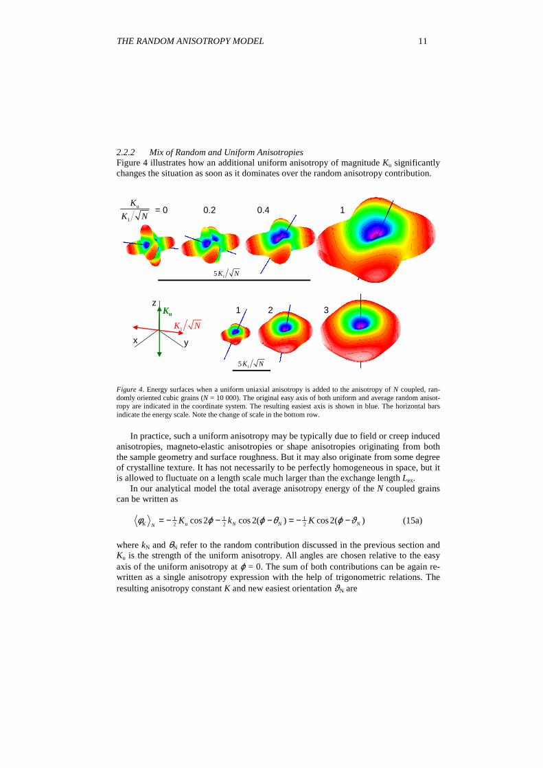
2.2.2 Mix of Random and Uniform AnisotropiesFigure 4 illustrates how an additional uniform anisotropy of magnitude Ku significantlychanges the situation as soon as it dominates over the random anisotropy contribution.

15K N

1 2 3

15K N

= 0 0.2 1u

1

KK N

0.4

x y

zKu

1K N

Figure 4. Energy surfaces when a uniform uniaxial anisotropy is added to the anisotropy of N coupled, ran-domly oriented cubic grains (N = 10 000). The original easy axis of both uniform and average random anisot-ropy are indicated in the coordinate system. The resulting easiest axis is shown in blue. The horizontal barsindicate the energy scale. Note the change of scale in the bottom row.

In practice, such a uniform anisotropy may be typically due to field or creep inducedanisotropies, magneto-elastic anisotropies or shape anisotropies originating from boththe sample geometry and surface roughness. But it may also originate from some degreeof crystalline texture. It has not necessarily to be perfectly homogeneous in space, but itis allowed to fluctuate on a length scale much larger than the exchange length Lex.

In our analytical model the total average anisotropy energy of the N coupled grainscan be written as

1 1 12 2 2cos 2 cos 2( ) cos 2( )K u N N NN

K k Kφ ϕ ϕ θ ϕ ϑ= − − − = − − (15a)

where kN and θN refer to the random contribution discussed in the previous section andKu is the strength of the uniform anisotropy. All angles are chosen relative to the easyaxis of the uniform anisotropy at ϕ = 0. The sum of both contributions can be again re-written as a single anisotropy expression with the help of trigonometric relations. Theresulting anisotropy constant K and new easiest orientation ϑN are

12 Giselher Herzer

2 2u u

12

2 cos 2sin 2

arctancos 2

N N N

N NN

u N N

K K k K kk

K k

θθϑ

θ

= + +

=+

(15b)

With similar arguments as in the previous section, the ensemble average of K follows as

22u u NK K f k= + (16)

where <kN> is the average random contribution given by Eq. (12a). The parameter fudenotes a correction arising from the randomly fluctuating cross term between the ran-dom and uniform anisotropy. It is a function of Ku/<K> which, in general, equals onefor Ku = 0 and evaluates to a constant value for Ku >> <kN>. It can be reasonably ap-proximated as fu ≈ 1 − cu (Ku/<K>)2 in lowest significant order. We find cu ≈ <cos²2θN>= 0.5 for our planar anisotropy model. A spherical distribution of random angles in-volves just more complicated expressions for the angular moments. From the numericalsimulations we find cu ≈ 0.5 for the uniaxial and cu ≈ 0.2 for the cubic case, i.e. ap-proximately cu ≈ β/2 in either case.

0.01 0.1 1 100.0

0.2

0.4

0.6

0.8

1.0

ϑ (ra

d)

Ku/<K1>

uniaxialcubic

easiestaxis

Ku ϑ

Figure 5. Numerical calculation of the average angle ϑ (:= arccos<|cos ϑ |>) between the easiest and the mac-roscopic easy axis as a function of the uniform anisotropy constant Ku normalized to the average anisotropyconstant <K1> := K1/N1/2 for randomly oriented cubic (full symbols) and uniaxial (open symbols) grains. Thedashed line is the limit for Ku = 0. The results represent averages over statistical ensembles with up to 4000sets of each N (= 4 to 220) grains; Ku was varied in the range Ku = 0.00125 to 0.64 K1.

As illustrated in Fig. 4, the easiest axis is rotated towards the macroscopic anisot-ropy axis as soon as Ku approaches and finally exceeds the order of the random contri-bution. Figure 5 supplements the average orientation of the easiest axis as a function ofKu/<K1>, for both uniaxial and cubic random anisotropies. Accordingly, the magneticmoments are forced to align more and more parallel, but this time as a consequence of

THE RANDOM ANISOTROPY MODEL 13

the uniform anisotropy. The decreasing angular dispersion ϑ 2 reduces the amount ofexchange energy. Accordingly, the averaged total free energy density is now given by

( )22 1ex 2A L Kφ ε α≈ ⋅ − , (17)

where ε = ϑ /θ is the average ratio between the easiest angle ϑ for Ku > 0 and the ran-dom angle θ. It is related to the anisotropy constants by

2 22Nf k Kεε = ⋅ . (18)

By definition, ε 2 equals one for Ku = 0. But it scales down as 1/N = (D/Lex)3 for domi-nating Ku, thus, modifying the scaling behavior of the exchange energy. The parameterfε denotes a correction from the anisotropy cross terms similar to fu in the average ani-sotropy constant. Like fu, it equals one for Ku = 0 and evaluates to a constant value forKu >> <kN>. It can be again reasonably approximated as fε ≈ 1 − cε (Ku/<K>)2 in lowestsignificant order. For our planar model we find cε ≈ <sin²2θN> = 0.5. For a sphericaldistribution of random angles, the numerical simulations yield cε ≈ 0.8 for both the uni-axial and cubic case.

The minimization of <φ> with respect to Lex again relates the renormalized ex-change length to the average anisotropy constant <K> in the usual form3, i.e. Lex =ϕ0(βA/<K>)1/2. The minimum energy <φ>min itself results as <φ>min ≈ (1− 3ε2/4)<φ K>min.

When the uniform anisotropy is dominating over the random contribution, the aver-age anisotropy constant evaluates as <K> – Ku ∝ 1/N. This changes the scaling behaviorof the random contribution from a D6 to a D3 law.

Figure 6 shows the corresponding result obtained by numerical simulations. Thenumerical results for the average anisotropy energies are very well described by thetheoretical relations. The theoretical estimate of the anisotropy angle is reasonable onlyfor Ku < <kN> and Ku > <kN>, but relatively crude in the intermediate range where Ku ≈<kN>. The corresponding fit is much better for random uniaxial anisotropies.

The figure actually shows an effective anisotropy constant Keff defined as the energydifference needed to rotate the magnetization from its easiest direction (1) into the mac-roscopically hard axis (3). This definition is introduced here because the average anisot-ropy constant <K> itself involves the hardest axis determined by Ku and the randomcontributions which is virtually inaccessible in experiment. Accordingly, Keff rather cor-responds to the experimental situation, i.e. to the area under the hysteresis loop whenmagnetizing the sample perpendicular to the uniform anisotropy axis starting from thedemagnetized state.

3 The literal procedure of minimization actually introduces minor corrections arising from the anisotropy crossterms. This causes ϕ0 to deviate slightly from the value given in Eq. (8) as a function of Ku/<K>. However,in view of the simplifying assumptions entering into the scaling analysis, we have discarded this nominalresult in order not to overdraw the simplified approach.

14 Giselher Herzer

Keff

Keff -Ku

0D L

2ϑ

6D

3D

K eff /K

1, ϑ

2

easiestaxis

(1)(3)

(2)Ku

ϑ

0.1 0.2 0.4 0.6 0.8 110-5

10-4

10-3

10-2

10-1

1

Figure 6. Effective anisotropy constant Keff (:= φK(3) − φK(1)) and angular dispersion ϑ 2 (:=arccos2<|cosϑ |>)for a cubic single-phase system as a function of the normalized grain size D/L0. The random anisotropies weresuperimposed with a uniaxial anisotropy of magnitude Ku = 0.01⋅K1. The symbols are the numerical averagesfor a statistical ensemble with 3300 sets of each N = 2 to 218 grains; the lines are the theory. The small opensquares supplement the results for Ku = 0 (Nmax = 220). The ratio D/L0 was calculated from the average anisot-ropy constant <K> as D/L0 = (βK1/<K>)1/2/N 1/3 which results by combining the relations for L0 and Lex with N= (Lex/D)3. It covers the relevant grain size range (D ≈ 4 – 40 nm) for typical iron based nanocrystalline mate-rials (L0 ≈ 40 nm).

The difference δK = Keff − Ku reflects the average dispersion δK of the anisotropyconstant due to the random fluctuations. It determines the coercivity which for domainwall displacements is approximately given by

ex

max

12

Wc

s s

LKHJ x J

γ δλ

∂≈ ≈

∂(19)

where γw = 4 (A/K)1/2 is the domain wall energy, Js the saturation magnetization and λthe fluctuation length of the anisotropies. For exchange coupled grains, the latter equalsto the exchange length, i.e. λ ≈ Lex. The coercivity is thus directly proportional to theanisotropy dispersion δK. Hence, we expect Hc ∝ D3 if Ku is dominating. A corre-sponding behavior was indeed observed by Suzuki et al. [6] e.g. for nanocrystallineFe91Zr7B2 in the range D ≈ 12 – 18 nm. If the random anisotropies are dominating, δK issimply proportional to the average anisotropy itself which results in Hc ∝ D6 as shownin Fig. 1. It is most instructive to study the corresponding arguments of Alben et al. [2]who arrive at the essentially same results for both situations.

More long-range anisotropy fluctuations on a scale λ > Lex can of course contributeto Hc as well. Actually, these more classical mechanisms play the dominant role in op-timized FeCuNbSiB alloys and overshadow the grain size dependence expected fromthe random contribution. Most relevant to this are surface roughness, magneto-elasticanisotropies as well as a distribution of anisotropies induced during annealing along theorientation of the magnetization in the domains at elevated temperatures.

THE RANDOM ANISOTROPY MODEL 15

The permeability µ, in general, depends upon the angle between the applied fieldand the uniform anisotropy like in the more classical case,. If the sample is magnetizedperpendicular to the uniform anisotropy axis µ is inversely proportional to the total ani-sotropy, i.e. µ ∝ 1/Keff, and, hence, grain size independent if Ku is dominating. If mag-netized parallel to the uniform axis it is determined by δK, i.e. µ ∝ 1/δK, with a corre-sponding grain size dependence. This distinction gets lost for dominating random an-isotropies and we arrive at the 1/D6 dependence shown in Fig. 1 since Keff = δK.

2.3 MATERIAL PARAMETERS

As pointed out earlier, the basic exchange length L0 remains an open parameter of thescaling analysis. From the formal point of view, the precise value of this length scale isultimately irrelevant for characterizing the scaling behavior of <K> with the structuralcorrelation lengths. I was therefore rather generous with respect to that issue in previouspublications where I put the pre-factors for L0 simply to one (cf. [3-6]). Similarly, thework of Alben et al. [2] should be also read generously with respect to the actual pre-factors.

However, from a practical point of view it is highly desirable to relate L0 to the ac-tual material parameters as close as possible. For this purpose we need to look moreclosely at the exchange interaction energy. The latter was simplified as <A(∇ m)2> =A(α /Lex)2 in order extract its scaling behavior. This actually involves two questions, i.e.:

1. What is the average exchange constant A for multi phase systems?2. What is the effective angle α between the easiest axis of exchange coupled regions?

The exchange constant A has to be ultimately understood as an effective averagevalue on the scale of the exchange length. However, as demonstrated by experiment, itis not a simple volume average. It is rather determined by the "weakest link" in the ex-change chain which, for example, is the amorphous intergranular phase in typical nano-crystallized materials [3]. Hence, it should result from some kind of "inverse averaging"of the local exchange constants, similar to the way how parallel resistors are adding. Weare leaving that theoretical issue open here and refer to the work of Suzuki et al. [7] whohave proposed so far the most reasonable physical approach to the problem. Instead, wesimply use the experimental value of the nanocrystallized material. The latter should bepreferred over the value for the crystalline phase which I originally used to estimate theaverage anisotropy constant for room temperature (cf. [3, 4]).

The parameter α is defined as α2:= <(Lex∇ m)2>. Accordingly, we need to estimatethe magnetization gradient between two neighboring regions of coupled grains. Let θdenote the smallest angle enclosed by the corresponding easy axis. We assume that themagnetization is rotating on a cone from one easy axis to the other easy axis in a stray-field free way similar to the situation in a domain wall (cf. [8]). This yields (∇ m)2 =sin2ϑ (∇ φ)2 where ϑ is the polar angle of the cone. The azimuth angle φ (= φ0...φ0+δφ)describes the rotation of the magnetization. From the geometry, δφ is given by cosδφ =(cosθ–cos2ϑ)/sin2ϑ where ϑ may be any angle between θ/2 to π/2. Like in a domainwall, the azimuth angle φ changes approximately linearly on the scale of Lex, i.e. (∇ φ)2 ≈(δφ/Lex)2. The minimum exchange energy results for a "flat cone", i.e. for ϑ = π/2. The

16 Giselher Herzer

effective angle α between the easiest axis is thus given by α = <θ 2>1/2. Statistically, theangles between the easy axis themselves are equivalent to the polar angles between theindividual easy axis and a macroscopic direction. Accordingly, <θ 2> can be calculatedby averaging over the angles θ of the easy directions nearest to the polar axis, similar tothe classical calculation of the remanence for multi particle systems (cf. [8]). The resultis α ≈ 1.068 for uniaxial and α ≈ 0.561 for cubic symmetry. For mixed symmetries αwill be determined by the symmetry of the dominating anisotropy contribution.

The cubic case actually needs some more reasoning: The random average results inonly one easiest magnetic axis, i.e. we would have the same value for α as for uniaxialanisotropies. Yet, there are a number of easy directions which still remind of the cubicsymmetry and which are energetically close together. The exchange plus anisotropyenergy can be ultimately minimized if the magnetization is parallel to any of these easyaxis. The latter can be of <100> or <111> type, irrespective of the sign of the local ani-sotropy constant K1. Accordingly we assumed <θ 2> = (<θ 2>100+<θ 2>111)/2.

In the preceding arguments, we considered Lex as the scale on which the magnetiza-tion is coherently rotating from the easy axis of one exchange coupled region to the easyaxis of the neighboring region. In contrast to this, we assumed the magnetic moments ofthe coupled grains to be oriented perfectly parallel in the arguments for the average ani-sotropy. This apparent ambiguity may be resolved as follows:

Let us think of a second scale L1 < Lex on which the magnetization is largely paral-lel. Both L1 and Lex are determined by the interplay of exchange and anisotropy energyand, hence, are proportional to each other. The minimum anisotropy energy on the scaleof L1 would be φK

min(L1) ≈ –K1⋅(D/L1)3/2. However, the corresponding easiest axis aredetermined by the local anisotropy fluctuations and, hence, are randomly oriented. Themagnetization cannot follow these random orientations along the scale of Lex due to thesmoothing effect of the exchange interaction. Consequently, the anisotropy is averagedout additionally and its average minimum density approaches φK

min(Lex) ≈ –K1⋅(D/Lex)3/2.Thus, the distinction between L1 and Lex gets lost, at least to a certain extent. Themechanism can be approximately confirmed for simplified model situations where thetotal energy can be minimized analytically. It thus appears legitimate to assume that theaverage over the random anisotropies of N grains with perfectly parallel magnetizationis approximately the same as the corresponding average for the case where we allow acoherent variation of the magnetization m over the same scale. Actually, the same con-clusion is obtained if we suppose that the variation of m on the scale of Lex is statisti-cally independent from the random orientation of the local easy axis. Possible correc-tions to this assumption would result in somewhat larger values of the parameter β or,vice versa, in somewhat smaller values for α. Yet this remains an uncertainty which stillhas to be clarified.

Table I summarize the results for a, β and ϕ0 obtained with the preceding argu-ments. Table II gives the corresponding estimate of the basic exchange length L0 fornanocrystalline FeCuNbSiB alloys together with some relevant material parameters. Butcaution, some of the reasoning behind these parameters is not free of some uncertain-ties. The numerical precision given in the tables is therefore apparent and only validwithin the corresponding assumptions. The values represent ultimately only a best guessand should be handled with the appropriate pre-caution.

THE RANDOM ANISOTROPY MODEL 17

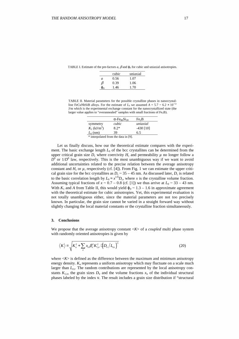
TABLE I. Estimate of the pre-factors a, β and ϕ0 for cubic and uniaxial anisotropies.

cubic uniaxiala 0.56 1.07β 0.39 1.06ϕ0 1.46 1.70

TABLE II. Material parameters for the possible crystalline phases in nanocrystal-line FeCuNbSiB alloys. For the estimate of L0 we assumed A = 5.7 − 6.2 × 10−12

J/m which is the experimental exchange constant for the nanocrystallized state (thelarger value applies to "overannealed" samples with small fractions of Fe2B).

α-Fe80Si20 Fe2Bsymmetry cubic uniaxialK1 (kJ/m3) 8.2* -430 [10]L0 (nm) 39 6.5* interpolated from the data in [9].

Let us finally discuss, how our the theoretical estimate compares with the experi-ment. The basic exchange length L0 of the bcc crystallites can be determined from theupper critical grain size Dc where coercivity Hc and permeability µ no longer follow aD6 or 1/D6 law, respectively. This is the most unambiguous way if we want to avoidadditional uncertainties related to the precise relation between the average anisotropyconstant and Hc or µ, respectively (cf. [4]). From Fig. 1 we can estimate the upper criti-cal grain size for the bcc crystallites as Dc ~ 35 – 45 nm. As discussed later, Dc is relatedto the basic correlation length by L0 ≈ x1/6Dc, where x is the crystalline volume fraction.Assuming typical fractions of x ~ 0.7 – 0.8 (cf. [1]) we thus arrive at L0 ~ 33 – 43 nm.With K1 and A from Table II, this would yield ϕ0 ~ 1.3 – 1.6 in approximate agreementwith the theoretical estimate for cubic anisotropies. Yet, this experimental evaluation isnot totally unambiguous either, since the material parameters are not too preciselyknown. In particular, the grain size cannot be varied in a straight forward way withoutslightly changing the local material constants or the crystalline fraction simultaneously.

3. Conclusions

We propose that the average anisotropy constant <K> of a coupled multi phase systemwith randomly oriented anisotropies is given by

( )32 2 2u 1, exK K x K D Lν ν ν ν

νβ= + ⋅∑ (20)

where <K> is defined as the difference between the maximum and minimum anisotropyenergy density. Ku represents a uniform anisotropy which may fluctuate on a scale muchlarger than Lex. The random contributions are represented by the local anisotropy con-stants K1,ν, the grain sizes Dν and the volume fractions xν of the individual structuralphases labeled by the index ν. The result includes a grain size distribution if “structural

18 Giselher Herzer

phase” refers to all grains with the same anisotropy constant K1,ν and the same grainssize Dν. The parameters βν mainly involve conventions used for defining the anisotropyenergy for different symmetries, but also include some statistical corrections in the or-der of 10% – 20%. They sharpen our previous results [3 – 6]. The final relation has beengeneralized to include mixed symmetries by weighing the structural phases with theirindividual symmetry moments βν. Numerical summations for a single phase systemresult in β ≈ 1 for uniaxial and β ≈ 0.4 for cubic symmetry. We have omitted less rele-vant corrections from anisotropy cross terms between the uniform anisotropy Ku and therandom contributions. The latter can be taken into account in lowest order by the sub-stitution β 2 → β 2⋅(1− 0.5 β (Ku/<K>)2).

The result is based on statistical concepts which apply as long as the average num-ber of coupled grains

( )3ex / 1N x L Dν ν ν= > (21)

is larger than one for each individual phase. Coupling so far only specifies that the mag-netization is parallel within the volume defined by the magnetic correlation length Lex.

If the coupling is dominated by exchange interaction, this magnetic correlationlength can be self-consistently related to average anisotropy constant <K> by

exL A K= ϕ . (22)

In the general case, the average anisotropy <K> has to be determined by iteration.Explicit solutions can be obtained in the limiting cases of a vanishing or dominatingmacroscopic anisotropy Ku. The results are

( )2

3

1, 0,K x K D Lν ν ν ν νν

β = ∑ (23)

for Ku = 0, and

( )31

u 1, u 0,2K K x K K D Lν ν ν ν νν

β≈ + ∑ (24)

if the uniform anisotropy is dominating over the random contributions. The latter is ac-companied by a change of the scaling behavior of the random anisotropy contributionfrom D6 to D3. In both relations

0, 0, 1,:L A Kν ν ν= ϕ with 0, :ν νβϕ = ϕ (25)

define the basic exchange lengths related to the local anisotropies of the individualstructural phases. The corresponding pre-factors are expected to be about ϕ0 ~ 1.5.

Figure 7 illustrates the expected grains size dependence of the average random ani-sotropy for typical Fe-based nanocrystalline alloys with a majority phase of bcc crystal-

THE RANDOM ANISOTROPY MODEL 19

lites. The figure basically sketches two situations which correspond to the optimizednanocrystalline state and the initial second stage of crystallization when small fractionsof Fe2B are precipitating (cf. [1]).

1 5 10 5010-4

10-3

10-2

10-1

1

101

102

103

104

D (nm)

<K>

(J/m

3 )

5% Fe2B: DFeB = 2 nm

25% amorph.

D6

D3

5% Fe2B: DFeB = 4 nm

5% Fe2B: DFeB = 6 nm

Figure 7. Theoretical estimate of the average anisotropy <K> for a system of randomly oriented crystallites ofbcc Fe80Si20 with grain size D and volume fraction x = 0.75. The crystallites are embedded in an amorphousmatrix where a small fraction (5%) of Fe2B with a size of 2 – 6 nm is assumed to precipitate. Only the randomanisotropy contributions are shown. The material parameters are given in Tables I and II. The atomic scaleanisotropy constant of the amorphous phase was assumed to be the same as that of Fe2B.

In the regime where the contribution of the bcc crystallites is dominating, the ex-pressions for <K> and Lex simplify drastically, i.e.

( )621 1 0:K K K x D Lβ β= = ⋅ (26)

( )3ex 0 0 /L L L D x= . (27)

The only modification compared to a single phase system is that the relations involvethe crystalline volume fraction x. Both <K> and Lex are hereby scaling with the volumefraction in the same way as with the crystalline volume D3

. The relations are identical tothose for exchange coupled crystallites diluted in an ideally soft magnetic matrix. Thecontribution of the amorphous phase is virtually negligibly small, although its local ani-sotropy has been assumed to be more than an order of magnitude higher than that of thebcc crystallites. This is related to the circumstance that the corresponding anisotropiesare fluctuating on the much shorter scale of atomic distances (Dam. ≈ 0.5 nm).

The condition Nν > 1 is always fulfilled for the amorphous matrix. For the crystal-lites it simplifies to

1/ 60D L x< . (28)

20 Giselher Herzer

The critical grain size below which the averaging process takes place is somewhat en-hanced due to the dilution effect4.

For the optimum nanocrystallized state with no boride precipitates, <K> is scalingwith D6 down to grain sizes of about 5 nm. The random anisotropy of the amorphousmatrix becomes only visible for very small grains resulting in a grain size independentanisotropy. However, the related coercivity (Hc ~ 0.001 A/m) is so small, that the situa-tion shown for small grain sizes in Fig. 7 remains academic. In real materials, whetheramorphous or nanocrystalline, the minimum Hc is ultimately determined by more longrange anisotropy fluctuations which have been not considered in the figure. The lowerlimit where there is no more benefit of reducing the grain size is ultimately located atgrain sizes of about 10 nm for typical FeCuNbSiB alloys (cf. Fig. 1).

Yet, a very small volume fraction of a phase with high anisotropy and a grain sizesomewhat larger than the atomic scale can change the picture significantly. This is il-lustrated in Fig. 7 assuming a small fraction of Fe2B precipitates with different grainsizes. The example explains at least qualitatively the familiar finding that Fe2B precipi-tates significantly deteriorate the soft magnetic properties although the grain size of thebcc crystallites may remain virtually unchanged (cf. Fig. 1). The transition regionswhere the average anisotropy of bcc grains starts to dominate can be approximatelycharacterized by a D3 law in a limited range of grain sizes. One can thus speculatewhether a D3 dependence of Hc, so far related to the presence of a uniform anisotropy,might be also attributed to an "improper" intergranular matrix in certain cases. Yet this,like many other details, still needs further investigation.

The focus of this review was on how to sum up random anisotropies. The essentialassumption hereby was that the magnetization is largely parallel over a sufficiently largenumber N of grains. The coupling mechanism hereby has not necessarily to be exchangeinteraction but could also be dipolar interaction. In the latter case "Lex" should be under-stood as magnetic correlation length which is not necessarily proportional to 1/<K>1/2

like it is for exchange interaction. But many of the arguments and results for the averageanisotropy still apply as long as we leave the relation between "Lex" and <K> open.

Dipolar interactions, without any doubt, become increasingly important when theexchange interaction between the crystallites is largely interrupted, e.g. when the amor-phous intergranular phase becomes paramagnetic (cf. [5]). It is still open how to incor-porate them correctly into the scaling analysis of the total energy.

Another open question for multi-phase systems is how to relate in general the effec-tive exchange constant A to the local material parameters. Suzuki's model [7] assumesthat the crystalline phase is completely surrounded by the amorphous phase. The latter,in many cases reflects the typical situation in nanocrystallized materials. But what is theappropriate model if, for example, the crystallites were only one or two atomic distancesapart or even were touching each other more or less frequently? The answer is not givenyet, while the arguments for averaging the individual anisotropies are still the same.

The problems of quantifying the effective exchange constant or the ferromagneticcorrelation length for dipolar interactions, thus, still provide profound theoretical chal-lenges which appear to be by far more complex than the statistical summation procedurefor the random anisotropies.

4 The somewhat different dilution effect (x1/4 instead of x1/6) given in [5] was related to the anisotropy fluctua-tions and not to average anisotropy <K>, which makes a difference for D > Lex.

THE RANDOM ANISOTROPY MODEL 21

References

1. Herzer, G. (1997) Nanocrystalline soft magnetic alloys, in K.H.J. Buschow (Ed), Handbook of MagneticMaterials Vol. 10, Elsevier Science, pp. 415-462

2. Alben, R., Becker, J.J. and Chi, M.C. (1978) Random anisotropy in amorphous magnets, J. Appl. Phys49, 1653-1658

3. Herzer, G. (1989) Grain structure and magnetism of nanocrystalline ferromagnets, IEEE Trans. Magn.25, 3327-3329

4. Herzer, G. (1990) Grain size dependence of coercivity and permeability in nanocrystalline ferromagnets,IEEE Trans. Magn. 26, 1397-1402

5. Herzer, G. (1995) Soft magnetic nanocrystalline materials, Scr. Metall. Mater. 33, 1741-17566. Suzuki, K., Herzer, G. and Cadogan, J.M. (1998) The effect of coherent uniaxial anisotropies on the

grain size dependence of coercivity in nanocrystalline soft magnetic alloys, J. Mag. Magn. Mater. 177-181, 949-950

7. Suzuki, K. and Cadogan, J.M. (1998) Random magnetocrystalline anisotropy in two-phase nanocrystal-line systems, Phys. Rev. B 58, 2730-2739

8. Chikazumi, S. and Charap, H. (1964) Physics of Magnetism, Robert E. Krieger Publishing Company,Malabar, Florida

9. Gengnagel, H. and Wagner, H. (1961) Magnetfeldinduzierte Anisotropie an FeAl- und FeSi-Einkristallen, Z. Angew. Phys. 8, 174 – 177

10. Iga, A., Tawara, Y. and Yanase, A. (1966) Magnetocrystalline anisotropy of Fe2B, J. Phys, Soc, Japan21, 404