The RealGas and RealGasH2O options of the TOUGHþ code for thesimulation of coupled fluid and heat flow in tight/shale gas systems

George J. Moridis a,n, Craig M. Freeman a,b

a Earth Sciences Division, Lawrence Berkeley National Laboratory, USAb Petroleum Engineering Department, Texas A&M University, USA

a r t i c l e i n f o

Article history:Received 10 April 2013Received in revised form14 September 2013Accepted 17 September 2013Available online 17 October 2013

Keywords:Numerical simulationFractured mediaMulticomponent flowCoupled flow and heat flowShale gasReal gas mixture

a b s t r a c t

We developed two new EOS additions to the TOUGHþ family of codes, the RealGasH2O and RealGas.The RealGasH2O EOS option describes the non-isothermal two-phase flow of water and a real gasmixture in gas reservoirs, with a particular focus in ultra-tight (such as tight-sand and shale gas)reservoirs. The gas mixture is treated as either a single-pseudo-component having a fixed composition,or as a multicomponent system composed of up to 9 individual real gases. The RealGas option has thesame general capabilities, but does not include water, thus describing a single-phase, dry-gas system. Inaddition to the standard capabilities of all members of the TOUGHþ family of codes (fully-implicit,compositional simulators using both structured and unstructured grids), the capabilities of the two codesinclude coupled flow and thermal effects in porous and/or fractured media, real gas behavior, inertial(Klinkenberg) effects, full micro-flow treatment, Darcy and non-Darcy flow through the matrix andfractures of fractured media, single- and multi-component gas sorption onto the grains of the porousmedia following several isotherm options, discrete and fracture representation, complex matrix–fracturerelationships, and porosity–permeability dependence on pressure changes. The two options allow thestudy of flow and transport of fluids and heat over a wide range of time frames and spatial scales not onlyin gas reservoirs, but also in problems of geologic storage of greenhouse gas mixtures, and of geothermalreservoirs with multi-component condensable (H2O and CH4) and non-condensable gas mixtures.

The codes are verified against available analytical and semi-analytical solutions. Their capabilities aredemonstrated in a series of problems of increasing complexity, ranging from isothermal flow in simpler1D and 2D conventional gas reservoirs, to non-isothermal gas flow in 3D fractured shale gas reser-voirs involving 4 types of fractures, micro-flow, non-Darcy flow and gas composition changes duringproduction.

Published by Elsevier Ltd.

1. Introduction

1.1. Background

The ever-increasing energy demand, coupled with the advent andadvances in reservoir stimulation technologies, has prompted anexplosive growth in the development of unconventional gasresources in the U.S. during the last decade. Tight-sand and shalegas reservoirs are currently the main unconventional resources, uponwhich the bulk of production activity is currently concentrating(Warlick, 2006). Production from such resources in the U.S. hasskyrocketed from virtually nil at the beginning of 2000, to 6% of thegas produced in 2005 (U.S. EIA, 2008), to 23% in 2010, and is expected

to reach 49% by 2035 (U.S. EIA, 2011). Production of shale gas isexpected to increase from a 2007 U.S. total of 1.4 TCF to 4.8 TCF in2020 (API, 2013). The ability to recover natural gas from shale gasformations has led to a dramatic increase in the estimate of the U.S.gas reserves, which increased by 35% from 2006 to 2008 (Mouawad,2009) and stood at 2000 TCF in 2009 (US DOE, 2009). In its AnnualEnergy Outlook for 2011, the US Energy Information Administration(EIA) more than doubled its estimate of technically recoverable shalegas reserves in the US from 353 TCF to 827 TCF by including datafrom recent drilling results in the Marcellus, Haynesville, and EagleFord shales (U.S. EIA, 2011). Note that the bulk of the gas productionfrom tight sands and shales has concentrated almost exclusively inNorth America (U.S. and Canada), and serious production elsewherein the rest world has yet to begin. This leads to justified expectationsthat gas production from such ultra-tight systems may be one of themain sources (if not the main source) of natural gas in the world fordecades to come, with obvious implications and benefits for nationaleconomies and national energy security.

Contents lists available at ScienceDirect

journal homepage: www.elsevier.com/locate/cageo

Computers & Geosciences

0098-3004/$ - see front matter Published by Elsevier Ltd.http://dx.doi.org/10.1016/j.cageo.2013.09.010

n Corresponding author. Tel.: þ1 510 486 4746; fax: þ1 510 486 5686.E-mail addresses: gjmoridis@lbl.gov,

george.moridis@pe.tamu.edu (G.J. Moridis).

Computers & Geosciences 65 (2014) 56–71

Nomenclature

A surface area, m2

b Klinkenberg parameter, PaB formation volume factor, surface volume/reservoir

volumebf fracture width, mc exponent of the Freundlich sorption isotherm, dimen-

sionless (see Eq. (6))ct total compressibility, Pa�1

CR heat capacity of the dry rock, J kg�1 K�1

cw water compressibility, Pa�1

DiK Knudsen diffusivity of species gi, m2 s�1

Dκβ multicomponent molecular diffusion coefficient of

component κ in phase β in the absence of a porousmedium, m2 s�1

Dije effective gas (binary) diffusivity of species gi in species

gj, m2 s�1

Ei the exponential integral functionFCD fracture conductivity, dimensionlessFβ the flow vector of phase β, kg m�2 s�1

Fκ, Fκβ the flow vector of component κ, and of component κ inphase β, kg m�2 s�1

g gravitational acceleration vector, m s�2

ff fracture void fraction, dimensionlessfs radiance emittance factor, dimensionlessh reservoir thickness, mhκβ specific enthalpy of component κ in phase β, J kg�1

Hi Henry's constant (factor) of species gi in H2O, PaHdep specific enthalpy departure of the gas mixture, J kg�1

Uisol specific enthalpy of dissolution of gas component gi in

H2O, J kg�1

Hβ specific enthalpy of phase β, J kg�1

Jκβ diffusive mass flux of component k in phase β,kg m�2 s�1

k permeability, m2 (mm2 for Cinco–Meng solution)kg Klinkenberg-adjusted permeability, m2

k1 absolute matrix permeability, m2

kf fracture permeability, m2

kiF kinetic coefficients of the Freundlich sorption iso-therm, s�1 (see Eq. (6))

KiF distribution coefficient of the Freundlich sorption

isotherm of gas gi, Pa�c

kL kinetic constant of the Langmuir sorption, s�1

kil kinetic coefficient of the linear sorption isotherm, s�1

(see Eq. (5))Kil distribution coefficient of the linear sorption isotherm

of gas gi, Pa�1

kθ composite thermal conductivity of the fluids-impregnated rock, W m�1 K�1

l fracture spacing, mmL Langmuir isotherm parameter, kg of gas/kg of matrix

(see Eq. (3))n number of normal sets of fractures, dimensionlessn the inward unit normal vectorNG number of gaseous components in the water–free gas

mixtureNi

D molar flux of component gi, mole/m2/sp pressure, Papb base pressure reference point for pseudo-pressure

computation, PaPcGA gas–water capillary pressure, PapD dimensionless pressure

pdc conversion factor (¼2π in SI units)pdg dry gas pressure, Papk Klinkenberg-adjusted pressure, PapL Langmuir isotherm parameter, Pa (see Eq. (3))pr pressure at radius r, Papv partial pressure of water vapor, Paq mass flow rate, kg s�1

qθ rate of heat addition/withdrawal, W kg�1

r radius, mrD dimensionless radiusre outer boundary radius, mrw wellbore radius, mt time, sT temperature, KtD dimensionless timeui ideal part of specific internal energy of sorbed gas

component gi, J kg�1

(ui)n total specific internal energy of sorbed gas componentgi, including departure effects, J kg�1

Udep specific internal energy departure of the gas mixture,J kg�1

Uisol specific internal energy of dissolution of gas compo-

nent gi in H2O, J kg�1

Uβ specific internal energy of phase β, J kg�1

vβ flow velocity of phase β, m s�1

V, Vn the volume and volume of subdomain n, respectively,m3

Vp pore volume, m3

xf fracture half-length, mZ gas compressibility factor, dimensionless

Greek symbols

α block shape factor, 1/m2

αK Knudsen-related parameter (see Eq. (29))β denotes phases, β¼A, Gββ parameter for Forchheimer flow of phase β

(See Eq. (15)γ permeability reduction factor, dimensionlessΓn the surface of subdomain n [m2],δ fracture aperture, mκ denotes the component κλ Warren and Root interporosity flow parameter,

dimensionlessλ mean free path of gas molecules, mμ viscosity, Pa-sτG gas tortuosity, dimensionlessϕ porosity, dimensionlessΦβ total pressure, Pa (see Eq. (11))ψ pseudo-pressure (see Eq. (28))Ψi mass of sorbed component gi per unit mass of

rock, kg/kgω Warren and Root storativity ratio, dimensionless

Subscripts

0 denotes initial conditionsA aqueousabs implies that the property reflects an absolute media

valuecont implies that the property reflects an equivalent

continuum-adjusted value

G.J. Moridis, C.M. Freeman / Computers & Geosciences 65 (2014) 56–71 57

The importance of tight-sand and shale reservoirs as energyresources necessitate the ability to accurately estimate reservesand to evaluate, design, manage and predict production from suchsystems over a wide range of time frames and spatial scales.Modeling and simulation play a key role in providing the neces-sary tools for these activities. However, these reservoirs presentchallenges that cannot be easily (if at all) handled by conventionalgas models and simulators: they are characterized by extremelylow permeabilities (often in the nD¼10�21 m2 range), have nativefractures that interact with the fractures created during thereservoir stimulation and with the matrix to result in verycomplicated flow regimes and patterns that very often do notfollow Darcy's Law, have pores of such small dimensions thatinterfere with the Brownian motion of the gas molecules (thusrendering standard advection-diffusion approaches irrelevant, andrequiring accounting for Knudsen diffusion and special formula-tions of multi-component diffusion), exhibit highly non-linearbehavior, have large amounts of gas sorbed onto the grains ofthe porous media in addition to gas stored in the pores, and mayexhibit unpredictable geomechanical behavior such as the evolu-tion of secondary fractures (Kim and Moridis, 2013) that mayfurther complicate an already complex flow regime.

Several analytical models have been proposed to predict flowperformance, and numerical studies have been conducted toanalyze production from these ultra-tight reservoirs. Most of thesestudies have assumed idealized and regular fracture geometries,and include significant simplifying assumptions. Among the var-ious analytical and semi-analytical solutions that have beenproposed to model flow in shale-gas and tight-gas reservoirs, theearly work of Gringarten (1971) and Gringarten et al. (1974)described the simplified flow through domains involving a singlevertical fracture and a single horizontal fracture. More accuratesemi-analytical models for single vertical fractures were devel-oped later (e.g., Blasingame and Poe Jr., 1993). Prior to thedevelopment of models for multiply-fractured horizontal wells(Medeiros et al., 2006), it was common practice to represent thesemultiple fractures with an equivalent single fracture. Morerecently, several other analytical and semi-analytical models havebeen developed (Bello and Wattenbarger, 2008; Mattar, 2008;Anderson et al., 2010), but these, despite their speed, cannotaccurately handle the very high nonlinear aspects of shale-gasand tight-gas reservoirs, cannot describe complex domain geome-tries, and cannot accurately capture gas sorption and desorptionfrom the matrix (a non-linear process that does not lend itself toanalytical solutions), multiphase flow, unconsolidation, andseveral non-ideal and complex fracture networks (Houze et al., 2010).

The importance of such ultra-tight reservoirs and the short-comings of the analytical and semi-analytical models have led tothe development of numerical reservoir simulators that address theparticularities of these systems. Miller et al. (2010) and Jayakumaret al. (2011) used numerical simulation to history-match andforecast production from two different shale-gas fields. Cipollaet al., (2009), Freeman (2010), Moridis et al., (2010) and Freemanet al., (2009; 2013) and conducted numerical sensitivity studies toidentify the most important mechanisms and factors that affectshale-gas reservoir performance. Powerful commercial simulatorswith specialized options for shale gas analysis such as GEM (CMG,2013) and ECLIPSE For Unconventionals (SLB, 2013) have becomeavailable. While these address the most common features ofunconventional and ultra-tight media, they are designed primarily

for large-scale production evaluation at the reservoir level andcannot be easily used for scientific investigations of micro-scaleprocesses and phenomena in the vicinity of fractures.

1.2. The TOUGHþ family of codes

TOUGHþ is a family of public domain codes developed at theLawrence Berkeley National Laboratory (Moridis et al., 2008) thatare a successor to the TOUGH2 (Pruess et al., 1991) family of codesfor multi-component, multiphase fluid and heat flow. It is writtenin standard FORTRAN 95/2003 to take advantage of all the object-oriented capabilities and the enhanced computational features ofthat language. It employs dynamic memory allocation, follows thetenets of Object-Oriented Programming (OOP), and involvesentirely new data structures and derived data types that describethe objects upon which the code is based. The TOUGHþ code isbased on a modular structure that is designed for maximumtraceability and ease of expansion.

TOUGHþ is a family of codes developed at the LawrenceBerkeley National Laboratory (Moridis et al., 2008) that are asuccessor to the TOUGH2 (Pruess et al., 1991) family of codes formulti-component, multiphase fluid and heat flow. It is written instandard FORTRAN 95/2003 to take advantage of all the object-oriented capabilities and the enhanced computational features ofthat language. It employs dynamic memory allocation, follows thetenets of Object-Oriented Programming (OOP), and involvesentirely new data structures and derived data types that describethe objects upon which the code is based. The TOUGHþ code isbased on a modular structure that is designed for maximumtraceability and ease of expansion.

1.3. Objectives and features

The main objective of this study was to develop numericalcapabilities allowing the description of a wide range of processesinvolved in the non-isothermal flow through the spectrum ofnatural gas reservoirs in geologic systems, including tight-gas andshale-gas reservoirs with natural and/or induced fractures.A particular focus is the incorporation of capabilities to describeprocess and phenomena occurring during the non-isothermal flowof real gases in fractured ultra-tight reservoirs, including non-Darcy flow, Knudsen and multi-component diffusion, and interac-tions of rock matrix with both discrete fractures with generalizedfracture effect concepts such as dual- and multi-porosity (Warrenand Root, 1963), dual-permeability, and multiple interactive con-tinua (Pruess, 1983).

To that end, we developed two new EOS additions to theTOUGHþ family of codes: the RealGasH2O and RealGas options(hereafter referred to as TþGW and TþG, respectively) for thedescription of two-phase (aqueous and gas) and single-phase (dry-gas) flow through complex geologic media, respectively.The TþGW and TþG codes account for practically all knownprocesses and phenomena, involve a minimum of assumptions,and are suitable for scientific investigations at any spatial (fromthe sub-mm scale in the vicinity of the fracture surface to thereservoir scale) and temporal scales, thus allowing insights intothe system performance and behavior during production.

In addition to all the standard capabilities common to theTOUGH2 (Pruess et al., 1999) and TOUGHþ (Moridis et al., 2008)family of codes, the physics and thermodynamics of mass and heat

f fractureG gasm matrix

pore indicates pore-associated propertyr denotes a reference statew denotes a well (source or sink)

G.J. Moridis, C.M. Freeman / Computers & Geosciences 65 (2014) 56–7158

flow through porous media in these two options include the mostrecent developments in the fields, and account for practically allknown processes. The new capabilities can provide solutions to theproblem of prediction of gas production from the entire spectrumof gas-bearing reservoirs, but also of any reservoir involving waterand gas mixtures of up to nine components. Of particular interestare applications to ultra-tight reservoirs (including tight-sandand shale reservoirs), the numerical simulation of which mayinvolve unstructured grids, extremely fine domain discretization,complex fracture–matrix interactions in several subdomains of theproducing system, Darcy and non-Darcy flow, single- and multi-component sorption following a variety of isotherm options, andcoupled thermophysical phenomena and processes.

Although this paper focuses mainly on problems of hydrocar-bon gas flow through tight reservoirs, it is important to indicatethat the TþGW code is fully applicable to a wide variety of otherproblems, including the study of the geological storage of green-house gas mixtures, and of geothermal reservoirs with multi-component non-condensable gas mixtures.

2. Code description

The ensuing discussion focuses on the description of theTþGW code describing the two-phase flow problem of an aqueousand a gas phase flow through a geologic system. The TþG code isentirely analogous, differing only in the omission of water as amass component, thus solving the much simpler problem ofsingle-phase, dry-gas flow and production.

2.1. Fundamental equations of mass and energy balance

A non-isothermal fractured tight-gas or shale-gas system canbe fully described by the appropriate mass balance equations andan energy balance equation. The following components κ, corre-sponding to the number of equations, are considered: κ¼gi, i.e.,the various gaseous components (compounds) i constituting thenatural gas (i¼1, …, NG, NGZ1); water (w), and heat (θ), treated asa pseudo-component. The following nine gaseous components arecurrently available to TþGW and TþG: CH4, C2H6, C3H8, C4H10,CO2, H2S, O2, N2 and H2, all of which except CO2 are treated as non-condensable. Note that in TþGW it is possible to treat a real gasmixture of constant composition (i.e., with non-variant molefractions Yi) as a single pseudo-component, the properties of whichvary with the pressure P and temperature T.

Following Pruess et al. (1999), mass and heat balance consid-erations in every subdomain (gridblock) into which the simulationdomain is been subdivided by the integral finite difference methodin TOUGHþ dictates that

ddt

ZVn

Mκ dV ¼ZΓn

Fκ Un dtþZVn

qκ dV ð1Þ

where V and Vn are the volume and volume of subdomain n [m3];Mκ is the mass accumulation term of component κ [kg m�3]; A andΓn are the surface area and surface of subdomain n [m2], respec-tively; Fκ is the flow vector of component κ [kg m�2 s�1]; n is theinward unit normal vector; qκ is the source/sink term of compo-nent κ [kg m�3 s�1]; and t is the time [s].

2.1.1. Mass accumulation termsUnder the two-phase (aqueous and gas) flow conditions

described by TþGW, the mass accumulation terms Mk for themass components κ in Eq. (1) are given by

∑β � A;G

ϕSβρβXκβ þ δΨ ð1�ϕÞρRΨ i ð2Þ

where κ�w; gi; i¼ 1; :::;NG; ϕ is the porosity [dimensionless]; ρβ isthe density of phase β [kg m�3]; Sβ is the saturation of phase β[dimensionless]; Xκ

β is the mass fraction of component in phase β[kg/kg]; ρR is the rock density [kg m�3]; Ψi is the mass of sorbedcomponent gi per unit mass of rock [kg/kg]; and δΨ¼0 for non-sorbing media (including tight-gas systems) that are usuallydevoid of substantial organic carbon, while δΨ¼1 in gas-sorbingmedia such as shales.

The first term in Eq. (2) describes fluid mass stored in the pores,and the second the mass of gaseous components sorbed onto theorganic carbon (mainly kerogen) content of the matrix of theporous medium. The latter is quite common in shales. Althoughgas desorption from kerogen has been studied extensively incoalbed CH4 reservoirs, and several analytic/semi-analytic modelshave been developed for such reservoirs (Clarkson and Bustin,1999), the sorptive properties of shale are not necessarily analo-gous to coal (Schettler and Parmely, 1991).

2.1.2. Gas sorption termsThe most commonly used empirical model describing sorption

onto organic carbon in shales is analogous to that used in coalbedmethane and follows the Langmuir isotherm that, for a single-component gas, is described by

Ψ i ¼ pdGmLpdG þpL

for ELaS

dΨ i

dt ¼ kLpdGmLpdG þpL

�Ψ i� �

for KLaS

8<: ð3Þ

where pdG is the dry gas pressure (pdG¼pG�pv, where pv is thepartial pressure of the water vapor), ELaS indicates EquilibriumLangmuir Sorption, and KLaS denotes Kinetic Langmuir Sorption.The mL term in Eq. (3) describes the total mass storage ofcomponent gi at infinite pressure (kg of gas/kg of matrix material),pL is the pressure at which half of this mass is stored (Pa), and kL isa kinetic constant of the Langmuir sorption (1/s). In most studiesapplications, an instantaneous equilibrium is assumed to existbetween the sorbed and the free gas, i.e., there is no transientlag between pressure changes and the corresponding sorption/desorption responses and the equilibrium model of Langmuirsorption is assumed to be valid. Although this appears to be agood approximation in shales (Gao et al., 1994) because of the verylow permeability of the matrix (onto which the various gascomponents are sorbed), the subject has not been fully investi-gated. For multi-component gas, Eq. (3) becomes

Ψ i ¼ pdGBimi

Lϒi

1þpdG∑iBiϒ i for ELaS

dΨ i

dt ¼ kiLpdGB

imiLϒ

i

1þpdG∑iBiϒ i �Ψ i

!for KLaS

8>>>><>>>>:

ð4Þ

where Bi is the Langmuir constant of component gi in 1/Pa (Panand Connell, 2009), and Yi is the dimensionless mole fraction ofthe gas component i in the water-free gas phase. Note that theTþGW and TþG codes offer the additional options of linear andFreundlich sorption isotherms (equilibrium and kinetic). For eachgas component gi, these are described by the following equations:

Ψ i ¼ Kilp

i for ELiSdΨ i

dt ¼ kilðKilp

i�Ψ iÞ for KLiS

8<: ð5Þ

Ψ i ¼ KiF ðpiÞc for EFS

dΨ i

dt ¼ kiF ½KiF ðpiÞc�Ψ i� for KFS

8<: ð6Þ

where ELiS and KLiS denote equilibrium and kinetic linear sorp-tion, respectively; EFS and KFS denote equilibrium and kineticFreundlich sorption, respectively; Ki

l and KiF are the distribution

G.J. Moridis, C.M. Freeman / Computers & Geosciences 65 (2014) 56–71 59

coefficients of the ELiS and EFS sorption isotherms of gas compo-nent i, respectively; pi is the partial pressure of gi; kil and kiF are thekinetic coefficients of the ELiS and EFS sorption isotherms of gi,respectively; and c is the exponent of the Freundlich sorptionisotherm.

2.1.3. Heat accumulation termsThe heat accumulation term includes contributions from the

rock matrix and all the phases, and is given by the equation

Mθ ¼ð1�ϕÞρR

R TTr CRðTÞdTþ

∑β ¼ A;G

ϕSβρβUβþδΨ ð1�ϕÞρR ∑NG

i ¼ 1uiΨ i

8>><>>: ð7Þ

where CR¼CR(T) is the heat capacity of the dry rock [J kg�1 K�1];Uβ is the specific internal energy of phase β [J kg�1]; (ui)* is thespecific internal energy of sorbed gas component gi, includingdeparture effects [J kg�1]; T is the temperature [K]; and Tr is areference temperature [K]. The specific internal energy of thegaseous phase is a very strong function of composition, is relatedto the specific enthalpy of the gas phase HG, and is given by

UG ¼ ∑κ ¼ w;giði ¼ 1;NGÞ

XκGu

κþUdep ¼HG�PρG

� �ð8Þ

where uκ is the specific internal energy of component κ in thegaseous phase, and Udep is the specific internal energy departure ofthe gas mixture [J kg�1]. The internal energy of the aqueous phaseaccounts for the effects of gas and inhibitor solution, and isestimated from

UA ¼ XwA u

wþ ∑NG

i ¼ 1Xgi

A ðuiþUisolÞ ð9Þ

where uw and ui are the ideal parts of the specific internal energiesof H2O and of natural gas component gi at the p and T conditions ofthe aqueous phase, respectively, and Ui

sol are the specific internalenergies of dissolution of the gas component gi in H2O (obtainedfrom tables). Note that the reference state for all internal energyand enthalpy computations are p¼101,300 Pa and T¼273.15 K(0 1C).

2.1.4. Fluid flux termsThe mass fluxes of water and of the gaseous components

include contributions from the aqueous and gaseous phases, i.e.,

Fκ ¼ ∑β � A;G

Fκβ; κ�w; gi; i¼ 1; :::;NG ð10Þ

For phase β, Fκβ ¼ XκβFβ . In TþGW and TþG, there are three options

to describe the phase flux Fβ . The first is the standard Darcy's law,i.e.,

Fβ ¼ ρβ � kkrβμβ

∇Φβ

" #¼ ρβvβ; ∇Φβ ¼∇pβ�ρβg; ð11Þ

where k is the rock intrinsic permeability [m2]; krβ is the relativepermeability of phase β [dimensionless]; μβ is the viscosity ofphase β [Pa s]; pβ is the pressure of phase β [Pa]; and g is thegravitational acceleration vector [m s�2]. In TþGW, the relation-ship between the aqueous and the gas pressures, pA and pG,respectively, is given by pA¼pGþPcGA, where PcGA is the gas–watercapillary pressure [Pa]. The krβ and PcGA options are the standardones available in the TOUGH2 and TOUGHþ family of codes(Pruess et al., 1999; Moridis et al., 2008).

The mass flux of component κ in the gas phase incorporatesadvection and diffusion contributions, and is given by

FκG ¼ 1þ bPG

� �ρGvGX

κG�ϕSGτGD

κGρG∇X

κG|fflfflfflfflfflfflfflfflfflfflfflffl{zfflfflfflfflfflfflfflfflfflfflfflffl}

� JκG

; ð12Þ

where b is the Klinkenberg (1941) b-factor accounting for gasslippage effects [Pa], the term JκG is the diffusive mass flux ofcomponent κ in the gas phase [kg m�2 s�1], Dκ

G is the multi-component molecular diffusion coefficient of component κ in thegas phase in the absence of a porous medium [m2 s�1], and τG isthe gas tortuosity [dimensionless].

The Klinkenberg b-factor is either provided as input, or iscomputed using the relationship proposed by Jones (1972) as

bbr

¼ kkr

� ��0:36

ð13Þ

where the subscript r denotes a reference medium with a knownb-factor and k, such as those listed by Wu et al. (1998). There areseveral methods to compute τG in the TþGW and TþG codes,including the Millington and Quirk (1961) model.

The diffusive mass fluxes of the water vapor and the natural gascomponents are related through the relationship of Bird et al. (2007)

JwG þ ∑NG

i ¼ 1Jg

i

G ¼ 0; ð14Þ

which ensures that the total diffusive mass flux of the gas phase iszero with respect to the mass average velocity when summed overthe components. Then the total mass flux of the gas phase is theproduct of its velocity and density.

If the flow is non-Darcian, then the equation Fβ ¼ ρβvβ stillapplies, but vβ is now computed from the solution of the quadraticequation

∇Φβ ¼ � μβkkrβ

vβþββρβvβjvβj�;

�ð15Þ

in which ββ is the “turbulence correction factor” (Katz et al., 1959).The quadratic equation in Eq. (14) is the general momentum-balance Forcheimer equation (Forchheimer, 1901; Wattenbargerand Ramey, 1968), and incorporates laminar, inertial and turbulenteffects. This is the second option. The solution then is

vβ ¼2∇Φβ

ðμβ=kkrβÞþffiffiffiffiffiffiffiffiffiffiffiffiffiffiffiffiffiffiffiffiffiffiffiffiffiffiffiffiffiffiffiffiffiffiffiffiffiffiffiffiffiffiffiffiffiffiffiðμβ=kkrβÞ2þ4ββρj∇Φβj

q ; ð16Þ

and vβ from Eq. (15) is then used in the equations of flow (11) and(12). TþGW and TþG offer 13 options to compute ββ, several ofwhich are listed in Finsterle (2001). The third option follows theapproach of Barree and Conway (2007), as described by Wu et al.(2011), which involves a different formulation of ∇Φβ .

2.1.5. Heat flux termsThe heat flux accounts for conduction, advection and radiative

heat transfer, and is given by

Fθ ¼ �kθ∇Tþ f ss0∇T4þ ∑

β � A;GHβFβ ð17Þ

where kθ is a representative thermal conductivity of the reservoirfluids-impregnated rock [W m�1 K�1]; hβ is a specific enthalpy ofphase β [J kg�1]; fs is the radiance emittance factor [dimension-less]; s0 is the Stefan–Boltzmann constant [5.6687�10�8 Jm�2 K�4]. The specific enthalpy of the gas phase is computed as

HG ¼ ∑κ � w;gi

XκGh

κGþHdep ð18Þ

where hKG is the specific enthalpy of component κ in the gaseous

phase, and Hdep is the specific enthalpy departure of the gas

G.J. Moridis, C.M. Freeman / Computers & Geosciences 65 (2014) 56–7160

mixture [J kg�1]. The specific enthalpy of the aqueous phase isestimated from

HA ¼ XwA h

wA þ∑

iXgi

A ðhgi

A þHgi

solÞ ð19Þ

where hwA and hgi

A are the specific enthalpies of H2O and of thenatural gas components in the aqueous phase, respectively, andHgi

sol is the specific enthalpy of dissolution [J kg�1] of gas compo-nent gi in the aqueous phase.

2.1.6. Source and sink termsIn sinks with specified mass production rate, withdrawal of the

mass component κ is described by

qκ ¼ ∑β � A;G

Xκβqβ ; κ¼w; gi ði¼ 1; :::;NGÞ ð20Þ

where qβ is the production rate of the phase β [kg m�3]. For aprescribed production rate, the phase flow rate qβ is determinedfrom the phase mobility at the location of the sink. For sourceterms (well injection), the addition of a mass component κ occursat desired rates. The contribution of the injected or producedfluids to the heat balance of the system are described by

qθ ¼ ∑β ¼ A;G

qβHβ; ð21Þ

where qθ is the rate of heat addition or withdrawal in the course ofinjection or production, respectively (W/kg).

2.1.7. p- and T-dependence of ϕ and kThe effect of pressure change on the porosity of the matrix is

described by two options. The first involves the standard expo-nential equation

ϕ¼ ϕr exp½αpðp�prÞþαT ðT�TrÞ� ð22Þ

where αT is the thermal expansivity of the porous medium (1/K)and αp is the pore compressibility (1/Pa), which can be either afixed number or a function of pressure (Moridis et al., 2008).A second option describes the p-dependence of ϕ as a polynomialfunction of p. The ϕ–k relationship is described by the generalexpression of Rutqvist and Tsang (2002) as

kkr

¼ exp γϕ

ϕr�1

� �� ð23Þ

where γ is an empirical permeability reduction factor that rangesbetween 5 (for soft unconsolidated media) and 29 (for lithified,highly consolidated media). Note that the equations describedhere are rather simple and apply to matrix ϕ and k changes whenthe changes in p and T are relatively small. These equations are notapplicable when large pressure and temperature changes occur inthe matrix, cannot describe the creation of new (secondary)fractures and cannot describe the evolution of the characteristicsof primary and secondary fractures (e.g., aperture, permeability,extent, surface area) over time as the fluid pressures, the tem-peratures, the fluid saturations and the stresses change. For suchproblems, it is necessary to use the TþM model (Kim and Moridis,2013) that couples the flow-and-thermal-process TþRW simula-tor discussed here with the ROCMECH geomechanical code. Thiscoupled model accounts for the effect of changing fluid pressures,saturations, stresses, and temperatures on the geomechanicalregime and provides an accurate description of the evolution ofϕ and k over the entire spectrum of p and T covered during thesimulation.

2.2. Physical–chemical processes

2.2.1. Micro-flowKnudsen diffusion and Dusty Gas model. For ultra-low perme-

ability media (such as tight sands and shales) and the resultingmicro-flow processes, the Klinkenberg b-factor for a single-component or pseudo-component gas in TþGW and TþG iscomputed by the method of Florence et al. (2007) and Freemanet al. (2011) as

bPG

¼ ð1þαKKnÞ 1þ 4Kn

1þKn

� ��1; ð24Þ

where Kn is the Knudsen diffusion number (dimensionless), whichcharacterizes the deviation from continuum flow, accounts for theeffects of the mean free path of gas molecules λ being on the sameorder as the pore dimensions of the porous media, and iscomputed from Freeman et al. (2011) as

Kn ¼ λ

rpore¼ μG

2:81708pG

ffiffiffiffiffiffiffiffiffiffiffiffiffiπRT2M

ϕ

k

r; ð25Þ

with M being the molecular weight and T the temperature (K). Theterm aK in Eq. (24) is determined from Karniadakis and Beskok(2001) as

αK ¼ 12815π2

tan �1ð4K0:4n Þ; ð26Þ

For simplicity, we have omitted the superscript i in Eqs. (23)–(26).The Knudsen diffusion can be very important in porous mediawith very small pores (on the order of a few micrometers orsmaller) and at low pressures. For a single gas pseudo-component,the properties in Eq. (26) are obtained from an appropriate equationof state for a real-gas mixture of constant composition Yi. TheKnudsen diffusivity DK [m2/s] can be computed as (Civan, 2008;Freeman et al., 2011)

DK ¼ 4ffiffiffiffiffiffikϕ

p2:81708

ffiffiffiffiffiffiffiffiffiπRT2M

ror DK ¼ kb

μGð27Þ

For a multicomponent gas mixture that is not treated as asingle pseudo-component, ordinary Fickian diffusion must betaken into account as well as Knudsen diffusion. Use of theadvective–diffusive flow model (Fick's law) should be restrictedto media with kZ10�12 m2; the dusty-gas model (DGM) is moreaccurate at lower k (Webb and Pruess, 2003). Additionally, DGMaccounts for molecular interactions with the pore walls in theform of Knudsen diffusion. Shales may exhibit a permeability k aslow as 10�21 m2, so the DGM described below is more appropriatethan the Fickian model (Webb and Pruess, 2003; Doronin andLarkin, 2004; Freeman et al., 2011):

∑NG

j ¼ 1;ja i

YiNjD�YjNi

D

Dije

� NiD

DiK

¼ pi∇Yi

ZRTþ 1þ kp

μGDiK

!Yi∇pi

ZRTð28Þ

where NiD is the molar flux of component gi [mole m�2 s�1], Dij

e isthe effective gas (binary) diffusivity of species gi in species gj, andDiK is the Knudsen diffusivity of species gi.

2.2.2. Gas solubilityThere are two options for estimating the solubility of a gas i

into the aqueous phase in TþGW. The first (and simpler one) isbased on Henry's Law, described by the relationship

pi ¼HiXiA; ð29Þ

where Hi [Pa] a T-dependent, species-specific factor referred to asHenry's factor (as opposed to its customary name as Henry'sconstant). TþGW includes a library of fast parametric relation-ships of Hi¼Hi(T) that cover a wide range of T and are applicableover a wide range of p, and this is the preferred option if a single

G.J. Moridis, C.M. Freeman / Computers & Geosciences 65 (2014) 56–71 61

gas component or pseudo-component is involved. The secondoption is based on the equality of fugacities in the aqueous and thegas phase, involves the chemical potentials of the various speciesin solution, and is applicable when p is very high, when there issignificant dissolved species interaction and/or dissolved salts (notthe case in TþRW, which does include an equation for salts).

2.2.3. Thermophysical propertiesThe water properties in the TþGW code are obtained from

steam table equations (IFC, 1967), as implemented in othermembers of the TOUGH family of codes (Pruess et al., 1999;Moridis et al., 2008), and cover a wide pressure and temperaturerange (from 10�4 MPa to 103 MPa, and from 235 K to 1273 K).

All the real gas properties in TþG and TþGW are computedfrom one of the three available options of cubic equations of state(EOS) – i.e., the Peng and Robinson (1976), the Redlich–Kwong(1949) and the Soave (1972) EOS – that were implemented byMoridis et al. (2008). The gas property package computes thecompressibility, density, fugacity, specific enthalpy and internalenergy (ideal and departure) of pure gases and gas mixtures over avery wide range of pressure and temperature conditions. Addi-tionally, the package uses the cubic equations of state to computethe gas viscosity and thermal conductivity using the method ofChung et al. (1988), and binary diffusivities from the method ofFuller et al. (1966) and Riazi and Whitson (1993). In addition to thestandard cubic equation of state, the thermodynamics of theTþGW and TþG package include a complete phase diagram ofCO2 (from liquid to gas to supercritical gas, and the correspondingthermophysical properties) that is based on a modification of theapproach in the ECO2M package (Pruess, 2011) of TOUGH2 (Pruesset al., 1999).

3. The solution approach

Following the standard approach in the TOUGH (Pruess et al.,1999) and TOUGHþ (Moridis et al., 2008) family of codes, thecontinuum Eq. (1) is discretized in space using the Integral FiniteDifference (IFD) method (Edwards, 1972; Narasimhan et al., 1978).The space discretization approach used in the IFD method and thedefinition of the geometric parameters are illustrated in Fig. 1.Note that, as Fig. 1 indicates, the IFD method is not limited tostructured (regular) grids, but is directly applicable to any irregu-larly shaped subdomains (unstructured grid) m and n as long asthe line Dnm connecting the centers of gravity between twogridblocks m and n is perpendicular to their common area Amn.

Of particular importance to the description of flow throughfractured media (as is invariably the case in tight reservoirs) in theTþG and TþGW codes is the availability of the method of MultipleInteracting Continua (MINC) (Pruess and Narasimhan, 1982, 1985;

Pruess, 1983). This method allows the accurate description ofcoupled fluid and heat flows with steep gradients at the frac-ture–matrix interfaces by appropriate subgridding of the matrixblocks. The MINC concept is based on the notion that changes influid pressures, temperatures, and phase compositions due to thepresence of sinks and sources (production and injection wells) willpropagate rapidly through the fracture system, while invading thetight matrix blocks only slowly. Therefore, changes in matrixconditions will (locally) be controlled by the distance from thefractures. Fluid and heat flow from the fractures into the matrixblocks, or from the matrix blocks into the fractures, can then bemodeled by means of one-dimensional strings of nested gridblocks.

The resulting discretized equations are expressed in residualform, are then linearized by the Newton–Raphson method and aresolved fully implicitly. The resulting Jacobian is solved in thestandard approach used in all TOUGH applications (Pruess et al.,1999). In TþG, the primary variables that constitute the solutionvector are pG, Yi (i¼1,…, NG), and T; in TþGW, the primaryvariables are the same for single-phase gas; p, Xi

A (i¼1,…, NG)and T for single-phase aqueous conditions, and pG, SA, Yi (i¼1,…,NG�1) and T for two-phase conditions.

4. Validation and verification examples

We validated the TþG and TþGW codes by comparing them tothe results of analytical solutions that covered the widest possiblespectrum of the capabilities available in the codes. The analyticalsolutions included the transient radial flow of a gas using pseu-dopressure (Fraim and Wattenbarger, 1987); the pseudosteady-state radial flow of a slightly compressible liquid (Blasingame,1993; Dietz, 1965); the Warren and Root solution for dual-porosityflow in a fractured reservoir (Warren and Root, 1963; Pruess andNarasimhan, 1982); the Wu analytical solution for Klinkenbergflow (Wu et al., 1988); and the Cinco-Ley and Meng solution forflow into a vertical fracture intercepting a well (Cinco-Ley et al.,1978; Cinco-Ley and Meng, 1988). The Peng and Robinson (1976)cubic equation of state (EOS) was used to evaluate the real gasproperties in all validation and application problems.

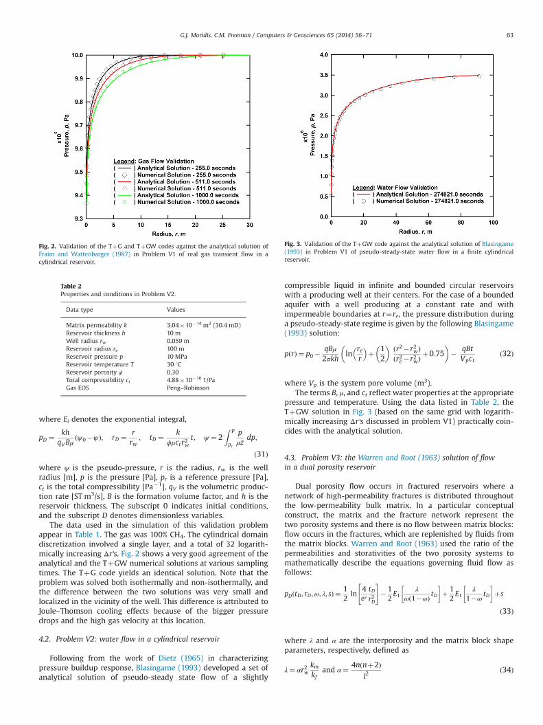
4.1. Problem V1: real gas transient flow in a cylindrical reservoir

Using the concept of pseudo-pressure, Fraim and Wattenbarger(1987) developed a solution to the problem of transient flow in afinite cylindrical real-gas reservoir with a producing vertical wellat its center, described as

pD ¼ 12Ei

r2D4tD

� �ð30Þ

Fnm

Anm x

x

x

D n

D m

Fnm

A nm

V n

V m

n

m

Fig. 1. Space discretization and geometry data in the integral finite differencemethod.

Table 1Properties and conditions in Problem V1.

Data type Values

Matrix permeability k 3.04�10�14 m2 (30.4 mD)Reservoir thickness h 10 mWell radius rw 0.059 mReservoir radius re 100 mReservoir pressure p 10 MPaReservoir temperature T 60 1CReservoir porosity ϕ 0.30Rock compressibility 2�10�10 1/PaGas composition 100% CH4

Gas EOS Peng–Robinson

G.J. Moridis, C.M. Freeman / Computers & Geosciences 65 (2014) 56–7162

where Ei denotes the exponential integral,

pD ¼ khqVBμ

ðψ0�ψÞ; rD ¼ rrw

; tD ¼ kϕμctr2w

t; ψ ¼ 2Z p

pr

pμz

dp;

ð31Þwhere ψ is the pseudo-pressure, r is the radius, rw is the wellradius [m], p is the pressure [Pa], pr is a reference pressure [Pa],ct is the total compressibility [Pa�1], qV is the volumetric produc-tion rate [ST m3/s], B is the formation volume factor, and h is thereservoir thickness. The subscript 0 indicates initial conditions,and the subscript D denotes dimensionless variables.

The data used in the simulation of this validation problemappear in Table 1. The gas was 100% CH4. The cylindrical domaindiscretization involved a single layer, and a total of 32 logarith-mically increasing Δr's. Fig. 2 shows a very good agreement of theanalytical and the TþGW numerical solutions at various samplingtimes. The TþG code yields an identical solution. Note that theproblem was solved both isothermally and non-isothermally, andthe difference between the two solutions was very small andlocalized in the vicinity of the well. This difference is attributed toJoule–Thomson cooling effects because of the bigger pressuredrops and the high gas velocity at this location.

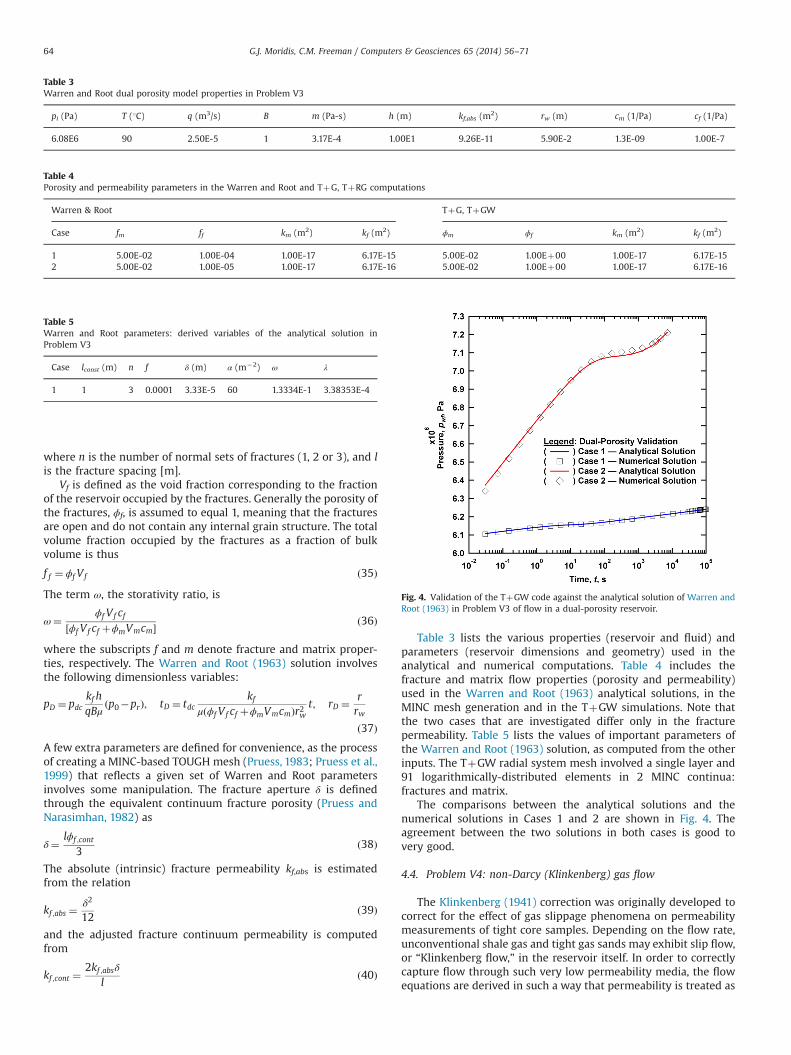
4.2. Problem V2: water flow in a cylindrical reservoir

Following from the work of Dietz (1965) in characterizingpressure buildup response, Blasingame (1993) developed a set ofanalytical solution of pseudo-steady state flow of a slightly

compressible liquid in infinite and bounded circular reservoirswith a producing well at their centers. For the case of a boundedaquifer with a well producing at a constant rate and withimpermeable boundaries at r¼re, the pressure distribution duringa pseudo-steady-state regime is given by the following Blasingame(1993) solution:

pðrÞ ¼ p0�qBμ2πkh

lnrer

� �þ 1

2

� � ðr2�r2wÞðr2e �r2wÞ

þ0:75� �

� qBtVpct

ð32Þ

where Vp is the system pore volume (m3).The terms B, μ, and ct reflect water properties at the appropriate

pressure and temperature. Using the data listed in Table 2, theTþGW solution in Fig. 3 (based on the same grid with logarith-mically increasing Δr's discussed in problem V1) practically coin-cides with the analytical solution.

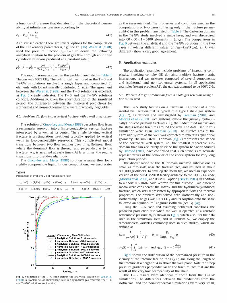
4.3. Problem V3: the Warren and Root (1963) solution of flowin a dual porosity reservoir

Dual porosity flow occurs in fractured reservoirs where anetwork of high-permeability fractures is distributed throughoutthe low-permeability bulk matrix. In a particular conceptualconstruct, the matrix and the fracture network represent thetwo porosity systems and there is no flow between matrix blocks:flow occurs in the fractures, which are replenished by fluids fromthe matrix blocks. Warren and Root (1963) used the ratio of thepermeabilities and storativities of the two porosity systems tomathematically describe the equations governing fluid flow asfollows:

pDðtD; rD;ω; λ; sÞ ¼12ln

4eγ

tDr2D

" #� 1

2E1

λ

ωð1�ωÞ tD�

þ 12E1

λ

1�ωtD

� þs

ð33Þ

where λ and α are the interporosity and the matrix block shapeparameters, respectively, defined as

λ¼ αr2wkmkf

and α¼ 4nðnþ2Þl2

ð34Þ

Fig. 2. Validation of the TþG and TþGW codes against the analytical solution ofFraim and Wattenbarger (1987) in Problem V1 of real gas transient flow in acylindrical reservoir.

Table 2Properties and conditions in Problem V2.

Data type Values

Matrix permeability k 3.04�10�14 m2 (30.4 mD)Reservoir thickness h 10 mWell radius rw 0.059 mReservoir radius re 100 mReservoir pressure p 10 MPaReservoir temperature T 30 1CReservoir porosity ϕ 0.30Total compressibility ct 4.88�10�10 1/PaGas EOS Peng–Robinson

Fig. 3. Validation of the TþGW code against the analytical solution of Blasingame(1993) in Problem V1 of pseudo-steady-state water flow in a finite cylindricalreservoir.

G.J. Moridis, C.M. Freeman / Computers & Geosciences 65 (2014) 56–71 63

where n is the number of normal sets of fractures (1, 2 or 3), and lis the fracture spacing [m].

Vf is defined as the void fraction corresponding to the fractionof the reservoir occupied by the fractures. Generally the porosity ofthe fractures, ϕf, is assumed to equal 1, meaning that the fracturesare open and do not contain any internal grain structure. The totalvolume fraction occupied by the fractures as a fraction of bulkvolume is thus

f f ¼ ϕf V f ð35ÞThe term ω, the storativity ratio, is

ω¼ ϕf V f cf½ϕf V f cf þϕmVmcm�

ð36Þ

where the subscripts f and m denote fracture and matrix proper-ties, respectively. The Warren and Root (1963) solution involvesthe following dimensionless variables:

pD ¼ pdckf hqBμ

ðp0�prÞ; tD ¼ tdckf

μðϕf V f cf þϕmVmcmÞr2wt; rD ¼ r

rwð37Þ

A few extra parameters are defined for convenience, as the processof creating a MINC-based TOUGH mesh (Pruess, 1983; Pruess et al.,1999) that reflects a given set of Warren and Root parametersinvolves some manipulation. The fracture aperture δ is definedthrough the equivalent continuum fracture porosity (Pruess andNarasimhan, 1982) as

δ¼ lϕf ;cont

3ð38Þ

The absolute (intrinsic) fracture permeability kf,abs is estimatedfrom the relation

kf ;abs ¼δ2

12ð39Þ

and the adjusted fracture continuum permeability is computedfrom

kf ;cont ¼2kf ;absδ

lð40Þ

Table 3 lists the various properties (reservoir and fluid) andparameters (reservoir dimensions and geometry) used in theanalytical and numerical computations. Table 4 includes thefracture and matrix flow properties (porosity and permeability)used in the Warren and Root (1963) analytical solutions, in theMINC mesh generation and in the TþGW simulations. Note thatthe two cases that are investigated differ only in the fracturepermeability. Table 5 lists the values of important parameters ofthe Warren and Root (1963) solution, as computed from the otherinputs. The TþGW radial system mesh involved a single layer and91 logarithmically-distributed elements in 2 MINC continua:fractures and matrix.

The comparisons between the analytical solutions and thenumerical solutions in Cases 1 and 2 are shown in Fig. 4. Theagreement between the two solutions in both cases is good tovery good.

4.4. Problem V4: non-Darcy (Klinkenberg) gas flow

The Klinkenberg (1941) correction was originally developed tocorrect for the effect of gas slippage phenomena on permeabilitymeasurements of tight core samples. Depending on the flow rate,unconventional shale gas and tight gas sands may exhibit slip flow,or “Klinkenberg flow,” in the reservoir itself. In order to correctlycapture flow through such very low permeability media, the flowequations are derived in such a way that permeability is treated as

Table 3Warren and Root dual porosity model properties in Problem V3

pi (Pa) T (1C) q (m3/s) B m (Pa-s) h (m) kf,abs (m2) rw (m) cm (1/Pa) cf (1/Pa)

6.08E6 90 2.50E-5 1 3.17E-4 1.00E1 9.26E-11 5.90E-2 1.3E-09 1.00E-7

Table 4Porosity and permeability parameters in the Warren and Root and TþG, TþRG computations

Warren & Root TþG, TþGW

Case fm ff km (m2) kf (m2) ϕm ϕf km (m2) kf (m2)

1 5.00E-02 1.00E-04 1.00E-17 6.17E-15 5.00E-02 1.00Eþ00 1.00E-17 6.17E-152 5.00E-02 1.00E-05 1.00E-17 6.17E-16 5.00E-02 1.00Eþ00 1.00E-17 6.17E-16

Table 5Warren and Root parameters: derived variables of the analytical solution inProblem V3

Case lconst (m) n f δ (m) α (m�2) ω λ

1 1 3 0.0001 3.33E-5 60 1.3334E-1 3.38353E-4

Fig. 4. Validation of the TþGW code against the analytical solution of Warren andRoot (1963) in Problem V3 of flow in a dual-porosity reservoir.

G.J. Moridis, C.M. Freeman / Computers & Geosciences 65 (2014) 56–7164

a function of pressure that deviates from the theoretical perme-ability at infinite gas pressure according to

kg ¼ k1 1þ bp

� �ð41Þ

As discussed earlier, there are several options for the computationof the Klinkenberg parameter b, e.g., see Eq. (16). Wu et al. (1988)used the pressure function pk¼pþb to derive the followinganalytical solution to the problem of gas flow through an infinitecylindrical reservoir produced at a constant rate q:

p2k ðr; tÞ ¼ p2k0�μq

2πk1hctEi � k1pkr

2

4ϕμt

� �ð42Þ

The input parameters used in this problem are listed in Table 6.The gas was 100% CH4. The cylindrical mesh used in the TþG andTþGW simulations involved a single layer and comprised 31elements with logarithmically distributed Δr sizes. The agreementbetween the Wu et al. (1988) and the TþG solutions is excellent,as Fig. 5 clearly indicates. The TþG and the TþGW solutionscoincide. Additionally, given the short duration of the simulatedperiod, the differences between the numerical predictions forisothermal and non-isothermal flow were practically negligible.

4.5. Problem V5: flow into a vertical fracture with a well at its center

The solution of Cinco-Ley and Meng (1988) describes flow froma rectangular reservoir into a finite-conductivity vertical fractureintersected by a well at its center. The single bi-wing verticalfracture is a stimulation treatment typically applied to verticalwells in low-permeability reservoirs. This complicated modeltransitions between two flow regimes over time. Bi-linear flow,where the dominant flow is through and perpendicular to thefracture face, is assumed at early times. At later times, the regimetransitions into pseudo-radial flow.

The Cinco-Ley and Meng (1988) solution assumes flow for aslightly compressible liquid. In our computations, we used water

as the reservoir fluid. The properties and conditions used in thecomputations of two cases (differing only in the fracture perme-ability) in this problem are listed in Table 7. The Cartesian domainin the TþGW study involved a single layer, and was discretizedinto 60�60�1¼3400 elements in (x,y,z). The comparisons inFig. 6 between the analytical and the TþGW solutions in the twocases (involving different values of FCD¼kfbf/(kmxf), as kf wasdifferent) show a very good agreement.

5. Application examples

The application examples include problems of increasing com-plexity, involving complex 3D domains, multiple fracture–matrixinteractions, real gas mixtures composed of several components,and isothermal and non-isothermal systems. In all applicationexamples (except problem A3), the gas was assumed to be 100% CH4.

5.1. Problem A1: gas production from a shale gas reservoir using ahorizontal well

This TþG study focuses on a Cartesian 3D stencil of a hor-izontal well section that is typical of a Type I shale gas system(Fig. 7), as defined and investigated by Freeman (2010) andMoridis et al. (2010). Such systems involve the (usually hydrauli-cally) induced primary fractures (PF), the undisturbed matrix, andthe stress release fractures around the well. The data used in thissimulation were as in Freeman (2010). The surface area of theCartesian system at the well was corrected to reflect its cylindricalgeometry. The simulated 3D domain (Fig. 7) represents the stencilof the horizontal well system, i.e., the smallest repeatable sub-domain that can accurately describe the system behavior. Studiesby Olorode (2011) have confirmed that such stencils are accuraterepresentatives of the behavior of the entire system for very longproduction periods.

The discretization of the 3D domain involved subdivisions assmall as mm-scale near the fracture face, and resulted in about800,000 gridblocks. To develop the mesh file, we used an expandedversion of the MESHMAKER facility available to the TOUGHþ code(Moridis et al., 2008) and its MINC option (Pruess, 1983), in additionto a short FORTRAN code written for this purpose. Two differentmedia were considered: the matrix and the hydraulically-inducedfracture, which was represented by appropriate flow and thermalproperties. The problem was solved both isothermally and non-isothermally. The gas was 100% CH4, and its sorption onto the shalefollowed an equilibrium Langmuir isotherm (see Eq. (4)).

Using the TþG code and assuming isothermal conditions, thepredicted production rate when the well is operated at a constantbottomhole pressure Pw is shown in Fig. 8, which also lists the dataused in the simulation. Here, and in Problem A2, we employ thedimensionless variables commonly used in such studies, which aredefined as

tD ¼ kφμctx2f

1½1þVL�

t; qD ¼ Bμkhðpi�pwf Þ

q ð40Þ

qDiðtÞ ¼1t

Z t

0qDðτÞdτ; and qDidðtÞ ¼ �t

dqDidt

ð41Þ

Fig. 9 shows the distribution of the normalized pressure in thevicinity of the fracture face on the (x,y) plane along the length ofthe fracture at a height of 4 m above the well plane. Note the steeppressure gradients perpendicular to the fracture face that are theresult of the very low permeability of the shale.

The TþG results were identical to those from the TþGWsimulations. The differences between the predictions from theisothermal and the non-isothermal simulations were very small,

Table 6Parameters in Problem V4 of Klinkenberg flow.

k1 (m2) b (1/Pa) pi (Pa) μ (Pa-s) ϕ h (m) q (m3/s) ct (1/Pa) z

3.0E-14 73830.6 1.00E7 1.44E-5 0.3 10 1.54E-2 1.07E-7 0.89

Fig. 5. Validation of the TþG code against the analytical solution of Wu et al.(1988) in Problem V4 of Klinkenberg flow in a cylindrical gas reservoir. The TþGand TþGW solutions are identical.

G.J. Moridis, C.M. Freeman / Computers & Geosciences 65 (2014) 56–71 65

became perceptible at late times, and cannot register as differenton the log–log plots (such as the one in Fig. 8) typically used insuch studies.

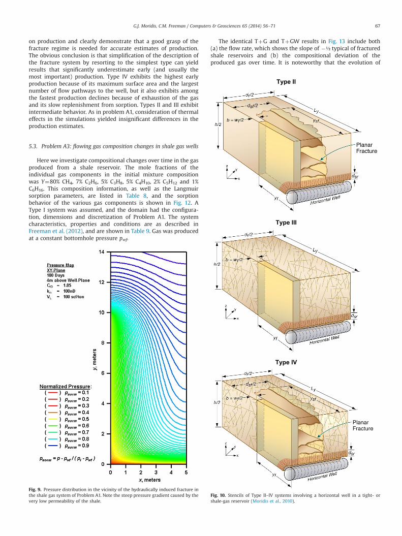
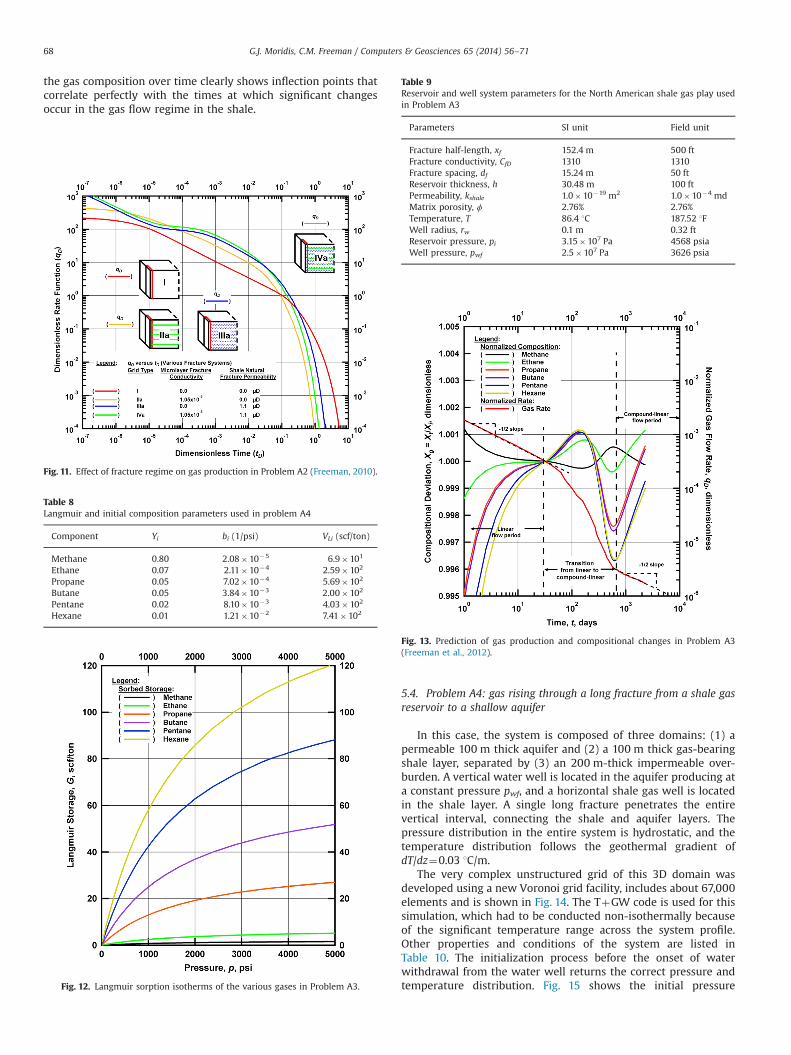
5.2. Problem A2: gas production from a shale gas reservoir with acomplex fracture system using a horizontal well

Problem A2 is a sensitivity analysis study that aims to determinethe effects of more complex fracture regimes. These are representedby Types II, III and IV (Fig. 10), which include secondary planarfractures (generally perpendicular to the primary fractures), naturalfractures, and all types of fractures, respectively. Type IV is the mostcomplex system to describe, simulate and analyze. The data in thesesimulations were as in Freeman (2010). These complex systems

involved three individual subdomains, each with appropriate prop-erties: the matrix, the main (hydraulically-induced) fracture, andthe secondary planar fractures. The natural fractures were describedby a dual-porosity model using the MINC concept (Pruess, 1983) todescribe a dual-permeability (as opposed to a dual porosity) modelof fracture–matrix interactions.

With the exception of the properties of the various fracturesystems, all properties and conditions of the reservoir and of thefluid remained as in Problem A1. The discretization of the 3Ddomains included subdivisions as small as mm-scale near thefracture face, and resulted in about a number of gridblocks thatvaried from about 850,000 elements in the Type II system to about1,200,000 in the Type IV system. The TþG and TþGW simulationswere conducted in both isothermal and non-isothermal modes.

The TþG and TþGW results coincided, and are shown in Fig. 11(which includes the Type I predictions for reference). The fourdomain types exhibit very different production patterns andperformance. The significant discrepancies of the various produc-tion estimates indicate the importance of the additional fractures

Table 7Properties and conditions in Problem V5.

Case pi (kPa) km (mm2) kf (mm2) h (m) q (m3/d) B μ (Pa s) ϕm ct (1/Pa) xf (m) FcD bf (m)

1 1.0E5 3.3E-3 3.0E3 10 172.8 1 4.91E-4 0.3 3.37E-10 20 103 0.0222 1.0E5 3.3E-4 3.0E3 10 172.8 1 4.91E-4 0.3 3.37E-10 20 104 0.022

Fig. 6. Validation of the TþGW code against the analytical solutions of Cinco-Ley and Meng (1988) in Problem V5 of flow into a vertical fracture intersected by a vertical wellat its center. Case 1: FCD¼103; Case 2: FCD¼104.

Fig. 7. Stencil of a Type I system involving a horizontal well in a tight- or shale-gasreservoir (Moridis et al., 2010).

Fig. 8. Prediction of gas production in Problem A1 (Freeman, 2010).

G.J. Moridis, C.M. Freeman / Computers & Geosciences 65 (2014) 56–7166

on production and clearly demonstrate that a good grasp of thefracture regime is needed for accurate estimates of production.The obvious conclusion is that simplification of the description ofthe fracture system by resorting to the simplest type can yieldresults that significantly underestimate early (and usually themost important) production. Type IV exhibits the highest earlyproduction because of its maximum surface area and the largestnumber of flow pathways to the well, but it also exhibits amongthe fastest production declines because of exhaustion of the gasand its slow replenishment from sorption. Types II and III exhibitintermediate behavior. As in problem A1, consideration of thermaleffects in the simulations yielded insignificant differences in theproduction estimates.

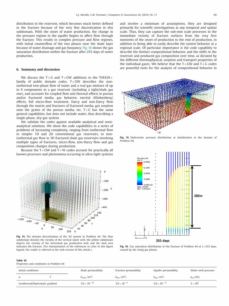
5.3. Problem A3: flowing gas composition changes in shale gas wells

Here we investigate compositional changes over time in the gasproduced from a shale reservoir. The mole fractions of theindividual gas components in the initial mixture compositionwas Y¼80% CH4, 7% C2H6, 5% C3H8, 5% C4H10, 2% C5H12 and 1%C6H16. This composition information, as well as the Langmuirsorption parameters, are listed in Table 8, and the sorptionbehavior of the various gas components is shown in Fig. 12. AType I system was assumed, and the domain had the configura-tion, dimensions and discretization of Problem A1. The systemcharacteristics, properties and conditions are as described inFreeman et al. (2012), and are shown in Table 9. Gas was producedat a constant bottomhole pressure pwf.

The identical TþG and TþGW results in Fig. 13 include both(a) the flow rate, which shows the slope of �½ typical of fracturedshale reservoirs and (b) the compositional deviation of theproduced gas over time. It is noteworthy that the evolution of

Fig. 9. Pressure distribution in the vicinity of the hydraulically induced fracture inthe shale gas system of Problem A1. Note the steep pressure gradient caused by thevery low permeability of the shale.

Type II

Type III

Type IV

Fig. 10. Stencils of Type II–IV systems involving a horizontal well in a tight- orshale-gas reservoir (Moridis et al., 2010).

G.J. Moridis, C.M. Freeman / Computers & Geosciences 65 (2014) 56–71 67

the gas composition over time clearly shows inflection points thatcorrelate perfectly with the times at which significant changesoccur in the gas flow regime in the shale.

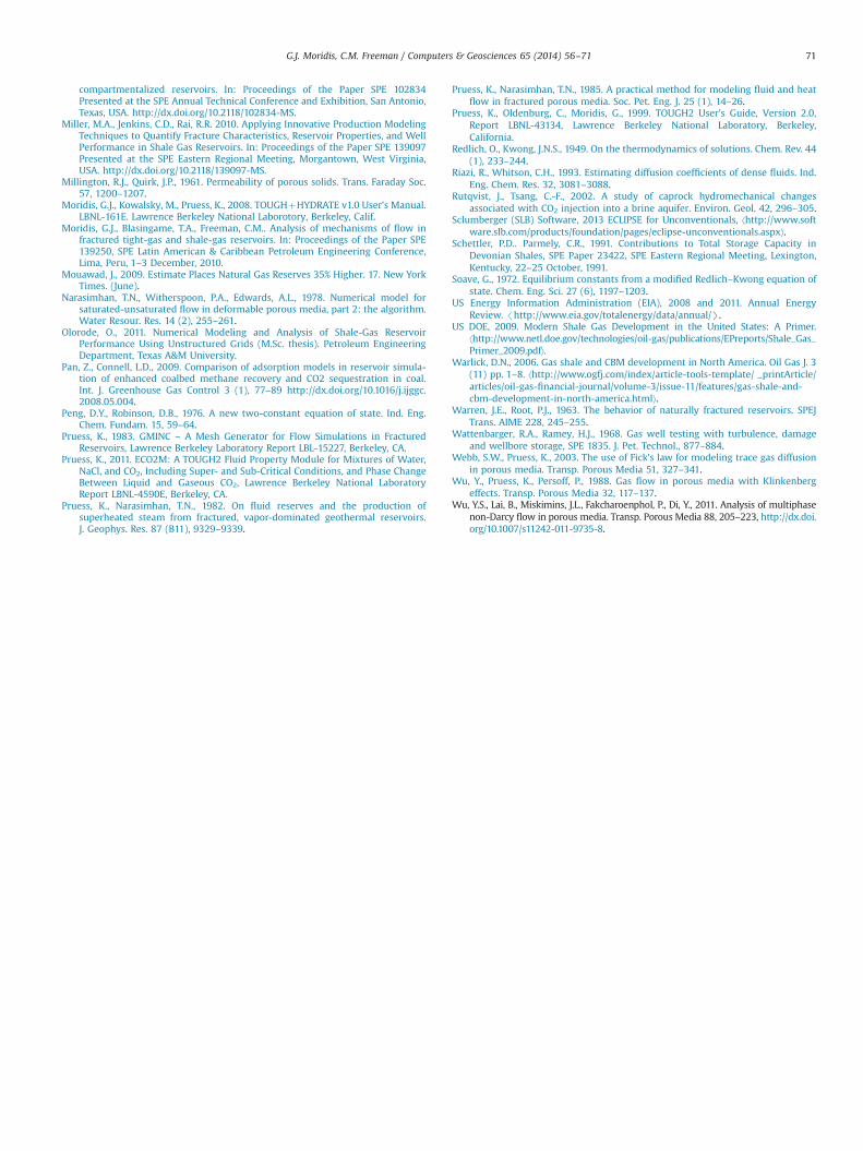
5.4. Problem A4: gas rising through a long fracture from a shale gasreservoir to a shallow aquifer

In this case, the system is composed of three domains: (1) apermeable 100 m thick aquifer and (2) a 100 m thick gas-bearingshale layer, separated by (3) an 200 m-thick impermeable over-burden. A vertical water well is located in the aquifer producing ata constant pressure pwf, and a horizontal shale gas well is locatedin the shale layer. A single long fracture penetrates the entirevertical interval, connecting the shale and aquifer layers. Thepressure distribution in the entire system is hydrostatic, and thetemperature distribution follows the geothermal gradient ofdT/dz¼0.03 1C/m.

The very complex unstructured grid of this 3D domain wasdeveloped using a new Voronoi grid facility, includes about 67,000elements and is shown in Fig. 14. The TþGW code is used for thissimulation, which had to be conducted non-isothermally becauseof the significant temperature range across the system profile.Other properties and conditions of the system are listed inTable 10. The initialization process before the onset of waterwithdrawal from the water well returns the correct pressure andtemperature distribution. Fig. 15 shows the initial pressure

Fig. 11. Effect of fracture regime on gas production in Problem A2 (Freeman, 2010).

Table 8Langmuir and initial composition parameters used in problem A4

Component Yi bi (1/psi) VLi (scf/ton)

Methane 0.80 2.08�10�5 6.9�101

Ethane 0.07 2.11�10�4 2.59�102

Propane 0.05 7.02�10�4 5.69�102

Butane 0.05 3.84�10�3 2.00�102

Pentane 0.02 8.10�10�3 4.03�102

Hexane 0.01 1.21�10�2 7.41�102

Fig. 12. Langmuir sorption isotherms of the various gases in Problem A3.

Table 9Reservoir and well system parameters for the North American shale gas play usedin Problem A3

Parameters SI unit Field unit

Fracture half-length, xf 152.4 m 500 ftFracture conductivity, CfD 1310 1310Fracture spacing, df 15.24 m 50 ftReservoir thickness, h 30.48 m 100 ftPermeability, kshale 1.0�10�19 m2 1.0�10�4 mdMatrix porosity, ϕ 2.76% 2.76%Temperature, T 86.4 1C 187.52 1FWell radius, rw 0.1 m 0.32 ftReservoir pressure, pi 3.15�107 Pa 4568 psiaWell pressure, pwf 2.5�107 Pa 3626 psia

Fig. 13. Prediction of gas production and compositional changes in Problem A3(Freeman et al., 2012).

G.J. Moridis, C.M. Freeman / Computers & Geosciences 65 (2014) 56–7168

distribution in the reservoir, which becomes much better definedin the fracture because of the very fine discretization in thissubdomain. With the onset of water production, the change inthe pressure regime in the aquifer begins to affect flow throughthe fracture. This results in complex pressure and flow regimes,with initial counterflow of the two phases near the shale layerbecause of water drainage and gas buoyancy. Fig. 16 shows the gassaturation distribution within the fracture after 255 days of waterproduction.

6. Summary and discussion

We discuss the TþG and TþGW additions to the TOUGHþfamily of public domain codes. TþGW describes the non-isothermal two-phase flow of water and a real gas mixture of upto 9 components in a gas reservoir (including a tight/shale gasone), and accounts for coupled flow and thermal effects in porousand/or fractured media, gas behavior, inertial (Klinkenberg)effects, full micro-flow treatment, Darcy and non-Darcy flowthrough the matrix and fractures of fractured media, gas sorptiononto the grains of the porous media, etc. TþG has the samegeneral capabilities, but does not include water, thus describing asingle-phase, dry-gas system.

We validate the codes against available analytical and semi-analytical solutions. We show the code capabilities in a series ofproblems of increasing complexity, ranging from isothermal flowin simpler 1D and 2D conventional gas reservoirs, to non-isothermal gas flow in 3D fractured shale gas reservoirs involvingmultiple types of fractures, micro-flow, non-Darcy flow and gascomposition changes during production.

Because the TþGW and TþW codes account for practically allknown processes and phenomena occurring in ultra-tight systems

and involve a minimum of assumptions, they are designedprimarily for scientific investigations at any temporal and spatialscale. Thus, they can capture the sub-mm scale processes in theimmediate vicinity of fracture surfaces from the very firstmoments of the onset of production to the end of production, inaddition to being able to easily describe the system behavior at aregional scale. Of particular importance is the code capability todescribe the distinct compositional behavior, and the shifts in thereservoir and produced gas composition over time, as dictated bythe different thermophysical, sorption and transport properties ofthe individual gases. We believe that the TþGW and TþG codesare powerful tools for the analysis of compositional behavior in

Fig. 14. The domain discretization of the 3D system in Problem A4. The bluesubdomain denotes the vicinity of the vertical water well, the yellow subdomaindepicts the vicinity of the horizontal gas production well, and the dark areaindicates the fracture. (For interpretation of the references to color in this figurelegend, the reader is referred to the web version of this article.)

Table 10Properties and conditions in Problem A4

Initial conditions Shale permeability Fracture permeability Aquifer permeability Water well pressure

p T kshale (m2) kfrac (m2) kaqu (m2) pwf (Pa)

Geothermal/hydrostatic gradient 3.0�10�19 3.0�10�9 3.0�10�13 5�106

Fig. 15. Hydrostatic pressure distribution at initialization in the domain ofProblem A4.

Fig. 16. Gas saturation distribution in the fracture of Problem A4 at t¼255 days,caused by the rising gas plume.

G.J. Moridis, C.M. Freeman / Computers & Geosciences 65 (2014) 56–71 69

gas-rich reservoirs and particularly ultra-tight ones, for testinghypotheses and gaining insights in the evaluation of dominantflow and transport mechanisms, for parameter estimation throughhistory-matching (optimization) processes, for reserve estimationand for production forecasting.

In addition to its benefits to the analysis of hydrocarbon gasreservoirs, it is important to indicate that the TþGW code is fullyapplicable to a wide variety of other problems, including environ-mental studies on the impact of escaping gaseous hydrocarbonsinto overlying potable water aquifers (see problem A4), the studyof the geological storage of greenhouse gas mixtures, and theinvestigation of the performance of geothermal reservoirs withmulti-component non-condensable gas mixtures. Although mostissues were not included in this study, they are to be included infuture publications on the range of applications of TþGW.

There are several ideas about inclusion of additional optionsand capabilities into the TþGW. Expansion of the library of non-condensable gases (and the corresponding number of equations) isa relatively simple endeavor. Accounting for brines (by adding amass balance equation for salts) is currently the highest priority.The addition of capabilities to handle condensable hydrocarbongases is also a high-priority, as this would allow the study ofproduction of retrograde gases (condensates) that are of higheconomic importance.

Acknowledgments

The research described in this article has been funded by theU.S. Environmental Protection Agency through Interagency Agree-ment (DW-89-92235901-C) to the Lawrence Berkeley NationalLaboratory, and by the Research Partnership to Secure Energy forAmerica (RPSEA) – (Contract no. 08122-45) through the Ultra-Deepwater and Unconventional Natural Gas and Other PetroleumResources Research and Development Program as authorized bythe US Energy Policy Act (EPAct) of 2005. The views expressed inthis article are those of the author(s) and do not necessarily reflectthe views or policies of the EPA.

References

Americal Petroleum Institute (API), 2013. Policy Issues: Facts about Shale Gas.⟨http://www.api.org/policy-and-issues/policy-items/exploration/facts_about_shale_gas⟩.

Anderson, D.M., Nobakht, M., Moghadam, S., et al., 2010. Analysis of productiondata from fractured shale gas wells. In: Proceedings of the Paper SPE 131787Presented at the SPE Unconventional Gas Conference, Pittsburgh, Pennsylvania,USA. http://dx.doi.org/10.2118/131787-MS.

Barree, R.D., Conway, M.W., 2007. Multiphase non-Darcy flow in proppant packs,Paper SPE 109561. In: Proceedings of the Annual Technical Conference andExhibition, Anaheim, CA, 11–14 November, 2007.

Bello, R.O., Wattenbarger, R.A., 2008. Rate transient analysis in naturally fracturedshale gas reservoirs. In: Proceedings of the Paper SPE 114591 Presented at theCIPC/SPE Gas Technology Symposium 2008 Joint Conference, Calgary, Alberta,Canada. http://dx.doi.org/10.2118/114591-MS.

Bird, R.B., Stewart, W.E., Lightfoot, E.N., 2007. Transport Phenomena. John Wiley &Sons, Inc., New York.

Blasingame, 1993. T.A., Semi-analytical solutions for a bounded circular reservoir –no flow and constant pressure outer boundary conditions: unfractured wellcase. Paper SPE 25479, SPE Production Operations Symposium, Oklahoma City,Oklahoma, 21–23 March, 1993.

Blasingame, T.A., Poe Jr., B.D. 1993. Semianalytic solutions for a well with a singlefinite-conductivity vertical fracture. In: Proceedings of the Paper SPE 26424Presented at the SPE Annual Technical Conference and Exhibition, Houston,Texas, USA. http://dx.doi.org/10.2118/26424-MS.

Computer Modeling Group (CMG), 2013. GEM General Release (GEM 2013.10),⟨http://www.cmgl.ca/software/soft-gem⟩.

Chung, T.H., Ajlan, M., Lee, L.L., Starling, K.E., 1988. Generalized multiparametercorrelation for nonpolar and polar fluid transport properties. Ind. Eng. Chem.Res. 27 (4), 671–679, http://dx.doi.org/10.1021/ie00076a024.

Cinco-Ley, H., Meng, H.-Z., 1988. Pressure transient analysis of wells with finiteconductivity vertical fractures in double porosity reservoirs. In: Proceedings ofthe Paper SPE 18172-MS Presented at the SPE Annual Technical Conference and

Exhibition, Houston, Texas, 2–5 October, 1988. http://dx.doi.org/10.2118/18172-MS.

Cinco-Ley, H., Samaniego, F., Dominguez, N., 1978. Transient pressure behavior for awell with a finite-conductivity vertical fracture. SPE J. 18 (4), 253–264. (SPE6014-PA)http://dx.doi.org/10.2118/6014-PA.

Cipolla, C.L., Lolon, E., Erdle, J., et al., 2009. Modeling well performance in shale-gasreservoirs. In: Proceedings of the Paper SPE 125532 Presented at the SPE/EAGEReservoir Characterization and Simulation Conference, Abu Dhabi, UAE. http://dx.doi.org/10.2118/125532-MS.

Civan, F., 2008. Effective correlation of apparent gas permeability in tight porousmedia. Transp. Porous Media 83, 375–384.

Clarkson, C.R., Bustin, R.M., 1999. Binary gas adsorption/desorption isotherms:effect of moister and coal composition upon carbon dioxide selectivity overmethane. Int. J. Coal Geol. 42, 241–271.

Dietz, D.N., 1965. Determination of average reservoir pressure from build-upsurveys. J. Pet. Technol., 955–959.

Doronin, G.G., Larkin, N.A., 2004. On dusty gas model governed by the Kuramoto–Sivashinsky equation. Comput. Appl. Math. 23 (1), 67–80.

Edwards, A.L., 1972. TRUMP: A Computer Program for Transient and Steady StateTemperature Distributions in Multidimensional Systems. National TechnicalInformation Service, National Bureau of Standards, Springfield, VA.

Finsterle, S., 2001. Implementation of the Forchheimer Equation in iTOUGH2,Project Report. Lawrence Berkeley National Laboratory, Berkeley, California.

Florence, F.A., Rushing, J.A., Newsham, K.E., Blasingame, T.A., 2007. Improvedpermeability prediction relations for low-permeability sands. SPE paper107954 presented at the SPE Rocky Mountain Oil and Gas TechnologySymposium. 16–18 April Denver, Colorado.

Forchheimer, P., 1901. Wasserbewewegung durch Boden. Zeit. Ver. Dtsch. Ing. 45,1781.

Fraim, M.L., Wattenbarger, R.A., 1987. Gas reservoir decline curve analysis usingtype curves with real gas pseudopressure and pseudotime. SPEFE, 671–682.

Freeman, C.M., 2010 Study of Flow Regimes in Multiply-Fractured Horizontal Wellsin Tight Gas and shale Gas Reservoir Systems (M.Sc. thesis). PetroleumEngineering Department, Texas A&M University.

Freeman, C.M., Moridis, G.J., Ilk, D. et al., 2009. A numerical study of performancefor tight gas and shale gas reservoir systems. In: Proceedings of the Paper SPE124961 Presented at the SPE Annual Technical Conference and Exhibition,New Orleans, Louisiana, USA. http://dx.doi.org/10.2118/124961-MS.

Freeman, C.M., Moridis, G.J., Blasingame, T.A., 2011. A numerical study of microscaleflow behavior in tight gas and shale gas reservoir systems. Transp. PorousMedia 90 (1), 253–268, http://dx.doi.org/10.1007/ s11242-011-9761-6.

Freeman, C.M., G.J. Moridis, E. Michael, T.A. Blasingame, 2012. Measurement, modeling,and diagnostics of flowing gas composition changes in shale gas wells, Paper SPE153391, In: Proceedings of the SPE Latin American and Caribbean PetroleumEngineering Conference, Mexico City, Mexico, 16–18 April, 2012.

Freeman, C.M., Moridis, G.J., Ilk, D., Blasingame, T.A., 2013. A numerical study ofperformance for tight gas and shale gas reservoir systems. J. Pet. Sci. Eng. 108,22–39 http://dx.doi.org/10.1016/j.petrol.%202013.05.007.

Fuller, E.N., Schettler, P.D., Giddings, J.C., 1966. A new method for prediction ofbinary gas-phase diffusion coefficients. Ind. Eng. Chem. 58, 19–27.

Gao, C., Lee, J.W., Spivey, J.P., Semmelbeck, M.E. Modeling multilayer gas reservoirsincluding sorption effects, SPE Paper 29173, In: Proceedings of the SPE EasternRegional Conference & Exhibition, Charleston, West Virginia, 8–10 November, 1994.

Gringarten, A.C., 1971. Unsteady-State Pressure Distributions Created by a Well witha Single Horizontal Fracture, Partial Penetration, or Restricted Entry (Ph.D.dissertation), Stanford University, Stanford, California, USA.

Gringarten, A.C., Henry, J., Ramey, J., Raghavan, R., 1974. Unsteady-state pressuredistributions created by a well with a single infinite-conductivity verticalfracture. SPE J. 14 (4), http://dx.doi.org/10.2118/4051-PA.

Houze, O., Tauzin, E., Artus, V., et al., 2010. The Analysis of Dynamic Data in Shale GasReservoirs – Part 1. Company report, Kappa Engineering, Houston, Texas, USA.

International Formulation Committee (IFC), 1967. A Formulation of the Thermo-dynamic Properties of Ordinary Water Substance, IFC Secretariat, Düsseldorf,Germany.

Jayakumar, R., Sahai, V., Boulis, A., 2011. A better understanding of finite elementsimulation for shale gas reservoirs through a series of different case histories.In: Proceedings of the Paper SPE 142464 Presented at the SPE Middle EastUnconventional Gas Conference and Exhibition, Muscat, Oman. http://dx.doi.org/10.2118/142464-MS.

Jones, S.C., 1972. A rapid accurate unsteady-state Klinkenberg parameter. SPE J.,383–397.

Karniadakis, G.E., Beskok, A., 2001. Microflows: Fundamentals and Simulation.Springer, Berlin.

Katz, D.L., et al., 1959. Handbook of Natural Gas Engineering. McGraw-Hill, New York.Kim, J., Moridis, G.J., 2013. Development of the TþM coupled flow-geomechanical

simulator to describe fracture propagation and coupled flow-thermal-geomechanical processes in tight/shale gas systems. Comput. Geosci. 60,184–198, http://dx.doi.org/10.1016/j.cageo.2013.04.023.

Klinkenberg, L.J., 1941 The Permeability of Porous Media to Liquid and Gases,Proceedings, API Drilling and Production Practice, pp. 200–213.

Mattar, L., 2008. Production analysis and forecasting of shale gas reservoirs: casehistory-based approach. In: Proceedings of the Paper SPE 119897 Presented atthe SPE Shale Gas Production Conference, Fort Worth, Texas, USA. http://dx.doi.org/10.2118/119897-MS.

Medeiros, F., Ozkan, E., Kazemi, H., 2006. A semianalytical, pressure-transientmodel for horizontal and multilateral wells in composite, layered, and

G.J. Moridis, C.M. Freeman / Computers & Geosciences 65 (2014) 56–7170

compartmentalized reservoirs. In: Proceedings of the Paper SPE 102834Presented at the SPE Annual Technical Conference and Exhibition, San Antonio,Texas, USA. http://dx.doi.org/10.2118/102834-MS.

Miller, M.A., Jenkins, C.D., Rai, R.R. 2010. Applying Innovative Production ModelingTechniques to Quantify Fracture Characteristics, Reservoir Properties, and WellPerformance in Shale Gas Reservoirs. In: Proceedings of the Paper SPE 139097Presented at the SPE Eastern Regional Meeting, Morgantown, West Virginia,USA. http://dx.doi.org/10.2118/139097-MS.

Millington, R.J., Quirk, J.P., 1961. Permeability of porous solids. Trans. Faraday Soc.57, 1200–1207.

Moridis, G.J., Kowalsky, M., Pruess, K., 2008. TOUGHþHYDRATE v1.0 User's Manual.LBNL-161E. Lawrence Berkeley National Laborotory, Berkeley, Calif.

Moridis, G.J., Blasingame, T.A., Freeman, C.M.. Analysis of mechanisms of flow infractured tight-gas and shale-gas reservoirs. In: Proceedings of the Paper SPE139250, SPE Latin American & Caribbean Petroleum Engineering Conference,Lima, Peru, 1–3 December, 2010.

Mouawad, J., 2009. Estimate Places Natural Gas Reserves 35% Higher. 17. New YorkTimes. (June).

Narasimhan, T.N., Witherspoon, P.A., Edwards, A.L., 1978. Numerical model forsaturated-unsaturated flow in deformable porous media, part 2: the algorithm.Water Resour. Res. 14 (2), 255–261.

Olorode, O., 2011. Numerical Modeling and Analysis of Shale-Gas ReservoirPerformance Using Unstructured Grids (M.Sc. thesis). Petroleum EngineeringDepartment, Texas A&M University.

Pan, Z., Connell, L.D., 2009. Comparison of adsorption models in reservoir simula-tion of enhanced coalbed methane recovery and CO2 sequestration in coal.Int. J. Greenhouse Gas Control 3 (1), 77–89 http://dx.doi.org/10.1016/j.ijggc.2008.05.004.

Peng, D.Y., Robinson, D.B., 1976. A new two-constant equation of state. Ind. Eng.Chem. Fundam. 15, 59–64.

Pruess, K., 1983. GMINC – A Mesh Generator for Flow Simulations in FracturedReservoirs, Lawrence Berkeley Laboratory Report LBL-15227, Berkeley, CA.

Pruess, K., 2011. ECO2M: A TOUGH2 Fluid Property Module for Mixtures of Water,NaCl, and CO2, Including Super- and Sub-Critical Conditions, and Phase ChangeBetween Liquid and Gaseous CO2, Lawrence Berkeley National LaboratoryReport LBNL-4590E, Berkeley, CA.

Pruess, K., Narasimhan, T.N., 1982. On fluid reserves and the production ofsuperheated steam from fractured, vapor-dominated geothermal reservoirs.J. Geophys. Res. 87 (B11), 9329–9339.

Pruess, K., Narasimhan, T.N., 1985. A practical method for modeling fluid and heatflow in fractured porous media. Soc. Pet. Eng. J. 25 (1), 14–26.

Pruess, K., Oldenburg, C., Moridis, G., 1999. TOUGH2 User's Guide, Version 2.0,Report LBNL-43134, Lawrence Berkeley National Laboratory, Berkeley,California.

Redlich, O., Kwong, J.N.S., 1949. On the thermodynamics of solutions. Chem. Rev. 44(1), 233–244.

Riazi, R., Whitson, C.H., 1993. Estimating diffusion coefficients of dense fluids. Ind.Eng. Chem. Res. 32, 3081–3088.

Rutqvist, J., Tsang, C.-F., 2002. A study of caprock hydromechanical changesassociated with CO2 injection into a brine aquifer. Environ. Geol. 42, 296–305.

Sclumberger (SLB) Software, 2013 ECLIPSE for Unconventionals, ⟨http://www.software.slb.com/products/foundation/pages/eclipse-unconventionals.aspx⟩.

Schettler, P.D.. Parmely, C.R., 1991. Contributions to Total Storage Capacity inDevonian Shales, SPE Paper 23422, SPE Eastern Regional Meeting, Lexington,Kentucky, 22–25 October, 1991.

Soave, G., 1972. Equilibrium constants from a modified Redlich–Kwong equation ofstate. Chem. Eng. Sci. 27 (6), 1197–1203.

US Energy Information Administration (EIA), 2008 and 2011. Annual EnergyReview. /http://www.eia.gov/totalenergy/data/annual/S.

US DOE, 2009. Modern Shale Gas Development in the United States: A Primer.⟨http://www.netl.doe.gov/technologies/oil-gas/publications/EPreports/Shale_Gas_Primer_2009.pdf⟩.

Warlick, D.N., 2006. Gas shale and CBM development in North America. Oil Gas J. 3(11) pp. 1–8. ⟨http://www.ogfj.com/index/article-tools-template/ _printArticle/articles/oil-gas-financial-journal/volume-3/issue-11/features/gas-shale-and-cbm-development-in-north-america.html⟩.

Warren, J.E., Root, P.J., 1963. The behavior of naturally fractured reservoirs. SPEJTrans. AIME 228, 245–255.

Wattenbarger, R.A., Ramey, H.J., 1968. Gas well testing with turbulence, damageand wellbore storage, SPE 1835. J. Pet. Technol., 877–884.

Webb, S.W., Pruess, K., 2003. The use of Fick's law for modeling trace gas diffusionin porous media. Transp. Porous Media 51, 327–341.

Wu, Y., Pruess, K., Persoff, P., 1988. Gas flow in porous media with Klinkenbergeffects. Transp. Porous Media 32, 117–137.

Wu, Y.S., Lai, B., Miskimins, J.L., Fakcharoenphol, P., Di, Y., 2011. Analysis of multiphasenon-Darcy flow in porous media. Transp. Porous Media 88, 205–223, http://dx.doi.org/10.1007/s11242-011-9735-8.

G.J. Moridis, C.M. Freeman / Computers & Geosciences 65 (2014) 56–71 71