The Relationship between consumer confidence and the stock market in the European Union Master Thesis, Quantitative Finance N.L. Kloet* Supervisor: Prof. Dr. D.J.C. van Dijk Co-reader: Dr. W.W. Tham August, 2013 *Erasmus University Rotterdam, Erasmus School of Economics, MSc Econometrics and Management Science, Quantitative Finance, Student number: 297498 Abstract This thesis uses the consumer confidence index (CCI) and the headline stock indices of 11 European countries to study the relationship between the CCI and the stock market. The co-movement between the CCI and the stock market are examined by using a VAR model, testing for Granger causality and estimating the dependence structure by using copula models. I find that, the stock market has a significant influence on the consumer confidence. Although there is a slight change in correlation through time and in different stages of the economy, this influence does not significantly change.
Transcript
The Relationship between consumer confidence and the stock
market in the European Union
Master Thesis, Quantitative Finance
N.L. Kloet*
Supervisor: Prof. Dr. D.J.C. van Dijk
Co-reader: Dr. W.W. Tham
August, 2013
*Erasmus University Rotterdam, Erasmus School of Economics, MSc Econometrics and Management Science,
Quantitative Finance, Student number: 297498
Abstract
This thesis uses the consumer confidence index (CCI) and the headline stock indices of 11 European
countries to study the relationship between the CCI and the stock market. The co-movement
between the CCI and the stock market are examined by using a VAR model, testing for Granger
causality and estimating the dependence structure by using copula models. I find that, the stock
market has a significant influence on the consumer confidence. Although there is a slight change in
correlation through time and in different stages of the economy, this influence does not significantly
MIB (Italy), AEX (Netherlands), PSI20 (Portugal), IBEX35 (Spain), and FTSE100 (UK). These ‘headline’
stock indices are used because they are most mentioned in news reports. They are extracted from
the database Datastream were they are presented on a daily basis. Because there is not a clear cut
when the CCI data is measured I defined the monthly stock market value as the average of the stock
index of all the data points in that month. This may give some spurious correlation or causality
estimates due to asynchronous observed data. The sample period for Germany, Ireland3, Italy,
Netherlands, and the UK runs from January 1985 to June 2012. The sample periods for the other
countries runs as follows: Belgium (1990M01-2012M06), Denmark (1989M12-2012M06), France
(1987M07-2012M06), Greece (1997M09-2012M06), Portugal (1992M12-2012M06) and Spain
(1987M01-2012M06).
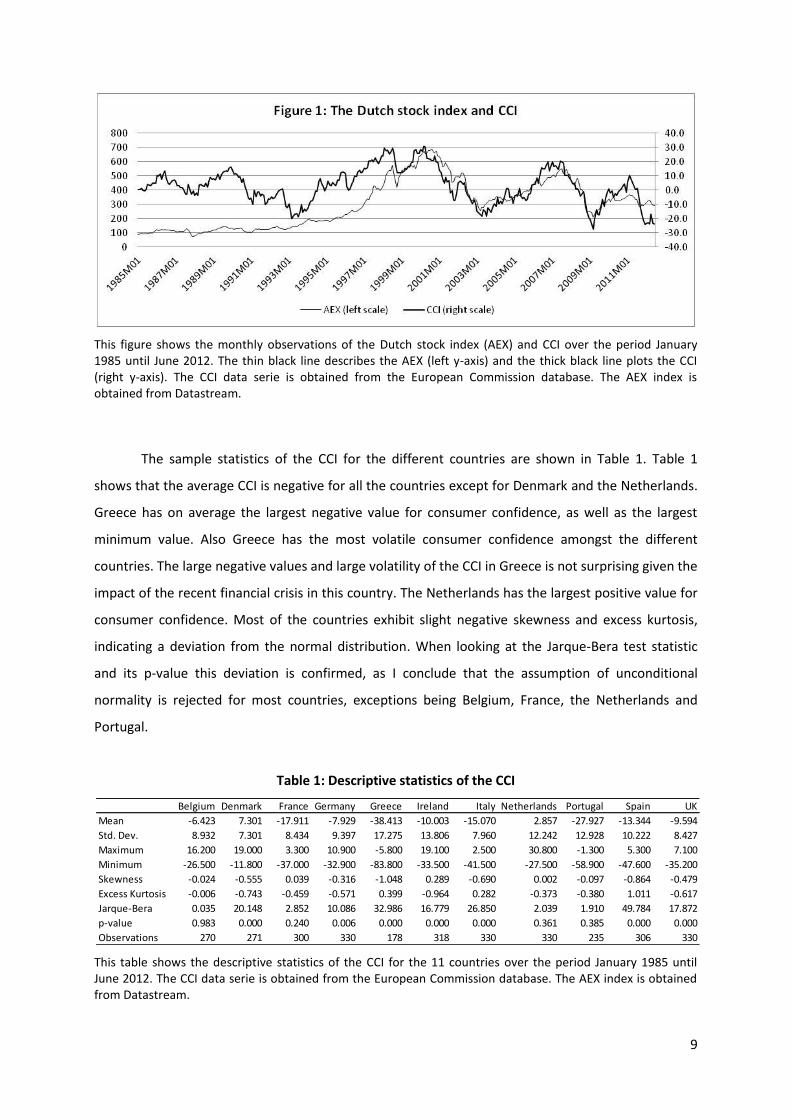
Figure 1 shows the CCI of the Netherlands and the Dutch stock index, the AEX. Here is
suggested that the consumer confidence and the stock market of the Netherlands are related to each
other. As well as that after a certain period this relationship is stronger than before.
1The results are seasonally adjusted by Dainties method. Dainties method is based on the use of filters. A
Dainties filter can be defined as a tool that provides a seasonal component. By subtracting this seasonal
component from the original observation you obtain the seasonal adjusted observation.
2 The ISEQ is the only Overall Index I take into account. This is due to the fact that the ‘headline’ index data,
ISEQ 20, is available from 31 December 2004. This would result in a relatively short sample period. 3 For Ireland the CCI is not measured over the period May 2008 until April 2009.
9
This figure shows the monthly observations of the Dutch stock index (AEX) and CCI over the period January 1985 until June 2012. The thin black line describes the AEX (left y-axis) and the thick black line plots the CCI (right y-axis). The CCI data serie is obtained from the European Commission database. The AEX index is obtained from Datastream.
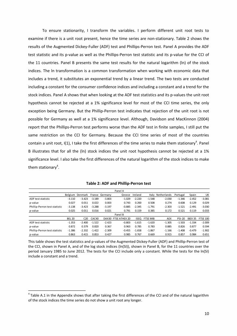
The sample statistics of the CCI for the different countries are shown in Table 1. Table 1
shows that the average CCI is negative for all the countries except for Denmark and the Netherlands.
Greece has on average the largest negative value for consumer confidence, as well as the largest
minimum value. Also Greece has the most volatile consumer confidence amongst the different
countries. The large negative values and large volatility of the CCI in Greece is not surprising given the
impact of the recent financial crisis in this country. The Netherlands has the largest positive value for
consumer confidence. Most of the countries exhibit slight negative skewness and excess kurtosis,
indicating a deviation from the normal distribution. When looking at the Jarque-Bera test statistic
and its p-value this deviation is confirmed, as I conclude that the assumption of unconditional
normality is rejected for most countries, exceptions being Belgium, France, the Netherlands and
Portugal.
Table 1: Descriptive statistics of the CCI
This table shows the descriptive statistics of the CCI for the 11 countries over the period January 1985 until June 2012. The CCI data serie is obtained from the European Commission database. The AEX index is obtained from Datastream.
Belgium Denmark France Germany Greece Ireland Italy Netherlands Portugal Spain UK
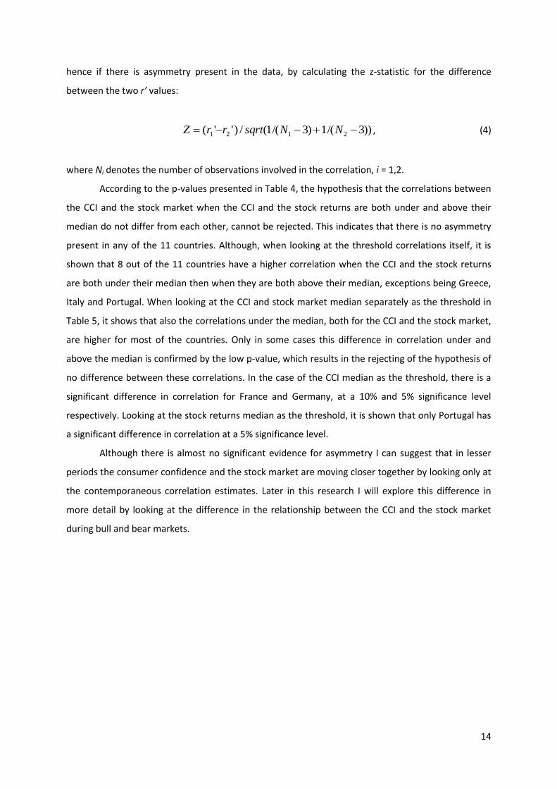
To ensure stationarity, I transform the variables. I perform different unit root tests to
examine if there is a unit root present, hence the time series are non-stationary. Table 2 shows the
results of the Augmented Dickey-Fuller (ADF) test and Phillips-Perron test. Panel A provides the ADF
test statistic and its p-value as well as the Phillips-Perron test statistic and its p-value for the CCI of
the 11 countries. Panel B presents the same test results for the natural logarithm (ln) of the stock
indices. The ln transformation is a common transformation when working with economic data that
includes a trend, it substitutes an exponential trend by a linear trend. The two tests are conducted
including a constant for the consumer confidence indices and including a constant and a trend for the
stock indices. Panel A shows that when looking at the ADF test statistics and its p-values the unit root
hypothesis cannot be rejected at a 1% significance level for most of the CCI time series, the only
exception being Germany. But the Phillip-Perron test indicates that rejection of the unit root is not
possible for Germany as well at a 1% significance level. Although, Davidson and MacKinnon (2004)
report that the Phillips-Perron test performs worse than the ADF test in finite samples, I still put the
same restriction on the CCI for Germany. Because the CCI time series of most of the countries
contain a unit root, I(1), I take the first differences of the time series to make them stationary4. Panel
B illustrates that for all the (ln) stock indices the unit root hypothesis cannot be rejected at a 1%
significance level. I also take the first differences of the natural logarithm of the stock indices to make
them stationary4.
Table 2: ADF and Phillip-Perron test
This table shows the test statistics and p-values of the Augmented Dickey-Fuller (ADF) and Phillip-Perron test of the CCI, shown in Panel A, and of the log stock indices (ln(SI)), shown in Panel B, for the 11 countries over the period January 1985 to June 2012. The tests for the CCI include only a constant. While the tests for the ln(SI) include a constant and a trend.
4 Table A.1 in the Appendix shows that after taking the first differences of the CCI and of the natural logarithm
of the stock indices the time series do not show a unit root any longer.
Belgium Denmark France Germany Greece Ireland Italy Netherlands Portugal Spain UK
Furthermore, the Johansen Cointegration Trace test indicates no cointegration at a 1%
significance level for all the 11 countries5. Which means there is no indication for a long term
relationship between the CCI and the stock market.
To make the CCI and stock index variables comparable I standardize them. Variables
measured at different scales do not contribute equally to the analysis. Data standardization
procedures equalize the range and/or data variability. I standardize the CCI and stock index data
series by dividing each variable by its standard deviation. This method produces a set of transformed
variables with variances of 1, but different means and ranges.
5 See Table A.2 in the Appendix for the Johansen Cointegration Trace test results.
12
3 Correlation
This section describes the correlation analysis for the full data sample, January 1985 until
June 2012. The first step in analyzing the relationship between (two) variables is to look at their
correlation. Although an observed correlation does not allow one to say anything about causation
between the variables, it is a good way to get a first notion of their relationship.
3.1 Dynamic correlation
To get a first impression of the relationship between (changes in) consumer confidence (CCI)
and (changes in) the stock market (SI) I look at the contemporaneous correlation between these two
time series6. The fourth column of Table 3 shows that the contemporaneous correlation (j=0)
between the CCI and the associated stock index is positive and significant for all the countries, which
means that the stock market and consumer confidence have a tendency to move in the same
direction. The contemporaneous correlation estimates have a range from 0.181-0.339, where
Belgium features the highest, and Denmark features the lowest contemporaneous correlation
estimate. The contemporaneous correlation analysis indicates that there is a positive relationship
between consumer confidence and the stock market. But it does not say anything about the
direction of this relationship. Does a higher stock price cause an improvement in consumer
confidence, or does an improvement in the consumer confidence cause higher stock prices. The
causality could also run in both directions.
To obtain an enhanced first impression Table 3 reports also the dynamic cross-correlations.
The fifth column shows that besides the significant contemporaneous correlations, the CCI and 1-
month lagged stock index are significantly correlated as well for all the 11 countries. Although these
correlation estimates are lower than the contemporaneous correlations, except for the Netherlands,
this does indicate that the direction of the causality runs from the stock market to the CCI and not
the other way around. The few significant correlations in the last two columns also confirm this
direction of the relationship. When considering the causality direction from the CCI to the stock
market, by looking at the dynamic correlations presented in columns 1-3, there is very low and
almost no significant correlations presented. The fact that the contemporaneous correlations are the
highest of all, indicates that the stock market has an effect on the CCI almost at the same time, or by
all means in a time frame of less than a month. 6 From now on I will use the terms consumer confidence or CCI and stock market/stock index or SI. In section 2
is explained that I mean by the consumer confidence, the first differences of the Consumer Confidence Index (∆CCI). The stock market is defined as the fist differences of the natural logarithm of the stock index (∆ln(SI)). Both variables are standardized by dividing them by their own standard deviation.
13
Table 3: Dynamic correlation
This table presents the dynamic correlation estimates of the consumer confidence, CCI(t) and the associated stock market, SI(t-j), of the 11 countries, for j = -3,…,3. The superscripts (***), (**) and (*) indicate statistical significance at a 1%, 5% and 10% level respectively. The sample period runs from January 1985 to June 2012.
3.2 Threshold correlation
To say something about the asymmetry of the relationship between the CCI and the stock
market I look at a so called ‘threshold correlation’. As threshold I take the median of the CCI and the
stock return. I calculate the correlation between the CCI and the stock market when the CCI and
stock index are both below their median, and the correlation when the CCI and stock index are both
above their median, these results are presented in Table 4. As a robustness check Table 5 shows the
correlations when I look at the median threshold separately for the CCI and the stock market. Hence,
looking at the correlation between the CCI and stock index when the CCI values are under/above the
CCI median, regardless of the stock index values. The same method performed for the stock index as
the threshold, regardless of the CCI value.
To test if the correlation under the median is significantly different from the correlation
above the median Fisher’s transformation of the correlation coefficient is used:
r
rr
1
1ln
2
1' , (3)
where r denotes the correlation coefficient. This transformation produces a function that is normally
distributed. Thereafter I test whether the two correlations are significantly different from each other,
UK -0.036 0.057 0.062 0.220*** 0.152*** -0.030 0.013
Correlation CCI(t) and SI(t-j)
14
hence if there is asymmetry present in the data, by calculating the z-statistic for the difference
between the two r’ values:
))3/(1)3/(1(/)''( 2121 NNsqrtrrZ , (4)
where Ni denotes the number of observations involved in the correlation, i = 1,2.
According to the p-values presented in Table 4, the hypothesis that the correlations between
the CCI and the stock market when the CCI and the stock returns are both under and above their
median do not differ from each other, cannot be rejected. This indicates that there is no asymmetry
present in any of the 11 countries. Although, when looking at the threshold correlations itself, it is
shown that 8 out of the 11 countries have a higher correlation when the CCI and the stock returns
are both under their median then when they are both above their median, exceptions being Greece,
Italy and Portugal. When looking at the CCI and stock market median separately as the threshold in
Table 5, it shows that also the correlations under the median, both for the CCI and the stock market,
are higher for most of the countries. Only in some cases this difference in correlation under and
above the median is confirmed by the low p-value, which results in the rejecting of the hypothesis of
no difference between these correlations. In the case of the CCI median as the threshold, there is a
significant difference in correlation for France and Germany, at a 10% and 5% significance level
respectively. Looking at the stock returns median as the threshold, it is shown that only Portugal has
a significant difference in correlation at a 5% significance level.
Although there is almost no significant evidence for asymmetry I can suggest that in lesser
periods the consumer confidence and the stock market are moving closer together by looking only at
the contemporaneous correlation estimates. Later in this research I will explore this difference in
more detail by looking at the difference in the relationship between the CCI and the stock market
during bull and bear markets.
15
Table 4: Threshold correlation, both CCI and SI under/above their median
This table presents the threshold correlation estimates and the associated z-statistics and p-values for comparing the correlation between the CCI and the stock market when the CCI and the stock index are both under their median and when they are both above their median for the 11 countries. The sample period runs from January 1985 to June 2012.
Table 5: Threshold correlation, separately for CCI and SI under/above their median
This table presents the threshold correlation estimates and the associated z-statistics and p-values for comparing the correlation between the CCI and the stock market when the CCI is under and above its median, and when the stock index is under and above its median, for the 11 countries. The sample period runs from January 1985 to June 2012.
Under median Above median z-statistic p-value
Belgium 0.369 0.251 0.814 0.416
Denmark 0.281 0.249 0.210 0.834
France 0.337 0.105 1.596 0.111
Germany 0.208 0.033 1.180 0.238
Greece 0.194 0.254 -0.314 0.753
Ireland 0.178 0.045 0.864 0.388
Italy 0.131 0.338 -1.463 0.143
Netherlands 0.168 0.141 0.187 0.852
Portugal 0.188 -0.035 1.241 0.215
Spain 0.214 0.167 0.319 0.749
UK 0.179 0.210 -0.219 0.827
Threshold correlation
Under median Above median z-statistic p-value Under median Above median z-statistic p-value
UK 0.263 0.109 -1.299 0.194 0.212 0.125 -0.725 0.468
SICCI
16
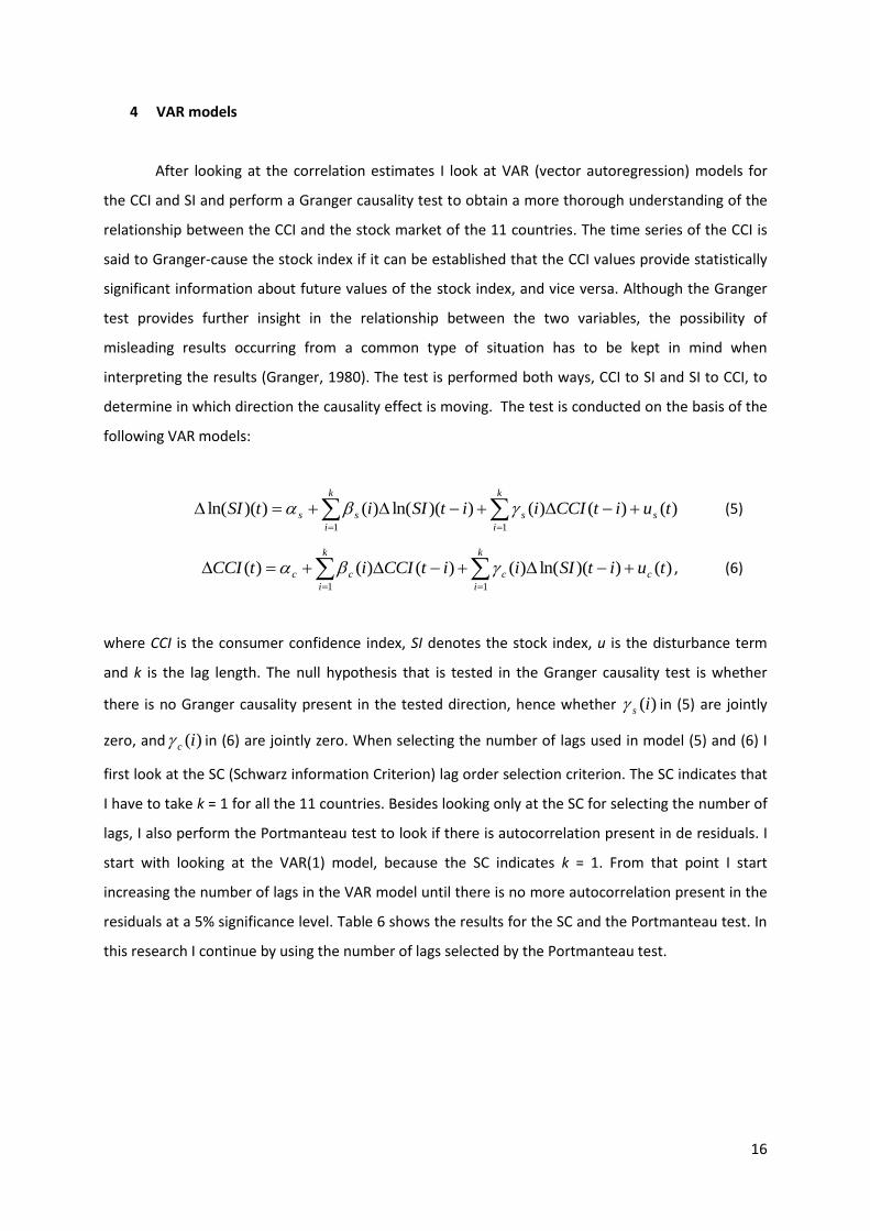
4 VAR models
After looking at the correlation estimates I look at VAR (vector autoregression) models for
the CCI and SI and perform a Granger causality test to obtain a more thorough understanding of the
relationship between the CCI and the stock market of the 11 countries. The time series of the CCI is
said to Granger-cause the stock index if it can be established that the CCI values provide statistically
significant information about future values of the stock index, and vice versa. Although the Granger
test provides further insight in the relationship between the two variables, the possibility of
misleading results occurring from a common type of situation has to be kept in mind when
interpreting the results (Granger, 1980). The test is performed both ways, CCI to SI and SI to CCI, to
determine in which direction the causality effect is moving. The test is conducted on the basis of the
following VAR models:
)()()())(ln()())(ln(11
tuitCCIiitSIitSI s
k
i
s
k
i
ss
(5)
)())(ln()()()()(11
tuitSIiitCCIitCCI c
k
i
c
k
i
cc
, (6)
where CCI is the consumer confidence index, SI denotes the stock index, u is the disturbance term
and k is the lag length. The null hypothesis that is tested in the Granger causality test is whether
there is no Granger causality present in the tested direction, hence whether )(is in (5) are jointly
zero, and )(ic in (6) are jointly zero. When selecting the number of lags used in model (5) and (6) I
first look at the SC (Schwarz information Criterion) lag order selection criterion. The SC indicates that
I have to take k = 1 for all the 11 countries. Besides looking only at the SC for selecting the number of
lags, I also perform the Portmanteau test to look if there is autocorrelation present in de residuals. I
start with looking at the VAR(1) model, because the SC indicates k = 1. From that point I start
increasing the number of lags in the VAR model until there is no more autocorrelation present in the
residuals at a 5% significance level. Table 6 shows the results for the SC and the Portmanteau test. In
this research I continue by using the number of lags selected by the Portmanteau test.
17
Table 6: Lag selection
This table presents the number of lags that are selected for each of the 11 countries. The first column shows the results when looking at the Schwarz information Criterion (SC). The second column presents the number of lags when looking at the Portmanteau test for the presence of autocorrelation in the residuals. The selected number of the Portmanteau lags comes from the procedure of increase the VAR model until there is no more autocorrelation present in the residuals at a 5% significance level. The sample period runs from January 1985 to June 2012.
4.1 Full sample results
First I am analyzing the Granger causality of the full sample, January 1985 until June 2012.
Table 7 reports the p-values of the test statistics for the Granger causality test in both directions, CCI
to SI and SI to CCI. There is no Granger causality present from the CCI to the stock indices for all the
countries. This confirms the findings of the dynamic correlations analysis. However, for the majority
of the countries the stock indices Granger cause the CCI, the only exception being Portugal. For
Belgium, France, Germany, Ireland, Italy, the Netherlands, Spain and the UK I find statistically
significant Granger causality at a 1% significance level, for Denmark at a 5% significance level, and for
Greece at a 10% significance level. These results indicate that the publication of the consumer
survey data (at the end of each month) does not have a significant effect on the stock market. But
the stock market does have, for most of the countries (although for different significance levels), an
effect on the consumer confidence.
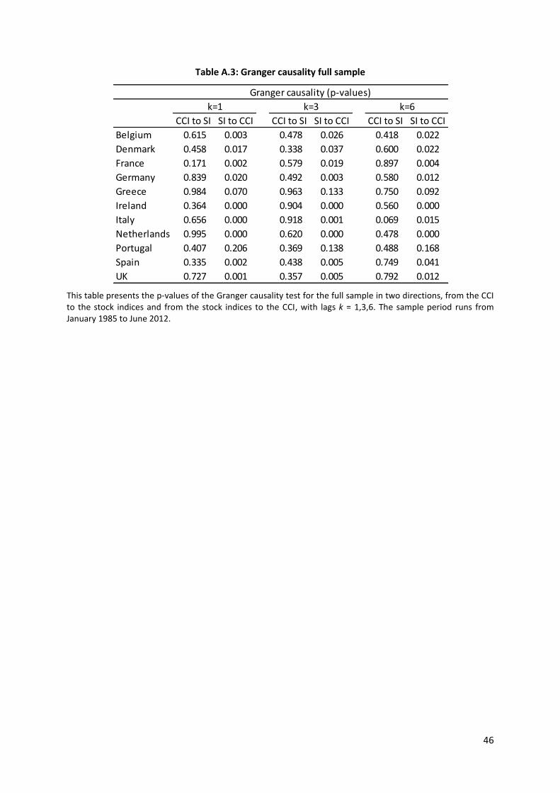
As a robustness check I also look at the Granger causality for the same number of lags for all
the countries, k = 1, 3 and 6. Table A.3 in the Appendix does not show large differences with the
results in Table 7.
Lag order criteria Autocorrelation residual test
SC Portmanteau
Belgium 1 1
Denmark 1 2
France 1 1
Germany 1 2
Greece 1 1
Ireland 1 2
Italy 1 3
Netherlands 1 4
Portugal 1 1
Spain 1 2
UK 1 1
18
Table 7: Granger causality full sample
This table presents the Granger causality p-values for the full sample running from January 1985 to June 2012. The Granger causality test is performed in two directions, from the CCI to the stock indices and from the stock indices to the CCI. The number of lags used are different per country depending of the outcome of the Portmanteau test, see table 6.
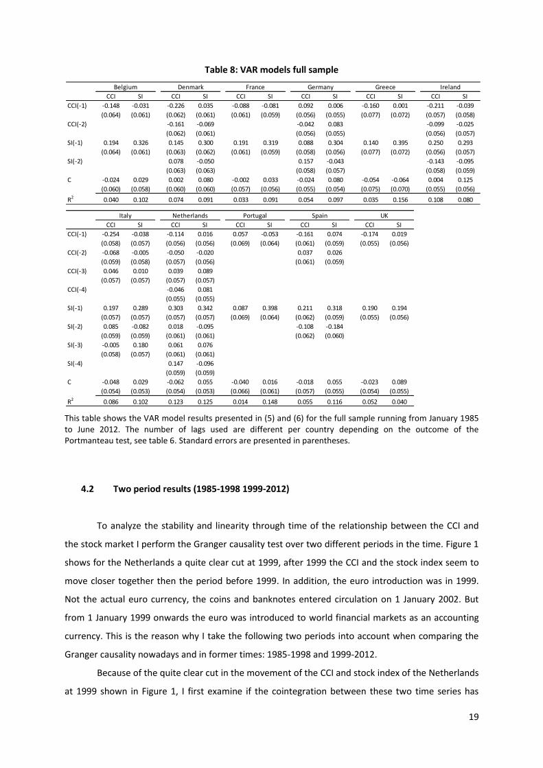
When looking at the results of the different VAR models in Table 8, and especially to the signs
of the coefficients, it again becomes clear that the causality effect is running from the stock market
to the CCI. Mainly in equation (6) this corresponds to the fact that the one month lagged stock
indices (SI(-1)) are positive for all the countries, with a range from 0.087 for Portugal to 0.303 for the
Netherlands. When looking at the higher lags, which are included only for some countries depending
on the outcome of the Portmanteau test, I see that these coefficients are not always positive and
they are less high then the SI(-1) coefficients, except for Germany. The one month lagged CCI in
equation (5) are all around 0, ranging from -0.081 for France to 0.074 for Spain. The same results are
found when looking at higher lags for the CCI. These findings can be interpreted again as evidence
that the causality is running from the stock market to the CCI instead of from the CCI to the stock
market.
The coefficients of determination (R2) are all very low, this means that not much variation of
the dependent variable can be attributed to differences in the explanatory variables. In most cases
model (5) shows a higher R2 then model (6), except for Ireland and Spain. This is probably due to the
fact that the SI(-1) coefficients show a high value in model (5). Hence, the stock index from one
month ago has an influence on the stock index now.
CCI to SI SI to CCI
Belgium 0.615 0.003
Denmark 0.380 0.013
France 0.171 0.002
Germany 0.304 0.002
Greece 0.984 0.070
Ireland 0.761 0.000
Italy 0.918 0.001
Netherlands 0.330 0.000
Portugal 0.407 0.206
Spain 0.442 0.002
UK 0.727 0.001
Granger causality (p-values)
19
Table 8: VAR models full sample
This table shows the VAR model results presented in (5) and (6) for the full sample running from January 1985 to June 2012. The number of lags used are different per country depending on the outcome of the Portmanteau test, see table 6. Standard errors are presented in parentheses.
4.2 Two period results (1985-1998 1999-2012)
To analyze the stability and linearity through time of the relationship between the CCI and
the stock market I perform the Granger causality test over two different periods in the time. Figure 1
shows for the Netherlands a quite clear cut at 1999, after 1999 the CCI and the stock index seem to
move closer together then the period before 1999. In addition, the euro introduction was in 1999.
Not the actual euro currency, the coins and banknotes entered circulation on 1 January 2002. But
from 1 January 1999 onwards the euro was introduced to world financial markets as an accounting
currency. This is the reason why I take the following two periods into account when comparing the
Granger causality nowadays and in former times: 1985-1998 and 1999-2012.
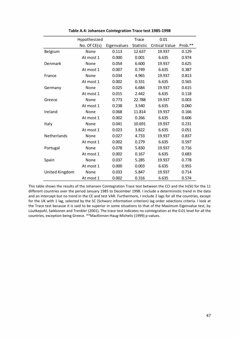
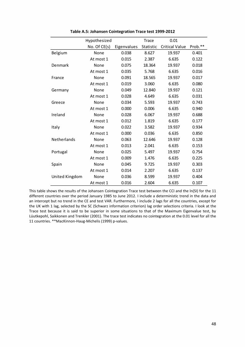
Because of the quite clear cut in the movement of the CCI and stock index of the Netherlands
at 1999 shown in Figure 1, I first examine if the cointegration between these two time series has
changed in the two periods. Table A.4 and A.5 in the Appendix show that the Johansen Cointegration
Trace test for the CCI and ln(SI) indicates no cointegration at a 1% significance level for all the
countries, exception being Greece in the first period. This could be explained by the fact that the
Greece time series runs from September 1997. Consequently, in the first period only 15 observations
are included, which is too short a period to obtain statistically significant results.
The contemporaneous correlation results in Table 9 show that most countries have an
increased correlation between the CCI and the stock market in the second period, 1999-2012. The
exceptions here are Italy, Spain and the UK. The average correlation is 0.194 in 1985-1998, and 0.273
in 1999-2012. This is a small but visible increase. While Greece had the lowest correlation in the first
period, the UK has the lowest correlation in the second period. The highest correlation in the first
period is in Spain, while the highest correlation in the second period is in France. Although the
average contemporaneous correlation between the CCI and SI is higher in the second period. The
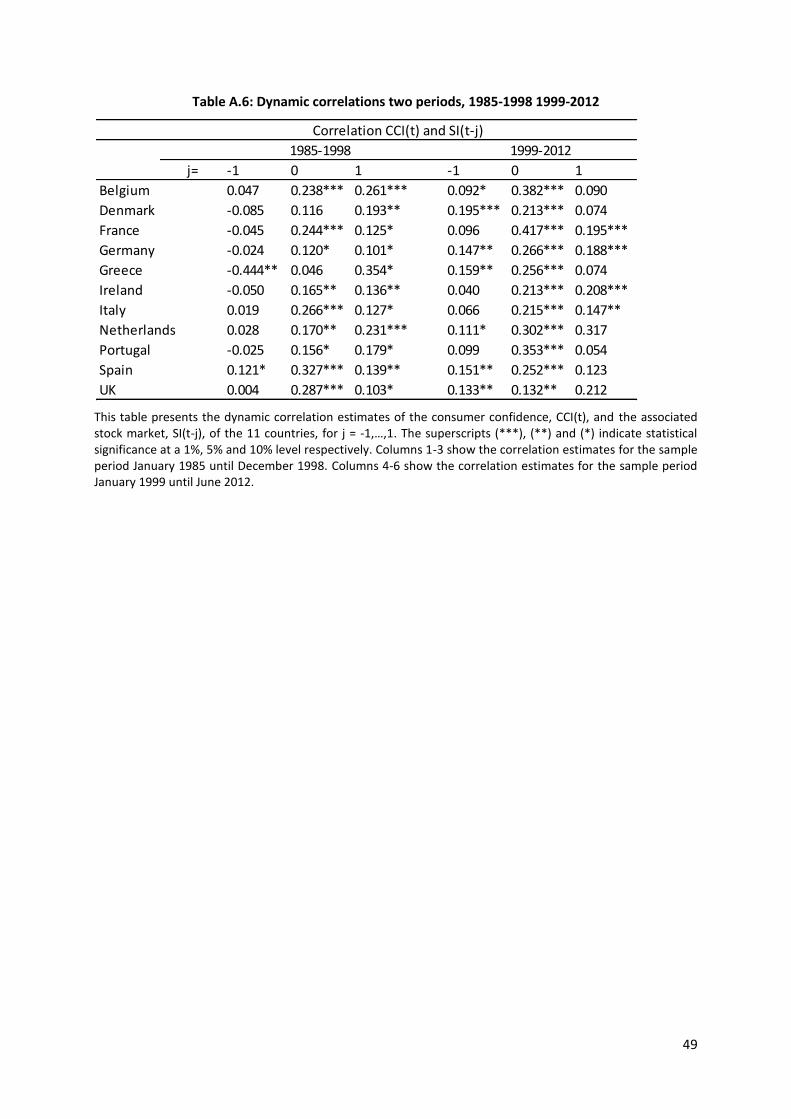
dynamic correlations in Table A.6 in the Appendix show that in this second period most of the
correlations between the 1 month lagged SI and the CCI are not significant anymore.
Table 9: Correlation and Granger causality two periods, 1985-1998 1999-2012
This table presents in columns 1-2 the contemporaneous correlation estimates of the CCI and the associated stock index of the 11 countries. The superscripts (***), (**) and (*) indicate statistical significance at a 1%, 5% and 10% level respectively. Columns 3-6 report the p-values of the Granger causality test in two directions, from the CCI to the stock indices and from the stock indices to the CCI. The number of lags used are different per country depending on the outcome of the Portmanteau test, see table 6. Column 1, 3 and 4 show the results for the sample period January 1985 until December 1998. Column 2, 5 and 6 show the results for the sample period January 1999 until June 2012.
Table 9 also shows the results of the Granger causality test for years in the past and in former times.
Columns 3 and 4 cover the period from January 1985 until December 1998. The results indicate that
1985-1998 1999-2012
Estimate Estimate CCI to SI SI to CCI CCI to SI SI to CCI
Greece is the only country with Granger causality that runs from the CCI to the stock index at a 10%
significance level. This could again be explained by the fact that the Greece time series only has 15
observations in the first period, which is too short a period to obtain statistically significant results.
Furthermore, for Greece there is no Granger causality from the stock index to the CCI in this period.
Also, Germany and Portugal show no Granger causality from the stock index to the CCI. Whereas, I
find statistically significant Granger causality that runs from the stock index to the CCI for Belgium
and Spain at a 1% significance level, for Italy and the Netherlands at a 5% significance level, and for
Denmark, France, Ireland and the UK at a 10% significance level. Columns 5 and 6 show the results
for the second period, January 1999 until June 2012. In this period there is no Granger causality
present from the CCI to the stock indices for most of the countries again, except for Germany at a 5%
significance level and for Denmark at a 10% significance level. Also, there is no Granger causality
present from the stock indices to the CCI for Greece, Portugal and Spain. For the other countries the
stock index does Granger cause the CCI: Germany, Ireland, the Netherlands and the UK at a 1%
significance level, and Belgium, Denmark, France and Italy at a 5% significance level.
Although the average contemporaneous correlation increased considerably in the second
period, the results from the Granger causality test do not indicate that there is an overall difference
between the two periods. The results for the Granger causality running from the CCI to the stock
market stay more or less the same for both periods. The Granger causality running from the stock
market to the CCI changes slightly for some countries. While the p-values of the Granger causality
test for Portugal (0.140) and Spain (0.005) indicated the presence of causality in the first period, this
significant causality is not present anymore in the second period, with p-values of 0.862 for Portugal
and 0.204 for Spain. For Germany it is the other way around. In the first period there is no Granger
causality present from the stock market to the CCI with a p-value of 0.496, but in the second period
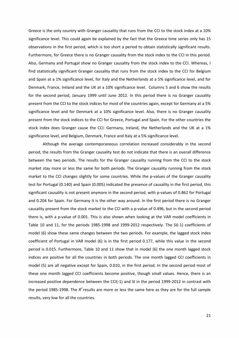
there is, with a p-value of 0.001. This is also shown when looking at the VAR model coefficients in
Table 10 and 11, for the periods 1985-1998 and 1999-2012 respectively. The SI(-1) coefficients of
model (6) show these same changes between the two periods. For example, the lagged stock index
coefficient of Portugal in VAR model (6) is in the first period 0.177, while this value in the second
period is 0.015. Furthermore, Table 10 and 11 show that in model (6) the one month lagged stock
indices are positive for all the countries in both periods. The one month lagged CCI coefficients in
model (5) are all negative except for Spain, 0.010, in the first period. In the second period most of
these one month lagged CCI coefficients become positive, though small values. Hence, there is an
increased positive dependence between the CCI(-1) and SI in the period 1999-2012 in contrast with
the period 1985-1998. The R2 results are more or less the same here as they are for the full sample
results, very low for all the countries.
22
Table 10: VAR models 1985-1998
This table shows the VAR model results presented in (5) and (6) for the sample running from January 1985 to December 1998. The number of lags used are different per country depending on the outcome of the Portmanteau test, see table 6. Standard errors are presented in parentheses.
This table shows the VAR model results presented in (5) and (6) for the sample running from January 1999 to June 2012. The number of lags used are different per country depending on the outcome of the Portmanteau test, see table 6. Standard errors are presented in parentheses.
4.3 Bull and bear markets
Besides looking at the overall relationship between the CCI and the stock market and
analyzing the stability and linearity of this relationship through time, I also explore if the relationship
changes in different stages of the economy. Because I am working with stock prices, I look if the
relationship between the CCI and the stock market is different in bull markets compared to bear
markets. Although there is not a clear definition of bull and bear markets, a bull market is commonly
distinguished as a prolonged period of rising stock prices, while a bear market is characterized by
falling prices and higher volatility. The stock market changes from a bull to a bear state if prices
decline for a substantial period and with a substantial value since their previous (local) peak. This
definition does not rule out sequences of negative (positive) price movements during bull (bear)
markets. How large price increases or decreases should be, or how long rising or falling tendencies
should last is not uniquely specified. Because of the absence of a clear definition the academic
literature does not offer a single preferred method to identify bullish and bearish periods. Kole and
van Dijk (2010) analyze different methods that have been put forward in the academic literature to
indentify and predict bull and bear markets. By looking at their results I choose to use the algorithm
described by Lunde and Timmerman (2004) to identify bullish and bearish periods in the stock
market data for the 11 European countries. I choose this algorithm because it is a transparent
method and Kole and van Dijk (2010) show that this method, although I only use the identification
part of the algorithm, results in the best investment performance.
The Lunde and Timmerman (2004) approach focus on local peaks and troughs. Between a
trough and a subsequent peak there is a bull market, and between a peak and a subsequent trough
there is a bear market. Let λ be a scalar defining the threshold of the movements in the stock index
that triggers a switch between bull and bear markets. A bull market occurs when the stock index has
increased by at least λ1 since the last trough. A bear market occurs when the stock index has
decreased by at least λ2 since the last peak. I follow Linde and Timmerman (2004) by setting λ1 = 0.20
and λ2 = 0.15. Hence, an increase of 20% of the stock index over the last trough indicates a bull
market, and a decrease of 15% of the stock market over the last peak specifies a bear market. The
algorithm to identify peaks and troughs in a time series is summarized as follows:
1. The last observed extreme value is a peak with stock index value Pmax. The subsequent period
is considered.
(i) If the stock index exceeds the last maximum, the maximum is updated (if SI > Pmax,
then Pmax = SI).
(ii) If the stock index drops with a fraction λ2, a trough is found (if SI < (1 - λ2) Pmax, then
Pmin = SI).
(iii) If neither of the conditions is satisfied, no update takes place.
2. The last observed extreme value is a trough with stock index value Pmin. The subsequent
period is considered.
(i) If the stock index drops below the last minimum, the minimum is updated (if
SI < Pmin, then Pmin = SI).
(ii) If the stock index increases with a fraction λ1, a peak is found (if SI > (1 + λ1) Pmin, then
Pmax = SI).
(iii) If neither of the conditions is satisfied, no update takes place.
25
Like Kole and van Dijk (2010) I distinguish whether the market is initially a bull or a bear market by
counting the number of times the maximum and minimum has to be adjusted since the first
observation. If the maximum has to be adjusted three times first instead of the minimum three times
first, I consider the market to be bullish initially, otherwise the market is initially bearish.
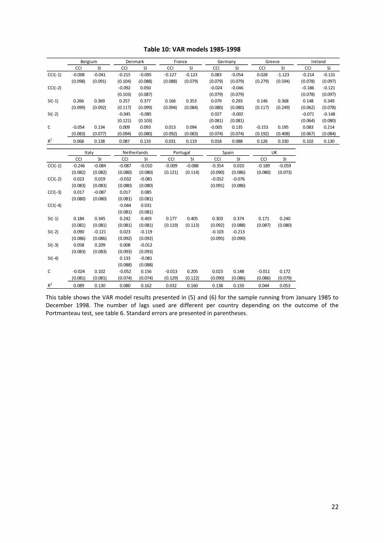
Table 12: Number and duration of bull and bear markets
This table shows for the bull and bear market the number of spells, their average and median duration and the standard deviation of the duration. It also reports to total number of observations in all the bull (bear) markets. The algorithm that is used to identify the bull and bear markets is the Lunde and Timmerman (2004) algorithm. The sample period runs from January 1985 to June 2012.
This figure shows the identification of bull and bear market periods in the Netherlands over the period January 1985 to June 2012. The algorithm that is used to identify the bull and bear markets is the Lunde and Timmerman (2004) algorithm. The thin black line plots the Dutch stock market index, the AEX, and the thick black line plots the CCI of the Netherlands. Purple areas indicate bear markets, and white areas correspond with bull markets.
Figure 2 shows the CCI and stock market of the Netherlands, and the state of the market. The
purple areas correspond with bear markets, and white areas indicate bull markets. The familiar
financial landmarks are all present; the well known bearish periods in 1987 and 1989-1990, the burst
of the IT-bubble in 2000 and the resent credit crunch started in 2007. Besides these big bearish
Belgium Denmark France Germany Greece Ireland Italy Netherlands Portugal Spain UK
total number of observations 104 91 112 78 98 87 155 105 120 132 63
26
periods, there is a shorter period with sustained declines in the AEX, August 1998-October 1998,
which possibly is a consequence of the Russian financial crisis that was going on at that time. The
figure shows that during bear (bull) markets the CCI ad the stock market move together in a
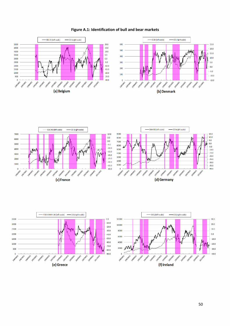
downward (upward) slope. The recession in 1992/93 is not identified as a bear market. While the
stock market stays more or less the same in this period, the CCI declines significantly. Figure A.1 in
the Appendix reports for the other 12 countries the bull/bear market identification graphs. All the
countries show more or less the same bear markets that are described for the Netherlands,
exceptions being a few small bear periods that are illustrated for some countries.
Table 13: Dynamic correlations bull and bear markets
This table presents the dynamic correlation estimates of the consumer confidence, CCI(t), and the associated stock market, SI(t-j), of the 11 countries, for j = -1,…,1. The superscripts (***), (**) and (*) indicate statistical significance at a 1%, 5% and 10% level respectively. Columns 1-3 show the correlation estimates for when the state of the economy is considered to be a bull market. Columns 4-6 show the correlation estimates for when the state of the economy is considered to be a bear market. The algorithm that is used to identify bull and bear markets is the Lunde and Timmerman (2004) algorithm. The sample period runs from January 1985 to June 2012.
The contemporaneous correlation estimates in Table 13 show that for most of the countries
the bear market correlation estimates are higher than the bull market correlation estimates,
exceptions being Germany, Italy and the UK. Also, the average correlation of all the countries when
the state of the economy is considered to be a bear market, 0.221, is higher than when the state of
the economy is considered to be a bull market, 0.153. However, when looking at the dynamic
correlations and Granger causality results there is no similar difference in bull and bear markets
recognized. The dynamic correlation estimates in Table 13 show that for most of the countries there
is a higher and significant correlation estimate when j = 1 opposed to j = -1 for both the bear and bull
markets. This indicates once again that the causality running from the stock market to the CCI is
stronger than the other way around. But there is no difference between the bear and bull market
dynamic correlation analysis, both states of the economy show more or less the same results. From
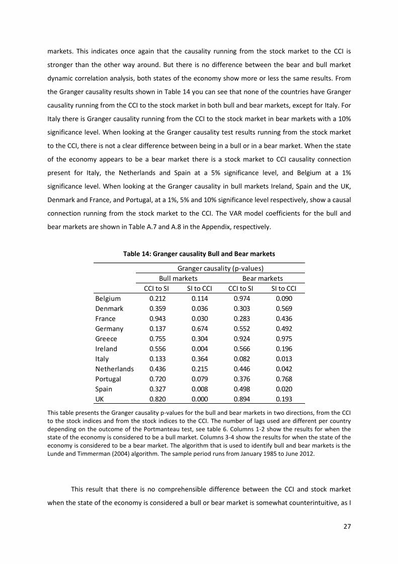
the Granger causality results shown in Table 14 you can see that none of the countries have Granger
causality running from the CCI to the stock market in both bull and bear markets, except for Italy. For
Italy there is Granger causality running from the CCI to the stock market in bear markets with a 10%
significance level. When looking at the Granger causality test results running from the stock market
to the CCI, there is not a clear difference between being in a bull or in a bear market. When the state
of the economy appears to be a bear market there is a stock market to CCI causality connection
present for Italy, the Netherlands and Spain at a 5% significance level, and Belgium at a 1%
significance level. When looking at the Granger causality in bull markets Ireland, Spain and the UK,
Denmark and France, and Portugal, at a 1%, 5% and 10% significance level respectively, show a causal
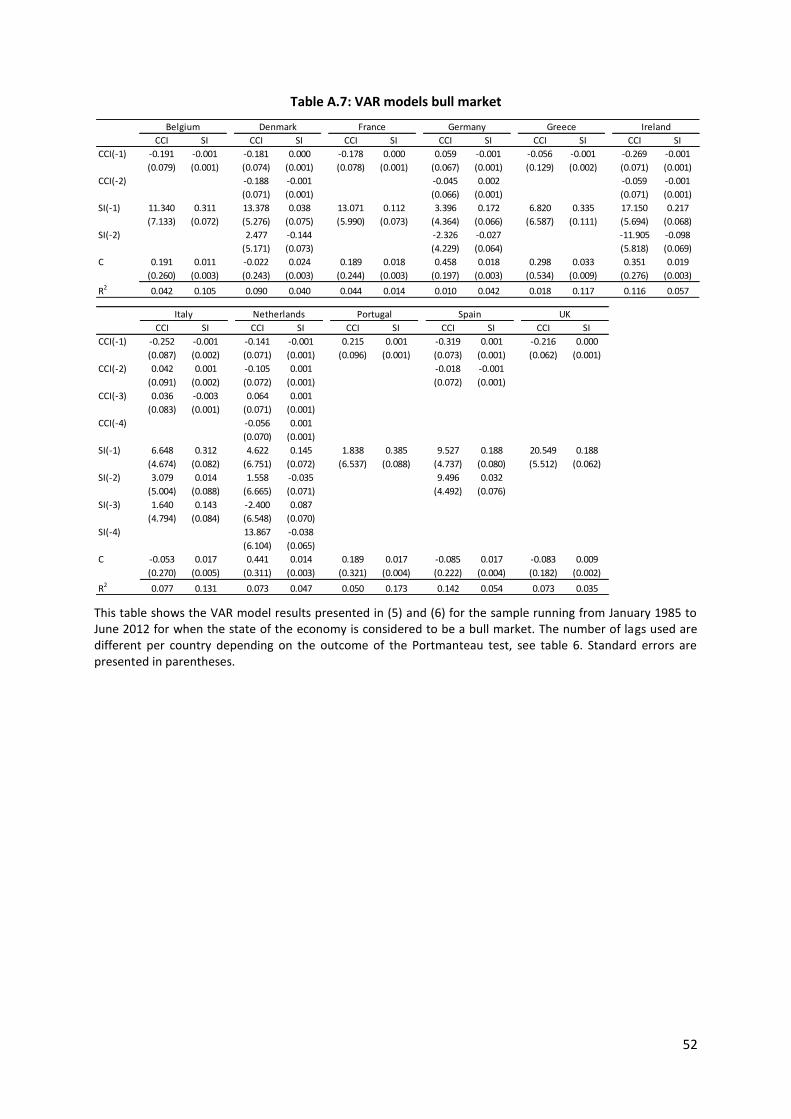
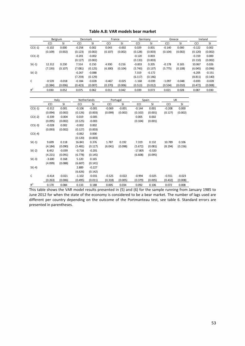
connection running from the stock market to the CCI. The VAR model coefficients for the bull and
bear markets are shown in Table A.7 and A.8 in the Appendix, respectively.
Table 14: Granger causality Bull and Bear markets
This table presents the Granger causality p-values for the bull and bear markets in two directions, from the CCI to the stock indices and from the stock indices to the CCI. The number of lags used are different per country depending on the outcome of the Portmanteau test, see table 6. Columns 1-2 show the results for when the state of the economy is considered to be a bull market. Columns 3-4 show the results for when the state of the economy is considered to be a bear market. The algorithm that is used to identify bull and bear markets is the Lunde and Timmerman (2004) algorithm. The sample period runs from January 1985 to June 2012.
This result that there is no comprehensible difference between the CCI and stock market
when the state of the economy is considered a bull or bear market is somewhat counterintuitive, as I
CCI to SI SI to CCI CCI to SI SI to CCI
Belgium 0.212 0.114 0.974 0.090
Denmark 0.359 0.036 0.303 0.569
France 0.943 0.030 0.283 0.436
Germany 0.137 0.674 0.552 0.492
Greece 0.755 0.304 0.924 0.975
Ireland 0.556 0.004 0.566 0.196
Italy 0.133 0.364 0.082 0.013
Netherlands 0.436 0.215 0.446 0.042
Portugal 0.720 0.079 0.376 0.768
Spain 0.327 0.008 0.498 0.020
UK 0.820 0.000 0.894 0.193
Granger causality (p-values)
Bull markets Bear markets
28
expected to find more significant values of Granger causality in the bear markets than in the bull
markets. This is due to the fact that the contemporaneous correlation estimates show higher values
in the bear markets. On the contrary, the dynamic correlation estimates do not show different
results for being in a bull or a bear market. Next to that, the threshold correlation results in section
3.2 show that there is a higher contemporaneous correlation when CCI and/or stock indices are
below their median. Although this is a sign that the CCI and the stock index move closer together in
lesser periods, it is not fully comparable to the economy being in a bear market. Because a bear
market is the period measured from a peak to a through, whereas the threshold correlation is
measured under the median. An explanation for the Granger causality outcome could be that the
total number of observations in especially the bear markets is quite small, as can be seen in Table 12.
Also the average duration per bear market is fairly small. The small number of total observations in
the bear markets and the small number of observations per bear market limit the reliability of the
analysis.
29
5 Copulas
Another method to investigate the relationship between the CCI and the stock indices is to
model the dependence by using copulas. Copulas help in the understanding of dependence at a
deeper level and are very popular in statistical applications. They allow one to easily model and
estimate the distribution of random vectors by estimating the marginals and copula separately. The
marginal distribution functions describes the marginal distribution of each component and the
copula describes the dependence structure between the components. This method is first introduced
by Sklar (1959).
Theorem 1. Let ),...,( 1 nXXX be a random vector with cumulative distribution function
F and let iF denote the marginal distribution of iX , for ni ,...,1 . Then there exists a copula
]1,0[]1,0[: nC such that
))(,...),((),...,( 111 nnn xFxFCxxF . (7)
A copula C of the random vector X is thus a function that maps the univariate marginal
distributions nFF ,...,1 to the joint distribution F , and we write ),...,(~ 1 nFFCFX . If the
marginals iF are continuous, then C in (1) is unique and is given by
))(,...),((),...,( 1
1
1
11 nnn uFuFFuuC (8)
for n
n Ruuu ),...,( 1 where })(:inf{)( uxFxuF i
n
i .
Conversely, given any collection of univariate distributions nFF ,...,1 and any copula C , then F
defined by (7) defines a valid joint distribution with marginal distributions nFF ,...,1 .
In this paper, I consider a bivariate relationship, namely the relationship between the CCI and
the stock market. I use the symbols x and y ),( Ryx to denote the observations of the random
variables X and Y ; and u and v ])1,0[,( vu to denote their marginal cumulative distribution
functions (CDFs). The probability density function (PDF) of a bivariate copula ),( vuC is defined as
30
vu
vuCvuc
),(),( (9)
The density of the bivariate distribution ),( yxF can be written as the product of the copula density
and the marginal densities.
)()())(),((),( yfxfyFxFcyxf YXYX (10)
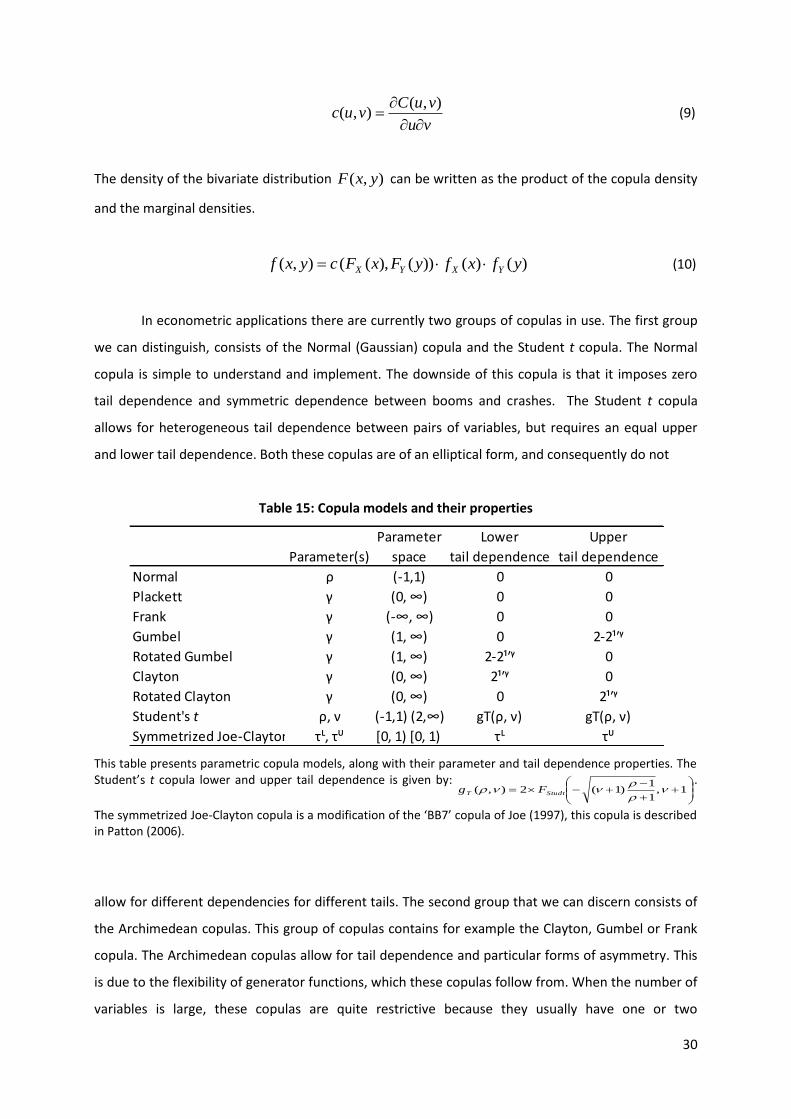
In econometric applications there are currently two groups of copulas in use. The first group
we can distinguish, consists of the Normal (Gaussian) copula and the Student t copula. The Normal
copula is simple to understand and implement. The downside of this copula is that it imposes zero
tail dependence and symmetric dependence between booms and crashes. The Student t copula
allows for heterogeneous tail dependence between pairs of variables, but requires an equal upper
and lower tail dependence. Both these copulas are of an elliptical form, and consequently do not
Table 15: Copula models and their properties
This table presents parametric copula models, along with their parameter and tail dependence properties. The Student’s t copula lower and upper tail dependence is given by:
1,
1
1)1(2),(
StudtT Fg
.
The symmetrized Joe-Clayton copula is a modification of the ‘BB7’ copula of Joe (1997), this copula is described in Patton (2006).
allow for different dependencies for different tails. The second group that we can discern consists of
the Archimedean copulas. This group of copulas contains for example the Clayton, Gumbel or Frank
copula. The Archimedean copulas allow for tail dependence and particular forms of asymmetry. This
is due to the flexibility of generator functions, which these copulas follow from. When the number of
variables is large, these copulas are quite restrictive because they usually have one or two
Parameter Lower Upper
Parameter(s) space tail dependence tail dependence
parameters to characterize the dependence between all variables. Table 15 presents a summary of
some common copula models and their properties. For a more detailed description and analysis of
copulas Joe(1997) and Nelsen (1999) can be consulted.
5.1 Empirical distribution function
When estimating the copula models I use the full sample period, January 1985 to June 2012.
The estimated standard residuals obtained from the estimated VAR models (5) and (6) are
transformed using the empirical distribution function (EDF), and I obtain the estimated probability
integral transform variable, itU :
T
t
itiT
F1
}ˆ{11
1)(ˆ , (11)
)ˆ(ˆˆitiit FU .
When estimating the copula in Section 5.3 this results in a semiparametric copula-based model as
explained in Patton (2012), using a nonparamemtric model for the marginal distributions, the EDF,
and a parametric model for the copula.
5.2 Nonparametric dependence measures
Before focusing on the copula models I am looking at the nonparametric dependence
measures7, quantile, tail and symmetric dependence, to get a better understanding of which copula
model is a good fit for the data.
Quantile dependence is a measure of the strength of the dependence between two variables
in the joint lower, or joint upper, tails. Quantile dependence provides a more detailed description of
the dependence structure of two variables than a scalar measure like linear correlation does. The
strength of the dependence between the two variables is estimated by moving from the center
7 No parametric assumptions are made for the copula and the marginal distribution functions. The dependence
estimates are obtained using the empirical copula:
m
j
jj
m vm
Ru
m
R
mvuC
1
21},{1
1),(ˆ , where 1 denotes
the indicator function, R1j and R2j are the ranks of the block maxima X*
lj and Y*
lj, , respectively, j = 1,…,m and l = n/m.
32
( 2/1q ) to the tails, and by comparing the left tail ( 2/1q ) to the right tail ( 2/1q ). Following
Patton (2012), the quantile dependence is defined as8:
12/1},,{1)1(
1
2/10},,{11
ˆ
1
21
1
21
qqUqUqT
qqUqUTq
T
t
tt
T
t
tt
q (12)
Tail dependence is an extreme events dependence. In this application upper (lower) tail
dependence measures the dependence between the CCI and the stock market when both the stock
market and the CCI experience very good (bad) times. A nonparametric estimator of tail dependence
considered in Frahm, et al. (2005) is the ‘log’estimator:
)1(log
}1,1{1)1(21log
2ˆ*
1
*
2
*
1
1*
q
qUqUTqT
t
tt
L
for 0* q (13)
)1(log
}1,1{1log
2ˆ*
1
*
2
*
1
1
q
qUqUTT
t
tt
U
for 0* q (14)
The choice of a threshold *q involves trading off the variance in the estimator (small threshold
values) against bias (large threshold values). The method in Frahm, et al. (2005) is used to choose this
threshold.
To get a better understanding about the symmetric dependence, I test for asymmetry jointly.
To do this the estimated quantile dependence measures are stacked into a vector of the form:
]',...,,[ˆ 221 pqq where jjp qq 1 , for pj ,...,2,1 . (15)
Then the following test can be conducted:
0:0 RH vs. 0: RHa (16)
where pp IIR :
8 This quantile definition is adapted to positively dependent variables.
33
Following from Rémillard (2010) that ),0()ˆ( VNT d and using that SV ,ˆ denotes the
bootstrap estimate of V , the following holds under 0H :
21
, )ˆ()'ˆ(')ˆ( p
d
S RRVRRT (17)
Information about quantile, tail and symmetric dependence is useful because many copula
models impose symmetric dependence (Normal and Student t copula), zero tail dependence (Normal
and Frank copula), or zero tail dependence in one of their tails (right for the Clayton copula and left
for the Gumbel copula).
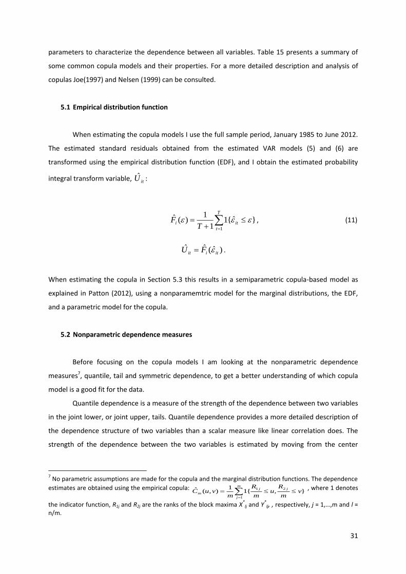
Figure 3: Quantile dependence results for the Netherlands
This figure shows the quantile dependence results for the Netherlands. Panel (a) presents the estimated quantile dependence between the residuals for the CCI and the SI, along with a 90% bootstrap confidence interval. Panel (b) presents the difference between the corresponding upper and lower quantile along with 90% bootstrap confidence interval for this difference. The sample period runs from January 1985 to June 2012.
Figure 3 presents the quantile dependence results for the Netherlands. Panel (a) shows the
estimated quantile dependence plot, for ]975.0,025.0[q , along with a 90% confidence interval,
calculated using a (pointwise) iid bootstrap approach. Panel (b) shows the difference between the
upper and lower quantile dependence fractions, with as well a 90% bootstrap confidence interval.
This figure shows that observations in the upper tail are slightly more dependent than observations
in the lower tail from q = 0.25 onwards, especially for the smallest quantile q = 0.025. Though the
confidence interval shows that these upper quantile dependence estimates are not as significant as
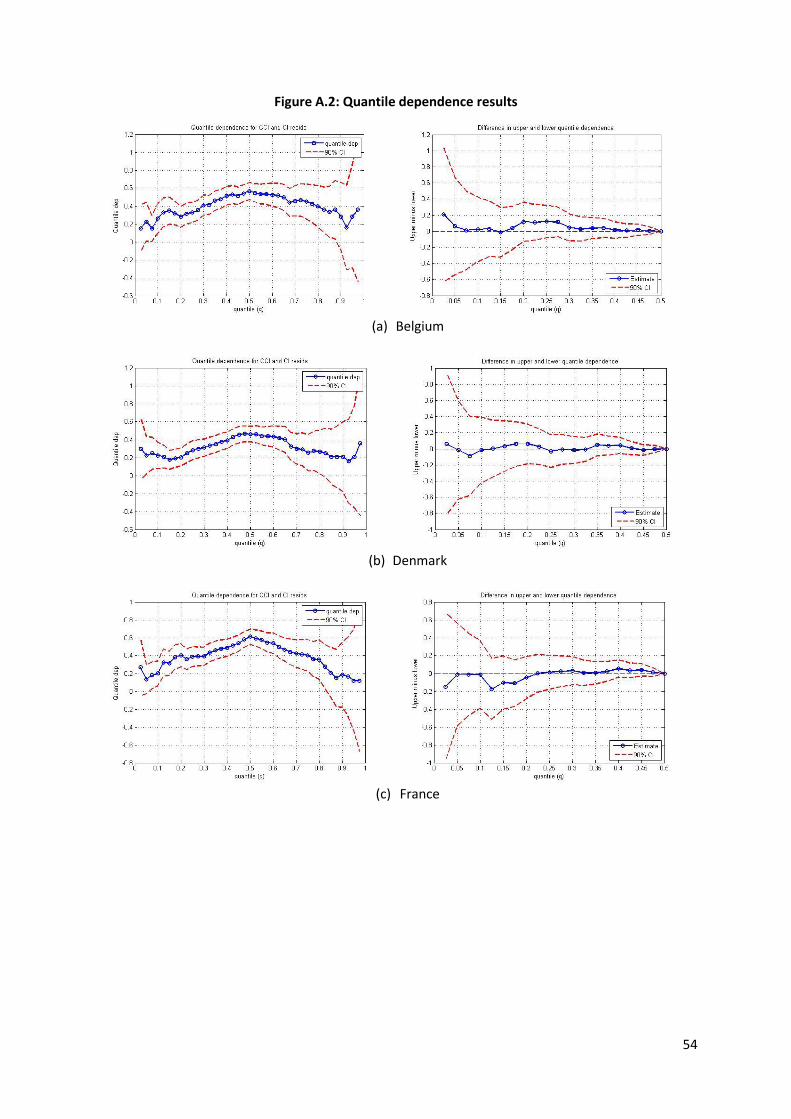
the rest of the quantile estimates. Figure A.2 in the Appendix shows the quantile graphs for the other
12 countries. There can be seen that all the countries show minor differences between the upper and
34
lower tail dependence, and slightly more difference in the smallest quantiles. Though this difference
in tail dependence is shown by the quantile dependence graphs, when looking at the upper and
lower tail dependence estimates presented in Table 16, I find that the tail dependence estimates are
rather low and also not significant. The 90% bootstrap confidence intervals indicate zero tail
dependence for both the lower and upper tail for roughly all the countries. Also, the large confidence
intervals yield less precise estimates of the lower and upper tail dependence. This could be expected
as Frahm, et al. (2005) states that nonparametric dependence estimates are sensitive in case of small
sample sizes like 250 data points. Although the tail dependence estimates do not differ significantly
from zero, some estimates are rather substantial, e.g. Belgium, Denmark and the UK.
Table 16: Estimates of tail dependence
This table presents the estimates of the lower and upper tail dependence coefficients for the residuals of the CCI and SI of the 11 countries, along with the 90% bootstrap confidence interval. Also the bootstrap p-value from the test that the upper and lower tail dependence coefficients are equal is presented. The sample period runs from January 1985 to June 2012.
Table 17: Results of joint asymmetric test
This table presents the2 -statistic and its p-value of the joint asymmetric test, for the quantiles {0.025, 0.05,
0.10, 0.975, 0.95, 0.90}, on the CCI and SI residuals. The sample period runs from January 1985 to June 2012.
Besides looking at the lower and upper tail dependence coefficients separately, it is also
interesting to see whether the tail dependence coefficients are equal:
ULH :0 vs. UL
aH : . (18)
The p-values for this difference are shown in Table 16. The p-values for all the countries are ranged
between 0.399 and 0.608, indicating no rejection of the null hypothesis. Hence, no significant
difference in the lower and upper tail dependence coefficients. Implementing the joint asymmetric
test on the estimated quantile dependence function for the CCI and the SI residuals, for the quantiles
Belgium Denmark France Germany Greece Ireland Italy Netherlands Portugal Spain UK
}90.0,95.0,975.0,10.0,05.0,025.0{q , result in rather low 2 -statistic with very high
corresponding p-values for all the 11 countries, shown in Table 17. These high p-values indicate no
rejection of the null hypothesis and therefore the dependence structure is symmetric. These results
are in line with the results in section 3.2. The analylsis of the threshold correlations indicate that
there is no asymmetry present in the CCI and SI data. Although statistically, asymmetry is not the
case, there is shown that per country some of the threshold correlations are different from each
other, indicating slight asymmetry. When looking at the tail dependence estimates in Table 16 this is
shown again. For Denmark, France, Ireland and Portugal the lower tail dependence estimate look
rather higher than the upper tail dependence estimate. For Italy it is the other way around, the upper
tail dependence estimate seems rather smaller than the the lower tail dependence estimate.
5.3 Copula estimates and tail dependence
In the previous section I conclude that zero tail dependence in both tails and asymmetry in
the upper and lower tail dependence can not be rejected for the different countries. Although
statistically this is the case, economically speaking there is some tail dependence present for various
countries. As well as that the lower and upper tail dependence measures do differ from each other
for a number of countries. The copula models considered must contain these same properties, as
they are considered the best fit. Table 15 shows that the Normal, Plackett and Frank copula models
are a good fit, as zero tail dependence is a feature of these copulas. Also the Student’s t copula
model is considered, as the model allows for non-zero symmetric tail dependence. I also include the
symmetrized Joe-Clayton (SJC) copula model, which allows for asymmetric tail dependence and nests
symmetry as a special case.
The copula parameters are estimated via maximum likelihood. The difficulty when working
with a semiparametric copula-based model instead of a parametric copula model is that the copula
likelihood depends on the parameters iF , and on the marginal distribution parameters. Because of
this, standard maximum likelihood methods cannot be applied in this semiparametric case. In such
case the estimation of the copula parameter is conducted via the Canonical Maximum Likelihood
(CML) method. First the margins are estimated using empirical distributions, then the copula
parameters are estimated using an ML approach:
T
t
nttCML UUc1
1 ;ˆ,...,ˆlogmaxarg
(19)
36
Chen and Fan (2006b) provide conditions under which the asymptotic variance of the maximum
likelihood estimator of the copula parameter depends on the estimation error in the EDF, but does
not depend on the estimated parameters in the marginal distributions.
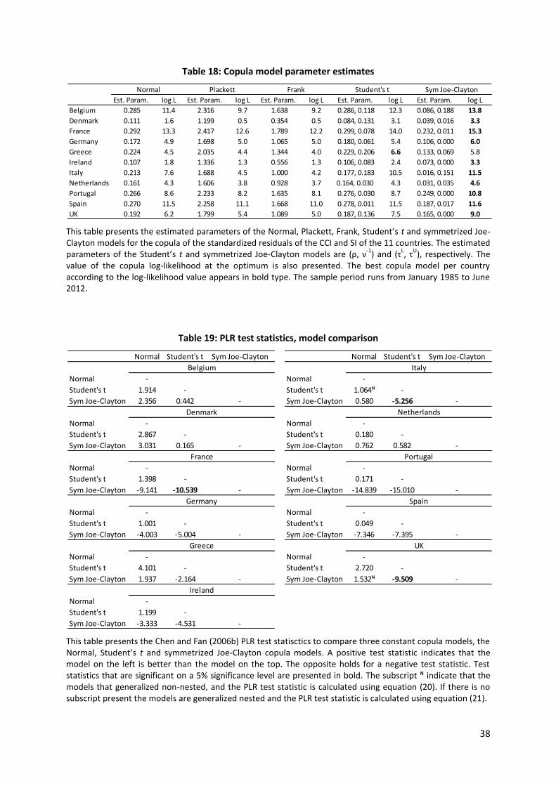
Table 18 presents the estimated parameters of these copula models allong with the values of
the log-likelihood. The estimated parameters of the SJC model are the lower and upper tail
dependence estimates. Here the same conclusions are obtained as in Table 16. The lower and upper
tail dependies do not differ significantly from each other with a 5% significance level. Although not
significant, there are some differences between lower and upper tail dependencies seen. For most of
the countries the lower tail dependence is larger, except for Belgium and Italy, which indicates that in
lesser times the CCI and the stock market move closer together than in better times. These results
are in line with the contemporaneous bull/bear market and threshold correlation results.
According to the log-likelihood values in Table 18, the SJC model is the best copula model for
most of the countries, except for Greece where the Student’s t model is the best copula model fit.
The SJC model as the best fit for most of the countries is followed by the Student’s t and the Normal
copula. To analyze if the SJC model is significantly a better fit for the data than the Normal and
Student’s t models I use the pseudo –likelihood ratio (PLR) test described by Chen and Fan (2006b).
This test is constructed for model selection between two semiparametric copula-based models. Chen
and Fan (2006b) show that for models that are generalized non-nested9 the likelihood ratio t test
statistic can be written as:
NT =
T
TTTT LLT
ˆ
ˆˆ2211
2/1 (20)
where
T
t
n
j
TjtTjttT QQdT 1
2
1
1122
2 )ˆ(ˆ)ˆ(ˆ~1ˆ
TtTtt UcUcd 2211ˆ;ˆlogˆ;ˆlog
Ttt ddd ~
T
tss
jsjsjt
j
iTsi
iTijt UUUu
Uc
TQ
,1
ˆˆˆ1)ˆ;ˆ(log1
)ˆ(ˆ
9
Chen and Fan (2006b) state that two models are generalized non-nested if the set
*
212
*
1111 ;,...,;,...,:,..., ddd uucuucuu has positive Lebesgue measure (the volume measure),
with α* the pseudo true value. They test the null hypothesis of generalized nested models by testing H0:
02 a . The estimator of 2
a is given by
T
t
ta dT 1
22 ~1
.
37
where the subscript N in NT is meant for non-nested models. This test statistic is Normally
distributed under the null hypothesis that the benchmark copula model is not worse than the
candidate copula model. The test is derived under the assumption that the conditional copula is
constant.
When two models are generalized nested, the test statistic is defined as:
QT = TTTT LLT 2211ˆˆ2 (21)
where the subscript Q in QT is meant for non-nested models. This PLR test statistic has a distribution
of a weighted sum of independent 2
)1( random variables, the weight is the 1)( 21 aa vector of
eigenvalues of the matrix W defined as
1
11
1
212
1
1
'
12
1
22
BB
BBW .
Table 19 presents the results of the PLR test described above. The results show that most of
the test statistics are not significant. Only for France, Italy and the UK there can be stated that the
Student’s t model significantly beats the SJC model. Furthermore, there can be seen that the
Student’s t model is always prefered over the Normal model, but not significantly. And for 8 (3 of
them are significant) out of the 11 countries the Student’s t model is also prefered over the SJC
model. Table 19 also shows that only in two cases the compared models are considered generalized
non-nested, resulting from the Chen and Fan (2006b) test on the null hypothesis that the two models
are generalized nested. The reason that not much of the differences in likelihood values in Table 18
are confirmed by the PLR test results and that most of the models are considered generalized nested
could be that the three models that are analyzed are quite similar for the central region and the
small number of observation. The largest differences between these models occur in the tails, where
we have less data to distinguish between the competing specifications. Concluding, it is not really
clear which copula model would be the best to model the dependence between the CCI and the
stock market.
38
Table 18: Copula model parameter estimates
This table presents the estimated parameters of the Normal, Plackett, Frank, Student’s t and symmetrized Joe-Clayton models for the copula of the standardized residuals of the CCI and SI of the 11 countries. The estimated parameters of the Student’s t and symmetrized Joe-Clayton models are (ρ, ν
-1) and (τ
L, τ
U), respectively. The
value of the copula log-likelihood at the optimum is also presented. The best copula model per country according to the log-likelihood value appears in bold type. The sample period runs from January 1985 to June 2012.
Table 19: PLR test statistics, model comparison
This table presents the Chen and Fan (2006b) PLR test statisctics to compare three constant copula models, the Normal, Student’s t and symmetrized Joe-Clayton copula models. A positive test statistic indicates that the model on the left is better than the model on the top. The opposite holds for a negative test statistic. Test statistics that are significant on a 5% significance level are presented in bold. The subscript ᴺ indicate that the models that generalized non-nested, and the PLR test statistic is calculated using equation (20). If there is no subscript present the models are generalized nested and the PLR test statistic is calculated using equation (21).
Est. Param. log L Est. Param. log L Est. Param. log L Est. Param. log L Est. Param. log L
Fisher, Kenneth L., and Meir Statman, 2003, Consumer confidence and stock returns, Journal of
Portfolio Management, 30:1, 115-127.
Frahm, Gabriel, Markus Junker and Rafael Schmidt, 2005, Estimating the tail-dependence coefficient: Properties and pitfalls, Insurance: Mathematics and Economics, 37, 80-100.
42
Franses, Philip H., and Dick van Dijk, 2007, Time series models for business and econometric
forecasting, Prepared for Cambridge University Press.
Granger, Clive W.J., 1980, Testing for causality: a personal viewpoint, Journal of Economic Dynamics
and Control 2, 329-352.
Guiso, Luigi, Michael Haliassos and Tullio Jappelli, 2003, Household stockholding in Europe: Where do
we stand and where do we go?, Economic Policy, 18:36, 123-170.
Howrey, E. Philip, 2001, The predictive power of the index of consumer sentiment, Brookings Papers
on Economic Activity, 2001:1, 175-207.
Hu, Ling, 2006, Dependence patterns across financial markets: a mixed copula approach, Applied
Financial Economics, 16:10, 717-729.
Jansen, W. Jos, and Niek J. Nahuis, 2003, The stock market and consumer confidence: European
evidence, Economics Letters 79, 89-98.
Joe, Harry, 1997, Multivariate Models and Dependence Concepts, Chapman and Hall, London. ISBN 0-
412-07331-5.
Kim, Seung-Nyeon, and Wankeun Oh, 2009, Relationship between consumer sentiment and stock
price in Korea, The journal of the Korean Economy, 10:3, December, 421-442.
Kole, Erik, and Dick van Dijk, 2010, How to identify and predict bull and bear markets?, September.
Liu, Lily, Andrew J. Patton and Kevin Sheppard, 2012, Does anything beat 5-minute RV? A comparison
of realized measures across multiple asset classes, May.
Ludvigson, Sydney C., 2004, Consumer confidence and consumer spending, The journal of Economic
Perspectives, 18:2, 29-50.
Lunde, Asger and Allan Timmermann, 2004, Duration dependence in stock prices: An analysis of
bull and bear markets, Journal of Business & Economic Statistics, 22:3, 253–273.
43
Lüutkepohl, Helmut, Pentti Saikkonen and Carsten Trenkler, 2001, Maximum eigenvalue versus trace
tests for the cointegration rank of a VAR process, The Econometrics Journal, 4:2, December, 287-310.
Matsusaka, John G., and Argia M. Sbordone, 1995, Consumer confidence and economic fluctuations,
Economic Inquiry, 33, April, 296-318.
Nelsen, Roger B., 1999, An Introduction to Copulas, New York Springer Series. ISBN 978-0-387-98623-
4.
NU.nl, Het consumentenvertrouwen is cruciaal, September 17, 2011. March 27, 2012,
Oh, Dong H., and Andrew J. Patton, 2012, Modelling dependence in high dimensions with factor
copulas, April.
Otoo, Maria W., 1999, Consumer sentiment and the stock market, Finance and Economics Discussion
Paper 60, November (Federal Reserve Board, Washington D.C.).
Patton, Andrew J., 2006, Modelling asymmetric exchange rate dependence, International Economic
Review, 47:2, 527-556.
Patton, Andrew J., 2012, Copula methods for forecasting multivariate time series, Handbook of
Economic Forecasting Volume 2, forthcoming.
Patton, Andrew J., 2012, A Review of Copula Models for Economic Time Series, Journal of Mul-
tivariate Analysis, 110, April, 4-18.
Sklar, A., 1959, Fonctions de répartition à n dimensions et leurs marges, Publications de l’Institut de
Statistique de l’Université de Paris pp. 229–231.
44
Appendix
Table A.1: ADF and Phillip-Perron test
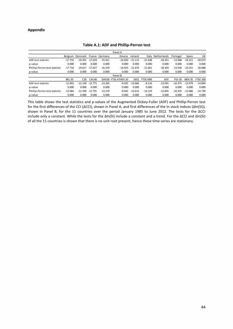
This table shows the test statistics and p-values of the Augmented Dickey-Fuller (ADF) and Phillip-Perron test for the first differences of the CCI (ΔCCI), shown in Panel A, and first differences of the ln stock indices (Δln(SI)), shown in Panel B, for the 11 countries over the period January 1985 to June 2012. The tests for the ΔCCI include only a constant. While the tests for the Δln(SI) include a constant and a trend. For the ΔCCI and Δln(SI) of all the 11 countries is shown that there is no unit root present, hence these time series are stationary.
Belgium Denmark France Germany Greece Ireland Italy Netherlands Portugal Spain UK
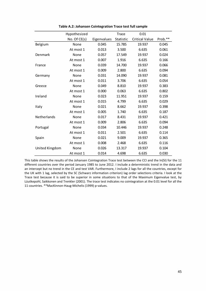
Table A.2: Johansen Cointegration Trace test full sample
This table shows the results of the Johansen Cointegration Trace test between the CCI and the ln(SI) for the 11 different countries over the period January 1985 to June 2012. I include a deterministic trend in the data and an intercept but no trend in the CE and test VAR. Furthermore, I include 2 lags for all the countries, except for the UK with 1 lag, selected by the SC (Schwarz information criterion) lag order selections criteria. I look at the Trace test because it is said to be superior in some situations to that of the Maximum Eigenvalue test, by Lüutkepohl, Saikkonen and Trenkler (2001). The trace test indicates no cointegration at the 0.01 level for all the 11 countries. **MacKinnon-Haug-Michelis (1999) p-values.
Hypothesized Trace 0.01
No. Of CE(s) Eigenvalues Statistic Critical Value Prob.**
Belgium None 0.045 15.785 19.937 0.045
At most 1 0.013 3.500 6.635 0.061
Denmark None 0.057 17.549 19.937 0.024
At most 1 0.007 1.916 6.635 0.166
France None 0.039 14.700 19.937 0.066
At most 1 0.009 2.800 6.635 0.094
Germany None 0.031 14.090 19.937 0.081
At most 1 0.011 3.706 6.635 0.054
Greece None 0.049 8.810 19.937 0.383
At most 1 0.000 0.063 6.635 0.802
Ireland None 0.023 11.951 19.937 0.159
At most 1 0.015 4.799 6.635 0.029
Italy None 0.021 8.662 19.937 0.398
At most 1 0.005 1.740 6.635 0.187
Netherlands None 0.017 8.431 19.937 0.421
At most 1 0.009 2.806 6.635 0.094
Portugal None 0.034 10.446 19.937 0.248
At most 1 0.011 2.501 6.635 0.114
Spain None 0.021 9.009 19.937 0.365
At most 1 0.008 2.468 6.635 0.116
United Kingdom None 0.026 13.317 19.937 0.104
At most 1 0.014 4.698 6.635 0.030
46
Table A.3: Granger causality full sample
This table presents the p-values of the Granger causality test for the full sample in two directions, from the CCI to the stock indices and from the stock indices to the CCI, with lags k = 1,3,6. The sample period runs from January 1985 to June 2012.
CCI to SI SI to CCI CCI to SI SI to CCI CCI to SI SI to CCI
Belgium 0.615 0.003 0.478 0.026 0.418 0.022
Denmark 0.458 0.017 0.338 0.037 0.600 0.022
France 0.171 0.002 0.579 0.019 0.897 0.004
Germany 0.839 0.020 0.492 0.003 0.580 0.012
Greece 0.984 0.070 0.963 0.133 0.750 0.092
Ireland 0.364 0.000 0.904 0.000 0.560 0.000
Italy 0.656 0.000 0.918 0.001 0.069 0.015
Netherlands 0.995 0.000 0.620 0.000 0.478 0.000
Portugal 0.407 0.206 0.369 0.138 0.488 0.168
Spain 0.335 0.002 0.438 0.005 0.749 0.041
UK 0.727 0.001 0.357 0.005 0.792 0.012
k=1 k=3
Granger causality (p-values)
k=6
47
Table A.4: Johansen Cointegration Trace test 1985-1998
This table shows the results of the Johansen Cointegration Trace test between the CCI and the ln(SI) for the 11 different countries over the period January 1985 to December 1998. I include a deterministic trend in the data and an intercept but no trend in the CE and test VAR. Furthermore, I include 2 lags for all the countries, except for the UK with 1 lag, selected by the SC (Schwarz information criterion) lag order selections criteria. I look at the Trace test because it is said to be superior in some situations to that of the Maximum Eigenvalue test, by Lüutkepohl, Saikkonen and Trenkler (2001). The trace test indicates no cointegration at the 0.01 level for all the countries, exception being Greece. **MacKinnon-Haug-Michelis (1999) p-values.
Hypothesized Trace 0.01
No. Of CE(s) Eigenvalues Statistic Critical Value Prob.**
Belgium None 0.113 12.637 19.937 0.129
At most 1 0.000 0.001 6.635 0.974
Denmark None 0.054 6.600 19.937 0.625
At most 1 0.007 0.749 6.635 0.387
France None 0.034 4.965 19.937 0.813
At most 1 0.002 0.331 6.635 0.565
Germany None 0.025 6.684 19.937 0.615
At most 1 0.015 2.442 6.635 0.118
Greece None 0.773 22.788 19.937 0.003
At most 1 0.238 3.540 6.635 0.060
Ireland None 0.068 11.814 19.937 0.166
At most 1 0.002 0.266 6.635 0.606
Italy None 0.041 10.691 19.937 0.231
At most 1 0.023 3.822 6.635 0.051
Netherlands None 0.027 4.733 19.937 0.837
At most 1 0.002 0.279 6.635 0.597
Portugal None 0.078 5.830 19.937 0.716
At most 1 0.002 0.167 6.635 0.683
Spain None 0.037 5.285 19.937 0.778
At most 1 0.000 0.003 6.635 0.955
United Kingdom None 0.033 5.847 19.937 0.714
At most 1 0.002 0.316 6.635 0.574
48
Table A.5: Johansen Cointegration Trace test 1999-2012
This table shows the results of the Johansen Cointegration Trace test between the CCI and the ln(SI) for the 11 different countries over the period January 1985 to June 2012. I include a deterministic trend in the data and an intercept but no trend in the CE and test VAR. Furthermore, I include 2 lags for all the countries, except for the UK with 1 lag, selected by the SC (Schwarz information criterion) lag order selections criteria. I look at the Trace test because it is said to be superior in some situations to that of the Maximum Eigenvalue test, by Lüutkepohl, Saikkonen and Trenkler (2001). The trace test indicates no cointegration at the 0.01 level for all the 11 countries. **MacKinnon-Haug-Michelis (1999) p-values.
Hypothesized Trace 0.01
No. Of CE(s) Eigenvalues Statistic Critical Value Prob.**
Belgium None 0.038 8.627 19.937 0.401
At most 1 0.015 2.387 6.635 0.122
Denmark None 0.075 18.364 19.937 0.018
At most 1 0.035 5.768 6.635 0.016
France None 0.091 18.565 19.937 0.017
At most 1 0.019 3.060 6.635 0.080
Germany None 0.049 12.840 19.937 0.121
At most 1 0.028 4.649 6.635 0.031
Greece None 0.034 5.593 19.937 0.743
At most 1 0.000 0.006 6.635 0.940
Ireland None 0.028 6.067 19.937 0.688
At most 1 0.012 1.819 6.635 0.177
Italy None 0.022 3.582 19.937 0.934
At most 1 0.000 0.036 6.635 0.850
Netherlands None 0.063 12.646 19.937 0.128
At most 1 0.013 2.041 6.635 0.153
Portugal None 0.025 5.497 19.937 0.754
At most 1 0.009 1.476 6.635 0.225
Spain None 0.045 9.725 19.937 0.303
At most 1 0.014 2.207 6.635 0.137
United Kingdom None 0.036 8.599 19.937 0.404
At most 1 0.016 2.604 6.635 0.107
49
Table A.6: Dynamic correlations two periods, 1985-1998 1999-2012
This table presents the dynamic correlation estimates of the consumer confidence, CCI(t), and the associated stock market, SI(t-j), of the 11 countries, for j = -1,…,1. The superscripts (***), (**) and (*) indicate statistical significance at a 1%, 5% and 10% level respectively. Columns 1-3 show the correlation estimates for the sample period January 1985 until December 1998. Columns 4-6 show the correlation estimates for the sample period January 1999 until June 2012.
Figure A.1: Identification of bull and bear markets
51
This figure shows the identification of bull and bear market periods for the different countries over the period January 1985 to June 2012. Some countries have a shorter sample period, depending on the CCI and SI data that is available, which is presented in the Data section. The algorithm that is used to identify the bull and bear markets is the Lunde and Timmerman (2004) algorithm. The thin black line plots the stock market index, and the thick black line plots the CCI. Purple areas indicate bear markets, and white areas correspond with bull markets.
52
Table A.7: VAR models bull market
This table shows the VAR model results presented in (5) and (6) for the sample running from January 1985 to June 2012 for when the state of the economy is considered to be a bull market. The number of lags used are different per country depending on the outcome of the Portmanteau test, see table 6. Standard errors are presented in parentheses.
This table shows the VAR model results presented in (5) and (6) for the sample running from January 1985 to June 2012 for when the state of the economy is considered to be a bear market. The number of lags used are different per country depending on the outcome of the Portmanteau test, see table 6. Standard errors are presented in parentheses.
This figure shows the quantile dependence results for the different countries. The left panel presents the estimated quantile dependence between the residuals for the CCI and the SI, along with a 90% bootstrap confidence interval. The right panel presents the difference between the corresponding upper and lower quantile along with 90% bootstrap confidence interval for this difference. The sample period runs from January 1985 to June 2012.