THE RIEMANN-ROCH THEOREM AND SERRE DUALITY JOHN HALLIDAY Abstract. We introduce sheaves and sheaf cohomology and use them to prove the Riemann-Roch theorem and Serre duality. The main proofs follow the treatment in Forster [3]. Contents 1. Introduction 1 2. Sheaves 2 3. Sheaf Cohomology 3 4. Exact Sequences of Sheaves 5 5. De Rham Cohomology 7 5.1. A Few Exact Sequences 7 5.2. The De Rham Groups and a Special Case of Serre Duality 8 6. Genus 9 7. The Riemann-Roch Theorem 9 8. Serre Duality 13 8.1. Residue as a Linear Functional on H 1 (O) 13 8.2. The Proof of Serre Duality 15 9. Applications 18 9.1. the Degree of K and the Riemann-Hurwitz Formula 18 9.2. Applications to Riemann Surfaces 20 10. Conclusion 21 11. Acknowledgments 21 References 22 1. Introduction The theory of Riemann surfaces lies at the crossroads of algebra and geome- try. A compact Riemann surface has two characterizations, both as a compact complex 1-manifold and as a nonsingular algebraic curve. The function field of a Riemann surface, the set of all meromorphic functions defined on it, has a geomet- ric interpretation as the set of maps from the curve to the Riemann sphere. The Riemann-Roch theorem is a statement about the dimension of certain subsets of the function field, subsets where we have required that poles may only occur at certain locations, and that their poles must not be too high a negative degree. The Riemann-Roch theorem is a bridge from the genus, a characteristic of a surface as a topological space, to algebraic information about its function field. A more Date : August 28, 2015. 1
Transcript
THE RIEMANN-ROCH THEOREM AND SERRE DUALITY
JOHN HALLIDAY
Abstract. We introduce sheaves and sheaf cohomology and use them to prove
the Riemann-Roch theorem and Serre duality. The main proofs follow the
treatment in Forster [3].
Contents
1. Introduction 12. Sheaves 23. Sheaf Cohomology 34. Exact Sequences of Sheaves 55. De Rham Cohomology 75.1. A Few Exact Sequences 75.2. The De Rham Groups and a Special Case of Serre Duality 86. Genus 97. The Riemann-Roch Theorem 98. Serre Duality 138.1. Residue as a Linear Functional on H1(O) 138.2. The Proof of Serre Duality 159. Applications 189.1. the Degree of K and the Riemann-Hurwitz Formula 189.2. Applications to Riemann Surfaces 2010. Conclusion 2111. Acknowledgments 21References 22
1. Introduction
The theory of Riemann surfaces lies at the crossroads of algebra and geome-try. A compact Riemann surface has two characterizations, both as a compactcomplex 1-manifold and as a nonsingular algebraic curve. The function field of aRiemann surface, the set of all meromorphic functions defined on it, has a geomet-ric interpretation as the set of maps from the curve to the Riemann sphere. TheRiemann-Roch theorem is a statement about the dimension of certain subsets ofthe function field, subsets where we have required that poles may only occur atcertain locations, and that their poles must not be too high a negative degree. TheRiemann-Roch theorem is a bridge from the genus, a characteristic of a surfaceas a topological space, to algebraic information about its function field. A more
Date: August 28, 2015.
1
2 JOHN HALLIDAY
elementary treatment would build the Riemann-Roch theorem directly from singu-lar homology. Though this treatment is valuable, we use the language of sheavesand sheaf cohomology from the beginning. This method is more abstract, but themethods we use are very powerful and easily admit generalization. We attemptto give a comprehensive introduction to the machinery we utilize, and hopefullythe geometric intuition of more elementary methods is preserved. Familiarity withbasic Riemann surface theory and differential forms is assumed, but much of thepaper may be readable without it. Whenever we do not explicitly state the underly-ing space of a sheaf, it can be assumed to be a compact connected Riemann surface.
2. Sheaves
We begin by introducing sheaves. Speaking informally, a sheaf is an objectdefined on a topological space which can capture local data on any open set, butcan also give us information about the global structure of the object.
Definition 2.1. A presheaf 1 F of abelian groups on a topological space (X, T ) isa collection of abelian groups (F(U))U∈T along with a collection of group homo-morphisms ρUV whenever U, V are open and V ⊂ U , such thati) ρUW = ρVW ρUV .ii) ρUU = IdU .
In this paper, these groups will always be groups of functions, so a presheaf is a setof functions on each open set in X, with ρUV the typical restriction map of functionson U to functions on V. We thus use the typical notation f|V = ρUV f .
Definition 2.2. A sheaf of abelian groups is a presheaf of abelian groups suchthati) Given a collection (Ui)i∈I of open sets with U =
⋃i∈I Ui, and elements fi ∈
F(Ui), if fi|Ui∩Uj= fj |Ui∩Uj
for all i, j ∈ I, there exists f ∈ F(U) such that
f|Ui= fi for all i ∈ I.
ii) if f, g ∈ F(U) and f|Ui= g|Ui
for all i ∈ I, then f = g.
A sheaf lets us patch functions that agree on the overlap of their domains into aunique larger function.
Examples 2.3. Examples of sheaves on a Riemann surface:O : The sheaf of holomorphic functions.Ω : The sheaf of holomorphic 1-forms.C : The sheaf of locally constant functions with values in C.E : The sheaf of differentiable functions.E(1) : The sheaf of differentiable 1-forms.E1,0 : The sheaf of differentiable 1-forms which locally look likefdz, aka have no dz term.Z : The sheaf of closed 1-forms.
We now want to define the stalk at a sheaf. speaking very nonrigorously, we wantto take a single point x ∈ X and see how much information in the sheaf can beseen from the vantage point of x. The stalk should tell us what the sheaf looks like
1In other words, a presheaf is a contravariant functor from the category with open sets in Xas objects and inclusion maps as morphisms to the category of abelian groups.
THE RIEMANN-ROCH THEOREM AND SERRE DUALITY 3
locally around x. To translate this statement into mathematical rigor, we just takethe direct limit over all neighborhoods of x.
Definition 2.4. The stalk of F at x, denoted Fx is defined as Fx = lim−→U3x F(U).
Some facts which follow simply from the definition of direct limits are relevant. Forinstance, if [f, x] = [g, x], where f ∈ F(U1), g ∈ F(U2), and [f, x] and [g, x] are theircorresponding elements in Fx, then there exists a neighborhood of x V ⊂ U1 ∩ U2
such that f|V = g|V . Looking at stalks allows us to discuss the local properties ofsheaves in greater rigor. For instance, when we define exact sequences of sheaves,we will say that a sequence of sheaves is exact when it is ”locally exact” whichmeans the corresponding sequence of stalks at a point x is exact for every x ∈ X.
3. Sheaf Cohomology
Sheafs are fundamentally a local-to-global object, something that takes localinformation and builds it into a global structure. Along those same lines, we firstdefine sheaf cohomology as relative to an open cover, then take the direct limit overall possible open covers.
Definition 3.1. given an open cover U = (Ui)i∈I and a sheaf F , We define thezeroth cochain group C0(U ,F) =
∏i∈I F(Ui). The zeroth cochain group is a
collection of local sections of the sheaf F . An element of C0(U ,F) is denoted(fi)i∈I .
Definition 3.2. With U ,F as above, for any natural number q we define the q-thcochain group Cq(U ,F) =
∏i0,...iq∈I F(Ui0 ∩ · · · ∩Uiq ). An element of Cq(U ,F) is
denoted (fi0,...iq )i0,...iq∈I .
In particular, the first cochain group C1(U ,F) =∏i,j∈I F(Ui ∩ Uj).
From the point of view of cohomology theory, it is natural that we define a cobound-ary operator. It is easy to see how an element of C0 maps to an element of C1 byrestricting the two functions fi and fj to Ui ∩ Uj and subtracting them. For ourpurposes we only need define its actions on C0 and C1, but the definition extendsin the obvious way to δ :
⋃∞i=0 C
i(U ,F)→⋃∞i=1 C
i(U ,F). The operator takes anyelement of Ci(U ,F) to Ci+1(U ,F).
Definition 3.3. We define δ : C0(U ,F)→ C1(U ,F):δ(fi) = (gi,j), where gi,j = fj |Ui∩Uj
− fi|Ui∩Uj.
We define δ : C1(U ,F)→ C2(U ,F):δ(fi,j) = (gi,j,k), where gi,j,k = fi,j |Ui∩Uj∩Uk
+ fj,k|Ui∩Uj∩Uk+ fk,i|Ui∩Uj∩Uk
.
Intuitively, the boundary operator on C0 measures the failure of a 0-cochain to pastetogether into a global section. If δ(f) = 0, then fi|Ui∩Uj
= fj |Ui∩Ujfor all i, j ∈ I,
so by the first sheaf axiom we can paste (fi) together into a function f ∈ F(X). El-ements in C0 as above are called closed cochains, and the group of closed 0-cochainsis denoted Z0(U ,F). Clearly Z0(U ,F) = ker(δ) ∩ C0(U ,F). Similarly, we defineZ1(U ,F) = ker(δ)∩C1(U ,F). In other words, Z1(U ,F) = (fi,j)i,j∈I : δ(fi,j) = 0.
4 JOHN HALLIDAY
We define the coboundary set B1(U ,F) = Im(δ) ∩C1(U ,F) = (fi,j) ∈ C1(U ,F) :∃(gi) ∈ C0(U ,F)such thatfi,j = gj |Ui∩Uj
− gi|Ui∩Uj We define B0(U ,F) = 0.
It is clear that δ δ = 0. Consider δ δ(f) = δ(fj − fi)i,j∈I = (fj − fi + fk − fj +fi − fk)i,j,k∈I = 0. This means that B1(U ,F) ⊂ Z1(U ,F). what we wish to dowith these groups is measure the failure of a closed cochain to be a coboundary; inother words, the failure of δ to be exact as a cochain operator.
Definition 3.4. We define the ith cohomology groupHi(U ,F) = Zi(U ,F)/Bi(U ,F)
Since B0(U ,F) = 0, H0(U ,F) − Z0(U ,F). As we saw before H0 is the set ofglobal sections of the sheaf F . A lot of what we do next is devoted to developingan understanding of the first cohomology group H1(F). However, our definition ofcohomology is still dependent on a specific open cover.
Definition 3.5. given two open covers B = (Bk)k∈K and U = (Ui)i∈I , we say Bis finer than U , denoted B < U , if for all Bk ∈ B, there exists Uτi ∈ U such thatBk ⊂ Uτk, where τ is a map from K to I.
In other words, every set in B must be contained in a set in U .
This is the natural restriction mapping of cochains induced by our map τ . SinceτUB clearly maps B1(U ,F) to B1(B,F), it factors through to a map from H1(U ,F)to H1(B,F).We omit proofs of the following two lemmas, which are tedious.
Lemma 3.7. The map τUB : H1(U ,F)→ H1(B,F) doesn’t depend on the choice ofthe map τ .
Lemma 3.8. The map τUB : H1(U ,F)→ H1(B,F) is injective.
With those two facts, we can define H1(X,F) = lim−→H1(U ,F) where the direct
limit is taken over all open covers of X. Because all the maps τUB are injective, weknow that every H1(U ,F) injects into H1(X,F), so the first sheaf cohomology ofa space is at least as large as the cohomology relative to any of its open covers. Wewill usually just write H1(F) instead of H1(X,F).
Theorem 3.9. H1(E) = 0.
Proof. This fact relies on the idea of partitions of unity. We use the fact that forany open cover U = (Ui)i∈I , there exists a set of functions (ψi)i∈I such thati) supp(ψi) ⊂ Uiii) for any x ∈ X, there is a neighborhood Vx so Vx only interesects finitely manysupp(ψi)ii)∑i∈I ψi(x) = 1 for all x ∈ X.
Knowing this, we consider (fij) ⊂ Z1(U , E). Now we want to find gi so gi−gj = fijon Ui ∩ Uj . We set gi =
∑k∈I ψkfik. This can be defined as a differentiable
element of E(Ui) since each function ψifij can be seen as zero outside of supp(ψi),
THE RIEMANN-ROCH THEOREM AND SERRE DUALITY 5
and because the sum is differentiable since all of its terms are and it is locally finite.Now, we have
gi − gj =∑k∈I
ψk[fik − fjk]
=∑k∈I
ψkfij
= fij
A near-identical version of this proof shows that E1,0, E0,1, E(1), and E(2) all havetrivial first cohomology.
4. Exact Sequences of Sheaves
Much of the reason sheaf cohomology is interesting is because of how it relatesto exact sequences of sheaves. To define an exact sequence of sheaves, we must firstdefine a sheaf homomorphism.
Definition 4.1. a sheaf homomorphism α : F → G is a collection of maps αU :F(U) → G(U) such that the maps commute with restriction maps, meaning thatfor all open sets U , V so V ⊂ U ,
F(U)αU //
ρUV
G(U)
ρUV
F(V )αV
// G(V )
where the restriction maps of F are represented by ρ and the restriction maps ofG are represented by ρ.
This map induces homomorphisms of stalks Fxαx−−→ Gx. We define the map to
be a monormprhism of sheaves if it is a monomorphism on each stalk, and anepimorphism of sheaves if it is an epimorphism on each stalk. We define an exact
sequence of sheaves F α−→ G β−→ H to be exact if for all x ∈ X, the sequence
Fxαx−−→ Gx
βx−→ Hx
is exact. A short exact sequence 0→ F α−→ G β−→ H → 0 is then exact if it inducesa short exact sequence on stalks. We are interested in how this definition of exactsequences interacts with the induced maps on cohomology. The simplest exampleof this is just the maps induced on the zeroth cohomology groups, aka the globalsections of X. Before we study that, however, we prove more general facts aboutthe induced maps F(U)→ G(U)→ H(U).
Lemma 4.2. suppose α : F → G is a sheaf monomorphism. Then every mapαU : F(U)→ G(U) is a monomorphism.
Proof. since α is a sheaf monomorphism, αx is injective for all x ∈ X supposeαU (f) = 0. Then for all x ∈ U , αx([f, x]) = 0. Thus, [f, x] = [0, x] for all x ∈ U .Thus, around each x there exists an open neighborhood Vx 3 x so that f|Vx
= 0.By sheaf axiom II, f = 0 on U .
6 JOHN HALLIDAY
This lemma tells us that going from a sheaf homomorphism to a homomorphismof local sections preserves injectivity. However, it does not preserve surjectivity, aswe can easily see from looking at the exponential map on C.
O exp−−−→ O∗
where exp(f) = e2πif . That this is locally but not globally surjective is funda-mentally a restatement about properties of the logarithm from complex analysis.We know around any point there is a simply connected neighborhood of the pointcontained in C∗ within which exp is invertible. But on some non-simply connectedneighborhoods, in particular C∗ itself, the logarithm is not gloablly defined, so thefunction Id ∈ O∗(C∗) has no preimage under exp.
This example tells us that we cannot always get a short exact sequence of sectionsfrom a short exact sequence of sheaves, but as our next theorem shows we can atleast preserve part of the exactness.
Theorem 4.3. If 0→ F α−→ G β−→ H is an exact sequence of sheaves, then for anyopen set U ,
0→ F(U)α−→ G(U)
β−→ H(U)
is exact. 2
Proof. (i) That α is injective we proved in theorem 4.3.
(ii) Im(α) ⊂ Ker(β): Consider f ∈ F(U), g = α(f) ∈ G(U). On any stalk Gx,[g, x] = αx[f, x], so βx[g, x] = [0, x]. by basic properties of the direct limit, thismeans that on some open set Vx about x, β(g|Vi) = 0. By Sheaf axiom I, theseβ(g|Vi) paste together into a global function 0, so β(g) = 0.
(iii) Ker(β) ⊂ Im(α). This is pretty much the same idea as (ii). considerg ∈ G(U) so β(g) = 0. Then on any stalk [g, x] = αx[fx, x], and so g|Vx = α(fx) forsome neighorhood Vx 3 x and fx ∈ F(Vx). This is an open cover, and α(fx|Vx∩Vy
) =
α(fy |Vx∩Vy) = g|Vx∩Vy
. Since α is injective, this means fx|Vx∩Vy) = fy |Vx∩Vy
, so
they can be pasted together into a global function f ∈ F(U) so that α(f) = g
We are most interested in this lemma when the original sequence is actually ashort-exact sequence, meaning β is surjective, and when U = X. We then have
that 0 → H0(F)α0−→ H0(G)
β0−→ H0(H). The amazing fact is that this sequenceextends to a long exact sequence on cohomology, namely that in a canonical way
we can attach the sequence H1(F)α1−→ H1(G)
β1−→ H1(H) to the end of this one.
Definition 4.4. if we have 0→ F α−→ G β−→ H → 0, then we define the connectinghomomorphism δ∗ : H0(H) → H1(F) as follows: We consider h ∈ H0(H). sinceβ is surjective on stalks, we proceed as in Theorem 4.3 (part iii of the proof) andconstruct an open cover V = (Vx), and a corresponding cochain g = (gx) ∈ C0(V,G)so that β(g) = h|Vx
. But since β(gx−gy) = 0 on Vx∩Vy, we apply theorem 4.3 withU = Vx ∩ Vy and get an element f = (fxy) ∈ F(Vx ∩ Vy) so that α(fxy) = gx − gy.Doing this for all pairs (x, y) gets us a cochain (fij) ∈ C1(V,F). Clearly (fij)
2In other words, the functor taking a sheaf on a space to its group on an open set is left-exact.
THE RIEMANN-ROCH THEOREM AND SERRE DUALITY 7
is closed. We denote δ∗h = [fxy], where [fxy] is the cohomology class of (fxy) inH1(F).
That δ∗ is well-defined is tedious but simple to check. Finally, we have reached themost important theorem of this section:
Theorem 4.5. With 0→ F α−→ G β−→ H → 0, δ∗ as above, The sequence
0 // H0(F)α0 // H0(G)
β0 // H0(H)δ∗ //
. . . // H1(F)α1 // H1(G)
β1 // H1(H)
is exact.
The proof of this theorem is long but doesn’t involve any original ideas, so weomit it.3. This theorem is important because it allows us to get information aboutH1 groups, and write them in terms of quotients of H0 groups, giving a concreteinterpretation to H1 groups.
Corollary 4.6. If 0 → F α−→ G β−→ H → 0 is exact, and H1(G) = 0, we haveH1(F) = H0(H)/βH0(G).
Proof. We have the long exact sequence
0→ H0(F)α−→ H0(G)
β−→ H0(H)→ H1(F)→ 0.
We will use this technique several times in the next section.
5. De Rham Cohomology
5.1. A Few Exact Sequences. We consider a few exact sequences of sheaves.First, we define two operators:
Definition 5.1. We know that d(f) = fzdz + fzdz. We define ∂f = fzdz, and∂f = fzdz. This definition on functions extends to forms in the same way thenormal definition of the differential does. Where d maps Ep,q to Ep+1,q ⊕ Ep,q+1, ∂maps Ep,q to Ep+1,q and ∂ maps Ep,q to Ep,q+1. Clearly we have d = ∂ + ∂.
A function is holomorphic if ∂f = 0, for example.
Theorem 5.2. The following sequences are exact.
0→ C→ E d−→ Z → 0
0→ C→ O d−→ Ω→ 0
0→ O → E ∂−→ E0,1 → 0
0→ Ω→ E1,0 ∂−→ E(2) → 0
Proof. In the first sequence, since closed forms are locally exact, on any stalk, aclosed 1-form will be locally the differential of some function. The other sequencesare easy to check.
3The complete proof can be found in chapter 15 of [3].
8 JOHN HALLIDAY
5.2. The De Rham Groups and a Special Case of Serre Duality.
Definition 5.3. We define the de Rham cohomology groupH1DR(X) = H0(Z)/dH0(E).
The de Rham cohomology is the quotient of closed forms over exact forms. Thehigher de Rham groups are defined analogously, but we will have no need for them.
Theorem 5.4. De Rham’s Theorem for sheaves: H1DR(X) = H1(C).
Proof. Since we have the exact sequence 0 → C → E d−→ Z → 0, this extendsto a long-exact sequence on cohomology. Since H1(E) = 0, we have the sequence0→ C→ H0(E)→ H0(Z)→ H1(C)→ 0 is exact, and the proof follows.
We now want to show H0(Ω) = H1(O)∗. This is extremely important, not onlybecause it is a special case of Serre duality, but because it allows us to discuss theidea of a genus in a surface in a coherent way. Our proof relies on a theorem fromanalysis which we don’t prove 4, but whose statement should be relatively intuitive.
Lemma 5.5. if X is a compact connected Riemann surface, ρ a 2-form on X, thenthere exists a function f such that ∂∂f = ρ if and only if
∫Xρ = 0.5
Since the sequence 0 → O → E ∂−→ E0,1 → 0 is exact, and H1(E) = 0, we haveH1(O) = E0,1/dE . In this manner we treat H1(O) as cosets of (0, 1) forms. Wetake the map σ : σ(α) = [α], where the brackets represents taking a form to itsequivalence class.
Lemma 5.6. σ is surjective.
Proof. We consider some coset [β]. Now, we want to pick some representativeβ′ = ∂f so that ∂β′ = 0. Since β′ locally looks like fdz, and ∂β′ = fzdzdz, if∂β′ = 0 then ∂β′ = 0, and so β′ is a holomorphic 1-form as desired. But, ∂β′ = 0is equivalent to ∂∂f = −∂β, and since by Stokes’ theorem the latter side has zerointegral, we can apply our lemma and find an f such that this is possible. Thus, σis surjective.
Theorem 5.7. H0(Ω) = H1(O)∗.
Proof. Still viewing H1(O) as cosets of (0, 1) forms, we define the bilinear mapB : H0(Ω)⊕H1(O)→ C: B(α, [β]) =
∫Xα∧β. Since
∫Xα∧∂f =
∫X∂(αf) = 0 by
Stokes’ theorem, this is a well-defined map. Now, we define 〈 , 〉 : H0(Ω)⊕H0(Ω)→C: 〈α, β〉 = B(α, σ(β)).
But if α = fdz locally, 〈α, α〉 =∫Xfdz ∧ fdz =
∫X|f |2dz ∧ dz, which is positive
if α is not identically 0. So, given an element α ∈ H0(Ω), it acts nontrivially onits image σα, so it is a nonzero element of its dual. Thus B establishes a dualpairing.
The above proof additionally proves that σ is in fact an isomorphism, since it takesnonzero elements to nonzero elements and is therefore injective. We now thereforehave an isomrophism H1(O) = H0(Ω). We now want to prove that the de Rhamcohomology is equal to the direct sum of these two groups.
4A complete proof can be found in Chapter 9 of [2].5The operator ∂∂ is locally the laplacian ∂∂f = 4(∆f)dzdz.
THE RIEMANN-ROCH THEOREM AND SERRE DUALITY 9
Theorem 5.8. H0(Ω)⊕H1(O) ∼= H1DR.
Proof. Since H1(O) = H0(Ω), we can view this as H0(Ω) ⊕H0(Ω) ∼= H1DR. Now,
we have the map Ψ(α, β) = [α+ β]. This is injective: suppose α+ β = df . locally,α = adz, a holomorphic, and β = bdz, b antiholomorphic. Thus we would need tohave a = fz, b = fz. But this would mean f was both holomorphic and antiholo-morphic, so f is constant and α = β = 0.
The inverse map can be defined like this: we consider any closed 1-form ω, whichlocally equals adz + bdz. We can split a = a′ + a′′, b = b′ + b′′. where a′, b′ areholomorphic, a′′, b′′ antiholomorphic. Then dω = a′′z − b′zdz ∧ dz. since this mustbe zero if ω is closed, necesarily a′′z = b′z, and a holomorphic and antiholomorphicfunction are only equal if they are the same constant, so a′′ = cz+d, b′ = cz+e. So,a′′dz+ b′dz is clearly exact, and the values of a′ and b′′ are uniquely determined bythe cohomology class of ω. Thus the map ω → (a′dz, b′′dz) (in local coordinates)is injective, and is also an inverse of the above map Ψ.
6. Genus
An important aspect of the theory of Riemann surfaces is the idea of genus.Heuristically, genus measures the number of holes in a surface. A sphere has genus0, a torus has genus 1, etc. Since any Riemann surface, ignoring the complex struc-ture, is equivalent to a torus with some number of handles, this is the definitionwe want to keep in our mind. Defining this rigorously, we get that on a Riemannsurface, (or orientable surface in general), the genus is half the dimension of thefirst singular cohomology group with respect to Z.6 We don’t define singular co-homology in this paper, but the fact that it corresponds to the ”number of holes”in this way is very intuitive. It is a theorem known as de Rham’s theorem whichstates that on a smooth manifold (such as a Riemann surface) the de Rham coho-mology and singular cohomology are equal in dimension. A reader familiar withCech cohomology will also know that the first Cech cohomology of the constantsheaf is equal to the singular cohomology. So can compute this topological idea ofgenus using the de Rham cohomology or cohomology of the constant sheaf.
The second definition is that of geometric genus, which is dimH0(Ω), the dimensionof the space of holomorphic 1-forms on the surface. The third is dimH1(O), the di-mension of the first cohomology group of the sheaf of holomorphic functions. By ourtheorems in the previous section, we have seen that these dimensions are all equal:dimH0(Ω) = dimH1(O) = 1
2 dimH1DR. One of the most important aspects of the
Riemann-Roch theorem is its ability to translate topological information about aRiemann surface, that is, its genus, into algebraic information about subgroups ofits function field.
7. The Riemann-Roch Theorem
The Riemann-Roch Theorem is stated in the language of divisors. A divisor on acompact Riemann surface is essentially a way of encoding information about zerosand poles of a collection of meromorphic functions or forms.
6For more on this, look at [1].
10 JOHN HALLIDAY
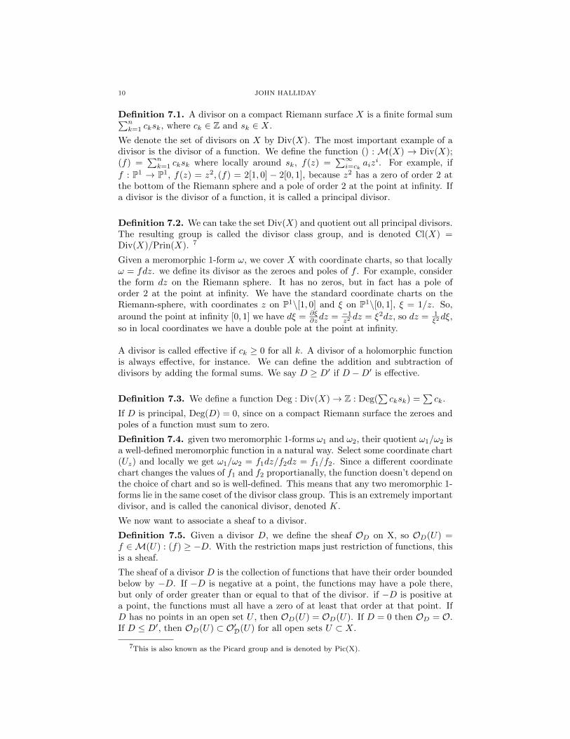
Definition 7.1. A divisor on a compact Riemann surface X is a finite formal sum∑nk=1 cksk, where ck ∈ Z and sk ∈ X.
We denote the set of divisors on X by Div(X). The most important example of adivisor is the divisor of a function. We define the function () : M(X) → Div(X);(f) =
∑nk=1 cksk where locally around sk, f(z) =
∑∞i=ck
aizi. For example, if
f : P1 → P1, f(z) = z2, (f) = 2[1, 0] − 2[0, 1], because z2 has a zero of order 2 atthe bottom of the Riemann sphere and a pole of order 2 at the point at infinity. Ifa divisor is the divisor of a function, it is called a principal divisor.
Definition 7.2. We can take the set Div(X) and quotient out all principal divisors.The resulting group is called the divisor class group, and is denoted Cl(X) =Div(X)/Prin(X). 7
Given a meromorphic 1-form ω, we cover X with coordinate charts, so that locallyω = fdz. we define its divisor as the zeroes and poles of f . For example, considerthe form dz on the Riemann sphere. It has no zeros, but in fact has a pole oforder 2 at the point at infinity. We have the standard coordinate charts on theRiemann-sphere, with coordinates z on P1\[1, 0] and ξ on P1\[0, 1], ξ = 1/z. So,
around the point at infinity [0, 1] we have dξ = ∂ξ∂zdz = −1
z2 dz = ξ2dz, so dz = 1ξ2 dξ,
so in local coordinates we have a double pole at the point at infinity.
A divisor is called effective if ck ≥ 0 for all k. A divisor of a holomorphic functionis always effective, for instance. We can define the addition and subtraction ofdivisors by adding the formal sums. We say D ≥ D′ if D −D′ is effective.
Definition 7.3. We define a function Deg : Div(X)→ Z : Deg(∑cksk) =
∑ck.
If D is principal, Deg(D) = 0, since on a compact Riemann surface the zeroes andpoles of a function must sum to zero.
Definition 7.4. given two meromorphic 1-forms ω1 and ω2, their quotient ω1/ω2 isa well-defined meromorphic function in a natural way. Select some coordinate chart(Uz) and locally we get ω1/ω2 = f1dz/f2dz = f1/f2. Since a different coordinatechart changes the values of f1 and f2 proportianally, the function doesn’t depend onthe choice of chart and so is well-defined. This means that any two meromorphic 1-forms lie in the same coset of the divisor class group. This is an extremely importantdivisor, and is called the canonical divisor, denoted K.
We now want to associate a sheaf to a divisor.
Definition 7.5. Given a divisor D, we define the sheaf OD on X, so OD(U) =f ∈M(U) : (f) ≥ −D. With the restriction maps just restriction of functions, thisis a sheaf.
The sheaf of a divisor D is the collection of functions that have their order boundedbelow by −D. If −D is negative at a point, the functions may have a pole there,but only of order greater than or equal to that of the divisor. if −D is positive ata point, the functions must all have a zero of at least that order at that point. IfD has no points in an open set U , then OD(U) = OD(U). If D = 0 then OD = O.If D ≤ D′, then OD(U) ⊂ O′D(U) for all open sets U ⊂ X.
7This is also known as the Picard group and is denoted by Pic(X).
THE RIEMANN-ROCH THEOREM AND SERRE DUALITY 11
Lemma 7.6. If D and D′ lie in the same coset of the divisor class-group, thenOD ∼= OD′ .
Proof. If D and D′ are equivalent modulo principal divisors, then D′ − D = (g)for some (g) ∈ M(X). Now, for any U ⊂ X, the map φU : OD(U) → OD′(U) :φU (f) = g|Uf is an isomorphism. Clearly this commutes with restriction so is anisomorphism of sheaves.
Lemma 7.7. OD+K∼= ΩD.
Proof. Since O(ω1)∼= O(ω2), where ω1 and ω2 are both meromorphic 1-forms, we
can take an arbitrary meromorphic 1-form ω and say K = (ω). Now, the mapψU : OD+K(U)→ ΩD(U) : ψU (f) = ω|Uf is an isomorphism.
The global sections of a divisor sheaf of are interest to us. These are the mero-morphic functions that are ”bounded” by the divisor. We control the degree andlocation of their poles, and insist on zeroes of at least some degree at certain loca-tions. Calculating the dimension of H0(X,OD) is the most immediate use of theRiemann-Roch theorem. By being able to find the dimension of functions that arebounded in this way, we get very tight control over the meromorphic functions onX. 8
Example 7.8. If Deg(D) < 0, then dimH0(X,OD). For suppose (f) ∈ H0(X,OD).then (f) ≥ −D, so Deg((f)) ≥ Deg(−D) > 0, which is impossible unless f ≡ 0.Thus H0(X,OD) = 0.
We now want to look at sheaf monomorphisms of the form OD → OD′ , whereD ≤ D′. Let us first consider the case D′ = D + p, ie the case where the twodivisors differ only by a single point. It is clear we then have the inclusion mapOD → OD+p. It is clear that locally around p the functions in OD+p have oneadditional degree of freedom than those in OD, but on an open set not containingp the two are equal. Can we find another sheaf in order to make this an exactsequences of sheaves?
Definition 7.9. We define the skyscraper sheaf Cp: Cp(U) =
C if p ∈ U0 if p /∈ U.
Lemma 7.10. For any Riemann surface X, H0(X,Cp) = C, H1(X,Cp) = 0.
Proof. (i) Consider any open cover U of X. Since it can be refined so that onlyone Ui contains p, we assume without loss of generality that this is the case. ThenH0(U ,Cp) = C, and taking the direct limit, H0(Cp) = C.
(ii) Consider any element ξ ∈ H1(X,Cp). For any open cover U , ξ has a repre-sentative η ∈ Z1(U ,Cp). But we can choose a refinement of U , B, such that pis only contained in a single open set. But then no set Bi ∩ Bj contains p, soZ1(B,Cp) = 0. Since a refinement produces an injection, Z1(U ,Cp) = 0, soη = 0 and ξ = 0. Thus H1(Cp) = 0.
8That these dimensions are finite is a nontrivial theorem from analysis, and we don’t includeit. All we require is that H0(O) is finite, and the rest follow from the induction we will do in the
proof of Riemann-Roch. For a proof, see chapter 14 of [3].
12 JOHN HALLIDAY
We define a map βp : OD+p → Cp: if f ∈ OD+p(U) and p ∈ U , we choose acoordinate chart (V, z) such that V ⊂ U , z(V ) = D and z(p) = 0. Then locallyaround p, f =
∑∞n=−k−1 anz
n, where D has value k at p and D+ p has value k+ 1at p. Then, we set β(f) = a−k−1 for f ∈ OD+p(U), and for any U so that p /∈ Uset β to be the zero homomorphism. Clearly the sequence
0→ ODi−→ OD+p
β−→ Cp → 0
is exact. This sequence is interesting to us because it induces a long exact sequenceon cohomology
0 // H0(X,OD)i0 // H0(X,OD+p)
β0 // C δ∗ //
. . . // H1(X,OD)i1 // H1(X,OD+p)
β1 // 0.
Theorem 7.11. The Riemann-Roch Theorem: Suppose D is a divisor on acompact Riemann surface X of genus g. Then9
dimH0(X,OD)− dimH1(X,OD) = 1− g + Deg(D)
Proof. We will do a proof by induction. We first prove the theorem is true forD = 0, then prove that if it is true for D, then it is true for D + p and for D − p.Since every divisor equals p1 + · · ·+ pn− q1 · · · − qm, we can reach any divisor witha finite number of additions and subtractions of points.Step 1: Suppose D = 0. If D = 0, OD = O, and H0(X,O) consists of the constantfunctions, so has dimension 1, and H1(X,O) = g by definition. Thus we have1− g = 1− g and we are done.Step 2: Suppose our theorem holds for a divisor D. We consider the divisor D+ p.As above, we have the long exact sequence
0 // H0(X,OD)i0 // H0(X,OD+p)
β0 // C δ∗ //
. . . // H1(X,OD)i1 // H1(X,OD+p)
β1 // 0.
We want to split the sequence in two at C. This means we want to replace C withIm(β0) in the top diagram, and with C/Im(β0) in the bottom diagram.
0 // H0(X,OD)i0 // H0(X,OD+p)
β0 // Im(β0) // 0
0 // C/Im(β0)δ∗ // H1(X,OD)
i1 // H1(X,OD+p)β1 // 0
9A characterization of Riemann-Roch which we won’t use but should at least mention is thatof the Euler characteristic of a sheaf. We define the Euler characteristic in the natural way as analternating sequence on cohomology χ(F) =
∑i(−1)i dimHi(F). So, the Riemann-Roch theorem
states
χ(msOD) = 1− g + Deg(D)
If we wanted to generalize Riemann-Roch to higher degree algebraic varieties, this would be the
form we would use.
THE RIEMANN-ROCH THEOREM AND SERRE DUALITY 13
Since C is 1-dimensional, we know that either Im(β0) = C and C/Im(β0) = 0or vice versa. Since Im(β0) = Kerδ∗, δ∗ factors through C/Im(β0) and induces
the injective map δ∗. Now that we have two short exact sequences, we can dodimension counting: by basic linear algebra in a short exact sequence of vectorspaces 0→ A→ B → C → 0, dim(B) = dim(A) + dim(C). So, we know
Serre duality states that H0(ΩD) = H1(O−D)∗. Before we attempt a proof, welook at the use this statement has to us. First of all and most importantly, thetwo must have equal dimension. This lets us rephrase the Riemann-Roch theoremwithout the use of cohomology, making it a statement entirely about global sectionsof functions bounded by two divisors. In this form, We get the statement
dimH0(OD)−H0(OK−D) = 1− g + Deg(D).
This gives us a much more concrete statement of Riemann-Roch. Even if we haveno concrete interpretation of cohomology we get a powerful statement about di-mensions of spaces of either functions or forms.
8.1. Residue as a Linear Functional on H1(O). We want to take the linearfunctional Res on meromorphic functions and use it in quite a different manner.Attempting to define Res on a Riemann surface, we quickly see that there is nocoordinate-invariant way to define it on a function. However, it is well behaved asa functional on meromorphic 1-forms.
14 JOHN HALLIDAY
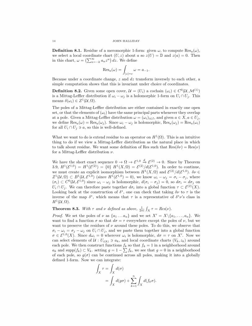
Definition 8.1. Residue of a meromorphic 1-form: given ω, to compute Resa(ω),we select a local coordinate chart (U, z) about a so z(U) = D and z(a) = 0. Thenin this chart, ω =
(∑∞n=−k anz
n)dz. We define
Resa(ω) =
∫|z|=ε
ω = a−1.
Because under a coordinate change, z and dz transform inversely to each other, asimple computation shows that this is invariant under choice of coordinates.
Definition 8.2. Given some open cover, U = (Ui) a cochain (ωi) ∈ C0(U ,M(1))is a Mittag-Leffler distribution if ωi − ωj is a holomorphic 1-form on Ui ∩Uj . Thismeans δ(ωi) ∈ Z1(U ,Ω).
The poles of a Mittag-Leffler distribution are either contained in exactly one openset, or that the elements of (ωi) have the same principal parts whenever they overlapat a pole. Given a Mittag-Leffler distribution ω = (ωi)i∈I , and given a ∈ X, a ∈ Uj ,we define Resa(ω) = Resa(ωj). Since ωi − ωj is holomorphic, Resa(ωj) = Resa(ωi)for all Ui ∩ Uj 3 a, so this is well-defined.
What we want to do is extend residue to an operator on H1(Ω). This is an intuitivething to do if we view a Mittag-Leffler distribution as the natural place in whichto talk about residue. We want some definition of Res such that Res(δν) = Res(ν)for a Mittag-Leffler distribution ν.
We have the short exact sequence 0 → Ω → E1,0 d−→ E(2) → 0. Since by Theorem3.9, H1(E1,0) = H1(E(2)) = 0 H1(X,Ω) = E(2)/d(E1,0). In order to continue,we must create an explicit isomorphism between H1(X,Ω) and E(2)/d(E1,0). δν ∈Z1(U ,Ω) ⊂ B1(U , E1,0) (since H1(E1,0) = 0), we know ωi − ωj = σi − σj , where(σi) ⊂ C0(U , E1,0) since ωi − ωj is holomorphic, d(σi − σj) = 0, so dσi = dσj on
Ui ∩ Uj . We can therefore paste together dσi into a global function τ ⊂ E(2)(X).Looking back at the construction of δ∗, one can check that taking δν to τ is theinverse of the map δ∗, which means that τ is a representative of δ∗ν’s class inH1(U ,Ω).
Theorem 8.3. With τ and ν defined as above, 12πi
∫Xτ = Res(ν).
Proof. We set the poles of ν as a1 . . . an and we set X ′ = X\a1, . . . , an. Wewant to find a function σ so that dσ = τ everywhere except the poles of ν, but wewant to preserve the residues of ν around these poles. To do this, we observe thatσi − ωi = σj − ωj on Ui ∩ Uj , and we paste them together into a global functionσ ∈ E1,0(X). Since dωi = 0 wherever ωi is holomorphic, dσ = τ on X ′. Now wecan select elements of U : Ui(k) 3 ak, and local coordinate charts (Vk, zk) aroundeach pole. We then construct functions fk so that fk = 1 in a neighborhood aroundak and supp(fk) ⊂ Vk. setting g = 1−
∑fk, we see that g = 0 in a neighborhood
of each pole, so g(σ) can be continued across all poles, making it into a globallydefined 1-form. Now we can integrate:∫
X
τ =
∫X
d(σ)
=
∫X
d(gσ) +
n∑k=1
∫X
d(fkσ).
THE RIEMANN-ROCH THEOREM AND SERRE DUALITY 15
By Stokes’ theorem,∫Xd(gσ) = 0. Since d(fkσ) = 0 wherever fk is constant, it is
zero in some ε neighborhood Nk of ak on which fk = 1 and some larger neighorhoodMk on which fk = 0. So, we have
n∑k=1
∫X
d(fkσ) =∑∫
Mk\Nk
d(fkσ)
=∑∫
∂Mk
fkσ −∫∂Nk
fkσ
= −∑∫
∂Nk(σi(k) − ωi(k)
)=∑
2πiResakωi(k)
= 2πiRes(ν).
Now we can define Res([δν]) = Res(ν), and we have successfully extended Res to alinear functional on H1(O).
8.2. The Proof of Serre Duality. Given a divisor D and an open U ⊂ X, ifξ ∈ Ω−D(X), η ∈ OD(U), ξ|Uη ∈ O(U). Thus, There is a map induced by ξ oncochains, and since this map takes coboundaries to coboundaries it induces a mapH0(ΩD) × H1(O−D) → H1(O). composing this with Res gets us a bilinear map〈 , 〉 : 〈η, ξ〉 = Res(ηξ). This induces a map iD : H0(ΩD) → H1(O−D)∗. We wantto show that this map is an isomorphism. Doing this in full is a long and technicalproof. We follow the proof in Chapter 17 of [3], and any details we leave out canbe found there.
Theorem 8.4. The map iD is injective.
Proof. We pick ω ∈ H0(ΩD), and consider any point p /∈ D∪(ω). We want to showthat ω is nonzero as an element of H1(O−D)∗, so we find some open cover and acochain ξ in that cover such that Res(ωξ) 6= 0. Since D∪ (ω) is an isolated, set, wecan pick an open set and coordinate (U0, z), such that U0 doesn’t intersect D∪ (ω)at all. So, locally ω = f(z)dz, where f ∈ O∗(U0), a holomorphic function whichis never zero in U0. Now we set U1 = X ∩ p, and U = U0, U1. Then we define(fi) ∈ C0(U ,M), where f0 = 1/(zf) and f1 = 0. Then δ(fi) ⊂ Z1(U ,O−D). Butωδ(fi) = dz/z on U0 ∩ U1, so Res(ωδ(fi)) = 1.
We know from the long exact sequence of cohomology groups that if we have aninclusion 0→ OD → OD′ then we have a surjection H1(OD′)→ H1(OD).10 Takingthe dual, we have a monomorphism of the dual groups
0→ H1(OD)∗iDD′−−→ H1(OD′)∗.
We assert the following detail-checking lemmas without proof:
10This is the inverse of the monomorphism induced by the long exact sequence.
16 JOHN HALLIDAY
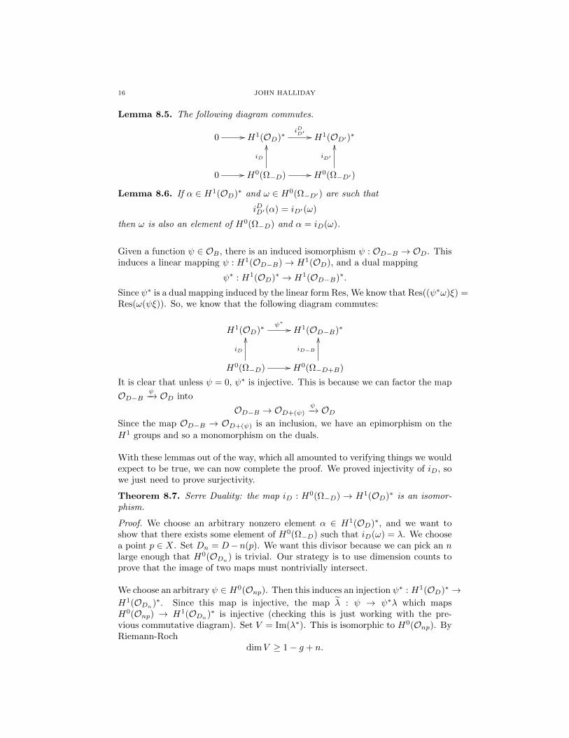
Lemma 8.5. The following diagram commutes.
0 // H1(OD)∗iDD′ // H1(OD′)∗
0 // H0(Ω−D) //
iD
OO
H0(Ω−D′)
iD′
OO
Lemma 8.6. If α ∈ H1(OD)∗ and ω ∈ H0(Ω−D′) are such that
iDD′(α) = iD′(ω)
then ω is also an element of H0(Ω−D) and α = iD(ω).
Given a function ψ ∈ OB , there is an induced isomorphism ψ : OD−B → OD. Thisinduces a linear mapping ψ : H1(OD−B)→ H1(OD), and a dual mapping
ψ∗ : H1(OD)∗ → H1(OD−B)∗.
Since ψ∗ is a dual mapping induced by the linear form Res, We know that Res((ψ∗ω)ξ) =Res(ω(ψξ)). So, we know that the following diagram commutes:
H1(OD)∗ψ∗ // H1(OD−B)∗
H0(Ω−D) //
iD
OO
H0(Ω−D+B)
iD−B
OO
It is clear that unless ψ = 0, ψ∗ is injective. This is because we can factor the map
OD−Bψ−→ OD into
OD−B → OD+(ψ)ψ−→ OD
Since the map OD−B → OD+(ψ) is an inclusion, we have an epimorphism on the
H1 groups and so a monomorphism on the duals.
With these lemmas out of the way, which all amounted to verifying things we wouldexpect to be true, we can now complete the proof. We proved injectivity of iD, sowe just need to prove surjectivity.
Theorem 8.7. Serre Duality: the map iD : H0(Ω−D) → H1(OD)∗ is an isomor-phism.
Proof. We choose an arbitrary nonzero element α ∈ H1(OD)∗, and we want toshow that there exists some element of H0(Ω−D) such that iD(ω) = λ. We choosea point p ∈ X. Set Dn = D−n(p). We want this divisor because we can pick an nlarge enough that H0(ODn
) is trivial. Our strategy is to use dimension counts toprove that the image of two maps must nontrivially intersect.
We choose an arbitrary ψ ∈ H0(Onp). Then this induces an injection ψ∗ : H1(OD)∗ →H1(ODn
)∗. Since this map is injective, the map λ : ψ → ψ∗λ which mapsH0(Onp) → H1(ODn)∗ is injective (checking this is just working with the pre-vious commutative diagram). Set V = Im(λ∗). This is isomorphic to H0(Onp). ByRiemann-Roch
dimV ≥ 1− g + n.
THE RIEMANN-ROCH THEOREM AND SERRE DUALITY 17
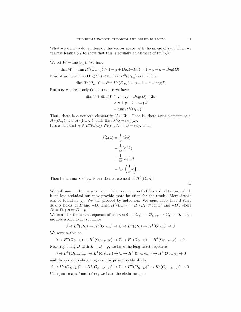
What we want to do is intersect this vector space with the image of iDn. Then we
can use lemma 8.7 to show that this is actually an element of Im(iD).
We set W = Im(iDn). We have
dimW = dimH0(Ω−Dn) ≥ 1− g + Deg(−Dn) = 1− g + n−Deg(D).
Now, if we have n so Deg(Dn) < 0, then H0(ODn) is trivial, so
dimH1(ODn)∗ = dimH1(ODn) = g − 1 + n− degD
But now we are nearly done, because we have
dimV + dimW ≥ 2− 2g −Deg(D) + 2n
> n+ g − 1− degD
= dimH1(ODn)∗
Thus, there is a nonzero element in V ∩ W . That is, there exist elements ψ ∈H0(Onp), ω ∈ H0(Ω−Dn), such that λ∗ψ = iDn(ω).It is a fact that 1
ψ ∈ H0(O(ψ)) We set D′ = D − (ψ). Then
iDD′(λ) =1
ψ(λψ)
=1
ψ(ψ∗λ)
=1
ψiDn
(ω)
= iD′
(1
ψω
).
Then by lemma 8.7, 1ψω is our desired element of H0(Ω−D).
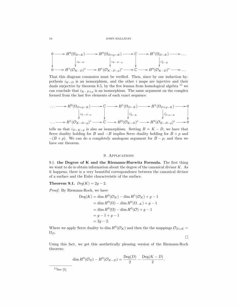
We will now outline a very beautiful alternate proof of Serre duality, one whichis no less technical but may provide more intuition for the result. More detailscan be found in [2]. We will proceed by induction. We must show that if Serreduality holds for D and −D. Then H0(Ω−D′) = H1(OD′)∗ for D′ and −D′, whereD′ = D + p or D − p.We consider the exact sequence of sheaves 0 → OD → OD+p → Cp → 0. Thisinduces a long exact sequence
That this diagram commutes must be verified. Then, since by our induction hy-pothesis iK−D is an isomorphism, and the other i maps are injective and theirduals surjective by theorem 8.5, by the five lemma from homological algebra 11 wecan conclude that iK−D+p is an isomorphism. The same argument on the complexformed from the last five elements of each exact sequence
tells us that iD−K−p is also an isomorphism. Setting B = K − D, we have thatSerre duality holding for B and −B implies Serre duality holding for B + p and−(B + p). We can do a completely analogous argument for B − p, and then wehave our theorem.
9. Applications
9.1. the Degree of K and the Riemann-Hurwitz Formula. The first thingwe want to do is obtain information about the degree of the canonical divisor K. Asit happens, there is a very beautiful correspondence between the canonical divisorof a surface and the Euler characteristic of the surface.
Theorem 9.1. Deg(K) = 2g − 2.
Proof. By Riemann-Roch, we have
Deg(K) = dimH0(OK)− dimH1(OK) + g − 1
= dimH0(Ω)− dimH0(Ω−K) + g − 1
= dimH0(Ω)− dimH0(O) + g − 1
= g − 1 + g − 1
= 2g − 2.
Where we apply Serre duality to dimH0(OK) and then the the mappings OD+K =ΩD.
Using this fact, we get this aesthetically pleasing version of the Riemann-Rochtheorem:
dimH0(OD)−H0(OK−D) =Deg(D)
2− Deg(K −D)
2.
11See [5].
THE RIEMANN-ROCH THEOREM AND SERRE DUALITY 19
The degree of K is extremely important. In fact, if we had chosen to prove it ina manner not requiring Serre duality, could immediately derive a weak version ofSerre duality from it. We do not get an explicit isomorphism, but we can provethat the groups in question have the same dimension. We only require theorem 8.5:that iD is injective.
Theorem 9.2. Weak version of Serre duality: dimH0(ΩD) = dimH1(O−D).
Proof. Since iD is injective, we have dimH0(ΩD) ≤ dimH1(O−D), so dimH0(OD+K) ≤dimH1(O−D). By Riemann-Roch, we know that
But since by above both dimH0(OD+K) − dimH1(O−D) and dimH0(O−D) −dimH1(OD+K) must be nonpositive, they both must be zero, so we get dimH0(OD+K)−dimH1(O−D) = 0 as desired.
We can use this degree to investigate the degree and branching of a function be-tween any two Riemann surfaces. We define the valency v(f, x) of f at a point xto be the multiplicity with which f takes the value f(x) at the point x. In otherwords, in local coordinates f looks like zk where k = v(f, x). We then defineB(f) =
∑x∈X v(f, x) − 1. at a typical point, there will be zero branching. If we
are on a compact Riemann surface, it is elementary Riemann surface theory thatthere can only be a finite number of branch points, and so B(f) is finite.
This next formula relates the genus two Riemann surfaces with the degree andbranching of a mapping between them.
Theorem 9.3. The Riemann-Hurwitz Formula: If f : X → Y is a analytic mapbetween Riemann surfaces, then gX − 1 = deg(f)(gY − 1) + 1
2B(f).
Proof. We can pull back a differential form ω from Y to X. from above, we knowDeg((ω)) = 2gY − 2 and Deg((f∗ω)) = 2gX − 2.
We select x ∈ X, designate f(x) = y and pick a coordinate chart (U, z) around xand (V,w) around y around which f = w = zk where k = v(f, x). Then on V , weset ω = φ(w)dw. f∗ω = φ(zk)kzk−1dz. Transforming w to zk multiplies the orderof ω by k and the zk−1 term adds k − 1 = b(f, x), so we get
ordx(f∗ω) = b(f, x) + v(f, x)ordy(ω).
v(f, x), when taken over all x = f−1(y), must total to the degree of f , so we get∑x=f−1(y)
ordx(f∗ω) =∑
x=f−1(y)
b(f, x) + deg fordy(ω).
Summing this over all y ∈ Y , we get∑x∈X
ordx(f∗ω) =∑x∈X
b(f, x) + n∑y∈Y
ordy(ω),
20 JOHN HALLIDAY
which simplifies to 2gX − 2 = deg f(2gY − 2) +B(f, x), or
gX − 1 = deg(f)(gY − 1) +1
2B(f).
Example 9.4. Let’s look at the Riemann surface generated by the equation n√
(1− zn),where z : P1 → P1 is the identity on the Riemann sphere. We want to determinethe genus of this surface. Rewriting the equation as
∏ni=1(z = ζi)
1/n, it is clearthere are n branch points, one at each of the nth roots of unity, and each one hasvalency n, and so branching number n− 1. since deg(f) = n, we get
gX − 1 = −n+n(n− 1)
2
gX = −(n− 1) +n(n− 1)
2
=(n− 2)(n− 1)
2.
This result is a special case of the degree-genus formula.
9.2. Applications to Riemann Surfaces. Serre duality and Riemann-Roch arebeautiful results in and of themselves, but where they really shine is their usefulnessin computations. We give a few examples.
Theorem 9.5. Any Riemann surface X of genus g is at most a g + 1-branchedcover of the Riemann-sphere.
Proof. This statement is equivalent to there being a non-constant f of degree atmost g + 1 on X (remember that a meromorphic function is just an analytic mapto the Riemann sphere.) If we consider the divisor D = (g + 1)p for some p ∈ X,we have
dimH0(OD) ≥ 1− g + Deg(D) = 2.
So there must be a non-constant element f which is a meromorphic function withonly one pole of degree at most g + 1.
In particular, since a degree one covering map is an isomorphism, we have proventhat every genus zero algebraic curve is isomorphic to the Riemann sphere.
Theorem 9.6. Every genus one Riemann surface is isomorphic to a complex torus.
Proof. Call our surface X. A complex torus is a quotient C by the group actions〈z → z+ω1〉, 〈z → z+ω2〉 where ω1ω2 are R-linear independent. Since our surfacewhen seen as a real 2-manifold has genus one and is therefore topologically a torus,we know it has a universal cover X = R2, with π : X → X the covering map. Allwe have to show is that X = C as a Riemann surface and we have our proof, sincethe Deck transformations must take the form of the group actions above.
We consider a meromorphic 1-form ω on X. since Deg((ω)) = 0 since it is acanonical divisor, we have by Riemann-Roch
dimH0(O(ω))− dimH0(O) = 1− g + degD dimH0(O(ω)) = 1.
If we select f ∈ H0(O(ω)) we know (f) ≥ −(ω), so (fω) ≥ 0, which means fωis a holomorphic 1-form. since Deg(fω) = 0 since it is a meromorphic function
THE RIEMANN-ROCH THEOREM AND SERRE DUALITY 21
multiplied by a meromorphic 1-form, we know that (fω) = 0, so it is a 1-form with
no zeroes or poles. Now, consider the pullback π∗(fω). fix a point p0 ∈ X and defineφ(p) =
∫ pp0π∗(fω). Since π∗(fω) is still a holomorphic 1-form, the given integral
only depends on its endpoints, so is well-defined. The integral of a holomorphic1-form is holomorphic, so φ is an isomorphism between X and C as desired.
A curve is called hyperelliptic if it can be seen as a double-cover of the Riemannsphere.
Theorem 9.7. Any genus two Riemann surface is hyperellipic.
Proof. Clearly a curve is hyperelliptic if it admits a degree two meromorphic func-tion. For a genus two curve, we have
dimH0(Ω) = dimH0(OK)
= 1− g + Deg(K) + dimH0(O))
= 1− 2 + 2 + 1 = 2
so there is a non-constant holomorphic 1-form ω. Now say K = ω. This meansK ≥ 0, and since as above we know dimH0(OK) = 2, there is a nonconstantmeromorphic function f ∈ H0(OK). f can have a pole of order at most 2, andcannot have solely poles of degree 1 or it would be isomorphic to the Riemannsphere, so we have found our double-cover.
10. Conclusion
The Riemann-Roch theorem and Serre duality are very powerful tools in complexand algebraic geometry. Additional structures such as the Jacobi variety and thePicard group are natural things to investigate after learning this material, andprovide further geometric tools to work with. The theory of vector bundles is avery useful persepctive that we regrettably could not discuss in this paper. Learningthe vector bundle perspective on this material lets one view any of the sheaveOD as the sheaf of sections of some vector bundle. The theory of sheaves andsheaf cohomology is very important in algebraic geometry, but its most generalform is more complicated than the version we have presented here. For more onthis, see [4]. The Riemann-Roch theorem and Serre duality also have powerfulgeneralizations. For higher dimensional complex manifolds, the Riemann-Rochtheorem still appears as a statement about the Euler characteristic of a sheaf,but more powerful machinery than we develop here is required to state any of itsgeneralizations. We see the true ”duality” provided by Serre duality when viewingits statement on a complex manifold of dimension n: Hi(OD) ∼= Hn−i(OK−D).Studying this material from either a complex geometric or algebraic perspectivereveals powerful generalizations of all of the material we have discussed, but theextremely well-behaved theory of Riemann surfaces is an excellent place to first seethese ideas in their more elementary form.
11. Acknowledgments
It is a pleasure to thank my mentor, Sergei Sagatov for his excellent guidanceand assistance over the summer. I would like to thank Peter May for hosting theREU and making this paper possible.
22 JOHN HALLIDAY
References
[1] Raoul Bott and Loring W. Tu. Differential Forms in Algebraic Topology. Springer, 1982.[2] Simon Donaldson. Riemann Surfaces. Oxford University Press. 2011
[3] Otto Forster. Lectures in Riemann Surfaces Springer, 1981.
[4] Robin Hartshorne. Algebraic Geometry. Springer 1977[5] Williams S. Massey.f A Basic Course in Algebraic Topology. Springer, 1991.
[6] Rick Miranda. Algebraic Curves and Riemann Surfaces American Mathematical Society, 1995.
[7] Wilhelm Schlag. A Course in Complex Analysis and Riemann Surfaces. American Mathemat-ical Society, 2014.