The Risk-Adjusted Cost of Financial Distress

Heitor Almeida and Thomas Philippon∗

Abstract

Financial distress is more likely to happen in bad times. The present value of distress costs thereforedepends on risk premia. We estimate this value using risk-adjusted default probabilities derivedfrom corporate bond spreads. For a BBB-rated firm, our benchmark calculations show that therisk-adjusted NPV of distress is 4.5% of pre-distress firm value. In contrast, a valuation that ignoresrisk premia produces an NPV of 1.4%. We show that risk-adjusted, marginal distress costs can beas large as the marginal tax benefits of debt derived by Graham (2000). Thus, distress risk premiacan help explain why firms appear to use debt conservatively.

∗ Heitor Almeida and Thomas Philippon are at the Stern School of Business, New York University and theNational Bureau of Economic Research. We wish to thank an anonymous referee for insightful comments andsuggestions. We also thank Viral Acharya, Ed Altman, Yakov Amihud, Long Chen, Pierre Collin-Dufresne,Joost Driessen, Espen Eckbo, Marty Gruber, Jing-Zhi Huang, Tim Johnson, Augustin Landier, FrancisLongstaff, Lasse Pedersen, Matt Richardson, Pascal Maenhout, Chip Ryan, Tony Saunders, Ken Singleton,Rob Stambaugh, Jos Van Bommel, Ivo Welch, and seminar participants at the University of Chicago, MIT,Wharton, Ohio State University, London Business School, Oxford Said Business School, USC, New YorkUniversity, the University of Illinois, HEC-Paris, HEC-Lausanne, Rutgers University, PUC-Rio, the 2006WFA meetings, and the 2006 Texas Finance Festival for valuable comments and suggestions. We also thankEd Altman and Joost Driessen for providing data. All remaining errors are our own.

Financial distress has both direct and indirect costs (Warner, 1977, Altman, 1984, Franks and

Touros, 1989, Weiss, 1990, Asquith, Gertner and Scharfstein, 1994, Opler and Titman, 1994,

Sharpe, 1994, Denis and Denis, 1995, Gilson, 1997, Andrade and Kaplan, 1998, Maksimovic and

Phillips, 1998). However, whether such costs are high enough to matter for corporate valuation

practices and capital structure decisions is hotly debated. Direct costs of distress, such as litigation

fees, are relatively small.1 Indirect costs, such as loss of market share (Opler and Titman, 1994) and

inefficient asset sales (Shleifer and Vishny, 1992), are believed to be more important, but they are

also much harder to quantify. In a sample of highly leveraged firms, Andrade and Kaplan (1998)

estimate losses in value given distress on the order of 10% to 23% of pre-distress firm value.2

Irrespective of their exact magnitudes, ex-post losses due to distress must be capitalized to

assess their importance for ex-ante capital structure decisions. The existing literature argues that

even if ex-post losses amount to 10% to 20% of firm value, ex-ante distress costs are modest because

the probability of financial distress is very small for most public firms (Andrade and Kaplan, 1998,

Graham, 2000). In this paper, we propose a new way of calculating the NPV of financial distress

costs. Our results show that the existing literature has substantially underestimated the magnitude

of ex-ante distress costs.

A standard method of calculating ex-ante distress costs is to multiply Andrade and Kaplan’s

(1998) estimates of ex-post costs by historical probabilities of default (Graham, 2000, Molina,

2005), but this calculation ignores capitalization and discounting. Other researchers have assumed

risk neutrality and have discounted the product of historical probabilities and losses in value given

default by a risk-free rate (e.g., Altman (1984)).3 This calculation, however, ignores the fact that

distress is more likely to occur in bad times.4 Thus, risk-averse investors should care more about

financial distress than is suggested by risk-free valuations. Our goal in this paper is to quantify the

impact of distress risk premia on the NPV of distress costs.

Our approach is based on the following insight: to the extent that financial distress costs occur

in states of nature in which bonds default, one can use corporate bond prices to estimate the distress

risk adjustment. The asset pricing literature has provided substantial evidence for a systematic

component in corporate default risk. It is well known that the spread between corporate and

government bonds is too high to be explained only by expected default and that it reflects in part a

large risk premium (Elton, Gruber, Agrawal and Mann, 2001, Huang and Huang, 2003, Longstaff,

1

Mittal, and Neis, 2005, Driessen, 2005, Chen, Collin-Dufresne, and Goldstein, 2005, Cremers,

Driessen, Maenhout and Weinbaum 2005, Berndt, Douglas, Duffie, Ferguson, and Schranz, 2005).5

As in standard calculations, our new methodology assumes the estimates of ex-post distress

costs provided by Andrade and Kaplan (1998) and Altman (1984). Unlike those calculations,

however, this method uses observed credit spreads to back out the market-implied, risk-adjusted

(or risk-neutral) probabilities of default. Such an approach is common in the credit risk literature

(i.e., Duffie and Singleton, 1999, and Lando, 2004). Our calculations also consider tax and liquidity

effects (Elton et al., 2001, Chen, Lesmond, and Wei, 2004) and use only the fraction of the spread

that is likely to be due to default risk.

Our estimates suggest that risk-adjusted probabilities of default and, consequently, the risk-

adjusted NPV of distress costs, are considerably larger than historical default probabilities and

the non risk-adjusted NPV of distress, respectively. Consider for instance a firm whose bonds are

rated BBB. In our data, the historical 10-year cumulative probability of default for BBB bonds

is 5.22%. However, in our benchmark calculations the 10-year cumulative risk-adjusted default

probability implied by BBB spreads is 20.88%. This large difference between historical and risk-

adjusted probabilities translates into a substantial difference in NPVs of distress costs. Using the

average loss in value given distress from Andrade and Kaplan (1998), our NPV formula implies a

risk-adjusted distress cost of 4.5%. For the same ex-post loss, the non risk-adjusted NPV of distress

is only 1.4% for BBB bonds.

Our results have implications for capital structure. In particular, they suggest that the marginal,

risk-adjusted distress costs can be of the same magnitude as the marginal tax benefits of debt

computed by Graham (2000). For example, using our benchmark assumptions the increase in risk-

adjusted distress costs associated with a change in ratings from AA to BBB is 2.7% of pre-distress

firm value.6 To compare this number with marginal tax benefits of debt, we derive the marginal

tax benefit of leverage that is implicit in Graham’s (2000) calculations and use the relationship

between leverage ratios and bond ratings recently estimated by Molina (2005). The implied gain

in tax benefits as the firm moves from an AA to a BBB rating is 2.67% of firm value. Thus, it

is not clear that the firm gains much by increasing leverage from AA to BBB levels.7 These large

estimated distress costs may help explain why many US firms appear to be conservative in their

use of debt, as suggested by Graham (2000).

2

This paper proceeds as follows. We first present a simple example of how our valuation approach

works. The general methodology is presented in Section II, followed by our empirical estimates of

the NPV of distress costs in Section III, and various robustness checks in Section IV. Section V

discusses the capital structure implications of our results, and we summarize our findings in Section

VI.

I. Using Credit Spreads to Value Distress Costs: A SimpleExample

In this section, we explain our procedure with a simple example. The purpose of the example

is both to illustrate the intuition behind our general procedure (Section II) and to provide simple

back-of-the-envelope formulas that can be used to value financial distress costs. The formulas are

easy to implement and provide a reasonable approximation of the more precise formulas derived

later. We start with a one-period example and then present an infinite horizon example.

A. One-period Example

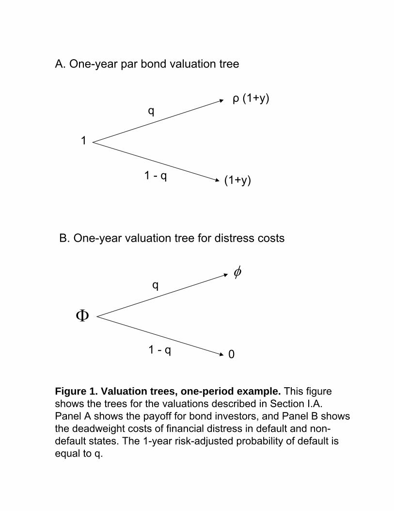
Suppose that we want to value distress costs for a firm that has issued an annual-coupon bond

maturing in exactly one year. The bond’s yield is equal to y, and the bond is priced at par. The

bond’s recovery rate, which is known with certainty today, is equal to ρ. Thus, if the bond defaults,

creditors recover ρ(1 + y). The bond’s valuation tree is depicted in Figure 1. The value of the

bond equals the present value of expected future cash flows, adjusted for systematic default risk. If

we let q be the risk-adjusted (or risk-neutral), one-year probability of default, we can express the

bond’s value as:

1 =(1− q)(1 + y) + qρ(1 + y)

1 + rF, (1)

where rF is the one-year risk-free rate.

[Insert Figure 1 here]

In the valuation formula (1), the probability q incorporates the default risk premium that is

implicit in the yield spread y − rF . If investors were risk neutral, or if there was no systematic

3

default risk, q would be equal to the expected probability of default which we denote by If default

risk is priced, then the implied q is higher than Equation (1) can be solved for q:

q =y − rF

(1 + y)(1− ρ). (2)

The basic idea in this paper is that we can use the risk-neutral probability of default, q, to

perform a risk-adjusted valuation of financial distress costs. Consider again Figure 1, which also

depicts the valuation tree for distress costs. Let the loss in value given default be equal to φ and

the present value of distress costs be equal to Φ. For simplicity, suppose that φ is known with

certainty today. If we assume that financial distress can only happen at the end of one year, but

never again in future years, then we can express the present value of financial distress costs as:

Φ =qφ+ (1− q)01 + rF

. (3)

Formula (3) is similar to that used by Graham (2000) and Molina (2005) to value distress costs. The

key difference is that while Graham (2000) and Molina (2005) used historical default probabilities,

equation (3) uses a risk-adjusted probability of financial distress that is calculated from yield spreads

and recovery rates using equation (2).

B. Infinite Horizon Example

To provide a more precise estimate of the present value of financial distress costs, we must

recognize that if financial distress does not occur at the end of the first year, it can still happen in

future years. If we assume that the marginal risk-adjusted default probability q and the risk-free

rate rF do not change after year one,8 then the valuation tree becomes a sequence of one-year

trees that are identical to that depicted in Figure 1. This implies that if financial distress does

not happen in year one (an event that happens with probability 1− q) the present value of future

distress costs at the end of year one is again equal to Φ. Replacing 0 with Φ in the valuation

equation (3) and solving for Φ, we obtain:

Φ =q

q + rFφ. (4)

Equation (4) provides a better approximation of the present value of financial distress costs than

does equation (3). Notice also that for a given q (that is, irrespective of the risk adjustment),

equation (3) substantially underestimates the present value of distress costs.

4

The assumptions that q and rF do not vary with the time horizon are counterfactual. The

general procedure that we describe later allows for a term structure of q and rF . For the purpose of

illustration, however, suppose that q and rF are indeed constant. In the appendix, we spell out the

conditions under which equation (2) can be used to obtain the (constant) risk-adjusted probability

of default q.

To illustrate the impact of the risk adjustment, take the example of BBB-rated bonds. In our

data, the historical average 10-year spread on those bonds is approximately 1.9%, and the historical

average recovery rate is equal to 0.41.9 As we discuss in the next section, the credit risk literature

suggests that this spread cannot be attributed entirely to default losses because it is also affected

by tax and liquidity considerations. Essentially, our benchmark calculations remove 0.51% from

this raw spread.10 The difference (1.39%) is what is usually called the default component of yield

spreads. Using this default component, a recovery of 0.41, and a long-term interest rate of 6.7%

(the average 10-year treasury rate in our data), equation (2) gives an estimate for q equal to 2.2%.

Using historical data to estimate the marginal default probability yields much lower values. For

example, the average marginal default probability over time horizons from 1 to 10 years for bonds of

an initial BBB rating is equal to 0.53% (Moody’s, 2002). The large difference between risk-neutral

and historical probabilities suggests the existence of a substantial default risk premium.

As discussed in the introduction, the literature has estimated ex-post losses in value given

default (the term φ) of 10% to 23% of pre-distress firm value. If we use, for example, the midpoint

between these estimates (φ = 16.5%), the NPV of distress for the BBB rating goes from 1.2%

(using historical probabilities) to 4.1% (using risk-adjusted probabilities). Clearly, incorporating

the risk adjustment makes a large difference to the valuation of financial distress costs. We now

turn to the more general model to see if this conclusion is robust.

II. General Valuation Formula

Figure 2 illustrates the timing of the general model that we use to value financial distress costs.

Our goal is to calculate Φ0, the NPV of distress costs at an initial date (date 0). In Figure 2, φ0,t

is the deadweight loss that the firm incurs if distress happens at time t, where t = 1, 2....

[Insert Figure 2 here]

5

In all of our analysis, we assume that distress states and default states are the same. Thus, our

calculations apply to the distress costs that are incurred upon or after default. This assumption

is consistent with the results in Andrade and Kaplan (1998), who report that 26 out of the 31

distressed firms in their sample either default or restructure their debt in the year that the authors

classify as the onset of financial distress. Nonetheless, we acknowledge that our approach might not

capture some of the indirect costs of distress that are incurred before default (i.e., Titman (1984)).

To be consistent with Andrade and Kaplan (1998), who measure the value lost at the onset of

distress, we define φ0,t as the expectation at time 0 of the capitalized distress costs that occur after

default at time t. After default, the firm might reorganize or it might be liquidated. If the firm

does not default at time t, it moves to period t+ 1, and so on.

We let q0,t be the risk-adjusted, marginal probability of distress (default) in year t, conditional

on no default until year t− 1, and evaluated as of date 0. In contrast with Section I, we now allow

q0,t to vary with the time horizon. We also define (1−Q0,t) =Qts=1(1− q0,s) as the risk-adjusted

probability of surviving beyond year t, evaluated as of date 0. Conversely, Q0,t is the cumulative

risk-adjusted probability of default before or during year t. The probability that default occurs

exactly at year t is thus equal to (1 − Q0,t−1)q0,t. Throughout the paper, we will maintain the

following assumption:

assumption 1: The deadweight loss φ0,t in case of default is constant, φ0,t = φ.

In particular, this assumption implies that there is no systematic risk associated with φ. As-

sumption 1 could lead us to underestimate the distress risk adjustment if the deadweight losses

conditional on distress are higher in bad times, as suggested by Shleifer and Vishny (1992). How-

ever, it is also possible that deadweight losses are higher in good times because financial distress

might cause the firm to lose profitable growth options (Myers, 1977).

Under assumption 1, we can write the NPV of financial distress as:

Φ0 = φXt≥1

B0,t(1−Q0,t−1)q0,t , (5)

where B0,t is the price at time zero of a riskless zero-coupon bond paying one dollar at date t.

Equation (5) gives the ex-ante value of financial distress as a function of the term structure of

distress probabilities and risk-free rates. In Section III.D, we estimate the average value of Φ0

6

using the historical average term structures of B0,t and Q0,t, and in Section IV.F we discuss the

impact of time variation in the price of credit risk.

A. From Credit Spreads to Probabilities of Distress

As in Section I, we use observed corporate bond yields to estimate the risk-adjusted default

probabilities used in equation (5). Specifically, suppose that we observe at date 0 an entire term

structure of yields for the firm whose distress costs we want to value; that is, we know the sequence©yt0ªt=1,2...

, where yt0 is the date-0 yield on a corporate bond of maturity t. In addition, suppose

we know the coupons©ctªt=1,2...

associated with each bond maturity.11 For now, we assume that

the entire spread between yt0 and the reference risk-free rate is due to default losses and relegate

the discussion of tax and liquidity effects to Section III. By the definition of the yield, the date-0

value of the bond of maturity t, V t0 , is

V t0 =ct

(1 + yt0)+

ct

(1 + yt0)2+ ...+

1 + ct

(1 + yt0)t. (6)

A.1. Bond Recovery

We let ρtτ be the dollar amount recovered by creditors if default occurs at date τ ≤ t for a bond

of maturity t. As discussed by Duffie and Singleton (1999), to obtain risk-neutral probabilities from

the term structure of bond yields, we need to make specific assumptions about bond recoveries.

Our benchmark valuation uses the following assumption, which was originally employed by Jarrow

and Turnbull (1995):

assumption 2: Constant recovery of treasury (RT). In case of default, the creditors recover ρtτ =

ρP tτ , where Ptτ is the price at date τ of a risk-free bond with the same maturity and coupons as the

defaulted bond and ρ is a constant.

The idea behind assumption 2 is that default does not change the timing of the promised

cash flows. When default occurs, the risky bond is effectively replaced by a risk-free bond whose

cash flows are a fraction ρ of the cash flows promised initially. In Section IV.B, we discuss other

assumptions commonly used in the credit risk literature and we show that our results are robust.

The assumption that ρ is constant is similar to our previous assumption that φ is constant. However,

there is some evidence in the literature that recovery rates tend to be lower in bad times (Altman et

7

al., 2003, Allen and Saunders, 2004, Acharya et al., 2005). We verify in Section IV.A the robustness

of our results to the introduction of recovery risk.

A.2. Risk-Neutral Probabilities

Our next task is to derive the term structure of risk-neutral probabilities from observed bond

prices. We do so recursively. Under assumption 2, the price V 10 of a one-year bond must satisfy

V 10 = [(1−Q0,1) +Q0,1ρ] (1 + c1)B0,1. (7)

This equation gives Q0,1 as a function of known quantities. Given {Q0,τ}τ=1..t, we show in the

appendix that the value of a bond with maturity t+ 1 is

V t+10 =tX

τ=1

[(1−Q0,τ ) +Q0,τρ]ct+1B0,τ + [(1−Q0,t+1) +Q0,t+1ρ]¡1 + ct+1

¢B0,t+1. (8)

This equation can be inverted to obtain Q0,t+1. Therefore, we can recursively derive the sequence

of risk-adjusted probabilities {Q0,t}t=1,2... from©V tªt=1,2...

,©ctªt=1,2...

, {B0,t}t=1,2..., and ρ. This

procedure allows us to generalize equation (2). The risk-adjusted probabilities can then be used to

value distress costs using equation (5).

III. Empirical Estimates

We begin by describing the data used in the implementation of equations (5) and (8).

A. Data on Yield Spreads, Recovery Rates, and Default Rates

We obtained data on corporate yield spreads over treasury bonds from Citigroup’s yield book,

which covers the period 1985-2004. These data are available for bonds rated A and BBB, separately

for maturities 1-3, 3-7, 7-10, and 10+ years. For bonds rated BB and below, these data are available

only as an average across all maturities. Because the yield book records AAA and AA as a single

category, we rely on Huang and Huang (2003) to obtain separate spreads for the AAA and AA

ratings. Table I in Huang and Huang reports average 4-year spreads for 1985-1995 from Duffee

(1998) and average 10-year spreads for the period 1973-1993 from the Lehman’s bond index. For

consistency, we calculate our own averages from the yield book over the period 1985-1995, but we

note that average spreads are similar over periods 1985-1995 and 1985-2004.12 For all ratings, we

8

linearly interpolate the spreads to estimate the maturities that are not available in the raw data.

We assume constant spreads across maturities for BB and B bonds. The spread data used in this

study are reported in Table I.

[Insert Table I here]

Our benchmark valuation is based on the average historical spreads in Table I. Thus, the

resulting NPVs of distress should be seen as unconditional estimates of ex-ante distress costs for

each bond rating. We discuss the implications of time variation in yield spreads in Section IV.F.

We also obtained data on average treasury yields and zero coupon yields on government bonds

of different maturities from FRED and from JP Morgan. Because high expected inflation in the

1980s had a large effect on government yields, we use a broad time period (1985-2004) to calculate

these yields.13 Treasury data are available for maturities 1, 2, 3, 5, 7, 10, and 20 years, and zero

yields are available for all maturities between 1 and 10 years. Again, we used a simple linear

interpolation for missing maturities between 1 and 10 years.

Finally, we obtained historical cumulative default probabilities from Moody’s (2002). These

data are available for 1-year to 17-year horizons for bonds of initial ratings ranging from AAA

to B and refer to averages over the period 1970-2001. These default data are similar to those

used by Huang and Huang (2003).14 While these data are not used directly for the risk-adjusted

valuations, they are useful for comparison purposes. Moody’s (2002) also contains a time series of

bond recovery rates for the period 1982-2001.15 In most of our calculations we assume a constant

recovery rate, which we set to its historical average of 0.413.

B. Default Component of Yield Spreads

There is an ongoing debate in the literature about the role of default risk in explaining yield

spreads such as those reported in Table I. Because treasuries are more liquid than corporate bonds,

part of the spread should reflect a liquidity premium (see Chen et al., 2004). Also, treasuries have a

tax-advantage over corporate bonds because they are not subject to state and local taxes (Elton et

al., 2001). These arguments suggest that we cannot attribute the entire spreads reported in Table

I to default risk.

9

Researchers have attempted to estimate the default component of corporate bond spreads using

a number of different strategies. Huang and Huang (2003) use a calibration approach and found

that the default component predicted by many structural models is relatively small.16 In contrast,

Longstaff et al. (2005) argue that credit default swap (CDS) premia are a good approximation of

the default components, and suggest that the default component of spreads is much larger than

that suggested by Huang and Huang. Chen et al. (2005) use structural credit risk models with a

counter-cyclical default boundary and show that such models can explain the entire spread between

BBB and AAA bonds when calibrated to match the equity risk premium. Cremers et al. (2005)

add jump risk to a structural credit risk model that is calibrated using option data and generate

credit spreads that are much closer to CDS premiums than those generated by the models in Huang

and Huang. We summarize these recent findings in Table II. With the exception of Huang and

Huang, the findings in these papers appear to be reasonably consistent with each other.

Unfortunately, these papers report default components only for a subset of ratings and maturities.17

Thus, to implement formulas (5) and (8), we must first estimate the default component across all

ratings and maturities. We now present two ways to do so.

B.1. Method 1: Using the 1-year AAA Spread

Following Chen et al. (2005), we assume that the component of the spread that is not given

by default can be inferred from the spreads between AAA bonds and treasuries. Chen et al. use a

4-year maturity in their calculations, but our data on historical default probabilities suggest that,

while there has never been any default for AAA bonds up to a 3-year horizon, there is already a

small probability of default at a 4-year horizon (0.04%). Thus, it seems appropriate to use a shorter

spread to adjust for taxes and liquidity.18 The 1-year spread in Table I is 0.51%, and we calculate

the default components for rating i and maturity t as

(Default component)ti = (spread)ti − 0.51%. (9)

Notice that formula (9) allows us to construct spread default components for all ratings and ma-

turities. Table II reports some of the fractions implied by this procedure for select maturities. By

construction, the 4-year BBB fraction is virtually identical to that estimated by Chen et al.. Most

of the other fractions are very close to those estimated by Longstaff et al. (2005) and Cremers et

10

al. (2005), suggesting that method 1 produces default components that closely approximate CDS

premia. The only real discrepancy is with respect to Huang and Huang (2003), who estimate lower

fractions for investment-grade bonds.

[Insert Table II here]

B.2. Method 2:Using Spreads Over Swaps

As discussed above, Longstaff et al. (2005) argue that CDS premia are a good approximation for

the default component of yield spreads. In addition, Blanco et al. (2005) show that the spread over

swaps tracks CDS premia very closely. These results suggest that one can use spreads over swaps to

estimate the default component. Unfortunately, data on swap rates start only in 2000. Therefore,

we cannot use Huang and Huang’s spread data (which refers to 1985-1995) and consequently can

only provide fraction estimates for A, BBB, BB, and B-rated bonds. Using swap data for 2000-2004,

we calculate the average default component for rating i and maturity t as

(Fraction due to default)ti =(spread)ti − (swapt − treasuryt)

(spread)ti. (10)

Table II shows that this alternative approach gives fractions due to default that are very close to

those obtained using the AAA spread of method 1.19 Given these results, it seems safe to choose

method 1 as our benchmark approach to calculate default components. An important advantage

of method 1 is that it allows us to present valuations for all bond ratings, from AAA to B.

C. Risk-Neutral Probabilities and Excess Returns

Starting from the spreads reported in Table I, we use equation (9) to estimate the default

components, and then we use the default components to derive a term structure of risk-adjusted

default probabilities. Each bond yield yt0 is computed as the sum of the default component and

the corresponding treasury rate. We must make an assumption about coupon rates in order to use

equation (6). Our baseline calculations assume that corporate bonds trade at par, so that ct = yt0

and V t0 = 1 for all t. We then use equation (8) to generate a sequence of cumulative probabilities

of default {Q0,t}t=1,2..10.

11

Table III reports the risk-adjusted cumulative default probabilities for select maturities. For

comparison purposes, we also report the historical cumulative probabilities of default from Moody’s

(2002). The risk-adjusted, market-implied probabilities are larger than the historical ones for all

ratings and maturities and are substantially so for investment-grade bonds. For instance, the 5-year

historical default probability of BBB bonds is 1.95%, while the risk-neutral one is 11.39%. The

ratio between risk-neutral and historical probabilities (averaged over maturities) ranges from 3.57

for AAA-rated bonds to 1.21 for B-rated bonds. These ratios indicate the presence of a large credit

risk premium. Interestingly, the ratios are highest for investment-grade bonds, especially for the

AA, A, and BBB ratings. Cremers et al. (2005) suggest one possible interpretation of this pattern:

if the default risk premium is associated with a jump risk premium, it is perhaps not surprising

that the risk premium is lower for bonds that are quite likely to default (i.e., BB and B ratings).

[Insert Table III here]

The evidence on holding period excess returns of corporate bonds is also consistent with the

existence of the risk premium that we emphasize. Keim and Stambaugh (1986), for example,

find that excess returns of BBB bonds over long term government bonds are on average 8 basis

points a month in the period of 1928-1978. This excess return is equivalent to approximately 1% a

year. Fama and French (1989, 1993) report similar summary statistics for average excess returns.20

These numbers are largely consistent with the risk-neutral and historical probabilities in Table III.

Consider for example the excess return on a zero-coupon security that promises one dollar in 5

years, and defaults like a BBB bond. The risk-adjusted and historical probabilities in Table III

imply an annual expected excess return of 1.24% for this security,21 which is close to the average

historical excess returns that the literature reports..

D. Valuation

We can now use the term structure of risk-neutral probabilities computed in Section III.C in

the valuation equation (5). Because we only have cumulative default probabilities up to year 10,

we compute a terminal value of financial distress costs at year 10 (details in the appendix). The

terminal value is computed by assuming constant marginal risk-adjusted default probabilities and

12

yearly risk-free rates after year 10. Thus, the formula is very similar to that derived in the infinite

horizon example of Section I. As in Section I, we use φ = 16.5% in our benchmark calculations.

Graham (2000) and Molina (2005) use numbers in this range to compare tax benefits of debt and

costs of financial distress.

[Insert Table IV here]

The second column of Table IV presents our estimates of the risk-adjusted cost of financial

distress for different bond ratings. For comparison, we report in the first column the same valuations

using the historical default rates.22 We find that risk is a first-order issue in the valuation of distress

costs, which confirms the results of Section I. For instance, distress costs for the BBB rating increase

from 1.40% to 4.53% once we adjust for risk. To provide some evidence on the marginal increase

in distress costs as the firm moves across ratings, we also report the difference in distress costs

between the BBB and the AA rating. An increase in leverage that moves a firm from AA to BBB

increases the cost of distress by 2.7%. In contrast, the increase is only 1.11% if we use historical

probabilities. Thus, risk adjustment also matters for marginal distress costs.

IV. Robustness Checks

The estimates in Table IV rely on a set of assumptions about bond recoveries, coupon rates, and

deadweight losses given distress. We now check how sensitive our results are to these assumptions.

A. Recovery Risk

Following assumption 2, the benchmark valuation in the second column of Table IV uses ρ =

0.413 in equation (8). The use of an average historical recovery is common in the credit risk

literature. Huang and Huang (2003), Chen et al. (2005), and Cremers et al. (2005), for example,

use average historical recoveries of 0.51 in their calibrations. However, there is some evidence in the

literature of a systematic component of recovery risk (Altman et al., 2003, and Allen and Saunders,

2004). As discussed by Berndt et al. (2005) and Pan and Singleton (2005), a standard way to

incorporate recovery risk into credit risk models is to use a constant risk-neutral (as opposed to

average historical) recovery rate. Berndt et al. (2005) use a risk-neutral recovery rate of 0.25, which

13

is the lowest cross-sectional sample mean of recovery reported by Altman et al (2003). According to

Pan and Singleton (2005), this is a common industry standard for the risk-neutral recovery rate.23

We note that the lower the recovery rate plugged into equation (8), the lower the implied risk-

neutral probabilities. Low recoveries increase a creditor’s loss given default, and thus for a given

spread the implied probability of default is higher (see, for example, equation 2). The third column

of Table IV reports the results of decreasing the recovery rate to 0.25 without changing the estimate

for φ. As expected, the risk-adjusted costs of financial distress decrease.24 For example, the point

estimate for the BBB rating goes from 4.53% to 3.70% if bond recovery goes from 0.41 to 0.25.

Nonetheless, the risk adjustment is still large, and assuming a lower recovery does not affect the

estimated marginal costs of distress much. For example, if bond recovery is 0.25, the increase in

distress costs for a firm moving from AA to BBB is 2.2%, which is only slightly lower than the

corresponding margin when recovery is 0.41 (2.7%). We conclude that our results are robust to the

introduction of recovery risk.

B. Recovery of Face Value

Equation 8 is derived under the assumption that recovery is a fraction of a similar risk-free bond

assumption 2, or RT assumption). Another commonly used assumption is that recovery is a fraction

of the face value of the bond, with zero recovery of coupons (assumption RFV). In the appendix,

we show how to derive the term structure of risk-neutral probabilities from the default component

of the spreads under assumption RFV. The fourth column of Table IV shows the valuation results

with this alternative assumption. The implied risk-neutral probabilities of default are lower, and

thus the valuation results are slightly lower than those obtained under RT. However, it is clear from

the fourth column that the two assumptions generate very similar costs of financial distress. The

AA minus BBB margin, for example, goes from 2.69% (under RT) to 2.47% (RFV). We conclude

that the valuation is robust to alternative recovery assumptions.

C. Coupon Rates

The risk-neutral probabilities in Table III are derived under the assumption that the bond

coupons are equal to the adjusted bond yields (the default component of the yield plus the corre-

sponding treasury rate). To show the robustness of our results, Table IV contains the valuations

14

assuming that coupons are equal to 0.5 times the adjusted yields (in the fifth column) or 1.5 times

the adjusted yields (in the sixth column). Risk-adjusted probabilities, and thus risk-adjusted dis-

tress costs, are higher with higher coupons. However, it is clear from Table IV that the results are

relatively robust to variations in coupon rates. The BBB minus AA margin, for example, goes from

2.64% (when coupons are 0.5 times the yield) to 2.77% (when coupons are 1.5 times the yield).

Thus, changes in assumed coupon rates have small effects on the marginal costs of financial distress.

D. Using Huang and Huang’s (2003) Fractions

As discussed in Section III.B, Huang and Huang (2003) estimate smaller default components of

spreads than those we have used to construct Tables 3 and 4. Not surprisingly, using Huang and

Huang’s fractions leads to lower costs of financial distress, as shown in the seventh column. The

difference is more pronounced for ratings between AAA and BBB. The BBB minus AA margin, for

example, decreases to 1.65%. This margin is close to that calculated using historical probabilities.

These results highlight the importance of more recent papers, such as those by Longstaff et al.

(2005), Chen et al. (2005), and Cremers et al. (2005), which suggest that credit risk can explain a

larger fraction of spreads.

E. Changes in φ

Panel A of Table IV assumes that φ=16.5%, which is the midpoint of the 10-23% range reported

in Andrade and Kaplan (1998). In Panel B of Table IV we report valuation results for the endpoints

of this range.25 Not surprisingly, direct changes in φ have a large impact on the valuations, both for

historical and risk-adjusted probabilities. For example, the risk-adjusted BBB valuation increases

from 1.95% (if φ = 10%) to 6.32% (if φ = 23%). Because the impact of changes in φ is higher if

default probabilities are high, the effect on the margins is also large, especially when compared with

the other assumptions in Table IV. The AA-BBB margin increases from 1.63% to 3.75% as φ goes

from 10% to 23%. Thus, it is important to consider a range of values for φ in the capital structure

exercises in the next section. On the other hand, the difference between historical and risk-adjusted

valuations remains substantial, irrespective of φ. For example, if φ = 10%, the increase in the BBB

valuation that can be attributed to the risk adjustment is still equal to 1.90%. Thus, ignoring the

risk adjustment substantially undervalues the costs of distress, for all φ values in this range.

15

F. Time Variation in Spreads26

We have conducted our analysis using average historical spreads to calculate risk-adjusted prob-

abilities. Conceptually, we have answered the following question: what are the costs of financial

distress for an average firm about to be created, assuming that aggregate business conditions are

and will remain at historical averages?

In reality, however, the market price of credit risk (as captured by credit spreads) varies over

time (see Berndt et al. (2005), and Pan and Singleton (2005)). This insight has two important

implications for our paper. First, we might underestimate the size of the risk adjustment because

a risk-adjusted ex-ante valuation should put more probability weight on episodes of high spreads

than on those of low spreads. Second, the (conditional) NPV of financial distress costs will change

over time as credit spreads vary, and this may change the optimal leverage.

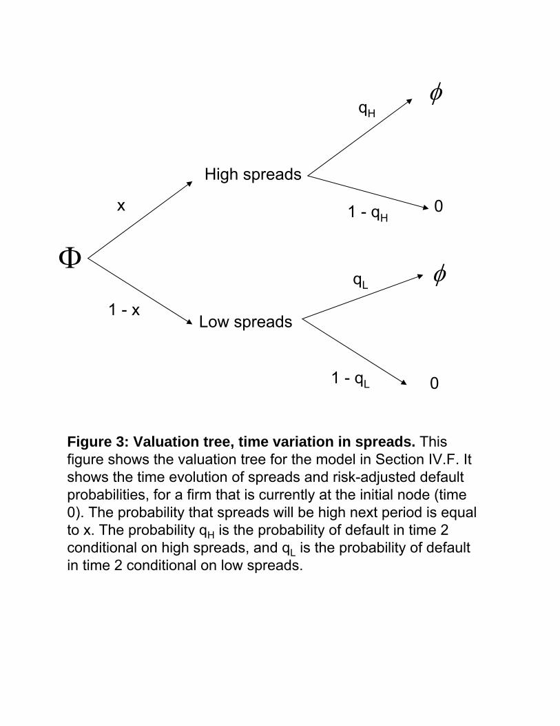
To understand these points more clearly, consider Figure 3. Figure 3 depicts a simple example

that we use to gain some intuition; it is not a full-fledged model. Suppose that there are two

periods, and three dates. We assume that the firm makes its leverage decision at time 0. We must

then compute the NPV of distress costs at that date. At time 1, an aggregate shock is realized,

which affects the market price of risk and the future risk neutral default rates: agents learn that q

is either high, qh, or low, ql. At time 2, financial distress occurs with probability q = qh or ql.

[Insert Figure 3 here]

The first point we want to discuss is the bias from using the historical average instead of the

correct risk neutral average. Let xQ be the risk neutral probability that q jumps to qh at time 1.

The correct ex-ante NPV of financial distress would then be

ΦQ =xQqH +

¡1− xQ

¢qL

(1 + rF )2φ (11)

However, the risk-adjusted valuation that we performed in Section II used historical average spreads

to compute risk-adjusted probabilities of distress. In the example in Figure 3, the naive NPV of

distress using that methodology would be

ΦP =xP qH +

¡1− xP

¢qL

(1 + rF )2φ (12)

16

where xP is the true (historical) probability that q jumps to qh at time 1. In reality, investors are

likely to assign a risk premium to the uncertainty about spreads27. In other words, it is likely that

xQ > xP . In this case, equations (11) and (12) show that our previous calculations underestimate

the true average NPV of financial distress.

The second point that Figure 3 helps clarify is that distress costs depend on the state realized

at time 1. If the firm could adjust its capital structure at time 1, it would make different choices

in the high and low states because the NPV of distress costs is larger in the high state.

Developing a full-fledged model of the time variation in q is beyond the scope of this paper. How-

ever, we feel that it might be useful to have some sense of the potential impact of time variation in

spreads on conditional distress costs. We therefore present some back-of-the-envelope calculations.

As described in Section III.A, we have monthly time-series data from 1985 to 2004 for all ratings

between A and B. We use these data to compute the standard deviation in spreads separately for

each rating and maturity, as a fraction of average 1985-2004 spreads for that rating/maturity. These

ratios range from 50% to 80% for A bonds (depending on maturity), 36% to 70% for BBB bonds,

38% for BB bonds, and 33% for B bonds. We then scale our benchmark average spreads, which

are calculated using 1985-1995 data, uniformly up and down using these ratios. Using these scaled

spreads, we repeat the valuation exercises performed in Sections III.C and III.D.28 We emphasize

that these calculations are only meant as an illustration. In particular, these valuations assume

that the spreads remain indefinitely at the low and high levels.

With these caveats in mind, we find that the NPV of financial distress costs varies substantially

between the high and low scenarios. For example, for BB bonds the NPV of distress goes from

4.73% (low spreads) to 8.38% (high spreads). The impact of time variation on margins, however, is

less clear. For example, the difference in distress costs between A and BBB bonds is highest when

spreads are low. It is equal to 0.89% if spreads are low, and 0.53% when spreads are high. On

the other hand, the difference between A and BB bonds shows the opposite pattern. It is equal to

1.78% when spreads are low, and 3.73% when spreads are high. While these results are suggestive

of the potential effect of time variation in spreads, more research is required to establish their exact

impact on marginal distress costs and capital structure choices.

V. Implications for Capital Structure

17

The existing literature suggests that distress costs are too small to overcome the tax benefits

of increased leverage, and thus that corporations may be using debt too conservatively (Graham,

2000). This quote from Andrade and Kaplan (1998) captures well the consensus view:

“[..] from an ex-ante perspective that trades off expected costs of financial distress

against the tax and incentive benefits of debt, the costs of financial distress seem low [..].

If the costs are 10 percent, then the expected costs of distress [..] are modest because

the probability of financial distress is very small for most public companies.” (Andrade

and Kaplan, page 1488-1489).

In other words, using estimates for φ that are in the same range as those used in Table IV

should produce relatively small NPVs of distress costs because the probability of financial distress

is too low. In this section, we attempt to verify whether this conclusion continues to hold if we

compare marginal, risk-adjusted costs of financial distress to marginal tax benefits of debt.

Naturally, the calculations that we perform in this section are subject to the limitations of the

static trade-off model of capital structure. Our point is not to argue that this model is the correct

one or to provide a full characterization of firms’ optimal financial policies. We simply want to

verify whether the magnitude of the distress costs that we calculate is comparable to that of tax

benefits of debt. To compare the distress costs displayed in Table IV with the tax benefits of debt,

we need to estimate the tax benefits that the average firm can expect at each bond rating. To do

this, we follow closely the analysis in Graham (2000), who estimates the marginal tax benefits of

debt, and Molina (2005), who relates leverage ratios to bond ratings.

A. The Marginal Tax Benefit of Debt

Graham (2000) estimates the marginal tax benefit of debt as a function of the amount of interest

deducted, and calculates total tax benefits of debt by integrating under this function. The marginal

tax benefit is constant up to a certain amount of leverage, and then it starts declining because firms

do not pay taxes in all states of nature and because higher leverage decreases additional marginal

benefits (as there is less income to shield). Essentially, we can think of the tax benefits of debt in

Graham (2000) as being equal to τ∗D (where τ∗ takes into account both personal and corporate

taxes) for leverage ratios that are low enough such that the firm has not reached the point at which

18

marginal benefits start decreasing (see footnote 13 in Graham’s paper). Graham calls this point the

kink in the firm’s tax benefit function. A firm with a kink of 2 can double its interest deductions

and still keep a constant marginal benefit of debt.

In Graham’s sample, the average firm in COMPUSTAT (in the time period 1980-1994) has a

kink of 2.356 and a leverage ratio of approximately 0.34. He estimates that the average firm could

have gained 7.3% of their market value if it had levered up to its kink. In addition, because the firm

remains in the flat portion of the marginal benefit curve until its kink reaches one, these numbers

allow us to compute the implied marginal benefit of debt in the flat portion of the curve (τ∗). If we

assume that the typical firm needs to increase leverage by 2.356 times to move to a kink equal to

one, we can back out the value of τ∗ as 0.157. Tax benefits of debt can then be calculated as 0.157

times the leverage ratio, assuming leverage is low enough that we remain in the flat portion. To the

extent that the approximation is not true for high leverage ratios, we are probably overestimating

tax benefits of debt for these leverage values.29

B. The Relation Between Leverage and Bond Ratings

To compute the tax benefits of debt at each bond rating, we need to assign a typical leverage

ratio to each bond rating. As discussed by Molina (2005), the endogeneity of the leverage decision

affects the relationship between leverage and ratings. In particular, because less risky and more

profitable firms can have higher leverage without greatly increasing the probability of financial

distress, the impact of leverage on bond ratings might appear to be too small.

[Insert Table V here]

The leverage data used in this exercise are reported in Table V. The first column reports Molina’s

predicted leverage values for each bond rating from his Table VI (Molina (2005), p. 1445). Accord-

ing to Molina, these values give an estimate of the impact of leverage on ratings for the average

firm in Graham’s sample. To verify the robustness of our results, we also use the simple descriptive

statistics in Molina’s (2005) Table IV (Molina (2005), p. 1442). Molina’s data, which corresponds

to the ratio of long-term debt to book assets for each rating in the period 1998-2002, are reported

in the second column of Table V. As discussed by Molina, despite the aforementioned endogeneity

19

problem, the rating changes in these summary statistics actually resemble those predicted by the

model. In addition, we report in the third column of Table V the relation between leverage and

ratings that is used by Huang and Huang (2003). These leverage data come from Standard and

Poor’s (1999) and have been used by several authors to calibrate credit risk models (i.e., Cremers

et al., 2005).

C. Tax Benefits versus Distress Costs

Table VI depicts our estimates of the tax benefits of debt for each bond rating. If we use

the leverage ratios from Molina’s (2005) regression model (Panel A), the increase in tax benefits

as the firm moves from the AA to the BBB rating is 2.67%. Under the benchmark valuation of

distress costs (see Table IV), this marginal gain is of a similar magnitude as marginal risk-adjusted

distress costs (2.69% according to Table IV). Analysis of Table IV also shows that the similarity

between marginal tax benefits of debt and marginal financial distress costs holds, irrespective of

our specific assumptions about coupons and recoveries as long as we use the benchmark assumption

of φ = 16.5%.

[Insert Table VI here]

To further compare marginal tax benefits and distress costs, Table VI also reports the difference

between the present value of tax benefits and the cost of distress for each bond rating. Under the

static trade-off model of capital structure, the firm is assumed to maximize this difference. Because

the specific assumption about φ substantially affects marginal distress costs (see Panel B of Table

IV), we report results obtained for φ = 10% and φ = 23%, as well as for the benchmark case of

φ = 16.5%.

Table VI illustrates our conclusion that the distress risk adjustment substantially reduces the

net gains that the average firm can expect from levering up. For example, if φ = 16.5% and we

ignore the risk adjustment (second column), the firm can increase value by 3% to 4% if it levers up

from zero to somewhere around a BBB bond rating. However, once we incorporate the distress risk

adjustment, the net gain from levering up never goes above 1%. The gains from levering up are

higher if φ becomes closer to 10%, as shown in the third and fourth columns. However, the distress

20

risk adjustment substantially reduces the gains from levering up, even for these lower values of φ.

For values of φ closer to 23% (fifth and sixth columns), marginal distress costs are uniformly higher

than marginal tax benefits.

The second, and related, conclusion is that the distress risk adjustment generally moves the

optimal bond rating generated by these simple calculations towards higher ratings. For example,

if φ = 16.5% and we ignore the risk adjustment, a firm should increase leverage until it reaches

a rating of A to BBB, because this rating is associated with the largest differences between tax

benefits and distress costs. However, after incorporating the distress risk adjustment, the difference

becomes essentially flat or decreasing for all ratings lower than AA. Naturally, the result is even

stronger for higher values of φ.

Both conclusions are driven by the finding that marginal risk-adjusted distress costs are very

close to marginal tax benefits of debt. Figure 4 gives a visual picture of these results. In Figure 4 we

plot the difference between tax benefits and distress costs for the benchmark case (φ = 16.5%), both

for non risk-adjusted and risk-adjusted distress costs. Clearly, the marginal gains from increasing

leverage are very flat for any rating above AA if distress costs are risk adjusted. The visual difference

with the inverted U-shape generated by the non risk-adjusted valuation is very clear.

[Insert Figure 4 here]

In Panel B of Table VI, we vary the relationship between leverage and ratings for the benchmark

case of φ = 16.5%. The net gains from levering up are even lower than those in Panel A if we use

Molina’s summary statistics to compute marginal tax benefits of debt (first column). However, if we

use historical probabilities to value financial distress costs, the firm can still gain around 3% in value

by moving from zero leverage to a BBB rating (second column). These gains disappear once distress

costs are risk adjusted (third column). Marginal tax benefits are higher if we use the leverage ratios

from Huang and Huang (fourth column), resulting in large net gains from leverage if distress costs

are not risk adjusted (fifth column). However, the sixth column shows that the difference between

tax benefits and risk-adjusted distress costs is relatively flat, even for these leverage ratios. This

difference increases from 1.73% (AAA rating) to a maximum of 2.26% for the BBB rating. We

conclude that the results are robust to variations in the ratings-leverage relationship.

21

D. Interpretation and Comparison with Previous Literature

Table VI and Figure 4 show that risk-adjusted costs of financial distress can counteract the

marginal tax benefits of debt estimated by Graham (2000). These results suggest that financial

distress costs can help explain why firms use debt conservatively, as suggested by Graham. We

note, however, that Graham’s evidence for debt conservatism is not based solely on the observation

that the average firm appears to use too little debt. His data also show that firms that appear to

have low costs of financial distress have lower leverage (higher kinks). Our results do not address

this cross-sectional aspect of debt conservatism.

Molina (2005) argues that the bigger impact of leverage on bond ratings and probabilities of

distress that he finds after correcting for the endogeneity of the leverage decision can also help

explain why firms use debt conservatively. However, Molina does not perform a full-fledged valu-

ation of financial distress costs, as we have done in this paper. His calculations are based on the

same approximation of marginal costs of financial distress used by Graham (2000), which is to use

Φ = pφ, where p is the 10-year cumulative historical default rate. As we discussed in Section I,

this formula underestimates the NPV of financial distress costs, irrespective of the risk-adjustment

issue.30 Thus, we believe the results on Table VI and Figure 4 provide a more precise comparison

between the NPV of distress costs and the capitalized tax benefits of debt.

VI. Final Remarks

In this paper, we developed a method to estimate the present value of the costs of financial

distress that takes into account the systematic component in the risk of distress. Our formulas

are easy to implement (particularly those in Section I) and should be useful for research and

teaching purposes. We find that the traditional practice of using historical default rates severely

underestimates the average value of distress costs, as well as the effects of changes in leverage on

marginal distress costs. The marginal distress costs that we find can help explain the apparent

reluctance of firms to increase their leverage, despite the existence of substantial tax benefits of

debt.

One caveat is that we risk-adjust distress costs using historical average bond spreads. There

is evidence, however, of significant variation in credit risk premia over time (Berndt et al. (2005),

22

Pan and Singleton (2005)). Time variation in distress costs could lead firms to optimally reduce

their leverage in times when credit spreads are high, as emphasized in the market timing literature.

The large risk adjustments found herein are derived from the significant risk premia that in-

vestors appear to require if they are to hold corporate bonds. These large risk premia might justify

the reluctance of firms to lever up, if their goal is to maximize the wealth of risk-averse investors.

Thus, our results suggest that bond spreads and capital structure decisions are mutually consis-

tent. Considering simultaneously the option market and the bond market, Cremers et al. (2005)

show that the implied volatilities and jump risks implicit in option prices can explain credit spreads

across firms and over time. In other words, they find that corporate bond spreads and option prices

are also mutually consistent. Taken together, these results suggest that market participants, from

options and bonds traders to corporate managers, seem to respond similarly to the market price of

risk.

23

References

Acharya, Viral, Sreedhar Bharath, and Anand Srinivasan, 2005, Understanding the RecoveryRates of Defaulted Securities, Working paper, London Business School and University ofMichigan.

Allen, Linda and Anthony Saunders, 2004, Incorporating Systemic Influences into Risk Measure-ments: A Survey of the Literature, Journal of Financial Services Research, forthcoming.

Altman, Edward, 1984, A Further Empirical Investigation of the Bankruptcy Cost Question,Journal of Finance 39, 1067-1089.

Altman, Edward, Brooks Brady, Andrea Resti, and Andrea Sironi, 2003, The Link between Defaultand Recovery Rates: Theory, Empirical Evidence and Implications, Working paper, New YorkUniversity.

Andrade, Gregor and Steven Kaplan, 1998, How Costly is Financial (not Economic) Distress?Evidence from Highly Leveraged Transactions that Become Distressed, Journal of Finance53, 1443-1493.

Asquith, Paul, Robert Gertner, and David Scharfstein, 1994, Anatomy of Financial Distress: AnExamination of Junk Bond Issuers, Quarterly Journal of Economics 109, 625-658.

Berndt, Antje, Rohan Douglas, Darrell Duffie, Mark Ferguson, and David Schranz, 2005, Mea-suring Default Risk Premia from Default Swap Rates and EDFs, Working paper, CarnegieMelon University and Stanford University.

Blanco, Roberto, Simon Brennan, and Ian Marsh, 2005, An Empirical Analysis of the DynamicRelation between Investment-Grade Bonds and Credit Default Swaps, Journal of Finance 60,2255-2281.

Brennan, Michael and Eduardo Schwartz, 1980, Analyzing Convertible Bonds, Journal of Finan-cial and Quantitative Analysis 15, 907-929.

Chen, Long, David Lesmond, and Jason Wei, 2004, Corporate Yield Spreads and Bond Liquidity,Working paper, Michigan State University and Tulane University.

Chen, Long, Pierre Collin-Dufresne, and Robert Goldstein, 2005, On the Relation Between CreditSpread Puzzles and the Equity Premium Puzzle, Working paper, Michigan State University,U.C. Berkeley, and University of Minnesota.

Collin-Dufresne, Pierre, Robert Goldstein, and Spencer Martin, 2001, The Determinants of CreditSpread Changes, Journal of Finance 56, 2177-2208.

Cremers, Martijn, Joost Driessen, Pascal Maenhout, and David Weinbaum, 2005, IndividualStock-Option Prices and Credit Spreads, Working paper, Yale University, University of Am-sterdam, INSEAD, and Cornell University.

Denis, David and Diane Denis, 1995, Causes of Financial Distress Following Leveraged Recapital-izations, Journal of Financial Economics 37, 129-157.

Driessen, Joost, 2005, Is Default Event Risk Priced in Corporate Bonds?, Review of FinancialStudies 18, 165-195.

24

Duffee, Gregory, 1998, The Relation between Treasury Yields and Corporate Bond Yield Spreads,Journal of Finance 53, 2225-2242.

Duffie, Darrell and Kenneth Singleton, 1999, Modeling Term Structures of Defaultable Bonds,Review of Financial Studies 12, 687-720.

Elton, Edwin, Martin Gruber, Deepak Agrawal, and Christopher Mann, 2001, Explaining theRate Spread on Corporate Bonds, Journal of Finance 56, 247-278.

Fama, Eugene, and Kenneth French, 1989, Business conditions and expected returns on stocksand bonds, Journal of Financial Economics, 23-49.

Fama, Eugene, and Kenneth French, 1993, Common risk factors in the returns on stocks andbonds, Journal of Financial Economics, 3-57.

Feldhutter, Pascal and David Lando, 2005, Decomposing Swap Spreads, Working paper, Copen-hagen Business School.

Franks, Julian and Walter Touros, 1989, An Empirical Investigation of US Firms in Reorganiza-tion, Journal of Finance 44, 747-769.

Gilson, Stuart, 1997, Transaction Costs and Capital Structure Choice: Evidence from FinanciallyDistressed Firms, Journal of Finance 52, 161-196.

Graham, John, 2000, How Big Are the Tax Benefits of Debt?, Journal of Finance 55, 1901-1942.

Hennessy, Christopher and Toni Whited, 2005, Debt dynamics, Journal of Finance 60, 1129-1165.

Huang, Jiang-Zhi and Ming Huang, 2003, How Much of the Corporate-Treasury Yield Spread isDue to Credit Risk?, Working paper, Penn State University and Stanford University.

Jarrow, Robert and Stuart Turnbull, 1995, Pricing Options on Derivative Securities Subject toDefault Risk, Journal of Finance 50, 53-86.

Keim, Donald and Robert Stambaugh, 1986, Predicting returns in the stock and bond markets,Journal of Financial Economics, 17, 357-390.

Lando, David, 2004, Credit Risk Modeling, Princeton University Press.

Leland, Hayne, 1994, Debt Value, Bond Covenants, and Optimal Capital Structure, Journal ofFinance 49, 1213-1252.

Leland, Hayne and Klaus Toft, 1996, Optimal Capital Structure, Endogenous Bankruptcy, andthe Term Structure of Credit Spreads, Journal of Finance 51, 987-1019.

Longstaff, Francis, Eric Neis, and Sanjay Mittal, 2005, Corporate Yield Spreads: Default Riskor Liquidity? New Evidence from the Credit-Default Swap Market, Journal of Finance 60,2213-2253.

Maksimovic, Vojislav and Gordon Phillips, 1998, Asset Efficiency and Reallocation Decisions ofBankrupt Firms, Journal of Finance 53, 1495-1532.

Molina, Carlos, 2005, Are Firms Underleveraged? An Examination of the Effect of Leverage onDefault Probabilities, Journal of Finance 60, 1427-1459.

25

Moody’s, 2002, Default and Recovery Rates of Corporate Bond Issuers - A Statistical Review ofMoody’s Ratings Performance.

Myers, Stuart, 1977, Determinants of Corporate Borrowing, Journal of Financial Economics 5,147-175.

Opler, Tim and Sheridan Titman, 1994, Financial Distress and Corporate Performance, Journalof Finance 49, 1015-1040.

Pan, Jun and Kenneth Singleton, 2005, Default and Recovery Implicit in the Term Structure ofSovereign CDS Spreads, Working paper, MIT and Stanford University.

Saita, Leandro, 2006, The Puzzling Price of Corporate Default Risk, working paper, StanfordUniversity.

Sharpe, Steven, 1994, Financial Market Imperfections, Firm Leverage and the Cyclicality of Em-ployment, American Economic Review 84, 1060-1074.

Shleifer, Andrei and Robert Vishny, 1992, Liquidation Values and Debt Capacity: A MarketEquilibrium Approach, Journal of Finance 47, 1343-1365.

Standard and Poor’s, 1999, Corporate Ratings Criteria.

Titman, Sheridan, 1984, The Effect of Capital Structure on a Firm’s Liquidation Decision, Journalof Financial Economics 13, 137-151.

Titman, Sheridan and Sergey Tsyplakov, 2004, A Dynamic Model of Optimal Capital Structure,Working paper, University of Texas, Austin.

Warner, Jerold, 1977, Bankruptcy Costs: Some Evidence, Journal of Finance 32, 337-347.

Weiss, Lawrence, 1990, Bankruptcy Resolution. Direct Costs and Violation of Priority of Claims,Journal of Financial Economics 27, 255-311.

26

Appendix. Proofs

Proof of Equation (2) in the perpetuity example of Section I: Suppose that the promised return on a perpetualbond is constant over time and that given default creditors recover a fraction of the bond’s market value just priorto default, including the coupons that are due on the year that default occurs. This “recovery of market value”assumption comes from Duffie and Singleton (1999). In addition, we maintain the assumptions that the recovery rateis non-stochastic and that the risk-free rate is constant (equal to rF ).

Let the bond’s promised yearly return be equal to y. Without loss of generality, assume that the bond is pricedat par such that the yearly coupon is also equal to y. Next year, if the bond does not default creditors receive acoupon equal to y. The value of the remaining promised payments is constant over time and equal to one. Thus,creditors receive (1 + y) if there is no default. The recovery of market value assumption implies that creditors willreceive ρ(1 + y) if there is default in year one. Thus, the bond valuation tree is identical to that presented in Figure1, and the bond’s date zero value can be expressed by equation (1). Formula (2) then follows. Q.E.D.

Proof of Equation (8): To understand the recursive formula, consider a two-year bond. If the bond defaults in year1, we have:

EQ£ρ21¤= ρ

£c2 + (1 + c2)B1,2

¤, (A1)

where B1,2 is the date-1 price of a zero that pays one at date 2, and EQ [.] are expectations under the risk-neutralmeasure. If the bond defaults in year 2, we have EQ

£ρ22¤= ρ(1 + c2). We can then write the valuation equation for

a two-period bond as:

V 20 = (1−Q0,1)c2B0,1 +Q0,1ρ

£c2 + (1 + c2)B1,2

¤B0,1 + (A2)

+[(1−Q0,1)(1− q0,2) + (1−Q0,1)q0,2ρ] (1 + c2)B0,2 .

Using the facts that B0,2 = B1,2B0,1, (1 − Q0,1)(1 − q0,2) = (1 − Q0,2), and Q0,1+ (1 − Q0,1)q0,2 = Q0,2, we canrewrite equation (A2) as

V 20 = [(1−Q0,1) +Q0,1ρ]c2B0,1 + [(1−Q0,2) +Q0,2ρ]

¡1 + c2

¢B0,2 . (A3)

Given Q0,1, we can solve equation (A3) for Q0,2. A similar reasoning leads to equation (8). Q.E.D.

Terminal Value calculation (Section III.D): We assume that the marginal, risk-adjusted probability of default isconstant after year 10, that is:

q0,t = q0,10 = 1−(1−Q0,10)(1−Q0,9)

, for t > 10. (A4)

Similarly, we assume that the yearly zero coupon rate is constant after year 10, that is, the yearly risk-free rate afteryear 10 is given by:

rF0,10 =B0,9B0,10

− 1 (A5)

Given these assumptions, we can compute a terminal cost of financial distress at year 10. We can expand equation(5) as:

Φ0 = φ

"10Xt=1

B0,t(1−Q0,t−1)q0,t + (1−Q0,10)q0,11B0,11 + (1−Q0,11)q0,12B0,12 + ...#. (A6)

Using the assumptions that q0,t = q0,10 and rF0,t = rF0,10 for t > 10, we can write:

Φ0 = φ

"10Xt=1

B0,t(1−Q0,t−1)q0,t +B0,10(1−Q0,10)q0,10

q0,10 + rF0,10

#. (A7)

Different Recovery Assumptions (Section IV.B): In addition to assumption 2, the credit risk literature has used thefollowing assumptions about bond recoveries:

27

(i) Recovery of face value (RFV): E(ρtτ ) = E(ρ). This assumption has been used by Brennan and Schwartz (1980)and Duffee (1998). In words, if default occurs at time τ < t, creditors receive a fraction of face value immediatelyupon default. There is zero recovery of coupons.

(ii) Recovery of market value (RMV): E(ρtτ ) = E(ρVtτ ), where V

tτ is the market value prior to default at date τ

of the corporate bond, contingent on survival up to date τ . This assumption comes from Duffie and Singleton (1999).Duffie and Singleton (1999) compare risk-neutral probabilities that are generated by assumptions RMV and RFV,

and find that the two alternative assumptions generate very similar results unless corporate bonds trade at significantpremia or discounts or if the term structure of interest rates is steeply increasing or decreasing. For simplicity, wefocus only on assumption RFV for the robustness checks. Under assumption RFV, E(ρtτ ) = ρ for all τ , t, and thevaluation formula becomes:

V t+10 = ct+1

tXτ=1

(1−Q0,τ )B0,τ + ρt+1Xτ=1

(1−Q0,τ−1)q0,τB0,τ +¡1 + ct+1

¢(1−Q0,t+1)B0,t+1 (A8)

Again, this formula can be easily inverted to obtain Q0,t+1 if one has the sequence {Q0,τ}τ=1..t and the yield on acoupon paying bond with maturity t+ 1. Notice that Q0,0 = 1 and that q0,t+1 = 1− (1−Q0,t+1)

(1−Q0,t) .

28

Endnotes

1. Warner (1977) and Weiss (1990), for example, estimate costs on the order of 3% to 5% offirm value at the time of distress.

2. Altman (1984) reports similar cost estimates of 11% to 17% of firm value three years priorto bankruptcy. However, Andrade and Kaplan (1998) argue that part of these costs might not begenuine financial distress costs, but rather consequences of the economic shocks that drove firmsinto distress. An additional difficulty in estimating ex-post distress costs is that firms are morelikely to have high leverage and to become distressed if distress costs are expected to be low. Thus,any sample of ex-post distressed firms is likely to have low ex-ante distress costs.

3. Structural models in the tradition of Leland (1994) and Leland and Toft (1996) are typicallywritten directly under the risk-neutral measure. Others (e.g., Titman and Tsyplakov (2004), andHennessy and Whited (2005)) assume risk neutrality and discount the costs of financial distress bythe risk-free rate. In either case, these models do not emphasize the difference between objectiveand risk-adjusted probabilities of distress.

4. More precisely, we mean to say that distress tends to occur in states in which the pricingkernel is high. As we discuss in the next paragraph and elsewhere in the paper, there is substantialevidence that default risk has a systematic component.

5. See also Pan and Singleton (2005) for related evidence on sovereign bonds.6. For comparison purposes, the increase in marginal, non risk-adjusted distress costs is only

1.11%.7. This conclusion generally holds for variations in the assumptions used in the benchmark

valuations. The results are most sensitive to the estimate of losses given distress, as we show inSection IV.

8. In a multi-period model, the probability q0,t should be interpreted as the marginal, risk-adjusted default probability in year t, conditional on survival up to year t − 1, and evaluated atdate 0. In this simple example we assume that q0,t = q for all t.

9. See Section III.A for a detailed description of the data.10. This adjustment factor is the historical spread over treasuries on a one-year AAA bond. In

Section III.B we discuss alternative ways to adjust for taxes and liquidity, and we argue that most(but not all) of them imply similar default component of spreads.

11. For simplicity, we use a discrete model in which all payments (coupons, face value, andrecoveries) that refer to year t happen exactly at the end of year t.

12. For example, the average 10+ year spread for BBB bonds in the yield book data is 1.90%for both time periods. Average B-bond spreads are 5.45% if we use 1985-1995 and 5.63% if weuse 1985-2004. In addition, the yield book data and the Huang and Huang data are similar forcomparable ratings and maturities. For example, the 10 year spread for BBB bonds is 1.94% inHuang and Huang.

13. Some average treasury yields that we use are 5.74% (1-year), 6.32% (5-year), and 6.73%(10-year).

14. The default probabilities are calculated using a cohort method. For example, the 5-yeardefault rate for AA bonds in year t is calculated using a cohort of bonds that were initially ratedAA in year t− 5.

15. More specifically, these data refer to cross-sectional average recoveries for original issuespeculative grade bonds.

16. In particular, Huang and Huang’s results imply that the distress probabilities in Leland(1994) and Leland and Toft (1996) incorporate a relatively low risk-adjustment.

17. Chen et al. consider only BBB bonds in their analysis, while Longstaff et al. do not provideestimates for AAA and B bonds. In addition, Huang and Huang (2003) provide estimates for 4-and 10-year maturities only, while Longstaff et al. and Chen et al. consider only one maturity

29

(5-year and 4-year, respectively). Cremers et al. (2005) report 10-year credit spreads for ratingsbetween AAA and BBB.

18. In any case, the difference between 1-year and 4-year AAA spreads (0.04%) is negligible, sousing the 4-year spread would produce virtually identical results.

19. In fact, AAA spreads are very close to the difference between swap and treasury rates (seeFeldhutter and Lando (2005) for some additional evidence on this point). Thus, it is not surprisingthat both methods give similar results.

20. More recently, Saita (2006) also finds high holding period returns and Sharpe ratios forportfolios of corporate bonds.

21. To compute this number, we use the same assumptions about recoveries and risk free ratesthat were used to compute the probabilities in Table III.

22. Notice that equation (5) only requires default probabilities and risk-free rates to translate φestimates into NPV estimates. We assume that the historical marginal default probability is fixedafter year 10 for each rating to compute a terminal value, and we estimate the long-term marginaldefault probability as the average marginal probability between years 10 and 17.

23. Pan and Singleton (2005) use the term structure of sovereign CDS spreads to separatelyestimate risk-neutral recoveries and default intensities and estimate recovery rates that are largerthan the commonly used value of 0.25.

24. Recall, however, that we are also assuming a constant φ. If the reason for a low value of ρin bad times is precisely a high value of φ, then it is less clear that using historical values for ρ andφ leads us to overestimate distress costs.

25. Notice that unlike the robustness checks above, which only affect risk-adjusted probabilities,these variations also impact the valuation using historical probabilities.

26. We thank our referee for suggesting this discussion to us.27. See Pan and Singleton (2005) for evidence on the risk premium associated with time

variation in default probabilities for sovereign bonds.28. In these exercises, we keep all parameters fixed at their benchmark values, including recovery

rates (0.41), losses given distress (0.165), and risk-free rates.29. These tax benefit calculations also ignore risk adjustments. We derived a risk adjustment

in a previous version of the paper, assuming perpetual debt. If D is taken to be the market valueof debt, the risk adjustment does not have a substantial effect on Graham’s formula because it isalready incorporated in D. In fact, with zero recovery rates the interest tax shields are exactlya fraction τ of the cash flows to bondholders in all states, and thus by arbitrage the value of taxbenefits must be exactly equal to τD. With non-zero recovery, there is a risk adjustment thatreduces tax benefits, but it is quantitatively small.

30. In addition, there are two differences between our calculations and those performed byMolina. First, his marginal tax benefits of debt are smaller than those we use because he uses morerecent data from Graham that implies a τ∗ of around 13%. Second, when comparing marginal taxbenefits with marginal costs of distress (Table VII), he uses the minimum change in leverage thatinduces a rating downgrade. In contrast, we use average leverage values for each rating in TableVII.

30

Table I

Term Structure of Yield Spreads This Table gives the spread data used in this study. The spread data for A, BBB, BB and B bonds come from Citigroup’s yieldbook, and refers to average corporate bond spreads over treasuries, for the period 1985-1995. The original data contains spreads for maturities 1-3 years, 3-7 years, 7-10 years and 10+ years for A and BBB bonds. We assign these spreads, respectively, to maturities 2, 5, 8 and 10, and we linearly interpolate the spreads to estimate the maturities that are not available in the raw data. The spreads for BB and B bonds are reported as an average across all maturities. Data for AAA and AA bonds comes from Huang and Huang (2003). The original data contains maturities 4 (1985-1995 averages, from Duffee, 1998), and 10 (1973-1993 averages, from Lehman’s bond index). We linearly interpolate to estimate the maturities that are not available in the raw data.

Ratings

Maturity AAA AA A BBB BB B

1 0.51% 0.52% 1.09% 1.57% 3.32% 5.45%

2 0.52% 0.56% 1.16% 1.67% 3.32% 5.45%

3 0.54% 0.61% 1.23% 1.76% 3.32% 5.45%

4 0.55% 0.65% 1.30% 1.85% 3.32% 5.45%

5 0.56% 0.69% 1.38% 1.94% 3.32% 5.45%

6 0.58% 0.74% 1.28% 1.89% 3.32% 5.45%

7 0.59% 0.78% 1.18% 1.84% 3.32% 5.45%

8 0.60% 0.82% 1.08% 1.79% 3.32% 5.45%

9 0.62% 0.87% 1.20% 1.84% 3.32% 5.45%

10 0.63% 0.91% 1.32% 1.90% 3.32% 5.45%

Table II

Fraction of the Yield Spread Due to Default This Table reports the fractions of yield spreads over benchmark treasury bonds that are due to default, for each credit rating and different maturities. The first column uses Huang and Huang (2003)’s Table 7, which reports calibration results from their model under the assumption that market asset risk premia are counter-cyclically time varying. The second column uses Longstaff et al.’s (2005) Table IV, which reports model-based ratios of the default component to total corporate spread. The third column uses results from Chen et al. (2005). The fraction reported for BBB bonds is the ratio of the BBB minus AAA spread over the BBB minus treasury spread. The fourth column uses results from Cremers et al. (2005). The fractions reported are the ratios between the 10-year spreads in Cremers et al.’s Table 4 (model with priced jumps), and the corresponding 10-year spreads in Table I of this paper. The fifth and sixth columns report for each rating and maturity the ratio between the default component of the spread and the total spread, where the default component is calculated as the spread minus the 1-year AAA spread. The seventh and eight columns report for each rating and maturity the ratio between the default component of the spread and the total spread, where the default component is calculated as the spread minus the difference between swap and treasury rates, for the period 2000-2004. NA = not available.

Huang

and Huang (2003)

Longstaff et al. (2005)

Chen et al. (2005)

Cremers et al. (2005)

Method 1 (AAA spread)

Method 2 (spreads over swaps)

Credit Rating

10-year spread

5-year spread

4-year spread

10-year spread

4-year spread

10-year spread

5-year spread

10-year spread

AAA 0.208 NA 0.000 0.603 0.073 0.190 NA NA

AA 0.200 0.510 NA 0.505 0.215 0.440 NA NA

A 0.234 0.560 NA 0.512 0.609 0.613 0.511 0.570

BBB 0.336 0.710 0.702 0.627 0.724 0.731 0.732 0.729

BB 0.633 0.830 NA NA 0.846 0.846 0.872 0.872

B 0.833 NA NA NA 0.906 0.906 0.916 0.916

Table III Risk Neutral and Historical Default Probabilities

This Table reports cumulative risk-neutral probabilities of default calculated from bond yield spreads, as explained in the text. The Table also reports historical cumulative probabilities of default (data from Moodys, averages 1970-2001), and ratios between the risk-neutral probabilities and the historical ones for 5-year and 10-year maturities. In the last column, we report the average ratio between risk-neutral and historical probabilities across all maturities from 1 to 10.

5-year 10-year

Credit Rating

Historical Risk-Neutral Ratio Historical Risk-Neutral Ratio Average Ratio

AAA 0.14% 0.54% 3.83 0.80% 1.65% 2.07 3.57

AA 0.31% 1.65% 5.31 0.96% 6.75% 7.04 6.22

A 0.51% 7.07% 13.86 1.63% 12.72% 7.80 9.95

BBB 1.95% 11.39% 5.84 5.22% 20.88% 4.00 4.84

BB 11.42% 21.07% 1.85 21.48% 39.16% 1.82 1.86

B 31.00% 34.90% 1.13 46.52% 62.48% 1.34 1.21

Table IV Risk-Adjusted Costs of Financial Distress

This Table reports our estimates of the NPV of the costs of financial distress expressed as a percentage of pre-distress firm value, calculated using historical probabilities (first column), and risk-adjusted probabilities (remaining columns). It also reports in the last row the increase in the NPV of distress costs that is associated with a rating change from AA to BBB. In Panel A we use an estimate for the loss in value given distress of 16.5%. The valuation in the second column (benchmark valuation) assumes recovery of treasury, a recovery rate of 0.41, bond coupons equal to the default component of the yields, and uses method 1 (1-year AAA spread) to calculate the default component of spreads. In the third column we change the recovery rate to 0.25. In the fourth column we use a recovery of face value (RFV) assumption. In the fifth column we assume that coupons are one half times the default component of spreads, and in the sixth column we assume that coupons are one and a half times the default component of spreads. In the seventh column we use Huang and Huang’s (2003) fractions due to default to calculate the default component of spreads. In Panel B we vary the estimate for the loss in value given distress, and report the NPV of distress costs calculated using historical probabilities (first, third and fifth columns), and risk-adjusted probabilities (remaining columns). The risk-adjusted valuations make the same assumptions as the benchmark valuation in Panel A. In the first and second columns we assume a loss given default of 16.5%. In the third and fourth columns we assume a loss given default of 10% and in the fifth and sixth columns we assume a loss given default of 23%.

Panel A (φ = 0.165)

Credit Rating

Historical Benchmark Recovery 0.25

RFV Coupon 0.5*Yield

Coupon 1.5*Yield

Huang and Huang (2003)

AAA 0.25% 0.32% 0.25% 0.31% 0.06% 0.50% 0.49%

AA 0.29% 1.84% 1.47% 1.77% 1.52% 2.07% 0.63%

A 0.51% 3.83% 3.17% 3.66% 3.49% 4.10% 1.14%

BBB 1.40% 4.53% 3.70% 4.24% 4.29% 4.71% 2.28%

BB 4.21% 6.81% 5.59% 6.15% 6.70% 6.88% 5.52%

B 7.25% 9.54% 8.04% 8.44% 9.47% 9.58% 9.15%

BBB minus AA

1.11%

2.69%

2.23%

2.47%

2.77%

2.64%

1.65%

Table IV (cont.) Risk-Adjusted Costs of Financial Distress

Panel B (variations in φ )

φ = 0.165 φ = 0.10 φ = 0.23

Credit Rating

Historical Risk-adjusted

Historical Risk-adjusted

Historical Risk-adjusted

AAA 0.25% 0.32% 0.15% 0.19% 0.35% 0.45%

AA 0.29% 1.84% 0.17% 1.11% 0.40% 2.56%

A 0.51% 3.83% 0.31% 2.32% 0.71% 5.34%

BBB 1.40% 4.53% 0.85% 2.75% 1.95% 6.32%

BB 4.21% 6.81% 2.55% 4.13% 5.87% 9.50%

B 7.25% 9.54% 4.39% 5.78% 10.10% 13.30%

BBB minus AA

1.11%

2.69%

0.67%

1.63%

1.55%

3.75%

Table V

Typical Leverage Ratios for Each Bond Rating This Table reports typical leverage ratios calculated for different bond ratings. The first two columns are drawn from Molina (2005). The first column shows predicted book leverage ratios from Molina’s Table VI. These values are calculated using Molina's regression model (Table V), with values of the control variables set equal to those of the average firm with a kink of approximately two in Graham's (2000) sample. Column II replicates the book leverage ratios in the simple summary statistics of Molina’s Table IV. Column III reports average leverage ratios for firms of a given credit rating, from Huang and Huang (2003). The original source of these data is Standard and Poor’s (1999). Molina (2005)

Credit rating

Summary statistics

Regression model

Huang and Huang (2003)

AAA 9.00% 3.00% 13.08%

AA 17.00% 16.00% 21.18%

A 22.00% 28.00% 31.98%

BBB 28.00% 33.00% 43.28%

BB 34.00% 46.00% 53.53%

B 42.00% 57.00% 65.70%

Table VI Tax Benefits of Debt against Costs of Financial Distress

This Table reports tax benefits of debt and the difference between tax benefits of debt and costs of financial distress. The risk-adjusted valuations assume recovery of treasury, a recovery rate of 0.41, bond coupons equal to the default component of the yields, and uses method 1 (1-year AAA spread) to calculate the default component of spreads. In Panel A, the relation between ratings and leverage is estimated using Molina’s (2005) regression model. This relation is reported in this paper in the first column of Table VI. The first column depicts tax benefits of debt calculated for each leverage ratio as explained in the text. The remaining columns show the difference between tax benefits and distress costs. In the second and third columns we assume that losses given default are equal to 16.5%. In the fourth and fifth columns we assume that losses give default are equal to 10%, and in the sixth and seventh columns we assume a loss given default of 23%. In Panel B, we also report results that obtain when we change the relationship between leverage and bond ratings. The second to fourth columns use Molina’s (2005) summary statistics and the fifth to seventh columns use the relation between leverage and ratings reported by Huang and Huang (2003). We assume a loss given default equal to 0.165 in all calculations reported in Panel B.

Panel A: Predicted Leverage Ratios from Molina (2005)

Tax benefits minus cost of distress

φ = 0.165 φ = 0.10 φ = 0.23

Credit rating

Tax benefits of debt

Historical Risk-adjusted

Historical Risk-adjusted

Historical Risk-adjusted

AAA 0.47% 0.22% 0.15% 0.32% 0.28% 0.12% 0.02%

AA 2.51% 2.22% 0.67% 2.34% 1.40% 2.11% -0.05%

A 4.40% 3.89% 0.56% 4.09% 2.07% 3.69% -0.95%

BBB 5.18% 3.78% 0.65% 4.33% 2.43% 3.23% -1.14%

BB 7.22% 3.01% 0.41% 4.67% 3.09% 1.35% -2.28%

B 8.95% 1.70% -0.59% 4.56% 3.17% -1.15% -4.35%

BBB minus AA

2.67%

Table VI (cont.) Tax Benefits of Debt against Costs of Financial Distress

Panel B: φ = 0.165, Variations in Leverage Ratios

Molina's (2005) summary statistics Huang and Huang (2003)

Tax benefits minus

cost of distress Tax benefits minus

cost of distress

Credit rating

Tax benefits Historical

Risk-adjusted

Tax benefits Historical

Risk-adjusted

AAA 1.41% 1.16% 1.09% 2.05% 1.80% 1.73%

AA 2.67% 2.38% 0.83% 3.33% 3.04% 1.49%

A 3.45% 2.94% -0.38% 5.02% 4.51% 1.19%

BBB 4.40% 3.00% -0.14% 6.79% 5.40% 2.26%

BB 5.34% 1.13% -1.48% 8.40% 4.19% 1.59%

B 6.59% -0.65% -2.95% 10.31% 3.07% 0.77%

BBB minus AA 1.73% 3.47%

Figure 1. Valuation trees, one-period example. This figure shows the trees for the valuations described in Section I.A. Panel A shows the payoff for bond investors, and Panel B shows the deadweight costs of financial distress in default and non-default states. The 1-year risk-adjusted probability of default is equal to q.

A. One-year par bond valuation tree

1

ρ (1+y)

(1+y)

q

1 - q

B. One-year valuation tree for distress costs

0

q

1 - q

Φ

φ

Figure 2: Valuation tree, general model. This figure shows the valuation tree for the model in Section II. It shows the time evolution of deadweight costs of financial distress, for a firm that is currently at the initial node (date 0). The subscripts (0,t) refer to the current date and to a future default date (date t). The probability q0,tis thus the risk-adjusted, marginal probability of default in year t, conditional on no default until year t-1, and evaluated as of date 0.

(1 – q0,1)

q0,2

Prob. surviving beyond year 2 =

(1 – Q0,2) = (1 – q0,1)*(1 – q0,2)

0Φ

1,0φ

2,0φ

3,0φ

….

Prob. default in year 3 = (1 – Q0,2)* q0,3q0,1

q0,3

(1 – q0,2)

(1 – q0,3)

Φ

x

1 - x

High spreads

Low spreads

φ

0

φ

0

qH

qL

1 - qH

1 - qL

Figure 3: Valuation tree, time variation in spreads. This figure shows the valuation tree for the model in Section IV.F. It shows the time evolution of spreads and risk-adjusted default probabilities, for a firm that is currently at the initial node (time 0). The probability that spreads will be high next period is equal to x. The probability qH is the probability of default in time 2 conditional on high spreads, and qL is the probability of default in time 2 conditional on low spreads.

Figure 4: This figure shows the difference between the present value of tax benefits of debt and the NPV of distress costs, expressed as a percentage of pre-distress firm value, as a function of the firm’s bond rating. The upper curve uses the NPV of distress costs calculated with historical probabilities of default, and the lower curve uses the NPV of distress that is calculated with risk-adjusted default probabilities. The present value of tax benefits assumes the marginal tax benefits estimated by Graham (2000), and uses the relation between leverage and bond ratings estimated by Molina (2005).

-1.00%

-0.50%

0.00%

0.50%

1.00%

1.50%

2.00%

2.50%

3.00%

3.50%

4.00%

4.50%

Credit Ratings

Perc

enta

ge o

f Firm

Val

ue

AAA AA A BBB BB B

Risk-adjusted distress costs

Non risk-adjusted distress costs