The Risk Channel of Monetary Policy - IJCB · The Risk Channel of Monetary Policy ... ness of the...

The Risk Channel of Monetary Policy∗

Oliver de Groot Federal Reserve Board

This paper examines how monetary policy affects the riski-ness of the financial sector’s aggregate balance sheet, a mecha-nism referred to as the risk channel of monetary policy. I studythe risk channel in a DSGE model with nominal frictionsand a banking sector that can issue both outside equity anddebt, making banks’ exposure to risk an endogenous choiceand dependent on the (monetary) policy environment. Banks’equilibrium portfolio choice is determined by solving the modelaround a risk-adjusted steady state. I find that banks reducetheir reliance on debt finance and decrease leverage when mon-etary policy shocks are prevalent. A monetary policy reactionfunction that responds to movements in bank leverage or tomovements in credit spreads can incentivize banks to increasetheir use of debt finance and increase leverage, ceteris paribus,increasing the riskiness of the financial sector for the real econ-omy.

JEL Codes: C63, E32, E44, E52, G11.

1. Introduction

The recent financial crisis highlighted the importance of financialintermediaries’ balance sheets, demonstrating that the extent towhich financial intermediaries leverage themselves, and the extent

∗I would like to thank P. Benigno (IJCB co-editor), J. Bianchi, G. Corsetti,E. de Groot, C. Giannitsarou, J. Matheron, M. Paustian, M. Ravn, and J. Robertsfor helpful comments and discussions as well as participants at the Symposiumof the Society of Nonlinear Dynamics and Econometrics, the Federal ReserveBank of Chicago’s Annual Conference on Bank Structures and Competition, theBanque de France–Deutsche Bundesbank Workshop on Current MacroeconomicChallenges, the Federal Reserve Board’s Monetary Analysis Workshop, and theIJCB 2013 Annual Conference. I am also grateful to A. Queralto for makinghis codes available. The views expressed in this paper are those of the authorand do not necessarily reflect those of the Federal Reserve Board. Author e-mail:[email protected].

115

116 International Journal of Central Banking June 2014

to which financial intermediaries make use of debt finance, affectsthe probability of future financial crises occurring and the amount ofdamage a negative shock (either originating in the financial sector ornot) does to the economy. This paper assesses whether the monetarypolicy environment can meaningfully affect financial intermediaries’(privately) optimal mix of outside equity and debt finance and, as aconsequence, their balance sheets’ resilience to shocks.

As the literature on the balance sheet channel has made clear, thefinancial accelerator is greatest when borrowers’ leverage ratios andreliance on debt are high.1,2 Investment banks’ balance sheets in theUnited States in the run-up to the financial crisis displayed these keyindicators of a powerful propagation channel, with historically highleverage ratios and heavy reliance on short-term debt. Quantitativemacroeconomic models have, however, largely remained silent onthe determination of the balance sheet of the financial sector, oftencalibrating the steady state of financial friction models to matchlong-run averages of leverage and short-term debt ratios in the data.In reality, a bank’s balance sheet composition is the product of anoptimizing decision by the bank’s owner(s) in which they face atrade-off between risk and return.

In this paper, I explore a model in which banks face such anoptimizing decision. In particular, this paper is concerned with therole that the design of monetary policy plays in the determinants ofa bank’s balance sheet size and composition.

The design and implementation of monetary policy (as well asregulatory policy) in the run-up to the crisis has received much crit-icism after the event. However, the link between monetary policyand the likelihood or severity of a financial crisis has been diffi-cult to reconcile within standard macroeconomic models. This paperbuilds on the work of Gertler, Kiyotaki, and Queralto (2012), which

1The financial accelerator literature, which has emphasized the balance sheetchannel, can be traced back to Bernanke and Gertler (1989) and Kiyotaki andMoore (1997). The balance sheet channel for banks has been stressed by Gertlerand Kiyotaki (2010) and Gertler and Karadi (2011).

2Several different agency problems have been adopted in the macroeconomicliterature to generate a balance sheet channel. These include costly state veri-fication of borrowers (Townsend 1979 in Bernanke and Gertler 1989), a holdupproblem for lenders (Hart and Moore 1994 in Kiyotaki and Moore 1997), andcoordination failure (Goldstein and Pauzner 2005 in de Groot 2012).

Vol. 10 No. 2 The Risk Channel of Monetary Policy 117

explicitly develops a real business-cycle model in which banks’ bal-ance sheet decisions are endogenously determined. The key innova-tion of this paper is to augment their model with sticky prices tomotivate standard monetary policy objectives. The question is thento ask whether there exists a trade-off between the standard mone-tary policy objectives of a New Keynesian model and the effect theseobjectives may generate on incentives for the endogenous structureof financial institutions’ balance sheets.

To be precise, I present a quantitative New Keynesian business-cycle model in which banks intermediate funds between householdsand non-financial firms. The banks hold a representative asset, whicharises from lending to fund physical capital purchases of the pro-duction sector. Importantly, these assets yield a risky return. Thecomposition of the liability side of the balance sheet is the maininterest in this paper. I assume that banks have three sources offunding available: inside equity (or internal net worth), which is theaccumulation of retained earnings; external equity issuance (out-side equity); and external debt finance (in this case, householddeposits).

The Modigliani and Miller (1958) theorem tells us that in a fric-tionless market, the value of a firm is independent of its capitalstructure. To motivate a trade-off between outside equity and debtfinance, I introduce a simple agency problem that supposes bankershave an incentive to abscond with bank assets, so that at the mar-gin, it is easier for a banker to expropriate funds if outside equityaccounts for a larger share of the bank’s balance sheet. To preventbankers from absconding with assets, households limit the abilityof banks to leverage up their inside equity. However, there is alsoa benefit to the bank of issuing outside equity. If a bank is heav-ily reliant on debt, which is a non-state-contingent claim on thebank, then any fluctuations in the return on assets will have tobe absorbed by the bank’s net worth. Since the return on outsideequity is state contingent and linked to the return on assets, it pro-vides a valuable hedge for banks’ net worth when uncertainty ishigh.

In this framework, the optimal balance sheet composition of thebank will depend on the stochastic nature of asset returns. And oneof the determinants of the stochastic nature of the economy is the


policy environment.3 Banks would like to stabilize volatility in theshadow value of their net worth. If monetary policy acts to achievethis, banks have less incentive to resort to outside equity finance andwill leverage up their balance sheets, thus partly offsetting the aimsof the change in the monetary policy regime. It is this endogenousresponse of the banking system to take on more risk when the assetreturn risk decreases that I refer to as the risk channel of monetarypolicy.

Investigating the endogenous portfolio structure of banks withina quantitative DSGE model is, however, not without its technicalchallenges. The predominant use in the macroeconomic literature ofa first-order approximation around the deterministic steady state isproblematic for what this paper wants to achieve. As is well known,altering the monetary policy rule does not alter the deterministicsteady state of a DSGE model. Nor will it capture banks’ incentiveto alter their steady-state balance sheet composition. To overcomethis problem I solve the model around a risk-adjusted steady state (inthe spirit of Coeurdacier, Rey, and Winant 2011 and Devereux andSutherland 2011, and developed in de Groot 2013), which explic-itly accounts for uncertainty. In a prototypical real business-cyclemodel, this amounts to capturing the effect of household precau-tionary savings on steady-state capital stocks. In the model pre-sented in this paper, the risk-adjusted steady state also capturesthe effect of risk on banks’ steady-state balance sheet composition,which has important implications for the strength of the financialaccelerator mechanism. Computing the risk-adjusted steady stateprovides a challenge precisely because it requires the steady stateand the dynamics of the model around the steady state to be deter-mined jointly. It follows that because the design of monetary policycan alter the risk-adjusted steady state (because of monetary pol-icy’s effect on the second moments of variables in the model), andbecause the altered steady state itself affects the dynamic behaviorof the model around that steady state, we are able to capture therisk channel.

3It is left to future research to incorporate into this framework issues regardingdirect regulation of the financial sector. Focus here is given to the indirect effectstandard monetary policy has on asset returns and the balance sheet decisions ofbanks.


The paper makes two contributions to the literature. First, itshows that exogenous uncertainty (i.e., increases in the standarddeviation of monetary and other shocks) can significantly alterbanks’ (privately) optimal balance sheet composition. Increaseduncertainty reduces the ability of the banking sector to intermediatecredit. Banks’ balance sheets are particularly sensitive to monetaryand capital quality uncertainty because both these shocks have first-order effects on asset returns in the model. Second, the paper showshow the monetary policy regime can also alter the determination ofbanks’ balance sheets. Within a restricted class of monetary policyreaction functions, I find that altering the aggressiveness with whichnominal interest rates react to inflation and output deviations onlyweakly affects the composition of banks’ balance sheet. However, areaction function that responds to deviations of banks’ leverage orcredit spreads can generate significant shifts in the composition ofbanks’ balance sheet and therefore changes in the dynamic responsesto shocks.

Many commentators have put forward the assertion that the con-duct of monetary policy in the late 1990s and early 2000s generateda low-risk environment that incentivized banks to take on more risk,make greater use of short-term debt, and leverage up their balancesheets. More recently, several papers have provided theoretical mod-els for such a risk channel. Chari and Kehoe (2009), Diamond andRajan (2009), and Farhi and Tirole (2012), among others, focus onthe moral hazard consequences of bailouts and credit market instru-ments. Farhi and Tirole (2012)’s paper, for example, considers athree-period endowment economy with strategic complementaritiesbetween private leverage and monetary policy. When maturity trans-formation is prevalent, the central bank has little choice but to facili-tate refinancing. Equally, reducing private leverage lowers the returnon equity. The key insight of this literature is that banks choose tocorrelate their risk exposures, that optimal monetary policy can betime inconsistent, and that macroprudential policy can therefore bewelfare enhancing. Diamond and Rajan (2009), using a similar three-period endowment environment, also show that monetary policy istime inconsistent. Lowering interest rates when households demandfunds prevents a damaging run on illiquid assets, but encouragesbanks to increase leverage and fund more illiquid projects. Optimalmonetary policy under commitment in their environment involves


raising interest rates when there is no liquidity crisis in order topunish banks that have chosen to be illiquid.

There is also a growing literature on macroprudential policyincluding, among others, Lorenzoni (2008), Nikolov (2010), Bianchi(2011), Korinek (2011), and Stein (2012). Lorenzoni (2008), forexample, is another three-period model with financial frictions, vialimited commitment in financial contracts, which results in exces-sive borrowing ex ante and excessive volatility ex post. The frictiongenerates a pecuniary externality that is not internalized in privatecontracts and provides a framework to evaluate policies to preventfinancial crises. While providing important insights, most of thesemodels are not rich enough to provide quantitative insights into theimportant trade-offs policymakers may face.

The key extension of this paper, therefore, is that it studies therisk taking of banks within a quantitative macroeconomic modelwith nominal frictions, allowing for the joint examination of mone-tary policy design and banks’ balance sheet composition. The paperproceeds as follows: Section 2 presents the model. Section 3 sets outthe parameterization and explains the solution technique. Section 4presents the results of the numerical experiments, and section 5concludes.

2. Model

The baseline model is a DSGE model with investment costs, nomi-nal rigidities, and financial frictions. There are five types of agents:households, capital producers, manufacturers, retailers, and bankers.The banking sector follows Gertler, Kiyotaki, and Queralto (2012).In particular, banks intermediate funds between households andmanufacturers by raising both debt and (outside) equity. An agencyproblem between households and banks, however, limits how muchbanks are able to leverage their (inside) equity. The model is closedwith a monetary policy reaction function. Of central interest to thispaper is the interaction between the monetary policy environmentand banks’ endogenous balance sheet composition.

2.1 Households

There is a unit measure of identical households. Each householdconsists of a fraction 1 − f of bankers and f of workers. Workers


supply labor to manufacturers and bring home wages to their house-hold. Bankers manage banks and bring home any earnings. Withineach family, there is consumption insurance. Workers and bankersrotate over time, with a banker becoming a worker with fixed prob-ability 1 − θ. As (1 − θ)f bankers become workers, a proportion(1 − θ)f/(1 − f) of workers become bankers, keeping the size of thetwo populations unchanged. The household provides its new bankerswith a small startup fund.

Household preferences are given by

maxEt

∞∑

i=0

βi 11 − ζ

(

Ct+i − hCt+i−1 − �

1 + ϑL1+ϑ

t+i

)1−ζ

, (1)

where Et(.) denotes the rational expectations operator, conditionalon the time t information set; β ∈ (0, 1) is the subjective discountfactor; Ct is consumption; and Lt is labor supply. The followingparameter restrictions ensure well-behaved preferences: h ∈ [0, 1),�, ϑ > 0.

Households have access to two financial assets: bank debt(deposits), Dt, and bank (outside) equity, Et, at relative priceQE,t−1. Bank debt pays the non-state-contingent (risk-free) grossreal return Rt from t − 1 to t while bank equity pays a state-contingent gross real return, denoted RE,t. Let Wt be the real wageand Υt net payoffs to the household from ownership of financial andnon-financial firms. The household budget constraint is given by

Ct = WtLt + Υt + RtDt + QE,t−1RE,tEt − Dt+1 − QE,tEt+1. (2)

The household’s first-order optimality conditions are given by

Wt = −UL,t

UC,t, Et (Λt,t+1) Rt+1 = 1 and Et (Λt,t+1RE,t+1) = 1,

(3)

where

Λt−1,t ≡ βUC,t

UC,t−1

denotes the stochastic discount factor between periods t − 1 and t,and UC,t and UL,t denote the marginal utility of consumption andthe marginal (dis)utility of labor, respectively.


2.2 Manufacturers

A representative, perfectly competitive manufacturer produces inter-mediate goods that are sold to retailers. At the end of period t,the manufacturer purchases capital, Kt+1, at price QK,t for use inproduction in period t + 1. The manufacturer purchases the capi-tal using funds from banks. By assumption, there is no friction inthe process of obtaining funds from banks, and the manufacturer istherefore able to offer the bank a state-contingent security. In thisregard, the banks are like private equity funds. Let εA,t and εK,t

denote total factor productivity and capital quality, respectively. Ateach time t, the manufacturer uses capital and labor to produceoutput, Yt:

Yt = exp (εA,t) (exp (εK,t) Kt)α

L1−αt , (4)

where α ∈ (0, 1). εA,t and εK,t are exogenous stochastic processes ofthe form εs,t+1 = ρsεs,t + ηsεs,t+1 for s = (A, K) and εs,t+1 ∼Niid(0, 1). Let Xt = Pm,t

Ptbe the ratio of the price of inter-

mediate goods, Pm,t, to the aggregate price level, Pt. The man-ufacturer’s first-order optimality condition for labor demand isgiven by

Wt = Xt (1 − α)Yt

Lt. (5)

Since manufacturers are perfectly competitive, the gross real returnon capital is

RK,t = exp (εK,t)Xtα

Yt

exp(εK,t)Kt+ (1 − δ) QK,t

QK,t−1. (6)

2.3 Capital Producers

At the end of period t, competitive capital producers buy the entirecapital stock from manufacturers, repair depreciated capital, andbuild new capital. Production of capital involves convex adjustmentcosts. The capital producers then sell both the repaired and new


capital back to manufacturers. The objective of a capital produceris given by

maxEt

∞∑

i=0

Λt,t+i

(

QK,t+iIt+i −(

1 +ϕI

2

(

It+i

It+i−1− 1

)2)

It+i

)

,

(7)

where It is investment and ϕI ≥ 0 scales the adjustment costs. Thecapital producer’s first-order optimality condition determines theprice of capital:

QK,t = 1 +ϕI

2

(

It

It−1− 1

)2

+(

It

It−1

)

ϕI

(

It

It−1− 1

)

− EtΛt,t+1

(

It+1

It

)2

ϕI

(

It+1

It− 1

)

. (8)

The aggregate capital stock in the economy evolves according to

Kt+1 = (1 − δ) exp (εK,t) Kt + It. (9)

2.4 Retailers

Final output, Yt, is a CES aggregator of measure one of differentiatedretailers

Yt =(∫ 1

0Y

ε−1ε

r,t dr

)ε

ε−1

, (10)

where Yr,t is the output of retailer r and ε > 1 denotes the intratem-poral elasticity of substitution across different varieties of retailgoods. From cost minimization of users of final output,

Yr,t =(

Pr,t

Pt

)−ε

Yt and Pt =(∫ 1

0P 1−ε

r,t dr

)1

ε−1

. (11)

Retailers costlessly brand intermediate output: One unit of interme-diate output is used for one unit of retail output. Retailers enjoymonopolistic pricing power but face a convex price adjustment cost


(a la Rotemberg 1982), which generates nominal rigidities in theeconomy. The objective of retailers is given by

maxEt

∞∑

i=0

Λt,t+i

×(

Pr,t+i

Pt+iYr,t+i − Xt+iYr,t+i − ϕΠ

2

(

Pr,t+i

Pr,t+i−1Π− 1

)2

Yt+i

)

,

(12)

where Π is the steady-state gross inflation rate and ϕΠ ≥ 0 scalesthe adjustment costs. Noting that the equilibrium will be symmetric(Pr,t+i = Pt+i) for all r and i, the retailers’ first-order optimalitycondition is given by

ϕΠ

(

Πt

Π− 1

)

Πt

Π

= 1 − ε (1 − Xt) + ϕΠEt

(

Λt,t+1

(

Πt+1

Π− 1

)

Πt+1

ΠYt+1

Yt

)

,

(13)

where Πt is the gross inflation rate from t − 1 to t.Since price adjustment and investment adjustment costs are paid

in real units, the economy’s aggregate resource constraint is given by(

1 − ϕΠ

2

(

Πt

Π− 1

)2)

Yt = Ct +

(

1 +ϕI

2

(

It

It−1− 1

)2)

It. (14)

2.5 Banks

The model thus far is a conventional DSGE model. Frictionlessfinancial intermediation would ensure that the following arbitragecondition should hold:

EtΛt,t+1 (RK,t+1 − Rt+1) = 0.

Instead, this section develops a model of banking with agency prob-lems, driving a wedge between EtΛt,t+1RK,t+1 and EtΛt,t+1Rt+1,


and ensuring a non-trivial role for the composition of banks’ balancesheets for economic outcomes.

Banks lend funds, obtained from households, to manufacturers.Bank j’s balance sheet is

QK,tKj,t+1 = Nj,t + Dj,t+1 + QE,tEj,t+1,

where Kj,t+1 is the quantity of financial claims on manufacturers’gross returns on capital. Since these claims are perfectly state con-tingent, it is possible to denominate one claim as one unit of capital,as I have done, implying that QK,t is also the relative price of eachclaim. Nj,t is the amount of net worth—or inside equity—that abank has and Dj,t+1 the deposits that the bank obtains from house-holds. Ej,t+1 is the quantity of outside equity that the bank issuesto households and QE,t is the relative price of each claim. If one unitof outside equity is the claim on one unit of capital, then the grossreal return on outside equity is given by

RE,t = exp (εK,t)Xtα

Yt

exp(εK,t)Kt+ (1 − δ) QE,t

QE,t−1.

The bank’s inside equity evolves as the difference between earn-ings on assets and payments on liabilities,

Nj,t+1 = (RK,t+1 − RE,t+1Bj,t − Rt+1 (1 − Bj,t)) QK,tKj,t+1

+ RtNj,t,

where Bj,t ≡ QE,tEj,t+1QK,tKj,t+1

. Bank assets earn the state-contingent realgross return RK,t+1. Household deposits get paid the non-contingentreal gross return Rt+1 and outside equity is paid the state-contingentreal gross return RE,t+1. The bank’s objective is given by

Vj,t = maxEt

∞∑

i=0

(1 − θ) θiΛt,t+1+iNj,t+1+i. (15)

To motivate a limit on a bank’s ability to expand its balancesheet, I follow Gertler, Kiyotaki, and Queralto (2012) by introduc-ing a moral hazard problem: Bankers are able to abscond with a


fraction, Θ, of bank assets. This introduces an incentive compatibil-ity constraint:

Vj,t ≥ Θ (Bj,t) QK,tKj,t+1. (16)

Households will only provide funds up to the point at which bankersare still marginally better off by not absconding with assets. To moti-vate a non-trivial choice for the composition of bank’s liabilities,I assume that the fraction of bank assets that bankers can abscondwith is convex in the share of assets funded by outside equity:

Θ (Bj,t) = κ0

(

1 + κ1Bj,t +κ1

2B2

j,t

)

. (17)

The rationale, that it is more difficult to abscond with assetsfunded by debt than by equity, comes from Calomiris and Kahn(1991) and relies on the insight that debt requires the bank to meeta non-contingent payment every period, while dividend paymentson equity are tied to the performance of the banks’ assets and aretherefore more difficult to monitor by outsiders.4

We can express Vj,t as follows:

Vj,t = (μK,t + Bj,tμE,t) QK,tKj,t+1 + μN,tNj,t (18)

with

μK,t = Et (Λt,t+1Ωt+1 (RK,t+1 − Rt+1)) (19)

μE,t = Et (Λt,t+1Ωt+1 (Rt+1 − RE,t+1)) (20)

μN,t = Et (Λt,t+1Ωt+1) Rt+1, (21)

where Ωt = (1 − θ) + θBtφt. I assume that, in equilibrium, theincentive compatibility constraint, equation (16), binds.5 Rewriting

4If Θ was independent of B, banks would strictly prefer to issue outside equityover debt. In this case, with outside financing coming from only equity, banks’ networth would be completely shielded from movements in assets returns, thus ren-dering the financial accelerator obsolete. There would, however, remain a creditspread in steady state that cannot be arbitraged away.

5I choose parameter values such that, within the neighborhood of the steadystate, the incentive compatibility constraint does, in fact, bind.


equation (16) gives an expression for the inverse of the ratio of insideequity to total assets

φj,t =μN,t

Θ (Bj,t) − (μS,t + Bj,tμE,t),

where φj,t ≡ QK,tKj,t+1Nj,t

. Combining the first-order conditions of thebank’s objection function, equation (15), subject to the incentivecompatibility constraint, equation (16), for Kj,t+1 and Bj,t givesthe following equilibrium condition:

μE,t

(μK,t + Bj,tμE,t)=

Θ′ (Bj,t)Θ (Bj,t)

. (22)

Symmetry of the equilibrium ensures that Bj,t = Bt and φj,t =φt for all j. New banks receive a startup fund from households ofωQK,tKt. The evolution of aggregate net worth is therefore given by

Nt+1 = θ ((RK,t − RE,tBt−1 − Rt (1 − Bt−1)) φt−1 + Rt) Nt

+ ωQK,tKt.

2.6 Monetary Policy

Monetary policy is characterized by a simple reaction function

(

RN,t

RN

)

=((

Πt

Π

)χΠ(

Xt

X

)χX(

φt

φ

)χφ

exp (χS (St − S)))1−χRN

×(

RN,t−1

RN

)χRN

exp (εM,t) (23)

with the nominal interest rate, RN,t, reacting only to deviations ofobservable variables from their respective steady states (denoted byvariables without time subscripts). In this setup, the central bankuses Xt as an observable proxy of the output gap. The reactionfunction allows for the possibility that monetary policy reacts totwo financial indicators, bank leverage and the credit spread, St ≡EtRK,t+1 − Rt+1. Monetary policy shocks follow the exogenous sto-chastic process εM,t+1 = ρMεM,t+ηMεM,t+1 with εM,t ∼ Niid(0, 1).


Finally, the link between nominal and real interest rates is given bythe Fisher relation:

RN,t = Rt+1Et (Πt+1) . (24)

2.7 Discussion of the Model

The banking sector—and, in particular, banks’ balance sheetcomposition—in section 2 is of primary interest in this paper; therest of the model is relatively standard.

To understand the relationship between the monetary policyenvironment and the composition of banks’ balance sheets, consideran expansionary monetary policy shock. Nominal rigidities in theeconomy means that a fall in the nominal risk-free rate generates afall in the real risk-free rate. In a model without financial frictions,arbitrage ensures that the required expected return on capital falls(to first order) one-for-one with a fall in the risk-free rate. Since thereare diminishing marginal returns to capital, a fall in the requiredexpected return on capital means that a larger set of investmentprojects have a positive net present value, generating a boom ininvestment.6

The existence of an agency problem limits the amount of credithouseholds are willing to extend as a function of banks’ net worth,as an overextension of credit could mean that bankers have an incen-tive to forgo their accumulated retained earnings and abscond witha fraction of the banks’ assets instead. The limit on the creation ofcredit prevents arbitrage, thus driving a wedge between the expectedrequired return on capital and the risk-free rate.

When banks’ asset returns are below expectation, banks use theirretained earnings to pay their creditors. The fall in banks’ net worththerefore heightens the agency problem, causing the wedge betweenthe expected required return on capital and the real risk-free rateto move countercyclically While in a frictionless financial sector theexpected required return on capital and the risk-free rate move one-for-one, in the model with an agency problem the expected requiredreturn on capital moves by more than one-for-one. As a consequence,

6For simplicity in this discussion, I abstract from changes in other relativeprices, like wages and the effect on the labor market outcomes.


in response to an expansionary monetary policy shock, an evenlarger set of investment projects have a positive net present value,generating an even greater boom in investment.

The extent to which banks are able to leverage themselves, andthe extent to which banks’ net worth is damaged by shocks, is crucialfor the amplification and propagation of shocks through the financialsystem. In particular, a bank heavily funded with non-contingent lia-bilities (debt) will experience high volatility in its net worth, whilefor a bank that issues a lot of outside equity, a state-contingent claimon the bank, unexpected movements in asset returns are absorbedby the concomitant movement in the return paid on outside equity,thus damping fluctuations in net worth.

This begs the question, why don’t banks issue only state-contingent claims? The insight from Calomiris and Kahn (1991),is that debt is a disciplining device for bankers. Banks, in choosingtheir (privately) optimal mix of short-term debt and outside equityfinance, are therefore an endogenous source of the amplification andpropagation of shocks in the economy.

The banker maximizes the value of his or her bank, V, subject tothe incentive constraint binding. Given the net worth of the bank,the banker has two choice variables: the quantity of assets (capital)it invests in, QK,tKt+1, and the share of those assets funded by issu-ing outside equity, Bt. The marginal benefit of an additional unit ofoutside equity is given by μE,tQK,tKt+1, while the marginal benefitof an additional asset is μK,t + μE,tBt. Thus, the marginal rate ofsubstitution between outside equity and expanding the size of thebalance sheet is −μE,tQK,tKt+1

μK,t+μE,tBt. The unconstrained optimum for the

bank, all else equal, is to choose the highest feasible leverage and toraise external funds using only outside equity.

From the incentive compatibility constraint, the price of an addi-tional unit of outside equity is

(

dΘt

dBt−μE,t

)

QK,tKt+1, while the priceof an additional asset is Θt − (μK,t + μE,tBt). Both these prices areassumed positive. The first says that substituting debt with an addi-tional unit of outside equity causes the ratio of assets that can beexpropriated to rise more than the value of the bank, causing theconstraint to tighten. The second says something similar, that anadditional asset will raise the marginal quantity of assets that canbe expropriated more than it raises the value of the bank, again


causing the constraint to tighten. The marginal rate of transforma-tion between outside equity and an additional asset is therefore

dφ

dB= − Θ′ − μE

Θ − (μK + μEB)φ < 0, (25)

where Θ′ refers to the first derivatives of equation (17) with respectto B. The marginal rate of transformation is strictly negative. Inother words, the banker faces a trade-off since an increase in outsideequity issuance must result in a lower capital-to-net-worth ratio,all else equal. Equating the marginal rate of substitution and themarginal rate of transformation delivers the equilibrium relation ofequation (22).

In a risk-free environment, the benefit of substituting outsideequity for debt is zero (μE = 0), since the return on debt and out-side equity is identical (R = RE). In addition, it follows that Θ′ = 0.We can show the following comparative statics in the neighborhoodof the deterministic steady state:

dBdμE

= Θ−BΘ′

Θ′′(μK+μEB)dBdμE

∣

∣

∣

μE=0= Θ

Θ′′μK> 0

dBdμK

= Θ′

μEΘ′−Θ′′(μK+μEB)dB

dμK

∣

∣

∣

μE=0= 0

. (26)

The relations in the first line hold because Θ is convex by assump-tion. Thus, a marginal increase in the value of outside equity leadsto an increase in the share of outside equity issuance. The secondline says that, at the margin, an increase in the excess value of assetsover deposits does not generate any portfolio shifting.

dφdμE

= BφΘ−(μK+μEB) − Θ′−μE

Θ−(μK+μEB)φdx

dμE

dφdμE

∣∣∣μE=0

= BφΘ−(μK+μEB) > 0

dφdμK

= φΘ−(μK+μEB) − Θ′−μE

Θ−(μK+μEB)φdx

dμK

dφdμK

∣∣∣μE=0

= φΘ−(μK+μEB) > 0

dφdμN

= 1Θ−(μK+μEB) − Θ′−μE

Θ−(μK+μEB)φdx

dμN

dφdμN

∣∣∣μE=0

= 1Θ−(μK+μEB) > 0

(27)

The above comparative statics make use of the binding incentivecompatibility constraint. The effect on leverage of a change in μE ,μK , or μN is the outcome of a direct and an indirect effect, as a result


of a change in the liability mix of the bank. In the neighborhood ofthe deterministic steady state, the indirect effect is zero.

To understand how risk affects this equilibrium relationship, weneed to interpret μE,t and μK,t. μE,t is the excess value of substi-tuting outside equity for deposits while μK,t is the excess value ofassets over deposits and μK,t + μE,tBt is the excess value of assetsover external finance:

μE,t ≡ Et (Λt,t+1Ωt+1 (Rt+1 − RE,t+1)) (28)

μK,t + μE,tBt ≡ Et (Λt,t+1Ωt+1 (RK,t+1 − Rt+1 (1 − Bt)

−RE,t+1Bt)) . (29)

Clearly, both μE,t and μE,t + μE,tBt need to be non-negative forthe banker’s problem to be well defined. Notice also that both equa-tions look like asset-pricing equations, where the left-hand side is theprice, Λt,t+1Ωt+1 is the stochastic discount factor, and the remain-der of the right-hand side is the expected return. We can interpret˜Λt+1 ≡ Λt,t+1Ωt+1 as the banker’s stochastic discount factor, whichis different from the household’s stochastic discount factor, Λt,t+1.Ωt+1 is the shadow marginal value of a unit of net worth. Ωt+1varies countercyclically because the incentive constraint becomesmore binding in a downturn. Thus, the bankers’ stochastic discountfactor is countercyclical and more volatile than the household’s sto-chastic discount factor.

To be clear, I compare equation (28) to the first-order con-ditions of the household’s problem (equations in (3)), which give0 = Et(Λt,t+1(Rt+1−RE,t+1)). At this stage, it is useful to introducethe concept of the risk-adjusted steady state. As discussed earlier, atthe deterministic steady state, bankers and households are indiffer-ent between holding debt and outside equity. To ensure a determi-nate portfolio choice, we must consider a steady state that accountsfor future uncertainty. The risk-adjusted steady state is defined asthe portfolio that agents would hold if there was no risk today (thevector εt = 0) but they expected risk in the future (εt+τ = Niid(0, I)for all τ > 0). To compute the risk-adjusted steady state, it is possi-ble to take a second-order approximation around the point εt+1 = 0,which gives

0 = Λ (R − RE) − covt (Λt,t+1, RE,t+1) (30)

μE = ˜Λ(R − RE) − covt(˜Λt+1, RE,t+1), (31)


where variables without time subscripts denote the variables attheir risk-adjusted steady state and covt(Λt,t+1, RE,t+1) is a covari-ance term conditional on time t information. Clearly, incorporat-ing expected risk at the risk-adjusted steady state allows monetarypolicy to affect steady-state portfolio choices because the conductof monetary policy can affect how variables co-move in the econ-omy.

It follows that because covt(Λt,t+1, RE,t+1) and covt(˜Λt+1,RE,t+1) are both negative, but with the second larger than the first,and with Ω > 0, the excess marginal value of substituting outsideequity for debt for the banker is positive, μE > 0. In other words,increased volatility in the return on outside equity makes bankersmore willing to issue outside equity, causing the excess marginalvalue of substituting outside equity for debt to rise. Moreover, whilethe credit spread may rise in a high-uncertainty state, banks’ dis-counted value of that credit spread, μK,t, falls. This is because therealized spread between the return on capital and the cost of bor-rowing is procyclical. When μK,t+μE,tBt falls, the value of the bankis lower, as is the maximum leverage ratio that it can attain.

In section 4 I validate this discussion by conducting numericalexperiments to show how banks’ balance sheet compositions areaffected by the policy environment in which banks operate.

3. Parameterization and Solution Technique

3.1 Parameterization

Table 1 summarizes the structural parameter values used in thenumerical experiments that follow. Many of the parameters are con-ventional in the literature—such as the income share of capital, α;the subjective discount factor, β; and the depreciation rate, δ—andall are set consistent with time periods denoting quarters. House-hold preferences display habit formation and abstract from wealtheffects on labor supply. The habit parameter, h = 0.75, is set towardsthe upper end of the range of values seen in the literature. ζ = 2implies (holding hours constant) an intertemporal elasticity of sub-stitution of 0.5. ϑ = 0.33 implies a Frisch elasticity of labor supplyof 3. The weighting term, � = 0.25, ensures that households allocate20 percent of their time to work (at the deterministic steady state).


Table 1. Parameterization

Description Value

Standard DSGE Parameters

α Income Share of Capital 0.33β Quarterly Subjective Discount Rate 0.99

h, ζ, �, ϑ Preferences 11−ζ

(Ct − hCt−1 − �

1+ϑL1+ϑ

t

)1−ζ0.75, 2, 0.25, 0.33

ε Price Elasticity of Demand 4.17δ Quarterly Depreciation Rate 0.025ϕΠ Adjustment Cost ϕΠ

2 (Πt/Π − 1)2 48.8ϕI Adjustment Cost ϕI

2 (It/It−1 − 1)2 1

Banking Sector

θ Survival Probability 0.9685κ0, κ1, κ2 Agency Cost: κ0

(1 + κ1B + κ2

2 B2)

0.26, −0.75, 8.35ω Transfer to New Bankers 0.0289

Exogenous Shock Processes

ρA, 100ηA Technology Shock 0.95, 0.45ρK , 100ηK Capital Quality Shock 0, 1.5ρM , 100ηM Monetary Policy Shock 0.15, 0.24

Monetary Policy

χΠ, χX , χRNStandard Monetary Policy Parameters 1.5, 0.5/4, 0

χφ, χS Leverage, Credit Spread 0, 0

I follow Gertler and Karadi (2011) in choosing ε = 4.17 for the priceelasticity of demand. Following Keen and Wang (2007), I choosethe Rotemberg price adjustment parameter, ϕΠ, to match a Calvo(1983)-style model in which firms face a 0.779 probability of keepingprices fixed every quarter. The investment adjustment parameter isset at 1.

The four parameters novel to the banking sector’s agency prob-lem are calibrated to match the same steady-state moments as thosein Gertler, Kiyotaki, and Queralto (2012). In particular, they matcha credit spread of 120 basis points, a ratio of total equity to assets,B+1/φ = 1/3, and a ratio of inside to outside equity of 2/3. Finally,they ensure that a rise in the standard deviation of capital qualityinnovations from 0.69 percent to 2.07 percent reduces the inverse


of the total-equity-to-asset ratio by 1/3. My method of solving forthe risk-adjusted steady state differs from the method preferred byGertler, Kiyotaki, and Queralto (2012), thus implying a need forthe parameters of the banking sector to be recalibrated from thosein Gertler, Kiyotaki, and Queralto (2012). In particular, the riskadjustment in my solution method is smaller for a given standarddeviation of the exogenous shock process. Thus, the key differenceis that my κ2 = 8.35 as opposed to 13.4.7 The smaller value of thisparameter means that the incentive compatibility constraint tight-ens less in my model for a given change in the outside-equity-to-assetratio.

The model has three exogenous stochastic processes. The capitalquality shock is calibrated in line with Gertler, Kiyotaki, and Quer-alto (2012). In the baseline, I set ηK = 1.5 percent and ρK = 0.The technology shock is considered to be highly persistent, withthe ρA = 0.95. The monetary policy persistence parameter is lower,ρM = 0.15. In the baseline, the standard deviations of the two shocksare ηA = 0.46 percent and ηM = 0.24 percent, respectively.

The baseline reaction function is fairly conventional, with thefeedback coefficient on inflation and output set at 1.5 and 0.5/4,respectively.

3.2 Solution Technique

The aim is to find a first-order approximation of the model’s dynam-ics in the neighborhood of a risk-adjusted steady state. A formalstatement of the solution technique is presented in appendix 1. HereI provide a description of the technique using a prototypical realbusiness-cycle model. In so doing, I explain how the solution tech-nique compares to others in the literature.

7κ1 is negative in the calibration. This means that even in the determinis-tic steady state, banks issue a non-zero amount of outside equity. The economicrationale might be that there are some efficiency gains in monitoring the bankby having at least a small proportion of banks’ funding coming from outsideequity. More importantly, though, the share of outside equity to assets respondsto shocks. Therefore, the calibration of κ1 and the standard deviation of shocksare chosen to ensure that the first-order approximation of the model does notgenerate outside equity turning negative.


Consider the prototypical real business-cycle model with equilib-rium conditions,8

Etβ

(

Ct+1

Ct

)−ζ

α exp (ηAεA,t+1) Kα−1t = 1 (32)

exp (ηAεA,t) (Kt)α − Kt+1 = Ct, (33)

the exact solution of which is given by the decision rules, Ct =g(Kt, ηAεA,t) and Kt+1 = h(Kt, ηAεA,t). Since g and h do not,in general, have a closed-form representation, we wish to find afirst-order approximation of the functions g and h around the risk-adjusted steady state

Ct − C = gK (K, 0) (Kt − K) + gε (K, 0) ηAεA,t (34)

Kt+1 − K = hK (K, 0) (Kt − K) + hε (K, 0) ηAεA,t, (35)

where C and K without time subscripts denote the risk-adjustedsteady-state values of consumption and capital, respectively, andgK , gε, hK , hε are, as yet, undetermined coefficients. Note, though,that the first-order coefficients are a function of the steady state, K.

Following Coeurdacier, Rey, and Winant (2011), the risk-adjusted steady state is defined as the “point where agents chooseto stay at a given date if they expect future risk and if the real-ization of shocks is 0 at this date.” This implies setting Ct = C,Kt+1 = Kt = K, and εA,t = 0 in (32) and (33). The realizationof Ct+1 and εA,t+1 are unknown at date t. Substituting equation(34) into equation (32) leaves only the exogenous stochastic variable,εA,t+1:

αβ1

C−ζKα−1Et {C + gε (K, 0) ηAεA,t+1}−ζ exp (ηAεA,t+1) = 1.

We need to evaluate the object

Et {C + gε (K, 0) ηAεA,t+1}−ζ exp (ηAεA,t+1) ,

8This model is nested within the full model presented in section 2. Finan-cial and nominal frictions have been removed. Households are assumed to sup-ply a fixed quantity of labor, normalized to 1. In addition, h = 0, δ = 1, andρA = ηK = 0.


but because this object is unlikely to have a closed-form solution,we take a second-order approximation around εA,t+1 = 0:

C−ζ

(

1 +(

ζ (1 + ζ) C−2 (gε (K, 0))2 − 2ζC−1gε (K, 0) + 1) η2

A

2

)

.

Finally, the steady-state counterparts to equations (32) and (33) areas follows:

αβKα−1

⎛

⎜

⎜

⎝

1 +(

ζ (1 + ζ) C−2g2ε − 2ζC−1gε + 1

) η2A

2︸︷︷︸

risk-adjustment

⎞

⎟

⎟

⎠

= 1

Kα − K = C,

where I have dropped the notation showing the explicit dependenceof gε on K. Notice that when the risk adjustment term is zero, thesteady state coincides with the deterministic steady state. The riskadjustment term is a function of the conditional variance of con-sumption, g2

ε η2A; the conditional covariance between consumption

and the productivity shock, gεη2A; and the variance of the produc-

tivity shock, η2A. In a prototypical real business-cycle model, this

risk adjustment raises K relative to the deterministic steady statedue to precautionary savings. In the full model, in addition to takinginto account precautionary saving, the risk adjustment will also alterbanks’ portfolio choice and, in consequence, the strength of the finan-cial accelerator. Moreover, since changes in monetary policy alter thefirst-order approximated coefficients of the decision rules, g(.), mon-etary policy is able to affect banks’ balance sheet composition in thesteady state as well.

Since the steady state and the first-order dynamics are jointlydetermined, the model is solved iteratively to find a fixed point. Withan initial guess for the steady state, one can solve for the first-orderdynamics using standard methods. The first-order dynamics, how-ever, are unlikely to be consistent with the initial steady-state guess,prompting the steady-state vector to be updated. This procedurecontinues until convergence is achieved.

The first-order solution of the model in the neighborhood ofa risk-adjusted steady state is in the spirit of Coeurdacier, Rey,


and Winant (2011) and Devereux and Sutherland (2011).9 Thereare, however, two important points of note. First, the risk-adjustedsteady state as I use it here is not exactly as Coeurdacier, Rey, andWinant (2011) and Devereux and Sutherland (2011) proposed it.The Devereux and Sutherland (2011) technique is to take an approx-imation around the deterministic steady state. However, at thedeterministic steady state, the international portfolio choice prob-lem that concerns them is indeterminate.10 They therefore apply arisk adjustment to the equilibrium conditions pertaining to the port-folio choice problem only. I, however, apply the risk adjustment toall of the model’s forward-looking equations. The main quantitativeeffect of applying the risk adjustment to the entire set of equationsis that I capture both changes in bankers’ optimal portfolio andchanges in households’ precautionary savings as a result of changesin exogenous uncertainty and changes in policy.

The Coeurdacier, Rey, and Winant (2011) method requires asecond-order approximation of the steady state as well as evaluat-ing the coefficients of the first-order approximation of the equilib-rium conditions up to second order. This second step is crucial forCoeurdacier, Rey, and Winant (2011), as it ensures that the net for-eign asset position in their small open-economy model is no longera unit-root process. However, this additional step adds greatly tothe computational burden yet alters the solution (in my case) onlyimperceptibly. I therefore solve the model with the steady state up tosecond order but evaluate the coefficients of the first-order conditionsonly up to a zeroth order.11

9The DSGE literature accounting for risk and portfolio choices in solutionmethods are closely linked. A non-exhaustive list of other important papers inthe literature include Collard and Juillard (2001), Evans and Hnatkovska (2012),Benigno, Benigno, and Nistico (2013), and Kliem and Meyer-Gohde (2013). Onedifference with many of these papers is that they incorporate time-varying risk,which my solution method does not.

10The bank’s portfolio choice problem in this model is uniquely pinned downat the deterministic steady state: Bdss = −κ1/κ2. This is because the optimalitycondition reduces to solving Φ′(B) = 0 as μE,t = 0. And that, in turn, is becausehouseholds become indifferent between holding a debt or an equity contract withthe bank.

11The risk-adjusted steady state I use also differs from the risk adjustmentemployed in Gertler, Kiyotaki, and Queralto (2012).


Finally, appendix 1 details the calculation of welfare at the risk-adjusted steady state. The measure of welfare I present in the nextsection is conditional welfare, measured in consumption-equivalentunits. In some cases, I present welfare relative to the baseline cali-bration; in other simulations I present welfare relative to the deter-ministic steady state. A positive consumption-equivalent value indi-cates that households need to be compensated for moving fromthe baseline calibration (or deterministic steady state) to the newenvironment.

4. Results

In this section, I present several numerical experiments that shedlight on the interaction between banks’ balance sheet composi-tion and the monetary policy environment. The monetary policyenvironment in this model is characterized by the nominal inter-est rate instrument that evolves as the product of an exogenousstochastic process and an endogenous reaction function to observ-able economic conditions. I first consider the effect on banks’ bal-ance sheet composition of changes in monetary and other exogenousuncertainty. I then consider the effect on bank balance sheets ofchanges to the endogenous reaction function that the policymakeremploys.

4.1 Effect of Exogenous Uncertainty on Banks’Balance Sheets

Figure 1 presents the behavior of the economy in response to achange in monetary and other exogenous uncertainty. The horizon-tal axis in each plot indicates the standard deviation of exogenousinnovations (in percent). The light gray, darker gray, and black linesplot the effect of technology, capital quality, and monetary policyshocks, respectively. In each case, we alter the value of ηi, holdingηj = 0 for j �= i. The top four graphs show the effect of uncertaintyon the risk-adjusted steady state of several variables. At the deter-ministic steady state, all these lines are flat. The bottom four graphsshow the effect of uncertainty on the standard deviation of a set ofvariables on interest.


Figure 1. Effects of Exogenous Uncertainty

0.1

0.2

Out

side

eq.

/ as

sets

(lhs

, squ

ares

)To

tal l

ever

age

(rhs

, lin

e)Bank balance sheet

3

4

1

1.2

1.4

1.6

Credit spread (ann. %)

0

5

10

15

Capital stock

% re

lativ

e to

base

line

−0.5

0

0.5

Conditional welfare(consumption compensation)

% re

lativ

e to

base

line

1

2

3

4

5

St. dev. inflation (%)

0.5 1 1.5 2 2.5

0.5

1

1.5

2

2.5

3

St. dev. output growth (%)

100ηi

0.5 1 1.5 2 2.5

1

2

3

4

5

6

St. dev. credit spreads (ann. %)

100ηi

i = Technology shocki = Capital quality shocki = Monetary policy shockBaseline

Notes: The horizontal axis measures changes in the standard deviation of themodel’s three exogenous innovations: technology, capital quality, and nominalinterest rates. In each case the rest of the calibration is unchanged. The top fourgraphs plot risk-adjusted steady-state values of several key variables. The bottomthree graphs plot standard deviations of several key variables. Black lines denotethe risk-adjusted steady-state values at the baseline calibration. Dashed lines inthe bottom three graphs denote the standard deviation of these variables withthe steady state held fixed at its baseline value.


The top left graph shows the risk-adjusted steady state for twobalance sheet indicators, the outside-equity-to-asset ratio and totalleverage, respectively. In the face of increased uncertainty, banksissue more outside equity as a share of total assets (as well as inabsolute terms). This is because there is greater value in hedgingthe asset return risk banks face relative to the benefit of higherleverage. Similarly, banks’ inside-equity-to-asset ratio also increasesin the face of increased exogenous uncertainty. This is in partbecause of the increased use of outside equity which exacerbatedthe agency problem between banks and households, and limits theamount of funds households are willing to provide. But inside equity(in absolute terms) also rises. This is because the credit spread,Et(RK,t+1−Rt+1), has risen (as seen in the top right graph), leadingto a higher steady-state accumulation of retained earnings. However,the risk-adjusted value, EtΛt,t+1Ωt+1(RK,t+1 − Rt+1), is lower forthe bank in the more uncertain environment, which contributes totightening the incentive compatibility constraint. As the standarddeviation of capital quality shocks increases from zero to 3 percent,banks decrease total leverage from approximately 41

2 to 2, while theoutside-equity-to-asset ratio rises from around 0.09 to 0.22. In par-allel, credit spreads almost double, from 90 basis points to close to180.

The second row of figure 1 shows the effect on the steady-statecapital stock and on household welfare. The capital stock plot isinteresting, as the effect of technology uncertainty is quite differentfrom monetary and capital quality uncertainty. When technologyuncertainty rises, the steady-state capital stock also rises. For theother two shocks, the capital stock falls. These differential effectsresult from two separate mechanisms. Most of the discussion in thispaper has focused on the effect of uncertainty on a bank’s balancesheet. As uncertainty rises, banks deleverage, resulting in a reductionof credit created for a given quantity of bank net worth and there-fore a contraction in the capital stock, which is 100 percent financedby credit in the model. However, uncertainty has an important sec-ond effect in the model in that it generates precautionary savings byhouseholds as in a standard business-cycle model without financialfrictions. Households wish to save more in an uncertain environ-ment, resulting in a buildup of savings in the form of capital. Thus,with constrained banks, uncertainty has two offsetting effects on the


capital stock in the economy. For technology shocks (at least at highlevels of uncertainty), the precautionary saving motive dominates,while for monetary and capital quality uncertainty, the effect oncredit constraints dominates.

Despite technology shocks generating a rise in steady-state capi-tal (and consumption), the right-hand panel shows that uncertaintyis unambiguously bad for household welfare, mostly because house-holds are risk averse. The measure of welfare shown in the plot isthe consumption-equivalent stream required for the household to beindifferent between the baseline level of uncertainty and the actuallevel of uncertainty as defined by the horizontal axis, conditionalon the economy being initially at the baseline risk-adjusted steadystate. (For the case of the technology shock, this means that house-holds, in the transition, initially reduce consumption in order tobuild capital.) Even without the transitional dynamics (i.e., usingan unconditional measure of welfare), higher uncertainty remainsunambiguously bad for households. For a household to be indiffer-ent between moving from the baseline calibration of the shocks toan environment in which ηA = 3 percent and ηK = ηM = 0, thehousehold’s stream of consumption in the initial calibration wouldneed to be 0.3 percent lower every period.

The change in the composition of banks’ balance sheets influencesthe transmission of shocks through the financial sector. Rows 3 and 4plot the standard deviation of three key endogenous variables: infla-tion, output growth, and credit spreads. In each case, the dottedline shows the standard deviation, had the steady state been heldunchanged. With a first-order approximation of the model aroundan unchanged steady state, the standard deviation of endogenousvariables would increase linearly with the standard deviation of theexogenous shock process, as the dotted lines show. In all four plots,it is clear that the standard deviation of the endogenous variableschanges with respect to the standard deviation of exogenous innova-tions at a slower rate than implied by a naive approximation of themodel around an unaltered steady state (i.e., the dotted lines). Thisshould not be a surprise. In the face of greater uncertainty, bankshave shifted towards greater equity finance, severely dampening thefinancial accelerator channel. The effect of changes in banks’ bal-ance sheet on macroeconomic volatility can be quantitatively large.Suppose, for example, that the standard deviation of the capital


quality shock innovation rose from 1.5 percent to 3 percent. If webelieved that bank’s balance sheet determination was orthogonal tothis change in the environment, and total bank leverage remained at31

2 , the model would expect the standard deviation of output growthto increase from 3

4 percent to 114 percent. However, when the model

accounts for banks’ endogenous balance sheet adjustment, reducingtotal leverage to 21

2 , the standard deviation of output growth risesfrom 1

2 percent to only 0.6 percent. The effect of changes in thestochastic environment through the balance sheet channel have thelargest implications for the volatility of credit spreads. The standarddeviation of credit spreads does not increase monotonically in thestandard deviation of the exogenous innovations. Instead, the stan-dard deviation of credit spreads rises initially but then falls againand flattens out at a standard deviation of around 1 percent.

We can use these plots to draw implications about the relation-ship between banks’ balance sheets and exogenous shock processesin different periods of U.S. history, like the pre-Great Moderation,Great Moderation, and post-Great Moderation periods. The diffi-culty with calibrating the model to different periods of U.S. macro-economic history using estimated shock processes from papers likeSmets and Wouters (2007) is that these estimated shock processesare naturally a product of a linear model and detrended series. How-ever, suppose we put these caveats aside and take the parametersfrom Smets and Wouters (2007) at face value. Then we would findlittle evidence of a strong risk channel. Smets and Wouters (2007)find estimates of ηA equal to 0.58 and 0.35 for the periods 1966–75and 1984–2004, respectively.12 As can be seen from figure 1, such achange induces a shift in total bank leverage of around one-tenth,which is not enough to account for the buildup of leverage duringthe Great Moderation.

An alternative, back-of-the-envelope exercise is to start with the(quarter-on-quarter) standard deviation of output growth for theUnited States before, during, and after the Great Moderation. Theseare 1.05 percent (1960–84), 0.49 percent (1985–2007), and 0.85 per-cent (2008–12), respectively, and are taken from the U.S. NationalIncome and Product Accounts (NIPA) tables. Next, assume thatthe only structural change to have occurred in this time has been

12See table 5 on page 606 of Smets and Wouters (2007).


the standard deviation of technology innovations.13 From the thirdrow, the model implies a standard deviation of technology shockpre-Great Moderation of 1 percent and during the Great Modera-tion of 0.5 percent. In the absence of the risk channel, the estimatefor the pre-Great Moderation period would have been 0.9 percent.Thus, ignoring the risk channel and banks’ endogenous balance sheetchoices can significantly bias the estimates of the standard deviationof shocks.

4.2 Effect of Monetary Reaction Function on Banks’Balance Sheets

Figures 2–5 present the behavior of the economy in response tochanges in the monetary policy reaction function. The horizontalaxis in each plot indicates the reaction-function parameter that isbeing adjusted. The remaining parameters are held at their respec-tive baseline values. The information in the figures is similar tothat in figure 1. However, there are three noteworthy differences.First, for each policy experiment, I show three different exoge-nous stochastic states—a low-, baseline, and high-risk state corre-sponding to 100ηK = 0, 1.5, and 2.5, respectively—with the othershock processes held fixed at the baseline calibration. Second, theconsumption-equivalent conditional welfare measure is relative tothe deterministic steady state, an assumption made purely for clar-ity of the exposition that does not affect the welfare ranking ofalternative policies. Third, the dotted lines in rows 3 and 4 have adifferent interpretation. In each case, the dotted lines show the stan-dard deviation of the variables had the model been solved around arisk-adjusted steady state that responds to changes in the exogenousstochastic environment but does not respond to changes in the pol-icy environment (i.e., the changes in the policy parameter values onthe horizontal axis). The dotted lines can therefore be interpretedas the naive policymaker’s prediction about the effect of a change inhis or her reaction function, unaware of the risk channel.

13We can repeat this exercise in the next sub-section by backing out the bal-ance sheet effect as a result of monetary policy changes pre-Volcker and there-after using estimated values of Taylor-rule parameters from the literature. Therisk channel, however, in terms of historical changes in monetary policy inflationactivism, is again quantitatively small.


Figure 2 plots changes in the reaction function’s responsivenessto deviation of inflation, χΠ ∈ [1.01, 2.5]. There are two unsurprisingresults. First, aggressively responding to deviations of inflationreduces the volatility of inflation, and second, aggressively respond-ing to inflation is strictly welfare improving, in line with standardresults in the literature. There are, however, three further effects ofaggressive inflation targeting that are of interest, as they are theresult of the risk channel of monetary policy. First, in a high-riskenvironment, aggressively responding to inflation reduces volatilityin financial market credit spreads, while standard solution methodswould have predicted a rise in the volatility of credit spreads. Alongwith this reduction in the volatility of credit spreads, the averagecredit spread also rises by about 5 basis points as the coefficient χΠincreases from 1.5 to 2.5, a result of banks issuing modestly moreoutside equity and reducing their leverage.

These effects are relatively small. The change in the risk environ-ment from low to high risk has a several-orders-of-magnitude-largereffect on banks’ balance sheet composition than does increasing theaggressiveness of inflation activism from 1.01 to 2.5.

Figure 3 repeats the same experiment for the coefficient χX ∈[0, 0.25], the aggressiveness with which the policymaker responds todeviations of its proxy for the output gap. The flatness of the curvesin rows 1 and 2 and the closeness of the solid and dotted lines inrow 3 indicates that the risk channel is relatively negligible alongthis dimension of policy. The only significant differences appear inthe volatility of financial-sector credit spreads in the bottom graphof the figure.

Figures 2 and 3 suggest that variation in the conventional argu-ments of the reaction function has little effect on banks’ balancesheets. To the extent that the central bank has financial stabilityconcerns, however, the effect can be much greater. And a discus-sion of whether central banks should use their monetary policy tool,the nominal interest rate, for financial stability objectives—leaningagainst assets bubbles, dampening credit cycles, and preventing thebuildup of financial stability—is at the center of the current policydebate.

In this spirit, I consider the effect first of the central bankresponding with its nominal interest rate to movements in bank


Figure 2. Effect of Variation in Monetary Policy Responseto Inflation

0.1

0.2

Out

side

eq.

/ as

sets

(lhs

, squ

ares

)To

tal l

ever

age

(rhs

, lin

e)

Bank balance sheet

3

4

1

1.2

1.4

1.6Credit spread (ann. %)

39

39.5

40

40.5

41

41.5

Capital stock

0.5

1

1.5


% re

lativ

e to

det.

ss

5

10

15

20


1.5 2 2.5

0.55

0.6

0.65

0.7

0.75

0.8


χΠ

1.5 2 2.5

0.7

0.8

0.9

1

1.1


χΠ

Low risk stateBaselineHigh risk state

Notes: The horizontal axis measures changes in a monetary policy parameter. Ineach case the monetary policy parameter is adjusted, holding the rest of the cal-ibration unchanged. The top four graphs plot risk-adjusted steady-state value ofseveral key variables. The bottom three graphs plot standard deviations of severalkey variables. The three different shades in each plot reflect three different levelsof exogenous uncertainty. Low, baseline, and high refer to 100ηK = 0, 1.5, 2.5,respectively. Dashed lines in the bottom three graphs denote the standard devi-ations with the steady state incorporating the state of exogenous uncertainty(low, baseline, or high) but not incorporating changes in the monetary policyparameter.


Figure 3. Effect of Variation in Monetary Policy Responseto Output Gap

0.1

0.2

Out

side

eq.

/ as

sets

(lhs

, squ

ares

)To

tal l

ever

age

(rhs

, lin

e)

Bank balance sheet

3

4

1

1.2

1.4


40

40.5

41

41.5

Capital stock

0.2

0.4

0.6

0.8

1

1.2


% re

lativ

e to

det.

ss

1

1.5

2


0 0.02 0.04 0.06 0.080.5

0.55

0.6

0.65

0.7

0.75


χX

0 0.02 0.04 0.06 0.08

0.7

0.8

0.9

1


χX




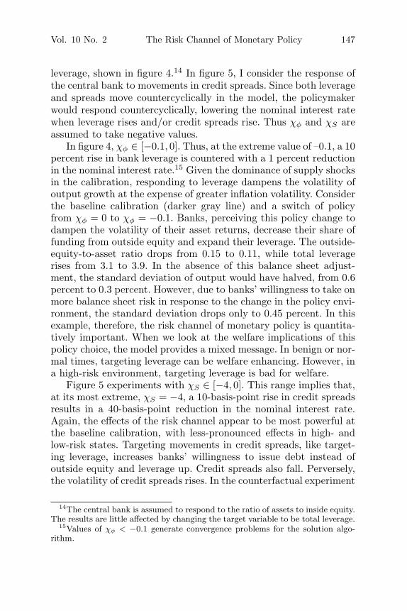
leverage, shown in figure 4.14 In figure 5, I consider the response ofthe central bank to movements in credit spreads. Since both leverageand spreads move countercyclically in the model, the policymakerwould respond countercyclically, lowering the nominal interest ratewhen leverage rises and/or credit spreads rise. Thus χφ and χS areassumed to take negative values.

In figure 4, χφ ∈ [−0.1, 0]. Thus, at the extreme value of –0.1, a 10percent rise in bank leverage is countered with a 1 percent reductionin the nominal interest rate.15 Given the dominance of supply shocksin the calibration, responding to leverage dampens the volatility ofoutput growth at the expense of greater inflation volatility. Considerthe baseline calibration (darker gray line) and a switch of policyfrom χφ = 0 to χφ = −0.1. Banks, perceiving this policy change todampen the volatility of their asset returns, decrease their share offunding from outside equity and expand their leverage. The outside-equity-to-asset ratio drops from 0.15 to 0.11, while total leveragerises from 3.1 to 3.9. In the absence of this balance sheet adjust-ment, the standard deviation of output would have halved, from 0.6percent to 0.3 percent. However, due to banks’ willingness to take onmore balance sheet risk in response to the change in the policy envi-ronment, the standard deviation drops only to 0.45 percent. In thisexample, therefore, the risk channel of monetary policy is quantita-tively important. When we look at the welfare implications of thispolicy choice, the model provides a mixed message. In benign or nor-mal times, targeting leverage can be welfare enhancing. However, ina high-risk environment, targeting leverage is bad for welfare.

Figure 5 experiments with χS ∈ [−4, 0]. This range implies that,at its most extreme, χS = −4, a 10-basis-point rise in credit spreadsresults in a 40-basis-point reduction in the nominal interest rate.Again, the effects of the risk channel appear to be most powerful atthe baseline calibration, with less-pronounced effects in high- andlow-risk states. Targeting movements in credit spreads, like target-ing leverage, increases banks’ willingness to issue debt instead ofoutside equity and leverage up. Credit spreads also fall. Perversely,the volatility of credit spreads rises. In the counterfactual experiment

14The central bank is assumed to respond to the ratio of assets to inside equity.The results are little affected by changing the target variable to be total leverage.

15Values of χφ < −0.1 generate convergence problems for the solution algo-rithm.


Figure 4. Effect of Variation in Monetary Policy Responseto Leverage

0.1

0.2

Out

side

eq.

/ as

sets

(lhs

, squ

ares

)To

tal l

ever

age

(rhs

, lin

e)

Bank balance sheet

3

4

1

1.2

1.4


38

39

40

41

42Capital stock

0.20.40.60.8

11.21.4


% re

lativ

e to

det.

ss

5

10

15


−0.1 −0.05 0

0.4

0.5

0.6

0.7


χφ

−0.1 −0.05 00.6

0.8

1

1.2


χφ




Figure 5. Effect of Variation in Monetary Policy Responseto Credit Spread

0.1

0.2

Out

side

eq.

/ as

sets

(lhs

, squ

ares

)To

tal l

ever

age

(rhs

, lin

e)

Bank balance sheet

3

4

1

1.2

1.4


39.5

40

40.5

41

41.5

Capital stock

0.2

0.4

0.6

0.8

1

1.2


% re

lativ

e to

det.

ss

1

2

3

4

5


−4 −3 −2 −1 0

0.3

0.4

0.5

0.6

0.7


χS

−4 −3 −2 −1 0

0.6

0.8

1


χS




with no risk channel (the dotted line), a change in policy towardsresponding aggressively to movements in credit spreads would haveyielded a reduction in the standard deviation of the credit spreadfrom 0.9 percent to below 0.8 percent. However, with the risk chan-nel present, the increase in bank leverage results in the standarddeviation of credit spreads actually rising, to close to 1.1 percent. Incontrast to targeting leverage, however, the risk channel amplifiesthe standard deviation of inflation while dampening the standarddeviation of output growth, relative to the model solution withoutthe risk channel.

The results presented in this section suggest that the risk channelof monetary policy, has, under certain policy prescriptions, mean-ingfully sized economic effects. Policymakers should be aware ofthis endogenous risk channel via endogenous changes in bank bal-ance sheets, especially if they aim to redesign policy to target spe-cific financial-sector indicators using the standard tools of monetarypolicy.

5. Conclusion

There is a popular view that the Great Moderation of the 1990s andearly 2000s sowed the seeds of the global financial crisis in 2007. Asmacroeconomic outcomes became less uncertain, financial interme-diaries built up leverage and took on more risk. In turn, anotherliterature has tried to explain the causes of the Great Moderation,from which two main views have emerged. One is a good-luck story,that the global economy simply enjoyed a period in which the shockshitting the economy were unusually modest. The other view is thatcentral banks had a better design of monetary policy.

This paper explores the risk channel of monetary policy in aquantitative macroeconomic model by endogenizing the compositionof banks’ funding. I find that when central banks target financialvariables such as cyclical leverage or credit spreads, policy can alterbanks’ balance composition in a quantitatively meaningful way, andaffect how shocks are amplified and propagated through the finan-cial sector. The numerical experiments in this paper suggest thatcentral banks and financial-sector regulators should be vigilant ofhow periods of relative tranquility (like the Great Moderation) cangenerate a potential buildup of risks in the economy as financial


institutions increase the size and leverage of their balance sheetsand rely more heavily on debt financing.

One possible line of further investigation would be to considermacroprudential policy alongside standard monetary policy. I leavethis for future research. My current avenue of research is to solve foroptimal (monetary) policy in this model.

Appendix 1. Risk-Adjusted Steady-State and First-OrderDynamics: Theory

This section explains how to solve a model as a first-order approx-imation of the model around a second-order approximation of themodel’s risk-adjusted steady state.

Let the equilibrium conditions of the model be written as

Et [f (yt+1, yt, xt+1, xt, zt+1, zt)] = 0 (36)

zt+1 = ρzt + ησεt+1,

where yt is an ny × 1 vector of endogenous non-predetermined vari-ables, xt is an nx × 1 vector of endogenous predetermined variables,zt is an nz × 1 vector of exogenous variables, and εt is an nz × 1vector of exogenous i.i.d. innovations with mean zero and unit stan-dard deviations. The matrices ρ and η are of order nz × nz and σ isa scalar scaling the amount of uncertainty in the economy.

Next, let the (unknown) decision rules that solve the systemof equations in (36) be yt = g(xt, zt) and xt+1 = h(xt, zt). Therisk-adjusted steady state, xr, solves

xr = h (xr, 0) with yr = g (xr, 0) . (37)

Substituting the decision rules into (36) and evaluating at the (alsoas yet unknown) risk-adjusted steady state gives

f (xr, σ) ≡ Et [f (g (xr, ησεt+1) , g (xr, 0) , xr, xr, ησεt+1, 0)] = 0.

Note that εt+1 is not an argument but, instead, the variable ofintegration inside the expectations operator. Taking a second-orderapproximation of f around σ = 0 (but a first-order approximationof g(.) and h(.)) gives

[f (xr, σ)]i ≈ [f (xr, 0)]i +σ2

2[fσσ (xr, 0)]i = 0, (38)


where

f (xr, 0) = f (yr, yr, xr, xr, 0, 0)

and

[fσσ (xr, 0)]i = [fy′y′ ]iαγ [gzη]αφ [gzη]γξ [I]φξ + [fy′z′ ]iαδ [gzη]αφ [η]δξ [I]φξ

+ [Θz′z′ ]iβδ [η]βφ [η]δξ [I]φξi = 1, . . . , n; α, γ = 1, . . . , ny; β, δ = 1, . . . , nz; φ, ξ = 1, . . . , nε.

The notation follows that in Schmitt-Grohe and Uribe (2004). Thefirst derivatives of the decision rules, gx, are solved using standardmethods of first-order approximation. The solution is found by iter-ating between a set of steady-state values (y, x) and a set of decisionrule coefficients (gz) until convergence is achieved.16

Appendix 2. Equilibrium Conditions

The model presented in section 2 has twenty-three endogenousvariables, {Ct, It, Kt, Nt, φt, QK,t, QE,t, RN,t, Rt, UC,t, Bt, Yt, Πt, Lt,Λt−1,t, Xt, μS,t, μE,t, μN,t, Ωt, RE,t, RK,t, St}, and twenty-three equi-librium equations, listed below.

Aggregate resource constraint:

(

1 − ϕΠ

2(Πt − 1)2

)

Yt = Ct +

(

1 +ϕI

2

(

It

It−1− 1

)2)

It.

Capital accumulation:

Kt+1 = (1 − δ) exp (εK,t) Kt + It.

Price of capital:

QK,t = 1 +ϕI

2

(

It

It−1− 1

)2

+(

It

It−1

)

ϕI

(

It

It−1− 1

)

− EtΛt,t+1

(

It+1

It

)2

ϕI

(

It+1

It− 1

)

.

16Code to implement this solution algorithm and replicate the results in thepaper is available from the author on request.


Inverse of banking sector’s inside-equity-to-asset ratio:

φt =QK,tKt+1

Nt.

Banking sector’s inside-equity accumulation:

Nt = θ ((RK,t − RE,tBt−1 − Rt (1 − Bt−1)) φt−1 + Rt) Nt

+ ωQK,tKt.

Household Euler equation and arbitrage condition:

EtΛt,t+1Rt+1 = 1 and EtΛt,t+1 (RE,t+1 − Rt+1) = 1.

Household stochastic discount factor:

Λt−1,t = βUC,t

UC,t−1.

Banking sector’s binding incentive compatibility constraint:

φt =μN,t

κ0(

1 + κ1Bt + κ22 B2

t

)

− (μS,t + BtμE,t).

Banking sector’s optimal leverage/outside equity trade-off:

μE,t

μS,t + BtμE,t=

κ1 + κ2Bt

1 + κ1Bt + κ22 B2

t

.

Return on capital and outside equity:

RK,t = exp (εK,t)Xtα

Yt

exp(εK,t)Kt+ (1 − δ) QK,t

QK,t−1

RE,t = exp (εK,t)Xtα

Yt

exp(εK,t)Kt+ (1 − δ) QE,t

QE,t−1.

Labor market equilibrium:

Xt (1 − α) YtUC,t = �L1+ϑt

(

Ct − hCt−1 − �

1 + ϑL1+ϑ

t

)−ζ

.


Marginal utility of consumption:

UC,t =(

Ct − hCt−1 − �

1 + ϑL1+ϑ

t

)−ζ

− ξtβh

(

Ct+1 − hCt − �

1 + ϑL1+ϑ

t+1

)−ζ

.

Aggregate production function:

Yt = exp(εA,t)(exp(εK,t)Kt)αL1−αt .

Banking sector’s marginal value of intermediating an additional unitof credit, of substituting one unit of debt for one unit of outsideequity, and of an additional unit of net worth, respectively:

μK,t = Et(Λt,t+1Ωt+1(RK,t+1 − Rt+1))

μE,t = Et(Λt,t+1Ωt+1(Rt+1 − RE,t+1))

μN,t = Et(Λt,t+1Ωt+1)Rt+1.

Shadow value of net worth:

Ωt = (1 − θ) + θBtφt.

Phillips curve:

ϕΠ

(

Πt

Π− 1

)

Πt

Π= 1 − ε (1 − Xt)

+ ϕΠEt

{

Λt,t+1

(

Πt+1

Π− 1

)

Πt+1

ΠYt+1

Yt

}

.

Monetary policy reaction function:(

RN,t

RN

)

=( (

Πt

Π

)χΠ(

Xt

X

)χX(

φt

φ

)χφ

× exp (χS (St − S))(

RK,t

RK

)χRK(

QK,t

QK

)χQK)1−χRN

×(

RN,t−1

RN

)χRN

exp (εM,t)


Credit spread:

St = EtRK,t+1 − Rt+1.

Fisher relation:

RN,t = Rt+1Et (Πt+1) .

Appendix 3. Steady State

We find a first-order approximation of the model in the neighbor-hood of the risk-adjusted steady state. With the exception of Bt,μE,t, and St—which remain in levels—all the variables are expressedas log-deviations. The steady-state inflation rate is set at Π = 1and Λ = β. This steady state is solved as described in appendix 2.The steady-state counterparts of the static equations simply involveremoving the time subscripts. The forward-looking equilibrium equa-tions are approximated to second order around σ = 0 (and the σis normalized to 1). The risk-adjusted steady-state correction terms(the second-order terms) are given by the M’s. At the deterministicsteady state, the M’s are zero. Equivalently, the deterministic steadystate is a zeroth-order approximation of the steady-state equationsaround σ = 0.

Price of capital:

QK = 1 + M1.

Household Euler equations:

1 = ΛR + M2 and 1 = Λ (RE − R) + M3.

Marginal utility of consumption:

UC = (1 − βh)(

(1 − h) C − �

1 + ϑL1+ϑ

)−ζ

+ M4.

Credit spread:

S = RK − R + M5.


Banking sector’s marginal value of intermediating an additional unitof credit, of substituting one unit of debt for one unit of outsideequity, and of an additional unit of net worth, respectively:

μS = ΛΩ (RK − R) + M6

μE = ΛΩ (R − RE) + M7

μN = ΛΩR + M8.

Phillips curve:

X =ε − (1 + M9)

ε.

Fisher relation:

RN = R + M10.

The risk-adjusted steady-state correction terms are as follows:

M1 ≡ −12ΛϕI

nε∑

i=1

(

5(

gIi

)2+ 2gΛ

i gIi

)

η2i

M2 ≡ 12ΛR

nε∑

i=1

(

gΛi

)2η2

i

M3 ≡ 12Λ

nε∑

i=1

(

(RE − R)(

gΛi

)2+ RE

(

2gΛi gRE

i +(

gREi

)2))

η2i

M4 ≡ 12ζβh

(

(1 − h) C − �

(1 + ϑ)L

(1+ϑ)t+1

)−ζ−1

×nε∑

i=1

⎛

⎜

⎜

⎜

⎜

⎜

⎜

⎜

⎜

⎜

⎝

C

(

1 − (1 + ζ)C(

(1 − h)C − �(1+ϑ)L

(1+ϑ))−1

)

(

gCi

)2

+ 2(1 + ζ)C�L1+ϑ(

(1 − h)C − �(1+ϑ)L

(1+ϑ))−1

gCi gL

i

− �L(1+ϑ)(

(1 + ϑ) + (1 + ζ) �L(1+ϑ)

×(

(1 − h) C − �(1+ϑ)L

(1+ϑ))−1

)

(

gLi

)2

⎞

⎟

⎟

⎟

⎟

⎟

⎟

⎟

⎟

⎟

⎠

η2i

M5 ≡ −12RK

nε∑

i=1

(

gRKi

)2η2

i


M6 ≡ 12ΛΩ (RK − R)

nε∑

i=1

(

(

gΛi

)2+ 2gΛ

i gΩi +

(

gΩi

)2)

η2i

M7 ≡ −12ΛΩ

(

(RE − R)(

(

gΛi

)2+ 2gΛ

i gΩi +

(

gΩi

)2)

(RE − R)

+ RE

(

2gΛi gRE

i + 2gΩi gRE

i +(

gREi

)2) )

M8 ≡ 12ΛΩR

nε∑

i=1

(

(

gΛi

)2+ 2gΛ

i gΩi +

(

gΩi

)2)

η2i

M9 ≡ 12ΠΛϕΠ

nε∑

i=1

(

3(

gΠi

)2+ 2gΛ

i gΠi + 2gΠ

i gYi

)

η2i

M10 ≡ 12ΠR

nε∑

i=1

(

gΠi

)2η2

i ,

where nε is the number of exogenous shocks and i = {A, K, M}indexes the shock. For example, gC

A is the first-order response ofconsumption (on impact) of a shock to technology.

Appendix 4. Welfare

Welfare at time t is denoted

Wt = Et

∞∑

i=0

βiU (Ct+i, Lt+i) .

In recursive form, welfare can be written as

Wt = U (Ct, Lt) + βEtWt+1.

At the risk-adjusted steady state, this becomes

W =U (C, L) +MW

1 − β,

where the risk adjustment takes the form

MW ≡ W2

(

gWi

)2η2

i .


Given initial policy A and alternative policy B, the consumption-equivalent compensation required to be indifferent about switchingfrom A to B is λu and is implicitly given by

WB =U

(

(1 − λu) CA, LA)

+MAW

1 − β.

Given the first-order approximation of the decision rule, Wt = g(xt)around the risk-adjusted steady state with policy B,

log Wt − log WB = gWx

(

log xt − log xB)

,

the welfare of policy B, conditional on initially being at the statevector xA (i.e., the risk-adjusted steady state with policy A), denotedWB|A, is

log WB|A − log WB = gWx

(

log xA − log xB)

.

To rewrite this level of welfare in terms of consumption-equivalentunits, λc, I calculate

WB|A =U

(

(1 − λc) CA, LA)

+MAW

1 − β.

References

Benigno, G., P. Benigno, and S. Nistico. 2013. “Second-OrderApproximation of Dynamic Models with Time-Varying Risk.”Journal of Economic Dynamics and Control 37 (7): 1231–47.

Bernanke, B., and M. Gertler. 1989. “Agency Costs, Net Worth,and Business Fluctuations.” American Economic Review 79 (1):14–31.

Bianchi, J. 2011. “Overborrowing and Systemic Externalities in theBusiness Cycle.” American Economic Review 101 (7): 3400–3426.

Calomiris, C. W., and C. M. Kahn. 1991. “The Role of DemandableDebt in Structuring Optimal Banking Arrangements.” AmericanEconomic Review 81 (3): 497–513.

Calvo, G. 1983. “Staggered Prices in a Utility-Maximizing Frame-work.” Journal of Monetary Economics 12 (3): 383–98.


Chari, V., and P. Kehoe. 2009. “Bailouts, Time Inconsistency andOptimal Regulation.” Unpublished Manuscript.

Coeurdacier, N., H. Rey, and P. Winant. 2011. “The Risky SteadyState.” American Economic Review 101 (3): 398–401.

Collard, F., and M. Juillard. 2001. “Accuracy of Stochastic Pertur-bation Methods: The Case of Asset Pricing Models.” Journal ofEconomic Dynamics and Control 25 (7): 979–99.

de Groot, O. 2012. “Coordination Failure and the Financial Accel-erator.” Unpublished Manuscript.

———. 2013. “Computing the Risky Steady State of DSGE Mod-els.” Economics Letters 120 (3): 566–69.

Devereux, M. B., and A. Sutherland. 2011. “Country Portfolios inOpen Economy Macro-Models.” Journal of the European Eco-nomic Association 9 (2): 337–69.

Diamond, D., and R. Rajan. 2009. “Illiquidity and Interest RatePolicy.” NBER Working Paper No. 15197.

Evans, M. D., and V. Hnatkovska. 2012. “A Method for SolvingGeneral Equilibrium Models with Incomplete Markets and ManyFinancial Assets.” Journal of Economic Dynamics and Control36 (12): 1909–30.

Farhi, E., and J. Tirole. 2012. “Collective Moral Hazard, MaturityMismatch, and Systemic Bailouts.” American Economic Review102 (1): 60–93.

Gertler, M., and P. Karadi. 2011. “A Model of Unconventional Mon-etary Policy.” Journal of Monetary Economics 58 (1): 17–34.

Gertler, M., and N. Kiyotaki. 2010. “Financial Intermediation andCredit Policy in Business Cycle Analysis.” In Handbook of Mon-etary Economics, Vol. 3, ed. B. M. Friedman and M. Woodford,547–99 (chapter 11). Elsevier.

Gertler, M., N. Kiyotaki, and A. Queralto. 2012. “Financial Crises,Bank Risk Exposure and Government Financial Policy.” Journalof Monetary Economics 59 (S0): S17–34.

Goldstein, I., and A. Pauzner. 2005. “Demand-Deposit Contractsand the Probability of Bank Runs.” Journal of Finance 60 (3):1293–1327.

Hart, O., and J. Moore. 1994. “A Theory of Debt Based on theInalienability of Human Capital.” Quarterly Journal of Econom-ics 109 (4): 841–79.


Keen, B., and Y. Wang. 2007. “What Is a Realistic Value for PriceAdjustment Costs in New Keynesian Models?” Applied Econom-ics Letters 14 (11): 789–93.

Kiyotaki, N., and J. Moore. 1997. “Credit Cycles.” Journal of Polit-ical Economy 105 (2): 211–48.

Kliem, M., and A. Meyer-Gohde. 2013. “Monetary Policy and theTerm Structure of Interest Rates.” Unpublished Manuscript.

Korinek, A. 2011. “Systemic Risk-Taking: Amplification Effects,Externalities, and Regulatory Responses.” ECB Working PaperNo. 1345.

Lorenzoni, G. 2008. “Inefficient Credit Booms.” Review of EconomicStudies 75 (3): 809–33.

Modigliani, F., and M. Miller. 1958. “The Cost of Capital, Corpo-ration Finance and the Theory of Investment.” American Eco-nomic Review 48 (3): 261–97.

Nikolov, K. 2010. “Is Private Leverage Excessive?” UnpublishedManuscript.

Rotemberg, J. 1982. “Monopolistic Price Adjustment and AggregateOutput.” Review of Economic Studies 49 (4): 517–31.

Schmitt-Grohe, S., and M. Uribe. 2004. “Solving Dynamic GeneralEquilibrium Models Using a Second-Order Approximation to thePolicy Function.” Journal of Economic Dynamics and Control 28(4): 755–75.

Smets, F., and R. Wouters. 2007. “Shocks and Frictions in US Busi-ness Cycles: A Bayesian DSGE Approach.” American EconomicReview 97 (3): 586–606.

Stein, J. 2012. “Monetary Policy as Financial Stability Regulation.”Quarterly Journal of Economics 127 (1): 57–95.

Townsend, R. 1979. “Optimal Contracts and Competitive Marketswith Costly State Verification.” Journal of Economic Theory 21(2): 265–93.

Date post:	02-Jul-2018
Category:	Documents
Upload:	truonghanh
View:	217 times
Download:	0 times

The Risk Channel of Monetary Policy - IJCB · The Risk Channel of Monetary Policy ... ness of the...

Documents