1 The Risk of a Currency Swap: A Multivariate-Binomial Methodology T.S. Ho Richard C. Stapleton * Department of Accounting and Finance The Management School, Lancaster University Lancaster LA1 4YX, UK. Tel:(+44) 1524-593-637 Fax:(+44) 1524-847-321 e-mail: [email protected]Marti G. Subrahmanyam ** Leonard N. Stern School of Business, New York University Management Education Center 44 West 4th Street, Suite 9--190 New York, NY10012--1126, USA. Tel: (+1) 212-998-0348 Fax: (+1) 212-995-4233. * We thank the participants at the annual meeting of the European Financial Management Association, in Innsbruck, Austria, in June 1966 and, in particular, the discussant of the paper, Bernard Dumas for helpful comments. Thanks are also due to Daniel J. Stapleton for able research assistance. We acknowledge the use of the programs, RMAUDIT and RMCORRISK supplied by RMAS Ltd. ** Please send proofs to Marti G. Subrahmanyam.
Transcript
1
The Risk of a Currency Swap:A Multivariate-Binomial Methodology
T.S. HoRichard C. Stapleton*
Department of Accounting and FinanceThe Management School, Lancaster University
Leonard N. Stern School of Business, New York UniversityManagement Education Center44 West 4th Street, Suite 9--190
New York, NY10012--1126, USA.Tel: (+1) 212-998-0348Fax: (+1) 212-995-4233.
* We thank the participants at the annual meeting of the European Financial Management Association,
in Innsbruck, Austria, in June 1966 and, in particular, the discussant of the paper, Bernard Dumas forhelpful comments. Thanks are also due to Daniel J. Stapleton for able research assistance. Weacknowledge the use of the programs, RMAUDIT and RMCORRISK supplied by RMAS Ltd.
** Please send proofs to Marti G. Subrahmanyam.
2
Executive Summary
The concept of "value-at-risk" (VAR) - the maximum loss on a specified horizon date at agiven level of confidence - is widely used at various levels of the financial system. Individualtraders and trading desks use the concept to determine the range of their potential gains andlosses over the next trading day. The managers of financial institutions apply the notion ofVAR to measure and control the risks of traders. Regulatory authorities, concerned with thestability of the financial system and of the institutions under their jurisdiction, set capitaladequacy standards based on measures of VAR. No matter what the specific criteria fordisclosure and capital adequacy are, a financial intermediary needs to translate the regulatoryrequirements into a practical system for implementation. The system needs to take intoaccount market data such as interest rates and exchange rates, as well as the detailedcharacteristics of the portfolio of assets and liabilities held by the intermediary, in order tovalue the portfolio on future dates and measure its response to changes in the market prices.
Although the broad approach to the measurement of the risk has to be consistently appliedacross financial instruments, the precise implementation depends on the instrument in question,and in particular, on the variables that affect its value on the future date. In this paper, the caseof a widely-used contract, the currency swap, is examined in some detail, to illustrate ourapproach. The value of a currency swap on a future date depends on a number of variables:the interest rates in the two currencies and the foreign exchange rate. Hence, the probabilitydistribution of the value of the swap on this date can be computed using the valuation modelfor the instrument and the joint probability distribution of these rates.
In order to estimate the joint distribution of these variables, it is useful to start from a model ofthe term structure of interest rates. The simplest possible model for a currency swap wouldinvolve only three variables: one determining the term structure in each of the two currencies,and one representing the exchange rate between the currencies. For some swaps, this mightbe a reasonable specification and we retain this as a special case of our model. However, as inthe case of fixed income securities and derivatives even in a single currency, a two-factormodel in at least one of the currencies will usually be required, in order to capture both shiftsand tilts in the term structure. To be specific, we might assume that for each of the twocurrencies involved in the swap, two "factor" rates determine the whole term structure. Then,we need to take into account the correlation between these rates and the exchange ratebetween the two currencies. The future exchange rate is relevant since the valuation of theswap involves the conversion of the cash flows into the numeraire currency. Hence, we needto model the stochastic behavior of five variables.
We use a method developed in an earlier paper [Ho, Stapleton and Subrahmanyam (1995)] toobtain the joint distribution of the five variables. In particular, we compute a multivariate-binomial distribution that approximates a joint-lognormal distribution with given means,volatilities and correlations. Essentially, the method yields an approximation to the jointdistributions of the variables using a joint binomial distribution, with the approximation gettingbetter as the binomial density for each variable is increased. For example, with three binomial
stages, each variable has a four state distribution and there are then 45 = 1024 scenarios ofinterest rates and exchange rates. The output is the joint distribution of the variables i.e., theset of interest rate and exchange rate scenarios and their probabilities. These are then used tocompute values of the currency swaps. This methodology is applied in a single-period context,
3
producing a single five-dimensional vector of interest rates and currencies together with thejoint-probability of each scenario. These inputs are then used to value the currency swap ineach scenario and to produce a probability distribution for the value of the swap. The resultingprobability distribution of the swap value can either be used to highlight particular,problematic scenarios, or to compute portfolio values at various confidence levels. Thus, theproposed methodology can be used to obtain conventional measures of VAR or to performscenario-based stress tests.
The main advantage of the proposed methodology is that it provides a computationally fastand efficient scenario analysis, allowing a state-by-state valuation of the swap. Particular statescan be identified where the swap is significantly exposed to market movements, so that the riskmanager can take appropriate action. Since the binomial density can be chosen at a differentlevel for each factor, it can be useful for sensitivity analysis of the valuation, after the mostsignificant variables have been identified. If one of them is the exchange rate, for example, thesimulation can be re-run with a greater density for the exchange rate. The other advantage isthat relatively few parameters are required in order to implement the model.
In the case of currency swaps, the valuation involves discounting the future cash flow streamsin the two currencies. Although this is fairly straight-forward conceptually, there is a practicalproblem in dealing with a large number of cash flows arising on different future dates. Acommon way of reducing the number of dates to be considered in measuring the market riskof a large swap portfolio is to use a "bucketing" methodology. Essentially, this is a way ofreducing the number of maturity dates of the future cash flows and is based on interpolation ofthe term structure. Thus, a small number of discount factors for standard maturity dates issufficient to value a complex portfolio with cash flows on several hundred dates.
Apart from computation of VAR, the methodology proposed in the paper can be used forpractical problems of risk management such as stress testing and credit risk. Stress testingnormally refers to the testing of model assumptions and parameters under extreme conditions.Illustrative examples used in the paper are departures from the assumption of joint-lognormality and high values of the volatilities and correlations. Credit risk can be analysed byexamining the risk-time profile of the swap position i.e., the risk exposure on different dates inthe future. This may be useful for analyzing the credit risk of the swap book.
4
Abstract
In general, the risk of a financial instrument on a future valuation date depends on severalstochastic variables. In the case of a currency swap, its value on a future date, can bemodelled as a function of five stochastic variables. These represent the factors that determinethe term structure of interest rates in the two currencies, and the foreign exchange ratebetween the currencies. The joint-probability distribution of the the relevant variables on thehorizon date of is approximated by a multivariate-binomial distribution. The proposedmethodology provides a fast and flexible alternative to Monte-Carlo simulation of the swapvalue. The distributions of value produced by the method can be employed to assist with bothmarket and credit risk management.
5
The Risk of a Currency Swap:A Multivariate-Binomial Methodology
1. Introduction
There has been considerable interest in recent years in the measurement of the risk of financial contracts. Theconcept of “value-at-risk” (VAR) - the maximum loss on a specified horizon date at a given level ofconfidence- is widely used at various levels of the financial system.1 Individual traders and trading desks usethe concept to determine the range of their potential gains and losses over the next trading day. The managersof financial institutions apply the notion of VAR to measure and control the risks of traders. Regulatoryauthorities, concerned with the stability of the financial system and of the institutions under their jurisdiction,set capital adequacy standards based on measures of value-at-risk.
The regulatory concerns have manifested themselves in a global context in discussions under the auspices ofthe Bank of International Settlements (BIS). A typical comment in these deliberations is that “quantitativeinformation about risk exposures and risk management performance can provide a framework for qualitativedescription and assessment.”2 It is clear that, no matter what the specific criteria for disclosure and capitaladequacy are, a financial intermediary needs to translate these into a practical system for implementation. Thesystem needs to take market data such as interest rates and exchange rates, as well as the detailedcharacteristics of the portfolio of assets and liabilities held by the intermediary into account, in order to valuethe portfolio on future dates and measure its response to changes in the market prices.
Although the broad approach to the measurement of the risk has to be consistently applied across financialinstruments, the precise implementation depends on the instrument in question, and in particular, on thevariables that affect its value on the future date. In this paper, the case of a common contract, the currencyswap, is examined in some detail. The value of a currency swap on a future date depends on a number ofvariables. For example, the value of a five-year fixed-for-fixed USD-DEM (U.S. Dollar-Deutsche Mark) swapin one year’s time will depend upon the USD interest rates for up to four years maturity in one year’s time, theDM interest rates for similar maturities and the foreign exchange rate of DEM for USD. The probabilitydistribution of the value of the swap depends on the valuation model and the joint distribution of these rates.In order to estimate the joint probability distribution of these variables it is useful to start from a model of theterm structure of interest rates. To be specific, we might assume that for each of the two currencies involved inthe swap, two “factor” rates determine the whole term structure. Then, we need to estimate the relationship ofthese rates with the exchange rate between the two currencies. The future exchange rate is relevant since thevaluation of the swap involves the conversion of the cash flows into the numeraire currency. is required in oneof the two currencies of the swap. In this paper, we propose and illustrate a procedure for determining thevalue of such a swap, assuming that a simple two-factor model holds for the term structure of interest rates ineach of the two currencies.
The simplest possible model for a currency swap would involve only three variables : one determining the termstructure in each of the two currencies, and one representing the exchange rate between the currencies. Forsome swaps, this might be a reasonable specification and we retain this as a special case of our model.However, as in the case of fixed income securities and derivatives even in a single currency, a two-factor modelin at least one of the currencies will usually be required, in order to capture both shifts and tilts in the termstructure. This is because swaps often involve fixed cash flows over reasonably long periods of time such asfive years. The approach here, therefore, allows for the possibility of a two-factor model in each of thecurrencies. Along with the currency factor, this means that we need to model the stochastic evolution of fivevariables.
6
Most of the term-structure models in the literature analyse the period-by-period movements of interest rates upto some terminal valuation date. This is true, for example, of the models of Ho and Lee (1986), Black, Dermanand Toy (1990), Heath, Jarrow and Morton (1992), and Hull and White (1993). A five-dimensional version ofany of those models would be prohibitively expensive from a computational point of view, and perhapsinfeasible, given currently available computing power. Luckily, for the purpose of risk management such amodel is not strictly required. In the context of risk management, it is sufficient to value a swap on a particulardate in the future, termed the value date. Thus, it is usually only necessary to model the joint distribution of thefive variables on that date, rather than to model the evolution of the variables at a series of intermediate dates,up to the value date. This makes the problem far more manageable.
A method for computing a multivariate-binomial distribution that approximates a joint-lognormal distributionof a specified number of variables, with given means, volatilities and correlations is proposed in Ho, Stapletonand Subrahmanyam (1995) (HSS). The method was applied in a portfolio management context in Ho,Stapleton and Subrahmanyam (1995a) and the application is extended here to the case of five variables. Thedistribution generated by this method converges to a joint-lognormal distribution, with the specifiedparameters, as the density of the binomial tree increases. In the present paper, we apply this methodology in asingle-period context, producing a single five-dimensional vector of interest rates and currencies together withthe joint-probability of each scenario. These inputs are then used to value the currency swap in each scenarioand to produce a probability distribution for the value of the swap. The resulting probability distribution of theswap value can either be used to highlight particular, problematic scenarios or to compute portfolio values atvarious confidence levels. Thus, the proposed methodology can be used to obtain conventional measures ofVAR or to perform scenario-based stress tests.
The outline of the paper is as follows. Section 2 presents a definition of the cash flows of a currency swap andprovides a general valuation formula for the value of the swap in the numeraire currency given that a separatetwo-factor model of the term structure of interest rates holds for each currency. A practical approach to thevaluation of a large currency swap book via the “bucketing” of the swap cash flows is described in section 3.Section 4 explains how to employ the multivariate-binomial approximation technique to generate scenarios ofthe relevant interest rates and exchange rates. Section 5 shows how to implement the two-factor model to valuethe swap cash flows in terms of the numeraire currency. Section 6 illustrates the output of the analysis using anumerical example. Section 7 concludes.
2. The Cash Flows of Currency Swaps
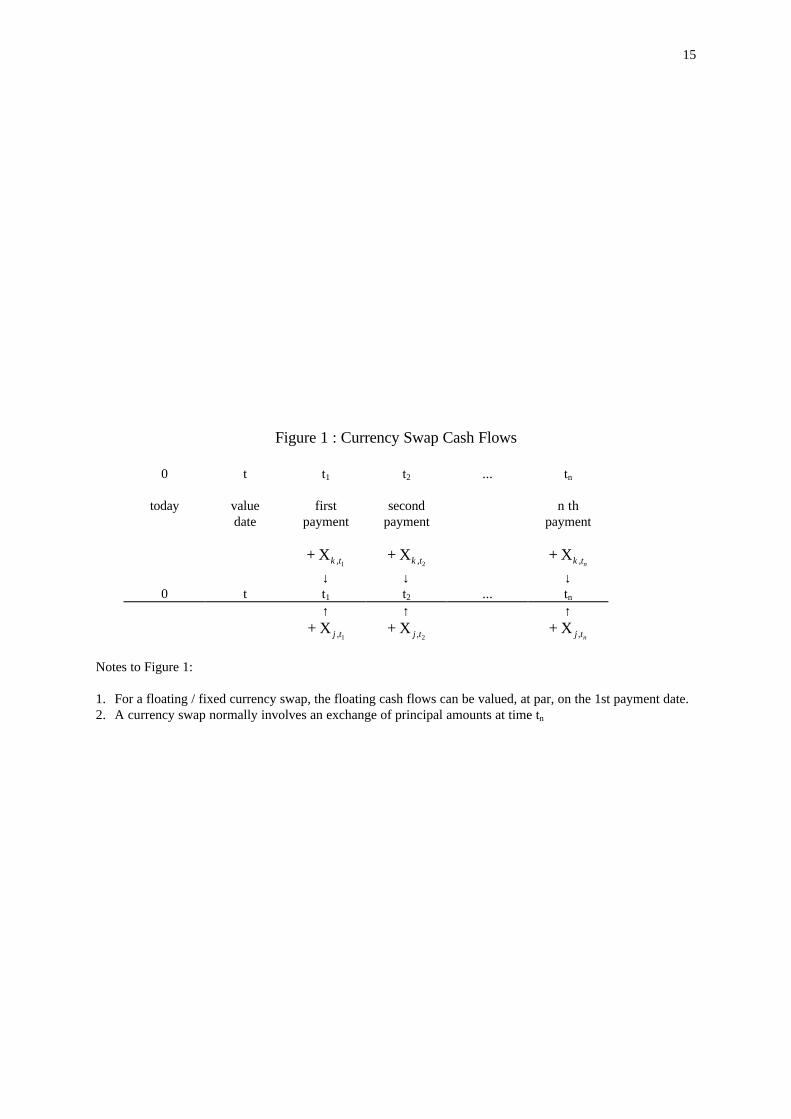
A currency swap involves cash flows in two currencies, which will be indexed by the subscripts j and k. In theFigure 1 below, we illustrate the flows for a swap where cash flows are paid in currency j and received incurrency k.
Figure 1 here
Figure 1 summarises the cash flows of a currency swap. The relevant dates are shown at the top of thediagram. We assume that a swap contract is in place at time 0 and is to be valued at time t. The payment datesfor the swap cash flows are t1, t2,...,ti,...,tn Hence, the currency swap involves the exchange of a stream of cashflows Xk t, 1
, Xk t, 2,…, Xk ti, ,..., Xk tn, in currency k for the stream X j t, 1
, X j t, 2,..., X j ti, ,…, X j tn, in
currency j. The cash flows shown on the time line are all non-stochastic. If the swap involves floatingpayments we assume that these are valued, at par, on the first reset date.
We assume that valuation is required in the numeraire currency j. The value of the swap at time t in currency jis
[ ][ ]
V X B X B X B P
X B X B X B
j t k t k t t k t k t t k t k t t j k t
j t j t t j t j t t j t j t t
n n
n n
, , , , , , , , , , , ,
, , , , , , , , ,
...
...
= + + +
− + + +
1 1 2 2
1 1 2 2
equation (1)
where
7
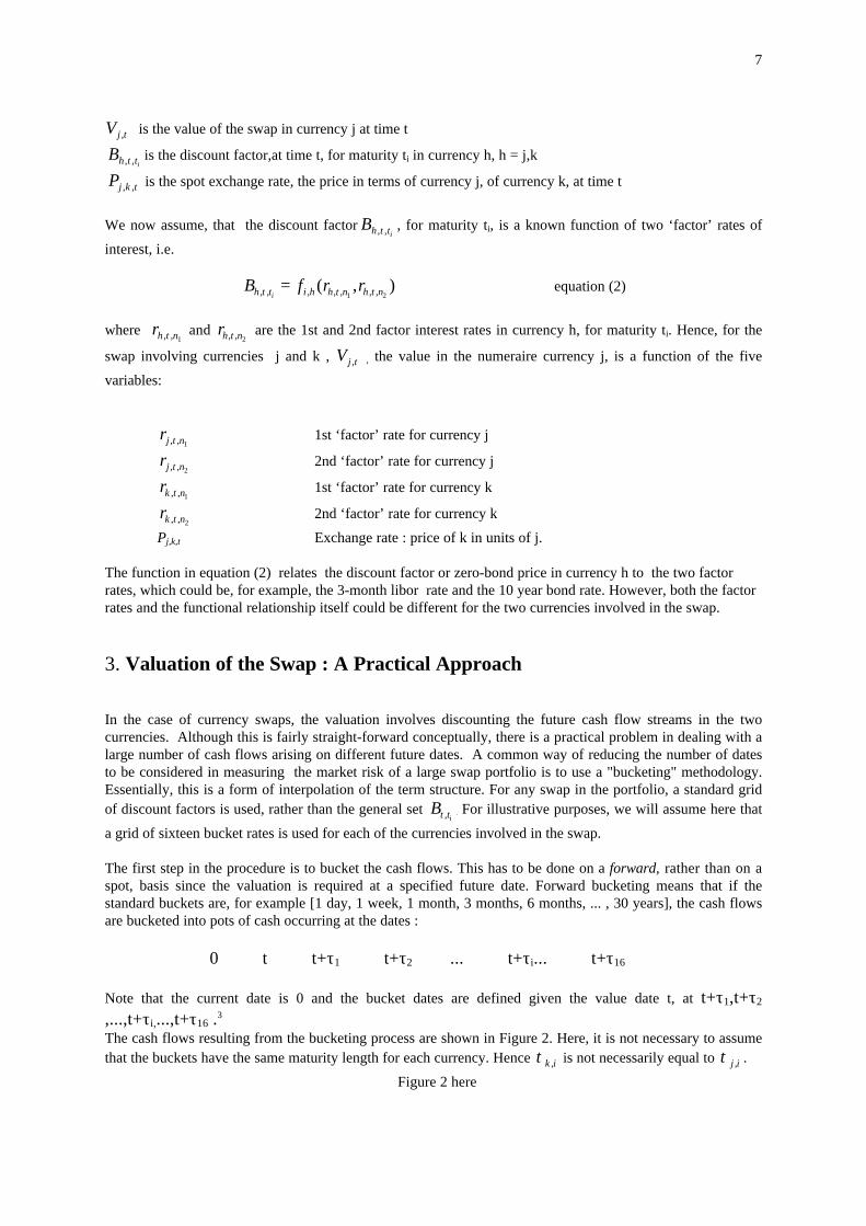
V j t, is the value of the swap in currency j at time t
Bh t ti, , is the discount factor,at time t, for maturity ti in currency h, h = j,k
Pj k t, , is the spot exchange rate, the price in terms of currency j, of currency k, at time t
We now assume, that the discount factor Bh t ti, , , for maturity ti, is a known function of two ‘factor’ rates of
interest, i.e.
B f r rh t t i h h t n h t ni, , , , , , ,( , )=1 2
equation (2)
where rh t n, , 1 and rh t n, , 2
are the 1st and 2nd factor interest rates in currency h, for maturity ti. Hence, for the
swap involving currencies j and k , V j t, , the value in the numeraire currency j, is a function of the five
variables:
rj t n, , 11st ‘factor’ rate for currency j
rj t n, , 22nd ‘factor’ rate for currency j
rk t n, , 11st ‘factor’ rate for currency k
rk t n, , 22nd ‘factor’ rate for currency k
Pj,k,t Exchange rate : price of k in units of j.
The function in equation (2) relates the discount factor or zero-bond price in currency h to the two factorrates, which could be, for example, the 3-month libor rate and the 10 year bond rate. However, both the factorrates and the functional relationship itself could be different for the two currencies involved in the swap.
3. Valuation of the Swap : A Practical Approach
In the case of currency swaps, the valuation involves discounting the future cash flow streams in the twocurrencies. Although this is fairly straight-forward conceptually, there is a practical problem in dealing with alarge number of cash flows arising on different future dates. A common way of reducing the number of datesto be considered in measuring the market risk of a large swap portfolio is to use a "bucketing" methodology.Essentially, this is a form of interpolation of the term structure. For any swap in the portfolio, a standard gridof discount factors is used, rather than the general set Bt ti, . For illustrative purposes, we will assume here that
a grid of sixteen bucket rates is used for each of the currencies involved in the swap.
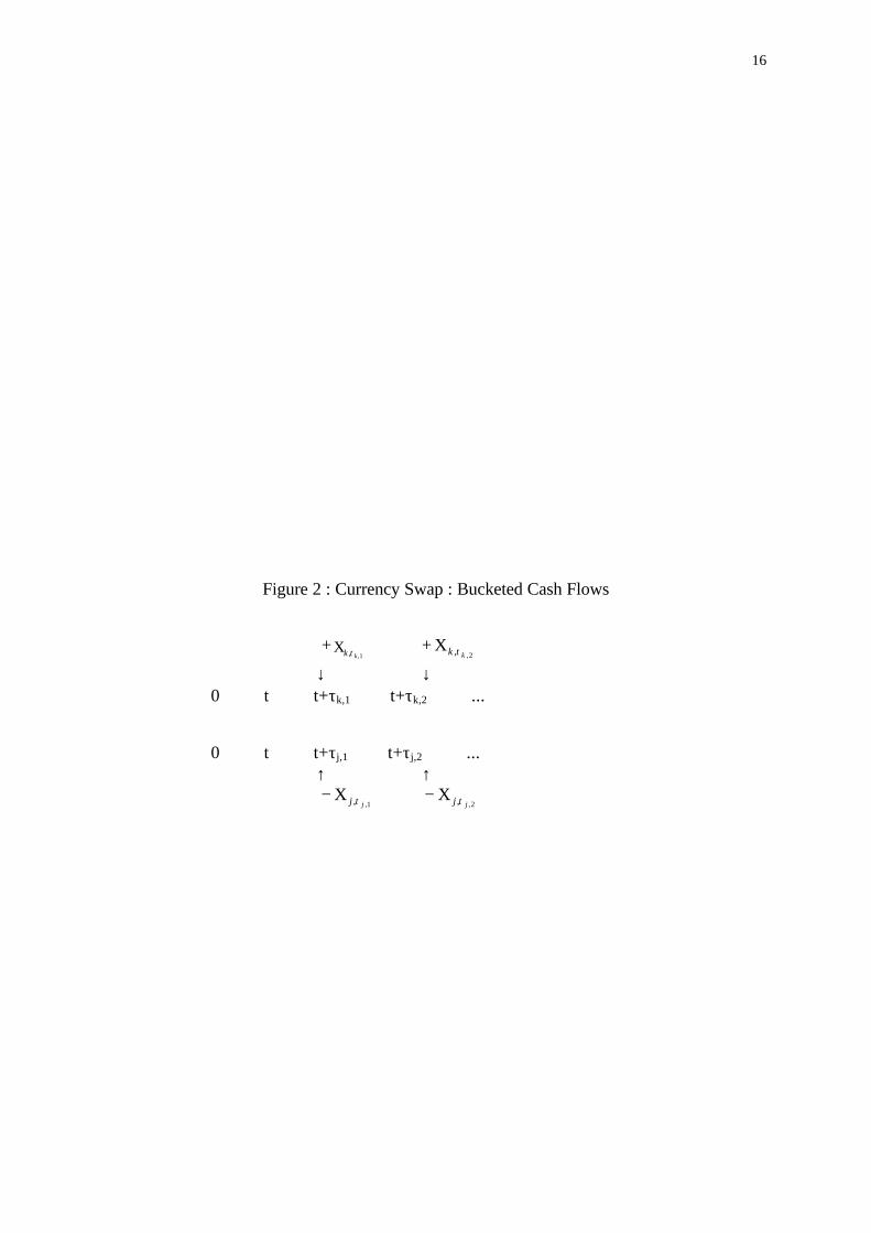
The first step in the procedure is to bucket the cash flows. This has to be done on a forward, rather than on aspot, basis since the valuation is required at a specified future date. Forward bucketing means that if thestandard buckets are, for example [1 day, 1 week, 1 month, 3 months, 6 months, ... , 30 years], the cash flowsare bucketed into pots of cash occurring at the dates :
0 t t+τ1 t+τ2 ... t+τi... t+τ16
Note that the current date is 0 and the bucket dates are defined given the value date t, at t+τ1,t+τ2
,...,t+τi,...,t+τ16 .3
The cash flows resulting from the bucketing process are shown in Figure 2. Here, it is not necessary to assumethat the buckets have the same maturity length for each currency. Hence τ k i, is not necessarily equal to τ j i, .
Figure 2 here
8
Having bucketed the cash flows, we now require the discount factors for the standard grids in the twocurrencies and the exchange rates. We next describe the generation of scenarios of interest rates in thefollowing section.
4. The Joint-Probability Distribution of Factor Interest Rates and theExchange Rate
In order to value the swap, we need to generate a joint-probability distribution of the five variables thatdetermine its value. The most popular method employed in practice is to assume that the variables arelognormal with given means, variances and covariances and to construct a multivariate lognormaldistribution.4 Here we use a binomial approximation approach where the distribution limits to the lognormal asthe density of the binomial tree increases. This method has the advantage of allowing a scenario analysis, ofextreme states, to be performed.5 This is advantageous if we wish to use the output for an analysis of the creditrisk of a book of currency swaps.
Given that we wish to analyse individual states by building a binomial tree, a number of approaches have beensuggested in the literature. Most of these are surveyed in the recent paper by Amin (1995). One approach,suggested by He (1990) and Boyle (1989), models N variables using a binomial distribution with just N+1nodes over each sub-interval. This method is efficient in the context of valuing options whose payoff dependson more than one variable. However, in the context of risk analysis, we require to distinguish all possiblestates. We therefore favour the methodology of Ho, Stapleton and Subrahmanyam (1995). They build anapproximation to the joint distributions of the variables using a joint binomial distribution which produces(J+1)N nodes, where J is the binomial density for each variable.6 There are two ways of building such adistribution. First, it is possible to orthogonalize the variables and build the joint distribution of a set oforthogonal vectors. This method is illustrated in Amin (1991). However, the HSS methodology builds vectorsof the individual variables with just J+1 nodes for each variable. It captures the covariance structure byadjusting the conditional probabilities. This feature of the HSS method makes it somewhat simpler to employin the context of risk management, where the distributions of the individual variables, as well as themultivariate distribution may be relevant. To summarise, there are a number of advantages of the HSSapproach in this context. The main ones are :
• It is an efficient method of generating scenarios of the relevant interest rates and exchange rates.• If greater accuracy is required, at the expense of more computation time, then the number of binomial
stages can be increased. This increases the fineness or density of the binomial tree. It can also be done on avariable-by-variable basis.
• It allows specific scenarios to be investigated. The swap value can be computed for particular, unusualcombinations of interest rates and exchange rates. Thus, it gives more qualitative information to the riskmanager than a simple mean-variance analysis, for example.
The HSS methodology assumes that the underlying variables, in this application, the factor interest rates andthe exchange rate are joint-lognormally distributed. As a first approximation, this is perhaps not a badassumption, since it is the assumption underlying most of the option pricing models used in practice. Later,when we perform a stress test, the effect of relaxing this assumption is investigated. The required inputs for thejoint-lognormal distribution are the means, volatilities and correlations of the variables. These are specified inTable 1 below
Table 1 here
The input data can be estimated in many different ways, depending on the information available. However, areasonable procedure may be as follows :
1. Estimate the means of the factor interest rates from the forward rates at time 0 (the current date) fordelivery at the value date t.7 Also, estimate the mean of the exchange rate from the forward rate, at time 0,for deliveries of the currency at time t.
9
2. Estimate the volatilities using either historical data on the factor interest rates or by backing out impliedvolatilities from option prices. Based on the results in the empirical literature, the implied volatilities maybe upward-biased estimates of the true volatility.
3. Estimate the correlation matrix from historical data.8
The HSS methodology requires the choice of J, the binomial density, J, determines how many factor interestrates, exchange rates and scenarios are generated. For example, with J=3, each variable has a four statedistribution. There are then 45 = 1024 scenarios of factor interest rates and exchange rates. The output is thejoint distribution of the variables. Note that J can be chosen at a different level for each factor, if required. Thiscan be useful for sensitivity analysis of the valuation, after the most significant variables have been identified.If one of them is the exchange rate, for example, the simulation can be re-run with a greater density for theexchange rate. The output at this stage of the simulation is the set of factor interest rates and exchange ratescenarios and their probabilities. These numbers can now be used to compute value of the currency swap ineach scenario.
The methodology fits the input mean vector and the variance-covariance matrix by changing the conditionalprobabilities of the binomial tree.9 Details of the implementation of the approach are provided in theAppendix.
5. Swap Valuation in Each Scenario
In order to value the swap cash flows, we first need to specify the functional relationship between the discountfactors and the generated factor interest rates for each currency, shown generally in equation (2). We then needto compute the swap value in each scenario using equation (1). The choice of the particular interest rate modelto be used depends upon how closely we wish to model interest rate movements. Given the complexity of theproblem situation, we choose here a rather simple linear model for the spot rates of interest. Suppose that n1 isthe maturity in years of the first factor interest rate and n2 is the maturity of the second factor rate, then, foreach currency, we assume that the yield rate for the kth bucket maturity is10
rn
n nr
n
n nrt
it n
it ni, , ,τ
τ τ=
−−
+
−−
2
2 1
1
2 11 2
equation (3)
We then compute the required discount factors from the relationship
Brt tt
i
i
i,,( )+ =
+ττ
τ
11
equation (4)
The two-factor model of the interest rates in equation (3) is a simple “shift-tilt” model. The term structureshifts, if both the factor interest rates move in the same direction, and tilts, if one of the rates increases whilethe other falls. Also, given equation (3), the rate for any intermediate maturity is just a weighted average of thetwo factor rates, where the weights depend on the distance of the maturity from each of the factor ratematurities.
Given the discount factors for the bucket maturities, we can now value the bucketed cash flows using thevaluation equation :
[ ][ ]
V X B X B X B P
X B X B X B
j t k k t k k t k k t j k t
j j t j j t j j t
k k k k n k n k
j j j j n j n j
, , , , , , , , , , , ,
, , , , , , , , ,
, , , , , ,
, , , , , ,
...
...
= + + +
− + + +
τ τ τ τ τ τ
τ τ τ τ τ τ
1 1 2 2
1 1 2 2
equation (5)
10
Here, the general valuation equation (1) has been adjusted so that all the cash flows occur only on the bucketdays. This revised valuation equation can now be used to compute the swap value in each scenario of theinterest rate and exchange rate.
6. Scenario Analysis of the Value of a Currency Swap : An Illustration
Equation (5) above can be evaluated in each scenario, given its probability of occurrence, to yield a probabilitydistribution of the value of the swap. We can obtain an estimate of the VAR by ranking the states by the valueof the swap and reading off the value at any given confidence level. Of more relevance, however, is the state bystate analysis of possible values of the swap position. This is given by the joint-probability distributionproduced by the binomial model.
As an illustration, we take a JPY/ DEM currency swap with the cash flows shown in Table 2.
Table 2 here
The swap is a three year “receive floating-DEM, pay fixed-JPY” swap with a principal of 50,000,000DM. Thecurrent date 11/5/95. The exchange rate is 65Yen per DM on the current date, 11/5/95. The term structures forthe two currencies on 11/5/95 are as follows.
Table 3 here
Note that the yields in Table 3 are yields on zero-coupon bonds for the given maturities. Here, we haveassumed, for simplicity, that the bucket maturities are the same for each currency. The yield curves for bothcurrencies are generally upward sloping with the Yen yields somewhat lower than those for the DM.
The problem is to calculate value of the swap cash flows estimates on a value date 90 days hence. The first stepis to bucket the swap cash flows into standard buckets. It yields the cash flows shown in Table 4.
Table 4 here
The first swap payment date is 11/09/96, which is four months from the current date, or one month from thevaluation date. Hence, the first cash flow is allocated to the one-month bucket. The later cash flows for thefixed Yen payments are bucketed in the 6 month, 1 year, 2 year and 3 year buckets.
We now proceed to generate scenarios for the interest rate term structures and exchange rate on the valuationdate. The input data for the simulation is shown in Table 5.
Table 5 here
The HSS model assumes that the variables are joint-lognormally distributed with given means, volatilities andcorrelations. The means for the short and long rates and the exchange rates are taken to be the respectiveforward rates. In turn, these are computed from the zero-coupon bond yields and the given spot exchange rate.Reasonable estimates for the volatilities and correlations have been assumed.
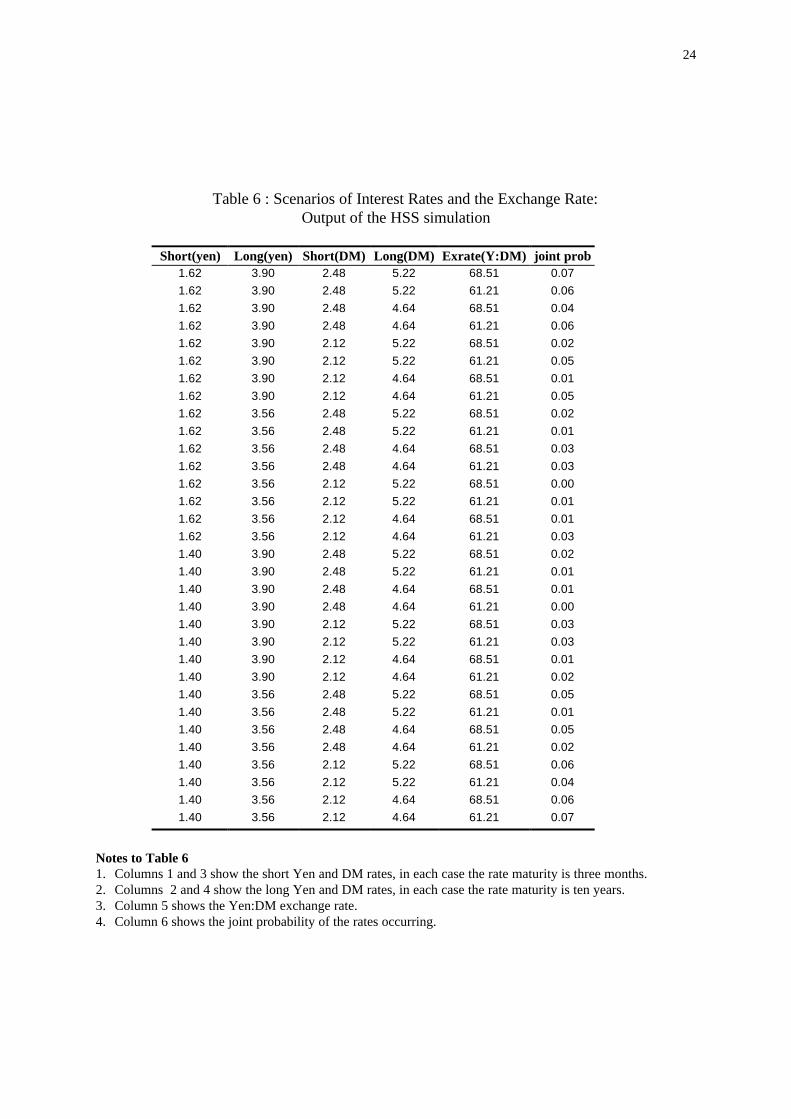
We run the HSS model with, for illustrative purposes, J=1 for each variable. This produces 25 = 32 scenarios.These are shown in Table 6. The probability of each scenario is shown in the last column of Table 6.
Table 6 here
Note that the methodology captures the correlation structure by building a binomial distribution for the firstvariable (yen short rate factor) with two nodes, for the second variable (yen long rate factor) with four nodes,
11
and so on up to thirty-two nodes for the fifth variable (the exchange rate). Also, the joint probabilities arechosen so as to approximate the means, variances and correlations of the variables. The methodology is testedand shown to converge, as N increases, to the given parameter value. For each scenario, we now model theterm structure for the two currencies using equation (3). The resulting rates are shown in Table 7.
Table 7 here
In Table 7, we show only the rates from six months to five years for each currency. (Note that all sixteenbucket rates are actually computed for each currency, although only some of them are relevant for thisexample.) In the cross-sectional model for the term structure using equation (3), the computed rates are simpleweighted- averages of the two factor rates, where the weights reflect the distance of the bucket maturity fromthe two factor rates.
We now use the term structure scenarios to value the two sets of bucketed cash flows, using equations (4) and(5). The results are shown in the following Table 8.
Table 8 here
Columns six and eight of Table 8 show the cumulative probability distribution of the swap value in Yen. Thisis computed by valuing the Yen and DM cash flows, in each scenario, and then converting the DM value intoYen at the exchange rate prevailing in the scenario. The low values of the swap (from 133-155 million Yen)correspond to low Yen:DM exchange rates. The higher values are for the higher exchange rate. This showsthat the major risk, in this case, is the exchange rate volatility. The table can also be used to compute the swapvalue at a variety of confidence levels. For example, there is at least a 99% chance of the swap being of greatervalue than 134,678,753 Yen.
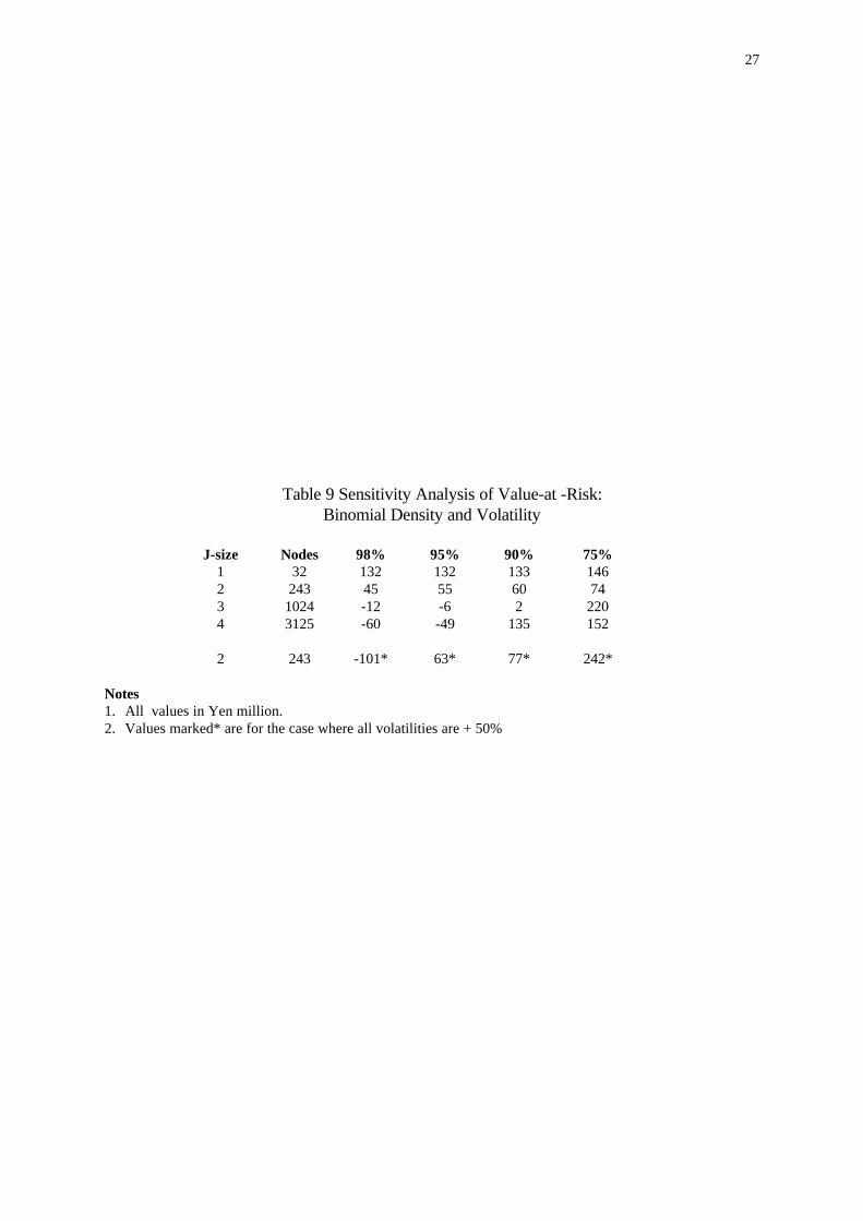
Table 9 here
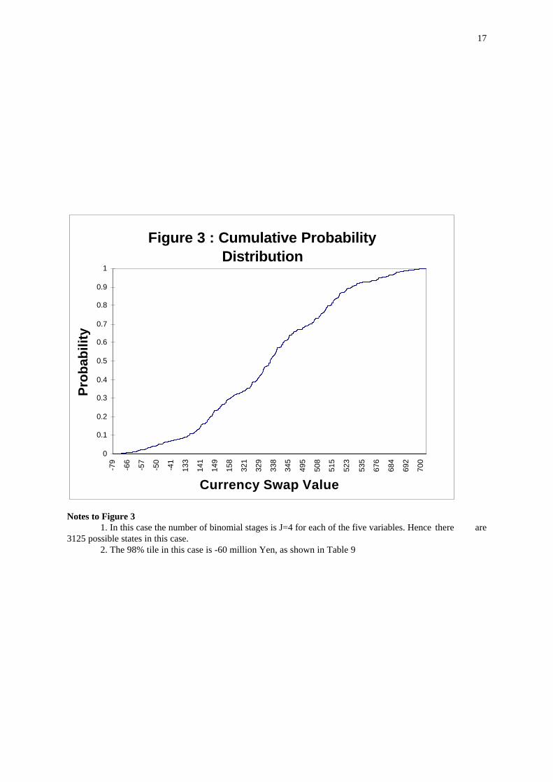
In Table 9, we show the effect of increasing the number of binomial stages. The confidence level values arequite sensitive to the binomial-density chosen. In Figure 3, we show the cumulative density in the case where J= 4. In the case of this currency swap, it is clear from Table 8 that the swap value is most sensitive to theexchange rate variable. An increase in the binomial density, J, has the effect of including a wider range ofpossible exchange rates. This effect can be seen in Figure 3, where the range has been considerably extendedcompared with the range for J = 1 shown in Table 9. This also has a radical effect on the percentile VARestimate.
Figure 3 here
Stress Testing of the Swap Value-at-Risk model
Stress testing normally refers to the testing of model assumptions and parameters. How sensitive are the resultsto the assumption that the interest rate factors and the exchange rate are joint-lognormally distributed, forexample? There is considerable empirical evidence that exchange rates, for example, are fat tailed compared tothe lognormal distribution. Also, a related fact is that the volatilities of both interest rates and exchange ratesare stochastic and correlated to the rates themselves. In table 9 we show the effect on the VAR estimates of re-running the simulation, for the case of J=2, assuming all volatilities are increased by 50%. Suppose that weexpect volatility to be high at the same time that an observation in the 5% tail of the distribution occurs. Theappropriate VAR at the 95% confidence level is that shown for the high volatility distribution.
Conclusions
This paper has illustrated how the HSS methodology, for approximating joint distributions of variables withbinomial distributions, can be applied in the case of a currency swap. The swap has first to be reduced to a set
12
of non-stochastic cash flows, in the two currencies. The inputs and outputs of the system are summarised in thediagram in Figure 4 below. The main inputs are the current term structures of the two currencies and theexchange rate, their respective volatilities, and the non-stochastic swap cash flows.
Figure 4 here
The procedure is then as follows :
1. Compute forward rates using the term-structure inputs, and exchange rates.2. Generate scenarios for the variables and probabilities using the HSS method. Use a two-factor model to
generate the term structure of zero-bond yields for each scenario.3. Given the future valuation date, bucket the swap cash flows into maturity buckets. Do this for each
currency.4. Value the bucketed cash flows in each currency using the relevant term structure.5. Convert the values into a common currency value and form the cumulative density of the swap value
The approach suggested for the risk evaluation of the currency swap, or book of currency swaps has thefollowing advantages :
a) It provides a computationally fast and efficient scenario analysis, allowing a state-by-state valuation of theswap. Particular states can be identified where the swap is particularly exposed to market movements.
b) Since the time to the value date can be varied, the method allows the analyst to build a risk-time profile ofthe swap position. This may be useful for analysing the credit risk of the swap book. The use of themethodology in the context of credit risk analysis is pursued in Stapleton and Subrahmanyam (1997)
c) Relatively few parameters need to be estimated in order to implement the model. Also the estimation anduse of statistically significant and stable parameters is possible.
13
References
Amin, K.I.(1991) “ On the Computation of Continuous Time Option Prices Using Discrete Approximations,”Journal of Financial and Quantitative Analysis, 26, 4, December, 477-495.
Bank of International Settlements, Discussion paper, September, 1995.
Black, F., E. Derman, and W. Toy (1990), “A One-Factor Model of Interest Rates and its Application toTreasury Bond Options,” Financial Analysts’ Journal, 33-339.
Boyle, P. “A Lattice Framework for Options Pricing when there are Two State Variables,” Journal ofFinancial and Quantitative Analysis, 23,1, March, 1-12.
He, H. (1990) , “Convergence from Discrete to Continuous-time Contingent Claims Prices,” Review ofFinancial Studies, 3, 523-546.
Heath, D., R.A. Jarrow, and A. Morton (1992), “Bond Pricing and the Term Structure of Interest Rate: A NewMethodology for Contingent Claims Valuation,” Econometrica, 60, 1, January, 77-105.
Ho, T.S.Y. and S.B. Lee (1986), “Term Structure Movements and Pricing of Interest Rate Claims,” Journal ofFinance, 41, December, 1011-1029.
Ho, T.S., R.C. Stapleton and M.G. Subrahmanyam, (1995) “Multivariate binomial approximations for assetprices with non-stationary variance and covariance characteristics.” Review of Financial Studies, 8, 1125-1152.
Ho, T.S., R.C. Stapleton and M.G. Subrahmanyam, (1995a) “Correlation Risk, Cross-market DerivativeProducts and Portfolio Performance Benchmarks.” European Financial Management, 1, 2, June, 105-124.
Ho, T.S., R.C. Stapleton and M.G. Subrahmanyam, (1996) “A Two-factor No-arbitrage model of the TermStructure of Interest Rates” Working paper, presented at Osaka International Conference on Finance, January1996,
Hull, J. and A. White (1993), “One-Factor Interest Rate Model and the Valuation of Interest Rate DerivativeSecurities,” Journal of Financial and Quantitative Analysis, June, 235-254,
Stapleton, R.C. and M.G. Subrahmanyam, (1997) , “Evaluating the Credit Risk of a Swap Portfolio: A Two-factor Model Approach,”, working paper.
14
Appendix
Methodology used for the multivariate-binomial approximation
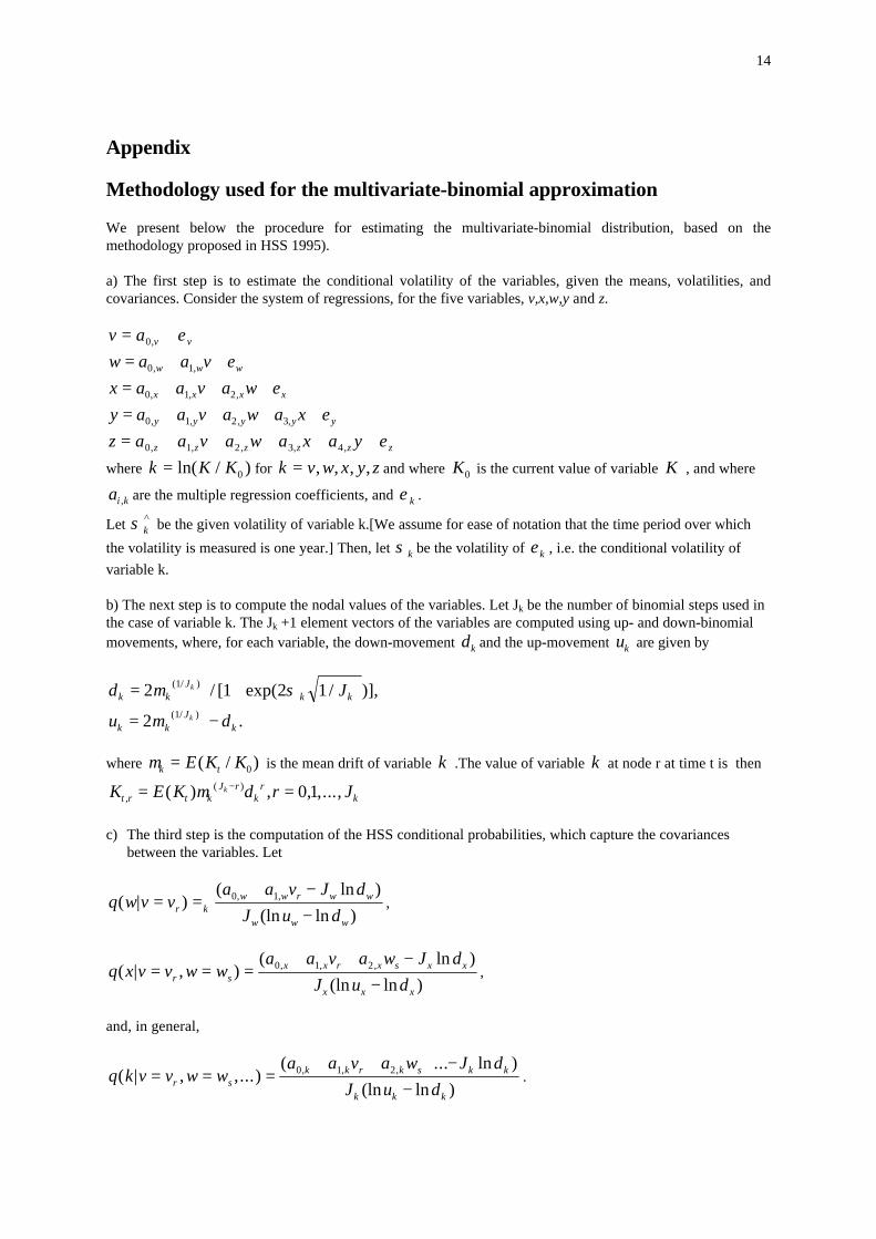
We present below the procedure for estimating the multivariate-binomial distribution, based on themethodology proposed in HSS 1995).
a) The first step is to estimate the conditional volatility of the variables, given the means, volatilities, andcovariances. Consider the system of regressions, for the five variables, v,x,w,y and z.
v a v v= +0, εw a a vw w w= + +0 1, , εx a a v a wx x x x= + + +0 1 2, , , εy a a v a w a xy y y y y= + + + +0 1 2 3, , , , εz a a v a w a x a yz z z z z z= + + + + +0 1 2 3 4, , , , , εwhere k K K= ln( / )0 for k v w x y z= , , , , and where K0 is the current value of variable K , and where
ai k, are the multiple regression coefficients, and ε k .
Let σ k^ be the given volatility of variable k.[We assume for ease of notation that the time period over which
the volatility is measured is one year.] Then, let σ k be the volatility of ε k , i.e. the conditional volatility of
variable k.
b) The next step is to compute the nodal values of the variables. Let Jk be the number of binomial steps used inthe case of variable k. The Jk +1 element vectors of the variables are computed using up- and down-binomialmovements, where, for each variable, the down-movement dk and the up-movement uk are given by
d Jk kJ
k kk= +2 1 2 11µ σ( / ) / [ exp( / )],
u dk kJ
kk= −2 1µ ( / ) .
where µk tE K K= ( / )0 is the mean drift of variable k .The value of variable k at node r at time t is then
K E K d r Jt r t kJ r
kr
kk
,( )( ) , , ,...,= =−µ 0 1
c) The third step is the computation of the HSS conditional probabilities, which capture the covariancesbetween the variables. Let
q w v va a v J d
J u dr kw w r w w
w w w
( | )( ln )
(ln ln ), ,= =
+ −−
0 1 ,
q x v v w wa a v a w J d
J u dr sx x r x s x x
x x x
( | , )( ln )
(ln ln ), , ,= = =
+ + −−
0 1 2 ,
and, in general,
q k v v w wa a v a w J d
J u dr sk k r k s k k
k k k
( | , ,...)( ... ln )
(ln ln ), , ,= = =
+ + + −−
0 1 2 .
15
Figure 1 : Currency Swap Cash Flows
0 t t1 t2 ... tn
today value first second n thdate payment payment payment
+ Xk t, 1+ Xk t, 2
+ Xk tn,
↓ ↓ ↓0 t t1 t2 ... tn
↑ ↑ ↑+ X j t, 1
+ X j t, 2+ X j tn,
Notes to Figure 1:
1. For a floating / fixed currency swap, the floating cash flows can be valued, at par, on the 1st payment date.2. A currency swap normally involves an exchange of principal amounts at time tn
16
Figure 2 : Currency Swap : Bucketed Cash Flows
+Xk k, ,τ 1+ Xk k, ,τ 2
↓ ↓0 t t+τk,1 t+τk,2 ...
0 t t+τj,1 t+τj,2 ...↑ ↑
− X j j, ,τ 1− X j j, ,τ 2
17
Figure 3 : Cumulative Probability Distribution
0
0.1
0.2
0.3
0.4
0.5
0.6
0.7
0.8
0.9
1
-79
-66
-57
-50
-41
133
141
149
158
321
329
338
345
495
508
515
523
535
676
684
692
700
Currency Swap Value
Pro
bab
ility
Notes to Figure 31. In this case the number of binomial stages is J=4 for each of the five variables. Hence there are
3125 possible states in this case.2. The 98% tile in this case is -60 million Yen, as shown in Table 9
18
Figure 4
VAR for Currency Swap : Flow Diagram
Term Structure YenTerm Structure DM
Ex rate Yen:DM
Probabilitydistribution
VAR, 99% level,state by state
Volatilities : 5Correlation matrix 5x5
Bucketingprocedure
StochasticTerm
structures,Ex rate
Swapvaluation,currency
conversion
Forward rates
Swap cash flows+Yen-DM
Notes to Figure 41. The flow chart shows the inputs, computations and the output of the currency swap risk model.
19
Table 1 : Inputs for HSS Simulation
Variable Mean Volatility Correlation Matrix1 2 3 4 5
Notes to Table 21. Columns 1 and 3 show the exact dates on which payments will be made. These are at six-monthly intervals.2. Column 2 shows the amounts in 000’s, adjusted for the exact day-count convention, that will be paid in
Yen.3. Column 4 shows the amounts in 000’s, adjusted for the exact day-count convention, that will be received in
Deutsche Marks. These floating payments have been valued on the first reset date of the swap.
21
Table 3 : Zero-Coupon Bond Yields
Term Structures on the analysis datematurity Yen yield curve DM yield curve
Notes to Table 41. Columns 1 and 3 show the maturity of the buckets in weeks (W), months (M) and years (Y). The first rate
maturity is the overnight (O/N) rate.2. Columns 2 and 4 show the Yen and DM cash flows respectively in 000’s.
23
Table 5 : Input data for Scenario Analysis
HSS model: Input Data
Short (yen) Long (yen) Short (DM) Long (DM) Exrate (Y:DM)
Means 1.51% 3.73% 2.30% 4.79% 64.86
Volatilities 0.14 0.10 0.16 0.12 0.12
Correlation matrix
Short (yen) 1 0.4 0.3 0 -0.2
Long (yen) 0.4 1 0.1 0.2 -0.1
Short (DM) 0.3 0.1 1 0 0.2
Long (DM) 0 0.2 0 1 0.1
Exrate (Y:DM) -0.2 -0.1 0.2 0.1 1
Notes to Table 5.1. The short and long rates are the 3 month and 10 year zero coupon bond rates in each case.2. The means are computed as the forward rates for 90 days forward. The mean exchange rate is the forward
exchange rate, assuming a current exchange rate of 65 Yen per DM.
24
Table 6 : Scenarios of Interest Rates and the Exchange Rate:Output of the HSS simulation
Notes to Table 61. Columns 1 and 3 show the short Yen and DM rates, in each case the rate maturity is three months.2. Columns 2 and 4 show the long Yen and DM rates, in each case the rate maturity is ten years.3. Column 5 shows the Yen:DM exchange rate.4. Column 6 shows the joint probability of the rates occurring.
25
Table 7 : Yen and DM Term Structures
Yen rates DM rates0.5 yr 1yr 2 yr 3 yr 4 yr 5 yr 0.5 yr 1yr 2 yr 3 yr 4 yr 5 yr1.67 1.79 2.03 2.26 2.50 2.73 2.55 2.69 2.97 3.25 3.53 3.81
Notes to Table 71. Columns 1-6 show the Yen rates, only rates for maturities of a half year to five years are shown.2. Columns 7-12 show the DM rates, again only rates for maturities of a half year to five years are shown.
26
Table 8 : Present Value Distribution of the Swap
PV Yen PV DM DM in Yen swap value joint prob swap value joint prob cum prob
1. Column 1 shows the Present value of the Yen fixed cash flows in each scenario.2. Column 2 shows the present value of the DM floating cash flows in DM.3. Column 3 shows the Yen value of the DM flows.4. Column 4 shows the value of the swap in each scenario.5. Column 5 shows the joint probability of the events, i.e. the probability of the scenario.6. Column 6 shows the ranking of the swap value by size, and column 7 shows the associated probability.
7. Column 8 shows the cumulative probability of the swap values.
27
Table 9 Sensitivity Analysis of Value-at -Risk:Binomial Density and Volatility
Notes1. All values in Yen million.2. Values marked* are for the case where all volatilities are + 50%
28
Footnotes
1 For example, the Working Group of the Euro-currency Standing Committee of the central banks of theGroup of Ten countries provides the following definition: “Value-at-Risk is a concept derived from statisticalestimates of the losses or gains a portfolio could experience, due to changes in underlying prices, over a givenholding period, for given confidence intervals.” (BIS Discussion Paper, September 1995)
2 See BIS Discussion Paper, September 1995.
3 The bucketing procedure is designed to maintain the present value of the cash flows and the sensitivity oftheirvalue to changes in interest rates.
4 The effect of relaxing the assumption of lognormality is analysed in the stress testing that is described insection 6 below.
5 An alternative, popular methodology is Monte Carlo simulation. However this is computationally expensive.
6 More accurately, the number of nodes is (J1 +1)(J2+1)…(JN+1) where Ji is the binomial density chosen forvariable i. An alternative approach is Monte Carlo simulation, which tends however to be computationallyexpensive. Also a full covariance matrix approach is possible. However this does not typically yieldinformation on a state-by-state basis.
7 If these are not directly available they can be computed from the spot rates for the two currencies.
8 As it is for example in the JP Morgan Riskmetrics system.
9 It is shown in HSS (1995) that the means, variances and covariances converges in the limit to the true valuesas the binomial density increases.
10 This model is a simplification of the no-arbitrage model of the term structure developed in HSS (1996)where the curvature of the term structure results partially from mean-reversion in the short rate factor. In themodel used in (3), simplicity is preferred to the more sophisticated mean reversing model in HSS (1996), sincethe issue here is not valuation, as such, but risk management.