The risk of harmful algal blooms (HABs) in the oyster-growing estuaries of New South Wales, Australia Penelope Ajani & Steve Brett & Martin Krogh & Peter Scanes & Grant Webster & Leanne Armand Received: 2 May 2012 / Accepted: 8 October 2012 / Published online: 31 October 2012 # Springer Science+Business Media Dordrecht 2012 Abstract The spatial and temporal variability of po- tentially harmful phytoplankton was examined in the oyster-growing estuaries of New South Wales. Forty- five taxa from 31 estuaries were identified from 2005 to 2009. Harmful species richness was latitudinally graded for rivers, with increasing number of taxa southward. There were significant differences (within an estuary) in harmful species abundance and richness for 11 of 21 estuaries tested. Where differences were observed, these were predominately due to species belonging to the Pseudo-nitzschia delicatissima group, Dinophysis acuminata, Dictyocha octonaria and Prorocentrum cordatum with a consistent upstream versus downstream pattern emerging. Temporal (seasonal or interannual) patterns in harmful phytoplankton within and among estuaries were high- ly variable. Examination of harmful phytoplankton in relation to recognised estuary disturbance measures revealed species abundance correlated to estuary mod- ification levels and flushing time, with modified, slow flushing estuaries having higher abundance. Harmful species richness correlated with bioregion, estuary modification levels and estuary class, with southern, unmodified lakes demonstrating greater species densi- ty. Predicting how these risk taxa and risk zones may change with further estuary disturbance and projected climate warming will require more focused, smaller scale studies aimed at a deeper understanding of species-specific ecology and bloom mechanisms. Coupled with this consideration, there is an imperative for further taxonomic, ecological and toxicological investigations into poorly understood taxa (e.g. Pseudo-nitzschia). Keywords Harmful algae . Estuary condition . Nutrients . Pseudo-nitzschia Introduction Marine phytoplanktons are arguably the most beauti- ful and important organisms on earth, being a funda- mental link in the global biogeochemical cycle and a critical component of marine food webs (Falkowski et Environ Monit Assess (2013) 185:5295–5316 DOI 10.1007/s10661-012-2946-9 P. Ajani (*) : L. Armand Department of Biological Sciences, Climate Futures at Macquarie, Macquarie University, North Ryde, NSW 2109, Australia e-mail: [email protected]S. Brett Microalgal Services, 308 Tucker Road, Ormond, VIC 3204, Australia M. Krogh : P. Scanes Waters and Coastal Science Section, New South Wales Office of Environment and Heritage, PO Box A290, Sydney South, NSW 1232, Australia G. Webster New South Wales Food Authority, 1 Macquarie Street, Taree, NSW 2430, Australia
Transcript
The risk of harmful algal blooms (HABs) in the oyster-growingestuaries of New South Wales, Australia
Penelope Ajani & Steve Brett & Martin Krogh &
Peter Scanes & Grant Webster & Leanne Armand
Received: 2 May 2012 /Accepted: 8 October 2012 /Published online: 31 October 2012# Springer Science+Business Media Dordrecht 2012
Abstract The spatial and temporal variability of po-tentially harmful phytoplankton was examined in theoyster-growing estuaries of New South Wales. Forty-five taxa from 31 estuaries were identified from 2005to 2009. Harmful species richness was latitudinallygraded for rivers, with increasing number of taxasouthward. There were significant differences (withinan estuary) in harmful species abundance and richnessfor 11 of 21 estuaries tested. Where differences wereobserved, these were predominately due to speciesbelonging to the Pseudo-nitzschia delicatissimagroup, Dinophysis acuminata, Dictyocha octonariaand Prorocentrum cordatum with a consistent
upstream versus downstream pattern emerging.Temporal (seasonal or interannual) patterns in harmfulphytoplankton within and among estuaries were high-ly variable. Examination of harmful phytoplankton inrelation to recognised estuary disturbance measuresrevealed species abundance correlated to estuary mod-ification levels and flushing time, with modified, slowflushing estuaries having higher abundance. Harmfulspecies richness correlated with bioregion, estuarymodification levels and estuary class, with southern,unmodified lakes demonstrating greater species densi-ty. Predicting how these risk taxa and risk zones maychange with further estuary disturbance and projectedclimate warming will require more focused, smallerscale studies aimed at a deeper understanding ofspecies-specific ecology and bloom mechanisms.Coupled with this consideration, there is an imperativefor further taxonomic, ecological and toxicologicalinvestigations into poorly understood taxa (e.g.Pseudo-nitzschia).
Keywords Harmful algae . Estuary condition .
Nutrients . Pseudo-nitzschia
Introduction
Marine phytoplanktons are arguably the most beauti-ful and important organisms on earth, being a funda-mental link in the global biogeochemical cycle and acritical component of marine food webs (Falkowski et
Environ Monit Assess (2013) 185:5295–5316DOI 10.1007/s10661-012-2946-9
P. Ajani (*) : L. ArmandDepartment of Biological Sciences,Climate Futures at Macquarie, Macquarie University,North Ryde, NSW 2109, Australiae-mail: [email protected]
S. BrettMicroalgal Services,308 Tucker Road,Ormond, VIC 3204, Australia
M. Krogh : P. ScanesWaters and Coastal Science Section, New South WalesOffice of Environment and Heritage,PO Box A290, Sydney South, NSW 1232, Australia
G. WebsterNew South Wales Food Authority,1 Macquarie Street,Taree, NSW 2430, Australia
al. 1998). Some species, however, can form harmfulalgal blooms (HABs). The causative organisms ofHABs include those that produce toxins that accumu-late in marine organisms (bivalves, fish, etc.) and maybe transferred to higher trophic levels affecting fish,mammals, birds and humans. Major toxic syndromescaused by these harmful algae are Paralytic ShellfishPoisoning (PSP), Diarrhetic Shellfish Poisoning (DSP),Neurotoxic Shellfish Poisoning and Amnesic ShellfishPoisoning (ASP). Other harmful algae do not producetoxins, but may cause fish kills due to oxygen depletionor gill damage (Hallegraeff et al. 2003; Pitcher 2012).
HAB events are considered to be increasing in fre-quency and occurrence worldwide (Hallegraeff 1993;van Dolah 2000; Anderson et al. 2008), and for thisreason, many countries throughout the world now con-duct HAB monitoring programs with the aim of mini-mising the economic and health effects related to theseepisodes. Design of monitoring programs varies consid-erably, reflecting differing goals, physical and biologicalregimes, available technology and administration. Onecommon key evaluation indicator of these programs hasbeen the development of a forecast capability that pro-vides both spatial and temporal information regardingrisk taxa and risk zones (UNESCO 1996). Studies in-vestigating the causative species and occurrence of toxicblooms (Rhodes et al. 2009; Hernandez-Becerril et al.2007; Verhsinin and Orlova 2008; Jester 2009), toxinproduction and shellfish toxicity (Thomas et al. 2010),human health perspectives (Moore et al. 2008), and thetemporal and spatial distribution of toxic phytoplanktonand toxic events throughout the world (Puigserver et al.2010; Phlips et al. 2010) are carried out to validatelocation-specific information. These studies provide anunderstanding of the patterns, interactions and scales ofphytoplankton variability (Cloern and Jassby 2010).Location-specific information also provides valuablefeedback for regulatory authorities allowing improve-ments to monitoring program design and decision mak-ing (Trainer et al. 2012).
The New South Wales Food Authority regulatesthe shellfish industry in New South Wales (NSW)in accordance with national and state legislation,which includes the NSW Shellfish Program andthe NSW Biotoxin Management Plan 2011(NSWBMP, http://www.foodauthority.nsw.gov.au/industry/industry-sector-requirements/shellfish/).The NSWBMP aims to ensure the protection ofshellfish consumers from the hazards of marine
biotoxin poisoning by regular monitoring of phy-toplankton and shellfish toxins. An early warningof the potential for contamination of shellfish leadsto real-time closures of harvest areas and providesan effective and co-ordinated response to harmfulevents. Similar biotoxin monitoring programs areundertaken in other Australian states, particularlyTasmania and South Australia.
New South Wales Estuaries
There are approximately 184 important estuaries alongapproximately 2,000 km of NSW coastline (Roper et al.2011), although Roy et al. (2001) noted that there couldbe as many as 950 water bodies joining the sea, the vastmajority of these water bodies being very small. Roy etal. (2001) described two primary processes that shapeestuaries: tidal domination (forming bays, basins anddrowned river valleys) and wave domination (formingbarrier rivers, lakes and lagoons), with the latter makingup at least 90 % of NSW estuaries. Within the wave-dominated estuary group, there are those associated withlarger rivers and whose estuary mouths occur behindsand barriers (barrier rivers); those associated with lowrelief, coastal plain coasts (lakes); and lagoons, usuallynon-tidal for long periods of time and which are rare inNSW (Roy et al. 2001). Within each estuary type, thereare different tidal exchange rates, flushing characteristics,capacities to trap or bypass contaminants and biotacomposition.
Compared to northern hemisphere estuaries,Australian estuaries are relatively poorly studied, but,with increasing coastal development and a focus onwater quality and future climate variability, the em-phasis on understanding these diverse systems is in-creasing (NLWRA 2001; Davis and Koop 2006).Scanes et al. (2007) evaluated the appropriateness ofwater quality-based indicators in NSW estuariesand reported that an increase in catchment distur-bance in coastal lagoons correlated poorly withmost of the commonly measured water qualityvariables. Whilst these authors found a significantrelationship between chlorophyll a and catchmentdisturbance, there has been no measure of therelationship between HAB species (many of whichare heterotrophic) and environmental variables inNSW estuaries.
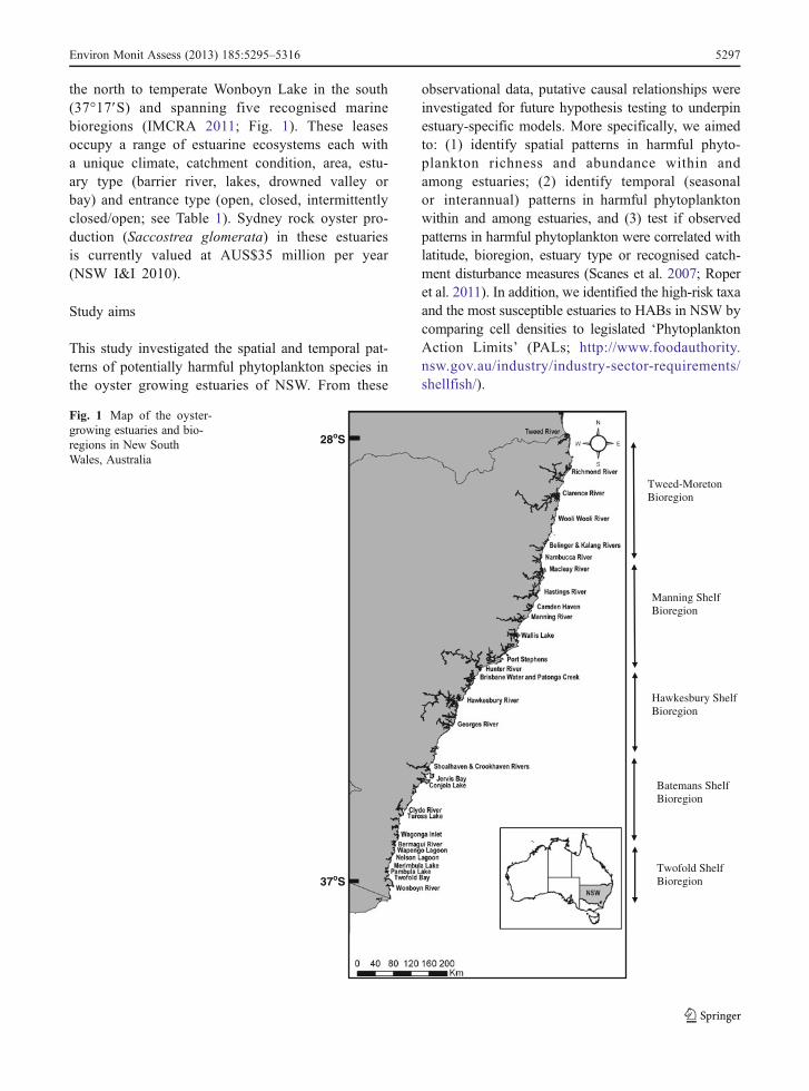
NSW oyster leases are found along the entire NSWcoast, from the sub-tropical Tweed River (28°10′S) in
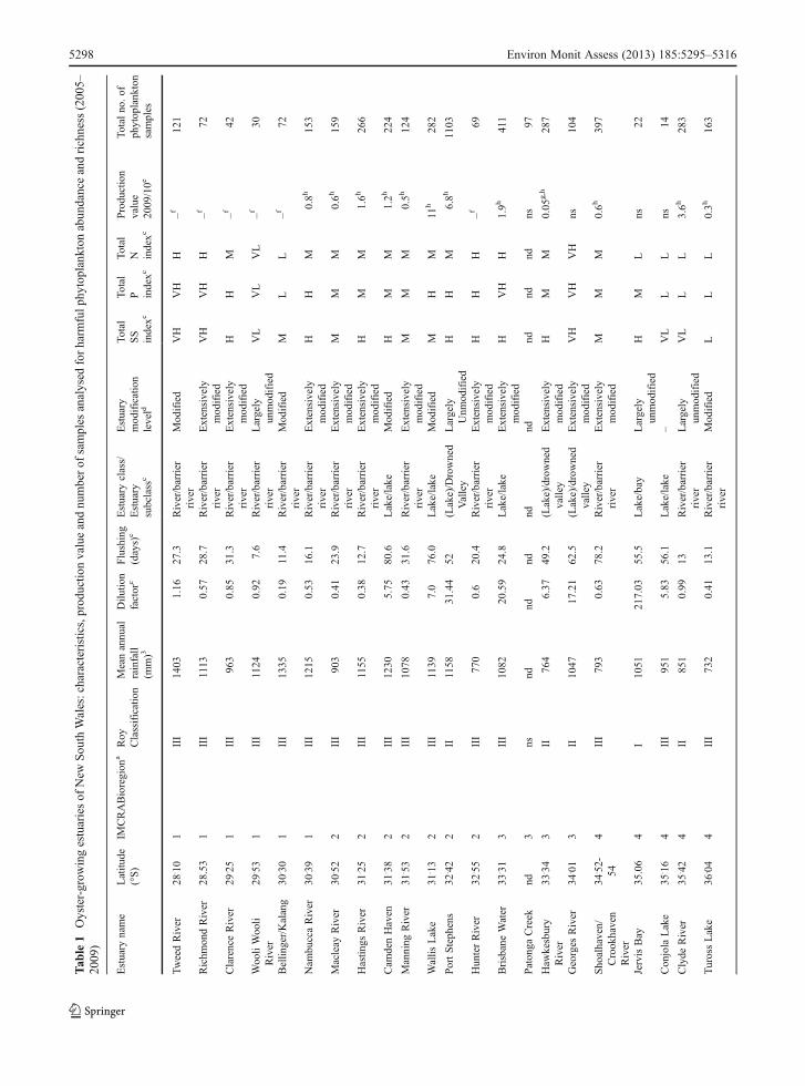
the north to temperate Wonboyn Lake in the south(37°17′S) and spanning five recognised marinebioregions (IMCRA 2011; Fig. 1). These leasesoccupy a range of estuarine ecosystems each witha unique climate, catchment condition, area, estu-ary type (barrier river, lakes, drowned valley orbay) and entrance type (open, closed, intermittentlyclosed/open; see Table 1). Sydney rock oyster pro-duction (Saccostrea glomerata) in these estuariesis currently valued at AUS$35 million per year(NSW I&I 2010).
Study aims
This study investigated the spatial and temporal pat-terns of potentially harmful phytoplankton species inthe oyster growing estuaries of NSW. From these
observational data, putative causal relationships wereinvestigated for future hypothesis testing to underpinestuary-specific models. More specifically, we aimedto: (1) identify spatial patterns in harmful phyto-plankton richness and abundance within andamong estuaries; (2) identify temporal (seasonalor interannual) patterns in harmful phytoplanktonwithin and among estuaries, and (3) test if observedpatterns in harmful phytoplankton were correlated withlatitude, bioregion, estuary type or recognised catch-ment disturbance measures (Scanes et al. 2007; Roperet al. 2011). In addition, we identified the high-risk taxaand the most susceptible estuaries to HABs in NSW bycomparing cell densities to legislated ‘PhytoplanktonAction Limits’ (PALs; http://www.foodauthority.nsw.gov.au/industry/industry-sector-requirements/shellfish/).
28oS
37oS
Tweed-Moreton Bioregion
Manning Shelf Bioregion
Hawkesbury Shelf Bioregion
Batemans Shelf Bioregion
Twofold Shelf Bioregion
Fig. 1 Map of the oyster-growing estuaries and bio-regions in New SouthWales, Australia
Fortnightly water samples (500 mL to 1 L) from adepth of 50 cm were collected from a total of 76harvest areas within 31 oyster growing estuaries for aperiod of 5 years (28 June 2005 to 7 December 2009)(Fig. 1). Lugol’s iodine was immediately added towater samples to preserve phytoplankton cells for lateridentification. In the laboratory, samples were concen-trated by gravity-assisted membrane filtration, and cellcounts were undertaken in a Sedgewick Rafter count-ing chamber. Highly toxic species, e.g. Alexandriumand Dinophysis were counted to a minimum detectionthreshold of 50 cells–L while all other species werecounted to a minimum detection threshold of500 cells–L. Cell counts and detailed examination ofcells were carried out using Zeiss Axiolab orZeiss Standard microscopes equipped with phasecontrast. Cells were identified to the closest taxonthat could be accurately identified using lightmicroscopy (maximum magnification ×1,000).Where accurate separation of species was not possibleusing light microscopy cells were assigned to a speciesgroup (e.g. Pseudo-nitzschia delicatissima group,Pseudo-nitzschia pungens/multiseries, etc). When nec-essary, detailed examination of dinoflagellate thecalplates (Fritz and Triemer 1985) stained withCalcofluor White were undertaken using ZeissStandard or Leitz Diavert microscopes equipped withUVepifluorescence.
The phytoplankton taxa deemed potentiallyharmful in the context of this study were a com-bination of:
1. Those taxa listed in the International Oceanographic–UNESCO Taxonomic Reference List of HarmfulMicroalgae (http://www.marinespecies.org/hab/);
2. Other local species belonging to the genera in thisreference list and
3. Other taxa that are known to cause indiscriminatefish kills due to oxygen depletion or gill damage(Hallegraeff et al. 2003)
In statistical analyses, seasons were defined asS0Summer (December–February), A0Autumn(March–May), W0Winter (June–August) andSP0Spring (September–November). A priorigroups of harvest areas, determined by the NSWBiotoxin Monitoring Program, were defined assites.
Phytoplankton community spatial and temporalpatterns
Large scale. A one-way ANOVA was used to deter-mine if the mean number of potentially harmful taxadiffered between the two primary estuary types (riverand drowned river valley + lake).
Small scale. Statistical analyses of small-scalespatial and temporal phytoplankton patterns wereundertaken using the multivariate statistical soft-ware PRIMER-E v6 (Clarke and Gorley 2006).Non-parametric analyses were used on: (1) abun-dance data (after a square-root transformation to‘down weight’ the most abundant toxic phyto-plankton taxa) and (2) taxa richness data (using apresence/absence transformation of abundance data;see Clarke and Warwick 2001). Taxa richness wasdefined as the number of potentially harmful phy-toplankton taxa in any given sample. Non-harmfultaxa were not enumerated in the current study andtherefore the more commonly used diversity indi-ces such as Shannon’s or Simpson’s indices werenot considered relevant descriptors for these data(Hill 1973).
Comparisons among estuaries were done usingmean abundance phytoplankton data that were ana-lysed using cluster analysis to examine any groupingsof estuaries (sites, years and seasons pooled).Comparisons within estuaries considered the influenceof two factors, sites and season. Sites were distributedwithin estuaries in three main patterns: ten estuarieshad only a single site, so no comparisons within estu-ary were possible; ten estuaries had sites that werespatially differentiated, with some sites in a “down-stream zone” less than 6 km from the entrance andother sites in an “upstream zone”more than 6 km fromthe entrance (“dispersed sites”) and 11 estuaries had“aggregated sites”—in this case, all the sites were in a“downstream zone.”
Differences among sites in estuaries with dispersedand aggregated sites were examined using multidi-mensional scaling to provide an ordination of the datausing the Bray–Curtis similarity measure (Clarke andWarwick 2001). Analysis of similarity (ANOSIM)was used to investigate differences among factors,and (where significant) the similarity percentagesprocedure (SIMPER), was used to identify the mostimportant phytoplankton taxa contributing to thesegroup discriminations (Clarke and Warwick 2001).
Statistical hypothesis tests used a type 1 error rate of5 % (i.e. α00.05), where ANOSIM tests identified astatistically significant global difference among treat-ment levels; pairwise tests were also conducted usinga type 1 error rate of 5 % (Clarke and Warwick 2001).Such pairwise comparisons were considered moresuitable as hypothesis generators as opposed to hy-pothesis proofs and adjustment of the type 1 error ratefor the number of factor levels (e.g. Bonferroni cor-rections) were not undertaken.
A subset of estuaries was selected for graphicalrepresentation to further illustrate the monthly andannual abundance patterns. The estuaries selectedwere those estuaries with high (or historically high)production values (Table 1)—Hastings River, CamdenHaven River, Wallis Lake, Port Stephens, HawkesburyRiver, Clyde River, Wagonga Inlet and MerimbulaLake.
Potential explanatory variables
In order to develop hypotheses and models (sensuUnderwood 1997) to explain the broad-scale spatialand temporal patterns observed in the phytoplanktoncommunities, the influence of a number of possibleexplanatory variables was tested. The explanatory varia-bles chosen have previously been used to describe estu-aries in NSW (Scanes et al. 2007; Roper et al. 2011) andwere (1) marine bioregions—there are five bioregions inNew South Wales—Tweed-Moreton, Manning Shelf,Hawkesbury Shelf, Batemans Shelf and Twofold Shelf(Fig. 1). Marine bioregions have been devised to providea spatial framework for regional planning and weredefined using biological (fish, marine plant and inverte-brate distribution) and physical information (sea floorgeomorphology, sediment type and oceanographic data)(IMCRA 2011). Bioregions range fromwarm temperate/subtropical waters in the north to cool temperate watersin the south; (2) dilution factor—used to characterise thesusceptibility of estuaries to nutrient loading. Dilutionwas measured as a ratio of the volume of the estuary andthe volume of runoff from a rainfall event producing10 % of annual average catchment runoff and classifiedas low (L), medium (M) or high (H) (Roper et al. 2011);(3) flushing time—used to measure the water residencetime and therefore the susceptibility of the estuary to theeffects of nutrient pollution. Flushing was measured asthe average time for the tide to displace the water in anestuary, taking into account infrequent opening.
Estuaries were classified as having short (S), medium(M) or long (L) flushing times (Roper et al. 2011); (4)estuary class (river, lake) and subclass (barrier river,intermittent lake, drowned valley or bay). These classeswere developed from analyses of flushing time anddilution factors (above) to assist with understandingpatterns in chlorophyll and turbidity responses of NSWestuaries (Roper et al. 2011); (5) nutrient input indices—used as a measure of catchment disturbance and calcu-lated as the ratio of modelled pre-development nutrientloads (total suspended solids, total phosphorus and totalnitrogen) to modelled nutrient loads under current landuse (Roper et al. 2011). Nutrient input indices wereclassified as very low (VL), low (L), medium (M), high(H) or very high (VH) (Roper et al. 2011); (6) estuarymodification levels—estuaries were classified as eitherlargely unmodified (LU), modified (M) or extensivelymodified (EM). These estuary modification levels aresemi-quantitative and are based on characteristics suchas catchment natural vegetation cover, land use, catch-ment hydrology, tidal regime, floodplain, estuary use,pests and weeds, and estuarine ecology (NLWRA2001); (7) annual flows—calculated flows derived fromcatchment areas, rainfall and an appropriate runoff index(Roper et al. 2011).
Within each estuary type (river and drowned rivervalley+lake), least-squares regression analyses wereused to examine the relationship between number oftaxa and latitude, flushing and annual flow. In thosecases where the assumptions of these tests were notfully met, the p values were adjusted to 0.001 toaccount for the theoretical increased probability of aType 1 error occurring (Underwood 1997).
ANOSIM was used to investigate the significanceof potential explanatory variables on harmful phyto-plankton abundance and taxa richness data. Wherevariables were found to be significant (ANOSIMp<0.05), the SIMPER procedure was used to identifythe most important phytoplankton taxa contributing tovariable group discriminations. Due to the relativelylow sampling effort for some estuaries (n<30 sam-ples), the following estuaries were excluded fromthese analyses: Wooli Wooli River, Lake Conjola andJervis Bay.
Phytoplankton action limits
Phytoplankton action limits (PALs) are used to assessthe risk of shellfish poisoning events due to the
Environ Monit Assess (2013) 185:5295–5316 5301
presence of potentially toxic algal species. These ac-tion levels are used to trigger additional shellfish fleshtesting and/or harvest zone closures. The first triggerlevel is a concentration of potentially toxic phytoplank-ton (cells per litre) that leads to an oyster flesh samplebeing tested for the presence of toxins using a qualitativeJellett Test (http://www.jellett.ca/). Jellett Tests (JellettRapid Testing Ltd, Canada) are rapid qualitative, but notquantitative ELISA-based methods that can detect thepresence of three classes of marine biotoxins, thoseresponsible for PSP, ASP and DSP in shellfish. Thesecond trigger level is a cell concentration (cells perlitre) that causes the closure of the harvest area pendingoyster flesh toxin test results. The third trigger level is a
cell concentration (cells per litre) that results in theissuing of a public health warning. Furthermore, the celltoxin levels within each potentially toxic phytoplanktongroup included in these limits are considered cumula-tive. To take into account this cumulative effect, harmfultaxa groupings were established for data comparisons.These were ‘Total Alexandrium spp.’ (PAL0200 cells/L), ‘Total Dinophysis/Phalachroma spp.’ (PAL0500 cells/L) and ‘Total Pseudo-nitzschia spp.’ (PAL050,000 cells/L). Phytoplankton cell abundances in thecurrent study were compared to the 2008 PALs fortriggering oyster flesh sampling and PALs calculatedfor total Alexandrium, total Dinophysis/Phalachromaand total Pseudo-nitzschia (Table 2).
Table 2 PALs for harvest areaclosure (NSW Marine BiotoxinManagement Plan 2011), toxincategory and number of eventsexceeding the action limit foreach species; ‘others’ includedrelated taxa or cumulative toxicgenera
PSP paralytic shellfish poison-ing, ASP amnesic shellfish poi-soning, DSP diarrhetic shellfishpoisoning, NSWSP NSW Shell-fish ProgramaToxin(s) not yet known or de-finitive for all species in thisgroupbPseudo-nitzschia multiseriesand Pseudo-nitzschia australiscReported groupings (whichcombine to form Pseudo-nitz-schia PAL groupings above
Phytoplankton species Toxin Trigger flesh sampling(cells/L)
No. of events >PAL2005–2009 across allNSW estuaries
Over the period 28 June 2005 to 7 December 2009,5,888 water samples were examined for potentiallyharmful algal species. Forty-five potentially harmfultaxa (as defined) were identified in New South Walesestuarine oyster growing estuaries (Fig. 2). Five of thesetaxa were documented for the first time in temperateAustralia—Alexandrium fraterculus, Phalachromamitra, Prorocentrum cf. concavum, Prorocentrum den-tatum and Prorocentrum emarginatum.
Spatial and temporal patterns
Spatial patterns in harmful phytoplankton richnessand abundance
Large scale. The mean number of taxa from oystergrowing areas in lakes and drowned river valleys (33±
0.96 S.E.) was significantly greater than for rivers (23±1.4 S.E.; one-way ANOVA, p<0.001) (Fig. 3).
Small scale. Cluster analyses on mean phytoplank-ton abundance data among estuaries (sites and sam-pling times pooled) revealed some informativegroupings at the 60 % similarity level. BellingerRiver (low abundance) separated from Wagonga andWallis Lake (high mean abundance), which in turnseparated from all other estuaries (Fig. 4).
ANOSIM showed that in estuaries with “dispersedsites”, 80 % of estuaries (eight out of ten) had signif-icant differences in phytoplankton abundance amongsites within estuaries (Table 3). In the 11 estuaries withaggregated sites, 27 % (three of 11) had significantdifferences in abundance among sites (Table 3).Where significant differences were found among siteswithin estuaries, there was a consistent pattern in thespecies contributing to the difference. The taxa mostcommonly differing between sites were those
S
N
Fig. 2 Potentially harmful phytoplankton occurrence for eachestuary (north to south) and total taxa present in each year 2005–2009 (*Intergovernmental Oceanographic Commission’s
Taxonomic Reference List of Harmful Algae http://www.marinespecies.org/hab/); grey boxes denote taxa not recorded in this study
belonging to the P. delicatissima group, Dinophysisacuminata, Dictyocha octonaria and Prorocentrumcordatum. Furthermore, in estuaries with “dispersed”sites there was a consistent upstream/downstream pat-tern (Table 3). P. delicatissima group, D. acuminata,D. octonaria were usually more abundant in down-stream sites relative to upstream sites. Conversely,there was a greater abundance of P. cordatum at up-stream sites relative to downstream sites. Collectively,these taxa contributed to ~50 % of the differencebetween upstream and downstream sites within eachestuary (SIMPER analysis). Interestingly, P. delicatis-sima group and P. cordatum also contributed most whendifferences among sites occurred in estuaries with ag-gregated sites. Taxa richness (data not presented) indi-cated similar patterns, i.e. the taxa found to usually be ingreater abundance at upstream/downstream sites werealso found more frequently at these sites.
Temporal patterns in harmful phytoplankton richnessand abundance
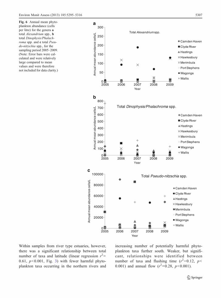
Large scale. For the eight key production areas, themean monthly phytoplankton abundance data (aver-aged across all years for taxa groupings ‘TotalAlexandrium spp.’, ‘Total Dinophysis/Phalachromaspp.’ and ‘Total Pseudo-nitzschia spp.’) showed phy-toplankton abundance to be highly variable acrossmonths but often with a winter/spring minimum(Fig. 5a–c). Interannual abundances were also variablefor these taxa groups, with no clear pattern emerging(Fig. 6a–c). The total number of potentially harmfultaxa occurring each year across all estuaries variedlittle among years, with 37 taxa identified in 2005,38 in 2006, 39 in 2007, and 40 for 2008 and 2009.
Small scale. Of the 31 estuaries investigated, 21estuaries showed significant differences among seasons
Fig. 4 Multivariate dendrogram showing the hierarchical clustering structure of NSW oyster-growing estuaries based on each estuary’sharmful phytoplankton abundance data (square root transformed). All sites, seasons and years have been pooled within each estuary
Tot
al n
umbe
r of
Phy
topl
ankt
on T
axa
S N
0
5
10
15
20
25
30
35
40
45Fig. 3 Total number ofharmful (toxic and related)taxa observed in water sam-ples collected by latitudinallocation (2005–2009) (tri-angles0rivers, R200.61,*p00.0001; circles0lakes;R200.02, p00.63, ns).
5304 Environ Monit Assess (2013) 185:5295–5316
for abundance data and 24 for taxa richness (Table 4).The Tweed, Clarence, Wooli Wooli (only sampled inspring and summer), Bellinger/Kalang and MacleayRivers showed no significant difference in phytoplanktonabundance between seasons while Wooli Wooli andBellinger rivers showed no significant difference in phy-toplankton taxa richness between seasons. The speciescontributing to the dissimilarity among seasons(SIMPER analysis) showed some similar patterns: (1)the P. delicatissima group frequently bloomed in sum-mer, autumn and spring with a winter minimum (exceptin Wallis Lake, Jervis Bay, Brisbane Water andWagongaInlet); (2) Pseudo-nitzschia seriata group (Pseudo-nitz-schia pungens\multiseries, Pseudo-nitzschia heimii
\subpacifica and Pseudo-nitzschia fraudulenta\australis)were usually highest in abundance in spring and lowest inwinter (except the Manning River, which had a highaverage abundance of P. pungens\multiseries in winter;and Jervis Bay, which had a high abundance of P. heimii\subpacifica in autumn); (3) Dinophysis caudata waspresent in all seasons, but relatively rare in winter, (al-thoughD. acuminata showed no clear seasonal patterns);(4) P. cordatum was generally in higher abundance inautumn/winter (except in the Manning River); (5)Prorocentrum rhathymum and Prorocentrum limawere more common in spring and less common inautumn and winter; (6) Takyama cf. pulchella andAlexandrium pseudogonyaulax were more often
Table 3 ANOSIM pairwise tests (square root, Bray-Curtis) and SIMPER results for sites within estuaries using harmful abundancephytoplankton data (square root transformed)
Estuary name ANOSIM for sites SIMPER
Estuaries with “dispersed” sites
Nambucca River U D P. delicatissima gp, P. cordatum, D. acuminata
Macleay River UU D P. delicatissima gp
Hastings River U DD P. delicatissima gp, D. acuminata
Camden Haven River UDD NA
Manning River UDD NA
Port Stephens UUU DD DDDDD P. delicatissima gp, P. pungens\multiseries, D. acuminata, D.octonaria, A. sanguínea
Brisbane Water UUU D D P. delicatissima gp, P. pungens\multiseries
Hawkesbury River UUD D P. delicatissima gp, P. cordatum, P. pungens\multiseries
Clyde River U D D P. delicatissima gp, D. octonaria, P. cordatum
Wagonga Inlet U D P. delicatissima gp
Estuaries with “aggregated” sites
Tweed River DD NA
Wallis Lake DDD NA
Hunter River DD NA
Shoalhaven/Crookhaven DDDD NA
Tuross River DD NA
Wapengo Lagoon D D P. delicatissima gp, P. fraudulenta\australis
Nelson Lake/Lagoon DD NA
Merimbula Lake D D P. delicatissima gp, P. cordatum
Pambula River DD NA
Twofold Bay DDDD NA
Wonboyn River D D P. delicatissima gp, P. cordatum
Estuaries with single sites are not shown. SIMPER analysis identified species with >50 % cumulative contribution to dissimilarityamong sites. Underlined sites are not significantly different (p≥0.05)NA not applicable since site differences were found to be not significant, U upstream: site in upper reaches of estuary approximately>6 km from estuary entrance, D downstream: site in lower reaches of estuary approximately <6 km from estuary entrance
Environ Monit Assess (2013) 185:5295–5316 5305
seen in spring than any other season; (7) Akashiwosanguínea showed no clear seasonal pattern al-though it was relatively more abundant in autumnin Port Stephens and in summer in WapengoLagoon.
Potential explanatory variables
Large scale. The regression between latitude andnumber of taxa for lakes (which included drownedvalleys) was not significant (r200.06, p>0.05).
100
200
300
400
500
600
700
800
Mo
nth
ly m
ea
n a
bu
nd
an
ce c
ells
/L
100
150
200
250
300
Mo
nth
ly m
ea
n a
bu
nda
nce
ce
lls/L
6
100000
Mon
thly
me
an a
bund
ance
ce
lls/L
0
0
50
0
20000
40000
60000
80000
M
Total Dinophysis/Phalachroma spp.
Month
Total Alexandrium spp.
Total Pseudo-nitzschia spp.
1 2 3 4 5 6 7 8 9onth
1 2 3 4 5 6 7 8 9
1 2 3 4 5 6 7 8 9Month
10 11 12
10 11 12
10 11 12
Camden H
Clyde
Hastings
Hawkesbu
Merimbula
Port Steph
Wagonga
Wallis
Camden H
Clyde
Hastings
Hawkesb
Merimbul
Port Steph
Wagonga
Wallis
Camden H
Clyde
Hastings
Hawkesbu
Merimbul
Port Steph
Wagonga
Wallis
Haven
ury
a
hens
Haven
ury
a
hens
a
Haven
ury
a
hens
a
a
b
c
Fig. 5 Monthly mean phy-toplankton abundance (cellsper litre) for the genera atotal Alexandrium spp., btotal Dinophysis/Phalach-roma spp. and c total Pseu-do-nitzschia spp., for thesampling period 2005–2009;austral winter0months 6–8.(Note: Error bars were cal-culated and were relativelylarge compared to meanvalues and were thereforenot included for data clarity.)
5306 Environ Monit Assess (2013) 185:5295–5316
Within samples from river type estuaries, however,there was a significant relationship between totalnumber of taxa and latitude (linear regression r200.61, p<0.001, Fig. 3) with fewer harmful phyto-plankton taxa occurring in the northern rivers and
increasing number of potentially harmful phyto-plankton taxa further south. Weaker, but signifi-cant, relationships were identified betweennumber of taxa and flushing time (r200.12, p<0.001) and annual flow (r200.28, p<0.001).
0
50
100
150
200
250
300
2005 2006 2007 2008 2009
An
nu
al m
ea
n a
bu
nd
an
ce c
ells
/L
Year
Camden Haven
Clyde River
Hastings
Hawkesbury
Merimbula
Port Stephens
Wagonga
Wallis
Total Alexandrium spp.
0
100
200
300
400
500
600
700
800
2005 2006 2007 2008 2009
An
nu
al m
ea
n a
bu
nd
an
ce c
ells
/L
Year
Camden Haven
Clyde River
Hastings
Hawkesbury
Merimbula
Port Stephens
Wagonga
Wallis
Total Dinophysis/Phalachroma spp.
0
20000
40000
60000
80000
100000
2005 2006 2007 2008 2009
An
nu
al m
ea
n a
bun
da
nce
ce
lls/L
Year
Camden Haven
Clyde River
Hastings
Hawkesbury
Merimbula
Port Stephens
Wagonga
Wallis
Total Pseudo-nitzschia spp.
a
b
c
Fig. 6 Annual mean phyto-plankton abundance (cellsper litre) for the genera atotal Alexandrium spp., btotal Dinophysis/Phalach-roma spp. and c total Pseu-do-nitzschia spp., for thesampling period 2005–2009.(Note: Error bars were cal-culated and were relativelylarge compared to meanvalues and were thereforenot included for data clarity.)
Environ Monit Assess (2013) 185:5295–5316 5307
Small scale. There was no significant differencein phytoplankton abundance among bioregions,(global test, ANOSIM p<0.05) (Table 5). Therewas, however, a significant effect of bioregionson number of taxa (global test, ANOSIM p>0.05); significant pair-wise tests revealed an in-crease in species occurrence in southern estuaries(Table 5). Common genera which contributed to thedissimilarity between bioregions were the dinoflagel-lates Alexandrium, Phalachroma and Prorocentrumwhich occurred more frequently in the southern estuar-ies. Significant separationwas also seen for estuary class(rivers, lakes) with greater numbers of taxa in lakescompared to rivers (Table 5).
Phytoplankton abundance was significantlylinked with flushing—those estuaries with shortflushing times (i.e. rapid turnover of water) hadlower abundance of the common genus Pseudo-nitzschia compared to those with medium flushingrates. Number of taxa, however, was not affectedby flushing (Table 5).
Estuary modification levels significantly correlatedwith phytoplankton abundance (global test, ANOSIMp>0.05), with pairwise tests revealing largely unmod-ified estuaries separated from modified and extremelymodified estuaries. P. delicatissima gp, P. cordatumand Pseudo-nitzschia fraudulenta/australis had higherpercentage abundance in modified estuaries, followed
Table 4 Significant pairwisetests for seasons within estuaries(analyses of similarity ANO-SIM) using harmful phytoplank-ton abundance (square-roottransformed) and species rich-ness (presence/absence trans-formed) data
Underlined seasons are not sig-nificantly different from eachother but are in no particular or-der (p≥0.05)S summer (December–Febru-ary), A autumn (March–May),W winter (June–August), SPspring (September–November)
Harmful phytoplanktonabundance
Harmful phytoplanktonrichness
Estuary ANOSIM ANOSIM
Tweed SP S AW
Richmond River SP S AW SP S AW
Clarence River W SP S A
Kalang River SP S AW
Nambucca River W S A SP W S A SP
Macleay River SP S AW
Hastings River S AW SP AW S SP
Camden Haven River S AW SP AW SP S
Manning River SP S AW S AW SP
Wallis A W S SP SP S WA
Port Stephens S A SP W S AW SP
Hunter River A S W SP
Brisbane Water S AW SP S AW SP
Patonga SP A S W S AW SP
Hawkesbury River S AW SP S AW SP
Georges River S AW SP SP W S A
Shoalhaven/Crookhaven S AW SP S AW SP
Jervis Bay S AW SP S AW SP
Conjola Lake W S A SP W S A SP
Clyde River SP S AW SP S AW
Tuross River S AW SP S AW SP
Wagonga Inlet A W SP S S AW SP
Bermagui River S AW SP S AW SP
Wapengo Lagoon S AW SP S AW SP
Nelson Lagoon S AW SP S AW SP
Merimbula Lake S AW SP S AW SP
Pambula River S AW SP S AW SP
Twofold Bay S W SP A S AW SP
Wonboyn River S AW SP S AW SP
5308 Environ Monit Assess (2013) 185:5295–5316
by extremely modified estuaries and lowest in largelyunmodified estuaries. Furthermore, estuary modifica-tion level showed significant pairwise tests for numb-ers of taxa. Largely unmodified estuaries separatedfrom modified and in turn with extremely modifiedestuaries, with the largely unmodified estuaries show-ing greatest numbers of HAB species (Table 5).
No significant differences among estuaries (for eitherabundance or number of taxa) were found for the poten-tial explanatory variables dilution, estuary subclass, totalsuspended solids ratio, total phosphorus index or totalnitrogen index (Table 5).
Phytoplankton action limits
Phytoplankton action limits (PALs) were exceededat 86 % sites and for 20 phytoplankton taxa (andfour total genera groupings) during the samplingperiod (Table 2). Wagonga Inlet and Wallis Lakewere assessed as having the highest risk of
potentially harmful algal blooms with the greatestoverall number of exceedances for any estuary (themajority of these exceedances were due to the‘Total Pseudo-nitzschia’ group). Across all estuar-ies, the PAL for ‘Total Alexandrium’ was exceededin 126 samples (47 due to A. catenella/fundyenseand 52 due to A. pseudogonyaulax). ‘TotalDinophysis/Phalachroma’ exceeded the PAL in136 samples (58 samples exceeded for D. acumi-nata) and 310 samples exceeded the PAL for ‘TotalPseudo-nitzschia’ (54 for P. delicatissima; 34 for P.fraudulenta/australis, 53 for P. multiseries/australisand 18 for P. pungens/multiseries). Months withsamples that exceeded the PALs varied among estu-aries, although the majority of PAL exceedancesoccurred in spring, summer and autumn while aminimum was generally noted in winter (NSWFood Authority 2011).
Thirteen estuaries experienced shellfish harvest-ing closures (total number closures034) during the
Table 5 ANOSIM global significance (R) and pairwise test results between estuaries for external factors
0.001 M vs LU 0.107 0.001* 0.002 M vs EM 0.049 0.023*
EM vs LU 0.045 0.024* M vs LU 0.067 0.001*
EM vs LU 0.064 0.005*
Due to low sample size Wooli Wooli River, Jervis Bay and Lake Conjola were not included
ns not significant
*p<0.05 significant
Environ Monit Assess (2013) 185:5295–5316 5309
sampling period due to algal blooms, with theHawkesbury River having the greatest number ofclosures (n013). Positive toxin tests were recordedfor 12 estuaries over the sampling period: 20 pos-itive toxin tests for paralytic shellfish poisoning(PSP); and six positive toxin tests for amnesicshellfish poisoning (ASP). The Hawkesbury estu-ary had the greatest number of toxic events duringthis time (n06) with all of these being PSP posi-tive (NSW Food Authority 2011).
Discussion
Spatial patterns in harmful phytoplankton richnessand abundance
From a broad spatial perspective, the majority of the45 potentially harmful taxa identified in New SouthWales estuaries belong to the genera Pseudo-nitzschia(species belonging to this group are the causative taxaof amnesic shellfish poisoning), Dinophysis/Phalachroma, Prorocentrum (diarrhetic shellfish poi-soning) and Gymnodinium and Alexandrium (paralyticshellfish poisoning). These genera have commonlybeen found in other harmful algal monitoring pro-grams throughout the world (Hernandez-Becerril etal. 2007; Vershinin and Orlova 2008). Distinct biore-gional differences in species richness were observed inour study; however, and within this pattern, a distinctgradient in harmful species richness from north tosouth for rivers was revealed. Harmful species rich-ness was lowest in the northern bioregions (Tweed-Moreton) where warm temperate/subtropical watersprevail, and increased southward (Twofold Shelf),where cool temperate waters dominate. The major-ity of riverine estuaries in the north are largebarrier rivers, with variable flushing times andlow nutrient retention rates. Alternatively, the par-tially mixed temperate systems in the south areable to trap, accumulate and reprocess nutrientsas well as provide variable habitat and salinityregimes which may account for the maximum spe-cies diversity observed.
If we consider temperature as a major driving factorfor the patterns observed (lower species richness in thenorth), we could hypothesise that with climate warm-ing, changes may occur in community compositionand/or biogeographical range contractions of HAB
taxa along the NSW coastline. A shift in the dominanttoxin-producing algal species in central California hasalready altered the phycotoxins in the pelagic foodweb of this ecosystem. Although not conclusive, thisshift from a diatom-dominated community to red tide,dinoflagellate-dominated community has been linkedto basin-scale climate warming (Jester et al. 2009).Alternatively, an increase in the poleward extensionof the East Australian current, the dominant westernboundary current along the NSW coast (Thompson etal. 2009), may increase the geographic range of certainspecies into more southern waters. In support of thishypothesis, a range extension of the tropical speciesGambierdiscus cf. toxicus in eastern Australianwaters, from Brisbane (25°S) to Merimbula (36.5°S),has been reported in recent years (Hallegraeff 2010).The movement of this particular species is furthersupported by our data, which indicates a southwardextension to Wonboyn (37 °S). Similar to this rangeextension, there exists the real potential for otherharmful tropical genera, such as Pyrodinium to extendinto more southern Australian waters. Globally, how-ever, it is reported that some species have increasedtheir habitat range from tropical and temperate latitudesto colder environments whilst certain coldwater assemb-lages are retracting to higher latitudes (see review,Hallegraeff 2010). A species ecological response toclimate warming will be dependent on its individualaffinity to temperature in combination with an array ofother driving influences.
The disparity observed between species richnessamong estuaries is likely, however, to be a result ofcomplex interactions between environmental factorssuch as temperature and others, such as, resourcesupply (inorganic nutrients and micronutrients fromeither oceanic sources or catchment runoff), estuarycharacteristics (rainfall, salinity, flushing time, distur-bance level, etc.) and zooplankton grazing effects(Sunda and Shertzer 2012). Recent laboratory studiesfor Pseudo-nitzschia, for example, have shown thatmost species belonging to this genus are both euryha-line and halotolerant (see review, Lelong et al. 2012).Lelong et al. (2012) stress, however, that althoughthe salinity ranges examined in laboratory studiesare broader than those found in the environmentand that these kinds of experiments can be con-founded by other variables such as temperatureand species-specific requirements. The authorsconclude that despite this complexity, salinity
5310 Environ Monit Assess (2013) 185:5295–5316
remains an important variable in the growth andpersistence of Pseudo-nitzschia. Unfortunately, re-liable salinity data were not available for examina-tion in the present study, but its importance isparamount for any future, smaller-scale HAB stud-ies in these estuaries.
The most consistent pattern in harmful speciesabundance (and richness) observed within estuarieswas an upstream/downstream zonation. Pseudo-nitz-schia spp., D. acuminata and D. octonaria generallyfavoured the more marine, dynamic tidal zone of es-tuaries while the abundance of P. cordatum favouredthe central, mud basin/fluvial delta of the estuarysystem. Whilst Pseudo-nitzschia growth can occuracross a broad range of salinities (6–48 psu) andtemperatures (5–30 °C), Pseudo-nitzschia blooms areoften triggered by riverine input of nutrients, coastalnutrient upwellings and the provision of coastal sili-cate for frustule biosilicification (Trainer et al. 2012).Similarly, D. octonaria shows optimal growth at sal-inities of 15–25 % within a temperature range of 11–15 °C, but blooms are often triggered by the supply ofseed populations from oceanic waters (Henriksen et al1993; Rigual-Hernandez et al. 2010). With only therecent capability to culture D. acuminata, light, preyavailability and continental shelf seeding are consid-ered the most important factors in their bloom initia-tion (Reguera et al. 2012). In contrast, the significantlyhigher abundance (and occurrence) of P. cordatum atupstream sites is most likely due to its ability to act asa eutrophication indicator, having a high growth rateunder high nutrient conditions. It can also demon-strates a high physiological flexibility, having a hightolerance for changing environmental parameters (light,temperature, salinity) and a capacity to store nutrientsand reuse them under low nutrient availability (Fan et al.2003, Fan and Glibert 2005; Heil et al. 2005; Glibert etal. 2008a, 2012; Li et al. 2011). Many other harmfulProrocentrum spp. identified in our study have a benthicassociation (P. concavum, P. emarginatum and P. lima).Based on the hydrological attributes of upstream harvestareas, we suggest that this group of benthic microalgaewould similarly favour this habitat. A more detailedanalysis of these two groups of species is the focus ofa future study.
Nutrient condition and intensity of turbulencehave been identified as key factors in controllingthe morphotaxonomy, physiology and ecologicalniches of harmful phytoplankton (Margalef 1978).
Extending this model along an onshore–offshoregradient (decreasing nutrients, reduced mixing,deepening euphotic zone and a consideration oflife form “traits”), harmful bloom-forming dinofla-gellates have been categorised into nine groupseach with distinct morphological features coupledto habitat preference (Smayda and Reynolds 2001,2003). This model was not designed for the up-stream reaches of estuaries, nor included diatoms,but with more careful analysis of harmful speciespartitioning, this ecological niche hypothesis couldbe tested for estuarine environments.
If we then consider estuary disturbance (or nichedisruption) as a major driver of species richness, in-creased species richness would be expected to occur inestuaries which are more stable, unmodified and havehigher residence times (favouring k-selected organ-isms such as dinoflagellates), compared to those thatare less stable, highly disturbed and have lower resi-dence times (flavouring r-selected organisms such asdiatoms). This pattern of species density is supportedby our data, although, a more focussed description ofniche width in these estuaries would be essential forthe prediction of niche expansion or conversely, nichecontraction.
Temporal patterns in harmful phytoplankton richnessand abundance
In the current study, it has been assumed that samplestaken at fortnightly intervals are statistically indepen-dent, but this is an assumption that needs much greaterscrutiny in the future given the potential for serialcorrelation in phytoplankton counts taken over a peri-od of days to weeks. Daily samples over a period ofmonths to years would, however, be required to testsuch an assumption, and the data to do such testingdoes not currently exist. The potential for serial corre-lation to affect interpretations from statistical tests,nevertheless, needs to be acknowledged here.
When the wide range of estuarine ecosystems in-vestigated in our study is considered, it is not surpris-ing that complex temporal patterns emerged. Whilethere is considerable disparity among seasons acrossestuaries, some consistent seasonal patterns were sug-gested providing useful observations on some risktaxa. The P. delicatissima group was generally highestin abundance in autumn, summer and spring, thePseudo-nitzschia seriata group generally highest in
Environ Monit Assess (2013) 185:5295–5316 5311
spring, and P. cordatum was more abundant in autumnand winter. The seasonality of Pseudo-nitzschia innorthern hemisphere waters has been demonstrated,with non-toxic P. delicatissima dominating the delica-tissima group in spring, and the seriata group occur-ring mainly during the summer months (Fehling et al.2006). Pseudo-nitzschia blooms, in other regions ofthe world, however, do not support such a seasonalpattern, demonstrating complex, species dynamics thatare often regionally specific (Trainer et al. 2012).
From a global perspective, temporal variability ofphytoplankton abundance and diversity can occur at avariety of scales from the short-term (days, weeks) tothe longer-term (months, seasons and years). Theymay also be associated with prevailing climatic con-ditions (e.g. ENSO, upwelling). When 114 estuaries,lagoons, inland seas, bays and shallow coastal watersaround the world were investigated for their time-series of phytoplankton biomass, a broad continuumof seasonal patterns was revealed (Cloern and Jassby2010). These authors found that local factors such asupwelling events, riverine inputs, tidal cycles, weatherevents and flushing times were the dominant processescausing the observed variability. Whilst a proportionof the variability in phytoplankton abundance may bepredictable (e.g. seasonal peaks in abundance/occur-rence), there is still a great deal of unexplained varia-tion in phytoplankton abundance (Lucas and Cloern2002; Kromkamp and Engeland 2010; Zingone et al.2010). Although our results provide some broadpatterns regarding risk taxa and their seasonal dis-tributions, there is still much to be learned aboutpotentially toxic phytoplankton abundance andcomposition in NSW estuaries. Further estuary-specific and longer-term studies will be necessaryto understand the link between local drivers andany seasonal patterns within specific estuaries.
Potential explanatory variables
Estuary modification level and flushing rates wererevealed as having the highest association with harm-ful phytoplankton biomass among estuaries. Speciesrichness patterns also revealed significant links tobioregion, estuary class and estuary modification level(discussed previously). Consistent with internationalfindings, research in NSW estuaries has demonstratedthat increased nutrient loading to estuaries promotedincreased algal biomass (measured as chlorophyll a,
Scanes et al. 2007). NSW estuaries are also particular-ly sensitive to nutrient inputs, and significant chloro-phyll concentrations have been induced at nitrogenloadings up to an order of magnitude less than thosein comparable northern hemisphere situations. It is ofinterest to note that in our study (which included manyof the same estuaries as Scanes et al. 2007), there wasno relationship between harmful algal composition orbiomass and increased nutrient loading. This has twoimportant implications. Firstly, the heterotrophic na-ture of many of the harmful algal species may explaintheir poor correlation with nutrient inputs and, as acorollary, this may mean that algal assessments basedon chlorophyll a are inadequate to assess the risk ofharmful algal blooms. Secondly, the nutrient assimila-tion potential of an estuary is influenced by nutrientdelivery coupled with water residence time (Phlips etal. 2011; Rissik et al. 2006). In this regard, there is aneed for significantly more consideration of the inter-active effects of factors such as physico-chemistry(salinity, temperature, etc.), nutrient enrichment,species-specific ecology, trophic interactions andphysical processes, all of which may result in a com-plex range of phytoplankton responses (Cloern 2001;Leibold et al. 2004; Davis and Koop 2006; Glibert etal. 2008b, 2011; Heisler et al. 2008, Macintyre et al.2011).
Other external variables that did not demonstrate asignificant link with harmful phytoplankton abun-dance were bioregion, estuary class or estuary sub-class. Classification systems developed for NewSouth Wales estuaries have historically been basedon geomorphology, salinity, or hydrology and onlyrecently included response-, functional- andbioregionalisation-based approaches (Roy et al.2001; Roper et al. 2011). Using a combination of theseclassification schemes, conceptual models are nowbeing developed for some NSW estuaries. While thesemodels are currently undergoing validation, it is rec-ognized that individual estuaries, with varying depthprofiles, entrance conditions, salinity and temperaturegradients, and catchment characteristics may still varyfrom generic classifications commonly used to de-scribe the condition of an estuary (Roper et al. 2011).Further refinement of these estuary classifications us-ing quantitative phytoplankton community data suchas presented in this study, may help improve thesemodels and provide an improved tool for the manage-ment of aquatic ecosystems.
5312 Environ Monit Assess (2013) 185:5295–5316
Harmful algal bloom risk assessment
Comparison of phytoplankton cell densities with phyto-plankton action limits (PALs) highlighted the individualtaxa zones of risk in the oyster-growing estuaries ofNew South Wales (Wallis Lake, Wagonga Inlet andHawkesbury River). Both the Hawkesbury River andWallis Lake estuaries have degraded water quality, re-duced flow and highly developed land use (http://www.ozcoasts.gov.au). These estuary modification var-iables most likely combine to cause the retention ofnutrients and reduced water exchange favouring theproliferation of tolerant harmful algal species (Roy etal. 2001; Figueiras et al. 2006). On the other hand,Wagonga Inlet is a relatively unimpacted estuary, al-though different forcing variables such as sedimenta-tion, sewage/stormwater runoff and entrance channelshoaling, may trigger the excess growth of residentharmful species.
The prevalence of risk taxa (Pseudo-nitzschia,Alexandrium and Dinophysis) revealed in this studyhighlight the continued need for rigorous biotoxinmonitoring in the oyster-growing estuaries of NewSouth Wales. PALs are based on the most up-to-dateknowledge of harmful phytoplankton worldwide, andwhile there has been significant advances relating toestuarine and catchment modeling in Australian coast-al aquatic ecosystems, there is a very limited under-standing of phytoplankton ecology, toxicology andtaxonomy in local waters (Davis and Koop 2006).This is reflected in the disparity between the numberof exceedances (many hundreds) and resultant bio-toxic events (26), and our inability to forecast orpredict the relationship between phytoplankton cellconcentrations and the toxin levels that may emergein shellfish (Takahashi et al. 2007).
One of the key genera, Pseudo-nitzschia is a cosmo-politan genus found worldwide in polar, temperate, sub-tropical and tropical waters (Hasle 2002; Trainer et al.2012). It has also been observed in the coastal waters ofall states of Australia (Hallegraeff 1994; Lapworth et al.2001). Despite its worldwide prevalence and signifi-cance in NSW estuaries as revealed in our study, therehas been no investigation into the link between localPseudo-nitzschia strains and toxin (domoic acid) produc-tion in our coastal waters, and no inter- or intra-specificmolecular examination among Pseudo-nitzschia strains.In addition, both toxic and non-toxic forms ofPseudo-nitzschia cannot be distinguished using
light microscopy and require electron microscopyconfirmation. Action limits for risk minimizationfor this genera is currently based on “total Pseudo-nitzschia” or the “P. delicatissima group”, butwithout the resolution of the genera and group tospecies level, it is most likely that many shellfishharvest area closures are occurring unnecessarily.As further information emerges about harmful al-gal taxa and human health impacts, it is expectedthat these action limits will be refined for theAustralian setting.
Conclusions
Our study provides the first major synthesis of poten-tially harmful phytoplankton in the oyster-growingestuaries of eastern Australia. Species richness waslatitudinally graded for rivers, with increasing numberof taxa southward. A consistent upstream versusdownstream pattern emerged in both compositionand abundance within estuaries. Species abundancecorrelated to estuary modification levels and flushingtime, with modified, slow flushing estuaries havingincreased abundance. Species richness correlated withbioregion, estuary modification levels and estuaryclass, with southern, unmodified lakes demonstratinggreater species density.
Differences in phytoplankton abundance and compo-sition between bioregions, estuary type, level of catch-ment disturbance and within-estuary variability, callattention to the need for careful site/estuary selectionwhen considering future aquaculture operations andbiotoxin monitoring programs. The extent to whichother biotoxin monitoring studies worldwide have beenundertaken, that is, to meet management criteria formonitoring shellfish harvest areas, has usually driventhe focus of studies to compile harmful species check-lists, bloom occurrence rates and toxicity informationrelating to human health. Rarely has the spatial or tem-poral distribution patterns of harmful taxa been scruti-nised. Phlips et al. (2011), using a similar monitoringeffort, developed a statistical approach to estimating theprobability of detecting HAB events for key species.The power of such an approach was limited bysampling intervals utilised, although the authorsconcluded that with longer datasets and a greaterunderstanding of species- and ecosystem-specificpressures, this forecast ability would improve.
Similarly, the distinctly observational nature of ourstudy, with its inherent limitations such as sam-pling frequency and site selection, is a worthy casestudy in the examination of potentially harmfulphytoplankton dynamics, which will value-add tofuture aquaculture proposals and estuary modeldevelopment. With appropriately scaled estuary-and species-specific process studies we may fur-ther elucidate the mechanisms underlying phyto-plankton distribution and bloom drivers. With thisinformation, we may improve our ability to makereliable predictions on future trends in risk taxaand risk zones.
Acknowledgments The authors would like to thank AnthonyZammit (NSW Food Authority), Mr. Jamie Potts (NSW Officeof the Environment and Heritage), Dr. Shauna Murray (Univer-sity of New South Wales), Dr. Ana Rubio (University of Wol-longong) and Professor Gustaaf Hallegraeff (University ofTasmania) for the useful discussions throughout this study. Thiswork was supported by an Australian Postgraduate Award, NewSouth Wales Food Authority and the Australian Government’sAustralian Biological Resource Study (CT210-19).
References
Anderson, D. M., Burkholder, J. M., Cochlan, W. P., Glibert, P.M., Gobler, C. J., Heil, C. A., et al. (2008). Harmful algalblooms and eutrophication: examining linkages from se-lected coastal regions of the United States. Harmful Algae,8(1), 39–53.
Clarke, K.R., & Warwick, R.M. (2001). Change in marine com-munities: an approach to statistical analysis and interpreta-tion. 2nd edition: PRIMER-E. (pp. 1–172). Plymouth, UK.
Cloern, J. E. (2001). Our evolving conceptual model of thecoastal eutrophication problem. Marine Ecology-ProgressSeries, 210, 223–253.
Cloern, J. E., & Jassby, A. D. (2010). Patterns and scales ofphytoplankton variability in estuarine-coastal ecosystems.Estuaries and Coasts, 33(2), 230–241.
Davis, J. R., & Koop, K. (2006). Eutrophication in Australianrivers, reservoirs and estuaries—a southern hemisphereperspective on the science and its implications. Hydrobio-logia, 559, 23–76.
Falkowski, P. G., Barber, R. T., & Smetacek, V. (1998). Bio-geochemical controls and feedbacks on ocean primaryproduction. Science, 281, 200–206.
Fan, C., & Glibert, P. M. (2005). Effects of light on nitrogen andcarbon uptake during a Prorocentrum minimum bloom.Harmful Algae, 4(3), 629–641.
Fan, C., Glibert, P. M., & Burkholder, J. M. (2003). Character-ization of the affinity for nitrogen, uptake kinetics, and
environmental relationships for Prorocentrum minimumin natural blooms and laboratory cultures. Harmful Algae,2(4), 283–299.
Fehling, J., Davidson, K., Bolch, C., & Tett, P. (2006). Season-ality of Pseudo-nitzschia spp. (Bacillariophyceae) in west-ern Scottish waters. Marine Ecology-Progress Series, 323,91–105.
Figueiras, F.G., Pitcher, G.C., Estrada, M. (2006). Harmful algalbloom dynamics in relation to physical processes. In Gra-néli, E. and Turner, J.T. (Eds) Ecology of harmful algae.Springer, pp. 127-138.
Fritz, L., & Triemer, R. E. (1985). A rapid simple techniqueutilizing calcofluor white M2R for the visualization ofdinoflagellate thecal plates. Journal of Phycology, 21(4),662–664.
Glibert, P. M., Burkholder, J. M., Graneli, E., & Anderson, D.M. (2008). Advances and insights in the complex relation-ships between eutrophication and HABs: preface to thespecial issue. Harmful Algae, 8(1), 1–2.
Glibert, P. M., Mayorga, E., & Seitzinger, S. (2008). Prorocen-trum minimum tracks anthropogenic nitrogen and phospho-rus inputs on a global basis: application of spatially explicitnutrient export models. Harmful Algae, 8(1), 33–38.
Glibert, P. M., Fullerton, D., Burkholder, J. M., Cornwell, J. C.,& Kana, T. M. (2011). Ecological stoichiometry, biogeo-chemical cycling, invasive species, and aquatic food webs:San Francisco estuary and comparative systems. Reviewsin Fisheries Science, 19(4), 358–417.
Glibert, P. M., Burkholder, J. M., & Kana, T. M. (2012).Recent insights about relationships between nutrientavailability, forms, and stoichiometry, and the distribu-tion, ecophysiology, and food web effects of pelagicand benthic Prorocentrum species. Harmful Algae, 14,231–259.
Hallegraeff, G. M. (1993). A review of harmful algal blooms andtheir apparent global increase. Phycologia, 32(2), 79–99.
Hallegraeff, G. M. (1994). Species of the diatom genus Pseudo-nitzschia in Australian Waters. Botanica Marina, 37(5),397–412.
Hallegraeff, G. M. (2010). Ocean climate change, phytoplank-ton community responses, and harmful algal blooms: aformidable predictive challenge. Journal of Phycology, 46(2), 220–235.
Hallegraeff, G. M., Anderson, D. M., & Cembella, A. D. (Eds.).(2003). Manual on harmful marine microgalgae (p. 793).Paris: UNESCO Publishing.
Hasle, G. R. (2002). Are most of the domoic acid-producingspecies of the diatom genus Pseudo-nitzschia cosmopo-lites? Harmful Algae, 1(2), 137–146.
Heil, C. A., Glibert, P. M., & Fan, C. (2005). Prorocentrumminimum (Pavillard) Schiller: a review of a harmful algalbloom species of growing worldwide importance. HarmfulAlgae, 4(3), 449–470.
Heisler, J., Glibert, P. M., Burkholder, J. M., Anderson, D. M.,Cochlan, W., & Dennison, W. C. (2008). Eutrophicationand harmful algal blooms: a scientific consensus. HarmfulAlgae, 8(1), 3–13.
Henriksen, P., Knipschildt, F., Moestrup, Ø., & Thomsen, H. A.(1993). Autecology, life history and toxicology of thesilicoflagellate Dictyocha speculum (Silicoflagellata, Dic-tyochophyceae). Phycologia, 32(1), 29–39.
5314 Environ Monit Assess (2013) 185:5295–5316
Hernandez-Becerril, D. U., Alonso-Rodriguez, R., Alvarez-Gongora, C., Baron-Campis, S. A., Ceballos-Corona, G.,Herrera-Silveira, J., et al. (2007). Toxic and harmful marinephytoplankton and microalgae (HABs) in Mexican Coasts.Journal of Environmental Science and Health Part a-Toxic/Hazardous Substances & Environmental Engineer-ing, 42(10), 1349–1363.
Hill, M. O. (1973). Diversity and evenness: a unifying notationand its consequences. Ecology, 54(2), 427–432.
Integrated Marine and Coastal Regionalisation of Australia(IMCRA), 2011. http://www.environment.gov.au/coasts/mbp/imcra/index.html
Jester, R., Lefebvre, K., Langlois, G., Vigilant, V., Baugh, K., &Silver, M. W. (2009). A shift in the dominant toxin-producing algal species in central California alters phyco-toxins in food webs. Harmful Algae, 8(2), 291–298.
Kromkamp, J. C., & Van Engeland, T. (2010). Changes in phyto-plankton biomass in the Western Scheldt estuary during theperiod 1978-2006. Estuaries and Coasts, 33(2), 270–285.
Lapworth, C., Hallegraeff, G.M., & Ajani, P.A. (2001). Identi-fication of domoic-acid producingPseudo-nitzschia speciesin Australian waters. In G. M. Hallegraeff, Blackburn, S.I.,Bolch, C.J. and Lewis, R.J. (eds) (Ed.), Harmful algalblooms 2000 (pp. 39-42): Intergovernmental Oceanograph-ic Commission of UNESCO 2001.
Leibold, M. A., Holyoak, M., Mouquet, N., Amarasekare, P.,Chase, J. M., Hoopes, M. F., et al. (2004). The metacom-munity concept: a framework for multi-scale communityecology. Ecology Letters, 7(7), 601–613.
Lelong, A., Hégaret, H., Soudant, P., & Bates, S. S. (2012).Pseudo-nitzschia (Bacillariophyceae) species, domoic acidand amnesic shellfish poisoning: revisiting previous para-digms. Phycologia, 51(2), 168–216.
Li, Y., Lü, S., Jiang, T., Xiao, Y., & You, S. (2011). Environ-mental factors and seasonal dynamics of Prorocentrumpopulations in Nanji Islands National Nature Reserve, EastChina Sea. Harmful Algae, 10(5), 426–432.
Lucas, L. V., & Cloern, J. E. (2002). Effects of tidal shallowingand deepening on phytoplankton production dynamics: amodeling study. Estuaries, 25(4A), 497–507.
Macintyre, H. L., Stutes, A. L., Smith, W. L., Dorsey, C.P., Abraham, A., & Dickey, R. W. (2011). Environ-mental correlates of community composition and tox-icity during a bloom of Pseudo-nitzschia spp. in thenorthern Gulf of Mexico. Journal of Plankton Re-search, 33(2), 273–295.
Margalef, R. (1978). Life-forms of phytoplankton as survivalalternatives in an unstable environment. Oceanology Acta,1, 493–509.
Moore, S. K., Trainer, V. L., Mantua, N. J., Parker, M. S., Laws,E. A., & Backer, L. C. (2008). Impacts of climate variabil-ity and future climate change on harmful algal blooms andhuman health. Environmental Health, 7. doi:10.1186/1476-069x-7-s2-s4.
National Land and Water Resources Audit (NLWRA) 2001.Australian Water Resources Assessment 2000 http://www.anra.gov.au/topics/water/pubs/national/water_contents.html
New South Wales Food Authority, 2011. http://www.foodauthority.nsw.gov.au/industry/industry-sector-requirements/shellfish
New South Wales Industry and Investment (NSW I & I), 2010.Aquaculture Production Report 2009-2010, 17 pp.
NSW Marine Biotoxin Management Plan (2011). NSW Shell-fish Program NSW/FA/FI115/1105, NSW Food Authority.
O’Connor W. A., Dove M. (2009). The changing face of oysterculture in New South Wales, Australia. Journal of ShellfishResearch, 28, 803–812.
Phlips, E. J., Badylak, S., Christman, M. C., & Lasi, M. A.(2010). Climatic trends and temporal patterns of phyto-plankton composition, abundance, and succession in theIndian River Lagoon, Florida, USA. Estuaries and Coasts,33(2), 498–512.
Phlips, E. J., Badylak, S., Christman, M. Wolny, J., Brame,J. Garland, J. Hall, L., Hart, J., Landsberg, J., Lasi, M.,Lockwood, J., Paperno, R., Scheidt, D., Staples, A.,Steidinger, K. (2011). Scales of temporal and spatial variabil-ity in the distribution of harmful algae species in the IndianRiver Lagoon, Florida, USA. Harmful Algae, 10, 277–290.
Pitcher, G. C. (2012). Harmful algae-the requirement forspecies-specific information. Harmful Algae, 14, 1–4.
Puigserver,M.,Monerris, N., Pablo, J., Alos, J., &Moya, G. (2010).Abundance patterns of the toxic phytoplankton in coastalwaters of the Balearic Archipelago (NW Mediterranean Sea):a multivariate approach. Hydrobiologia, 644(1), 145–157.
Reguera, B., Velo-Suárez, L., Raine, R., & Park, M. G. (2012).Harmful Dinophysis species: a review. Harmful Algae, 14,87–106.
Rhodes, R. H., Bertler, N. A. N., Baker, J. A., Sneed, S. B.,Oerter, H., & Arrigo, K. R. (2009). Sea ice variability andprimary productivity in the Ross Sea, Antarctica, frommethylsulphonate snow record. Geophysical Research Let-ters, 36, L10704. doi:10.1029/2009GL037311.
Rigual-Hernandez, A. S., Barcena, M. A., Sierro, F. J.,Flores, J. A., Hernandez-Almeida, I., Sanchez-Vidal,A., et al. (2010). Seasonal to interannual variabilityand geographic distribution of the silicoflagellatefluxes in the Western Mediterranean. Mar. Micropa-leontol., 77, 46–57.
Rissik, D., Doherty, M., & van Senden, D. (2006). A manage-ment focused investigation into phytoplankton blooms in asub-tropical Australian estuary. Aquatic Ecosystem Health& Management, 9(3), 365–378.
Roper, T., Creese, B., Scanes, P., Stephens, K., Williams, R.,Dela-Cruz, J., et al. (2011). Assessing the condition ofestuaries and coastal lake ecosystems in NSW. NSW Stateof the Catchments 2010 (p. 239). NSW: Office of Environ-ment and Heritage.
Roy, P. S., Williams, R. J., Jones, A. R., Yassini, I., Gibbs, P. J.,Coates, B., et al. (2001). Structure and function of south-east Australian estuaries. Estuarine, Coastal and ShelfScience, 53(3), 351–384.
Scanes, P., Coade, G., Doherty, M., & Hill, R. (2007). Evalua-tion of the utility of water quality based indicators ofestuarine lagoon condition in NSW, Australia. Estuarine,Coastal and Shelf Science, 74(1–2), 306–319.
Smayda, T. J., & Reynolds, C. S. (2001). Community assemblyin marine phytoplankton: application of recent models toharmful dinoflagellate blooms. Journal of Plankton Re-search, 23(5), 447–461.
Smayda, T. J., & Reynolds, C. S. (2003). Strategies of marinedinoflagellate survival and some rules of assembly. Journalof Sea Research, 49(2), 95–106.
Sunda, W. G., & Shertzer, K. W. (2012). Modeling ecosystemdisruptive algal blooms: positive feedback mechanisms.Marine Ecology Progress Series, 447, 31–47.
Takahashi, E., Yu, Q., Eaglesham, G., Connell, D. W.,McBroom, J., & Costanzo, S. (2007). Occurrence andseasonal variations of algal toxins in water, phytoplanktonand shellfish from North Stradbroke Island, Queensland,Australia. Marine Environmental Research, 64(4), 429–442.
Thomas, A. C., Weatherbee, R., Xue, H., & Liu, G. (2010).Interannual variability of shellfish toxicity in the Gulf ofMaine: time and space patterns and links to environmentalvariability. Harmful Algae, 9(5), 458–480.
Thompson, P. A., Baird, M. E., Ingleton, T., & Doblin, M. A.(2009). Long-term changes in temperate Australian coastalwaters: implications for phytoplankton. Marine Ecology-Progress Series, 394, 1–19.
Trainer, V. L., Bates, S. S., Lundholm, N., Thessen, A. E.,Cochlan,W. P., Adams, N. G., et al. (2012). Pseudo-nitzschiaphysiological ecology, phylogeny, toxicity, monitoring andimpacts on ecosystem health. Harmful Algae, 14, 271–300.
Underwood, A. J. (1997). Experiments in ecology: Their logicaldesign and interpretation using analysis of variance (p.524). Cambridge: Cambridge University Press.
UNESCO (1996 ). Design and implementation of some harmfulalgal monitoring systems. International OceanographicCommittee Technical Series No. 44.
van Dolah, F.M. (2000). Marine algal toxins: origins, healtheffects, and their increased occurrence. EnvironmentalHealth Perspectives, 108, 133–141.
Vershinin, A. O., & Orlova, T. Y. (2008). Toxic and harmfulalgae in the coastal waters of Russia. Oceanology, 48(4),524–537.
Zingone, A., Phlips, E. J., & Harrison, P. J. (2010). Multiscalevariability of twenty-two coastal phytoplankton time se-ries: a global scale comparison. Estuaries and Coasts, 33(2), 224–229.