The Role of Credit Rationing and Collateral

in Debt Financing†

Eike Houben* and Peter Nippel**

October 2001

† We are grateful to Roland Scheinert for helpful comments. Financial support by Deutsche Forschungs-

gemeinschaft is gratefully acknowledged. * Dipl.-Vw. Eike Houben, Christian-Albrechts-Universität zu Kiel, Institut für Betriebswirtschaftslehre,

Lehrstuhl für Finanzwirtschaft, Olshausenstraße 40, 24098 Kiel; houben@bwl.uni-kiel.de ** Prof. Dr. Peter Nippel, Christian-Albrechts-Universität zu Kiel, Institut für Betriebswirtschaftslehre,

Lehrstuhl für Finanzwirtschaft, Olshausenstraße 40, 24098 Kiel; nippel@bwl.uni-kiel.de

Abstract

Credit rationing and the use of collateral are widely observed in debt financing.

To our view there is yet no appropriate theoretical explanation for these facts. In the

standard debt financing models the occurrence of credit rationing can be explained

based on suitable assumptions. But those are by no means general. Furthermore, the use

and the form of collateral is limited. In our model we show that credit rationing and the

use of collateral are always necessary for debt financing if lenders are rational. We do

so under less strict assumptions which are, to our understanding, much more realistic

than those typical for standard adverse selection or moral hazard models. We assume

that the borrower’s opportunity set is “unbounded”, at least from the viewpoint of the

lender. This means that no arbitrary restrictions are imposed on the set of possible dis-

tributions of future cash flow from which the borrower can unobservably choose one.

As a result a rational lender granting a pure debt should never take any risk, neither an

exogenous one resulting from the project nor a an endogenous one resulting from the

information asymmetry. Furthermore, we extend the set of possible collateral to prop-

erty rights over physical and non physical assets, and explain how a superior lender’s

information can work as collateral.

JEL Classification: D23, D82, G20

Keywords: credit rationing, debt, asymmetric information, collateral

1

1 Introduction

One of the obvious facts about finance is that investment projects are usually not

completely financed with debt. This can be interpreted as a result of credit rationing in

the sense that a borrower cannot receive debt up to the required investment even if the

project has a positive NPV. If the financial gap cannot be filled with equity even an ad-

vantageous project will be dropped.

Since in perfect markets debt would be available up to the present value of ex-

pected future cash flows, credit rationing has to be explained with market imperfections.

It can be shown that the purpose of credit rationing is to avoid the “endogenous” risk

resulting from informational asymmetries between borrower and lender. But, there is no

reason why a lender should not take some of the “exogenous” investment risk if he is

compensated for this risk by a higher lending rate. Furthermore, there is no need for the

widely observed use of collateral which is explained in the banking literature by the risk

avoidance preference of the lender.

To our knowledge, there still exists no robust model explaining the regular oc-

currence of credit rationing together with the use of collateral. The well known models

of debt financing by Stiglitz and Weiss (1981) and others in the same tradition can only

prove that there may be credit rationing in equilibrium. But, since under slightly differ-

ent assumptions credit rationing does not occur, no explanation can be given for the fact

that lenders almost always ration credit. Furthermore, the use of collateral can, but need

not be necessary as a mean to influence the borrower’s actions or to obtain information

about the investment project in a screening process as explained by Bester (1985) and

Bester and Hellwig (1987). In addition, the only sensible form of collateral in the

Stiglitz and Weiss (1981) framework are sureties. With regard to the stylized facts this

is not very satisfactory and further weakens the explanation ability of these models.

A second class of models explaining the occurrence of credit rationing and the

use of collateral are the so called “diversion”-models by Hart and Moore (1994) and

Hart and Moore (1998). These models are not based on the assumption of an informa-

tion asymmetry between the borrower and the lender but assume that the borrower can

divert the whole cash flow from the project into his “private pocket”. Thus, collateral in

form of liquidation rights over assets in case of default is needed in order to protect the

2

lender against dilution. Otherwise the lender would never pay back any of the debt.

Since in a renegotiation the borrower can drive the repayment amount down to the liq-

uidation value of the assets, a rational lender does not lend more than this liquidation

value. Hence, credit rationing can occur if the liquidation value of an asset is smaller

than its procurement costs, which is usually the case. However, this result is only valid

if the borrower has all the bargaining power. If this assumption is dropped, credit ration-

ing and the covering of the whole debt by collateral are no longer compulsory results of

the models.

In our view, the assumption of an informational asymmetry is more realistic than

the assumption of an unlimited diversion ability. Hence, we analyze an extended moral

hazard setting to proof theoretically that credit rationing does not only occur in some

special equilibria but follows necessarily from an informational disadvantage of the

lender. Our theory leads to a central role of collateral, especially in the form of a limita-

tion of the borrower’s property rights over the firm’s assets.

Building on a debt financing model in the tradition of Stiglitz and Weiss (1981),

we explain credit rationing and the use of collateral as a rational and always necessary

reaction of lenders to an extreme form of information asymmetry. To make our contri-

bution to the theory clear we start with a short look at debt financing in the neoclassical

world. Afterwards we show that in traditional adverse selection and moral hazard mod-

els credit rationing may or may not occur in equilibrium. The occurrence depends on the

assumptions made about the set of projects searching for funding or the set of projects

the borrower can choose from, respectively. To overcome this unsatisfactory ambiguity

in the established theory we introduce a more realistic assumption on the informational

structure: We assume that in a typical moral hazard situation it is not possible for the

lender to delimit, in his perception, the borrower’s opportunity set. As a consequence he

will rationally limit his debt offer rigidly. In this context collateral is used to restrict the

borrower’s actions and furthermore to derive information in a screening process.

To our knowledge the only other paper analyzing a financing decision in the

presence of an unbounded entrepreneur’s opportunity set is the one by Ravid and

Spiegel (1997). In their security design framework the authors come to the conclusion

that in this situation the optimal financing contract should be a combination of common

3

equity and secured debt. In contrast to them we restrict ourselves to a deeper analysis of

debt financing.

In the last part of the paper we briefly analyze the situation in which also the

lender has private information useful to asses the profitability of the investment project.

In our estimation, this assumption is realistic since banks or venture capital firms may

have such information due to their experience. We show that the need for collateral can

then be (partly) substituted by the lender’s information.

2 Credit rationing and collateral in classical debt financing models

2.1 Neoclassic models

One of the main characteristics of neoclassical finance models is the non-

existence of any informational asymmetries. Borrower and lender both know the distri-

butions of future cash flow for all possible projects and the borrower’s project choice is

observable and verifiable. Then, they will agree upon which project to choose and spec-

ify this in the debt contract. There is no moral hazard problem because of the verifiabil-

ity of the borrower’s action.

The contractual lending rate must increase in the financial leverage. That is be-

cause the lender bears more risk, and hence asks for a higher risk premium. All projects

with a positive net present value could be completely financed with debt if the interest

rate is high enough so that the lender receives up to the total cash flow in each state of

the world. Nothing more can be gained by the use of collateral. The use of collateral

would only lead to a reallocation of risk if more than one lender is present. The only

form of “credit rationing” under neoclassical conditions is thus the rejection of unprofit-

able investment projects. However, this is not really credit rationing in any sensible

meaning.

The above argumentation can be formalized in the following simple model. The

agreed upon investment project requires an investment of I in t0 and leads to an uncer-

tain cash flow of R in t1 where

= −

+

)-(1y probabilitwith y probabilitwith

pRpRR

4

The risk-free interest rate in the economy is denoted by i, and the contracted

lending rate by r. Assume that all individuals are risk-neutral. The lender provides (a

part of) the capital needed to start the project if in doing so he is not worse off than in-

vesting his money at the risk-free rate, that is if

DiDrRpDrRp ⋅+≥⋅+⋅−+⋅+⋅ −+ )1())1(,min()1())1(,min( (1)

is fulfilled, where D denotes the capital supplied by the lender, that is the face value of

the debt. It is easy to see that if

iRD+

>−

1

the lender has to bear some of the project’s exogenous risk. However, this risk-taking is

no problem as long as r can be adjusted accordingly to satisfy (1). Formally we have

DR

pp

pir

DiRpDrp−

−

⋅−

−−+

≥⇔

⋅+≥⋅−+⋅+⋅

111

)1()1()1( (2)

Therefore, r is strictly increasing in D, as long as +<+ RDr)1( , and decreasing in p.

The maximum amount of D the borrower can raise is limited only by the pro-

ject’s present value. Since the maximum repayment obligation (1+r)·D effectively can-

not exceed R+, we obtain from (1) an upper bound for D:

iRE

iRpRpD

+=

+⋅−+⋅

=−+

1)(

1)1(

max (3)

For this face value of debt the maximum lending rate, rmax, is necessary to compensate

the lender for the risk:

5

1)1(

)1(max −⋅−+⋅

⋅+=−+

+

RpRpRir (4)

Dmax is exactly the present value of the cash flow. Up to this investment the project is

profitable and could be totally financed with debt. Only if there is an exogenous cap on

r lower than maxr , the risk-taking by the lender might be limited and thus credit ration-

ing might occur.1

2.2 “Classic” information economic models

2.2.1 Hidden information models

To make debt finance non trivial some kind of information problems have to be

introduced. If lenders do not know the “type” of a potential borrower but know what

types exist, and there is common knowledge about the distribution of types, we have a

standard hidden information model. The borrower’s type has to be characterized by the

cash flow distribution of the project he is seeking debt financing for.

Due to the information asymmetry between borrower and lender, credit rationing

may or may not occur. It does so if we have the classical adverse selection problem: It

can be profitable for some borrowers with a negative net present value project to ask for

debt financing under conditions appropriate for the average project if their stake in the

financing is “small enough”.2 Financing such a project leads to an expected loss for the

lender. To avoid financing these projects, the lender may reduce the size of the debt

contract so that projects with a negative net present value become unprofitable for the

borrowers. This leads to credit rationing if the maximum debt is smaller than the re-

quired investment. If, for some reasons, equity is also rationed, financing the necessary

investment for a profitable project might not be possible.

However, credit rationing does not necessarily occur in a hidden information en-

vironment. It does so only under special assumptions on cash flows and the distribution

of the different types (projects). To see this we have to extent our simple model from

the previous chapter. Assume that the set of possible “borrower-types” consists only of

1 Such a cap may, e.g., result from a regulation of the credit market. 2 That is a result of the well known gambling incentive result by Jensen and Meckling (1976).

6

two types and thus only two projects have to be looked at. Assume that both require the

same initial investment I. The uncertain cash flows resulting from the projects are

=−

+

)-(1y probabilitwith y probabilitwith

11

111 pR

pRR

for type 1, and

= −

+

)-(1y probabilitwith y probabilitwith

22

222

pRpRR

for type 2.

Only the borrower knows his type. The lender assigns an a priori probability of q

to the occurrence of the type-1-borrower, and (1 – q) to the type-2-borrower.

To become active in the capital market, that is seek or offer debt financing, the

following participation constraints for the lender:

DiDrRpDrRpqy

DrRpDrRpqx

⋅+≥⋅+⋅−+⋅+⋅⋅−⋅+

⋅+⋅−+⋅+⋅⋅⋅−+

−+

)1( )])1(,min()1())1(,min([)1(

)])1(,min()1())1(,min([

2222

1111

(5)

for the type-1-borrower:

)()1()0,)1(max()1()0,)1(max( 1111 DIiDrRpDrRp −⋅+≥⋅+−⋅−+⋅+−⋅ −+ (6)

and the type-2-borrower:

)()1()0,)1(max()1()0,)1(max( 2222 DIiDrRpDrRp −⋅+≥⋅+−⋅−+⋅+−⋅ −+ (7)

have to be fulfilled. In (5) x (y) is a dummy variable indicating that (6) ((7)) is fulfilled,

x = 1 (y = 1), or not, x = 0 (y = 0). Given these two types of projects we have credit ra-

tioning in equilibrium if the riskier project is inefficient and the hidden information

problem is in some sense “severe” so that the lender has to avoid financing such an inef-

7

ficient project to break even in expected terms ex ante. The details are stated in the fol-

lowing proposition:

Proposition 1: Assume that −−++ >>> 1221 RRRR and )()1()( 21 REIiRE <⋅+< . Then,

credit rationing occurs if IiRRqpREqREq ⋅+<−⋅−⋅−+⋅ ++ )1()()()1()( 21121 .

Thus, a sufficient condition for the occurrence of credit rationing is the average

project being inefficient, i.e., IiREqREq ⋅+<⋅−+⋅ )1()()1()( 21 .3 Collateral is

not needed since the lender is willing to take exogenous risk. He always does so

except for ( ) DiR ⋅+>− 11 , or for ( ) −− <⋅+< 21 1 RDiR and only type-2-borrower

becomes active in the market.

Proof: See Appendix A.

The economic intuition behind proposition 1 is that since project 1 is inefficient,

the lender has to assure that not just the type-1-borrower becomes active in the market.

Due to the positive relation between D and r, resulting from the lender’s participation

constraint and thus a “high” risk premium for “high” debt levels, the investment project

may become disadvantageous for the type-2-borrower if he asks for a “high” debt con-

tract. Hence, the type-2-borrower may not want to raise a debt up to the required in-

vestment. Therefore, credit rationing can occur and a positive NPV project might be

sacrificed if the borrower cannot raise sufficient capital from other sources.

However credit rationing is not a compulsory result of the hidden information

model:

Proposition 2: Both projects could be all debt financed if they have a positive NPV on

average and do not differ too much with respect to risk, that is if:

( ) ( ) IiREqRqE ⋅+>−+ 1)()1( 21 and "")( 21 smallRR ++ − .

Proof: See Appendix B.

3 Furthermore, borrowers do not ask for debt of size I if IrR ⋅+<+ )1(2 and IiRE ⋅+< )1()( 1 .

8

With a positive NPV on average the lender does not care much about the bor-

rower’s type. If both borrower-types ask for credit, a high enough lending rate can be

found to fulfill his participation constraint. The only case for credit rationing is given if

with ID = the type-2-borrower would have to pay more than all the cash flow in the

good state to make the lender break even in expected terms. Then, the type-2-borrower

would do without that high debt. He would “voluntarily” drop his project if he has no

access to enough equity.

If IiRE )1()( 1 +< there is even too much debt financing in the sense that the

good type (with project 2) subsidizes the bad type and both can finance their projects

completely with debt. This is kind of opposite to credit rationing.

2.2.2 Hidden action models

The standard hidden action model is close to the standard hidden information

model. The difference is that we now have just one type of borrower with a set of possi-

ble investment projects. After receiving the capital, the borrower can decide which of

the projects will be realized. This choice enables him to influence the cash flow. The

lender does not know which project the borrower will choose. Hence, he is not aware of

the distribution of the cash flow, but what he knows is the set of all possible projects.

Due to this knowledge and the terms of the debt contract he can anticipate the bor-

rower’s project choice although he cannot observe it.

As in the hidden information model, the choice of an inefficient project may be

advantageous for the borrower due to the gambling incentive if his capital contribution

is not too “high”. Thus, credit rationing may be necessary to induce the borrower to

choose an efficient project. But, as will be shown in the following model, this does not

mean that the lender never takes a risk.

Assume that the borrower has the choice between two investment projects with

the following payoff structures

= −

+

)-(1y probabilitwith y probabilitwith

11

111

pRpRR

and

9

= −

+

)-(1y probabilitwith y probabilitwith

22

222

pRpRR

where −−++ >>> 1221 RRRR . His choice can neither be observed by the lender nor by a

court and is thus the borrower’s private information. Both projects require an initial in-

vestment of I. Again, the risk-free interest rate in the economy is denoted by i, the con-

tracted lending rate by r, and the face value of the debt contract by D.

Proposition 3: Credit rationing can only occur if E(R1) < (1+i)I, and

IiRp

ippRpRpp

ipRpRE

iR

<

+−

++−

−+−

−+

−+++−

1)1(

)1)(()(;

)1)(1()(;

1max 22

12

11222

1

1121 . The lender can be

compensated for taking exogenous risk, collateral is not needed.

Proof: See Appendix C.

The economic intuition behind proposition 3 is that it is profitable for the bor-

rower to choose the inefficient project 1 if his stake of the invested capital is not too

“big”. Because he then has a risk gambling incentive induced by the payoff structure.

The lender can anticipate this choice and rations the debt to induce the borrower to

choose project 2.

However, credit rationing does not exclude bearing an exogenous risk by the

lender. On the contrary, the lender will usually take a risk. Furthermore, there is no

room for collateral in the standard hidden action model, except for sureties which in fact

are nothing else but indirectly extended equity.4

4 Neus (1998).

10

3 Credit rationing, collateral, and unbounded borrower’s opportunity

set

The classical information economic models are all built on the assumption of a

complete information set. This does not mean that the lender knows the exact project

chosen or the type of borrower, but that he knows all possible projects or all types of

borrowers and their probability of occurrence, respectively. This assumption seems un-

realistic. In our view, the assumption of an “unbounded” borrower’s opportunity set is

more appropriate. By unbounded we mean that at least from the lender’s perspective the

borrower has the choice from an unlimited set of probability distributions of future cash

flows. The only general restriction is that they all have a finite net present value. In his

assessment of the borrower’s opportunity set the lender cannot exclude any such project

with certainty.

To clarify our assumption let us provide some economic argumentation. The

number of possible projects in the borrower’s opportunity set and thus the opportunity

set itself may well be limited. However, since the borrower can influence the payoff

structure with tactical management decisions the number of possible projects becomes

in fact that large that we can assume it to be “unbounded. This is the case especially if

the borrower can trade derivatives on the capital market because this enables him to

influence the payoff structure in nearly every desired form.5 Even if the actual opportu-

nity set is not very broad, the lender will nevertheless be unable to identify it exactly.

Hence, he has to regard many different sets as possible. This is equivalent to look at the

set as if it were unbounded.

To show how the results from the classic information economic models change

if an unbounded opportunity set is assumed, we consider a simple theoretical model

based on the classic hidden action setting.6

A risk-neutral borrower contacts a lender and asks for debt to finance a risky in-

vestment project. He presents a project with the following payoff structure to the lender:

5 Note that the efficiency of the investment project is not influenced by the trading of arbitrage-free val-

ued derivatives. 6 The assumption of an unbounded opportunity set could easily be applied to the classic hidden informa-

tion model, too.

11

= −

+

)-(1y probabilitwith y probabilitwith

11

111

pRpRR

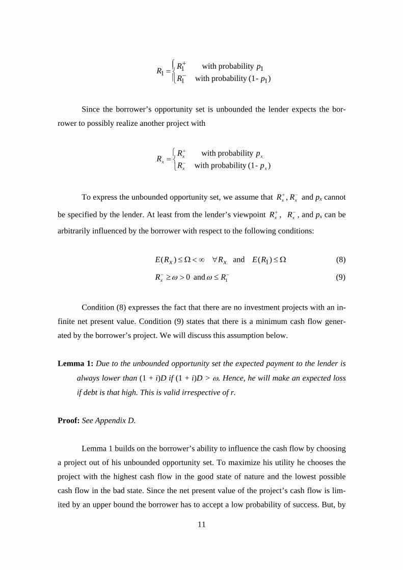
Since the borrower’s opportunity set is unbounded the lender expects the bor-

rower to possibly realize another project with

=−

+

)-(1y probabilitwith y probabilitwith

xx

xxx pR

pRR

To express the unbounded opportunity set, we assume that −+xx RR , and px cannot

be specified by the lender. At least from the lender’s viewpoint +xR , −

xR , and px can be

arbitrarily influenced by the borrower with respect to the following conditions:

)( xx RRE ∀∞<Ω≤ and Ω≤)( 1RE (8)

−− ≤>≥ 1 and 0 RRx ωω (9)

Condition (8) expresses the fact that there are no investment projects with an in-

finite net present value. Condition (9) states that there is a minimum cash flow gener-

ated by the borrower’s project. We will discuss this assumption below.

Lemma 1: Due to the unbounded opportunity set the expected payment to the lender is

always lower than (1 + i)D if (1 + i)D > ω. Hence, he will make an expected loss

if debt is that high. This is valid irrespective of r.

Proof: See Appendix D.

Lemma 1 builds on the borrower’s ability to influence the cash flow by choosing

a project out of his unbounded opportunity set. To maximize his utility he chooses the

project with the highest cash flow in the good state of nature and the lowest possible

cash flow in the bad state. Since the net present value of the project’s cash flow is lim-

ited by an upper bound the borrower has to accept a low probability of success. But, by

12

minimizing the payment to the lender in the bad state he maximizes the dilution of the

lender’s position and hence increases his own wealth if the total expected cash flow is

constant or decreases not to much. With an unbounded opportunity set the borrower has

the possibility to follow this policy. To maximize his utility he will choose a project

with an expected cash flow as high as Ω and with very high risk, in the sense of default

probability, such that the lender’s position is worth not much more than ω.

Lemma 1 leads directly to the following proposition:

Proposition 4: With an unbounded opportunity set the maximum debt is i

D+

=1maxω .

Hence, the lender never takes a risk even though he is risk-neutral.

Proof: The proof follows directly from lemma 1.

A rational lender only provides capital for an investment project if the expected

change in his wealth position is not negative. But, due to the unbounded borrower’s

opportunity set, the lender cannot avoid an expected loss if he takes any risk, no matter

what lending rate he demands.

The only way to induce a lender to provide capital is thus to make his debt posi-

tion risk-free. This can be done only by limiting the debt to the present value of the

lower bound ω of the cash flow. Where does this value come from? In principle the

lower bound of the cash flow is always zero if, e.g., the borrower can carry all the

money into a casino. Hence, a value of 0>ω can be interpreted as the result of some

collateral requirements. Besides the already mentioned sureties the main form of collat-

eral is the limitation of the borrower’s property rights over his assets. That is, the bor-

rower gives up the right to sell an asset serving as security. Furthermore, in case of de-

fault the ownership of this asset is shifted automatically to the lender.7 By this construc-

tion the lender is assured to get at least the liquidation value of the asset no matter

7 In case of a trade credit the lender sells an asset usually with a reservation of proprietary rights to the

borrower. That means that the borrower does not get the property right over the asset until he has fully

paid for it.

13

which action the borrower takes. Thus, that kind of collateral serves as a mechanism to

limit the borrower’s space of action.

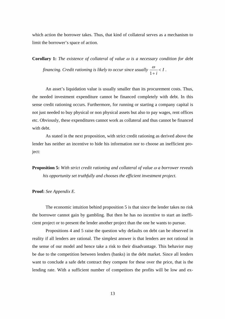
Corollary 1: The existence of collateral of value ω is a necessary condition for debt

financing. Credit rationing is likely to occur since usually Ii<

+1ω .

An asset’s liquidation value is usually smaller than its procurement costs. Thus,

the needed investment expenditure cannot be financed completely with debt. In this

sense credit rationing occurs. Furthermore, for running or starting a company capital is

not just needed to buy physical or non physical assets but also to pay wages, rent offices

etc. Obviously, these expenditures cannot work as collateral and thus cannot be financed

with debt.

As stated in the next proposition, with strict credit rationing as derived above the

lender has neither an incentive to hide his information nor to choose an inefficient pro-

ject:

Proposition 5: With strict credit rationing and collateral of value ω a borrower reveals

his opportunity set truthfully and chooses the efficient investment project.

Proof: See Appendix E.

The economic intuition behind proposition 5 is that since the lender takes no risk

the borrower cannot gain by gambling. But then he has no incentive to start an ineffi-

cient project or to present the lender another project than the one he wants to pursue.

Propositions 4 and 5 raise the question why defaults on debt can be observed in

reality if all lenders are rational. The simplest answer is that lenders are not rational in

the sense of our model and hence take a risk to their disadvantage. This behavior may

be due to the competition between lenders (banks) in the debt market. Since all lenders

want to conclude a safe debt contract they compete for these over the price, that is the

lending rate. With a sufficient number of competitors the profits will be low and ex-

14

panding to the market of risky debt might appear to be a strategy to raise profits. How-

ever, as we have shown, this strategy leads to an expected loss.

But even collateral may not be safe. In case of sureties the default risk is simply

shifted from the project to the borrower (or who ever is the guarantor). Thus, risk cannot

be excluded. If collateral consists of securities in the form of rights over assets there

may also be a risk for the lender. That is because an asset’s liquidation value is risky.

However, this risk can be reduced by a “conservative” estimation of the asset’s liquida-

tion value. Such a conservative estimation can be found in the company’s balance sheet.

This explains the predominance of balance sheet ratios in the credit allowance process.

4 Lender-information From casual observations we know that not every debt contract is secured by

collateral. How can this be explained in the light of our model? So far we have inter-

preted ω as the minimum payment resulting from the investment project which can be

signaled truthfully to the lender. Thus, the natural interpretation of ω is the price of

assets which can be realized on a secondary market. Using assets as securities was nec-

essary since the borrower has a superior information about his type or the set of possible

actions while the lender has no information about the project at all. However, in our

view the assumption of this single-sided information asymmetry is not always appropri-

ate.

Especially institutional investors such as banks or venture capital companies

may have relevant information for the assessment of an investment project due to their

experience. If such an investor infers from his information a minimum cash flow of the

project collateral loses its importance. The assessment of the investor is thus a further

signal about the project quality which the borrower could take into account. He should

do so if the signal is undistorted. That is the lender has no incentive to under- or over-

state his private information in order to raise the price of debt.8 However, if risk avoid-

ance is the lender’s main objective, the signal is undistorted and can directly be used by

the borrower to update his expectations about the profitability of his investment project.

To see this, simply imagine the payoff of a bank assessing a presented investment pro-

8 See Houben (2001) for a discussion of this problem.

15

ject with a specified capital need. If the bank comes to the conclusion that the project

will have a minimum cash flow lower than the needed capital it will face an expected

loss if it grants a higher unsecured debt. On the other hand, with debt lower than the

minimum cash flow or even more by rejecting the borrowers request for debt, the bank

loses a (nearly) risk-less investment opportunity. Thus, the borrower can conclude from

the offered contract the minimum cash flow the bank expects. Hence, he can update his

expectation about the distribution of the future cash flow.

However, the bank’s expectation about the minimum future cash flow can of

course be wrong. Thus, if the bank overestimates the future minimum cash flow a debt

default might appear.

5 Conclusion

In our paper we have shown that in the “classic” debt financing models credit ra-

tioning can but need not occur, depending on the specifications of the assumptions. The

function of credit rationing is limited to a reaction to the endogenous risk for the lender

resulting from the informational asymmetry. However, these models cannot explain

convincingly the use of collateral in debt contracts. That is because credit rationing

alone is in principle a sufficient answer to the problems resulting from information

asymmetry. Furthermore, the lender is not prevented from taking some part of the ex-

ogenous risk.

These results are no longer valid if an unbounded opportunity set is assumed.

Then, only strict credit rationing in combination with the use of collateral is the ade-

quate answer to the generalized moral hazard problem. Credit is rationed to the mini-

mum value of the debt contract safeguarded by the use of collateral. If the lender grants

a higher credit he must expect a loss since there is always a project which improves the

borrower’s position by diluting the lender’s one. The avoidance of risk is the only ra-

tional strategy for lenders in case of pure debt.

Debt defaults are mostly a consequence of the intentionally risk taking by lend-

ers and could thus be avoided by the rational strategy described above.

16

6 Appendix

6.1 Appendix A

If ( ) DiR ⋅+>− 11 the minimum cash flow exceeds the payback obligation. Obvi-

ously the debt is not risky. Furthermore, the type-1-borrower does not seek a credit

since )()1()1()( 1 DIiDiRE −⋅+<⋅+− is valid by assumption.

If ( ) −− <⋅+< 21 1 RDiR and the type-1-borrower does not seek finance the mini-

mum cash flow exceeds again the payback obligation. Obviously the debt is not risky.

Suppose now that ( ) DiR ⋅+<− 12 and both borrowers seek financing. To see that

credit rationing then can occur we first have to calculate Dmax, i.e. the maximum debt

amount a type-2-borrower wants to raise. From (5) and (7) we obtain for the maximum

and minimum lending rate

rDpqpq

RpqRpqpqpq

i+=

⋅⋅−+⋅⋅−⋅−+⋅−⋅

−⋅−+⋅

+ −−

1))1((

)1()1()1()1(

1

21

2211

21

(A1)

rp

iDp

IiRp+≥

++

⋅⋅+−⋅ +

11)1(

22

22 (A2)

We can now calculate Dmax by inserting the left hand side of (A2) for 1+r in

(A1). After rearranging, we obtain

)())1((

)1()()]()1())1(([

12

21

12

211212max ppq

Ipqpqippq

REqRpRpqpD−⋅

⋅⋅−+⋅−

+⋅−⋅⋅−+⋅−+⋅⋅⋅

=−+

(A3)

Credit rationing occurs if

Dmax < I

IiRRqpREqREq

IiREqRpRpq

⋅+<−⋅−⋅−+⋅⇔

⋅+<⋅−+⋅−+⋅⋅⇔++

−+

)1()()()1()(

)1()()1())1((

21121

21121 (A4)

17

Since )( 211++ −⋅ RRqp is positive by assumption, a negative average net present

value IiREqREq ⋅+−⋅−+⋅ )1()()1()( 21 is sufficient for credit rationing to occur.

Q.E.D.

6.2 Appendix B

For ID = the borrowers’ participation constraints ((6) and (7)) are both fulfilled

as long as +≤+ 2)1( RDr . With this upper bound for the borrowers’ obligation the

lender’s participation constraint (5) is also fulfilled, given the distribution of borrowers

asking for credit, if IiRRqpREqRqE )1()()()1()( 21121 +≥−−−+ ++ . Since )( 21++ − RR is

positive by assumption, the average IiREqRqE )1()()1()( 21 +−−+ has to be positive

and must not be less than )( 211++ −⋅ RRqp . This leads to the requirement of

)( 21++ − RR being „small“, which is the case if the variances of 1R and 2R do not differ

much.

Q.E.D.

6.3 Appendix C

For E(R1) < (1 + i)I the lender wants to prevent the borrower from choosing pro-

ject 1 since then he could not break even ex ante. The borrower’s project choice de-

pends on the payback obligation (1 + r)D. He chooses project 2 if

1. −<⋅+ 1)1( RDr since then the debt is risk free and the borrower cannot gain by gam-

bling. The lending rate is equal to risk-free-rate, r = i, and the maximum debt for

which this condition is fulfilled is

iRDa

+=

−

11

max . (A5)

2. −− <⋅+< 21 )1( RDrR and if

DrpRpRE

DrpRpDrRE

⋅+⋅−+⋅>⇔

⋅+⋅−⋅>⋅+−+

+

)1()1()(

)1()1()(

1112

1112

18

Then the debt is risk free again and r = i. The maximum debt for which this condi-

tion is fulfilled is

)1()1()(

1

112max ip

RpREDb

+⋅−⋅−

=+

(A6)

3. +− <⋅+≤ 22 )1( RDrR and if9

cDrpp

RpRp

DrpRpDrpRp

max12

1122

111222

)1(

)1()1()1(

⋅+>−

⋅−⋅⇔

⋅+⋅−⋅>⋅+⋅−−⋅++

++

(A7)

where r is derived from the lender’s participation constraint

−

−

⋅−

−⋅+

=⋅+⇔

⋅+=⋅−+⋅+⋅

22

2

2

222

11)1(

)1()1()1(

Rp

pDp

iDr

DiRpDrp. (A8)

Setting cDrDr max)1()1( ⋅+=⋅+ in (A8) and equalizing (A7) and (A8) leads to

iRp

ippRpRppDc

+⋅−

++⋅−⋅−⋅⋅

=−++

1)1(

)1()()( 22

12

11222max (A9)

Thus, the borrower chooses project 2 if the debt does not exceed the maximum

of the three value cba DDD maxmaxmax and , , and project 1 otherwise. Since the choice of pro-

ject 1 should be prevented credit rationing must occur if

IDDD cba <,,max maxmaxmax

9 Since −+ > 21 RR for p2 < p1 the borrower chooses project 1. Condition (A7) is thus only valid for p2 > p1.

19

If both projects are efficient the lender does not care about the project choice. He

can always break even ex ante by adjusting the lending rate accordingly to the antici-

pated project choice. Since he can anticipate the project choice correctly there is obvi-

ously no room for credit rationing.

Q.E.D.

6.4 Appendix D

We first have to show that there exist combinations of −+xx RR , and px such that

the borrower prefers project x to project 1. He does so if10

DrRRpDrpREp

DrRpDrRp

xx

xx

⋅+−⋅−−⋅+⋅−

>⇔

⋅+−⋅>⋅+−⋅

+

−

++

)1()1()1()(

))1(())1((

1111

11

(A10)

By assumption Project x has to fulfill the following condition

−+

−

−−Ω

≤⇔

Ω≤

xx

xx

x

RRR

p

RE )( (A11)

Hence, there is an infinite number of probabilities px and thus of projects of type

x which the borrower prefers if

][])1()1()([])1([][

)1()1()1()(

1111

1111

−+−+−

+

−

−+

−

−⋅⋅−−⋅+⋅−>⋅+−⋅−Ω⇔

⋅+−⋅−−⋅+⋅−

>−−Ω

xxxx

xxx

x

RRRpDrpREDrRR

DrRRpDrpRE

RRR

(A12)

Note that both sides of the inequality monotonically increase in +xR but that for a suffi-

ciently small −xR the left hand side of the inequality increases faster in +

xR . That is be-

10 We implicitly assume .)1( and )1( 1 DrRRDrR xx ⋅+>>⋅+> +−+ . This is for simplicity purpose only.

20

cause then −− ⋅−−⋅+⋅−>−Ω 1111 )1()1()( RpDrpRERx . Thus, there is an infinite num-

ber of probabilities satisfying (A10) and (A11). The existence of the arbitrary many

projects with a higher expected residual for the borrower is guaranteed11

Next we have to analyze how the borrower will choose +xR . His maximization

problem is

[ ]

);[)(..

max!)1()(

max!))1((

,,

,,

+−

−−

+

∈Ω≤

→−−⋅+−⇔

→⋅+−⋅

−+

−+

xxx

pRRxxxx

pRRxx

RRandREts

RRDrpRE

DrRp

xxx

xxx

ω

(A13)

It follows immediately that the solution is

p R xx ,0, →→− ω and ∞→+xR .

It is now easy to see that the lender faces an expected loss if (1+i) D > ω. We have

−

−

−

−⋅+−⋅+

<⇔

⋅+<⋅−+⋅+⋅

x

xx

xxx

RDrRDip

DiRpDrp

)1()1(

)1()1()1(

which is

DiDrDi

⋅+<⇔−⋅+−⋅+

< )1()1()1(0 ω

ωω

given the above solution of the borrower’s maximization problem.

Q.E.D

11 Note that for +>⋅+ 1)1( RDr (A10) simplifies to px > 0 such that the proof of existence of px satisfying

(A10) and (A11) is already done since 0>−Ω −xR .

21

6.5 Appendix E

Without a lender taking risk, which is assured by credit rationing and collateral,

the borrower has no incentive to choose an inefficient project. Formally he will only

seek finance for a project if

IiREDIiDiRE

⋅+>−⋅+>⋅+−

)1()()()1()1()(

(A15)

which is exactly the efficiency constraint. Furthermore, since the borrower maximizes

his wealth he will choose the project with the maximum net present value. But, if the

borrower chooses the efficient project anyway, there is no incentive for him to present

another project the lender.

Q.E.D.

22

References

BESTER, H. (1985): Screening vs. Rationing in Credit Markets with Imperfect Informa-

tion, American Economic Review, 75, 850-859.

BESTER, H. AND M. HELLWIG (1987): Moral Hazard and Equilibrium Credit Rationing.

In Agency Theory, Information, and Incentives, edited by Bamberg, G. and K.

Spremann, 135-166.

HART, O. AND J. MOORE (1994): A Theory of Debt Based on the Inalienability of Hu-

man Capital, Quarterly Journal of Economics, 109, 841-879.

HART, O. AND J. MOORE (1998): Default and Renegotiation: A Dynamic Model of Debt,

Quarterly Journal of Economics, 113, 1-41.

HOUBEN, E. (2001): Venture Capital, Double-sided Moral Hazard, and Double-sided

Adverse Selection, working paper, University of Kiel.

JENSEN, M. C. AND W. H. MECKLING (1976): Theory of the Firm: Managerial Behavior,

Agency Costs, and Ownership Structure, Journal of Financial Economics, 3, 305-

360.

NEUS, W. (1998): Kreditsicherheiten und Modelle der Kreditfinanzierung. In Unter-

nehmensführung und Kapitalmarkt, edited by Franke, G. and H. Laux, 211-251.

RAVID, S. A. AND M. SPIEGEL (1997): Optimal Financial Contracts for a Start-Up with

Unlimited Operating Discretion, Journal of Financial and Quantitative Analysis,

32, 269-286.

STIGLITZ, J. E. AND A. WEISS (1981): Credit Rationing in Markets with Imperfect In-

formation, American Economic Review, 71, 393-410.